series mc lauren for electronics switch calculations such as IC components and microcontroler AMNIMARJESLOW GOVERNMENT 91220017 XI XA PIN PING HUNG CHOP 02096010014 LJBUSAF series as like as connection ; series not balancing $2

in the time-controlled electronics science or so-called timing process known to many electronic components that serve for timing control process such as: transistor, Integrated circuit, microprocessor and micro controller software program outside the flow chart hardware process of component components mentioned above should be reviewed system work and work quality of components of process components in integrated electronics circuits such as transistors, both silicon, germanium, optical fiber transistors (opto coupler) as well as all solid state equipment and power electronics such as thyristior all components of above electronic components need to be calculated and reviewed performance in the current technological advances especially in the flowchart process of the control system of the time and responsiveness of the component so that it can be made to search for certain materials for the above mentioned components of electronic components for the benefit of external program space and re set of earth programs. in the future we will enter nano, pico and soft processor and control .

                                     

                                                             Taylor series

 In mathematics, a Taylor series is a representation of a function as an infinite sum of terms that are calculated from the values of the function's derivatives at a single point.

The concept of a Taylor series was formulated by the Scottish mathematician James Gregory and formally introduced by the English mathematician Brook Taylor in 1715. If the Taylor series is centered at zero, then that series is also called aMaclaurin series, named after the Scottish mathematician Colin Maclaurin, who made extensive use of this special case of Taylor series in the 18th century.

A function can be approximated by using a finite number of terms of its Taylor series. Taylor's theorem gives quantitative estimates on the error introduced by the use of such an approximation. The polynomial formed by taking some initial terms of the Taylor series is called a Taylor polynomial. The Taylor series of a function is the limit of that function's Taylor polynomials as the degree increases, provided that the limit exists. A function may not be equal to its Taylor series, even if its Taylor seriesconverges at every point. A function that is equal to its Taylor series in an open interval (or a disc in the complex plane) is known as an analytic function in that interval. 

                               

 

                                

The exponential function e^x (in blue), and the sum of the first n + 1terms of its Taylor series at 0 (in red).  

The Taylor series of a real or complex-valued function f (x) that is infinitely differentiable at a real or complex number a is the power series

Definition

${\displaystyle f(a)+{\frac {f'(a)}{1!}}(x-a)+{\frac {f''(a)}{2!}}(x-a)^{2}+{\frac {f'''(a)}{3!}}(x-a)^{3}+\cdots .}$

which can be written in the more compact sigma notation as

${\displaystyle \sum _{n=0}^{\infty }{\frac {f^{(n)}(a)}{n!}}\,(x-a)^{n}}$

where n! denotes the factorial of n and f⁽ⁿ⁾(a) denotes the nth derivative of f evaluated at the point a. The derivative of order zero off is defined to be f itself and (x − a)⁰ and 0! are both defined to be 1. When a = 0, the series is also called a Maclaurin series.

The Taylor series for any polynomial is the polynomial itself.

Examples

The Maclaurin series for 1/1 − x is the geometric series

${\displaystyle 1+x+x^{2}+x^{3}+\cdots \!}$

so the Taylor series for 1/x at a = 1 is

${\displaystyle 1-(x-1)+(x-1)^{2}-(x-1)^{3}+\cdots .\!}$

By integrating the above Maclaurin series, we find the Maclaurin series for log(1 − x), where log denotes the natural logarithm:

${\displaystyle -x-{\tfrac {1}{2}}x^{2}-{\tfrac {1}{3}}x^{3}-{\tfrac {1}{4}}x^{4}-\cdots \!}$

and the corresponding Taylor series for log x at a = 1 is

${\displaystyle (x-1)-{\tfrac {1}{2}}(x-1)^{2}+{\tfrac {1}{3}}(x-1)^{3}-{\tfrac {1}{4}}(x-1)^{4}+\cdots ,\!}$

and more generally, the corresponding Taylor series for log x at some a = x₀ is:

${\displaystyle \log(x_{0})+{\frac {1}{x_{0}}}(x-x_{0})-{\frac {1}{x_{0}^{2}}}{\frac {\left(x-x_{0}\right)^{2}}{2}}+\cdots .}$

The Taylor series for the exponential function e^x at a = 0 is

${\displaystyle {\frac {x^{0}}{0!}}+{\frac {x^{1}}{1!}}+{\frac {x^{2}}{2!}}+{\frac {x^{3}}{3!}}+{\frac {x^{4}}{4!}}+{\frac {x^{5}}{5!}}+\cdots =1+x+{\frac {x^{2}}{2}}+{\frac {x^{3}}{6}}+{\frac {x^{4}}{24}}+{\frac {x^{5}}{120}}+\cdots \!=\sum _{n=0}^{\infty }{\frac {x^{n}}{n!}}.}$

The above expansion holds because the derivative of e^x with respect to x is also e^x and e⁰ equals 1. This leaves the terms (x − 0)ⁿ in the numerator and n! in the denominator for each term in the infinite 

The Greek philosopher Zeno considered the problem of summing an infinite series to achieve a finite result, but rejected it as an impossibility^{[citation needed]}: the result was Zeno's paradox. Later, Aristotle proposed a philosophical resolution of the paradox, but the mathematical content was apparently unresolved until taken up by Archimedes, as it had been prior to Aristotle by the Presocratic Atomist Democritus. It was through Archimedes's method of exhaustion that an infinite number of progressive subdivisions could be performed to achieve a finite result.^[1] Liu Hui independently employed a similar method a few centuries later.^[2]

In the 14th century, the earliest examples of the use of Taylor series and closely related methods were given by Madhava of Sangamagrama.^[3][4] Though no record of his work survives, writings of later Indian mathematicians suggest that he found a number of special cases of the Taylor series, including those for the trigonometric functions of sine,cosine, tangent, and arctangent. The Kerala School of Astronomy and Mathematics further expanded his works with various series expansions and rational approximations until the 16th century.

In the 17th century, James Gregory also worked in this area and published several Maclaurin series. It was not until 1715 however that a general method for constructing these series for all functions for which they exist was finally provided by Brook Taylor,^[5] after whom the series are now named.

The Maclaurin series was named after Colin Maclaurin, a professor in Edinburgh, who published the special case of the Taylor result in the 18th century.

Analytic functions

The function e^(−1/x2) is not analytic at x = 0: the Taylor series is identically 0, although the function is not.

If f (x) is given by a convergent power series in an open disc (or interval in the real line) centered at b in the complex plane, it is said to be analytic in this disc. Thus for x in this disc, f is given by a convergent power series

${\displaystyle f(x)=\sum _{n=0}^{\infty }a_{n}(x-b)^{n}.}$

Differentiating by x the above formula n times, then setting x = b gives:

${\displaystyle {\frac {f^{(n)}(b)}{n!}}=a_{n}}$

and so the power series expansion agrees with the Taylor series. Thus a function is analytic in an open disc centered at b if and only if its Taylor series converges to the value of the function at each point of the disc.

If f (x) is equal to its Taylor series for all x in the complex plane, it is called entire. The polynomials, exponential function e^x, and the trigonometric functions sine and cosine, are examples of entire functions. Examples of functions that are not entire include the square root, the logarithm, the trigonometric function tangent, and its inverse, arctan. For these functions the Taylor series do not converge if x is far from b. That is, the Taylor series diverges at x if the distance between x and b is larger than the radius of convergence. The Taylor series can be used to calculate the value of an entire function at every point, if the value of the function, and of all of its derivatives, are known at a single point.

Uses of the Taylor series for analytic functions include:

1. The partial sums (the Taylor polynomials) of the series can be used as approximations of the function. These approximations are good if sufficiently many terms are included.
2. Differentiation and integration of power series can be performed term by term and is hence particularly easy.
3. An analytic function is uniquely extended to a holomorphic function on an open disk in the complex plane. This makes the machinery of complex analysis available.
4. The (truncated) series can be used to compute function values numerically, (often by recasting the polynomial into the Chebyshev form and evaluating it with the Clenshaw algorithm).
5. Algebraic operations can be done readily on the power series representation; for instance, Euler's formula follows from Taylor series expansions for trigonometric and exponential functions. This result is of fundamental importance in such fields as harmonic analysis.
6. Approximations using the first few terms of a Taylor series can make otherwise unsolvable problems possible for a restricted domain; this approach is often used in physics.

Approximation error and convergence

The sine function (blue) is closely approximated by its Taylor polynomial of degree 7 (pink) for a full period centered at the origin.

The Taylor polynomials for log(1 + x) only provide accurate approximations in the range −1 < x ≤ 1. Note that, for x > 1, the Taylor polynomials of higher degree are worse approximations.

The Taylor approximations for log(1 + x) (black). For x > 1, the approximations diverge.

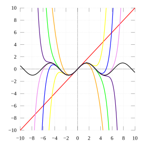
Pictured on the right is an accurate approximation of sin x around the point x = 0. The pink curve is a polynomial of degree seven:

${\displaystyle \sin \left(x\right)\approx x-{\frac {x^{3}}{3!}}+{\frac {x^{5}}{5!}}-{\frac {x^{7}}{7!}}.\!}$

The error in this approximation is no more than |x|⁹/9!. In particular, for −1 < x < 1, the error is less than 0.000003.

In contrast, also shown is a picture of the natural logarithm function log(1 + x) and some of its Taylor polynomials arounda = 0. These approximations converge to the function only in the region −1 < x ≤ 1; outside of this region the higher-degree Taylor polynomials are worse approximations for the function. This is similar to Runge's phenomenon.

The error incurred in approximating a function by its nth-degree Taylor polynomial is called the remainder or residual and is denoted by the function R_n(x). Taylor's theorem can be used to obtain a bound on the size of the remainder.

In general, Taylor series need not be convergent at all. And in fact the set of functions with a convergent Taylor series is ameager set in the Fréchet space of smooth functions. And even if the Taylor series of a function f does converge, its limit need not in general be equal to the value of the function f (x). For example, the function

${\displaystyle f(x)={\begin{cases}e^{-{\frac {1}{x^{2}}}}&{\text{if }}x\neq 0\\0&{\text{if }}x=0\end{cases}}}$

is infinitely differentiable at x = 0, and has all derivatives zero there. Consequently, the Taylor series of f (x) about x = 0 is identically zero. However, f (x) is not the zero function, so does not equal its Taylor series around the origin. Thus, f (x) is an example of a non-analytic smooth function.

In real analysis, this example shows that there are infinitely differentiable functions f (x) whose Taylor series are not equal tof (x) even if they converge. By contrast, the holomorphic functions studied in complex analysis always possess a convergent Taylor series, and even the Taylor series of meromorphic functions, which might have singularities, never converge to a value different from the function itself. The complex function e^−1/z2, however, does not approach 0 when z approaches 0 along the imaginary axis, so it is not continuous in the complex plane and its Taylor series is undefined at 0.

More generally, every sequence of real or complex numbers can appear as coefficients in the Taylor series of an infinitely differentiable function defined on the real line, a consequence of Borel's lemma. As a result, the radius of convergence of a Taylor series can be zero. There are even infinitely differentiable functions defined on the real line whose Taylor series have a radius of convergence 0 everywhere.

Some functions cannot be written as Taylor series because they have a singularity; in these cases, one can often still achieve a series expansion if one allows also negative powers of the variable x; see Laurent series. For example, f (x) = e^−1/x2 can be written as a Laurent series.

There is, however, a generalization^[7][8] of the Taylor series that does converge to the value of the function itself for anybounded continuous function on (0,∞), using the calculus of finite differences. Specifically, one has the following theorem, due to Einar Hille, that for any t > 0,

Generalization

${\displaystyle \lim _{h\to 0^{+}}\sum _{n=0}^{\infty }{\frac {t^{n}}{n!}}{\frac {\Delta _{h}^{n}f(a)}{h^{n}}}=f(a+t).}$

Here Δⁿ
_h is the nth finite difference operator with step size h. The series is precisely the Taylor series, except that divided differences appear in place of differentiation: the series is formally similar to the Newton series. When the function f is analytic at a, the terms in the series converge to the terms of the Taylor series, and in this sense generalizes the usual Taylor series.

In general, for any infinite sequence a_i, the following power series identity holds:

${\displaystyle \sum _{n=0}^{\infty }{\frac {u^{n}}{n!}}\Delta ^{n}a_{i}=e^{-u}\sum _{j=0}^{\infty }{\frac {u^{j}}{j!}}a_{i+j}.}$

So in particular,

${\displaystyle f(a+t)=\lim _{h\to 0^{+}}e^{-{\frac {t}{h}}}\sum _{j=0}^{\infty }f(a+jh){\frac {\left({\frac {t}{h}}\right)^{j}}{j!}}.}$

The series on the right is the expectation value of f (a + X), where X is a Poisson-distributed random variable that takes the value jh with probability e^−t/h·(t/h)^j/j!. Hence,

${\displaystyle f(a+t)=\lim _{h\to 0^{+}}\int _{-\infty }^{\infty }f(a+x)dP_{{\frac {t}{h}},h}(x).}$

The law of large numbers implies that the identity holds.

List of Maclaurin series of some common functions

The real part of the cosine function in thecomplex plane

An 8th-degree approximation of the cosine function in thecomplex plane

The two above curves put together

Several important Maclaurin series expansions follow.^[10] All these expansions are valid for complex arguments x.

The exponential function  (with base e) has Maclaurin series

Exponential function

${\displaystyle e^{x}=\sum _{n=0}^{\infty }{\frac {x^{n}}{n!}}=1+x+{\frac {x^{2}}{2!}}+{\frac {x^{3}}{3!}}+\cdots }$.

It converges for all x.

The natural logarithm (with base e) has Maclaurin series

Natural logarithm

${\displaystyle {\begin{aligned}\log(1-x)&=-\sum _{n=1}^{\infty }{\frac {x^{n}}{n}}=-x-{\frac {x^{2}}{2}}-{\frac {x^{3}}{3}}-\cdots ,\\\log(1+x)&=\sum _{n=1}^{\infty }(-1)^{n+1}{\frac {x^{n}}{n}}=x-{\frac {x^{2}}{2}}+{\frac {x^{3}}{3}}-\cdots .\end{aligned}}}$

They converge for ${\displaystyle |x|<1}$.

The geometric series and its derivatives have Maclaurin series

Geometric series

${\displaystyle {\begin{aligned}{\frac {1}{1-x}}&=\sum _{n=0}^{\infty }x^{n}\\{\frac {1}{(1-x)^{2}}}&=\sum _{n=1}^{\infty }nx^{n-1}\\{\frac {1}{(1-x)^{3}}}&=\sum _{n=2}^{\infty }{\frac {(n-1)n}{2}}x^{n-2}.\end{aligned}}}$

All are convergent for ${\displaystyle |x|<1}$. These are special cases of the binomial series given in the next section.

The binomial series is the power series

Binomial series

${\displaystyle (1+x)^{\alpha }=\sum _{n=0}^{\infty }{\binom {\alpha }{n}}x^{n}}$

whose coefficients are the generalized binomial coefficients

${\displaystyle {\binom {\alpha }{n}}=\prod _{k=1}^{n}{\frac {\alpha -k+1}{k}}={\frac {\alpha (\alpha -1)\cdots (\alpha -n+1)}{n!}}.}$

(If n = 0, this product is an empty product and has value 1.) It converges for ${\displaystyle |x|<1}$ for any real or complex number α.

When α = −1, this is essentially the infinite geometric series mentioned in the previous section. The special cases α = 1/2 and α = −1/2 give the square root function and its inverse:

${\displaystyle {\begin{aligned}(1+x)^{\frac {1}{2}}&=1+{\tfrac {1}{2}}x-{\tfrac {1}{8}}x^{2}+{\tfrac {1}{16}}x^{3}-{\tfrac {5}{128}}x^{4}+{\tfrac {7}{256}}x^{5}-\ldots ,\\(1+x)^{-{\frac {1}{2}}}&=1-{\tfrac {1}{2}}x+{\tfrac {3}{8}}x^{2}-{\tfrac {5}{16}}x^{3}+{\tfrac {35}{128}}x^{4}-{\tfrac {63}{256}}x^{5}+\ldots .\end{aligned}}}$

The usual trigonometric functions and their inverses have the following Maclaurin series:

Trigonometric functions

${\displaystyle {\begin{aligned}\sin x&=\sum _{n=0}^{\infty }{\frac {(-1)^{n}}{(2n+1)!}}x^{2n+1}&&=x-{\frac {x^{3}}{6}}+{\frac {x^{5}}{120}}-\cdots &&{\text{for all }}x\\[6pt]\cos x&=\sum _{n=0}^{\infty }{\frac {(-1)^{n}}{(2n)!}}x^{2n}&&=1-{\frac {x^{2}}{2}}+{\frac {x^{4}}{24}}-\cdots &&{\text{for all }}x\\[6pt]\tan x&=\sum _{n=1}^{\infty }{\frac {B_{2n}(-4)^{n}\left(1-4^{n}\right)}{(2n)!}}x^{2n-1}&&=x+{\frac {x^{3}}{3}}+{\frac {2x^{5}}{15}}+\cdots &&{\text{for }}|x|<{\frac {\pi }{2}}\\[6pt]\sec x&=\sum _{n=0}^{\infty }{\frac {(-1)^{n}E_{2n}}{(2n)!}}x^{2n}&&=1+{\frac {x^{2}}{2}}+{\frac {5x^{4}}{24}}+\cdots &&{\text{for }}|x|<{\frac {\pi }{2}}\\[6pt]\arcsin x&=\sum _{n=0}^{\infty }{\frac {(2n)!}{4^{n}(n!)^{2}(2n+1)}}x^{2n+1}&&=x+{\frac {x^{3}}{6}}+{\frac {3x^{5}}{40}}+\cdots &&{\text{for }}|x|\leq 1\\[6pt]\arccos x&={\frac {\pi }{2}}-\arcsin x\\&={\frac {\pi }{2}}-\sum _{n=0}^{\infty }{\frac {(2n)!}{4^{n}(n!)^{2}(2n+1)}}x^{2n+1}&&={\frac {\pi }{2}}-x-{\frac {x^{3}}{6}}-{\frac {3x^{5}}{40}}+\cdots &&{\text{for }}|x|\leq 1\\[6pt]\arctan x&=\sum _{n=0}^{\infty }{\frac {(-1)^{n}}{2n+1}}x^{2n+1}&&=x-{\frac {x^{3}}{3}}+{\frac {x^{5}}{5}}-\cdots &&{\text{for }}|x|\leq 1,\ x\neq \pm i\end{aligned}}}$

All angles are expressed in radians. The numbers B_k appearing in the expansions of tan x are the Bernoulli numbers. The E_k in the expansion of sec x are Euler numbers.

The hyperbolic functions have Maclaurin series closely related to the series for the corresponding trigonometric functions:

Hyperbolic functions

${\displaystyle {\begin{aligned}\sinh x&=\sum _{n=0}^{\infty }{\frac {x^{2n+1}}{(2n+1)!}}&&=x+{\frac {x^{3}}{3!}}+{\frac {x^{5}}{5!}}+\cdots &&{\text{for all }}x\\[6pt]\cosh x&=\sum _{n=0}^{\infty }{\frac {x^{2n}}{(2n)!}}&&=1+{\frac {x^{2}}{2!}}+{\frac {x^{4}}{4!}}+\cdots &&{\text{for all }}x\\[6pt]\tanh x&=\sum _{n=1}^{\infty }{\frac {B_{2n}4^{n}\left(4^{n}-1\right)}{(2n)!}}x^{2n-1}&&=x-{\frac {x^{3}}{3}}+{\frac {2x^{5}}{15}}-{\frac {17x^{7}}{315}}+\cdots &&{\text{for }}|x|<{\frac {\pi }{2}}\\[6pt]\operatorname {arsinh} x&=\sum _{n=0}^{\infty }{\frac {(-1)^{n}(2n)!}{4^{n}(n!)^{2}(2n+1)}}x^{2n+1}&&&&{\text{for }}|x|\leq 1\\[6pt]\operatorname {artanh} x&=\sum _{n=0}^{\infty }{\frac {x^{2n+1}}{2n+1}}&&&&{\text{for }}|x|\leq 1,\ x\neq \pm 1\end{aligned}}}$

The numbers B_k appearing in the series for tanh x are the Bernoulli numbers.

Several methods exist for the calculation of Taylor series of a large number of functions. One can attempt to use the definition of the Taylor series, though this often requires generalizing the form of the coefficients according to a readily apparent pattern. Alternatively, one can use manipulations such as substitution, multiplication or division, addition or subtraction of standard Taylor series to construct the Taylor series of a function, by virtue of Taylor series being power series. In some cases, one can also derive the Taylor series by repeatedly applying integration by parts. Particularly convenient is the use of computer algebra systems to calculate Taylor series.

Calculation of Taylor series

In order to compute the 7th degree Maclaurin polynomial for the function

First example

${\displaystyle f(x)=\log(\cos x),\quad x\in \left(-{\frac {\pi }{2}},{\frac {\pi }{2}}\right)}$ ,

one may first rewrite the function as

${\displaystyle f(x)=\log {\bigl (}1+(\cos x-1){\bigr )}\!}$.

The Taylor series for the natural logarithm is (using the big O notation)

${\displaystyle \log(1+x)=x-{\frac {x^{2}}{2}}+{\frac {x^{3}}{3}}+{O}\left(x^{4}\right)\!}$

and for the cosine function

${\displaystyle \cos x-1=-{\frac {x^{2}}{2}}+{\frac {x^{4}}{24}}-{\frac {x^{6}}{720}}+{O}\left(x^{8}\right)\!}$.

The latter series expansion has a zero constant term, which enables us to substitute the second series into the first one and to easily omit terms of higher order than the 7th degree by using the big O notation:

${\displaystyle {\begin{aligned}f(x)&=\log {\bigl (}1+(\cos x-1){\bigr )}\\&=(\cos x-1)-{\tfrac {1}{2}}(\cos x-1)^{2}+{\tfrac {1}{3}}(\cos x-1)^{3}+{O}\left((\cos x-1)^{4}\right)\\&=\left(-{\frac {x^{2}}{2}}+{\frac {x^{4}}{24}}-{\frac {x^{6}}{720}}+{O}\left(x^{8}\right)\right)-{\frac {1}{2}}\left(-{\frac {x^{2}}{2}}+{\frac {x^{4}}{24}}+{O}\left(x^{6}\right)\right)^{2}+{\frac {1}{3}}\left(-{\frac {x^{2}}{2}}+O\left(x^{4}\right)\right)^{3}+{O}\left(x^{8}\right)\\&=-{\frac {x^{2}}{2}}+{\frac {x^{4}}{24}}-{\frac {x^{6}}{720}}-{\frac {x^{4}}{8}}+{\frac {x^{6}}{48}}-{\frac {x^{6}}{24}}+O\left(x^{8}\right)\\&=-{\frac {x^{2}}{2}}-{\frac {x^{4}}{12}}-{\frac {x^{6}}{45}}+O\left(x^{8}\right).\end{aligned}}\!}$

Since the cosine is an even function, the coefficients for all the odd powers x, x³, x⁵, x⁷, ... have to be zero.

Suppose we want the Taylor series at 0 of the function

Second example

${\displaystyle g(x)={\frac {e^{x}}{\cos x}}.\!}$

We have for the exponential function

${\displaystyle e^{x}=\sum _{n=0}^{\infty }{\frac {x^{n}}{n!}}=1+x+{\frac {x^{2}}{2!}}+{\frac {x^{3}}{3!}}+{\frac {x^{4}}{4!}}+\cdots \!}$

and, as in the first example,

${\displaystyle \cos x=1-{\frac {x^{2}}{2!}}+{\frac {x^{4}}{4!}}-\cdots \!}$

Assume the power series is

${\displaystyle {\frac {e^{x}}{\cos x}}=c_{0}+c_{1}x+c_{2}x^{2}+c_{3}x^{3}+\cdots \!}$

Then multiplication with the denominator and substitution of the series of the cosine yields

${\displaystyle {\begin{aligned}e^{x}&=\left(c_{0}+c_{1}x+c_{2}x^{2}+c_{3}x^{3}+\cdots \right)\cos x\\&=\left(c_{0}+c_{1}x+c_{2}x^{2}+c_{3}x^{3}+c_{4}x^{4}+\cdots \right)\left(1-{\frac {x^{2}}{2!}}+{\frac {x^{4}}{4!}}-\cdots \right)\\&=c_{0}-{\frac {c_{0}}{2}}x^{2}+{\frac {c_{0}}{4!}}x^{4}+c_{1}x-{\frac {c_{1}}{2}}x^{3}+{\frac {c_{1}}{4!}}x^{5}+c_{2}x^{2}-{\frac {c_{2}}{2}}x^{4}+{\frac {c_{2}}{4!}}x^{6}+c_{3}x^{3}-{\frac {c_{3}}{2}}x^{5}+{\frac {c_{3}}{4!}}x^{7}+c_{4}x^{4}+\cdots \end{aligned}}\!}$

Collecting the terms up to fourth order yields

${\displaystyle e^{x}=c_{0}+c_{1}x+\left(c_{2}-{\frac {c_{0}}{2}}\right)x^{2}+\left(c_{3}-{\frac {c_{1}}{2}}\right)x^{3}+\left(c_{4}-{\frac {c_{2}}{2}}+{\frac {c_{0}}{4!}}\right)x^{4}+\cdots \!}$

The values of ${\displaystyle c_{i}}$ can be found by comparison of coefficients with the top expression for ${\displaystyle e^{x}}$, yielding:

${\displaystyle {\frac {e^{x}}{\cos x}}=1+x+x^{2}+{\frac {2x^{3}}{3}}+{\frac {x^{4}}{2}}+\cdots .\!}$

Here we employ a method called "indirect expansion" to expand the given function. This method uses the known Taylor expansion of the exponential function. In order to expand(1 + x)e^x as a Taylor series in x, we use the known Taylor series of function e^x:

Third example

${\displaystyle e^{x}=\sum _{n=0}^{\infty }{\frac {x^{n}}{n!}}=1+x+{\frac {x^{2}}{2!}}+{\frac {x^{3}}{3!}}+{\frac {x^{4}}{4!}}+\cdots .}$

Thus,

${\displaystyle {\begin{aligned}(1+x)e^{x}&=e^{x}+xe^{x}=\sum _{n=0}^{\infty }{\frac {x^{n}}{n!}}+\sum _{n=0}^{\infty }{\frac {x^{n+1}}{n!}}=1+\sum _{n=1}^{\infty }{\frac {x^{n}}{n!}}+\sum _{n=0}^{\infty }{\frac {x^{n+1}}{n!}}\\&=1+\sum _{n=1}^{\infty }{\frac {x^{n}}{n!}}+\sum _{n=1}^{\infty }{\frac {x^{n}}{(n-1)!}}=1+\sum _{n=1}^{\infty }\left({\frac {1}{n!}}+{\frac {1}{(n-1)!}}\right)x^{n}\\&=1+\sum _{n=1}^{\infty }{\frac {n+1}{n!}}x^{n}\\&=\sum _{n=0}^{\infty }{\frac {n+1}{n!}}x^{n}.\end{aligned}}}$

Classically, algebraic functions are defined by an algebraic equation, and transcendental functions (including those discussed above) are defined by some property that holds for them, such as a differential equation. For example, the exponential function is the function which is equal to its own derivative everywhere, and assumes the value 1 at the origin. However, one may equally well define an analytic function by its Taylor series.

Taylor series as definitions

Taylor series are used to define functions and "operators" in diverse areas of mathematics. In particular, this is true in areas where the classical definitions of functions break down. For example, using Taylor series, one may define analytical functions of matrices and operators, such as the matrix exponential or matrix logarithm.

In other areas, such as formal analysis, it is more convenient to work directly with the power series themselves. Thus one may define a solution of a differential equation as a power series which, one hopes to prove, is the Taylor series of the desired solution.

The Taylor series may also be generalized to functions of more than one variable with

Taylor series in several variables

${\displaystyle {\begin{aligned}T(x_{1},\ldots ,x_{d})&=\sum _{n_{1}=0}^{\infty }\cdots \sum _{n_{d}=0}^{\infty }{\frac {(x_{1}-a_{1})^{n_{1}}\cdots (x_{d}-a_{d})^{n_{d}}}{n_{1}!\cdots n_{d}!}}\,\left({\frac {\partial ^{n_{1}+\cdots +n_{d}}f}{\partial x_{1}^{n_{1}}\cdots \partial x_{d}^{n_{d}}}}\right)(a_{1},\ldots ,a_{d})\\&=f(a_{1},\ldots ,a_{d})+\sum _{j=1}^{d}{\frac {\partial f(a_{1},\ldots ,a_{d})}{\partial x_{j}}}(x_{j}-a_{j})+{\frac {1}{2!}}\sum _{j=1}^{d}\sum _{k=1}^{d}{\frac {\partial ^{2}f(a_{1},\ldots ,a_{d})}{\partial x_{j}\partial x_{k}}}(x_{j}-a_{j})(x_{k}-a_{k})+\\&\qquad \qquad +{\frac {1}{3!}}\sum _{j=1}^{d}\sum _{k=1}^{d}\sum _{l=1}^{d}{\frac {\partial ^{3}f(a_{1},\ldots ,a_{d})}{\partial x_{j}\partial x_{k}\partial x_{l}}}(x_{j}-a_{j})(x_{k}-a_{k})(x_{l}-a_{l})+\cdots \end{aligned}}}$

For example, for a function that depends on two variables, x and y, the Taylor series to second order about the point (a, b) is

${\displaystyle f(a,b)+(x-a)f_{x}(a,b)+(y-b)f_{y}(a,b)+{\frac {1}{2!}}{\Big (}(x-a)^{2}f_{xx}(a,b)+2(x-a)(y-b)f_{xy}(a,b)+(y-b)^{2}f_{yy}(a,b){\Big )}}$

where the subscripts denote the respective partial derivatives.

A second-order Taylor series expansion of a scalar-valued function of more than one variable can be written compactly as

${\displaystyle T(\mathbf {x} )=f(\mathbf {a} )+(\mathbf {x} -\mathbf {a} )^{\mathsf {T}}Df(\mathbf {a} )+{\frac {1}{2!}}(\mathbf {x} -\mathbf {a} )^{\mathsf {T}}\left\{D^{2}f(\mathbf {a} )\right\}(\mathbf {x} -\mathbf {a} )+\cdots ,}$

where D f (a) is the gradient of f evaluated at x = a and D² f (a) is the Hessian matrix. Applying the multi-index notation the Taylor series for several variables becomes

${\displaystyle T(\mathbf {x} )=\sum _{|\alpha |\geq 0}{\frac {(\mathbf {x} -\mathbf {a} )^{\alpha }}{\alpha !}}\left({\mathrm {\partial } ^{\alpha }}f\right)(\mathbf {a} ),}$

which is to be understood as a still more abbreviated multi-index version of the first equation of this paragraph, again in full analogy to the single variable case.

Example

Second-order Taylor series approximation (in orange) of a function f (x,y) = e^x log(1 + y)around the origin.

In order to compute a second-order Taylor series expansion around point (a, b) = (0, 0) of the function

${\displaystyle f(x,y)=e^{x}\log(1+y),}$

one first computes all the necessary partial derivatives:

${\displaystyle {\begin{aligned}f_{x}&=e^{x}\log(1+y)\\[6pt]f_{y}&={\frac {e^{x}}{1+y}}\\[6pt]f_{xx}&=e^{x}\log(1+y)\\[6pt]f_{yy}&=-{\frac {e^{x}}{(1+y)^{2}}}\\[6pt]f_{xy}&=f_{yx}={\frac {e^{x}}{1+y}}.\end{aligned}}}$

Evaluating these derivatives at the origin gives the Taylor coefficients

${\displaystyle {\begin{aligned}f_{x}(0,0)&=0\\f_{y}(0,0)&=1\\f_{xx}(0,0)&=0\\f_{yy}(0,0)&=-1\\f_{xy}(0,0)&=f_{yx}(0,0)=1.\end{aligned}}}$

Substituting these values in to the general formula

${\displaystyle T(x,y)=f(a,b)+(x-a)f_{x}(a,b)+(y-b)f_{y}(a,b)+{\frac {1}{2!}}{\Big (}(x-a)^{2}f_{xx}(a,b)+2(x-a)(y-b)f_{xy}(a,b)+(y-b)^{2}f_{yy}(a,b){\Big )}+\cdots }$

produces

${\displaystyle {\begin{aligned}T(x,y)&=0+0(x-0)+1(y-0)+{\frac {1}{2}}{\Big (}0(x-0)^{2}+2(x-0)(y-0)+(-1)(y-0)^{2}{\Big )}+\cdots \\&=y+xy-{\frac {y^{2}}{2}}+\cdots \end{aligned}}}$

Since log(1 + y) is analytic in |y| < 1, we have

${\displaystyle e^{x}\log(1+y)=y+xy-{\frac {y^{2}}{2}}+\cdots ,\qquad |y|<1.}$

Comparison with Fourier series

The trigonometric Fourier series enables one to express a periodic function (or a function defined on a closed interval [a,b]) as an infinite sum of trigonometric functions (sinesand cosines). In this sense, the Fourier series is analogous to Taylor series, since the latter allows one to express a function as an infinite sum of powers. Nevertheless, the two series differ from each other in several relevant issues:

• Obviously the finite truncations of the Taylor series of f (x) about the point x = a are all exactly equal to f at a. In contrast, the Fourier series is computed by integrating over an entire interval, so there is generally no such point where all the finite truncations of the series are exact.
• Indeed, the computation of Taylor series requires the knowledge of the function on an arbitrary small neighbourhood of a point, whereas the computation of the Fourier series requires knowing the function on its whole domain interval. In a certain sense one could say that the Taylor series is "local" and the Fourier series is "global".
• The Taylor series is defined for a function which has infinitely many derivatives at a single point, whereas the Fourier series is defined for any integrable function. In particular, the function could be nowhere differentiable. (For example, f (x) could be a Weierstrass function.)
• The convergence of both series has very different properties. Even if the Taylor series has positive convergence radius, the resulting series may not coincide with the function; but if the function is analytic then the series converges pointwise to the function, and uniformly on every compact subset of the convergence interval. Concerning the Fourier series, if the function is square-integrable then the series converges in quadratic mean, but additional requirements are needed to ensure the pointwise or uniform convergence (for instance, if the function is periodic and of class C¹ then the convergence is uniform).
• Finally, in practice one wants to approximate the function with a finite number of terms, say with a Taylor polynomial or a partial sum of the trigonometric series, respectively. In the case of the Taylor series the error is very small in a neighbourhood of the point where it is computed, while it may be very large at a distant point. In the case of the Fourier series the error is distributed along the domain of the function.

       

                        Newton polynomial 

In the mathematical field of numerical analysis, a Newton polynomial, named after its inventor Isaac Newton^{[citation needed]}, is an interpolation polynomial for a given set of data points. The Newton polynomial is sometimes called Newton's divided differences interpolation polynomial because the coefficients of the polynomial are calculated usingdivided differences. 

Given a set of k + 1 data points

Definition

${\displaystyle (x_{0},y_{0}),\ldots ,(x_{j},y_{j}),\ldots ,(x_{k},y_{k})}$

where no two x_j are the same, the Newton interpolation polynomial is a linear combination of Newton basis polynomials

${\displaystyle N(x):=\sum _{j=0}^{k}a_{j}n_{j}(x)}$

with the Newton basis polynomials defined as

${\displaystyle n_{j}(x):=\prod _{i=0}^{j-1}(x-x_{i})}$

for j > 0 and ${\displaystyle n_{0}(x)\equiv 1}$.

The coefficients are defined as

${\displaystyle a_{j}:=[y_{0},\ldots ,y_{j}]}$

where

${\displaystyle [y_{0},\ldots ,y_{j}]}$

is the notation for divided differences.

Thus the Newton polynomial can be written as

${\displaystyle N(x)=[y_{0}]+[y_{0},y_{1}](x-x_{0})+\cdots +[y_{0},\ldots ,y_{k}](x-x_{0})(x-x_{1})\cdots (x-x_{k-1}).}$

The Newton polynomial can be expressed in a simplified form when  are arranged consecutively with equal spacing. Introducing the notation  for each  and , the difference  can be written as . So the Newton polynomial becomes

Newton forward divided difference formula

${\displaystyle {\begin{aligned}N(x)&=[y_{0}]+[y_{0},y_{1}]sh+\cdots +[y_{0},\ldots ,y_{k}]s(s-1)\cdots (s-k+1){h}^{k}\\&=\sum _{i=0}^{k}s(s-1)\cdots (s-i+1){h}^{i}[y_{0},\ldots ,y_{i}]\\&=\sum _{i=0}^{k}{s \choose i}i!{h}^{i}[y_{0},\ldots ,y_{i}].\end{aligned}}}$

This is called the Newton forward divided difference formula^[

If the nodes are reordered as , the Newton polynomial becomes

Newton backward divided difference formula

${\displaystyle N(x)=[y_{k}]+[{y}_{k},{y}_{k-1}](x-{x}_{k})+\cdots +[{y}_{k},\ldots ,{y}_{0}](x-{x}_{k})(x-{x}_{k-1})\cdots (x-{x}_{1}).}$

If ${\displaystyle {x}_{k},\;{x}_{k-1},\;\dots ,\;{x}_{0}}$ are equally spaced with ${\displaystyle x={x}_{k}+sh}$ and ${\displaystyle {x}_{i}={x}_{k}-(k-i)h}$ for i = 0, 1, ..., k, then,

${\displaystyle {\begin{aligned}N(x)&=[{y}_{k}]+[{y}_{k},{y}_{k-1}]sh+\cdots +[{y}_{k},\ldots ,{y}_{0}]s(s+1)\cdots (s+k-1){h}^{k}\\&=\sum _{i=0}^{k}{(-1)}^{i}{-s \choose i}i!{h}^{i}[{y}_{k},\ldots ,{y}_{k-i}].\end{aligned}}}$

is called the Newton backward divided difference formula

Newton's formula is of interest because it is the straightforward and natural differences-version of Taylor's polynomial. Taylor's polynomial tells where a function will go, based on its y value, and its derivatives (its rate of change, and the rate of change of its rate of change, etc.) at one particular x value. Newton's formula is Taylor's polynomial based on finite differences instead of instantaneous rates of change.

Significance

As with other difference formulas, the degree of a Newton interpolating polynomial can be increased by adding more terms and points without discarding existing ones. Newton's form has the simplicity that the new points are always added at one end: Newton's forward formula can add new points to the right, and Newton's backward formula can add new points to the left.

Addition of new points

The accuracy of polynomial interpolation depends on how close the interpolated point is to the middle of the x values of the set of points used. Obviously, as new points are added at one end, that middle becomes farther and farther from the first data point. Therefore, if it isn't known how many points will be needed for the desired accuracy, the middle of the x-values might be far from where the interpolation is done.

Gauss, Stirling, and Bessel all developed formulae to remedy that problem.

Gauss's formula alternately adds new points at the left and right ends, thereby keeping the set of points centered near the same place (near the evaluated point). When so doing, it uses terms from Newton's formula, with data points and x values renamed in keeping with one's choice of what data point is designated as the x₀ data point.

Stirling's formula remains centered about a particular data point, for use when the evaluated point is nearer to a data point than to a middle of two data points.

Bessel's formula remains centered about a particular middle between two data points, for use when the evaluated point is nearer to a middle than to a data point.

Bessel and Stirling achieve that by sometimes using the average of two differences, and sometimes using the average of two products of binomials in x, where Newton's or Gauss's would use just one difference or product. Stirling's uses an average difference in odd-degree terms (whose difference uses an even number of data points); Bessel's uses an average difference in even-degree terms (whose difference uses an odd number of data points).

For any given finite set of data points, there is only one polynomial of least possible degree that passes through all of them. Thus, it is appropriate to speak of the "Newton form", or Lagrange form, etc., of the interpolation polynomial. However, the way the polynomial is obtained matters. There are several similar methods, such as those of Gauss, Bessel and Stirling. (They can be derived from Newton's by renaming the x-values of the data points, but in practice they are important in their own right.)

Strengths and weaknesses of various formulae

Bessel and Stirling require a bit more work than Gauss does. The desirability of using Bessel or Stirling depends on whether or not their small improvement in accuracy is needed.

Gauss vs. Bessel & Stirling

The choice between Bessel and Stirling depends on whether the interpolated point is closer to a data point, or closer to a middle between two data points.

Bessel vs. Stirling

But it should be pointed out that a polynomial interpolation's error approaches zero, as the interpolation point approaches a data-point. Therefore, Stirling's formula brings its accuracy improvement where it's least needed and Bessel brings its accuracy improvement where it's most needed.

So, Bessel's formula could be said to be the most consistently accurate difference formula, and, in general, the most consistently accurate of the familiar polynomial interpolation formulas.

Lagrange is sometimes said to require less work, and is sometimes recommended for problems in which it's known, in advance, from previous experience, how many terms are needed for sufficient accuracy.

Divided-Difference Methods vs. Lagrange

The divided difference method have the advantage that more data points can be added, for improved accuracy, without re-doing the whole problem. The terms based on the previous data points can continue to be used. With the ordinary Lagrange formula, to do the problem with more data points would require re-doing the whole problem.

There is a "barycentric" version of Lagrange that avoids the need to re-do the entire calculation when adding a new data point. But it requires that the values of each term be recorded.

But the ability, of Gauss, Bessel and Stirling, to keep the data points centered close to the interpolated point gives them an advantage over Lagrange, when it isn't known, in advance, how many data points will be needed.

Additionally, suppose that one wants to find out if, for some particular type of problem, linear interpolation is sufficiently accurate. That can be determined by evaluating the quadratic term of a divided difference formula. If the quadratic term is negligible--meaning that the linear term is sufficiently accurate without adding the quadratic term--then linear interpolation is sufficiently accurate. (If the problem is sufficiently important, or if the quadratic term is nearly big enough to matter, then one might want to determine whether the _sum_ of the quadratic and cubic terms is large enough to matter in the problem.)

Of course only a divided-difference method can be used for such a determination.

For that purpose, the divided-difference formula and/or its x₀ point should be chosen so that the formula will use, for its linear term, the two data points between which the linear interpolation of interest would be done.

The divided difference formulas are more versatile, useful in more kinds of problems.

The Lagrange formula is at its best when all the interpolation will be done at one x value, with only the data points' y values varying from one problem to another, and when it's known, from past experience, how many terms are needed for sufficient accuracy.

With the Newton form of the interpolating polynomial a compact and effective algorithm exists for combining the terms to find the coefficients of the polynomial.^[1]

When, with Stirling's or Bessel's, the last term used includes the average of two differences, then one more point is being used than Newton's or other polynomial interpolations would use for the same polynomial degree. So, in that instance, Stirling's or Bessel's is not putting an N−1 degree polynomial through N points, but is, instead, trading equivalence with Newton's for better centering and accuracy, giving those methods sometimes potentially greater accuracy, for a given polynomial degree, than other polynomial interpolations.

Accuracy

For the special case of x_i = i, there is a closely related set of polynomials, also called the Newton polynomials, that are simply the binomial coefficients for general argument. That is, one also has the Newton polynomials  given by

General case

${\displaystyle p_{n}(z)={z \choose n}={\frac {z(z-1)\cdots (z-n+1)}{n!}}}$

In this form, the Newton polynomials generate the Newton series. These are in turn a special case of the general difference polynomials which allow the representation of analytic functions through generalized difference equations.

Solving an interpolation problem leads to a problem in linear algebra where we have to solve a system of linear equations. Using a standard monomial basis for our interpolation polynomial we get the very complicated Vandermonde matrix. By choosing another basis, the Newton basis, we get a system of linear equations with a much simpler lower triangular matrix which can be solved faster.

Main idea

For k + 1 data points we construct the Newton basis as

${\displaystyle n_{j}(x):=\prod _{i=0}^{j-1}(x-x_{i})\qquad j=0,\ldots ,k.}$

Using these polynomials as a basis for ${\displaystyle \Pi _{k}}$ we have to solve

${\displaystyle {\begin{bmatrix}1&&\ldots &&0\\1&x_{1}-x_{0}&&&\\1&x_{2}-x_{0}&(x_{2}-x_{0})(x_{2}-x_{1})&&\vdots \\\vdots &\vdots &&\ddots &\\1&x_{k}-x_{0}&\ldots &\ldots &\prod _{j=0}^{k-1}(x_{k}-x_{j})\end{bmatrix}}{\begin{bmatrix}a_{0}\\\\\vdots \\\\a_{k}\end{bmatrix}}={\begin{bmatrix}y_{0}\\\\\vdots \\\\y_{k}\end{bmatrix}}}$

to solve the polynomial interpolation problem.

This system of equations can be solved iteratively by solving

${\displaystyle \sum _{i=0}^{j}a_{i}n_{i}(x_{j})=y_{j}\qquad j=0,\dots ,k.}$

The limit of the Newton polynomial if all nodes coincide is a Taylor polynomial, because the divided differences become derivatives.

Taylor polynomial

${\displaystyle \lim _{(x_{0},\dots ,x_{n})\to (z,\dots ,z)}f[x_{0}]+f[x_{0},x_{1}]\cdot (\xi -x_{0})+\dots +f[x_{0},\dots ,x_{n}]\cdot (\xi -x_{0})\cdot \dots \cdot (\xi -x_{n-1})=}$

${\displaystyle =f(z)+f'(z)\cdot (\xi -z)+\dots +{\frac {f^{(n)}(z)}{n!}}\cdot (\xi -z)^{n}}$

As can be seen from the definition of the divided differences new data points can be added to the data set to create a new interpolation polynomial without recalculating the old coefficients. And when a data point changes we usually do not have to recalculate all coefficients. Furthermore if the x_i are distributed equidistantly the calculation of the divided differences becomes significantly easier. Therefore the divided-difference formulas are usually preferred over the Lagrange form for practical purposes.

Application

The divided differences can be written in the form of a table. For example, for a function f is to be interpolated on points . Write

Examples

${\displaystyle {\begin{matrix}x_{0}&f(x_{0})&&\\&&{f(x_{1})-f(x_{0}) \over x_{1}-x_{0}}&\\x_{1}&f(x_{1})&&{{f(x_{2})-f(x_{1}) \over x_{2}-x_{1}}-{f(x_{1})-f(x_{0}) \over x_{1}-x_{0}} \over x_{2}-x_{0}}\\&&{f(x_{2})-f(x_{1}) \over x_{2}-x_{1}}&\\x_{2}&f(x_{2})&&\vdots \\&&\vdots &\\\vdots &&&\vdots \\&&\vdots &\\x_{n}&f(x_{n})&&\\\end{matrix}}}$

Then the interpolating polynomial is formed as above using the topmost entries in each column as coefficients.

For example, suppose we are to construct the interpolating polynomial to f(x) = tan(x) using divided differences, at the points

${\displaystyle x_{0}=-{\tfrac {3}{2}}}$	${\displaystyle x_{1}=-{\tfrac {3}{4}}}$	${\displaystyle x_{2}=0}$	${\displaystyle x_{3}={\tfrac {3}{4}}}$	${\displaystyle x_{4}={\tfrac {3}{2}}}$
${\displaystyle f(x_{0})=-14.1014}$	${\displaystyle f(x_{1})=-0.931596}$	${\displaystyle f(x_{2})=0}$	${\displaystyle f(x_{3})=0.931596}$	${\displaystyle f(x_{4})=14.1014}$

Using six digits of accuracy, we construct the table

${\displaystyle {\begin{matrix}-{\tfrac {3}{2}}&-14.1014&&&&\\&&17.5597&&&\\-{\tfrac {3}{4}}&-0.931596&&-10.8784&&\\&&1.24213&&4.83484&\\0&0&&0&&0\\&&1.24213&&4.83484&\\{\tfrac {3}{4}}&0.931596&&10.8784&&\\&&17.5597&&&\\{\tfrac {3}{2}}&14.1014&&&&\\\end{matrix}}}$

Thus, the interpolating polynomial is

${\displaystyle -14.1014+17.5597(x+{\tfrac {3}{2}})-10.8784(x+{\tfrac {3}{2}})(x+{\tfrac {3}{4}})+4.83484(x+{\tfrac {3}{2}})(x+{\tfrac {3}{4}})(x)+0(x+{\tfrac {3}{2}})(x+{\tfrac {3}{4}})(x)(x-{\tfrac {3}{4}})=}$

${\displaystyle =-0.00005-1.4775x-0.00001x^{2}+4.83484x^{3}}$

Given more digits of accuracy in the table, the first and third coefficients will be found to be zero.

Another example:

The sequence ${\displaystyle f_{0}}$ such that ${\displaystyle f_{0}(1)=6,f_{0}(2)=9,f_{0}(3)=2}$ and ${\displaystyle f_{0}(4)=5}$, i.e., they are ${\displaystyle 6,9,2,5}$ from ${\displaystyle x_{0}=1}$ to ${\displaystyle x_{3}=4}$.

You obtain the slope of order ${\displaystyle 1}$ in the following way:

• ${\displaystyle f_{1}(x_{0},x_{1})={\frac {f_{0}(x_{1})-f_{0}(x_{0})}{x_{1}-x_{0}}}={\frac {9-6}{2-1}}=3}$
• ${\displaystyle f_{1}(x_{1},x_{2})={\frac {f_{0}(x_{2})-f_{0}(x_{1})}{x_{2}-x_{1}}}={\frac {2-9}{3-2}}=-7}$
• ${\displaystyle f_{1}(x_{2},x_{3})={\frac {f_{0}(x_{3})-f_{0}(x_{2})}{x_{3}-x_{2}}}={\frac {5-2}{4-3}}=3}$

As we have the slopes of order ${\displaystyle 1}$, it's possible to obtain the next order:

• ${\displaystyle f_{2}(x_{0},x_{1},x_{2})={\frac {f_{1}(x_{1},x_{2})-f_{1}(x_{0},x_{1})}{x_{2}-x_{0}}}={\frac {-7-3}{3-1}}=-5}$
• ${\displaystyle f_{2}(x_{1},x_{2},x_{3})={\frac {f_{1}(x_{2},x_{3})-f_{1}(x_{1},x_{2})}{x_{3}-x_{1}}}={\frac {3-(-7)}{4-2}}=5}$

Finally, we define the slope of order ${\displaystyle 3}$:

• ${\displaystyle f_{3}(x_{0},x_{1},x_{2},x_{3})={\frac {f_{2}(x_{1},x_{2},x_{3})-f_{2}(x_{0},x_{1},x_{2})}{x_{3}-x_{0}}}={\frac {5-(-5)}{4-1}}={\frac {10}{3}}}$

Once we have the slope, we can define the consequent polynomials:

• ${\displaystyle p_{0}(x)=6}$.
• ${\displaystyle p_{1}(x)=6+3(x-1)}$
• ${\displaystyle p_{2}(x)=6+3(x-1)-5(x-1)(x-2)}$.
• ${\displaystyle p_{3}(x)=6+3(x-1)-5(x-1)(x-2)+{\frac {10}{3}}(x-1)(x-2)(x-3)}$

    

                         Finite difference

A finite difference is a mathematical expression of the form f(x + b) − f(x + a). If a finite difference is divided by b − a, one gets a difference quotient. The approximation ofderivatives by finite differences plays a central role in finite difference methods for the numerical solution of differential equations, especially boundary value problems.

Certain recurrence relations can be written as difference equations by replacing iteration notation with finite differences.

Today, the term "finite difference" is often taken as synonymous with finite difference approximations of derivatives, especially in the context of numerical methods. Finite difference approximations are finite difference quotients in the terminology employed above.

Finite differences have also been the topic of study as abstract self-standing mathematical objects, e.g. in works by George Boole (1860), L. M. Milne-Thomson (1933), and Károly Jordan (1939), tracing its origins back to one of Jost Bürgi's algorithms (ca. 1592) and others including Isaac Newton. In this viewpoint, the formal calculus of finite differences is an alternative to the calculus of infinitesimals.

Three forms are commonly considered: forward, backward, and central differences.

Forward, backward, and central differences

A forward difference is an expression of the form

${\displaystyle \Delta _{h}[f](x)=f(x+h)-f(x).}$

Depending on the application, the spacing h may be variable or constant. When omitted, h is taken to be 1: ${\displaystyle \Delta [f](x)=\Delta _{1}[f](x)}$.

A backward difference uses the function values at x and x − h, instead of the values at x + h and x:

${\displaystyle \nabla _{h}[f](x)=f(x)-f(x-h).}$

Finally, the central difference is given by

${\displaystyle \delta _{h}[f](x)=f(x+{\tfrac {1}{2}}h)-f(x-{\tfrac {1}{2}}h)~.}$

The derivative of a function f at a point x is defined by the limit

Relation with derivatives

${\displaystyle f'(x)=\lim _{h\to 0}{\frac {f(x+h)-f(x)}{h}}.}$

If h has a fixed (non-zero) value instead of approaching zero, then the right-hand side of the above equation would be written

${\displaystyle {\frac {f(x+h)-f(x)}{h}}={\frac {\Delta _{h}[f](x)}{h}}.}$

Hence, the forward difference divided by h approximates the derivative when h is small. The error in this approximation can be derived from Taylor's theorem. Assuming that f is differentiable, we have

${\displaystyle {\frac {\Delta _{h}[f](x)}{h}}-f'(x)=O(h)\to 0\quad {\text{as }}(h\to 0).}$

The same formula holds for the backward difference:

${\displaystyle {\frac {\nabla _{h}[f](x)}{h}}-f'(x)=O(h)\to 0\quad {\text{as }}(h\to 0).}$

However, the central (also called centered) difference yields a more accurate approximation. If f is twice differentiable,

${\displaystyle {\frac {\delta _{h}[f](x)}{h}}-f'(x)=O(h^{2}).}$

The main problem with the central difference method, however, is that oscillating functions can yield zero derivative. If f(nh)=1 for n odd, and f(nh)=2 for n even, then f ' (nh)=0 if it is calculated with the central difference scheme. This is particularly troublesome if the domain of f is discrete.

Authors for whom finite differences mean finite difference approximations define the forward/backward/central differences as the quotients given in this section (instead of employing the definitions given in the previous section)

In an analogous way, one can obtain finite difference approximations to higher order derivatives and differential operators. For example, by using the above central difference formula for f ' (x+h/2) and f ' (x−h/2) and applying a central difference formula for the derivative of f ' at x, we obtain the central difference approximation of the second derivative of f:

Higher-order differences

2nd order central

${\displaystyle f''(x)\approx {\frac {\delta _{h}^{2}[f](x)}{h^{2}}}={\frac {f(x+h)-2f(x)+f(x-h)}{h^{2}}}.}$

Similarly we can apply other differencing formulas in a recursive manner.

2nd order forward

${\displaystyle f''(x)\approx {\frac {\Delta _{h}^{2}[f](x)}{h^{2}}}={\frac {f(x+2h)-2f(x+h)+f(x)}{h^{2}}}.}$

More generally, the n-th order forward, backward, and central differences are given by, respectively,

Forward

${\displaystyle \Delta _{h}^{n}[f](x)=\sum _{i=0}^{n}(-1)^{i}{\binom {n}{i}}f(x+(n-i)h),}$

or for h=1,

${\displaystyle \Delta ^{n}[f](x)=\sum _{k=0}^{n}{\binom {n}{k}}(-1)^{n-k}f(x+k)}$

Backward

${\displaystyle \nabla _{h}^{n}[f](x)=\sum _{i=0}^{n}(-1)^{i}{\binom {n}{i}}f(x-ih),}$

Central

${\displaystyle \delta _{h}^{n}[f](x)=\sum _{i=0}^{n}(-1)^{i}{\binom {n}{i}}f\left(x+\left({\frac {n}{2}}-i\right)h\right).}$

These equations are using binomial coefficients after the summation sign shown as ${\displaystyle \ {\binom {n}{i}}}$. Each row of Pascal's triangle provides the coefficient for each value of i.

Note that the central difference will, for odd n, have h multiplied by non-integers. This is often a problem because it amounts to changing the interval of discretization. The problem may be remedied taking the average of ${\displaystyle \delta ^{n}[f](x-h/2)}$ and ${\displaystyle \delta ^{n}[f](x+h/2)}$.

Forward differences applied to a sequence are sometimes called the binomial transform of the sequence, and have a number of interesting combinatorial properties. Forward differences may be evaluated using the Nörlund–Rice integral. The integral representation for these types of series is interesting, because the integral can often be evaluated using asymptotic expansion or saddle-point techniques; by contrast, the forward difference series can be extremely hard to evaluate numerically, because the binomial coefficients grow rapidly for large n.

The relationship of these higher-order differences with the respective derivatives is straightforward,

${\displaystyle {\frac {d^{n}f}{dx^{n}}}(x)={\frac {\Delta _{h}^{n}[f](x)}{h^{n}}}+O(h)={\frac {\nabla _{h}^{n}[f](x)}{h^{n}}}+O(h)={\frac {\delta _{h}^{n}[f](x)}{h^{n}}}+O(h^{2}).}$

Higher-order differences can also be used to construct better approximations. As mentioned above, the first-order difference approximates the first-order derivative up to a term of order h. However, the combination

${\displaystyle {\frac {\Delta _{h}[f](x)-{\frac {1}{2}}\Delta _{h}^{2}[f](x)}{h}}=-{\frac {f(x+2h)-4f(x+h)+3f(x)}{2h}}}$

approximates f'(x) up to a term of order h². This can be proven by expanding the above expression in Taylor series, or by using the calculus of finite differences, explained below.

If necessary, the finite difference can be centered about any point by mixing forward, backward, and central differences.

Using linear algebra one can construct finite difference approximations which utilize an arbitrary number of points to the left and a (possibly different) number of points to the right of the evaluation point, for any order derivative. This involves solving a linear system such that the Taylor expansion of the sum of those points around the evaluation point best approximates the Taylor expansion of the desired derivative. Such formulas can be represented graphically on a hexagonal or diamond-shaped grid.^[5]

Arbitrarily sized kernels

This is useful for differentiating a function on a grid, where, as one approaches the edge of the grid, one must sample fewer and fewer points on one side.

The details are outlined in these notes.

The Finite Difference Coefficients Calculator constructs finite difference approximations for non-standard (and even non-integer) stencils given an arbitrary stencil and a desired derivative order.

For all positive k and n

Properties

${\displaystyle \Delta _{kh}^{n}(f,x)=\sum \limits _{i_{1}=0}^{k-1}\sum \limits _{i_{2}=0}^{k-1}\cdots \sum \limits _{i_{n}=0}^{k-1}\Delta _{h}^{n}(f,x+i_{1}h+i_{2}h+\cdots +i_{n}h).}$

• Leibniz rule:

${\displaystyle \Delta _{h}^{n}(fg,x)=\sum \limits _{k=0}^{n}{\binom {n}{k}}\Delta _{h}^{k}(f,x)\Delta _{h}^{n-k}(g,x+kh).}$

Finite difference methods

An important application of finite differences is in numerical analysis, especially in numerical differential equations, which aim at the numerical solution of ordinary and partial differential equations respectively. The idea is to replace the derivatives appearing in the differential equation by finite differences that approximate them. The resulting methods are called finite difference methods.

Common applications of the finite difference method are in computational science and engineering disciplines, such as thermal engineering, fluid mechanics, etc.

The Newton series consists of the terms of the Newton forward difference equation, named after Isaac Newton; in essence, it is the Newton interpolation formula, first published in his Principia Mathematica in 1687,^[6] namely the discrete analog of the continuum Taylor expansion,

Newton's series

${\displaystyle f(x)=\sum _{k=0}^{\infty }{\frac {\Delta ^{k}[f](a)}{k!}}~(x-a)_{k}=\sum _{k=0}^{\infty }{x-a \choose k}~\Delta ^{k}[f](a)~,}$

which holds for any polynomial function f and for most (but not all) analytic functions. Here, the expression

${\displaystyle {x \choose k}={\frac {(x)_{k}}{k!}}}$

is the binomial coefficient, and

${\displaystyle (x)_{k}=x(x-1)(x-2)\cdots (x-k+1)}$

is the "falling factorial" or "lower factorial", while the empty product (x)₀ is defined to be 1. In this particular case, there is an assumption of unit steps for the changes in the values of x, h = 1 of the generalization below.

Note the formal correspondence of this result to Taylor's theorem. Historically, this, as well as the Chu–Vandermonde identity,

${\displaystyle (x+y)_{n}=\sum _{k=0}^{n}{n \choose k}(x)_{n-k}~(y)_{k}~,}$

(following from it, and corresponding to the binomial theorem), are included in the observations that matured to the system of the umbral calculus.

To illustrate how one may use Newton's formula in actual practice, consider the first few terms of doubling the Fibonacci sequence f = 2, 2, 4, ... One can find a polynomial that reproduces these values, by first computing a difference table, and then substituting the differences that correspond to x₀ (underlined) into the formula as follows,

${\displaystyle {\begin{matrix}{\begin{array}{|c||c|c|c|}\hline x&f=\Delta ^{0}&\Delta ^{1}&\Delta ^{2}\\\hline 1&{\underline {2}}&&\\&&{\underline {0}}&\\2&2&&{\underline {2}}\\&&2&\\3&4&&\\\hline \end{array}}&\quad {\begin{aligned}f(x)&=\Delta ^{0}\cdot 1+\Delta ^{1}\cdot {\dfrac {(x-x_{0})_{1}}{1!}}+\Delta ^{2}\cdot {\dfrac {(x-x_{0})_{2}}{2!}}\quad (x_{0}=1)\\\\&=2\cdot 1+0\cdot {\dfrac {x-1}{1}}+2\cdot {\dfrac {(x-1)(x-2)}{2}}\\\\&=2+(x-1)(x-2)\\\end{aligned}}\end{matrix}}}$

For the case of nonuniform steps in the values of x, Newton computes the divided differences,

${\displaystyle \Delta _{j,0}=y_{j},\quad \quad \Delta _{j,k}={\frac {\Delta _{j+1,k-1}-\Delta _{j,k-1}}{x_{j+k}-x_{j}}}\quad \ni \quad \left\{k>0,\ \ j\leq \max \left(j\right)-k\right\},\quad \quad \Delta 0_{k}=\Delta _{0,k}}$

the series of products,

${\displaystyle {P_{0}}=1,\quad \quad P_{k+1}=P_{k}\cdot \left(\xi -x_{k}\right)~,}$

and the resulting polynomial is the scalar product, ${\displaystyle f(\xi )=\Delta 0\cdot P\left(\xi \right)}$ .

In analysis with p-adic numbers, Mahler's theorem states that the assumption that f is a polynomial function can be weakened all the way to the assumption that f is merely continuous.

Carlson's theorem provides necessary and sufficient conditions for a Newton series to be unique, if it exists. However, a Newton series does not, in general, exist.

The Newton series, together with the Stirling series and the Selberg series, is a special case of the general difference series, all of which are defined in terms of suitably scaled forward differences.

In a compressed and slightly more general form and equidistant nodes the formula reads

${\displaystyle f(x)=\sum _{k=0}{{\frac {x-a}{h}} \choose k}\sum _{j=0}^{k}(-1)^{k-j}{k \choose j}f(a+jh).}$

The forward difference can be considered as a difference operator, which maps the function f to Δ_h[f ]. This operator amounts to

Calculus of finite differences

${\displaystyle \Delta _{h}=T_{h}-I,}$

where T_h is the shift operator with step h, defined by T_h[f ](x) = f(x+h), and I is the identity operator.

The finite difference of higher orders can be defined in recursive manner as Δ_hⁿ ≡ Δ_h (Δ_hⁿ⁻¹). Another equivalent definition is Δ_hⁿ = [T_h −I]ⁿ.

The difference operator Δ_h is a linear operator, as such it satisfies Δ_h[α f + β g](x) = α Δ_h[f](x) + β Δ_h [g](x).

It also satisfies a special Leibniz rule indicated above, Δ_h(f(x)g(x)) = (Δ_hf(x)) g(x+h) + f(x) (Δ_hg(x)). Similar statements hold for the backward and central differences.

Formally applying the Taylor series with respect to h, yields the formula

${\displaystyle \Delta _{h}=hD+{\frac {1}{2}}h^{2}D^{2}+{\frac {1}{3!}}h^{3}D^{3}+\cdots =\mathrm {e} ^{hD}-I~,}$

where D denotes the continuum derivative operator, mapping f to its derivative f'. The expansion is valid when both sides act on analytic functions, for sufficiently small h. Thus,T_h = e^hD, and formally inverting the exponential yields

${\displaystyle hD=\log(1+\Delta _{h})=\Delta _{h}-{\tfrac {1}{2}}\Delta _{h}^{2}+{\tfrac {1}{3}}\Delta _{h}^{3}+\cdots .}$

This formula holds in the sense that both operators give the same result when applied to a polynomial.

Even for analytic functions, the series on the right is not guaranteed to converge; it may be an asymptotic series. However, it can be used to obtain more accurate approximations for the derivative. For instance, retaining the first two terms of the series yields the second-order approximation to f’(x) mentioned at the end of the section Higher-order differences.

The analogous formulas for the backward and central difference operators are

${\displaystyle hD=-\log(1-\nabla _{h})\quad {\text{and}}\quad hD=2\,\operatorname {arsinh} ({\tfrac {1}{2}}\delta _{h}).}$

The calculus of finite differences is related to the umbral calculus of combinatorics. This remarkably systematic correspondence is due to the identity of the commutators of the umbral quantities to their continuum analogs (h→0 limits),

${\displaystyle {\Bigl [}{\frac {\Delta _{h}}{h}}~,~x\,T_{h}^{-1}{\Bigr ]}=[D~,~x]=I~.}$

A large number of formal differential relations of standard calculus involving functions f(x) thus map systematically to umbral finite-difference analogs involving f(xT_h⁻¹).

For instance, the umbral analog of a monomial xⁿ is a generalization of the above falling factorial (Pochhammer k-symbol),

${\displaystyle ~(x)_{n}\equiv (xT_{h}^{-1})^{n}=x(x-h)(x-2h)\cdots (x-(n-1)h)}$ ,

so that

${\displaystyle {\frac {\Delta _{h}}{h}}~(x)_{n}=n~(x)_{n-1}~,}$

hence the above Newton interpolation formula (by matching coefficients in the expansion of an arbitrary function f(x) in such symbols), and so on.

For example, the umbral sine is

${\displaystyle \sin(x\,T_{h}^{-1})=x-{\frac {(x)_{3}}{3!}}+{\frac {(x)_{5}}{5!}}-{\frac {(x)_{7}}{7!}}+\cdots .}$

As in the continuum limit, the eigenfunction of Δ_h /h also happens to be an exponential,

${\displaystyle {\frac {\Delta _{h}}{h}}~(1+\lambda h)^{x/h}={\frac {\Delta _{h}}{h}}~e^{\ln(1+\lambda h)~x/h}=\lambda ~e^{\ln(1+\lambda h)~x/h}~,}$

and hence Fourier sums of continuum functions are readily mapped to umbral Fourier sums faithfully, i.e., involving the same Fourier coefficients multiplying these umbral basis exponentials.^[10] This umbral exponential thus amounts to the exponential generating function of the Pochhammer symbols.

Thus, for instance, the Dirac delta function maps to its umbral correspondent, the cardinal sine function,

${\displaystyle \delta (x)\mapsto {\frac {\sin {\bigl [}{\frac {\pi }{2}}(1+x/h){\bigr ]}}{\pi (x+h)}}~,}$

and so forth.^[11] Difference equations can often be solved with techniques very similar to those for solving differential equations.

The inverse operator of the forward difference operator, so then the umbral integral, is the indefinite sum or antidifference operator.

Analogous to rules for finding the derivative, we have:

Rules for calculus of finite difference operators

• Constant rule: If c is a constant, then

${\displaystyle \Delta c=0{\,}}$

• Linearity: if a and b are constants,

${\displaystyle \Delta (af+bg)=a\,\Delta f+b\,\Delta g}$

All of the above rules apply equally well to any difference operator, including ${\displaystyle \nabla }$ as to ${\displaystyle \Delta }$.

• Product rule:

${\displaystyle \Delta (fg)=f\,\Delta g+g\,\Delta f+\Delta f\,\Delta g}$

${\displaystyle \nabla (fg)=f\,\nabla g+g\,\nabla f-\nabla f\,\nabla g}$

• Quotient rule:

${\displaystyle \nabla \left({\frac {f}{g}}\right)={\frac {1}{g}}\det {\begin{bmatrix}\nabla f&\nabla g\\f&g\end{bmatrix}}\left(\det {\begin{bmatrix}g&\nabla g\\1&1\end{bmatrix}}\right)^{-1}}$

or

${\displaystyle \nabla \left({\frac {f}{g}}\right)={\frac {g\,\nabla f-f\,\nabla g}{g\cdot (g-\nabla g)}}}$

• Summation rules:

${\displaystyle \sum _{n=a}^{b}\Delta f(n)=f(b+1)-f(a)}$

${\displaystyle \sum _{n=a}^{b}\nabla f(n)=f(b)-f(a-1)}$

A generalized finite difference is usually defined as

Generalizations

${\displaystyle \Delta _{h}^{\mu }[f](x)=\sum _{k=0}^{N}\mu _{k}f(x+kh),}$

where ${\displaystyle \mu =(\mu _{0},\ldots ,\mu _{N})}$ is its coefficients vector. An infinite difference is a further generalization, where the finite sum above is replaced by an infinite series. Another way of generalization is making coefficients ${\displaystyle \mu _{k}}$ depend on point ${\displaystyle x}$ : ${\displaystyle \mu _{k}=\mu _{k}(x)}$, thus considering weighted finite difference. Also one may make step ${\displaystyle h}$ depend on point ${\displaystyle x}$ : ${\displaystyle h=h(x)}$. Such generalizations are useful for constructing different modulus of continuity.

• The generalized difference can be seen as the polynomial rings ${\displaystyle R[T_{h}]}$ . It leads to difference algebras.
• Difference operator generalizes to Möbius inversion over a partially ordered set.
• As a convolution operator: Via the formalism of incidence algebras, difference operators and other Möbius inversion can be represented by convolution with a function on the poset, called the Möbius function μ; for the difference operator, μ is the sequence (1, −1, 0, 0, 0, ...).

Finite differences can be considered in more than one variable. They are analogous to partial derivatives in several variables.

Finite difference in several variables

Some partial derivative approximations are:

${\displaystyle f_{x}(x,y)\approx {\frac {f(x+h,y)-f(x-h,y)}{2h}}}$

${\displaystyle f_{y}(x,y)\approx {\frac {f(x,y+k)-f(x,y-k)}{2k}}}$

${\displaystyle f_{xx}(x,y)\approx {\frac {f(x+h,y)-2f(x,y)+f(x-h,y)}{h^{2}}}}$

${\displaystyle f_{yy}(x,y)\approx {\frac {f(x,y+k)-2f(x,y)+f(x,y-k)}{k^{2}}}}$

${\displaystyle f_{xy}(x,y)\approx {\frac {f(x+h,y+k)-f(x+h,y-k)-f(x-h,y+k)+f(x-h,y-k)}{4hk}}~.}$

Alternatively, for applications in which the computation of f is the most costly step, and both first and second derivatives must be computed, a more efficient formula for the last case is

${\displaystyle f_{xy}(x,y)\approx {\frac {f(x+h,y+k)-f(x+h,y)-f(x,y+k)+2f(x,y)-f(x-h,y)-f(x,y-k)+f(x-h,y-k)}{2hk}}~,}$

since the only values to compute that are not already needed for the previous four equations are f(x+h, y+k) and f(x−h, y−k).