Square wave
 A square wave is a non-sinusoidal periodic waveform (which can be represented as an infinite summation of sinusoidal waves), in which the amplitude alternates at a steady frequency
between fixed minimum and maximum values, with the same duration at
minimum and maximum. The transition between minimum to maximum is
instantaneous for an ideal square wave; this is not realizable in
physical systems. Square waves are often encountered in electronics and signal processing. Its stochastic counterpart is a two-state trajectory. A similar but not necessarily symmetrical wave, with arbitrary durations at minimum and maximum, is called a pulse wave (of which the square wave is a special case).
A square wave is a non-sinusoidal periodic waveform (which can be represented as an infinite summation of sinusoidal waves), in which the amplitude alternates at a steady frequency
between fixed minimum and maximum values, with the same duration at
minimum and maximum. The transition between minimum to maximum is
instantaneous for an ideal square wave; this is not realizable in
physical systems. Square waves are often encountered in electronics and signal processing. Its stochastic counterpart is a two-state trajectory. A similar but not necessarily symmetrical wave, with arbitrary durations at minimum and maximum, is called a pulse wave (of which the square wave is a special case).Origin and uses
Square waves are universally encountered in digital switching circuits and are naturally generated by binary (two-level) logic devices. They are used as timing references or "clock signals", because their fast transitions are suitable for triggering synchronous logic circuits at precisely determined intervals. However, as the frequency-domain graph shows, square waves contain a wide range of harmonics; these can generate electromagnetic radiation or pulses of current that interfere with other nearby circuits, causing noise or errors. To avoid this problem in very sensitive circuits such as precision analog-to-digital converters, sine waves are used instead of square waves as timing references.In musical terms, they are often described as sounding hollow, and are therefore used as the basis for wind instrument sounds created using subtractive synthesis. Additionally, the distortion effect used on electric guitars clips the outermost regions of the waveform, causing it to increasingly resemble a square wave as more distortion is applied.
Simple two-level Rademacher functions are square waves.
Examining the square wave

The six arrows represent the first six terms of the Fourier series of a
square wave. The two circles at the bottom represent the exact square
wave (blue) and its Fourier-series approximation (purple).

(odd) harmonics of a square wave with 1000 Hz

A curiosity of the convergence of the Fourier series representation of the square wave is the Gibbs phenomenon. Ringing artifacts in non-ideal square waves can be shown to be related to this phenomenon. The Gibbs phenomenon can be prevented by the use of σ-approximation, which uses the Lanczos sigma factors to help the sequence converge more smoothly.
An ideal mathematical square wave changes between the high and the low state instantaneously, and without under- or over-shooting. This is impossible to achieve in physical systems, as it would require infinite bandwidth.

Animation of the additive synthesis of a square wave with an increasing number of harmonics
For a reasonable approximation to the square-wave shape, at least the fundamental and third harmonic need to be present, with the fifth harmonic being desirable. These bandwidth requirements are important in digital electronics, where finite-bandwidth analog approximations to square-wave-like waveforms are used. (The ringing transients are an important electronic consideration here, as they may go beyond the electrical rating limits of a circuit or cause a badly positioned threshold to be crossed multiple times.)
The ratio of the high period to the total period of any rectangular wave is called the duty cycle. A true square wave has a 50% duty cycle - equal high and low periods. The average level of a rectangular wave is also given by the duty cycle, so by varying the on and off periods and then averaging it is possible to represent any value between the two limiting levels. This is the basis of pulse width modulation.
Characteristics of imperfect square waves
As already mentioned, an ideal square wave has instantaneous transitions between the high and low levels. In practice, this is never achieved because of physical limitations of the system that generates the waveform. The times taken for the signal to rise from the low level to the high level and back again are called the rise time and the fall time respectively.If the system is overdamped, then the waveform may never actually reach the theoretical high and low levels, and if the system is underdamped, it will oscillate about the high and low levels before settling down. In these cases, the rise and fall times are measured between specified intermediate levels, such as 5% and 95%, or 10% and 90%. The bandwidth of a system is related to the transition times of the waveform; there are formulas allowing one to be determined approximately from the other.
Other definitions
The square wave in mathematics has many definitions, which are equivalent except at the discontinuities:It can be defined as simply the sign function of a periodic function, an example being a sinusoid:
![\ x(t)=\operatorname {sgn}(\sin[t])](https://wikimedia.org/api/rest_v1/media/math/render/svg/e2663525a19ef6e9c50e67ca64cf9fd2f6b1ba8f)
![\ v(t)=\operatorname {sgn}(\cos[t])](https://wikimedia.org/api/rest_v1/media/math/render/svg/a2a3f9b4952bb623d1f5b2b3e9ee546f68b02d56)
A square wave can also be defined with respect to the Heaviside step function u(t) or the rectangular function ⊓(t):
![\ x(t)=\sum _{n=-\infty }^{+\infty }\sqcap (t-nT)=\sum _{n=-\infty }^{+\infty }\left(u\left[t-nT+{1 \over 2}\right]-u\left[t-nT-{1 \over 2}\right]\right)](https://wikimedia.org/api/rest_v1/media/math/render/svg/2ff1b3cb39a2a9e1ccb0445af2ecd82b68b1a7f9)


Directly:


Sound
In physics, sound is a vibration that propagates as a typically audible mechanical wave of pressure and displacement, through a medium such as air or water. In physiology and psychology, sound is the reception of such waves and their perception by the brain.
Acoustics
Acoustics is the interdisciplinary science that deals with the study of mechanical waves in gases, liquids, and solids including vibration, sound, ultrasound, and infrasound. A scientist who works in the field of acoustics is an acoustician, while someone working in the field of acoustical engineering may be called an acoustical engineer. An audio engineer, on the other hand is concerned with the recording, manipulation, mixing, and reproduction of sound.Applications of acoustics are found in almost all aspects of modern society, subdisciplines include aeroacoustics, audio signal processing, architectural acoustics, bioacoustics, electro-acoustics, environmental noise, musical acoustics, noise control, psychoacoustics, speech, ultrasound, underwater acoustics, and vibration.
Definition
Sound is defined by ANSI/ASA S1.1-2013 as "(a) Oscillation in pressure, stress, particle displacement, particle velocity, etc., propagated in a medium with internal forces (e.g., elastic or viscous), or the superposition of such propagated oscillation. (b) Auditory sensation evoked by the oscillation described in (a)."Physics of sound
Sound can propagate through a medium such as air, water and solids as longitudinal waves and also as a transverse wave in solids (see Longitudinal and transverse waves, below). The sound waves are generated by a sound source, such as the vibrating diaphragm of a stereo speaker. The sound source creates vibrations in the surrounding medium. As the source continues to vibrate the medium, the vibrations propagate away from the source at the speed of sound, thus forming the sound wave. At a fixed distance from the source, the pressure, velocity, and displacement of the medium vary in time. At an instant in time, the pressure, velocity, and displacement vary in space. Note that the particles of the medium do not travel with the sound wave. This is intuitively obvious for a solid, and the same is true for liquids and gases (that is, the vibrations of particles in the gas or liquid transport the vibrations, while the average position of the particles over time does not change). During propagation, waves can be reflected, refracted, or attenuated by the medium.The behavior of sound propagation is generally affected by three things:
- A complex relationship between the density and pressure of the medium. This relationship, affected by temperature, determines the speed of sound within the medium.
- Motion of the medium itself. If the medium is moving, this movement may increase or decrease the absolute speed of the sound wave depending on the direction of the movement. For example, sound moving through wind will have its speed of propagation increased by the speed of the wind if the sound and wind are moving in the same direction. If the sound and wind are moving in opposite directions, the speed of the sound wave will be decreased by the speed of the wind.
- The viscosity of the medium. Medium viscosity determines the rate at which sound is attenuated. For many media, such as air or water, attenuation due to viscosity is negligible.

Spherical compression (longitudinal) waves
Longitudinal and transverse waves
Sound is transmitted through gases, plasma, and liquids as longitudinal waves, also called compression waves. It requires a medium to propagate. Through solids, however, it can be transmitted as both longitudinal waves and transverse waves. Longitudinal sound waves are waves of alternating pressure deviations from the equilibrium pressure, causing local regions of compression and rarefaction, while transverse waves (in solids) are waves of alternating shear stress at right angle to the direction of propagation.Sound waves may be "viewed" using parabolic mirrors and objects that produce sound.
The energy carried by an oscillating sound wave converts back and forth between the potential energy of the extra compression (in case of longitudinal waves) or lateral displacement strain (in case of transverse waves) of the matter, and the kinetic energy of the displacement velocity of particles of the medium.
Sound wave properties and characteristics

Figure 1. the two fundamental elements of sound; Pressure and Time.

Figure 2. Sinusoidal waves of various frequencies; the bottom waves have higher frequencies than those above. The horizontal axis represents time.
However, in order to understand the sound more fully, a complex wave such as this is usually separated into its component parts, which are a combination of various sound wave frequencies (and noise). Figure 2 shows an example of a series of component sound waves such as might be seen if the clarinet sound wave (see above) was broken down into its component sine waves, but with the lower frequency components removed (the frequency ratios shown in figure 2 are too close together to be low frequency components of a sound).
Sound waves are often simplified to a description in terms of sinusoidal plane waves, which are characterized by these generic properties:
- Frequency, or its inverse, the Wavelength
- Amplitude
- Sound pressure / Intensity
- Speed of sound
- Direction
Transverse waves, also known as shear waves, have the additional property, polarization, and are not a characteristic of sound waves.
Speed of sound

U.S. Navy F/A-18
approaching the sound barrier. The white halo is formed by condensed
water droplets thought to result from a drop in air pressure around the
aircraft (see Prandtl-Glauert Singularity).

This was later proven wrong when found to incorrectly derive the speed. French mathematician Laplace corrected the formula by deducing that the phenomenon of sound travelling is not isothermal, as believed by Newton, but adiabatic. He added another factor to the equation-gamma-and multiplied
 to
to  , thus coming up with the equation
  . Since
  the final equation came up to be
  which is also known as the Newton-Laplace equation. In this equation, K = elastic bulk modulus, c = velocity of sound, and
  = density. Thus, the speed of sound is proportional to the square root of the ratio of the bulk modulus of the medium to its density.
Those physical properties and the speed of sound change with ambient conditions. For example, the speed of sound in gases depends on temperature. In 20 °C (68 °F) air at sea level, the speed of sound is approximately 343 m/s (1,230 km/h; 767 mph) using the formula "v = (331 + 0.6 T) m/s". In fresh water, also at 20 °C, the speed of sound is approximately 1,482 m/s (5,335 km/h; 3,315 mph). In steel, the speed of sound is about 5,960 m/s (21,460 km/h; 13,330 mph). The speed of sound is also slightly sensitive, being subject to a second-order anharmonic effect, to the sound amplitude, which means that there are non-linear propagation effects, such as the production of harmonics and mixed tones not present in the original sound (see parametric array).
Perception of sound
A distinct use of the term sound from its use in physics is that in physiology and psychology, where the term refers to the subject of perception by the brain. The field of psychoacoustics is dedicated to such studies. Historically the word "sound" referred exclusively to an effect in the mind. Webster's 1947 dictionary defined sound as: "that which is heard; the effect which is produced by the vibration of a body affecting the ear."This meant (at least in 1947) the correct response to the question: "if a tree falls in the forest with no one to hear it fall, does it make a sound?" was "no". However, owing to contemporary usage, definitions of sound as a physical effect are prevalent in most dictionaries. Consequently, the answer to the same question (see above) is now "yes, a tree falling in the forest with no one to hear it fall does make a sound".The physical reception of sound in any hearing organism is limited to a range of frequencies. Humans normally hear sound frequencies between approximately 20 Hz and 20,000 Hz (20 kHz), The upper limit decreases with age. Sometimes sound refers to only those vibrations with frequencies that are within the hearing range for humans or sometimes it relates to a particular animal. Other species have different ranges of hearing. For example, dogs can perceive vibrations higher than 20 kHz, but are deaf below 40 Hz.
As a signal perceived by one of the major senses, sound is used by many species for detecting danger, navigation, predation, and communication. Earth's atmosphere, water, and virtually any physical phenomenon, such as fire, rain, wind, surf, or earthquake, produces (and is characterized by) its unique sounds. Many species, such as frogs, birds, marine and terrestrial mammals, have also developed special organs to produce sound. In some species, these produce song and speech. Furthermore, humans have developed culture and technology (such as music, telephone and radio) that allows them to generate, record, transmit, and broadcast sound.
Elements of sound perception

Figure 1. Pitch perception

Figure 2. Duration perception
Pitch
Pitch is perceived as how "low" or "high" a sound is and represents the cyclic, repetitive nature of the vibrations that make up sound. For simple sounds, pitch relates to the frequency of the slowest vibration in the sound (called the fundamental harmonic). In the case of complex sounds, pitch perception can vary. Sometimes individuals identify different pitches for the same sound, based on their personal experience of particular sound patterns. Selection of a particular pitch is determined by pre-conscious examination of vibrations, including their frequencies and the balance between them. Specific attention is given to recognising potential harmonics. Every sound is placed on a pitch continuum from low to high. For example: white noise (random noise spread evenly across all frequencies) sounds higher in pitch than pink noise (random noise spread evenly across octaves) as white noise has more high frequency content. Figure 1 shows an example of pitch recognition. During the listening process, each sound is analysed for a repeating pattern (See Figure 1: orange arrows) and the results forwarded to the auditory cortex as a single pitch of a certain height (octave) and chroma (note name).Duration
Duration is perceived as how "long" or "short" a sound is and relates to onset and offset signals created by nerve responses to sounds. The duration of a sound usually lasts from the time the sound is first noticed until the sound is identified as having changed or ceased. Sometimes this is not directly related to the physical duration of a sound. For example; in a noisy environment, gapped sounds (sounds that stop and start) can sound as if they are continuous because the offset messages are missed owing to disruptions from noises in the same general bandwidth. This can be of great benefit in understanding distorted messages such as radio signals that suffer from interference, as (owing to this effect) the message is heard as if it was continuous. Figure 2 gives an example of duration identification. When a new sound is noticed (see Figure 2, Green arrows), a sound onset message is sent to the auditory cortex. When the repeating pattern is missed, a sound offset messages is sent.Loudness
Loudness is perceived as how "loud" or "soft" a sound is and relates to the totalled number of auditory nerve stimulations over short cyclic time periods, most likely over the duration of theta wave cycles. This means that at short durations, a very short sound can sound softer than a longer sound even though they are presented at the same intensity level. Past around 200 ms this is no longer the case and the duration of the sound no longer affects the apparent loudness of the sound. Figure 3 gives an impression of how loudness information is summed over a period of about 200 ms before being sent to the auditory cortex. Louder signals create a greater 'push' on the Basilar membrane and thus stimulate more nerves,creating a stronger loudness signal. A more complex signal also creates more nerve firings and so sounds louder (for the same wave amplitude) than a simpler sound, such as a sine wave.Timbre
Timbre is perceived as the quality of different sounds (e.g. the thud of a fallen rock, the whir of a drill, the tone of a musical instrument or the quality of a voice) and represents the pre-conscious allocation of a sonic identity to a sound (e.g. “it’s an oboe!"). This identity is based on information gained from frequency transients, noisiness, unsteadiness, perceived pitch and the spread and intensity of overtones in the sound over an extended time frame. The way a sound changes over time (see figure 4) provides most of the information for timbre identification. Even though a small section of the wave form from each instrument looks very similar (see the expanded sections indicated by the orange arrows in figure 4), differences in changes over time between the clarinet and the piano are evident in both loudness and harmonic content. Less noticeable are the different noises heard, such as air hisses for the clarinet and hammer strikes for the piano.

|
Figure 3. Loudness perception
|

|
Figure 4. Timbre perception
|
Sonic Texture
Sonic Texture relates to the number of sound sources and the interaction between them.[21][22] The word 'texture', in this context, relates to the cognitive separation of auditory objects.[23] In music, texture is often referred to as the difference between unison, polyphony and homophony, but it can also relate (for example) to a busy cafe; a sound which might be referred to as 'cacophony'. However texture refers to more than this. The texture of an orchestral piece is very different to the texture of a brass quartet because of the different numbers of players. The texture of a market place is very different to a school hall because of the differences in the various sound sources.Spatial location
Spatial location (see: Sound localization) represents the cognitive placement of a sound in an environmental context; including the placement of a sound on both the horizontal and vertical plane, the distance from the sound source and the characteristics of the sonic environment.[23][24] In a thick texture, it is possible to identify multiple sound sources using a combination of spatial location and timbre identification. It is the main reason why we can pick the sound of an oboe in an orchestra and the words of a single person at a cocktail party.| Sound measurements | |
|---|---|
|
Characteristic
|
Symbols
|
| Sound pressure | p, SPL |
| Particle velocity | v, SVL |
| Particle displacement | δ |
| Sound intensity | I, SIL |
| Sound power | P, SWL |
| Sound energy | W |
| Sound energy density | w |
| Sound exposure | E, SEL |
| Acoustic impedance | Z |
| Speed of sound | c |
| Audio frequency | AF |
| Transmission loss | TL |
|
|
|
Noise
Noise is a term often used to refer to an unwanted sound. In science and engineering, noise is an undesirable component that obscures a wanted signal. However, in sound perception it can often be used to identify the source of a sound and is an important component of timbre perception (see above).Soundscape
Soundscape is the component of the acoustic environment that can be perceived by humans. The acoustic environment is the combination of all sounds (whether audible to humans or not) within a given area as modified by the environment.Sound pressure level
Main article: Sound pressure level
Sound pressure
is the difference, in a given medium, between average local pressure
and the pressure in the sound wave. A square of this difference (i.e., a
square of the deviation from the equilibrium pressure) is usually
averaged over time and/or space, and a square root of this average
provides a root mean square (RMS) value. For example, 1 Pa RMS sound pressure (94 dBSPL) in atmospheric air implies that the actual pressure in the sound wave oscillates between (1 atm  Pa) and (1 atm
  Pa), that is between 101323.6 and 101326.4 Pa. As the human ear can
detect sounds with a wide range of amplitudes, sound pressure is often
measured as a level on a logarithmic decibel scale. The sound pressure level (SPL) or Lp is defined as
Pa), that is between 101323.6 and 101326.4 Pa. As the human ear can
detect sounds with a wide range of amplitudes, sound pressure is often
measured as a level on a logarithmic decibel scale. The sound pressure level (SPL) or Lp is defined as
- where p is the root-mean-square sound pressure and
is a reference sound pressure. Commonly used reference sound pressures, defined in the standard ANSI S1.1-1994, are 20 µPa in air and 1 µPa in water. Without a specified reference sound pressure, a value expressed in decibels cannot represent a sound pressure level.
Sonar
Sonar (originally an acronym for SOund Navigation And Ranging) is a technique that uses sound propagation (usually underwater, as in submarine navigation) to navigate, communicate with or detect objects on or under the surface of the water, such as other vessels. Two types of technology share the name "sonar": passive sonar is essentially listening for the sound made by vessels; active sonar is emitting pulses of sounds and listening for echoes. Sonar may be used as a means of acoustic location and of measurement of the echo characteristics of "targets" in the water. Acoustic location in air was used before the introduction of radar. Sonar may also be used in air for robot navigation, and SODAR (an upward looking in-air sonar) is used for atmospheric investigations. The term sonar is also used for the equipment used to generate and receive the sound. The acoustic frequencies used in sonar systems vary from very low (infrasonic) to extremely high (ultrasonic). The study of underwater sound is known as underwater acoustics or hydroacoustics.

History
Although some animals (dolphins and bats) have used sound for communication and object detection for millions of years, use by humans in the water is initially recorded by Leonardo da Vinci in 1490: a tube inserted into the water was said to be used to detect vessels by placing an ear to the tube.In the 19th century an underwater bell was used as an ancillary to lighthouses to provide warning of hazards.
The use of sound to 'echo locate' underwater in the same way as bats use sound for aerial navigation seems to have been prompted by the Titanic disaster of 1912. The world's first patent for an underwater echo ranging device was filed at the British Patent Office by English meteorologist Lewis Richardson a month after the sinking of the Titanic, and a German physicist Alexander Behm obtained a patent for an echo sounder in 1913.
The Canadian engineer Reginald Fessenden, while working for the Submarine Signal Company in Boston, built an experimental system beginning in 1912, a system later tested in Boston Harbor, and finally in 1914 from the U.S. Revenue (now Coast Guard) Cutter Miami on the Grand Banks off Newfoundland Canada. In that test, Fessenden demonstrated depth sounding, underwater communications (Morse code) and echo ranging (detecting an iceberg at two miles (3 km) range). The so-called Fessenden oscillator, at ca. 500 Hz frequency, was unable to determine the bearing of the berg due to the 3 metre wavelength and the small dimension of the transducer's radiating face (less than 1 metre in diameter). The ten Montreal-built British H class submarines launched in 1915 were equipped with a Fessenden oscillator.
During World War I the need to detect submarines prompted more research into the use of sound. The British made early use of underwater listening devices called hydrophones, while the French physicist Paul Langevin, working with a Russian immigrant electrical engineer, Constantin Chilowsky, worked on the development of active sound devices for detecting submarines in 1915. Although piezoelectric and magnetostrictive transducers later superseded the electrostatic transducers they used, this work influenced future designs. Lightweight sound-sensitive plastic film and fibre optics have been used for hydrophones (acousto-electric transducers for in-water use), while Terfenol-D and PMN (lead magnesium niobate) have been developed for projectors.
ASDIC

ASDIC display unit ca. 1944
By 1918, both France and Britain had built prototype active systems. The British tested their ASDIC on HMS Antrim in 1920, and started production in 1922. The 6th Destroyer Flotilla had ASDIC-equipped vessels in 1923. An anti-submarine school, HMS Osprey, and a training flotilla of four vessels were established on Portland in 1924. The US Sonar QB set arrived in 1931.
By the outbreak of World War II, the Royal Navy had five sets for different surface ship classes, and others for submarines, incorporated into a complete anti-submarine attack system. The effectiveness of early ASDIC was hamstrung by the use of the depth charge as an anti-submarine weapon. This required an attacking vessel to pass over a submerged contact before dropping charges over the stern, resulting in a loss of ASDIC contact in the moments leading up to attack. The hunter was effectively firing blind, during which time a submarine commander could take evasive action. This situation was remedied by using several ships cooperating and by the adoption of "ahead throwing weapons", such as Hedgehog and later Squid, which projected warheads at a target ahead of the attacker and thus still in ASDIC contact. Developments during the war resulted in British ASDIC sets which used several different shapes of beam, continuously covering blind spots. Later, acoustic torpedoes were used.
At the start of World War II, British ASDIC technology was transferred for free to the United States. Research on ASDIC and underwater sound was expanded in the UK and in the US. Many new types of military sound detection were developed. These included sonobuoys, first developed by the British in 1944 under the codename High Tea, dipping/dunking sonar and mine detection sonar. This work formed the basis for post war developments related to countering the nuclear submarine. Work on sonar had also been carried out in the Axis countries, notably in Germany, which included countermeasures. At the end of World War II this German work was assimilated by Britain and the US. Sonars have continued to be developed by many countries, including Russia, for both military and civil uses. In recent years the major military development has been the increasing interest in low frequency active systems.
SONAR
During the 1930s American engineers developed their own underwater sound detection technology and important discoveries were made, such as thermoclines, that would help future development. After technical information was exchanged between the two countries during the Second World War, Americans began to use the term SONAR for their systems, coined as the equivalent of RADAR.Materials and designs
There was little progress in development from 1915 to 1940. In 1940, the US sonars typically consisted of a magnetostrictive transducer and an array of nickel tubes connected to a 1-foot-diameter steel plate attached back to back to a Rochelle salt crystal in a spherical housing. This assembly penetrated the ship hull and was manually rotated to the desired angle. The piezoelectric Rochelle salt crystal had better parameters, but the magnetostrictive unit was much more reliable. Early WW2 losses prompted rapid research in the field, pursuing both improvements in magnetostrictive transducer parameters and Rochelle salt reliability. Ammonium dihydrogen phosphate (ADP), a superior alternative, was found as a replacement for Rochelle salt; the first application was a replacement of the 24 kHz Rochelle salt transducers. Within nine months, Rochelle salt was obsolete. The ADP manufacturing facility grew from few dozen personnel in early 1940 to several thousands in 1942.One of the earliest application of ADP crystals were hydrophones for acoustic mines; the crystals were specified for low frequency cutoff at 5 Hz, withstanding mechanical shock for deployment from aircraft from 3,000 m (10,000 ft), and ability to survive neighbouring mine explosions. One of key features of ADP reliability is its zero aging characteristics; the crystal keeps its parameters even over prolonged storage.
Another application was for acoustic homing torpedoes. Two pairs of directional hydrophones were mounted on the torpedo nose, in the horizontal and vertical plane; the difference signals from the pairs were used to steer the torpedo left-right and up-down. A countermeasure was developed: the targeted submarine discharged an effervescent chemical, and the torpedo went after the noisier fizzy decoy. The counter-countermeasure was a torpedo with active sonar – a transducer was added to the torpedo nose, and the microphones were listening for its reflected periodic tone bursts. The transducers comprised identical rectangular crystal plates arranged to diamond-shaped areas in staggered rows.
Passive sonar arrays for submarines were developed from ADP crystals. Several crystal assemblies were arranged in a steel tube, vacuum-filled with castor oil, and sealed. The tubes then were mounted in parallel arrays.
The standard US Navy scanning sonar at the end of the World War II operated at 18 kHz, using an array of ADP crystals. Desired longer range however required use of lower frequencies. The required dimensions were too big for ADP crystals, so in the early 1950s magnetostrictive and barium titanate piezoelectric systems were developed, but these had problems achieving uniform impedance characteristics and the beam pattern suffered. Barium titanate was then replaced with more stable lead zirconate titanate (PZT), and the frequency was lowered to 5 kHz. The US fleet used this material in the AN/SQS-23 sonar for several decades. The SQS-23 sonar first used magnetostrictive nickel transducers, but these weighed several tons and nickel was expensive and considered a critical material; piezoelectric transducers were therefore substituted. The sonar was a large array of 432 individual transducers. At first the transducers were unreliable, showing mechanical and electrical failures and deteriorating soon after installation; they were also produced by several vendors, had different designs, and their characteristics were different enough to impair the array's performance. The policy to allow repair of individual transducers was then sacrificed, and "expendable modular design", sealed non-repairable modules, was chosen instead, eliminating the problem with seals and other extraneous mechanical parts.
The Imperial Japanese Navy at the onset of WW2 used projectors based on quartz. These were big and heavy, especially if designed for lower frequencies; the one for Type 91 set, operating at 9 kHz, had a diameter of 30 inches and was driven by an oscillator with 5 kW power and 7 kV of output amplitude. The Type 93 projectors consisted of solid sandwiches of quartz, assembled into spherical cast iron bodies. The Type 93 sonars were later replaced with Type 3, which followed German design and used magnetostrictive projectors; the projectors consisted of two rectangular identical independent units in a cast iron rectangular body about 16×9 inches. The exposed area was half the wavelength wide and three wavelengths high. The magnetostrictive cores were made from 4 mm stampings of nickel, and later of an iron-aluminium alloy with aluminium content between 12.7 and 12.9%. The power was provided from a 2 kW at 3.8 kV, with polarization from a 20 V/8 A DC source.
The passive hydrophones of the Imperial Japanese Navy were based on moving coil design, Rochelle salt piezo transducers, and carbon microphones.
Magnetostrictive transducers were pursued after WW2 as an alternative to piezoelectric ones. Nickel scroll-wound ring transducers were used for high-power low-frequency operations, with size up to 13 feet in diameter, probably the largest individual sonar transducers ever. The advantage of metals is their high tensile strength and low input electrical impedance, but they have electrical losses and lower coupling coefficient than PZT, whose tensile strength can be increased by prestressing. Other materials were also tried; nonmetallic ferrites were promising for their low electrical conductivity resulting in low eddy current losses, Metglas offered high coupling coefficient, but they were inferior to PZT overall. In the 1970s, compounds of rare earths and iron were discovered with superior magnetomechanic properties, namely the Terfenol-D alloy. This made possible new designs, e.g. a hybrid magnetostrictive-piezoelectric transducer. The most recent sch material is Galfenol.
Other types of transducers include variable reluctance (or moving armature, or electromagnetic) transducers, where magnetic force acts on the surfaces of gaps, and moving coil (or electrodynamic) transducers, similar to conventional speakers; the latter are used in underwater sound calibration, due to their very low resonance frequencies and flat broadband characteristics above them.
Active sonar
|
|
This section does not cite any sources. (January 2009) |

Principle of an active sonar
Active sonar creates a pulse of sound, often called a "ping", and then listens for reflections (echo) of the pulse. This pulse of sound is generally created electronically using a sonar projector consisting of a signal generator, power amplifier and electro-acoustic transducer/array. A beamformer is usually employed to concentrate the acoustic power into a beam, which may be swept to cover the required search angles. Generally, the electro-acoustic transducers are of the Tonpilz type and their design may be optimised to achieve maximum efficiency over the widest bandwidth, in order to optimise performance of the overall system. Occasionally, the acoustic pulse may be created by other means, e.g. (1) chemically using explosives, or (2) airguns or (3) plasma sound sources.
To measure the distance to an object, the time from transmission of a pulse to reception is measured and converted into a range by knowing the speed of sound. To measure the bearing, several hydrophones are used, and the set measures the relative arrival time to each, or with an array of hydrophones, by measuring the relative amplitude in beams formed through a process called beamforming. Use of an array reduces the spatial response so that to provide wide cover multibeam systems are used. The target signal (if present) together with noise is then passed through various forms of signal processing, which for simple sonars may be just energy measurement. It is then presented to some form of decision device that calls the output either the required signal or noise. This decision device may be an operator with headphones or a display, or in more sophisticated sonars this function may be carried out by software. Further processes may be carried out to classify the target and localise it, as well as measuring its velocity.
The pulse may be at constant frequency or a chirp of changing frequency (to allow pulse compression on reception). Simple sonars generally use the former with a filter wide enough to cover possible Doppler changes due to target movement, while more complex ones generally include the latter technique. Since digital processing became available pulse compression has usually been implemented using digital correlation techniques. Military sonars often have multiple beams to provide all-round cover while simple ones only cover a narrow arc, although the beam may be rotated, relatively slowly, by mechanical scanning.
Particularly when single frequency transmissions are used, the Doppler effect can be used to measure the radial speed of a target. The difference in frequency between the transmitted and received signal is measured and converted into a velocity. Since Doppler shifts can be introduced by either receiver or target motion, allowance has to be made for the radial speed of the searching platform.
One useful small sonar is similar in appearance to a waterproof flashlight. The head is pointed into the water, a button is pressed, and the device displays the distance to the target. Another variant is a "fishfinder" that shows a small display with shoals of fish. Some civilian sonars (which are not designed for stealth) approach active military sonars in capability, with quite exotic three-dimensional displays of the area near the boat.
When active sonar is used to measure the distance from the transducer to the bottom, it is known as echo sounding. Similar methods may be used looking upward for wave measurement.
Active sonar is also used to measure distance through water between two sonar transducers or a combination of a hydrophone (underwater acoustic microphone) and projector (underwater acoustic speaker). A transducer is a device that can transmit and receive acoustic signals ("pings"). When a hydrophone/transducer receives a specific interrogation signal it responds by transmitting a specific reply signal. To measure distance, one transducer/projector transmits an interrogation signal and measures the time between this transmission and the receipt of the other transducer/hydrophone reply. The time difference, scaled by the speed of sound through water and divided by two, is the distance between the two platforms. This technique, when used with multiple transducers/hydrophones/projectors, can calculate the relative positions of static and moving objects in water.
In combat situations, an active pulse can be detected by an opponent and will reveal a submarine's position.
A very directional, but low-efficiency, type of sonar (used by fisheries, military, and for port security) makes use of a complex nonlinear feature of water known as non-linear sonar, the virtual transducer being known as a parametric array.
Project Artemis
Project Artemis was a one-of-a-kind low-frequency sonar for surveillance that was deployed off Bermuda for several years in the early 1960s. The active portion was deployed from a World War II tanker, and the receiving array was a built into a fixed position on an offshore bank.Transponder
This is an active sonar device that receives a stimulus and immediately (or with a delay) retransmits the received signal or a predetermined one.Performance prediction
A sonar target is small relative to the sphere, centred around the emitter, on which it is located. Therefore, the power of the reflected signal is very low, several orders of magnitude less than the original signal. Even if the reflected signal was of the same power, the following example (using hypothetical values) shows the problem: Suppose a sonar system is capable of emitting a 10,000 W/m² signal at 1 m, and detecting a 0.001 W/m² signal. At 100 m the signal will be 1 W/m² (due to the inverse-square law). If the entire signal is reflected from a 10 m² target, it will be at 0.001 W/m² when it reaches the emitter, i.e. just detectable. However, the original signal will remain above 0.001 W/m² until 300 m. Any 10 m² target between 100 and 300 m using a similar or better system would be able to detect the pulse but would not be detected by the emitter. The detectors must be very sensitive to pick up the echoes. Since the original signal is much more powerful, it can be detected many times further than twice the range of the sonar (as in the example).In active sonar there are two performance limitations, due to noise and reverberation. In general one or other of these will dominate so that the two effects can be initially considered separately.
In noise limited conditions at initial detection:
-
-
-
- SL − 2TL + TS − (NL − DI) = DT
-
-
In reverberation limited conditions at initial detection (neglecting array gain):
-
-
-
- SL − 2TL + TS = RL + DT
-
-
Hand-held sonar for use by a diver
- The LIMIS (= Limpet Mine Imaging Sonar) is a hand-held or ROV-mounted imaging sonar for use by a diver. Its name is because it was designed for patrol divers (combat frogmen or Clearance Divers) to look for limpet mines in low visibility water.ities
- The LUIS (= Lensing Underwater Imaging System) is another imaging sonar for use by a diver.
- There is or was a small flashlight-shaped handheld sonar for divers, that merely displays range.
- For the INSS = Integrated Navigation Sonar System
Passive sonar
|
|
This section does not cite any sources. |
Identifying sound sources
Passive sonar has a wide variety of techniques for identifying the source of a detected sound. For example, U.S. vessels usually operate 60 Hz alternating current power systems. If transformers or generators are mounted without proper vibration insulation from the hull or become flooded, the 60 Hz sound from the windings can be emitted from the submarine or ship. This can help to identify its nationality, as all European submarines and nearly every other nation's submarine have 50 Hz power systems. Intermittent sound sources (such as a wrench being dropped) may also be detectable to passive sonar. Until fairly recently,[when?] an experienced, trained operator identified signals, but now computers may do this.Passive sonar systems may have large sonic databases, but the sonar operator usually finally classifies the signals manually. A computer system frequently uses these databases to identify classes of ships, actions (i.e. the speed of a ship, or the type of weapon released), and even particular ships. Publications for classification of sounds are provided by and continually updated by the US Office of Naval Intelligence.
Noise limitations
Passive sonar on vehicles is usually severely limited because of noise generated by the vehicle. For this reason, many submarines operate nuclear reactors that can be cooled without pumps, using silent convection, or fuel cells or batteries, which can also run silently. Vehicles' propellers are also designed and precisely machined to emit minimal noise. High-speed propellers often create tiny bubbles in the water, and this cavitation has a distinct sound.The sonar hydrophones may be towed behind the ship or submarine in order to reduce the effect of noise generated by the watercraft itself. Towed units also combat the thermocline, as the unit may be towed above or below the thermocline.
The display of most passive sonars used to be a two-dimensional waterfall display. The horizontal direction of the display is bearing. The vertical is frequency, or sometimes time. Another display technique is to color-code frequency-time information for bearing. More recent displays are generated by the computers, and mimic radar-type plan position indicator displays.
Performance prediction
Unlike active sonar, only one way propagation is involved. Because of the different signal processing used, the minimum detectable signal to noise ratio will be different. The equation for determining the performance of a passive sonar is:-
-
- SL − TL = NL − DI + DT
-
-
-
- FOM = SL + DI − (NL + DT).
-
Performance factors
The detection, classification and localisation performance of a sonar depends on the environment and the receiving equipment, as well as the transmitting equipment in an active sonar or the target radiated noise in a passive sonar.Sound propagation
Sonar operation is affected by variations in sound speed, particularly in the vertical plane. Sound travels more slowly in fresh water than in sea water, though the difference is small. The speed is determined by the water's bulk modulus and mass density. The bulk modulus is affected by temperature, dissolved impurities (usually salinity), and pressure. The density effect is small. The speed of sound (in feet per second) is approximately:- 4388 + (11.25 × temperature (in °F)) + (0.0182 × depth (in feet)) + salinity (in parts-per-thousand ).
If the sound source is deep and the conditions are right, propagation may occur in the 'deep sound channel'. This provides extremely low propagation loss to a receiver in the channel. This is because of sound trapping in the channel with no losses at the boundaries. Similar propagation can occur in the 'surface duct' under suitable conditions. However, in this case there are reflection losses at the surface.
In shallow water propagation is generally by repeated reflection at the surface and bottom, where considerable losses can occur.
Sound propagation is affected by absorption in the water itself as well as at the surface and bottom. This absorption depends upon frequency, with several different mechanisms in sea water. Long-range sonar uses low frequencies to minimise absorption effects.
The sea contains many sources of noise that interfere with the desired target echo or signature. The main noise sources are waves and shipping. The motion of the receiver through the water can also cause speed-dependent low frequency noise.
Scattering
When active sonar is used, scattering occurs from small objects in the sea as well as from the bottom and surface. This can be a major source of interference. This acoustic scattering is analogous to the scattering of the light from a car's headlights in fog: a high-intensity pencil beam will penetrate the fog to some extent, but broader-beam headlights emit much light in unwanted directions, much of which is scattered back to the observer, overwhelming that reflected from the target ("white-out"). For analogous reasons active sonar needs to transmit in a narrow beam to minimise scattering.Target characteristics
The sound reflection characteristics of the target of an active sonar, such as a submarine, are known as its target strength. A complication is that echoes are also obtained from other objects in the sea such as whales, wakes, schools of fish and rocks.Passive sonar detects the target's radiated noise characteristics. The radiated spectrum comprises a continuous spectrum of noise with peaks at certain frequencies which can be used for classification.
Countermeasures
Active (powered) countermeasures may be launched by a submarine under attack to raise the noise level, provide a large false target, and obscure the signature of the submarine itself.Passive (i.e., non-powered) countermeasures include:
- Mounting noise-generating devices on isolating devices.
- Sound-absorbent coatings on the hulls of submarines, for example anechoic tiles.
Military applications
Modern naval warfare makes extensive use of both passive and active sonar from water-borne vessels, aircraft and fixed installations. Although active sonar was used by surface craft in World War II, submarines avoided the use of active sonar due to the potential for revealing their presence and position to enemy forces. However, the advent of modern signal-processing enabled the use of passive sonar as a primary means for search and detection operations. In 1987 a division of Japanese company Toshiba reportedly sold machinery to the Soviet Union that allowed their submarine propeller blades to be milled so that they became radically quieter, making the newer generation of submarines more difficult to detect.The use of active sonar by a submarine to determine bearing is extremely rare and will not necessarily give high quality bearing or range information to the submarines fire control team. However, use of active sonar on surface ships is very common and is used by submarines when the tactical situation dictates it is more important to determine the position of a hostile submarine than conceal their own position. With surface ships, it might be assumed that the threat is already tracking the ship with satellite data as any vessel around the emitting sonar will detect the emission. Having heard the signal, it is easy to identify the sonar equipment used (usually with its frequency) and its position (with the sound wave's energy). Active sonar is similar to radar in that, while it allows detection of targets at a certain range, it also enables the emitter to be detected at a far greater range, which is undesirable.
Since active sonar reveals the presence and position of the operator, and does not allow exact classification of targets, it is used by fast (planes, helicopters) and by noisy platforms (most surface ships) but rarely by submarines. When active sonar is used by surface ships or submarines, it is typically activated very briefly at intermittent periods to minimize the risk of detection. Consequently, active sonar is normally considered a backup to passive sonar. In aircraft, active sonar is used in the form of disposable sonobuoys that are dropped in the aircraft's patrol area or in the vicinity of possible enemy sonar contacts.
Passive sonar has several advantages, most importantly that it is silent. If the target radiated noise level is high enough, it can have a greater range than active sonar, and allows the target to be identified. Since any motorized object makes some noise, it may in principle be detected, depending on the level of noise emitted and the ambient noise level in the area, as well as the technology used. To simplify, passive sonar "sees" around the ship using it. On a submarine, nose-mounted passive sonar detects in directions of about 270°, centered on the ship's alignment, the hull-mounted array of about 160° on each side, and the towed array of a full 360°. The invisible areas are due to the ship's own interference. Once a signal is detected in a certain direction (which means that something makes sound in that direction, this is called broadband detection) it is possible to zoom in and analyze the signal received (narrowband analysis). This is generally done using a Fourier transform to show the different frequencies making up the sound. Since every engine makes a specific sound, it is straightforward to identify the object. Databases of unique engine sounds are part of what is known as acoustic intelligence or ACINT.
Another use of passive sonar is to determine the target's trajectory. This process is called Target Motion Analysis (TMA), and the resultant "solution" is the target's range, course, and speed. TMA is done by marking from which direction the sound comes at different times, and comparing the motion with that of the operator's own ship. Changes in relative motion are analyzed using standard geometrical techniques along with some assumptions about limiting cases.
Passive sonar is stealthy and very useful. However, it requires high-tech electronic components and is costly. It is generally deployed on expensive ships in the form of arrays to enhance detection. Surface ships use it to good effect; it is even better used by submarines, and it is also used by airplanes and helicopters, mostly to a "surprise effect", since submarines can hide under thermal layers. If a submarine's commander believes he is alone, he may bring his boat closer to the surface and be easier to detect, or go deeper and faster, and thus make more sound.
Examples of sonar applications in military use are given below. Many of the civil uses given in the following section may also be applicable to naval use.
Anti-submarine warfare

Variable Depth Sonar and its winch
Because of the problems of ship noise, towed sonars are also used. These also have the advantage of being able to be placed deeper in the water. However, there are limitations on their use in shallow water. These are called towed arrays (linear) or variable depth sonars (VDS) with 2/3D arrays. A problem is that the winches required to deploy/recover these are large and expensive. VDS sets are primarily active in operation while towed arrays are passive.
An example of a modern active/passive ship towed sonar is Sonar 2087 made by Thales Underwater Systems.
Torpedoes
Modern torpedoes are generally fitted with an active/passive sonar. This may be used to home directly on the target, but wake following torpedoes are also used. An early example of an acoustic homer was the Mark 37 torpedo.Torpedo countermeasures can be towed or free. An early example was the German Sieglinde device while the Bold was a chemical device. A widely used US device was the towed AN/SLQ-25 Nixie while Mobile submarine simulator (MOSS) was a free device. A modern alternative to the Nixie system is the UK Royal Navy S2170 Surface Ship Torpedo Defence system.
Mines
Mines may be fitted with a sonar to detect, localize and recognize the required target. Further information is given in acoustic mine and an example is the CAPTOR mine.Mine countermeasures
Mine Countermeasure (MCM) Sonar, sometimes called "Mine and Obstacle Avoidance Sonar (MOAS)", is a specialized type of sonar used for detecting small objects. Most MCM sonars are hull mounted but a few types are VDS design. An example of a hull mounted MCM sonar is the Type 2193 while the SQQ-32 Mine-hunting sonar and Type 2093 systems are VDS designs. See also Minesweeper (ship)
Main article: Submarine navigation
Submarines rely on sonar to a greater extent than surface ships as
they cannot use radar at depth. The sonar arrays may be hull mounted or
towed. Information fitted on typical fits is given in Oyashio class submarine and Swiftsure class submarine.Aircraft
Helicopters can be used for antisubmarine warfare by deploying fields of active/passive sonobuoys or can operate dipping sonar, such as the AQS-13. Fixed wing aircraft can also deploy sonobuoys and have greater endurance and capacity to deploy them. Processing from the sonobuoys or Dipping Sonar can be on the aircraft or on ship. Dipping sonar has the advantage of being deployable to depths appropriate to daily conditions Helicopters have also been used for mine countermeasure missions using towed sonars such as the AQS-20A.
AN/AQS-13 Dipping sonar deployed from an H-3 Sea King.
Underwater communications
Dedicated sonars can be fitted to ships and submarines for underwater communication. See also the section on the underwater acoustics page.Ocean surveillance
For many years, the United States operated a large set of passive sonar arrays at various points in the world's oceans, collectively called Sound Surveillance System (SOSUS) and later Integrated Undersea Surveillance System (IUSS). A similar system is believed to have been operated by the Soviet Union. As permanently mounted arrays in the deep ocean were utilised, they were in very quiet conditions so long ranges could be achieved. Signal processing was carried out using powerful computers ashore. With the ending of the Cold War a SOSUS array has been turned over to scientific use.In the United States Navy, a special badge known as the Integrated Undersea Surveillance System Badge is awarded to those who have been trained and qualified in its operation.
Underwater security
Sonar can be used to detect frogmen and other scuba divers. This can be applicable around ships or at entrances to ports. Active sonar can also be used as a deterrent and/or disablement mechanism. One such device is the Cerberus system.See Underwater Port Security System and Anti-frogman techniques#Ultrasound detection.
Hand-held sonar
Limpet Mine Imaging Sonar (LIMIS) is a hand-held or ROV-mounted imaging sonar designed for patrol divers (combat frogmen or clearance divers) to look for limpet mines in low visibility water.The LUIS is another imaging sonar for use by a diver.
Integrated Navigation Sonar System (INSS) is a small flashlight-shaped handheld sonar for divers that displays range.
Intercept sonar
This is a sonar designed to detect and locate the transmissions from hostile active sonars. An example of this is the Type 2082 fitted on the British Vanguard class submarines.Civilian applications
Fisheries
Fishing is an important industry that is seeing growing demand, but world catch tonnage is falling as a result of serious resource problems. The industry faces a future of continuing worldwide consolidation until a point of sustainability can be reached. However, the consolidation of the fishing fleets are driving increased demands for sophisticated fish finding electronics such as sensors, sounders and sonars. Historically, fishermen have used many different techniques to find and harvest fish. However, acoustic technology has been one of the most important driving forces behind the development of the modern commercial fisheries.Sound waves travel differently through fish than through water because a fish's air-filled swim bladder has a different density than seawater. This density difference allows the detection of schools of fish by using reflected sound. Acoustic technology is especially well suited for underwater applications since sound travels farther and faster underwater than in air. Today, commercial fishing vessels rely almost completely on acoustic sonar and sounders to detect fish. Fishermen also use active sonar and echo sounder technology to determine water depth, bottom contour, and bottom composition.

Cabin display of a fish finder sonar
Echo sounding
Main article: Echo sounding
Echo sounding is a process used to determine the depth of water beneath ships and boats.
A type of active sonar, echo sounding is the transmission of an
acoustic pulse directly downwards to the seabed, measuring the time
between transmission and echo return, after having hit the bottom and
bouncing back to its ship of origin. The acoustic pulse is emitted by a
transducer which receives the return echo as well. The depth measurement
is calculated by multiplying the speed of sound in water(averaging
1,500 meters per second) by the time between emission and echo return.The value of underwater acoustics to the fishing industry has led to the development of other acoustic instruments that operate in a similar fashion to echo-sounders but, because their function is slightly different from the initial model of the echo-sounder, have been given different terms.
Net location
The net sounder is an echo sounder with a transducer mounted on the headline of the net rather than on the bottom of the vessel. Nevertheless, to accommodate the distance from the transducer to the display unit, which is much greater than in a normal echo-sounder, several refinements have to be made. Two main types are available. The first is the cable type in which the signals are sent along a cable. In this case there has to be the provision of a cable drum on which to haul, shoot and stow the cable during the different phases of the operation. The second type is the cable less net-sounder – such as Marport’s Trawl Explorer - in which the signals are sent acoustically between the net and hull mounted receiver/hydrophone on the vessel. In this case no cable drum is required but sophisticated electronics are needed at the transducer and receiver.The display on a net sounder shows the distance of the net from the bottom (or the surface), rather than the depth of water as with the echo-sounder's hull-mounted transducer. Fixed to the headline of the net, the footrope can usually be seen which gives an indication of the net performance. Any fish passing into the net can also be seen, allowing fine adjustments to be made to catch the most fish possible. In other fisheries, where the amount of fish in the net is important, catch sensor transducers are mounted at various positions on the cod-end of the net. As the cod-end fills up these catch sensor transducers are triggered one by one and this information is transmitted acoustically to display monitors on the bridge of the vessel. The skipper can then decide when to haul the net.
Modern versions of the net sounder, using multiple element transducers, function more like a sonar than an echo sounder and show slices of the area in front of the net and not merely the vertical view that the initial net sounders used.
The sonar is an echo-sounder with a directional capability that can show fish or other objects around the vessel.
ROV and UUV
Small sonars have been fitted to Remotely Operated Vehicles (ROV) and Unmanned Underwater Vehicles (UUV) to allow their operation in murky conditions. These sonars are used for looking ahead of the vehicle. The Long-Term Mine Reconnaissance System is an UUV for MCM purposes.Vehicle location
Sonars which act as beacons are fitted to aircraft to allow their location in the event of a crash in the sea. Short and Long Baseline sonars may be used for caring out the location, such as LBL.Prosthesis for the visually impaired
In 2013 an inventor in the United States unveiled a "spider-sense" bodysuit, equipped with ultrasonic sensors and haptic feedback systems, which alerts the wearer of incoming threats; allowing them to respond to attackers even when blindfolded.Scientific applications
Biomass estimation
Main article: Bioacoustics
Detection of fish, and other marine and aquatic life, and estimation
their individual sizes or total biomass using active sonar techniques.
As the sound pulse travels through water it encounters objects that are
of different density or acoustic characteristics than the surrounding
medium, such as fish, that reflect sound back toward the sound source.
These echoes provide information on fish size, location, abundance and
behavior. Data is usually processed and analysed using a variety of
software such as Echoview. See Also: Hydroacoustics and Fisheries Acoustics.Wave measurement
An upward looking echo sounder mounted on the bottom or on a platform may be used to make measurements of wave height and period. From this statistics of the surface conditions at a location can be derived.Water velocity measurement
Special short range sonars have been developed to allow measurements of water velocity.Bottom type assessment
Sonars have been developed that can be used to characterise the sea bottom into, for example, mud, sand, and gravel. Relatively simple sonars such as echo sounders can be promoted to seafloor classification systems via add-on modules, converting echo parameters into sediment type. Different algorithms exist, but they are all based on changes in the energy or shape of the reflected sounder pings. Advanced substrate classification analysis can be achieved using calibrated (scientific) echosounders and parametric or fuzzy-logic analysis of the acoustic data (See: Acoustic Seabed Classification)Bathymetric mapping
Side-scan sonars can be used to derive maps of seafloor topography (bathymetry) by moving the sonar across it just above the bottom. Low frequency sonars such as GLORIA have been used for continental shelf wide surveys while high frequency sonars are used for more detailed surveys of smaller areas.Sub-bottom profiling
Powerful low frequency echo-sounders have been developed for providing profiles of the upper layers of the ocean bottom.Synthetic aperture sonar
Various synthetic aperture sonars have been built in the laboratory and some have entered use in mine-hunting and search systems. An explanation of their operation is given in synthetic aperture sonar.Parametric sonar
Parametric sources use the non-linearity of water to generate the difference frequency between two high frequencies. A virtual end-fire array is formed. Such a projector has advantages of broad bandwidth, narrow beamwidth, and when fully developed and carefully measured it has no obvious sidelobes: see Parametric array. Its major disadvantage is very low efficiency of only a few percent. P.J. Westervelt's seminal 1963 JASA paper summarizes the trends involved.Sonar in extraterrestrial contexts
Use of sonar has been proposed for determining the depth of hydrocarbon seas on Titan.Effect of sonar on marine life
Effect on marine mammals

Further information: Marine mammals and sonar
Research has shown that use of active sonar can lead to mass strandings of marine mammals. Beaked whales, the most common casualty of the strandings, have been shown to be highly sensitive to mid-frequency active sonar. Other marine mammals such as the blue whale also flee away from the source of the sonar, while naval activity was suggested to be the most probable cause of a mass stranding of dolphins.
The US Navy, which part-funded some of studies, said the findings only
showed behavioural responses to sonar, not actual harm, but "will
evaluate the effectiveness of [their] marine mammal protective measures
in light of new research findings."Some marine animals, such as whales and dolphins, use echolocation systems, sometimes called biosonar to locate predators and prey. It is conjectured that active sonar transmitters could confuse these animals and interfere with basic biological functions such as feeding and mating.[citation needed]
Effect on fish
High intensity sonar sounds can create a small temporary shift in the hearing threshold of some fish.Frequencies and resolutions
The frequencies of sonars range from infrasonic to above a megahertz. Generally, the lower frequencies have longer range, while the higher frequencies offer better resolution, and smaller size for a given directionality.To achieve reasonable directionality, frequencies below 1 kHz generally require large size, usually achieved as towed arrays.
Low frequency sonars are loosely defined as 1–5 kHz, albeit some navies regard 5–7 kHz also as low frequency. Medium frequency is defined as 5–15 kHz. Another style of division considers low frequency to be under 1 kHz, and medium frequency at between 1–10 kHz.
American World War II era sonars operated at a relatively high frequency of 20–30 kHz, to achieve directionality with reasonably small transducers, with typical maximum operational range of 2500 yd. Postwar sonars used lower frequencies to achieve longer range; e.g. SQS-4 operated at 10 kHz with range up to 5000 yd. SQS-26 and SQS-53 operated at 3 kHz with range up to 20,000 yd; their domes had size of approx. a 60-ft personnel boat, an upper size limit for conventional hull sonars. Achieving larger sizes by conformal sonar array spread over the hull has not been effective so far, for lower frequencies linear or towed arrays are therefore used.
Japanese WW2 sonars operated at a range of frequencies. The Type 91, with 30 inch quartz projector, worked at 9 kHz. The Type 93, with smaller quartz projectors, operated at 17.5 kHz (model 5 at 16 or 19 kHz magnetostrictive) at powers between 1.7 and 2.5 kilowatts, with range of up to 6 km. The later Type 3, with German-design magnetostrictive transducers, operated at 13, 14.5, 16, or 20 kHz (by model), using twin transducers (except model 1 which had three single ones), at 0.2 to 2.5 kilowatts. The Simple type used 14.5 kHz magnetostrictive transducers at 0.25 kW, driven by capacitive discharge instead of oscillators, with range up to 2.5 km.
The sonar's resolution is angular; objects further apart will be imaged with lower resolutions than nearby ones.
Another source lists ranges and resolutions vs frequencies for sidescan sonars. 30 kHz provides low resolution with range of 1000–6000 m, 100 kHz gives medium resolution at 500–1000 m, 300 kHz gives high resolution at 150–500 m, and 600 kHz gives high resolution at 75–150 m. Longer range sonars are more adversely affected by nonhomogenities of water. Some environments, typically shallow waters near the coasts, have complicated terrain with many features; higher frequencies become necessary there.
As a specific example, the Sonar 2094 Digital, a towed fish capable of reaching depth of 1000 or 2000 meters, performs side-scanning at 114 kHz (600m range at each side, 50 by 1 degree beamwidth) and 410 kHz (150m range, 40 by 0.3 degree beamwidth), with 3 kW pulse power.
A JW Fishers system offers side-scanning at 1200 kHz with very high spatial resolution, optionally coupled with longer-range 600 kHz (range 200 ft at each side) or 100 kHz (up to 2000 ft per side, suitable for scanning large areas for big targets).
Microphone
A microphone, colloquially nicknamed mic or mike (/ˈmaɪk/), is an acoustic-to-electric transducer or sensor that converts sound into an electrical signal. Electromagnetic transducers facilitate the conversion of acoustic signals into electrical signals. Microphones are used in many applications such as telephones, hearing aids, public address systems for concert halls and public events, motion picture production, live and recorded audio engineering, two-way radios, megaphones, radio and television broadcasting, and in computers for recording voice, speech recognition, VoIP, and for non-acoustic purposes such as ultrasonic checking or knock sensors.Most microphones today use electromagnetic induction (dynamic microphones), capacitance change (condenser microphones) or piezoelectricity (piezoelectric microphones) to produce an electrical signal from air pressure variations. Microphones typically need to be connected to a preamplifier before the signal can be amplified with an audio power amplifier and a speaker or recorded.


In order to speak to larger groups of people, there was a desire to increase the volume of the spoken word. The earliest known device to achieve this dates to 600 BC with the invention of masks with specially designed mouth openings that acoustically augmented the voice in amphitheatres. In 1665, the English physicist Robert Hooke was the first to experiment with a medium other than air with the invention of the "lovers' telephone" made of stretched wire with a cup attached at each end.
German inventor Johann Philipp Reis designed an early sound transmitter that used a metallic strip attached to a vibrating membrane that would produce intermittent current. Better results were achieved with the "liquid transmitter" design in Scottish-American Alexander Graham Bell's telephone of 1876 – the diaphragm was attached to a conductive rod in an acid solution. These systems, however, gave a very poor sound quality.
Jack Brown interviews Humphrey Bogart and Lauren Bacall for broadcast to troops overseas during World War II.
Also in 1923, the ribbon microphone was introduced, another electromagnetic type, believed to have been developed by Harry F. Olson, who essentially reverse-engineered a ribbon speaker.[17] Over the years these microphones were developed by several companies, most notably RCA that made large advancements in pattern control, to give the microphone directionality. With television and film technology booming there was demand for high fidelity microphones and greater directionality. Electro-Voice responded with their Academy Award-winning shotgun microphone in 1963.
During the second half of 20th century development advanced quickly with the Shure Brothers bringing out the SM58 and SM57. Digital was pioneered by Milab in 1999 with the DM-1001. The latest research developments include the use of fibre optics, lasers and interferometers.
Components

Electronic symbol for a microphone
Varieties
Microphones are referred to by their transducer principle, such as condenser, dynamic, etc., and by their directional characteristics. Sometimes other characteristics such as diaphragm size, intended use or orientation of the principal sound input to the principal axis (end- or side-address) of the microphone are used to describe the microphone.Condenser microphone

Inside the Oktava 319 condenser microphone
A nearly constant charge is maintained on the capacitor. As the capacitance changes, the charge across the capacitor does change very slightly, but at audible frequencies it is sensibly constant. The capacitance of the capsule (around 5 to 100 pF) and the value of the bias resistor (100 MΩ to tens of GΩ) form a filter that is high-pass for the audio signal, and low-pass for the bias voltage. Note that the time constant of an RC circuit equals the product of the resistance and capacitance.
Within the time-frame of the capacitance change (as much as 50 ms at 20 Hz audio signal), the charge is practically constant and the voltage across the capacitor changes instantaneously to reflect the change in capacitance. The voltage across the capacitor varies above and below the bias voltage. The voltage difference between the bias and the capacitor is seen across the series resistor. The voltage across the resistor is amplified for performance or recording. In most cases, the electronics in the microphone itself contribute no voltage gain as the voltage differential is quite significant, up to several volts for high sound levels. Since this is a very high impedance circuit, current gain only is usually needed, with the voltage remaining constant.

AKG C451B small-diaphragm condenser microphone
Condenser microphones span the range from telephone transmitters through inexpensive karaoke microphones to high-fidelity recording microphones. They generally produce a high-quality audio signal and are now the popular choice in laboratory and recording studio applications. The inherent suitability of this technology is due to the very small mass that must be moved by the incident sound wave, unlike other microphone types that require the sound wave to do more work. They require a power source, provided either via microphone inputs on equipment as phantom power or from a small battery. Power is necessary for establishing the capacitor plate voltage, and is also needed to power the microphone electronics (impedance conversion in the case of electret and DC-polarized microphones, demodulation or detection in the case of RF/HF microphones). Condenser microphones are also available with two diaphragms that can be electrically connected to provide a range of polar patterns (see below), such as cardioid, omnidirectional, and figure-eight. It is also possible to vary the pattern continuously with some microphones, for example the Røde NT2000 or CAD M179.
A valve microphone is a condenser microphone that uses a vacuum tube (valve) amplifier. They remain popular with enthusiasts of tube sound.
Electret condenser microphone
Main article: Electret microphone
First patent on foil electret microphone by G. M. Sessler et al. (pages 1 to 3)
Due to their good performance and ease of manufacture, hence low cost, the vast majority of microphones made today are electret microphones; a semiconductor manufacturer estimates annual production at over one billion units. Nearly all cell-phone, computer, PDA and headset microphones are electret types. They are used in many applications, from high-quality recording and lavalier use to built-in microphones in small sound recording devices and telephones. Though electret microphones were once considered low quality, the best ones can now rival traditional condenser microphones in every respect and can even offer the long-term stability and ultra-flat response needed for a measurement microphone. Unlike other capacitor microphones, they require no polarizing voltage, but often contain an integrated preamplifier that does require power (often incorrectly called polarizing power or bias). This preamplifier is frequently phantom powered in sound reinforcement and studio applications. Monophonic microphones designed for personal computer (PC) use, sometimes called multimedia microphones, use a 3.5 mm plug as usually used, without power, for stereo; the ring, instead of carrying the signal for a second channel, carries power via a resistor from (normally) a 5 V supply in the computer. Stereophonic microphones use the same connector; there is no obvious way to determine which standard is used by equipment and microphones.
Only the best electret microphones rival good DC-polarized units in terms of noise level and quality; electret microphones lend themselves to inexpensive mass-production, while inherently expensive non-electret condenser microphones are made to higher quality.
Dynamic microphone

Patti Smith singing into a Shure SM58 (dynamic cardioid type) microphone
Dynamic microphones use the same dynamic principle as in a loudspeaker, only reversed. A small movable induction coil, positioned in the magnetic field of a permanent magnet, is attached to the diaphragm. When sound enters through the windscreen of the microphone, the sound wave moves the diaphragm. When the diaphragm vibrates, the coil moves in the magnetic field, producing a varying current in the coil through electromagnetic induction. A single dynamic membrane does not respond linearly to all audio frequencies. Some microphones for this reason utilize multiple membranes for the different parts of the audio spectrum and then combine the resulting signals. Combining the multiple signals correctly is difficult and designs that do this are rare and tend to be expensive. There are on the other hand several designs that are more specifically aimed towards isolated parts of the audio spectrum. The AKG D 112, for example, is designed for bass response rather than treble. In audio engineering several kinds of microphones are often used at the same time to get the best results.
Ribbon microphone
Main article: Ribbon microphone

Edmund Lowe using a ribbon microphone
Other directional patterns are produced by enclosing one side of the ribbon in an acoustic trap or baffle, allowing sound to reach only one side. The classic RCA Type 77-DX microphone has several externally adjustable positions of the internal baffle, allowing the selection of several response patterns ranging from "figure-eight" to "unidirectional". Such older ribbon microphones, some of which still provide high quality sound reproduction, were once valued for this reason, but a good low-frequency response could only be obtained when the ribbon was suspended very loosely, which made them relatively fragile. Modern ribbon materials, including new nanomaterials have now been introduced that eliminate those concerns, and even improve the effective dynamic range of ribbon microphones at low frequencies. Protective wind screens can reduce the danger of damaging a vintage ribbon, and also reduce plosive artifacts in the recording. Properly designed wind screens produce negligible treble attenuation. In common with other classes of dynamic microphone, ribbon microphones don't require phantom power; in fact, this voltage can damage some older ribbon microphones. Some new modern ribbon microphone designs incorporate a preamplifier and, therefore, do require phantom power, and circuits of modern passive ribbon microphones, i.e., those without the aforementioned preamplifier, are specifically designed to resist damage to the ribbon and transformer by phantom power. Also there are new ribbon materials available that are immune to wind blasts and phantom power.
Carbon microphone
Main article: Carbon microphone
A carbon microphone,
also known as a carbon button microphone (or sometimes just a button
microphone), uses a capsule or button containing carbon granules pressed
between two metal plates like the Berliner and Edison
microphones. A voltage is applied across the metal plates, causing a
small current to flow through the carbon. One of the plates, the
diaphragm, vibrates in sympathy with incident sound waves, applying a
varying pressure to the carbon. The changing pressure deforms the
granules, causing the contact area between each pair of adjacent
granules to change, and this causes the electrical resistance of the
mass of granules to change. The changes in resistance cause a
corresponding change in the current flowing through the microphone,
producing the electrical signal. Carbon microphones were once commonly
used in telephones; they have extremely low-quality sound reproduction
and a very limited frequency response range, but are very robust
devices. The Boudet microphone, which used relatively large carbon
balls, was similar to the granule carbon button microphones.Unlike other microphone types, the carbon microphone can also be used as a type of amplifier, using a small amount of sound energy to control a larger amount of electrical energy. Carbon microphones found use as early telephone repeaters, making long distance phone calls possible in the era before vacuum tubes. These repeaters worked by mechanically coupling a magnetic telephone receiver to a carbon microphone: the faint signal from the receiver was transferred to the microphone, where it modulated a stronger electric current, producing a stronger electrical signal to send down the line. One illustration of this amplifier effect was the oscillation caused by feedback, resulting in an audible squeal from the old "candlestick" telephone if its earphone was placed near the carbon microphone.
Piezoelectric microphone
A crystal microphone or piezo microphone[26] uses the phenomenon of piezoelectricity—the ability of some materials to produce a voltage when subjected to pressure—to convert vibrations into an electrical signal. An example of this is potassium sodium tartrate, which is a piezoelectric crystal that works as a transducer, both as a microphone and as a slimline loudspeaker component. Crystal microphones were once commonly supplied with vacuum tube (valve) equipment, such as domestic tape recorders. Their high output impedance matched the high input impedance (typically about 10 megohms) of the vacuum tube input stage well. They were difficult to match to early transistor equipment, and were quickly supplanted by dynamic microphones for a time, and later small electret condenser devices. The high impedance of the crystal microphone made it very susceptible to handling noise, both from the microphone itself and from the connecting cable.Piezoelectric transducers are often used as contact microphones to amplify sound from acoustic musical instruments, to sense drum hits, for triggering electronic samples, and to record sound in challenging environments, such as underwater under high pressure. Saddle-mounted pickups on acoustic guitars are generally piezoelectric devices that contact the strings passing over the saddle. This type of microphone is different from magnetic coil pickups commonly visible on typical electric guitars, which use magnetic induction, rather than mechanical coupling, to pick up vibration.
Fiber optic microphone

The Optoacoustics 1140 fiber optic microphone
During operation, light from a laser source travels through an optical fiber to illuminate the surface of a reflective diaphragm. Sound vibrations of the diaphragm modulate the intensity of light reflecting off the diaphragm in a specific direction. The modulated light is then transmitted over a second optical fiber to a photo detector, which transforms the intensity-modulated light into analog or digital audio for transmission or recording. Fiber optic microphones possess high dynamic and frequency range, similar to the best high fidelity conventional microphones.
Fiber optic microphones do not react to or influence any electrical, magnetic, electrostatic or radioactive fields (this is called EMI/RFI immunity). The fiber optic microphone design is therefore ideal for use in areas where conventional microphones are ineffective or dangerous, such as inside industrial turbines or in magnetic resonance imaging (MRI) equipment environments.
Fiber optic microphones are robust, resistant to environmental changes in heat and moisture, and can be produced for any directionality or impedance matching. The distance between the microphone's light source and its photo detector may be up to several kilometers without need for any preamplifier or other electrical device, making fiber optic microphones suitable for industrial and surveillance acoustic monitoring.
Fiber optic microphones are used in very specific application areas such as for infrasound monitoring and noise-canceling. They have proven especially useful in medical applications, such as allowing radiologists, staff and patients within the powerful and noisy magnetic field to converse normally, inside the MRI suites as well as in remote control rooms. Other uses include industrial equipment monitoring and audio calibration and measurement, high-fidelity recording and law enforcement.
Laser microphone
Main article: Laser microphone
Laser microphones
are often portrayed in movies as spy gadgets, because they can be used
to pick up sound at a distance from the microphone equipment. A laser
beam is aimed at the surface of a window or other plane surface that is
affected by sound. The vibrations of this surface change the angle at
which the beam is reflected, and the motion of the laser spot from the
returning beam is detected and converted to an audio signal.In a more robust and expensive implementation, the returned light is split and fed to an interferometer, which detects movement of the surface by changes in the optical path length of the reflected beam. The former implementation is a tabletop experiment; the latter requires an extremely stable laser and precise optics.
A new type of laser microphone is a device that uses a laser beam and smoke or vapor to detect sound vibrations in free air. On 25 August 2009, U.S. patent 7,580,533 issued for a Particulate Flow Detection Microphone based on a laser-photocell pair with a moving stream of smoke or vapor in the laser beam's path. Sound pressure waves cause disturbances in the smoke that in turn cause variations in the amount of laser light reaching the photo detector. A prototype of the device was demonstrated at the 127th Audio Engineering Society convention in New York City from 9 through 12 October 2009.
Liquid microphone
Main article: Water microphone
Early microphones did not produce intelligible speech, until Alexander Graham Bell
made improvements including a variable-resistance
microphone/transmitter. Bell's liquid transmitter consisted of a metal
cup filled with water with a small amount of sulfuric acid added. A
sound wave caused the diaphragm to move, forcing a needle to move up and
down in the water. The electrical resistance between the wire and the
cup was then inversely proportional to the size of the water meniscus
around the submerged needle. Elisha Gray filed a caveat
for a version using a brass rod instead of the needle. Other minor
variations and improvements were made to the liquid microphone by
Majoranna, Chambers, Vanni, Sykes, and Elisha Gray, and one version was
patented by Reginald Fessenden in 1903. These were the first working
microphones, but they were not practical for commercial application. The
famous first phone conversation between Bell and Watson took place
using a liquid microphone.MEMS microphone
Main article: Microelectromechanical systems
The MEMS
(MicroElectrical-Mechanical System) microphone is also called a
microphone chip or silicon microphone. A pressure-sensitive diaphragm is
etched directly into a silicon wafer by MEMS processing techniques, and
is usually accompanied with integrated preamplifier. Most MEMS
microphones are variants of the condenser microphone design. Digital
MEMS microphones have built in analog-to-digital converter (ADC)
circuits on the same CMOS chip making the chip a digital microphone and
so more readily integrated with modern digital products. Major
manufacturers producing MEMS silicon microphones are Wolfson
Microelectronics (WM7xxx) now Cirrus Logic, InvenSense (product line sold by Analog Devices ),
Akustica (AKU200x), Infineon (SMM310 product), Knowles Electronics,
Memstech (MSMx), NXP Semiconductors (division bought by Knowles ), Sonion MEMS, Vesper, AAC Acoustic Technologies, and Omron.More recently, there has been increased interest and research into making piezoelectric MEMS microphones which are a significant architectural and material change from existing condenser style MEMS designs.
Speakers as microphones
A loudspeaker, a transducer that turns an electrical signal into sound waves, is the functional opposite of a microphone. Since a conventional speaker is constructed much like a dynamic microphone (with a diaphragm, coil and magnet), speakers can actually work "in reverse" as microphones. The resulting signal typically offers reduced quality including limited high-end frequency response and poor sensitivity. In practical use, speakers are sometimes used as microphones in applications where high quality and sensitivity are not needed such as intercoms, walkie-talkies or video game voice chat peripherals, or when conventional microphones are in short supply.However, there is at least one practical application that exploits those weaknesses: the use of a medium-size woofer placed closely in front of a "kick drum" (bass drum) in a drum set to act as a microphone. A commercial product example is the Yamaha Subkick, a 6.5-inch (170 mm) woofer shock-mounted into a 10" drum shell used in front of kick drums. Since a relatively massive membrane is unable to transduce high frequencies while being capable of tolerating strong low-frequency transients, the speaker is often ideal for picking up the kick drum while reducing bleed from the nearby cymbals and snare drums. Less commonly, microphones themselves can be used as speakers, but due to their low power handling and small transducer sizes, a tweeter is the most practical application. One instance of such an application was the STC microphone-derived 4001 super-tweeter, which was successfully used in a number of high quality loudspeaker systems from the late 1960s to the mid-70s.
Capsule design and directivity
The inner elements of a microphone are the primary source of differences in directivity. A pressure microphone uses a diaphragm between a fixed internal volume of air and the environment, and responds uniformly to pressure from all directions, so it is said to be omnidirectional. A pressure-gradient microphone uses a diaphragm that is at least partially open on both sides. The pressure difference between the two sides produces its directional characteristics. Other elements such as the external shape of the microphone and external devices such as interference tubes can also alter a microphone's directional response. A pure pressure-gradient microphone is equally sensitive to sounds arriving from front or back, but insensitive to sounds arriving from the side because sound arriving at the front and back at the same time creates no gradient between the two. The characteristic directional pattern of a pure pressure-gradient microphone is like a figure-8. Other polar patterns are derived by creating a capsule that combines these two effects in different ways. The cardioid, for instance, features a partially closed backside, so its response is a combination of pressure and pressure-gradient characteristics.Microphone polar patterns
(Microphone facing top of page in diagram, parallel to page):-

Omnidirectional -

Bi-directional or Figure of 8 -

Subcardioid -

Hypercardioid -
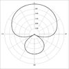
Supercardioid -
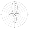
Shotgun


Some microphone designs combine several principles in creating the desired polar pattern. This ranges from shielding (meaning diffraction/dissipation/absorption) by the housing itself to electronically combining dual membranes.
Omnidirectional
An omnidirectional (or nondirectional) microphone's response is generally considered to be a perfect sphere in three dimensions. In the real world, this is not the case. As with directional microphones, the polar pattern for an "omnidirectional" microphone is a function of frequency. The body of the microphone is not infinitely small and, as a consequence, it tends to get in its own way with respect to sounds arriving from the rear, causing a slight flattening of the polar response. This flattening increases as the diameter of the microphone (assuming it's cylindrical) reaches the wavelength of the frequency in question. Therefore, the smallest diameter microphone gives the best omnidirectional characteristics at high frequencies.The wavelength of sound at 10 kHz is 1.4" (3.5 cm). The smallest measuring microphones are often 1/4" (6 mm) in diameter, which practically eliminates directionality even up to the highest frequencies. Omnidirectional microphones, unlike cardioids, do not employ resonant cavities as delays, and so can be considered the "purest" microphones in terms of low coloration; they add very little to the original sound. Being pressure-sensitive they can also have a very flat low-frequency response down to 20 Hz or below. Pressure-sensitive microphones also respond much less to wind noise and plosives than directional (velocity sensitive) microphones.
An example of a nondirectional microphone is the round black eight ball.
Unidirectional
A unidirectional microphone is primarily sensitive to sounds from only one direction. The diagram above illustrates a number of these patterns. The microphone faces upwards in each diagram. The sound intensity for a particular frequency is plotted for angles radially from 0 to 360°. (Professional diagrams show these scales and include multiple plots at different frequencies. The diagrams given here provide only an overview of typical pattern shapes, and their names.)Cardioid, Hypercardioid, Supercardioid

University Sound US664A dynamic supercardioid microphone
A cardioid microphone is effectively a superposition of an omnidirectional and a figure-8 microphone; for sound waves coming from the back, the negative signal from the figure-8 cancels the positive signal from the omnidirectional element, whereas for sound waves coming from the front, the two add to each other. A hyper-cardioid microphone is similar, but with a slightly larger figure-8 contribution leading to a tighter area of front sensitivity and a smaller lobe of rear sensitivity. A super-cardioid microphone is similar to a hyper-cardioid, except there is more front pickup and less rear pickup. While any pattern between omni and figure 8 is possible by adjusting their mix, common definitions state that a hypercardioid is produced by combining them at a 3:1 ratio, producing nulls at 109.5°, while supercardioid is produced with a 5:3 ratio, with nulls at 126.9°.
Bi-directional
"Figure 8" or bi-directional microphones receive sound equally from both the front and back of the element. Most ribbon microphones are of this pattern. In principle they do not respond to sound pressure at all, only to the change in pressure between front and back; since sound arriving from the side reaches front and back equally there is no difference in pressure and therefore no sensitivity to sound from that direction. In more mathematical terms, while omnidirectional microphones are scalar transducers responding to pressure from any direction, bi-directional microphones are vector transducers responding to the gradient along an axis normal to the plane of the diaphragm. This also has the effect of inverting the output polarity for sounds arriving from the back side.Shotgun and parabolic microphones

An Audio-Technica shotgun microphone

The interference tube of a shotgun microphone. The capsule is at the base of the tube.

A Sony parabolic reflector, without a microphone. The microphone would
face the reflector surface and sound captured by the reflector would
bounce towards the microphone.
Boundary or "PZM"
Several approaches have been developed for effectively using a microphone in less-than-ideal acoustic spaces, which often suffer from excessive reflections from one or more of the surfaces (boundaries) that make up the space. If the microphone is placed in, or very close to, one of these boundaries, the reflections from that surface have the same timing as the direct sound, thus giving the microphone a hemispherical polar pattern and improved intelligibility. Initially this was done by placing an ordinary microphone adjacent to the surface, sometimes in a block of acoustically transparent foam. Sound engineers Ed Long and Ron Wickersham developed the concept of placing the diaphragm parallel to and facing the boundary. While the patent has expired, "Pressure Zone Microphone" and "PZM" are still active trademarks of Crown International, and the generic term "boundary microphone" is preferred. While a boundary microphone was initially implemented using an omnidirectional element, it is also possible to mount a directional microphone close enough to the surface to gain some of the benefits of this technique while retaining the directional properties of the element. Crown's trademark on this approach is "Phase Coherent Cardioid" or "PCC," but there are other makers who employ this technique as well.Application-specific designs
A lavalier microphone is made for hands-free operation. These small microphones are worn on the body. Originally, they were held in place with a lanyard worn around the neck, but more often they are fastened to clothing with a clip, pin, tape or magnet. The lavalier cord may be hidden by clothes and either run to an RF transmitter in a pocket or clipped to a belt (for mobile use), or run directly to the mixer (for stationary applications).A wireless microphone transmits the audio as a radio or optical signal rather than via a cable. It usually sends its signal using a small FM radio transmitter to a nearby receiver connected to the sound system, but it can also use infrared waves if the transmitter and receiver are within sight of each other.
A contact microphone picks up vibrations directly from a solid surface or object, as opposed to sound vibrations carried through air. One use for this is to detect sounds of a very low level, such as those from small objects or insects. The microphone commonly consists of a magnetic (moving coil) transducer, contact plate and contact pin. The contact plate is placed directly on the vibrating part of a musical instrument or other surface, and the contact pin transfers vibrations to the coil. Contact microphones have been used to pick up the sound of a snail's heartbeat and the footsteps of ants. A portable version of this microphone has recently been developed. A throat microphone is a variant of the contact microphone that picks up speech directly from a person's throat, which it is strapped to. This lets the device be used in areas with ambient sounds that would otherwise make the speaker inaudible.
A parabolic microphone uses a parabolic reflector to collect and focus sound waves onto a microphone receiver, in much the same way that a parabolic antenna (e.g. satellite dish) does with radio waves. Typical uses of this microphone, which has unusually focused front sensitivity and can pick up sounds from many meters away, include nature recording, outdoor sporting events, eavesdropping, law enforcement, and even espionage. Parabolic microphones are not typically used for standard recording applications, because they tend to have poor low-frequency response as a side effect of their design.
A stereo microphone integrates two microphones in one unit to produce a stereophonic signal. A stereo microphone is often used for broadcast applications or field recording where it would be impractical to configure two separate condenser microphones in a classic X-Y configuration (see microphone practice) for stereophonic recording. Some such microphones have an adjustable angle of coverage between the two channels.
A noise-canceling microphone is a highly directional design intended for noisy environments. One such use is in aircraft cockpits where they are normally installed as boom microphones on headsets. Another use is in live event support on loud concert stages for vocalists involved with live performances. Many noise-canceling microphones combine signals received from two diaphragms that are in opposite electrical polarity or are processed electronically. In dual diaphragm designs, the main diaphragm is mounted closest to the intended source and the second is positioned farther away from the source so that it can pick up environmental sounds to be subtracted from the main diaphragm's signal. After the two signals have been combined, sounds other than the intended source are greatly reduced, substantially increasing intelligibility. Other noise-canceling designs use one diaphragm that is affected by ports open to the sides and rear of the microphone, with the sum being a 16 dB rejection of sounds that are farther away. One noise-canceling headset design using a single diaphragm has been used prominently by vocal artists such as Garth Brooks and Janet Jackson. A few noise-canceling microphones are throat microphones.
Powering
Microphones containing active circuitry, such as most condenser microphones, require power to operate the active components. The first of these used vacuum-tube circuits with a separate power supply unit, using a multi-pin cable and connector. With the advent of solid-state amplification, the power requirements were greatly reduced and it became practical to use the same cable conductors and connector for audio and power. During the 1960s several powering methods were developed, mainly in Europe. The two dominant methods were initially defined in German DIN 45595 as de:Tonaderspeisung or T-power and DIN 45596 for phantom power. Since the 1980s, phantom power has become much more common, because the same input may be used for both powered and unpowered microphones. In consumer electronics such as DSLRs and camcorders, "plug-in power" is more common, for microphones using a 3.5 mm phone plug connector. Phantom, T-power and plug-in power are described in international standard IEC 61938.Connectors

Electronic symbol for a microphone
- Male XLR connector on professional microphones
- ¼ inch (sometimes referred to as 6.3 mm) phone connector on less expensive musician's microphones, using an unbalanced 1/4 inch (6.3 mm) TS phone connector. Harmonica microphones commonly use a high impedance 1/4 inch (6.3 mm) TS connection to be run through guitar amplifiers.
- 3.5 mm (sometimes referred to as 1/8 inch mini) stereo (sometimes wired as mono) mini phone plug on prosumer camera, recorder and computer microphones.

A microphone with a USB connector, made by Blue Microphones
Impedance-matching
|
|
This section's factual accuracy is disputed. (September 2015) |
The output of a given microphone delivers the same power whether it is low or high impedance[citation needed]. If a microphone is made in high and low impedance versions, the high impedance version has a higher output voltage for a given sound pressure input, and is suitable for use with vacuum-tube guitar amplifiers, for instance, which have a high input impedance and require a relatively high signal input voltage to overcome the tubes' inherent noise. Most professional microphones are low impedance, about 200 Ω or lower. Professional vacuum-tube sound equipment incorporates a transformer that steps up the impedance of the microphone circuit to the high impedance and voltage needed to drive the input tube. External matching transformers are also available that can be used in-line between a low impedance microphone and a high impedance input.
Low-impedance microphones are preferred over high impedance for two reasons: one is that using a high-impedance microphone with a long cable results in high frequency signal loss due to cable capacitance, which forms a low-pass filter with the microphone output impedance[citation needed]. The other is that long high-impedance cables tend to pick up more hum (and possibly radio-frequency interference (RFI) as well). Nothing is damaged if the impedance between microphone and other equipment is mismatched; the worst that happens is a reduction in signal or change in frequency response.
Some microphones are designed not to have their impedance matched by the load they are connected to.Doing so can alter their frequency response and cause distortion, especially at high sound pressure levels. Certain ribbon and dynamic microphones are exceptions, due to the designers' assumption of a certain load impedance being part of the internal electro-acoustical damping circuit of the microphone.
Digital microphone interface

Neumann D-01 digital microphone and Neumann DMI-8 8-channel USB Digital Microphone Interface
Measurements and specifications

A comparison of the far field on-axis frequency response of the Oktava 319 and the Shure SM58
A frequency response diagram plots the microphone sensitivity in decibels over a range of frequencies (typically 20 Hz to 20 kHz), generally for perfectly on-axis sound (sound arriving at 0° to the capsule). Frequency response may be less informatively stated textually like so: "30 Hz–16 kHz ±3 dB". This is interpreted as meaning a nearly flat, linear, plot between the stated frequencies, with variations in amplitude of no more than plus or minus 3 dB. However, one cannot determine from this information how smooth the variations are, nor in what parts of the spectrum they occur. Note that commonly made statements such as "20 Hz–20 kHz" are meaningless without a decibel measure of tolerance. Directional microphones' frequency response varies greatly with distance from the sound source, and with the geometry of the sound source. IEC 60268-4 specifies that frequency response should be measured in plane progressive wave conditions (very far away from the source) but this is seldom practical. Close talking microphones may be measured with different sound sources and distances, but there is no standard and therefore no way to compare data from different models unless the measurement technique is described.
The self-noise or equivalent input noise level is the sound level that creates the same output voltage as the microphone does in the absence of sound. This represents the lowest point of the microphone's dynamic range, and is particularly important should you wish to record sounds that are quiet. The measure is often stated in dB(A), which is the equivalent loudness of the noise on a decibel scale frequency-weighted for how the ear hears, for example: "15 dBA SPL" (SPL means sound pressure level relative to 20 micropascals). The lower the number the better. Some microphone manufacturers state the noise level using ITU-R 468 noise weighting, which more accurately represents the way we hear noise, but gives a figure some 11–14 dB higher. A quiet microphone typically measures 20 dBA SPL or 32 dB SPL 468-weighted. Very quiet microphones have existed for years for special applications, such the Brüel & Kjaer 4179, with a noise level around 0 dB SPL. Recently some microphones with low noise specifications have been introduced in the studio/entertainment market, such as models from Neumann and Røde that advertise noise levels between 5–7 dBA. Typically this is achieved by altering the frequency response of the capsule and electronics to result in lower noise within the A-weighting curve while broadband noise may be increased.
The maximum SPL the microphone can accept is measured for particular values of total harmonic distortion (THD), typically 0.5%. This amount of distortion is generally inaudible,[citation needed] so one can safely use the microphone at this SPL without harming the recording. Example: "142 dB SPL peak (at 0.5% THD)". The higher the value, the better, although microphones with a very high maximum SPL also have a higher self-noise.
The clipping level is an important indicator of maximum usable level, as the 1% THD figure usually quoted under max SPL is really a very mild level of distortion, quite inaudible especially on brief high peaks. Clipping is much more audible. For some microphones the clipping level may be much higher than the max SPL.
The dynamic range of a microphone is the difference in SPL between the noise floor and the maximum SPL. If stated on its own, for example "120 dB", it conveys significantly less information than having the self-noise and maximum SPL figures individually.
Sensitivity indicates how well the microphone converts acoustic pressure to output voltage. A high sensitivity microphone creates more voltage and so needs less amplification at the mixer or recording device. This is a practical concern but is not directly an indication of the microphone's quality, and in fact the term sensitivity is something of a misnomer, "transduction gain" being perhaps more meaningful, (or just "output level") because true sensitivity is generally set by the noise floor, and too much "sensitivity" in terms of output level compromises the clipping level. There are two common measures. The (preferred) international standard is made in millivolts per pascal at 1 kHz. A higher value indicates greater sensitivity. The older American method is referred to a 1 V/Pa standard and measured in plain decibels, resulting in a negative value. Again, a higher value indicates greater sensitivity, so −60 dB is more sensitive than −70 dB.
Measurement microphones
Some microphones are intended for testing speakers, measuring noise levels and otherwise quantifying an acoustic experience. These are calibrated transducers and are usually supplied with a calibration certificate that states absolute sensitivity against frequency. The quality of measurement microphones is often referred to using the designations "Class 1," "Type 2" etc., which are references not to microphone specifications but to sound level meters.[49] A more comprehensive standard[50] for the description of measurement microphone performance was recently adopted.Measurement microphones are generally scalar sensors of pressure; they exhibit an omnidirectional response, limited only by the scattering profile of their physical dimensions. Sound intensity or sound power measurements require pressure-gradient measurements, which are typically made using arrays of at least two microphones, or with hot-wire anemometers.
Microphone calibration
Main article: Measurement microphone calibration
To take a scientific measurement with a microphone, its precise sensitivity must be known (in volts per pascal). Since this may change over the lifetime of the device, it is necessary to regularly calibrate
measurement microphones. This service is offered by some microphone
manufacturers and by independent certified testing labs. All microphone calibration is ultimately traceable to primary standards at a national measurement institute such as NPL in the UK, PTB in Germany and NIST
in the United States, which most commonly calibrate using the
reciprocity primary standard. Measurement microphones calibrated using
this method can then be used to calibrate other microphones using
comparison calibration techniques.Depending on the application, measurement microphones must be tested periodically (every year or several months, typically) and after any potentially damaging event, such as being dropped (most such microphones come in foam-padded cases to reduce this risk) or exposed to sounds beyond the acceptable level.
Microphone array and array microphones
Main article: Microphone array
A microphone array is any number of microphones operating in tandem. There are many applications:- Systems for extracting voice input from ambient noise (notably telephones, speech recognition systems, hearing aids)
- Surround sound and related technologies
- Locating objects by sound: acoustic source localization, e.g., military use to locate the source(s) of artillery fire. Aircraft location and tracking.
- High fidelity original recordings
- 3D spatial beamforming for localized acoustic detection of subcutaneous sounds
Microphone windscreens

Microphone with its windscreen removed.
See also: Pop filter
Windscreens (or windshields – the terms are interchangeable)
provide a method of reducing the effect of wind on microphones. While
pop-screens give protection from unidirectional blasts, foam “hats”
shield wind into the grille from all directions, and blimps / zeppelins /
baskets entirely enclose the microphone and protect its body as well.
This last point is important because, given the extreme low frequency
content of wind noise, vibration induced in the housing of the
microphone can contribute substantially to the noise output.
The shielding material used – wire gauze, fabric or foam – is designed to have a significant acoustic impedance. The relatively low particle-velocity air pressure changes that constitute sound waves can pass through with minimal attenuation, but higher particle-velocity wind is impeded to a far greater extent. Increasing the thickness of the material improves wind attenuation but also begins to compromise high frequency audio content. This limits the practical size of simple foam screens. While foams and wire meshes can be partly or wholly self-supporting, soft fabrics and gauzes require stretching on frames, or laminating with coarser structural elements.
Since all wind noise is generated at the first surface the air hits, the greater the spacing between shield periphery and microphone capsule, the greater the noise attenuation. For an approximately spherical shield, attenuation increases by (approximately) the cube of that distance. Thus larger shields are always much more efficient than smaller ones. With full basket windshields there is an additional pressure chamber effect, first explained by Joerg Wuttke, which, for two-port (pressure gradient) microphones, allows the shield/microphone combination to act as a high-pass acoustic filter.
Since turbulence at a surface is the source of wind noise, reducing gross turbulence can add to noise reduction. Both aerodynamically smooth surfaces, and ones that prevent powerful vortices being generated, have been used successfully. Historically, artificial fur has proved very useful for this purpose since the fibres produce micro-turbulence and absorb energy silently. If not matted by wind and rain, the fur fibres are very transparent acoustically, but the woven or knitted backing can give significant attenuation. As a material it suffers from being difficult to manufacture with consistency, and to keep in pristine condition on location. Thus there is an interest (DPA 5100, Rycote Cyclone) to move away from its use.
In the studio and on stage, pop-screens and foam shields can be useful for reasons of hygiene, and protecting microphones from spittle and sweat. They can also be useful coloured idents. On location the basket shield can contain a suspension system to isolate the microphone from shock and handling noise.
Stating the efficiency of wind noise reduction is an inexact science, since the effect varies enormously with frequency, and hence with the bandwidth of the microphone and audio channel. At very low frequencies (10–100 Hz) where massive wind energy exists, reductions are important to avoid overloading of the audio chain – particularly the early stages. This can produce the typical “wumping” sound associated with wind, which is often syllabic muting of the audio due to LF peak limiting. At higher frequencies – 200 Hz to ~3 kHz – the aural sensitivity curve allows us to hear the effect of wind as an addition to the normal noise floor, even though it has a far lower energy content. Simple shields may allow the wind noise to be 10 dB less apparent; better ones can achieve nearer to a 50 dB reduction. However the acoustic transparency, particularly at HF, should also be indicated, since a very high level of wind attenuation could be associated with very muffled audio.
-
 Various microphone covers
-
 Two recordings being made—a blimp is being used on the left. An open-cell foam windscreen is being used on the right.
-
 "Dead cat" and a "dead kitten" windscreens. The dead kitten covers a stereo microphone for a DSLR camera. The difference in name is due to the size of the fur.


