NOVEMBER 2019


Real-Time mean
“Real-time” essentially means “happening now or immediately responsive.” In engineering, real-time refers to systems that not only need to calculate the correct response, but they must respond instantly, often in continuous interaction (dynamically) with the system’s environment.
Real-time is an expression used in two main areas with respect to software and electronics. Real-time can refer to a clock in a circuit, as in a Real Time Clock (RTC). An RTC is a circuit that tracks time and date, and is used for setting alarms in relation to time and calendar. An RTC has to remain energized in order to maintain the current time and date; otherwise, the time and date must be reset. An RTC cannot recover the time once it’s lost track of it; not without some form of power to run it. Thus, many RTCs are designed with a trickle of power or a battery, even if everything else has “gone to sleep” to preserve power. An RTC should not be confused with the “clock” or “timer” in a circuit with an MCU. A clock or timer performs a very different function of timing (or clocking) computational cycles for a processor or controller.
The term “real-time” is also used with computers and controllers. Here, real-time refers to the immediacy of response that the “brain” of the device handles. A processor, controller, or operating system is real-time if it is able to respond immediately to situations without waiting for an hour glass icon to stop turning. Personal computers (PCs) are not meant to run real-time processes in this sense and do not have real-time operating systems; i.e., Windows and iOS operating systems are not meant for the often critical capability required of real-time systems. They do, however, have an RTC so that they can keep calendars and reminders.
Real-time control is critical in many applications due to safety issues. Examples of applications that have real-time constraints are the automotive industry (e.g., drive-by-wire and ABS), air traffic control, process controls, and medical devices (e.g., a pacemaker).

Real-time control or computing requires the processor to prioritize interrupts as they come in and act immediately on those of higher priority, and in “hard” cases without first finishing the task that is currently occupying the processor. “Hard” real-time cannot be dependent on anything that is not 100% reliable in turn, because an event that requires a real-time response cannot wait for an internet connection, for instance. Hard real-time refers to the fact that there are fatal consequences if the system fails to respond in time. In contrast, “soft real-time” is more tolerant of a missed deadline, but the consequences are still not favorable. The lateness of the response affects the value of the deliverable. With hard real-time systems, a late delivery is the same as no delivery at all.
In another example, a soft real-time system may wait for failure before taking corrective action, like a skipped spot on a DVD. A hard real-time system, however, may need to calculate that a good outcome is possible with a given task before performing it. Otherwise, it might perform a different task based on calculations that the deadline cannot be met with the initial, default task. Real-time systems need predictable, dependable resources, especially if there are dynamic inputs and processes that are required for successful execution.

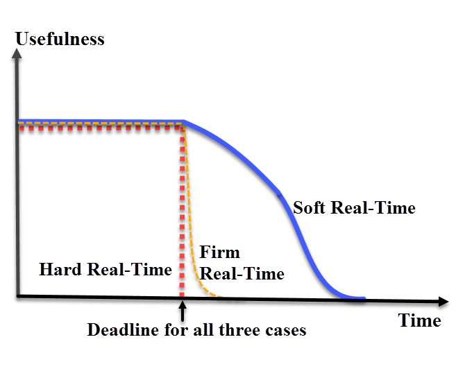
Figure
1: Hard real-time processes require an immediate response to have any
value. Firm or near real-time processes have quickly decreasing value
after a missed deadline, whereas soft real-time decreases in usefulness
over a longer period.
“Firm” real-time is a less-often used term, but like near real-time, it indicates that it is not soft real-time, but not hard real-time, either. A near/firm real-time system might infrequently miss a deadline and cause failure that is not catastrophic, but can be catastrophic if multiple deadlines are missed. An example of a firm real-time system is an automotive robot that occasionally misses a rivet weld. QA personnel downstream can still catch this failure and spot weld it, but missing many welds or missing them randomly and often can ruin the synchronization of the entire production line or cause total failure if the fault is missed. Getting to hard real-time involves more time and effort with exercises such as a Failure Mode Effect Analysis (FMEA) for hard real-time systems.
The study of real-time systems is wide-spread as it applies to aerospace, military, medical, computing, financial and many other industries. Fault tolerant computing is another area where real-time is an important topic; a single failure can lead to a catastrophic system failure. Quality of Service (QoS) is another area within networking where the concept of real-time is relevant, because poor QoS can lead to customer desertion, among other things.
_________________________________________________________________________________
Difference Between Hard and Soft Real Time System
Key Difference – Hard vs Soft Real Time System
The key difference between hard and soft real time system is that, a
hard-real time system is a system in which a single failure to meet the
deadline may lead to a complete system failure while a soft real time
system is a system in which one or more failures to meet the deadline is
not considered as complete system failure, but its performance is
considered degraded.
An operating system is a system software
that manages the computer hardware according to the instructions
provided by the software. An operating system provides various tasks.
File management, memory management, controlling peripheral devices and
process scheduling are some of them. One type of an operating system is a
real time operating system. It can be divided into hard real time
systems and soft real time systems.
What is Hard Real Time System?
A real time system is a data processing
system. The time taken by the system to respond to an input and provide
the output or display the updated information is known as the response
time. So, in these systems, the response time should be very minimum.
The system should complete the task within the deadline. In a real-time
operating system, the correctness of the system output depends on the
logical result of computation as well as the time it takes to produce
the result. Their systems also have a structure similar to an ordinary
operating system. It also has mechanisms for real time scheduling tasks.
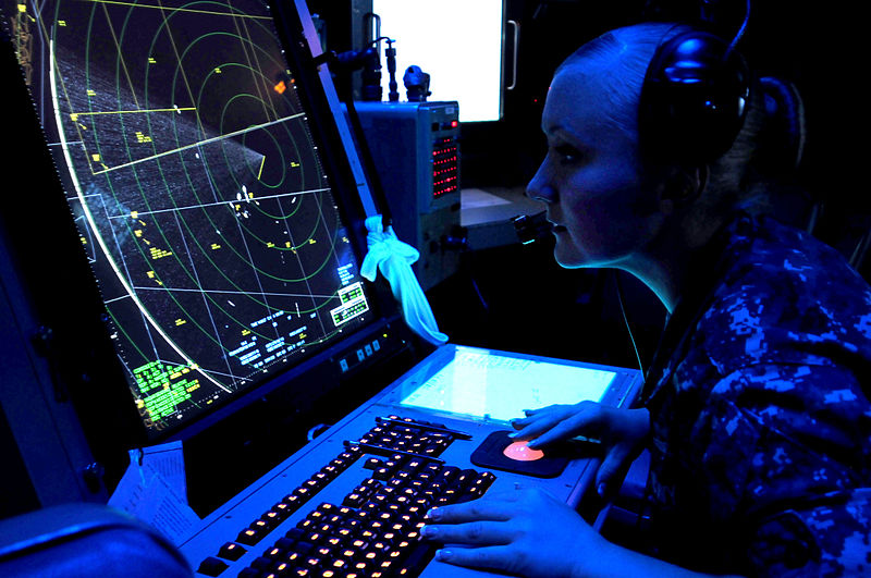
Figure 01: Air Traffic Control System
In hard real time system, the time
requirement is a critical constraint. The system should perform within
the deadline. If the system didn’t perform within the deadline, it is
considered as a task failure. These types of systems should not miss the
deadline. Missing the deadline can be catastrophic. Air traffic control
systems, missile, and nuclear reactor control systems are few examples
for hard real time systems. If the aircraft control system didn’t give
the instructions to the aircraft within the deadline, it can cause the
air craft to crash. Therefore, in a hard-real time system, meeting the
deadline is extremely important. These systems are deployed mainly into
safety critical systems.
What is Soft Real Time System?
In a soft real time, system, the time
requirement is not very crucial. The system should perform the task or
give the output within the deadline but there can be a small tolerance
occasionally. If the system, did not perform the task within the
deadline it is not considered as a failure as long as it provides the
required output. But performance is considered to be degraded. Missing
the deadline will not cause a catastrophic event like in a hard-real
time system. These systems are less restrictive. Some examples of
software real-time systems are multimedia streaming, advanced scientific
projects, and virtual reality.
What is the Difference Between Hard and Soft Real Time System?
Hard vs Soft Real Time System |
|
| A hard-real time system is a system in which a failure to meet even a single deadline may lead to complete or catastrophic system failure. | A soft real time system is a system in which one or more failures to meet the deadline is not considered as complete system failure but that performance is considered to be degraded. |
| Restrictive Nature | |
| A Hard-real time system is very restrictive. | A Soft real time system is not very restrictive. |
| Deadline | |
| A Hard-real time system should not miss the deadline. Missing the deadline cause complete or catastrophic system failure. | A Soft real time system can miss the deadline occasionally. Missing the deadline is not considered as a complete system failure but degrades the performance. |
| Utility | |
| A hard-real time system has more utility. | A soft real time system has less utility. |
| Examples | |
| Air traffic control systems, missile, and nuclear reactor control systems are some examples of hard real time systems. | Multimedia streaming, advanced scientific projects, and virtual reality are some examples of soft real time systems. |
Summary – Hard vs Soft Real Time System
This article discussed two types of real
time operating systems; the hard real time systems and the soft real
time systems. The difference between hard and soft real time system is
that, a hard-real time system is a system in which a single failure to
meet the deadline may lead to a complete system failure while a soft
real time system is a system in which one or more failures to meet the
deadline is not considered as complete system failure but its
performance is considered degraded.
__________________________________________________________________________________
Deadline Scheduling for Real-Time Systems
Real-time systems are
all around us. They are in our home appliances, banking ATM's, cash
registers, and even in trains, planes, and automobiles. Real-time
systems outnumber all other types of computers. This lesson provides a
detailed look at how real-time systems schedule the tasks that control
our world.
Introduction to Real-Time Systems
Real-time systems (RTS) are carefully designed systems consisting of software and hardware used to capture and respond to events occurring in the real world. Like many computer systems, the RTS process must operate correctly, but it has an additional requirement in that it must act in a timely manner. If an automobile's RTS controlling your brakes do not act in a timely manner, it may cause a catastrophic event. To accomplish this goal, the design engineer must carefully select from a variety of real-time scheduling options available. Let's define what we mean by a process and look at a few of the process properties illustrated in Figure 1. |
The Real-time System Process
The RTS process is computer code that is executed as the result of a detected or scheduled event. It is intentionally kept small so it can be executed very quickly to allow other processes to be scheduled and executed. Some of the characteristics of the process are shown and explained Figure 1.Real-Time System Configurations, Events, and Scheduling
There are multiple configurations, events, and scheduling types that are associated with the real-time process. A flow of these configurations and events are outlined in Figure 2 and expounded upon in the following sections. |
Hard and Soft Real-time
A real-time system can be characterized as a soft or hard system. Soft real-time systems may miss some deadlines, but performance may degrade if too many are missed. Examples of soft real-time systems are household appliances, portable MP3 players, and entertainment systems. A hard-real-time system must never miss a deadline or it may cause a catastrophic event. Hard real-time systems may be used to control aircraft, power plants and your family car.Periodic, Aperiodic and Sporadic Events
The hardware of an RTS detects events that occur in the real world. These events can be periodic, aperiodic or sporadic. Periodic events repeat in regular intervals. An aperiodic event can happen just once or it may occur multiple times over time. Sporadic events can appear very often, but not in a constant or regular manner.Static and Dynamic Scheduling
Static Scheduling is the where the system designer has analyzed the characteristics of each process and specified the exact order of process execution. During execution of the RTS, the order of the scheduled processes will not change.Dynamic Scheduling is the mechanism where thread scheduling is done by the RTS based on a selected scheduling algorithm. The execution order of threads is completely controlled by that algorithm. During execution of the RTS, the order of the scheduled processes will constantly change.
Preemptive, Non-Preemptive and Mixed Scheduling
The scheduling algorithm you choose depends on your project. Different algorithms can yield different results. Projects can differ in the number of processes needed, and the process response time, priorities and deadlines. The scheduling algorithm must guarantee all critical timing constraints are met.Some real-time systems use preemptive scheduling. In this type of scheduling system, the process priorities are assigned. The RTS always executes the process with the highest priority first. Lower priority processes can be interrupted in the middle of execution to allow a higher priority process to execute. Once the higher priority process completes execution, the lower priority process can then continue execution from the point where it was interrupted. In a non-preemptive scheduling system, once a process starts execution it is never interrupted by another process. There are some scheduling systems that use mixed scheduling. In this type of scheduling, there are high priority processes that are non-preemptive and lower priority processes that are preemptive.
Single and Multiple Processors
For some of the smaller real-time systems, a single processor computer system is used. On more complex systems, multiple processors are used so processes can be assigned to different processors to make sure they all can meet their deadlines.Real-Time Scheduling
Real-time systems can be very simple or they can be very complex to implement. Another factor that can be very important is criticality. Will the failure of an RTS cause the loss of like, or large financial loss? These factors play a role in how you design an RTS.The table in Figure 3 outlines a matrix of different RTS configurations.
 |
_________________________________________________________________________________
The Importance of Metrics and Operating Systems
Latency is an important practical concern in the robotics world that is often poorly understood. I feel that a better understanding of latency can help robotics researchers and engineers make design and architecture decisions that greatly streamline and accelerate the R&D process. I’ve personally spent many hours looking for information on the latency characteristics of various robotic components, but have had difficulty finding anything that is clearly presented or backed by solid data. From what I’ve found, most benchmarks focus on the maximum throughput and either ignore the subject of latency or measure it incorrectly.
two main topics in latency :
-
The details of how you measure latency matters.
-
The OS that you use affects your latency.
Measuring Latency
Robots are controlled in real-time, which means that a command gets executed within a deadline (fixed period of time). There are hard real-time systems that must never exceed their deadline, and soft real-time
systems that are able to occasionally exceed their deadline. Missing
deadlines when performing motor control of a robot can result in
unwanted motions and 'jerky' behavior.
Although there is a lot of information on the theoretical definition
of these terms, it can be challenging to determine the maximum deadline
(point at which a system’s performance starts to degrade or become
unsafe) for practical applications. This is especially true for research
institutions that build novel mechanisms and target cutting-edge
applications. Many research groups end up assuming that everything needs
to be hard real-time with very stringent deadlines. While this approach
provides solid performance guarantees, it can also create a lot of
unnecessary development overhead.
Many benchmarks and tools make the assumption that latency follows a Gaussian distribution and report only the mean and the standard deviation. Unfortunately, latency tends to be very multi-modal
and the most important part of the distribution when it comes to
determinism are the 'outliers'. Even if a system’s latency behaves as
expected in 99% of the cases, the leftover 1% can be worse than all of
the other 99% of measurements combined. Looking at only the mean and
standard deviation completely fails to capture the more systemic issues.
For example, I’ve seen many data sets where the worst observed case was
more than 1000 standard deviations away from the mean. Such stutters
are usually the main problem when working on real robotic systems.
Because of this, a more appropriate way to look at latency is via histograms and percentile plots, e.g., "99.9% of measurements were below X ms". There are several good resources about recording latency out there .
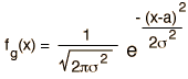
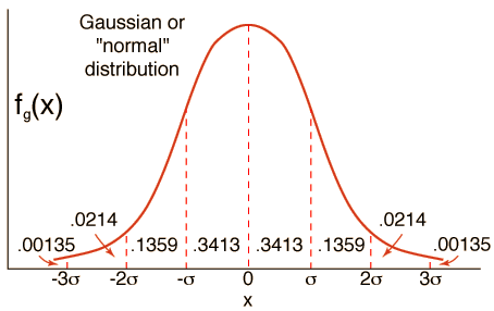
If the number of events is very large, then the Gaussian distribution function may be used to describe physical events. The Gaussian distribution is a continuous function which approximates the exact binomial distribution of events.
The Gaussian distribution shown is normalized so that the sum over all values of x gives a probability of 1. The nature of the gaussian gives a probability of 0.683 of being within one standard deviation of the mean. The mean value is a=np where n is the number of events and p the probability of any integer value of x (this expression carries over from the binomial distribution ). The standard deviation expression used is also that of the binomial distribution.
The Gaussian distribution is also commonly called the "normal distribution" and is often described as a "bell-shaped curve".
Gaussian Distribution Function
| Distribution | Functional Form | Mean | Standard Deviation |
| Gaussian |  |  |  |
| Distribution | Functional Form | Mean | Standard Deviation |
| Gaussian | |  |  |
If the number of events is very large, then the Gaussian distribution function may be used to describe physical events. The Gaussian distribution is a continuous function which approximates the exact binomial distribution of events.
The Gaussian distribution shown is normalized so that the sum over all values of x gives a probability of 1. The nature of the gaussian gives a probability of 0.683 of being within one standard deviation of the mean. The mean value is a=np where n is the number of events and p the probability of any integer value of x (this expression carries over from the binomial distribution ). The standard deviation expression used is also that of the binomial distribution.
The Gaussian distribution is also commonly called the "normal distribution" and is often described as a "bell-shaped curve".
Gaussian distribution is the distribution of data and behavior that may be the most correct and best for the logic of data distribution and dynamic motion information whose position is in the middle and most likely or data that does not undergo refraction and normal distribution of program conditions is probably the most appropriate and stable for a long period of time .
Gamma Function territory of Gaussian distribution
Hyper Physics
Rationale for Development
Hyper Physics is an exploration environment for concepts in physics which employs concept maps and other linking strategies to facilitate smooth navigation. For the most part, it is laid out in small segments or "cards", true to its original development in Hyper Card. The entire environment is interconnected with thousands of links, reminiscent of a neural network. The bottom bar of each card contains links to major concept maps for divisions of physics, plus a "go back" feature to allow you to retrace the path of an exploration.
Operating Systems ( Software ++ Hardware )
The operating system is at the base of everything. No matter how
performant the high-level software stack is, the system is fundamentally
bound by the capabilities of the OS, it’s scheduler, and the overall
load on the system. Before you start optimizing your own software, you
should make sure that your goal is actually achievable on the underlying
platform.
There are trade-offs between always responding in a timely manner and
overall performance, battery life, as well as several other concerns.
Because of this, the major consumer operating systems don’t guarantee to
meet hard deadlines and can theoretically have arbitrarily long pauses.
However, since using operating systems that users are familiar with
can significantly ease development, it is worth evaluating their actual
performance and capabilities. Even though there may not be any
theoretical guarantees, the practical differences are often not
noticeable.
Developing hard real-time systems has a lot of pitfalls and can require a lot of development effort. Windows / Mac / Linux is OS in this world this now
Dexterity + mobility = autonomy
Digital logic for soft devices
Soft devices offer many useful characteristics, including safe operation in close proximity to humans, the ability to adapt to their surroundings, ease of sterilization, simplicity, low cost, and light weight. Current soft devices, however, are still actuated by hard valves and electronic controls, and reliance on these components limits the use of soft devices in applications where hard structures or electronics are not compatible. This work demonstrates completely soft digital logic gates that can be integrated into soft devices and that allow computation and control within these devices, without hard valves or electronics. We demonstrate data storage, signal processing, digital-to-analog conversion, environmental sensing, and collaborative interaction between humans and soft devices.
Although soft devices (grippers, actuators, and elementary robots) are rapidly becoming an integral part of the broad field of robotics, autonomy for completely soft devices has only begun to be developed. Adaptation of conventional systems of control to soft devices requires hard valves and electronic controls. This paper describes completely soft pneumatic digital logic gates having a physical scale appropriate for use with current (macroscopic) soft actuators. Each digital logic gate utilizes a single bi stable valve—the pneumatic equivalent of a Schmitt trigger—which relies on the snap-through instability of a hemispherical membrane to kink internal tubes and operates with binary high/low input and output pressures. Soft, pneumatic NOT, AND, and OR digital logic gates—which generate known pneumatic outputs as a function of one, or multiple, pneumatic inputs—allow fabrication of digital logic circuits for a set–reset latch, two-bit shift register, leading-edge detector, digital-to-analog converter (DAC), and toggle switch. The DAC and toggle switch, in turn, can control and power a soft actuator (demonstrated using a pneu-net gripper). These macroscale soft digital logic gates are scalable to high volumes of airflow, do not consume power at steady state, and can be reconfigured to achieve multiple functionalities from a single design (including configurations that receive inputs from the environment and from human users). This work represents a step toward a strategy to develop autonomous control—one not involving an electronic interface or hard components—for soft devices. More “intelligent” control—for example, control based on digital logic and computation .
Schmitt Trigger Hysteresis Electronic Circuit Comparator ...

++++++++++++++++++++++++++++++++++++++++++++++++++++++++++++++++++++++++
In
an application for which the applied force is important, the robot
needs to be controlled differently. Instead of servoing each joint to
its targeted position, the output torque is controlled to match the
desired force applied by the end-effector on an external object. To do
this, a way of measuring the external force is required.
Force/Torque Sensors
Typically, the external force is measured using a six-axis force/torque sensor which measures any force applied to the end-effector. Most of the commercially available force/torque sensors are built from strain gages. Some robot manufacturers offer force-control packages containing the sensor, plus a special software, which allows you to program the robot using force control.Sensorless Force Control
One question begs to be asked at this point: is it possible to control the applied force using a normal, position-controlled robot? Well, the answer is yes, but not directly. One way to do this is by having a compliant end-effector for which the relation between displacement and force is well-known. Instead of controlling the force, the position trajectory is programmed to control the deformation of the tool in order to match the desired applied force. This approach is more simple but has some disadvantages: the position of the object has to be known precisely, the contact surface has to be stiff and the end-effector has to be compliant in only one direction. If one of these assumptions is not met, the results are often compromised. Therefore, a force/torque sensor is the best option to obtain precision in force control.Force Control Basics
 At first glance, the basic idea behind force control is simple: the
output of the sensor is used to close the loop in the controller,
adjusting each of the joint torque to match the desired output. In a
certain way, this is similar to position control. You simply replace the
reference position (from the motor encoders) by a reference force (from
the force/torque sensor).
At first glance, the basic idea behind force control is simple: the
output of the sensor is used to close the loop in the controller,
adjusting each of the joint torque to match the desired output. In a
certain way, this is similar to position control. You simply replace the
reference position (from the motor encoders) by a reference force (from
the force/torque sensor).Unfortunately, it is not always as easy as that. The problems come from the fact that the robot needs to perform a trajectory in certain directions while a precise control of the force is required in other directions. For example, when a robot is grinding a surface, a precise force is needed in the direction perpendicular to the grinded surface. In all other directions (and orientations), the robot needs to perform a standard, programmed position trajectory. Therefore, in real applications, force control is in fact an hybrid force/position control for which the joint torques are computed using two references. On top of that, the control scheme needs to be dynamically changed between two operations, for example when the robot completes grinding the surface of the object.
Needless to say, force control is a world in itself and can be quite complex to master .
1 Minute Timer Circuit

As the name suggest 555 timer is basically a “Timer”, which create an oscillating pulse. It means for some time output pin 3 is HIGH and for some time it remains LOW, that will create a oscillating output. We can use this property of 555 timer to create various timer circuits like 1 minute timer circuit, 5 minute timer circuit, 10 minute timer circuit, 15 minute timer circuit, etc. All we need to change the value of Resistor R1 and/or Capacitor C1. We need to set 555 timer in Monostable mode to build Timer. In monostable mode, the duration for which the PIN 3 would remain HIGH, is given by the below formulae:
T = 1.1 * R1*C1
So to build 1 minute (60 seconds) timer we need resistor of value 55k ohm and capacitor of 1000uF:
1.1*55k*1000uF
(1.1*55*1000*1000)/1000000 = 60.5 ~ 60 seconds.

5 Minute Timer Circuit
5*60 = 1.1 * R1 * 1000 uF
R1 = 272.7 k ohm
So to build a 5 minute timer circuit, we would be
simply changing the resitor value to 272.7k ohm in above given 1 minute
timer circuit.
10 Minute Timer Circuit
10*60 = 1.1*R1*1000 uF
R1 = 545.4 k ohm
Similarly to create a 10 minute timer we would be changing the resistor value to 545.4 k ohm.
15 Minute Timer Circuit
15*60 = 1.1*R1*1000 uF
R1 = 818.2 k ohm
As per above calculations, for a 15 minute timer circuit, we need the value of resistor to 818.2k ohm.
We should note here that we have used LED at
reverse logic, means when OUTPUT pin 3 is low, LED will be ON, and when
OUTPUT is HIGH then LED will be OFF. So we have calculated OFF time
above, means after the calculated time LED will be turned ON. LED will
be ON initially (OUTPUT PIN 3 LOW), as soon as we press push button
(trigger the 555 via TRIGGER PIN 2), the timer will start, and LED will
become OFF (OUTPUT PIN 3 LOW), after the calculated time duration, PIN 3
will again become LOW, and LED get turned ON.
I
I
< ^ >
TIMERS , POSITION for Value Robotics Kinematics and Dynamics/Description of Position and
Orientation
In general, a rigid body in three-dimensional space has six degrees of freedom: three rotational and three translational.

The position and orientation of a rigid body can be described by attaching a frame to it.
Rotation Matrix
A rotation matrix describes the relative orientation of two such frames. The columns of this 3 × 3 matrix consist of the unit vectors along the axes of one frame, relative to the other, reference frame. Thus, the relative orientation of a frame with respect to a reference frame is given by the rotation matrix :


- As the representation of the rotation of the first frame into the second (active interpretation).
- As the representation of the mutual orientation between two coordinate systems (passive interpretation).


Properties
Some of the properties of the rotation matrix that may be of practical value, are:- The column vectors of are normal to each other.
- The length of the column vectors of equals 1.
- A rotation matrix is a non-minimal description of a rigid body's orientation. That is, it uses nine numbers to represent an orientation instead of just three. (The two above properties correspond to six relations between the nine matrix elements. Hence, only three of them are independent.) Non-minimal representations often have some numerical advantages, though, as they do not exhibit coordinate singularities.
- Since is orthonormal, .

Elementary Rotations about Frame Axes

Rotation by an angle about the z-axis.


Compound Rotations
Compound rotations are found by multiplication of the different elementary rotation matrices.The matrix corresponding to a set of rotations about moving axes can be found by postmultiplying the rotation matrices, thus multiplying them in the same order in which the rotations take place. The rotation matrix formed by a rotation by an angle about the z-axis followed by a rotation by an angle about the moved y-axis, is then given by:


Inverse Rotations
The inverse of a single rotation about a frame axis is a rotation by the negative of the rotation angle about the same axis:

Euler Angles
Contrary to the rotation matrix, Euler angles are a minimal representation (a set of just three numbers, that is) of relative orientation. This set of three angles describes a sequence of rotations about the axes of a moving reference frame. There are, however, many (12, to be exact) sets that describe the same orientation: different combinations of axes (e.g. ZXZ, ZYZ, and so on) lead to different Euler angles. Euler angles are often used for the description of the orientation of the wrist-like end-effectors of many serial manipulator robots.Note: Identical axes should not be in consecutive places (e.g. ZZX). Also, the range of the Euler angles should be limited in order to avoid different angles for the same orientation. E.g.: for the case of ZYZ Euler angles, the first rotation about the z-axis should be within . The second rotation, about the moved y-axis, has a range of . The last rotation, about the moved z-axis, has a range of .
![{\displaystyle [-\pi ,\pi ]}](https://wikimedia.org/api/rest_v1/media/math/render/svg/cb064fd6c55820cfa660eabeeda0f6e3c4935ae6)
![{\displaystyle [-\pi /2,\pi /2]}](https://wikimedia.org/api/rest_v1/media/math/render/svg/cd702a5a7041be010f870c0e23750d98ba9919f5)
Forward Mapping
Forward mapping, or finding the orientation of the end-effector with respect to the base frame, follows from the composition of rotations about moving axes. For a rotation by an angle about the z-axis, followed by a rotation by an angle about the moved x-axis, and a final rotation by an angle about the moved z-axis, the resulting rotation matrix is:


Inverse Mapping
In order to drive the end-effector, the inverse problem must be solved: given a certain orientation matrix, which are the Euler angles that accomplish this orientation?For the above case, the Euler angles , and are found by inspection of the rotation matrix:


Coordinate Singularities
In the above example, a coordinate singularity exists for . The above equations are badly numerically conditioned for small values of : the first and last equaton become undefined. This corresponds with an alignment of the first and last axes of the end-effector. The occurrence of a coordinate singularity involves the loss of a degree of freedom: in the case of the above example, small rotations about the y-axis require impossibly large rotations about the x- and z-axes.
No minimal representation of orientation can globally describe all orientations without coordinate singularities occurring.
Roll-Pitch-Yaw Angles
The orientation of a rigid body can equally well be described by three consecutive rotations about fixed axes. This leads to a notation with Roll-Pitch-Yaw (RPY) angles.Forward Mapping
The forward mapping of RPY angles to a rotation matrix similar to that of Euler angles. Since the frame now rotates about fixed axes instead of moving axes, the order in which the different rotation matrices are multiplied is inversed:

Inverse Mapping
The inverse relationships are found from inspection of the rotation matrix above:


Unit Quaternions
Unit quaternions (quaternions of which the absolute value equals 1) are another representation of orientation. They can be seen as a compromise between the advantages and disadvantages of rotation matrices and Euler angle sets.Homogeneous Transform
The notations above describe only relative orientation. The coordinates of a point, relative to a frame , rotated and translated with respect to a reference frame , are given by:


is, thus, the representation of a frame in three-dimensional space. If the coordinates of a point are known with respect to a frame , then its coordinates, relative to are found by:


As was the case with rotation matrices, homogeneous transformation matrices can be interpreted in an active ("displacement"), and a passive ("pose") manner. It is also a non-minimal representation of a pose, that does not suffer from coordinate singularities.
Compound Poses
If the pose of a frame is known, relative to , whose pose is known with respect to a third frame , the resulting pose is found as follows:


MATLAB Example
x = 1;
y = 1.3;
z = 0.4;
T = transl(x,y,z); % Returns the pose matrix corresponding with a translation over
                   % the vector (x, y, z)'.
Finite Displacement Twist
A pose matrix is a non-minimal way of describing a pose. A frequently used minimal alternative is the finite displacement twist:


________________________________________________________________________________
Timer Vs acceleration Position must be to have Robot sensors
A Guide to Sensors
A crucial aspect of any robotics project is the ability for the robot sense objects around itself, the environmental conditions, or its relative position. Then report back this information or use it for its own purposes. Below is a general listing of the types of sensors we carry and their usesOptical Sensors
Infrared (IR) 
These sensors work as a pulse of light (wavelength range of
850nm +/-70nm) is emitted and then reflected back (or not reflected at
all). When the light returns, it comes back at an angle that is
dependent on the distance of the reflecting object. By knowing the
angle, distance can then be determined. These sensors are commonly used
to prevent robots from driving into walls and general object avoidance.
Please note that accuracy will be reduced when used outdoors. Be sure to
check out the Sharp Analog Distance Sensor we use to gauge distances from our robots.
LIDAR 
LIDAR, also called Light Detection And Ranging, uses near
infrared light to image objects. The narrow laser-beam that’s emitted is
capable of mapping physical features at high resolutions ( click here for an example).
Offering precise positioning while targeting a wide range of materials,
LIDAR is a very powerful feedback system that can be used on many
robotic applications. At SuperDroid Robots, we offer both a scanning and
non-scanning variant. Where the scanning version ( Hokuyo UST-20LX) uses spinning mirrors to redirect the laser on a 2D plane, and the non-scanning system ( LIDAR-Lite v3) offers a static, less expensive option.GPS
GPS Receiver Module 
GPS is a blending of positional and movement detection. It
can return your position along with how fast you are moving. GPS is a
space based satellite navigation system that provides location and time
information anywhere on the planet. A GPS receiver calculates its
position by timing the signals sent by GPS satellites. The receiver
compares the time stamp between multiple satellites. These time stamps
are compared and the position of the receiver is then extrapolated by
the delays. The expected accuracy of the position is expected to be
between 10 and 20 meters depending on various atmospheric conditions and
the location of the receiver. Combining the data from an accelerometer,
gyroscope and GPS allows you to know where you are, what direction you
are moving and what orientation you are in. These are critical
components in many autonomous systems. These features can be found in
our 66-Channel LS20031 GPS Receiver.High Precision RTK GNSS Receiver

So, how does this work? The current, and most popular, method to obtaining a real-time kinematic (RTK) lock is to have one GNSS module as the designated “base” station and another as a “rover” station. The base receiver is responsible for calculating error offsets while keeping the rover station updated. The rover station applies this offset to its own position readings and provides the user with very precise position feedback. The base station is more interested in the phase of the signal rather than the content of the signal. This is because Earth’s atmosphere (ionosphere and troposphere in particular) is an error source in the form of signal delays and phase changes. Since the base station has to make these precise calculations, it must remain stationary in operation.
Along with the base station remaining stationary, two conditions need to be met in order to achieve an RTK lock. Both GNSS receivers need to have a 30 degree view of the horizon, and they also need to be linked to at least four of the same satellites with signal to noise ratios (SNR) of 40 or higher. Of course, the second is more critical than the first. This should make sense given how the error is calculated.
In areas with tall buildings and dense vegetation, it can be very difficult to obtain and keep a RTK lock. However, there’re some modifications that will increase the overall efficiency. Antenna placement is critical in order to reduce multipathing errors. Multipathing occurs when the satellite signal is reflected before it reaches the receiver. This causes the signal to take multiple paths and therefore increases the delay since the distance traveled is increased. This is usually the culprit of massive outliers in position data that we see all too often. Mounting the antennas on ground planes can also help with this issue. A ground plane is a typically a flat symmetrical metallic plate under the antenna that will create a more consistent reception pattern as well as filtering out satellite signals close to the horizon. The optimal size of the ground plane usually depends on the antenna design itself. Luckily, most RTK GNSS manufacturers make setup rather simple by selling the two modules and corresponding antennas as a package while providing sufficient “how to” documentation.
WAAS Enabled GPS 
More often than not, 1 cm accuracy is overkill for
applications that require global positioning feedback. Fortunately,
SuperDroid Robots now stocks the Garmin 18x GPS modules in 1 Hz and 5 Hz
variants. This offers a cheaper and easier to use alternative to the
RTK systems that are viable for autonomous development platforms. The
driving force behind the 18x series compared to a normal GPS is the Wide
Area Augmentation System, or WAAS. By promoting a reasonable cost and
less than 3 meter error, this technology is a must have on outdoor
autonomous robots.
The underlining methodology of WAAS is very similar to RTK as the onboard receiver uses correctional data for improved positioning. Multiple ground reference stations positioned across the U.S. that monitor GPS satellite data. Two base stations, located on either coast of the U.S., collect data from the reference stations and create a GPS correction message. The corrected differential message is then broadcast through 1 of 2 geostationary satellites, or satellites with a fixed position over the equator. The information is compatible with the basic GPS signal structure, which means any WAAS-enabled GPS receiver can read the signal.
MarvelMind IPS (Indoor GPS)
IPS 
The High Precision Indoor Navigation System (Complete Set) is
a system of stationary ultrasonic beacons connected by radio interface
in ISM band. The kit consists of one mobile beacon (installed on the
robot), four stationary beacons (mounted on walls or ceiling) and one
modem (connected to a laptop running the dashboard software). Location
of the mobile beacon is calculated based on the propagation delay of
ultrasonic signal to a set of stationary ultrasonic beacons using
trilateration. This information is then passed on to the BBB, helping in
the localization process of the robot.You can visit their homepage and upgrade to the latest firmware. Otherwise, you can download the default firmware. Otherwise, you can download the default firmware from here. If you need to increase the coverage area, you can add more stationary beacons to the network.
Intertial Measurement Sensors
IMU 
An inertial measurement unit (IMU) is an electronic device
that measures and reports a body's specific force, angular rate, and the
magnetic field surrounding the body. These systems typically use a
combination of accelerometers, gyroscopes, and magnetometers.An accelerometer is a sensor that measures proper acceleration. Proper acceleration is not necessarily coordinate acceleration (∆v/∆t). Instead, an accelerometer measures the forces acting on the test mass relative to free fall. This means that at rest, an accelerometer will read an acceleration upward of 9.81m/s^2. There are multiple methods of measuring acceleration. Typically, it involves some sort of test mass that either deforms or causes another part of the circuit to deform. This deformation can either cause a change in voltage, capacitance or resistance. This change is then measured and the sensors direction of travel is then calculated.
The gyroscope is a device for measuring angular momentum. A mechanical gyroscope consists of a spinning disk suspended within two rings with the ability to move freely in any direction. Modern MEMS gyroscope devices that you will find in modern electronics are based on a vibrating structure. Combining a gyroscope and an accelerometer provides greater precision in determining the orientation and motion of a device.
A magnetometer is an instrument that measures both the strength and direction of the Earth’s magnetic field to provide compass readings for the IMU. Combining a gyroscope, accelerometer, and magnetometer provides orientation and motion of the device relative to the Earth’s magnetic poles. These devices are susceptible to magnetic noise produced from DC motors and other electronics. Therefore most manufacturers offer an offset variable to calibrate to maintain precision.
We offer the Pololu MinIMU-9 v5 as a complete IMU system. The board ships fully populated with its SMD components, including the LSM6DS33 and LIS3MDL, as shown in the product picture.
Accelerometer 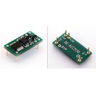
To elaborate on the above description on accelerometers,
there are three methods that most accelerometers use in order to measure
acceleration: piezo-electric, strain gauge, and capacitive.Piezo-electrical based accelerometers contain crystal structures that become stressed due to acceleration forces. Piezo based designs are unable to measure DC but are able to measure higher frequencies.
Strain gauge based acceleration detection uses adhesive backings that deform when forces are applied. This deformation alters the resistance of the object. That resistance can then be measured and the acceleration can be calculated. Strain gauge based designs are able to measure DC but are unable to measure at high frequencies.
Capacitance based designs utilize a mass attached to the plates of a capacitor. When the mass vibrates the capacitance is augmented. This change in capacitance can be measured and then the acceleration applied to the sensor can be calculated. A capacitance based design performs well in the same frequency ranges as a strain gauge but is generally more rugged.
The Buffered 3D 3g Accelerometer from Dimension Engineering is the most advanced analog accelerometer solution to date, featuring a triple axis ±3g accelerometer chip. It also has integrated op amp buffers for direct connection to a microcontroller's analog inputs, or for driving heavier loads.
Ultrasonic Range Sensors
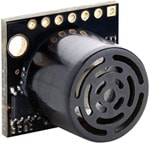
These range sensors test how close you are to an object by using sonar waves. These will bounce off an object and the time it took for the wave to get back to the sensor is used to calculate the distance from the object. These come in all distances and strengths but can be very accurate. Mounting these sensors on a servo can be a great way to get a wide range of readings without needing very many servos/range sensors. More details on Range sensors can be found on this items description page, HRLV-MaxSonar-EZ3 Ultrasonic Range Finder.

Depending on the application, a wide or narrow beam wave might be a better fit. The HRLV-MaxSonar-EZ0 has the widest and most sensitive beam pattern of any unit from HRLV-MaxSonar-EZ sensor line. This makes the HRLV-MaxSonar-EZ0 an excellent choice for use where high sensitivity, wide beam, or people detection is desired. The HRLV-MaxSonar-EZ4 is the narrowest beam width sensor that is also the least sensitive to side objects offered in the HRLV-MaxSonar-EZ sensor line. The HRLV-MaxSonar-EZ4 is an excellent choice when only larger objects need to be detected.
Wheel Encoders
Optical Encoders 
Optical encoders use a rotor disc made of plastic or glass
that is patterned with transparent and opaque areas that can be detected
as the disc rotates between a light source and a photodetector. Like
the magnetic encoder, the simplest configuration might use just one
sensor and have one half of the disc transparent and the other half
opaque. But for higher resolution, the disc is usually divided into many
more segments (often in concentric rings) with two or more sensors.
Magnetic Encoders 
Magnetic encoders use a combination of permanent magnets and
magnetic sensors to detect movement and position. A typical construction
uses magnets placed around the edge of a rotor disc attached to a shaft
and positioned so the sensor detects changes in the magnetic field as
the alternating poles of the magnet pass over it.Damage Prevention
Common sensors to prevent damage to the robot are related to object detection as discussed above. Other sensors such as current, temperature and humidity can also be employed to better protect the robot from itself as well as the environment. Knowing what's around your robot is normally the first step in damage prevention. The next step is to ensure that the characteristic of that environment, such as humidity and ambient gas, are not able to cause a catastrophic event.Once you have the appropriate sensor array to protect the robot from the environment you need to protect the robot from itself. Contact sensors and encoders are often used to set firm limits on robot movement. When a robot has attachments such as a pan-and-tilt camera or an arm there are typically ranges of movement that are save and ranges that would cause the robot to harm itself. Identifying these limits is key to developing a solid robotic solution. Once the movement limits have been addressed, it's important to monitor the current going to the motors as well as their temperature. Knowing the specifications of the motors and the motor controller will provide you with the safe limits of your drive system. Dynamically responding to these limits will help prevent motor stalling and overheating which can leave your robot stranded in a potentially dangerous environment and cause expensive permanent damage.
The crucial subject of timer and position sensor , so do for case discussion Tactical Robot
Industrial Force Tactical Robot subject to be we practical on Police, Fire, Rescue, Military, HAZMAT, Tactical Robots built specifically to provide video and audio surveillance for dangerous/hazardous situation keeping people out of harm's way.
Position Sensors
Position Sensors play an important role in our daily lives as they are abundant in domestic products, automobiles, and in office or industry places, etc. Position Sensors, as the name indicates, provide feedback on the position of the measurand (quantity being measured).Position sensors provide motion control, counting and encoding tasks by determining the presence or absence of a target or by detecting its direction, speed, motion or distance.
A position sensor can detect the position of an object or disturbance of electric or magnetic field and convert that physical parameter into an output electrical signal to indicate the position of the target.
As the technology improves, the sensing devices continue to get smaller, more inexpensive and better at performance, opening a gateway for more applications.
Types of Position Sensors
Position sensors are generally divided into two types based on the way of sensing.They are
- Contact Devices
- Non-contact Devices
Non-contact devices don’t involve in physical contact with the object. They are magnetic sensors, proximity sensors, Hall Effect based sensors and ultra-sonic sensors.
Every position sensor has its benefits and limitations. The goal is to select a sensor that is a cost effective solution for parameters of a specific application.
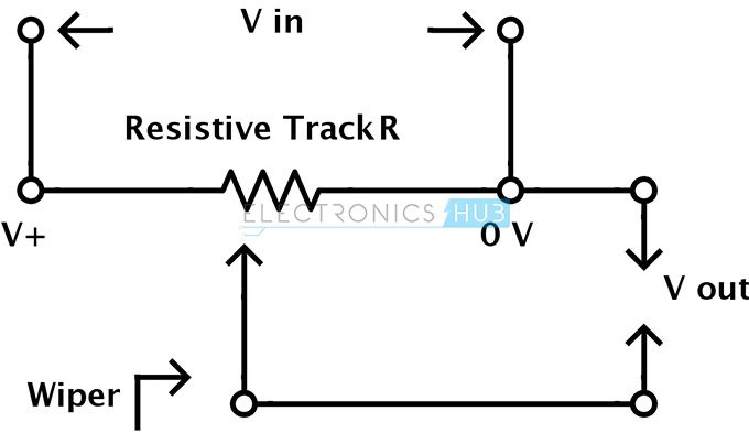
Resistance based or Potentiometric Position Sensor
Resistive position sensors are also called as Potentiometers or Position Transducers. They are originally developed for applications in military use. They were used in radios and televisions as panel mounted adjustment knobs. Potentiometers can work as linear or rotary position sensors.Potentiometer doesn’t require a power supply or extra circuitry to perform their basic position sensing function. Hence, they are passive devices. They are operated in two modes: voltage divider and rheostat. In rheostat, the resistance varies with motion. Hence the applications make use of this varying resistance between fixed terminal and a sliding contact. Voltage divider has the true potentiometric operation. In this, a reference voltage is applied across a resistive element. The position of the movable wiper is determined by calculating the voltage picked up by the wiper.
Potentiometers are the most commonly used position sensors. It has a fixed terminal and a wiper terminal connected to a mechanical shaft. The movement can be either linear (slide) or angular (rotational). This movement causes the resistance between fixed and wiper terminals to change. The output electrical signal which is generally voltage varies in proportion to the position of the wiper resistive track and hence the value of the resistance.
Potentiometers are available in different sizes and designs. The commonly available types are linear slider and rotational type. When it is used as position sensor, the object is connected to its slider.
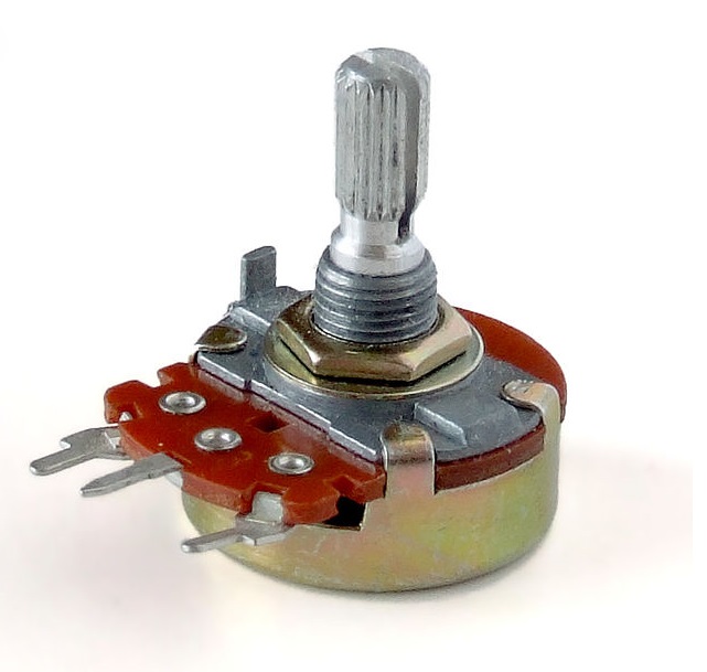
Image Resource Link: en.wikipedia.org/wiki/Potentiometer
A reference voltage is applied between
the fixed terminals which are on the either side of the wiper and the
output voltage is taken from this wiper. This configuration forms a
voltage divider network and the output voltage is dependent on the
position of the slider.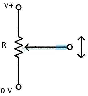
If a potential of 12 V is applied to the potentiometer, a maximum of 12 V and a minimum of 0 V is available as the output voltage. Depending on the position of the wiper, the output voltage can be any value between 0 V to 12 V. If the wiper is at the center of the resistive track, the output voltage is 6 V.
The construction of a potentiometer is shown in the below figure.
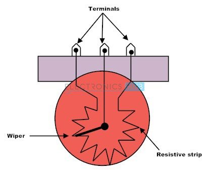
For general purpose position sensing, a low cost potentiometer is sufficient. The advantages of the potentiometers are low cost, simple operation, simple application theory, easy to use and robust EMI susceptibility. The disadvantages are eventual wear-out due to sliding wiper, lesser sensing angle and low accuracy. The main disadvantage of potentiometer based position sensor is its physical size as it limits the movement of the slide and hence the output signal. The sensing angle of a typical potentiometer is in the range of 00 to a maximum between 2400 and 3300. Vernier turns can be applied to achieve multi-turn capability.
A simple position sensing circuit is shown below.
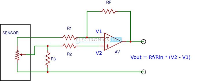
It consists of an OP amp and a potentiometer based position sensor. The output voltage depends on the position of the wiper.
Carbon film is the most common type of resistive track used in potentiometers. But there is a contact noise that is superimposed in the expected resistance. Contact noise is the result of mechanical contact between wiper and resistive surface. This can cause up to 5 % of the total resistance.
Wire wound type potentiometers use a straight wire resistive element or coil wound resistive wire. The problem with wire wound potentiometers is the jumping of wiper between positions producing a logarithmic output signal.
Polymer film or cermet type potentiometers are available for high precision and low noise applications. These are made up of conductive plastic resistive material. They have very less friction between the wiper and the surface and therefore less electrical noise, good resolution and longer life. These are available as both single turn and multi turn devices. These devices are used in high accuracy applications like joysticks, industrial robots etc.
Capacitive Position Sensors
Capacitive Sensors are non-contact type of devices used for precision measurement of a target position if the target is conductive in nature, or used for measurement of thickness and density of a material if the target is non-conductive in nature. When used with conductive targets, they work irrespective of the material of the target as all conductors look same to a capacitive sensor. The thickness of the target is also not important as the sensors sense the surface of the target. They are mainly used in disk drives, semiconductor technology and high precision manufacturing industries where high accuracy and frequency response are important. When used with non-conductive targets, they are generally used in label detectors, coating thickness monitors, and paper and film thickness measuring units.They are primarily used in measurement of linear displacement from a few millimeters to nanometers. Capacitive sensors make use of the electrical property conductance for measuring position. The ability to store electric charge by a body is capacitance. The most common device used to store charge is a parallel plate capacitor. The capacitance of a parallel plate capacitor is directly proportional to the surface area of the plates and dielectric constant, and inversely proportional to the distance between the plates. Hence, when the spacing between the plates is changed, there is a change in its capacitance and capacitive sensors make use of this property.
The capacitance,
C = (εr εo A) / d
Where
εr is relative permittivity of dielectric
εo is permittivity of free space
A is the overlap area of plates
And d is distance between the plates
A typical capacitive sensing model
consists of two metal plates with air in between them acting as
dielectric. The sensor or probe is one of the metal plates and the
target object which is conductive, is the other plate.When a potential is applied to the plates of the conductor, an electric field is created between them by causing positive charges to collect on one plate and negative charges on other.
Capacitive sensors use alternating voltage. Alternating voltage causes the charges to continually reverse their positions. The alternating electric field between the capacitive probe and the target is monitored for changes and is used in measuring the capacitance between the probe and target. Capacitance is determined by the area of the surfaces, dielectric constant and spacing of the surfaces. In the majority of capacitive sensing applications, the size and area of the capacitive sensor and the target do not change. The dielectric material between the conductive surfaces doesn’t change. The only factor responsible for any changes in the capacitance is the distance or spacing between the capacitive sensor and the target.
Hence the capacitance is an indicator of the target’s position. Capacitive sensors are calibrated to produce an output voltage corresponding to the change in distance between the probe and target which causes the capacitance to change. This is called the sensitivity of the capacitive sensor. Sensitivity of a capacitive sensor is the amount of voltage change to a defined amount of distance change. Generally used sensitivity setting is 1 V / 100 µ m i.e. the output voltage changes 1 V for every 100 µ m change in distance.
A capacitive sensor probe consists of three components: sensing area, guard and body.
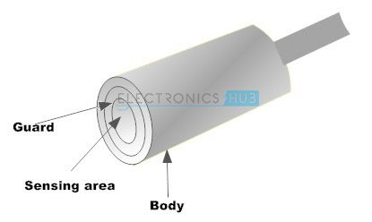
The potential is applied to the sensing area. There is a problem of spreading of an electric field to areas on the target other than the defined sensing area and the target. To prevent this from happening, a technique called guarding is used. In this technique, a guard area is created by surrounding the sides and back of the sensing area and is maintained at a potential same as the sensing area. As the guard and the sensing area are at the same potential, there will be no electric field between them. Any other conductors in the proximity other than the sensing area will form an electric field with the guard. The sensing area and the corresponding target are undisturbed.
Because of this guard, the electric field projection of the sensing area will be conical in nature. The electric field from the probe covers an area on the target of approximately 30 % larger that the sensor area. Therefore, it is essential to have a minimum target diameter as 30 % of the sensing areas’ diameter for standard calibration.
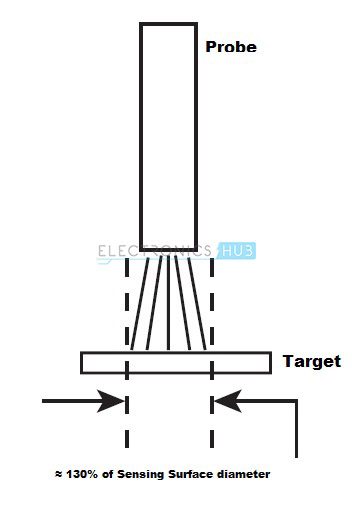 The
range of a sensing probe is directly proportional to the size of the
sensing area. Smaller probes must be placed closer to the target in
order to achieve the desired amount of capacitance. The maximum
allowable gap between the probe and the target is approximately 40% of
the diameter of the sensing area. Beyond this, the probe becomes
useless. There are applications where multiple probes are simultaneously
used. In these applications, it is essential to synchronize the
excitation voltage of all the probes. If the voltages are not
synchronized, the probes interfere with each other as one probe may try
to increase the electric field while the other decreases it. This gives a
false reading.
The
range of a sensing probe is directly proportional to the size of the
sensing area. Smaller probes must be placed closer to the target in
order to achieve the desired amount of capacitance. The maximum
allowable gap between the probe and the target is approximately 40% of
the diameter of the sensing area. Beyond this, the probe becomes
useless. There are applications where multiple probes are simultaneously
used. In these applications, it is essential to synchronize the
excitation voltage of all the probes. If the voltages are not
synchronized, the probes interfere with each other as one probe may try
to increase the electric field while the other decreases it. This gives a
false reading.Capacitive Sensors can also be used with non-conducting targets. The dielectric constant of the non-conductive target is the basis for the operation. The dielectric constant of the non-conductive materials like plastic is different than air. When the non-conducting material is used as a dielectric medium between two conducting plates, its dielectric constant will determine the capacitance between the conductors.
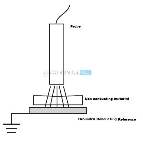 The
two conducting plates are sensor probe and a grounded conductive
reference. The changes in capacitance and hence the output of the sensor
will be corresponding to the changes in material thickness, density or
composition.
The
two conducting plates are sensor probe and a grounded conductive
reference. The changes in capacitance and hence the output of the sensor
will be corresponding to the changes in material thickness, density or
composition.There are high precision and high performance capacitive sensors that can measure a displacement of the order of nanometers. These high performance sensors are stable to changes in temperature, produce a linear output and have high resolution.
The advantages of capacitive sensors over other non-contact devices are high resolution, inexpensive and not sensitive to the material of the target. The capacitive sensors are not suitable in conditions where the environment is dry or wet and the distance between the probe and the target is large.
Inductive Position Sensors
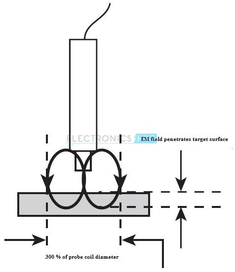
Inductive Sensors are non-contact type of devices used for precision measurement of a target position if the target is conductive in nature. Inductive sensors are used to recognize any conducting metal target.Capacitive sensors make use of electric field for sensing the surface of a conducting target. Inductive sensors make use of electromagnetic field that penetrates through the target. An inductive sensor probe consists of an oscillator that generates a high frequency electromagnetic field. This field is radiates from the sensing face of the probe.
Image Resource Link: baumer.com/typo3temp/pics/User_Knowledge_Presence_Inductive_Functionality_sensor_EN_216cc0d8dd.jpg
When this field contacts a conducting
metal target, a small current is induced within the metal target. These
currents will generate their own electromagnetic field that interferes
with the field originating from the probe. This causes a change in the
amplitude of the oscillations of the signals from the probe. The output
voltage can be calibrated to this change. When the probe is closer to
the target, the more current reacts with the field originating from the
probe and the output is greater.Unlike capacitive sensors, inductive sensors are independent of the material in the gap between the probe and the target. Hence, they can be used in hostile environment where oil or other liquids may appear in the gap.
The material of the target is an important factor in inductive sensors. Materials like aluminum, steel and copper, each react differently to the sensor. Hence the sensor must be calibrated for each target to achieve optimum to highest possible performance.
Generally there are two types of target materials for inductive sensors. They are ferrous and nonferrous. Ferrous materials are magnetic in nature while nonferrous materials are nonmagnetic. Ferrous materials include iron and most steel materials while nonferrous materials include zinc, aluminum, copper and brass. Some inductive sensors will work with both ferrous and nonferrous target materials while others will work only with one type of material.
The size of the target is also important as the effective area of electromagnetic field of the probe will vary from sensor to sensor. It is a minimum requirement to have the cross sectional area of the target of at least 300 % of the probe’s coil diameter, i.e. ideally the surface area of the target must be at least three times the diameter of the probe.
The thickness of the target is also an important factor as the electromagnetic field will penetrate the target and creates electrical currents. The thickness of the target depends on the frequency of the signal which drives the probe and is inversely proportional to the frequency, i.e. when the drive frequency increases, the minimum thickness of the target decreases.
For a drive frequency of 1 MHz, the minimum thickness of some commonly used target materials is as follows:
- Iron—0.6 mm
- Stainless Steel—0.4 mm
- Copper—0.2 mm
- Aluminum—0.25 mm
- Brass—1.6 mm
The output voltage and current of an inductive sensor is directly proportional to the distance between the surfaces of the sensor and the target, i.e. the voltage and current represent the absolute measured values corresponding to the distance. This property is used in numerous applications.
Linear Variable Differential Transformer (LVDT)
The Linear Variable Differential Transformer (LVDT) is a common type of electromechanical, high resolution, contact based linear position transducer. LVDT is one of the best available, reliable and accurate methods for measuring linear distance. LVDTs are used in computerized manufacturing, machine tools, avionics and robotics.Linear Variable Differential Transformer is a position to electrical sensor. An LVDT consists of three coils, one primary and two secondary. A movable magnetic core is placed as shown in the figure. This magnetic core which is also called an armature controls the transfer of current between primary and secondary coils in the LVDT. The output of the LVDT is proportional to the position of the core.
A cross sectional view of the LVDT is shown below.
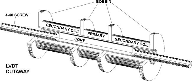
Image Resource Link: keckec.com/seismo/images/lvdtbig.gif
The magnetic core moves linearly inside
the transformer consisting of a primary coil and the two identical
outer secondary coils that are wound in a cylindrical manner.When the primary coil is excited with an alternating current, a voltage is induced across secondary coils. The secondary coil voltage varies according to the position of the magnetic core between the coils which moves axially. The output electrical signal is equal to the difference between the voltages across the secondary windings. Therefore the output voltage is proportional to the linear mechanical movement of the magnetic core.
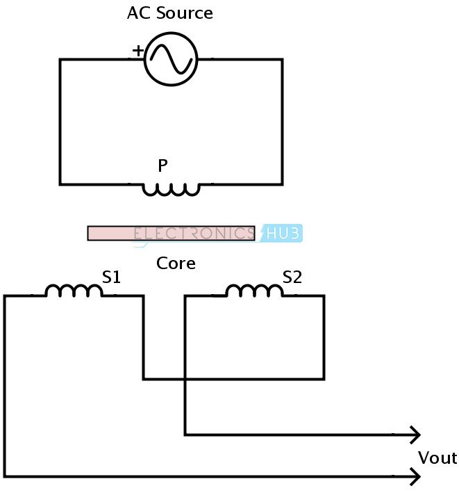
A normal transformer style representation of the LVDT is shown below.
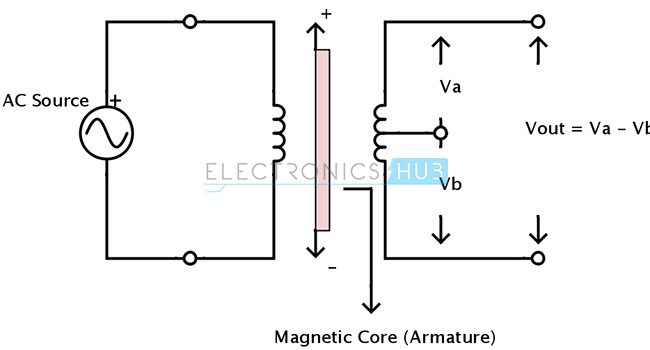
The schematic representation of an LVDT is as shown below.
Working of LVDT:
The primary coil of the transformer is energized by applying an alternating source of constant amplitude. This generates a magnetic field and the developed magnetic flux is coupled to the secondary coils S1 and S2 by the magnetic core in the center. The secondary coils are wound out of phase with each other. Therefore, when the position of the core is exactly midway between the two secondary coils, equal amount of magnetic flux is coupled to S1 and S2. The voltages induced in each of the secondary coils V1 and V2 are equal. Hence the output differential voltage Vout is equal to zero.
V1 = V2
And
Vout = V1 – V2 = 0
When the coil moves away from the
center, the voltage induced in each secondary coil is different. When
the core is moved towards S1, the magnetic flux coupled with S1 is
greater than that is coupled with S2. Therefore the induced voltage V1 increases and V2 decrease.
The differential output voltage is Vout = V1 – V2.
If the magnetic core or armature moves
towards the secondary coil S2, the magnetic flux coupled with S2 is
greater than S1. And the induced voltage V2 increases while V1 decreases. Therefore,
the output voltage is Vout = V2 – V1.
The phase of the output signal can determine the position of the core.Simply the output voltage of LVDT will not determine the position of the core if there are any mismatches between the secondary coils or any leakage inductances. A signal conditioning circuit is useful in removing these difficulties.
A normal LVDT is shown below.
LVDT with the signal conditioning circuit is shown below.
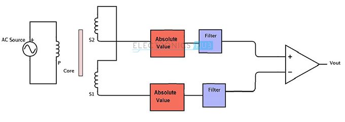
It consists of additional filtering and amplification circuit where the absolute values of the two output signals are subtracted. The absolute value circuit can be formed from a diode capacitor rectifier. Filters are used to detect the amplitude of both the secondary voltages. This technique is useful in measuring both the positive and negative variations about the center position.
LVDT has a huge advantage over the potentiometer as a position sensor in many ways. Since the magnetic core doesn’t touch the coils, there is no mechanical contact between the coils and the core. Hence a frictionless operation is achieved and is useful in testing and high resolution devices. This is also an important factor in their longer operation life.
Because of its electromagnetic coupling principles and frictionless operation, LVDT can measure infinitesimally small changes.
Inductive Proximity Sensors
Inductive Proximity Sensors are low cost, solid state and non-contact based devices. They are basically used to detect metal objects which are both ferrous and non-ferrous in nature. The basic components of an inductive proximity sensor are a coil, an oscillator, a detection circuit and an output circuit.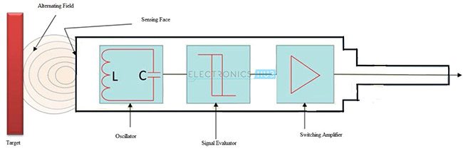
When an alternating current is passed through the coil, it generates a high frequency magnetic field. If a metallic object comes near to this field, the inductance of the coil changes. Eddy currents induced in the object by the field will change the amplitude of the oscillations. The demodulator will detect the changes in amplitude and converts them into a DC signal. This DC signal trips the trigger and the output stage switches.
Without any additional equipment, the inductive proximity sensor can operate electromagnetic clutches, brakes and valves. To actuate the sensor, a metal of any shape and size or a pneumatic cylinder or a machine tool carriage or a drill bit can be used.
The inductive proximity sensor ignores non-metallic objects like oil, water, dirt, etc. It withstands in shock environments and is short circuit resistant.
They are used in industry automation for counting the products, in security systems as metal detectors and in military applications in detecting landmines and other arms.
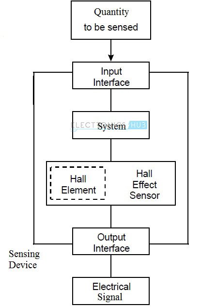
Hall Effect Based Magnetic Position Sensors
Magnetic Position Sensors are used to determine the position of objects by detecting the strength or direction or presence of magnetic fields generated from the Earth, electric currents, magnets and even brain wave activity. Magnetic position sensors are non-contact devices and are very important in many industries and navigation systems.The magnetic field is a vector quantity that has both magnitude as well as direction. Some sensors measure magnitude, but not direction of the magnetic field. These are scalar sensors. Other sensors measure the magnitude of the component of magnetization along their main sensitive axis. These are uni-directional sensors. Some sensors include direction of the field along with its magnitude. These are bi-directional sensors.
Hall Effect sensor is a magnetic field sensor and can be used in sensing position, pressure, current, temperature and many more.
A general Hall Effect sensor is shown below.
Position Sensors play an important role in our daily lives as they are abundant in domestic products, automobiles, and in office or industry places, etc. Position Sensors, as the name indicates, provide feedback on the position of the measurand (quantity being measured).
Position sensors provide motion control, counting and encoding tasks by determining the presence or absence of a target or by detecting its direction, speed, motion or distance.
A position sensor can detect the position of an object or disturbance of electric or magnetic field and convert that physical parameter into an output electrical signal to indicate the position of the target.
As the technology improves, the sensing devices continue to get smaller, more inexpensive and better at performance, opening a gateway for more applications.
Types of Position Sensors
Position sensors are generally divided into two types based on the way of sensing.They are
- Contact Devices
- Non-contact Devices
Non-contact devices don’t involve in physical contact with the object. They are magnetic sensors, proximity sensors, Hall Effect based sensors and ultra-sonic sensors.
Every position sensor has its benefits and limitations. The goal is to select a sensor that is a cost effective solution for parameters of a specific application.
Inductive Position Sensors Inductive Sensors are non-contact type of devices used for precision measurement of a target position if the target is conductive in nature. Inductive sensors are used to recognize any conducting metal target.
Capacitive sensors make use of electric field for sensing the surface of a conducting target. Inductive sensors make use of electromagnetic field that penetrates through the target. An inductive sensor probe consists of an oscillator that generates a high frequency electromagnetic field. This field is radiates from the sensing face of the probe.
Image Resource Link: baumer.com/typo3temp/pics/User_Knowledge_Presence_Inductive_Functionality_sensor_EN_216cc0d8dd.jpg
When this field contacts a conducting
metal target, a small current is induced within the metal target. These
currents will generate their own electromagnetic field that interferes
with the field originating from the probe. This causes a change in the
amplitude of the oscillations of the signals from the probe. The output
voltage can be calibrated to this change. When the probe is closer to
the target, the more current reacts with the field originating from the
probe and the output is greater.Unlike capacitive sensors, inductive sensors are independent of the material in the gap between the probe and the target. Hence, they can be used in hostile environment where oil or other liquids may appear in the gap.
The material of the target is an important factor in inductive sensors. Materials like aluminum, steel and copper, each react differently to the sensor. Hence the sensor must be calibrated for each target to achieve optimum to highest possible performance.
Generally there are two types of target materials for inductive sensors. They are ferrous and nonferrous. Ferrous materials are magnetic in nature while nonferrous materials are nonmagnetic. Ferrous materials include iron and most steel materials while nonferrous materials include zinc, aluminum, copper and brass. Some inductive sensors will work with both ferrous and nonferrous target materials while others will work only with one type of material.
The size of the target is also important as the effective area of electromagnetic field of the probe will vary from sensor to sensor. It is a minimum requirement to have the cross sectional area of the target of at least 300 % of the probe’s coil diameter, i.e. ideally the surface area of the target must be at least three times the diameter of the probe.
The thickness of the target is also an important factor as the electromagnetic field will penetrate the target and creates electrical currents. The thickness of the target depends on the frequency of the signal which drives the probe and is inversely proportional to the frequency, i.e. when the drive frequency increases, the minimum thickness of the target decreases.
For a drive frequency of 1 MHz, the minimum thickness of some commonly used target materials is as follows:
- Iron—0.6 mm
- Stainless Steel—0.4 mm
- Copper—0.2 mm
- Aluminum—0.25 mm
- Brass—1.6 mm
The output voltage and current of an inductive sensor is directly proportional to the distance between the surfaces of the sensor and the target, i.e. the voltage and current represent the absolute measured values corresponding to the distance. This property is used in numerous applications.
Linear Variable Differential Transformer (LVDT)
The Linear Variable Differential Transformer (LVDT) is a common type of electromechanical, high resolution, contact based linear position transducer. LVDT is one of the best available, reliable and accurate methods for measuring linear distance. LVDTs are used in computerized manufacturing, machine tools, avionics and robotics.Linear Variable Differential Transformer is a position to electrical sensor. An LVDT consists of three coils, one primary and two secondary. A movable magnetic core is placed as shown in the figure. This magnetic core which is also called an armature controls the transfer of current between primary and secondary coils in the LVDT. The output of the LVDT is proportional to the position of the core.
A cross sectional view of the LVDT is shown below.
Image Resource Link: keckec.com/seismo/images/lvdtbig.gif
The magnetic core moves linearly inside
the transformer consisting of a primary coil and the two identical
outer secondary coils that are wound in a cylindrical manner.When the primary coil is excited with an alternating current, a voltage is induced across secondary coils. The secondary coil voltage varies according to the position of the magnetic core between the coils which moves axially. The output electrical signal is equal to the difference between the voltages across the secondary windings. Therefore the output voltage is proportional to the linear mechanical movement of the magnetic core.
A normal transformer style representation of the LVDT is shown below.
The schematic representation of an LVDT is as shown below.
Inductive Proximity Sensors
Inductive Proximity Sensors are low cost, solid state and non-contact based devices. They are basically used to detect metal objects which are both ferrous and non-ferrous in nature. The basic components of an inductive proximity sensor are a coil, an oscillator, a detection circuit and an output circuit.When an alternating current is passed through the coil, it generates a high frequency magnetic field. If a metallic object comes near to this field, the inductance of the coil changes. Eddy currents induced in the object by the field will change the amplitude of the oscillations. The demodulator will detect the changes in amplitude and converts them into a DC signal. This DC signal trips the trigger and the output stage switches.
Without any additional equipment, the inductive proximity sensor can operate electromagnetic clutches, brakes and valves. To actuate the sensor, a metal of any shape and size or a pneumatic cylinder or a machine tool carriage or a drill bit can be used.
The inductive proximity sensor ignores non-metallic objects like oil, water, dirt, etc. It withstands in shock environments and is short circuit resistant.
They are used in industry automation for counting the products, in security systems as metal detectors and in military applications in detecting landmines and other arms.
Hall Effect Based Magnetic Position Sensors
Magnetic Position Sensors are used to determine the position of objects by detecting the strength or direction or presence of magnetic fields generated from the Earth, electric currents, magnets and even brain wave activity. Magnetic position sensors are non-contact devices and are very important in many industries and navigation systems.The magnetic field is a vector quantity that has both magnitude as well as direction. Some sensors measure magnitude, but not direction of the magnetic field. These are scalar sensors. Other sensors measure the magnitude of the component of magnetization along their main sensitive axis. These are uni-directional sensors. Some sensors include direction of the field along with its magnitude. These are bi-directional sensors.
Hall Effect sensor is a magnetic field sensor and can be used in sensing position, pressure, current, temperature and many more.
A general Hall Effect sensor is shown below.
Hall Effect devices when used as position sensors can be very accurate and affordable. Hall Effect sensor consists of a Hall element which is constructed from a thin sheet of conductive material. The output connections of the hall element are perpendicular to the direction of current flow. When a Hall Effect sensor is subjected to a magnetic field, it reacts with an output voltage that is proportional to the strength of the magnetic field. Additional electronic circuits like signal conditioning circuits are required to achieve useful voltage levels as the original output voltage is very small. Hence, a basic Hall Effect Sensor consists of a Hall element combined with a signal conditioning circuit on an integrated circuit.
The principle of Hall Effect states that, “when a current carrying conductor is placed in a magnetic field, a voltage is generated which is perpendicular to both current and magnetic field.”
Consider a thin sheet of conductive material. Current is passed through this and the output connection is perpendicular to the direction of the flow of current.
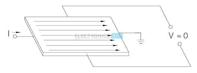
In the absence of a magnetic field, the current distribution is uniform and there is no potential difference in the output.
In the presence of a magnetic field perpendicular to the direction of the current, a Lorentz force is exerted on the current. This force disturbs the current distribution and results in a potential difference at the output.
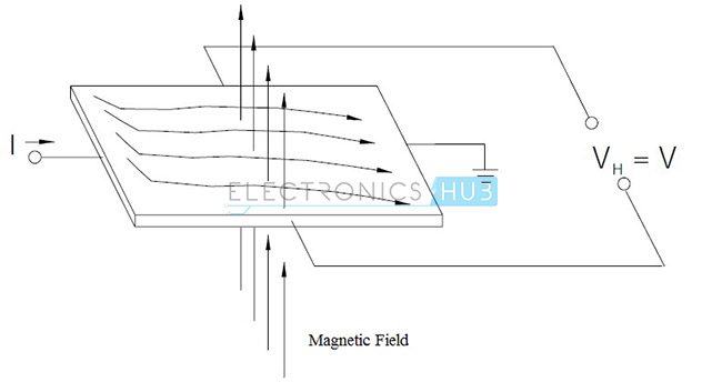
Hall Effect based position sensors are available with digital and analog output. In digital output sensors, the output is in either ON state or OFF state. Digital Hall Effect sensors are of two types: Bipolar and uni-polar. Bipolar sensors require positive gauss which is the South Pole to operate and negative gauss which is the North Pole to release. Release is obtained by moving the positive gauss or South Pole away from the sensor. Uni-polar sensors require a single magnetic pole to operate.
In analog output sensors, the output voltage is continuous and is dependent on the strength of the magnetic field. The output voltage increases or decreases with a strong or a weak magnetic field respectively. They operate by proximity to either of the magnetic poles.
Consider the following arrangement of a Hall Effect based position sensor.
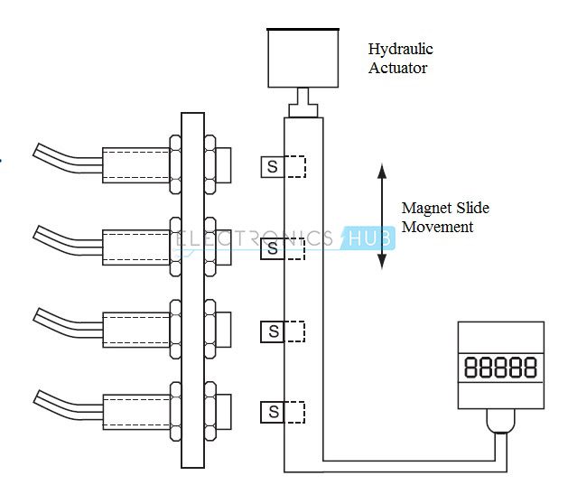
It consists of four uni-polar sensors with digital outputs and these four sensors are connected together and housed in an aluminum casing. These sensors are actuated by four individual magnetic actuators connected to a hydraulic system. The sensors generate event signals which represent the distance measured from a reference surface. These signals define the acceptable limits between which the object under test must generate electrical signals.
The following setup is used to achieve an accuracy of 0.002 inches of linear positioning. It consists of four bipolar sensors with digital outputs. They are actuated by a magnet mounted on a rod.
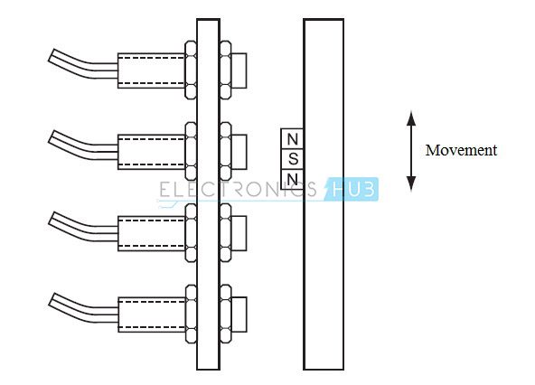
The advantages of Hall Effect sensors are long life, high speed and a temperature range of -40 0C to 150 0C.
Eddy Current Based Position Sensor
Eddy Current sensors are non-contact based devices used to measure the position, displacement, oscillation and vibration of a conductive target. Eddy current sensors are used in applications where high precision is required and the operating environment is harsh.Eddy current sensors work on the principle of magnetic induction. A simple Eddy current sensor consists of a driver and a sensing coil. When an alternating current is passed through the coil, it generates an alternating magnetic field. When a target comes in contact with this field, a small current is induced in the target. These currents are called Eddy Currents. The Eddy current in the target will create a field which opposes the field of the sensor and resist the field. The distance between the sensor and the target is the factor in interaction of the two magnetic fields. Hence, the output voltage is calibrated to the change in field interactions, which is dependent on the distance. The surface area of the target must be at least three times the diameter of the probe.
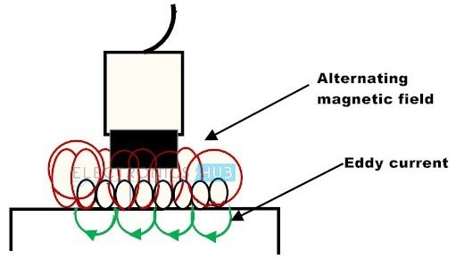
The advantages of Eddy Current Sensors are less expensive, tolerance to harsh and dirty environment, smaller in size and not sensitive to the type of material used in the gap between the sensor and target.
Eddy current sensors are less useful in applications where high resolution is required and the gap between the sensor and target is large.
Rotary Encoders
Rotary Encoder is an electromechanical device which converts angular motion to analog value or digital code. It is also called Shaft Encoder. Rotary encoders provide value as the shaft or axle of the encoder rotates. An output signal is produced that is proportional to the angle of the rotation. Based on the output signal, there are two types of encoders: incremental and absolute.The output of an Incremental Encoder is in the form of a square wave and provides information about the motion of the shaft. This information is processed into speed, position, distance and RPM.
The output of absolute encoders is in the form of absolute measure of position, i.e. they indicate the current position of the shaft. This makes them Angle Transducers. Both incremental and absolute encoders are available in two construction designs: optical and mechanical.
In applications where mechanical motion must be processed into digital information, the most popular choice of sensors is incremental encoders.
The structure of an incremental encoder is shown below.
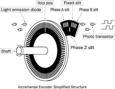
Image Resource Link: tamagawa-seiki.com/english/encoder/rotary01.jpg
Incremental encoders provide output of
pulse string that is proportional to the rotational displacement of the
shaft i.e. it provides output only when the shaft of the encoder is
rotated. To determine the amount of rotation, a counter is used that
counts the number of output pulses. From a certain input shaft position,
for the encoder to detect the amount of rotation, the count in the
counter is reset at a reference position and from that position the
number of pulses is added by the counter. The reference position can be
anywhere and the count can be unlimited.Incremental encoders are available in two channel types: single channel encoder and quadrature encoder. When the systems rotate in one direction, then single channel encoders are used. These are generally called Tachometers and provide only position and velocity information. Quadrature encoders have two output signals that are phased 900 apart. Hence quadrature encoders provide hi speed bi-directional information for complex motion applications.
Incremental optical encoders are used in applications where high RPM’s with high precision are calculated. Mechanical incremental encoders are generally used as digital potentiometers and require de-bouncing.
Absolute encoders produce a unique binary code output for each distinct angle of the shaft. The code can be gray code, excess gray code or natural binary code. The shaft position is always known in case of absolute encoders even after power failures.
The structure of an absolute encoder is shown below.
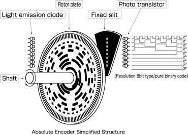
Image Resource Link: tamagawa-seiki.com/english/encoder/rotary02.jpg
Optical absolute encoders consist of a
glass or plastic disc with opaque and transparent areas. A light source
like an LED and an array photo detectors are used to read the optical
pattern resulting from the position of the disc at any time.Optical Position Sensors
Optical sensors convert light signals into electric signals. They are non-contact based sensors. It is similar to a photo resistor and measures the physical quantity and translates into a form that is readable by any appropriate instrument. Optical sensors can measure the following physical measurands: temperature, pressure, flow, liquid level, displacement, position, rotation, vibration, acceleration, force, velocity, strain, radiation, pH, magnetic field, electric field, acoustic field.Generally, the system employing optical sensor, includes three subsystems: a light source, a measuring device and an optical sensor. This is connected to an electrical trigger which reacts to changes in the signals in light sensor.
The example of an Optical Position Sensors is Position Sensitive Detector (PSD). Position sensitive detectors detect position data of incident light. Position sensitive detectors can track very small position changes. Position sensitive detectors can provide a high speed response, high reliability and high position resolution.
Fiber Optic Position Sensors
Fiber optic sensors use optical fibers as the sensing device. They can be used to sense temperature, strain, pressure, displacement, velocity and acceleration. The fiber optic position sensors make use of retro reflectance of light inside an optical fiber because of the movement of the proximal mirror surface. Fiber optic position sensors are immune to electromagnetic radiation, magnetic fields, lightning and many other harsh environmental conditions. They are generally used in long distance position sensing.A fiber optic position sensor consists of two parts: an optical technique embedded in a passive sensor and an active controller. These two are connected by a full duplex fiber optic link. The controller is used to send the light signals. It transmits a burst of light in the form similar to bar code to a code disc. The disc rotates and the code incident on the disc will be unique at every position. Only at a specific wavelength, the bar reflects the light and specific colors of light are returned to the controller over a separate fiber optic cable. The light is analyzed in the controller for wavelengths and an appropriate binary output is produced.
Fiber optic sensors are of two types: intrinsic and extrinsic sensors.
In intrinsic sensors, the measurand modulates the transmission properties of sensing optical fiber. The properties are intensity, polarization, phase, etc.
In extrinsic sensors, the modulation takes place outside the fiber. Here the optical fiber just acts as a conduit to transport light from and to the sensor head.
The advantages of fiber optic position sensors are:
- Immune to electromagnetic radiation.
- Consists of electrically insulating material.
- Wide temperature range.
- Ability to multiplex signals.