Develop Mathematical Model for Linear Program
with mathematical concepts to create all linear simulation models enable the forms, tools and models are
I D E A L P E R F E C T


X . I understanding mathematical model ideal (linear programming)
to make it easier to solve the problem of linear programming, namely Develop Mathematical Model for Linear Program. To make it easier to create a mathematical model, we have to read about the story carefully and understand the problem in depth. Here is the flow of real problems (in the form about the story) that is converted into a mathematical model (to be resolved) and then solved by linear programming. 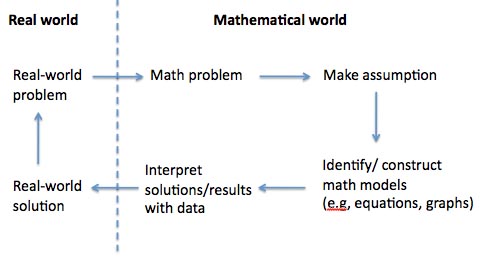


Understanding the Mathematical Model
The mathematical model is a simple way to translate a problem into mathematical language by using equations, inequalities, or function. Mathematical models of each problem in general linear program consists of two components, namely:
I. The objective function z = f (x, y) = ax + by
and
II. Functions of constraint (in the form of linear inequality system).
Steps to create mathematical models:
@. investigate a case study or problem carefully, and let (usually which is exemplified is the product).
@@. Arrange its inequality based constraints.
@@@. Arrange the objective function.
The characteristics of the inequality signs are used:
@). ≥ pins are used for the words: sodium absorption ratio is less than minimum, the smallest, at least, minimum, at least.
@). ≤ sign is used for words: more of the sodium absorption ratio, maximum, maximum, maximum, at the most.
Example question arrange Mathematical Model for Linear Program:
@). Sister will make two kinds of bread, which is bread and bread B. A Bread A requires 1 kg of wheat flour and 0.5 kg of eggs. While bread and requires 1.5 kg of flour and 1 kg of eggs. Sister only had 15 kg of wheat flour and 40 kg of eggs. If the number of buns A to be made is x and the amount of bread and to be made is y, then specify the model of math!
@). Sister will make two kinds of bread, which is bread and bread B. A Bread A requires 1 kg of wheat flour and 0.5 kg of eggs. While bread and requires 1.5 kg of flour and 1 kg of eggs. Sister only had 15 kg of wheat flour and 40 kg of eggs. If the number of buns A to be made is x and the amount of bread and to be made is y, then specify the model of math!
@). To make it easier to create mathematical models, these issues are presented in a table in advance.
@). Determine its shape inequality (constraint functions) based obstacles:
The first obstacle wheat flour:
The amount of flour needed to make both bread is (x + 1,5y) kg. Because inventory is 15 kg of wheat flour, the obtained relationship:
x + 1,5y≤15 or multiply 2: 2x + 3y≤30.
A second constraint eggs:
The number of eggs needed to make both bread is (0.5x + y) kg. Because the supply of eggs is 10 kg, the obtained relationship:
0.5x + y≤10 or multiply 2: x + 2y≤20
The third part:
x and y is the number of A bread and buns B so that x and y may not be negative. Therefore, x and y must satisfy the relationship:
x≥0 and y≥0, with x, y∈C.
Thus, the mathematical models is 2x + 3y≤30, x + 2y≤20, x≥0 and y≥0, with x, y∈C. C is a valid whole number consisting of {0,1,2,3,4,5, ...}.
@@ ). A tailor made two types of clothing, namely clothing children and adult clothing. One children's clothing takes 1 hour to phase cuts, 0.5 hours for obras stage, and 1.5 hours for the sewing stage. While one adult clothing takes 1.5 hours for the cutting stage, 1 hour to obras, and 2.5 hours for the sewing stage. The
tailors had time to work on orders for 20 hours for the cutting stage,
15 hours to stage obras, and 40 hours for the sewing stage. The net gain children's clothing and adult clothing is Rp15.000,00 and Rp30.000,00. Make a mathematical model of the linear programming problem in order to obtain the greatest possible advantage!
completion:@). Its products are children's clothing and adult clothing as well as the problem is the processing time is divided into three: cutting, pengobrasan, and suturing.Suppose the number of children's clothing = x and y = number of adult clothing. For convenience, the above issues are presented in tabular form as follows!
completion:@). Its products are children's clothing and adult clothing as well as the problem is the processing time is divided into three: cutting, pengobrasan, and suturing.Suppose the number of children's clothing = x and y = number of adult clothing. For convenience, the above issues are presented in tabular form as follows!
@). Develop constraint functions:cutting time: x + 2x + 1,5y≤20 or 3y≤40.obras time: 0.5x + y≤15 or x + 2y≤30.suturing time: + 2,5y≤40 1.5x or 3x + 5y≤80.Lots of positive things: x≥0, y≥0.@). Develop function or purpose or objective function objective function:z = 15.000x + 30.000y, or written f (x, y) = 15.000x + 30.000y.Wherein the objective function is a function of profit to be determined maximum value.
Thus, mathematical models are:Obstacles: 2x + 3y≤40, x + 2y≤30,3x + 5y≤80, x≥0, y≥0.The objective function: z = 15.000x + 30.000y.
III ). A practitioner requires two kinds of solutions, ie, a solution A and solution B for experiments. A solution containing 10 ml and 20 ml of material I II material. While the solution B containing 15 ml and 30 ml of material I II material. Solution A and solution B, will be used to prepare a solution C containing at least 40 ml of materials I and II ingredients at least 75 ml. Price per ml of solution A was Rp5.000,00 and each ml of solution B is Rp8.000,00. Make a model of math to keep the cost to prepare a solution C can be suppressed as small as possible!
completion:
@). Its products are the solution A and solution B and the problem is that the materials I and II.
Suppose the number of solution A is x and the amount of solution B is y.
@). Develop constraint functions based obstacles:
in the matter of using the word at least, means a sign of his skinfold equation "≥".
Materials I: 10x + 2x + 15y≥40 or 3y≥8.
Material II: 20x + 4x + 30y≥75 or 6y≥15.
Many positive solution: x≥0, y≥0.
@). Compiling the function purpose (as a function of cost):
z = 5.000x + 8.000y.
Thus, mathematical models are:
Obstacles: 2x + 3y≥8,4x + 6y≥15, x≥0, y≥0.
The objective function: z = 5.000x + 8.000y.
IIII). A trader sells two types of fruit, the watermelon and melon. The place is only able to accommodate as much as 60 kg of fruit. The merchant has the capital Rp140.000,00. The purchase price of watermelon Rp2.500,00 / kg and the purchase price of melon Rp2,000 / kg. Gains from the watermelon seller Rp 1,500.00 / kg and melons Rp1.250,00 / kg. Determine the mathematical model of this problem.
completion:
*). The product is the watermelon and melon, and the problem is the capacity of the basket and price.
Suppose watermelon and melon as much as x y.
Mathematical models table:

@). Develop appropriate constraint function limits:
Capacity: x + y≤60
Price: 2.500x + 2.000y≤140.000 or 5x + 4y≤280.
many positive fruits: x≥0, y≥0.
@). Develop objective function: z = 1.500x + 1.250y.
Thus, mathematical models are:
Barriers: x + y≤60,5x + 4y≤280, x≥0, y≥0.
The objective function: z = 1.500x + 1.250y.
IIIII). A parking lot has an area of 800 m2 and is only able to accommodate 64 buses and cars. A car spends a bus 6 m2 and 24 m2. Parking fee Rp1.500,00 / car and Rp2.500,00 / bus. Landowners parking expect maximum income. Determine the mathematical model of the problem.
completion:
@). Its products are cars and buses as well as capacity constraints (capacity) and land area.
Suppose cars and buses as much as x y.
Mathematical models table:

@). Develop constraint functions:
capacity: x + y≤64
Land area: 6x + 24y≤800.
Many positive vehicle: x≥0, y≥0.
@). Develop purpose function: z = 1.500x + 2.500y.
Thus, mathematical models are:
Obstacles: x + y≤64,6x + 24y≤800, x≥0, y≥0.
The objective function: z = 1.500x + 2.500y.
X . II Creating a Mathematical Model of Problems Related to Systems of Linear Equations Two Variables
@. In everyday life obtained a statement containing a system of linear equations of two variables that must be implemented ways we must first change the statements in question to form a system of equations linear.pernyataan-looking statements should be analyzed carefully and form a sentences mathematics or mathematical model in the form of a new system of equations we find the set penyelesaianya to the equation system of interpretation of the original question.Steps to create a system of linear equations of mathematical models of everyday problems:I. Identify the problem.II. Using the letters to change the prices of goods, many objects, or else.III. write the equationexample:Anselo buy rice 3kg and 2kg maize Rp 27.500,00. jessica buy 2kg 3kg of rice and corn in the same store at a price of Rp 29.000,00. go equation by replacing the variable price on rice and corn?replied:I. Identify the problem3 kg of rice and 2 kg of maize amount of Rp 27500.002 kg of rice and 3 kg of maize amount of Rp 29000.00II. replacing lettersExample:The price of rice = xThe price of corn = y
III. The system of equations obtained3x + 2y = USD 27500.002x + 3y = USD 29000.00
@@. Mathematical Model of Resolving Problems Related to Two-Variable Linear Equation System and Its interpretation.· Resolving issues related to systems of linear equations of two variables.Above have been taught how to make the system of equations of statements everyday to find the set of the completion of the mathematical model in the form of equations result of analysis problems can be solved by methods that have been taught.Steps to determine the set of equations completion of mathematical models everyday problems:
I) Identify the problem.II) Use letters to replace the item price, many objects, or otherIII) Writing equationIIII) Solve by finding the values of the lettersIIIII) Check the correctness of the calculation resultsExample:The difference of two numbers is 20 and twice the first number plus three times the second number is 100. determine the value of the two numbers that!Answer:I) Identification of the problemThe difference in the two numbers is 20The first two numbers plus plus three times the second number is 100.II) Using lettersFor example: the number I = a
numeral II = bIII) Writing equationA - b = 202a + 3b = 100IIII) Solving the equationa = 20 + b2 (20 + b) + 3b = 10040 + 2b + 3b = 1005b = 60
b = 12a = 20 + 12a = 32The set completion = {(32.12)}IIIII) Check the correctness of the calculation resultsa - b = 2032-12 = 20
20 = 20 (right)2a + 3b = 1002. (32) + 3 (12) = 100
64 + 36 = 100
100 = 100 (right)
X . III Mathematical Model (General)
If the physical phenomena created mathematical models is a continuous phenomenon (so it contains infinite elements, for example the phenomenon of light is a form of power with the smallest units called photons), the resulting mathematical model is a model approach.
A mathematical model as an approach to a phenomenon (natural or artificial) only covers as much to observation or cover only a limited area of the phenomenon (which is not limited) or only discrete, although the model is still considered a form which is ideal and a very approaching the original physical phenomena.
In the past, the branches of mathematics that study the continuous physical phenomena (waves, heat, elasticity of a material, fluid motion, etc.) dominate the branches of mathematics that can be applied to a variety of physical phenomena as commonly studied in physics and chemistry. As a result, the branches of mathematics is classified in the group of applied mathematics or mathematical physics.
But since the development of computer science, the application of the branches of mathematics who study the phenomena is not just a discrete, finite even, is expanding rapidly. For example, the concept of the field until the (English: finite fields) once considered as a pure branch of algebra is one of the important backbone in coding theory.
Similarly, the theory of measure (English: measure theory) more practice, particularly in relation to the theory of fractals and chaos theory. Of course mathematicians still studying aspects of the theory of fractals and chaos theory knowledge without having sizes.
For the finite physical phenomena, mathematical models (eg models and mathematical formulation for the signal, decoder and encoder code Reed-Muller), who made no longer a model approach, but it is the exact models.
In some specific branches of mathematics, the term 'mathematical model' can be narrowed and as a result, the definition or understanding (special) of the word 'mathematical model' in a branch of mathematics can be different from the meaning of the same word in another branch of mathematics.
Below is given a general overview of the group of mathematical models in a branch of mathematics that is large and spacious, although generally still classified in the group of applied mathematics.
X . IIII In Mathematical Model Optimization and Control
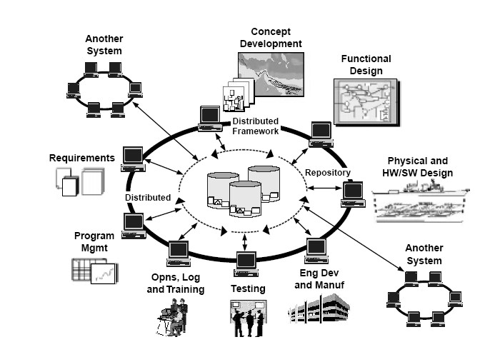
Often the engineer or engineer menganilisis a system of a phenomenon (natural or artificial) with the aim that the system can be controlled or optimized performance by creating mathematical models.
In the analysis, the engineer and the engineer can model a description of the system as an estimate (hypothesis) of how the system could work, or how future events might affect the system. Similarly, in pengkontrolan against a system, the engineers and engineers can try several ways to control through simulation.
A mathematical model in the optimization and control usually describes a system as a combination of a set of variables (variables) and a set of equations that express the relationship between these variables. The values of variables can be anything; in the form of natural numbers (real) or round, Boolean, or in the form of a row of figures and characters (strings).
The variables present some properties of the system, for example, the value of output (output) of the measurement results, timing data, calculators, many an event arise or recur, etc. Real mathematical models here are a set of functions that the relationship between the different variables.
For a more detailed reference (on the building blocks, objectives and constraints, the types of variables, etc., from this model, are welcome to read on
Model theory
In mathematics, model theory is the science that presents mathematical concepts through the concept of sets, or knowledge about models that support a mathematical system.
Model theory begins with the assumption of the existence of mathematical objects (eg, where all numbers) and then search and analyze the existence of operations, relationships or axioms that are attached to each object or collection of these objects.
The independence of the two mathematical laws - which is better known as the axiom of choice and the continuum hypothesis - from the axioms of set theory (proved by Paul Cohen and Kurt Gödel) are the two famous results obtained from Theory Model.
It has been proven that the axiom of choice and its negation are consistent with the axioms of Zermelo-Fraenkel set theory and the same result was also met by the continuum hypothesis. In an example of the application of methods Theory Model on axioms of set theory.
An example of a theoretical model to be presented by the set of all natural numbers R together himpunsn all relations and / or functions, such as {×, +, -,., 0, 1}.
Statement symbolized by
"∃y (y × y = 1 + 1)"
is true for y € R, because we can get to the root 2 as a solution. But the same statement is false when y is required to rational numbers.
The statement is somewhat similar
"∃y (y × y = 0-1)",
an incorrect value when y is required is real, but the statement is true if y is allowed complex-valued.
So the value of true or false a statement in a conversation about any element y of a set, depending on the set that contains the y. This set is called the set of the universe or the universe of discourse of the statement.
X . IIIII Model Theory
In mathematics, a model theory is the study of classes of mathematical structures (e.g. groups, fields, graphs, universes of set theory) from the perspective of mathematical logic. The objects of study are models of theories in a formal language. A set of sentences in a formal language is called a theory; a models of a theory is a structure (e.g. an interpretation) that satisfies the sentences of that theory.
Model theory Intimately recognises and is concerned with a duality: It examines semantical elements (meaning and truth) by means of syntactical elements (formulas and proofs) of a corresponding language. To quote the first page of Chang & Keisler (1990): [1]
universal algebra = + logic theory models.
Rapidly theory models developed during the 1990s, and a more modern definition is provided by Wilfrid Hodges (1997):
the model theory = algebraic geometry - fields,
Although models Also theorists are interested in the study of fields. Other nearby areas of mathematics include combinatorics, number theory, arithmetic dynamics, analytic functions, and non-standard analysis.
Similar in a way to proof theory, a model theory is situated in an area of interdisciplinarity Among mathematics, philosophy, and computer science. The most prominent professional organization in the field of the model theory is the Association for Symbolic Logic.
Branches of the model theory
This article focuses on finitary first-order model of theory of infinite structures. Finite models theory, the which concentrates on finite structures, Significantly diverges from the study of infinite structures in both the problems studied and the techniques used. Model theory in higher-order logics or infinitary logics is hampered by the fact that completeness and compactness do not in general hold for these logics. However, a great deal of study HAS ALSO been done in such logics.
Informally, the model theory can be divided into classical theory models, the model theory applied to groups and fields, and the geometric model of theory. A missing subdivision is Computable model of theory, but this can arguably be Viewed as an independent subfield of logic.
Examples of early theorems from classical theory models include Gödel's completeness theorem, the upward and downward Löwenheim-Skolem theorems, Vaught's two-cardinal theorem, Scott's isomorphism theorem, the omitting types theorem, and the Ryll-Nardzewski theorem. Examples of early results from the model theory applied to fields are Tarski's elimination of quantifiers for real closed fields, Ax's theorem on pseudo-finite fields, and Robinson's development of non-standard analysis. An important step in the evolution of classical theory models occurred with the birth of stability theory (through Morley's theorem on uncountably categorical theories and Shelah's classification program), the which developed a calculus of independence and rank based on syntactical conditions satisfied by theories.
During the last Several Decades repeatedly applied the model theory has merged with the more pure stability theory. The result of this synthesis is called the geometric model of theory in this article (which is taken to include o-minimality, for example, as well as classical geometric stability theory). An example of a theorem from geometric models Hrushovski's theory is proof of the Mordell-Lang conjecture for function fields. The ambition of the geometric model of theory is to provide a geography of mathematics by embarking on a detailed study of definable sets in various mathematical structures, aided by the substantial tools developed in the study of pure theory models.
Universal algebra
Fundamental concepts in universal algebra are signatures σ and σ-algebras. Since these concepts are formally defined in the article on structures, the present article is an informal introduction which consists of examples of the way these terms are used.- The standard signature of rings is σring = {×,+,−,0,1}, where × and + are binary, − is unary, and 0 and 1 are nullary.
- The standard signature of semirings is σsmr = {×,+,0,1}, where the arities are as above.
- The standard signature of groups (with multiplicative notation) is σgrp = {×,−1,1}, where × is binary, −1 is unary and 1 is nullary.
- The standard signature of monoids is σmnd = {×,1}.
- A ring is a σring-structure which satisfies the identities u + (v + w) = (u + v) + w, u + v = v + u, u + 0 = u, u + (−u) = 0, u × (v × w) = (u × v) × w, u × 1 = u, 1 × u = u, u × (v + w) = (u × v) + (u × w) and (v + w) × u = (v × u) + (w × u).
- A group is a σgrp-structure which satisfies the identities u × (v × w) = (u × v) × w, u × 1 = u, 1 × u = u, u × u−1 = 1 and u−1 × u = 1.
- A monoid is a σmnd-structure which satisfies the identities u × (v × w) = (u × v) × w, u × 1 = u and 1 × u = u.
- A semigroup is a {×}-structure which satisfies the identity u × (v × w) = (u × v) × w.
- A magma is just a {×}-structure.
Terms such as the σring-term t(u,v,w) given by (u + (v × w)) + (−1) are used to define identities t = t', but also to construct free algebras. An equational class is a class of structures which, like the examples above and many others, is defined as the class of all σ-structures which satisfy a certain set of identities. Birkhoff's theorem states:
- A class of σ-structures is an equational class if and only if it is not empty and closed under subalgebras, homomorphic images, and direct products.
 , where I is an infinite set indexing a system of σ-structures Ai, and U is an ultrafilter on I.
While model theory is generally considered a part of mathematical logic, universal algebra, which grew out of Alfred North Whitehead's (1898) work on abstract algebra, is part of algebra. This is reflected by their respective MSC classifications. Nevertheless, model theory can be seen as an extension of universal algebra.
Finite models theory
Finite model of theory is the area of the model theory, the which has the closest ties to universal algebra. Like some parts of universal algebra, and in contrast with the other areas of the model theory, it is mainly concerned with finite algebras, or more Generally, with finite σ-structures for signatures σ roomates may contain relation symbols as in the following example:
The standard signature for graphs is σgrph = {E}, where E is a binary relation symbol.
A graph is a σgrph-structure satisfying the sentences ∀ u ∀ v (u E v → v E u) {\ displaystyle \ forall u \ forall v (uEv \ RightArrow Veu)} \ forall u \ forall v (uEv \ RightArrow Veu ) and ∀ u ¬ (u E u) {\ displaystyle \ forall u \ neg (uEu)} \ forall u \ neg (uEu).
A σ-homomorphism is a map that commutes with the operations and preserves the relations in σ. This definition Gives rise to the usual notion of graph homomorphism, the which has the interesting property that a bijective homomorphism need not be invertible. Structures are Also a part of universal algebra; after all, some algebraic structures such as ordered groups have a binary relation <. What distinguishes finite models from universal algebra theory is its use of more general logical sentences (as in the example above) in place of identities. (In a Model-theoretic context an identity t = t 'is written as a sentence ∀ u 1 u 2 ... un (t = t') {\ displaystyle \ forall u_ {1} u_ {2} \ dots u_ {n} (t = t ')} \ forall u_ u_ {1} {2} \ dots u_ {n} (t = t').)
The logics employed in finite models Often theory are substantially more expressive than first-order logic, the standard logic for the model theory of infinite structures.
First-order logic
Whereas universal algebra Provides the semantics for a signature, logic Provides the syntax. With terms, identities and quasi-identities, even universal algebra has some limited syntactic tools; first-order logic is the result of making Quantification explicit and adding negation into the picture.
A first-order formula is built out of atomic formulas such as R (f (x, y), z) or y = x + 1 by means of the Boolean connectives ¬, ∧, ∨, → {\ displaystyle \ neg, \ land, \ lor, \ RightArrow} \ neg, \ land, \ lor, \ RightArrow and prefixing of quantifiers ∀ v {\ displaystyle \ forall v} \ forall v or ∃ v {\ displaystyle \ exists v} \ exists v. A sentence is a formula in the which each occurrence of a variable is in the scope of a corresponding quantifier. Examples for formulas are φ (or φ (x) to mark the fact that at most x is an unbound variable in φ) and ψ defined as follows:
φ = ∀ u ∀ v (∃ w (x × w = u × v) → (∃ w (x × w = u) ∨ ∃ w (x × w = v))) ∧ x ≠ 0 ∧ x ≠ 1, {\ displaystyle {\ varphi \; = \; \ forall u \ forall v (\ exists w (x \ times w = u \ times v) \ RightArrow (\ exists w (x \ times w = u) \ lor \ exists w (x \ times w = v))) \ land x \ neq 0 \ land x \ neq 1}} {\ varphi \; = \; \ forall u \ forall v (\ exists w (x \ times w = u \ times v) \ RightArrow (\ exists w (x \ times w = u) \ lor \ exists w (x \ times w = v))) \ land x \ neq 0 \ land x \ neq 1}
ψ = ∀ ∀ u v ((u × v = x) → (u = x) ∨ (y = x)) ∧ x ≠ 0 ∧ x ≠ 1. {\ displaystyle \ psi \; = \; \ forall u \ forall v ((u \ times v = x) \ RightArrow (u = x) \ lor (v = x)) \ land x \ neq 0 \ land x \ neq 1.} \ psi \; = \; \ forall u \ forall v ((u \ times v = x) \ RightArrow (u = x) \ lor (v = x)) \ land x \ neq 0 \ land x \ neq 1.
(Note that the equality symbol has a double meaning here.) It is intuitively clear how to translate such formulas into mathematical meaning. In the σsmr-structure N {\ displaystyle {\ mathcal {N}}} {\ mathcal {N}} of the natural numbers, for example, an element n satisfies the formula φ if and only if n is a prime number. The formula ψ similarly defines irreducibility. Tarski Gave a rigorous definition, sometimes called "Tarski's definition of truth", for the satisfaction relation ⊨ {\ displaystyle \ models} \ models, so that one Easily Proves:
N ⊨ φ (n) ⟺ n {\ displaystyle {\ mathcal {N}} \ models \ varphi (n) \ iff n} {\ mathcal {N}} \ models \ varphi (n) \ iff n is a prime number ,
N ⊨ ψ (n) ⟺ n {\ displaystyle {\ mathcal {N}} \ models \ psi (n) \ iff n} {\ mathcal {N}} \ models \ psi (n) \ iff n is irreducible.
A set T of sentences is called a (first-order) theory. A theory is satisfiable if it has a model of the M ⊨ T {\ displaystyle {\ mathcal {M}} \ models T} {\ mathcal {M}} \ models T, i.e. a structure (of the Appropriate signature) the which satisfies all the sentences in the set T. Consistency of a theory is usually defined in a syntactical way, but in first-order logic by the completeness theorem there is no need to extinguishing between satisfiability and consistency , Therefore, the model Often theorists use "consistent" as a synonym for "satisfiable".
A theory is called categorical if it determines a structure up to isomorphism, but it turns out that this definition is not useful, due to serious restrictions in the expressivity of first-order logic. The Löwenheim-Skolem theorem implies that for every theory T [2] the which has an infinite models then for every infinite cardinal number κ, there is a model of M ⊨ T {\ displaystyle {\ mathcal {M}} \ models T} {\ mathcal {M}} \ models T such that the number of elements of M {\ displaystyle {\ mathcal {M}}} {\ mathcal {M}} is exactly κ. Therefore, only finitary structures can be Described by a categorical theory.
Lack of expressivity (when Compared to higher logics such as second-order logic) has its advantages, though. For the model theorists, the Löwenheim-Skolem theorem is an important practical tool rather than the source of Skolem's paradox. In A Certain sense made precise by Lindström's theorem, first-order logic is the most expressive logic for the which both the Löwenheim-Skolem theorem and the compactness theorem hold.
As a corollary (i.e., its contrapositive), the compactness theorem says that every unsatisfiable first-order theory has a finite unsatisfiable subset. This theorem is of central importance in the model infinite theory, where the words "by compactness" are commonplace. One way to PROVE it is by means of Ultraproducts. An alternative proof uses the completeness theorem, the which is otherwise reduced to a marginal role in most of the modern theory models.
Axiomatizability, elimination of quantifiers, and the model-completeness
The first step, Often trivial, for applying the methods of the model theory to a class of mathematical objects such as groups, or trees in the sense of graph theory, is to choose a signature σ and represent the objects as σ-structures. The next step is to show that the class is an elementary class, i.e. axiomatizable in first-order logic (i.e. there is a theory T such that a σ-structure is in the class if and only if it satisfies T). E.g. this step fails for the trees, since connectedness can not be Expressed in first-order logic. Axiomatizability ensures that the model theory can speak about the right objects. Quantifier elimination can be seen as a condition the which ensures that the model theory does not say too much about the objects.
A theory T has quantifier elimination if every first-order formula φ (x1, ..., xn) over its signature is equivalent modulo T to a first-order formula ψ (x1, ..., xn) without quantifiers, i.e. ∀ x 1 ... ∀ xn (φ (x 1, ..., xn) ↔ ψ (x 1, ..., xn)) {\ displaystyle \ forall x_ {1} \ dots \ forall x_ {n} (\ phi (x_ { 1}, \ dots, x_ {n}) \ leftrightarrow \ psi (x_ {1}, \ dots, x_ {n}))} \ forall x_ {1} \ dots \ forall x_ {n} (\ phi (x_ {1}, \ dots, x_ {n}) \ leftrightarrow \ psi (x_ {1}, \ dots, x_ {n})) holds in all models of T. For example, the theory of algebraically closed fields in the signature σring = (x, +, -, 0.1) has quantifier elimination Because every formula is equivalent to a Boolean combination of equations between polynomials.
A substructure of a σ-structure is a subset of its domain, closed under all functions in its signature σ, the which is regarded as a σ-structure by restricting all functions and relations in σ to the subset. An embedding of a σ-structure A {\ displaystyle {\ mathcal {A}}} {\ mathcal {A}} into another σ-structure B {\ displaystyle {\ mathcal {B}}} {\ mathcal {B}} is a map f: A → B between the domains of the which can be written as an isomorphism of A {\ displaystyle {\ mathcal {A}}} {\ mathcal {A}} with a substructure of B {\ displaystyle {\ mathcal { B}}} {\ mathcal {B}}. Every embedding is an injective homomorphism, but the converse holds only if the signature contains no relation symbols.
If a theory does not have quantifier elimination, one can add additional symbols to its signature so that it does. Early models of theory spent much effort on proving axiomatizability and quantifier elimination results for specific theories, especially in algebra. But instead of quantifier elimination Often a Weaker property suffices:
A theory T is called the model-complete if every substructure of a T models of the which is itself a model of of T is an elementary substructure. There is a useful criterion for testing Whether a substructure is an elementary substructure, called the Tarski-Vaught test. It follows from this criterion that a theory T is a model-complete if and only if every first-order formula φ (x1, ..., xn) over its signature is equivalent modulo T to an existential first-order formula, i.e. a formula of the following form:
∃ v 1 ... ∃ vm ψ (x 1, ..., xn, v 1, ..., vm) {\ displaystyle \ exists v_ {1} \ dots \ exists v_ {m} \ psi (x_ {1}, \ dots, x_ {n} v_ {1}, \ dots, v_ {m})} \ exists v_ {1} \ dots \ exists v_ {m} \ psi (x_ {1}, \ dots, x_ {n}, v_ {1}, \ dots, v_ {m}),
where ψ is quantifier free. A theory that is not a model-complete may or may not have a model of completion, the which is a related-complete model of theory that is not, in general, an extension of the original theory. A more general notion is that of a model companions.
Categoricity
As observed in the section on first-order logic, first-order theories can not be categorical, i.e. they can not describe a unique model of up to isomorphism, UNLESS that the model is finite. But two-theoretic models of famous theorems deal with the Weaker notion of κ-categoricity for a cardinal κ. A theory T is called κ-categorical if any two models of T that are of cardinality κ are isomorphic. It turns out that the question of κ-categoricity depends critically on Whether κ is bigger than the cardinality of the language (ie ℵ 0 {\ displaystyle \ aleph _ {0}} \ aleph _ {0} + | σ |, where | σ | is the cardinality of the signature). For finite or countable signatures this means that there is a fundamental difference between ℵ 0 {\ displaystyle \ aleph _ {0}} \ aleph _ {0} -cardinality and κ-cardinality for uncountable κ.
A few characterizations of ℵ 0 {\ displaystyle \ aleph _ {0}} \ aleph _ {0} -categoricity include:
For a complete first-order theory T in a finite or countable signature the following conditions are equivalent:
T is ℵ 0 {\ displaystyle \ aleph _ {0}} \ aleph _ {0} -categorical.
For every natural number n, the Stone space Sn (T) is finite.
For every natural number n, the number of formulas φ (x1, ..., xn) in n free variables, up to equivalence modulo T, is finite.
This result, due Independently to Engeler, Ryll-Nardzewski and Svenonius, is sometimes Referred to as the Ryll-Nardzewski theorem.
Further, ℵ 0 {\ displaystyle \ aleph _ {0}} \ aleph _ {0} -categorical theories and their countable models have strong ties with oligomorphic groups. They are Often constructed as Fraisse limits.
Michael Morley's highly non-trivial result that (for countable languages) there is only one notion of uncountable categoricity was the starting point for the modern model of theory, and in particular classification theory and stability theory:
Morley's theorem categoricity
If a first-order theory T in a finite or countable signature is κ-categorical for some uncountable cardinal κ, then T is κ-categorical for all uncountable cardinals κ.
Uncountably categorical (i.e. κ-categorical for all uncountable cardinals κ) theories are from many points of view the most well-behaved theories. A theory that is both ℵ 0 {\ displaystyle \ aleph _ {0}} \ aleph _ {0} -categorical and uncountably categorical is called totally categorical.
Model theory and set theory
Set theory (which is Expressed in a countable language), if it is consistent, has a countable models; this is known as Skolem's paradox, since there are sentences in set theory, the which postulate the existence of uncountable sets and yet Reviews These sentences are true in our countable models. Particularly the proof of the independence of the continuum hypothesis requires considering sets in models roomates Appear to be uncountable when viewed from within the models, but are countable to someone outside the models.
The Model-theoretic viewpoint has been useful in set theory; for example in Kurt Gödel's work on the constructible universe, which, along with the method of forcing developed by Paul Cohen can be shown to PROVE the (again philosophically interesting) independence of the axiom of choice and the continuum hypothesis from the other axioms of set theory.
In the other direction, the model theory itself can be formalized within ZFC set theory. The development of the fundamentals of the model theory (such as the compactness theorem) Rely on the axiom of choice, or more exactly the Boolean prime ideal theorem. Other results in the model theory depend on set-theoretic axioms ZFC beyond the standard framework. For example, if the Continuum Hypothesis holds then every countable models has an ultrapower the which is saturated (in its own cardinality). Similarly, if the Generalized Continuum Hypothesis holds then every models has a saturated elementary extension. Neither of Reviews These results are provable in ZFC alone. Finally, some questions Arising from the model theory (such as compactness for infinitary logics) have been shown to be equivalent to large cardinal axioms.
Other Basic Notions of a model theoryReducts and expansions
A field or a vector space can be regarded as a (commutative) group by simply ignoring some of its structure. The corresponding notion in theory the model is that of a reduct of a structure to a subset of the original signature. The opposite relation is called an expansion - e.g. the (additive) group of the rational numbers, regarded as a structure in the signature {+, 0} can be expanded to a field with the signature {×, +, 1.0} or to an ordered group with the signature {+ , 0, <}.
Similarly, if σ 'is a signature that extends another signature σ, then a complete σ'-theory can be restricted to σ by intersecting the set of its sentences with the set of σ-formulas. Conversely, a complete σ-theory can be regarded as a σ'-theory, and one can extend it (in more than one way) to a complete σ'-theory. The reduct and expansion terms are sometimes applied to this relation as well.interpretability
Interpretation (model theory)
Given a mathematical structure, there are very often associated roomates structures can be constructed as a quotient of part of the original structure via an equivalence relation. An important example is a quotient group of a group.
One might say that to understand the full structure one must understand Reviews These quotients. When the equivalence relation is definable, we can give the previous sentence a precise meaning. We say that Reviews These structures are interpretable.
A key fact is that one can translate sentences from the language of the interpreted structures to the language of the original structure. Thus Spake one can show that if a structure M interprets another Whose theory is undecidable, then M itself is undecidable.
Using the compactness and completeness theorems
Gödel's completeness theorem (not to be confused with his Incompleteness Theorems) says that a theory has a model of if and only if it is consistent, i.e. no contradiction is proved by the theory. This is the heart of the model theory as it lets us answer questions about theories by looking at models and vice versa. One should not confuse the completeness theorem with the notion of a complete theory. A complete theory is a theory that contains every sentence or its negation. Importantly, one can find a complete consistent theory extending any consistent theory. However, as shown by Gödel's Incompleteness Theorems are relatively simple only in cases will it be possible to have a complete consistent theory that IS ALSO recursive, i.e. that can be Described by a recursively enumerable set of axioms. In particular, the theory of natural numbers has no recursive complete and consistent theory. Non-recursive theories are of little practical use, since it is undecidable if a proposed axiom is indeed an axiom, making proof-checking a supertask.
The compactness theorem states that a set of sentences S is satisfiable if every finite subset of S is satisfiable. In the context of proof theory the analogous statement is trivial, since every proof can have only a finite number of antecedents used in the proof. In the context of the model theory, however, this proof is somewhat more difficult,. There are two well known proofs, one by Gödel (which goes via proofs) and one by Malcev (which is more direct and Allows us to restrict the cardinality of the the resulting model).
Model theory is usually concerned with first-order logic, and many important results (such as the completeness and compactness theorems) fail in second-order logic or other alternatives. In first-order logic all infinite cardinals look the same to a language the which is countable. This is Expressed in the Löwenheim-Skolem theorems, the which state that any countable theory with an infinite model of A {\ displaystyle {\ mathfrak {A}}} {\ mathfrak {A}} has models of all infinite cardinalities (at least that of the language) roomates agree with A {\ displaystyle {\ mathfrak {A}}} {\ mathfrak {A}} on all sentences, ie they are 'elementarily equivalent'.
types
Fix an L {\ displaystyle L} L-structure M {\ displaystyle M} M, and a natural number n {\ displaystyle n} n. The set of definable subsets of M n {\ displaystyle M ^ {n}} M ^ {n} over some parameters A {\ displaystyle A} A is a Boolean algebra. By Stone's representation theorem for Boolean algebras there is a natural dual notion to this. One can Consider this to be the topological space consisting of maximal consistent sets of formulas over A {\ displaystyle A} A. We call this the space of (complete) n {\ displaystyle n} n-types over A {\ displaystyle A} A, and write S n (A) {\ displaystyle S_ {n} (A)} S_ {n} (A).
Consider now an element m ∈ M n {\ displaystyle m \ in M ^ {n}} m \ in M ^ {n}. Then the set of all formulas φ {\ displaystyle \ phi} \ phi with parameters in A {\ displaystyle A} A in free variables x 1, ..., xn {\ displaystyle x_ {1}, \ ldots, x_ {n}} x_ {1}, \ ldots, x_ {n} so that M ⊨ φ (m) {\ displaystyle M \ models \ phi (m)} M \ models \ phi (m) is consistent and maximal such. It is called the type of m {\ displaystyle m} m over A {\ displaystyle A} A.
One can show that for any n {\ displaystyle n} n-type p {\ displaystyle p} p, there exists some elementary extension N {\ displaystyle N} N of M {\ displaystyle M} M and some a ∈ N n { \ displaystyle a \ in n ^ {n}} a \ in n ^ {n} so that p {\ displaystyle p} p is the type of a {\ displaystyle a} a over A {\ displaystyle A} A.
Many important properties in the model theory can be Expressed with types. Further many proofs go via constructing models with elements that Contain elements with certain types and then using Reviews These elements.
Illustrative Example: Suppose M {\ displaystyle M} M is an algebraically closed field. The theory has quantifier elimination. This Allows us to show that a type is determined exactly by the polynomial equations it contains. Thus Spake the space of n {\ displaystyle n} n-types over a subfield A {\ displaystyle A} A is bijective with the set of prime ideals of the polynomial ring A [x 1, ..., xn] {\ displaystyle A [x_ {1}, \ ldots, x_ {n}]} A [x_ {1}, \ ldots, x_ {n}]. This is the same set as the spectrum of A [x 1, ..., xn] {\ displaystyle A [x_ {1}, \ ldots, x_ {n}]} A [x_ {1}, \ ldots, x_ {n }]. Note however that the topology Considered on the type of space is the constructible topology: a set of types is basic open iff it is of the form {p: f (x) = 0 ∈ p} {\ displaystyle \ {p: f (x ) = 0 \ in p \}} \ {p: f (x) = 0 \ in p \} or of the form {p: f (x) ≠ 0 ∈ p} {\ displaystyle \ {p: f (x ) \ neq 0 \ in p \}} \ {p: f (x) \ neq 0 \ in p \}. This is finer than the Zariski topology.
X . IIIIII Countable set
In mathematics, a countable set is a set with the same cardinality (number of elements) as some subset of the set of natural numbers. A countable set is either a finite set or a countably infinite set. Whether finite or infinite, the elements of a countable set can always be counted one at a time and, although the counting may never finish, every element of the set is associated with a natural number.
Some authors use countable set to mean countably infinite alone. To avoid this ambiguity, the term at most countable may be used when finite sets are included and countably infinite, enumerable, or denumerable otherwise.
Georg Cantor introduced the term countable set, contrasting sets that are countable with those that are uncountable (i.e., nonenumerable or nondenumerable ). Today, countable sets form the foundation of a branch of mathematics called discrete mathematics.
Definition
A set S is countable if there exists an injective function f from S to the natural numbers N = {0, 1, 2, 3, ...}.If such an f can be found that is also surjective (and therefore bijective), then S is called countably infinite.
In other words, a set is countably infinite if it has one-to-one correspondence with the natural number set, N.
As noted above, this terminology is not universal. Some authors use countable to mean what is here called countably infinite, and do not include finite sets.
Alternative (equivalent) formulations of the definition in terms of a bijective function or a surjective function can also be given. See below
In 1874, in his first set theory article, Cantor proved that the set of real numbers is uncountable, thus showing that not all infinite sets are countable.In 1878, he used one-to-one correspondences to define and compare cardinalities. In 1883, he extended the natural numbers with his infinite ordinals, and used sets of ordinals to produce an infinity of sets having different infinite cardinalities
Some sets are infinite; these sets have more than n elements for any integer n. For example, the set of natural numbers, denotable by {0, 1, 2, 3, 4, 5, ...}, has infinitely many elements, and we cannot use any normal number to give its size. Nonetheless, it turns out that infinite sets do have a well-defined notion of size (or more properly, of cardinality, which is the technical term for the number of elements in a set), and not all infinite sets have the same cardinality.
 To understand what this means, we first examine what it does not
mean. For example, there are infinitely many odd integers, infinitely
many even integers, and (hence) infinitely many integers overall.
However, it turns out that the number of even integers, which is the
same as the number of odd integers, is also the same as the number of
integers overall. This is because we arrange things such that for every
integer, there is a distinct even integer: ... −2→−4, −1→−2, 0→0, 1→2,
2→4, ...; or, more generally, n→2n, see picture. What we have done here is arranged the integers and the even integers into a one-to-one correspondence (or bijection), which is a function that maps between two sets such that each element of each set corresponds to a single element in the other set.
To understand what this means, we first examine what it does not
mean. For example, there are infinitely many odd integers, infinitely
many even integers, and (hence) infinitely many integers overall.
However, it turns out that the number of even integers, which is the
same as the number of odd integers, is also the same as the number of
integers overall. This is because we arrange things such that for every
integer, there is a distinct even integer: ... −2→−4, −1→−2, 0→0, 1→2,
2→4, ...; or, more generally, n→2n, see picture. What we have done here is arranged the integers and the even integers into a one-to-one correspondence (or bijection), which is a function that maps between two sets such that each element of each set corresponds to a single element in the other set.
However, not all infinite sets have the same cardinality. For example, Georg Cantor (who introduced this concept) demonstrated that the real numbers cannot be put into one-to-one correspondence with the natural numbers (non-negative integers), and therefore that the set of real numbers has a greater cardinality than the set of natural numbers.
A set is countable if: (1) it is finite, or (2) it has the same cardinality (size) as the set of natural numbers. Equivalently, a set is countable if it has the same cardinality as some subset of the set of natural numbers. Otherwise, it is uncountable.
It might seem natural to divide the sets into different classes: put all the sets containing one element together; all the sets containing two elements together; ...; finally, put together all infinite sets and consider them as having the same size. This view is not tenable, however, under the natural definition of size.
To elaborate this we need the concept of a bijection. Although a "bijection" seems a more advanced concept than a number, the usual development of mathematics in terms of set theory defines functions before numbers, as they are based on much simpler sets. This is where the concept of a bijection comes in: define the correspondence
We now generalize this situation and define two sets as of the same size if (and only if) there is a bijection between them. For all finite sets this gives us the usual definition of "the same size". What does it tell us about the size of infinite sets?
Consider the sets A = {1, 2, 3, ... }, the set of positive integers and B = {2, 4, 6, ... }, the set of even positive integers. We claim that, under our definition, these sets have the same size, and that therefore B is countably infinite. Recall that to prove this we need to exhibit a bijection between them. But this is easy, using n ↔ 2n, so that
Likewise, the set of all ordered pairs of natural numbers is countably infinite, as can be seen by following a path like the one in the picture:
 The resulting mapping is like this:
Interestingly: if you treat each pair as being the numerator and denominator of a vulgar fraction, then for every positive fraction, we can come up with a distinct number corresponding to it. This representation includes also the natural numbers, since every natural number is also a fraction N/1. So we can conclude that there are exactly as many positive rational numbers as there are positive integers. This is true also for all rational numbers, as can be seen below.
Theorem: The Cartesian product of finitely many countable sets is countable.
This form of triangular mapping recursively generalizes to vectors of finitely many natural numbers by repeatedly mapping the first two elements to a natural number. For example, (0,2,3) maps to (5,3), which maps to 39.
Sometimes more than one mapping is useful. This is where you map the set you want to show is countably infinite onto another set—and then map this other set to the natural numbers. For example, the positive rational numbers can easily be mapped to (a subset of) the pairs of natural numbers because p/q maps to (p, q).
What about infinite subsets of countably infinite sets? Do these have fewer elements than N?
Theorem: Every subset of a countable set is countable. In particular, every infinite subset of a countably infinite set is countably infinite.
For example, the set of prime numbers is countable, by mapping the n-th prime number to n:
Theorem: Z (the set of all integers) and Q (the set of all rational numbers) are countable.
In a similar manner, the set of algebraic numbers is countable.
These facts follow easily from a result that many individuals find non-intuitive.
Theorem: Any finite union of countable sets is countable.
With the foresight of knowing that there are uncountable sets, we can wonder whether or not this last result can be pushed any further. The answer is "yes" and "no", we can extend it, but we need to assume a new axiom to do so.
Theorem: (Assuming the axiom of countable choice) The union of countably many countable sets is countable.
For example, given countable sets a, b, c, ...
 Using a variant of the triangular enumeration we saw above:
Also note that we need the axiom of countable choice to index all the sets a, b, c, ... simultaneously.
Theorem: The set of all finite-length sequences of natural numbers is countable.
This set is the union of the length-1 sequences, the length-2 sequences, the length-3 sequences, each of which is a countable set (finite Cartesian product). So we are talking about a countable union of countable sets, which is countable by the previous theorem.
Theorem: The set of all finite subsets of the natural numbers is countable.
If you have a finite subset, you can order the elements into a finite sequence. There are only countably many finite sequences, so also there are only countably many finite subsets.
The following theorem gives equivalent formulations in terms of a bijective function or a surjective function. A proof of this result can be found in Lang's text.
(Basic) Theorem: Let S be a set. The following statements are equivalent:
Proposition: The set P(N) is not countable; i.e. it is uncountable.
For an elaboration of this result see Cantor's diagonal argument.
The set of real numbers is uncountable (see Cantor's first uncountability proof), and so is the set of all infinite sequences of natural numbers.
Proposition: Any finite set is countable.
Proof: By definition, there is a bijection between a non-empty finite set S and the set {1, 2, ..., n} for some positive natural number n. This function is an injection from S into N.
Proposition: Any subset of a countable set is countable .
Proof: The restriction of an injective function to a subset of its domain is still injective.
Proposition: If S is a countable set and x ∉ S, then S ∪ {x} is countable.
Proof: Let f: S → N be an injection. Define g: S ∪ {x} → N by g(x) = 0 and g(y) = f(y) + 1 for all y in S. This function g is an injection.
Proposition: If A and B are countable sets then A ∪ B is countable.
Proof: Let f: A → N and g: B → N be injections. Define a new injection h: A ∪ B → N by h(x) = 2f(x) if x is in A and h(x) = 2g(x) + 1 if x is in B but not in A.
Proposition: The Cartesian product of two countable sets A and B is countable.
Proof: Observe that N × N is countable as a consequence of the definition because the function f : N × N → N given by f(m, n) = 2m3n is injective. It then follows from the Basic Theorem and the Corollary that the Cartesian product of any two countable sets is countable. This follows because if A and B are countable there are surjections f : N → A and g : N → B. So
Proposition: The integers Z are countable and the rational numbers Q are countable.
Proof: The integers Z are countable because the function f : Z → N given by f(n) = 2n if n is non-negative and f(n) = 3− n if n is negative, is an injective function. The rational numbers Q are countable because the function g : Z × N → Q given by g(m, n) = m/(n + 1) is a surjection from the countable set Z × N to the rationals Q.
Proposition: If An is a countable set for each n in N then the union of all An is also countable.
Proof: This is a consequence of the fact that for each n there is a surjective function gn : N → An and hence the function
A topological proof for the uncountability of the real numbers is described at finite intersection property.
The minimal standard model includes all the algebraic numbers and all effectively computable transcendental numbers, as well as many other kinds of numbers.
 , or
, or  (beth-one).
The Cantor set is an uncountable subset of R. The Cantor set is a fractal and has Hausdorff dimension greater than zero but less than one (R has dimension one). This is an example of the following fact: any subset of R of Hausdorff dimension strictly greater than zero must be uncountable.
Another example of an uncountable set is the set of all functions from R to R. This set is even "more uncountable" than R in the sense that the cardinality of this set is (beth-two), which is larger than .
A more abstract example of an uncountable set is the set of all countable ordinal numbers, denoted by Ω or ω1. The cardinality of Ω is denoted (aleph-one). It can be shown, using the axiom of choice, that is the smallest uncountable cardinal number. Thus either , the cardinality of the reals, is equal to or it is strictly larger. Georg Cantor was the first to propose the question of whether is equal to . In 1900, David Hilbert posed this question as the first of his 23 problems. The statement that
  is now called the continuum hypothesis and is known to be independent of the Zermelo–Fraenkel axioms for set theory (including the axiom of choice).
 (namely, the cardinalities of Dedekind-finite
infinite sets). Sets of these cardinalities satisfy the first three
characterizations above but not the fourth characterization. Because
these sets are not larger than the natural numbers in the sense of
cardinality, some may not want to call them uncountable.
(namely, the cardinalities of Dedekind-finite
infinite sets). Sets of these cardinalities satisfy the first three
characterizations above but not the fourth characterization. Because
these sets are not larger than the natural numbers in the sense of
cardinality, some may not want to call them uncountable.
If the axiom of choice holds, the following conditions on a cardinal are equivalent:
X . IIIIIIII Interpretation ( Model Theory )
In model theory, interpretation of a structure M in another structure N (typically of a different signature) is a technical notion that approximates the idea of representing M inside N. For example every reduct or definitional expansion of a structure N has an interpretation in N.
Many model-theoretic properties are preserved under interpretability. For example if the theory of N is stable and M is interpretable in N, then the theory of M is also stable.
 where n is a natural number and
  is a surjective map from a subset of Nn onto M such that the -preimage (more precisely the
  -preimage) of every set X ⊆ Mk definable in M by a first-order formula without parameters is definable (in N) by a first-order formula with parameters (or without parameters, respectively). Since the value of n for an interpretation is often clear from context, the map itself is also called an interpretation.
To verify that the preimage of every definable (without parameters) set in M is definable in N (with or without parameters), it is sufficient to check the preimages of the following definable sets:
Two structures M and N are bi-interpretable if there exists an interpretation of M in N and an interpretation of N in M such that the composite interpretations of M in itself and of N in itself are definable in M and in N, respectively (the composite interpretations being viewed as operations on M and on N).
X . IIIIIIIII Object Object Mathematic
flashback mathematics as words, concepts, ideas and analyzes the opinion conviction
Mathematics (from Greek: μαθηματικά - Mathematics) is the study of quantity, structure, space, and change. The mathematicians are looking for a variety of patterns, formulate new conjectures, and establish truth by rigorous deduction method derived from axioms and definitions coincide.
There is a debate about whether mathematical objects such as numbers and points already exist in the universe, so found, or a human creation. A mathematician Benjamin Peirce called the mathematics as "the science that describes the important conclusions". However, despite the fact that mathematics is very useful in life, the development of science and technology, to efforts to preserve the natural, mathematical life in the world of ideas, not in reality or reality. Appropriately, Albert Einstein stated that "as far as the laws of mathematics refer to reality, they are not certain; and as far as they are certain, they do not refer to reality." The meaning of "Mathematics do not refer to reality" convey the message that a mathematical idea was ideal and sterile or protected from human influence. Interestingly, freedom of reality and the human impact of this will actually allow concluding statement that the universe is a mathematical structure, according to Max Tegmark. If we believe that the reality beyond this universe must be free from human influence, it must be the mathematical structure of the universe was that.
Through the use of abstraction and logical reasoning, mathematics evolved from counting, calculation, measurement, and the systematic study of the shapes and motions of physical objects. Practical mathematics manifests in human activities since written records exist. Rigorous mathematical arguments first appeared in Greek mathematics, most notably in Euclid, Elements.
Mathematics continued to develop, for example in China in 300 BC, in India in the year 100 AD, and in Arabia in 800 AD, until the Renaissance, when new findings mathematics interacting with new scientific discoveries that led to a rapid increase in the pace of invention mathematics that continues today.
Today, mathematics is used throughout the world as an essential tool in many fields, including natural science, engineering, medicine / medical, and social sciences such as economics, and psychology. Applied mathematics, the branch of mathematics which covers the application of mathematical knowledge to other fields, inspires and makes use of new mathematical discoveries and sometimes leads to the development of scientific disciplines are entirely new, such as statistics and game theory.
The mathematician also wrestled in pure mathematics, or mathematics for the development of mathematics itself. They sought to answer the questions that arise in his mind, although its application is not yet known. However, in reality a lot of mathematical ideas were very abstract and previously unknown relevance to life, suddenly found its application. The development of mathematics (pure) can precede or preceded needs in life. Practical application of mathematical ideas that become the background of the emergence of pure mathematics are often discovered later.
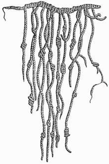
HistoryA Quipu, which is used by the Inca to record numbers.The main article for this section are: History of mathematics
Evolution can be seen as a series of mathematical abstraction which always multiply, or other words of the subject matter of the expansion. ABSTRACT initially, which also applies to many animals, is about numbers: a statement that two apples and two oranges (for example) have the same number.
In addition to knowing how to count physical objects, prehistoric humans also recognize how to count abstract quantities, like time - days, seasons, years. Basic arithmetic (addition, subtraction, multiplication, and division) naturally followed.
The next step requires a writing or other system to record numbers, such as a rope or knotted strings called Quipu used by the Inca to store numerical data. The number system there are many and diverse, the first known written numbers in the manuscript heritage of Ancient Egypt in the Middle Kingdom of Egypt, the Rhind Mathematical Gazette.Maya number system
The use of the most ancient mathematics is in trade, land surveying, painting, and patterns of weaving and recording times and never flourished until the year 3000 BC to advance when the Babylonians and the Ancient Egyptians began using arithmetic, algebra, and geometry for tax calculation and other financial dealings, building and construction, and astronomy. Systematic assessment of mathematics in their own truth began in ancient Greece between 600 and 300 BC.
Math since then promptly widespread, and there is a beneficial interaction between mathematics and science, benefiting both parties. Mathematical discoveries made throughout history and continues today. According to Mikhail B. Sevryuk, in the January 2006 issue of the Bulletin of the American Mathematical Society, "The number of papers and books included in the Mathematical Reviews database since 1940 (the first year of operation of MR) now exceeds 1.9 million, and exceeded 75 thousand articles added to the database each year. Most of the works in this ocean contain new mathematical theorems and their evidence. "Etymology
The word "mathematics" comes from the Ancient Greek language μάθημα (mathema), which means the assessment, learning, science scope narrowed, and technical meanings become "mathematics assessment", even so in ancient times. Adjectives are μαθηματικός (mathēmatikós), relating to the assessment, or studious, more meaningful mathematical away. In particular, μαθηματικὴ τέχνη (mathēmatikḗ tékhnē), in Latin ars mathematica, meant the mathematical art.
The plural form is often used in English, as well as in French les mathématiques (and rarely used as a derivative of the singular la mathématique), refer to the plural form of Latin which tend to be neutral mathematica (Cicero), based on the plural Greek τα μαθηματικά (ta Mathematics), who used Aristotle, which roughly translated means "all things mathematical". But in English, mathematics nouns take singular when used as a verb. Within the range of conversation, mathematics often abbreviated as math in North America and maths elsewhere.
 A Quipu, which is used by the Inca to record numbers
 Maya number system
pure and applied mathematics, and aestheticsSir Isaac Newton (1643-1727), an inventor of infinitesimal calculus.The main article for this section are: The beauty of mathematics
Mathematics arises when it faces complex problems that involve quantity, structure, space, or change. At first, the problems encountered in the trade, land surveying, and later astronomy; now, all science advocated problems studied by mathematicians, and many problems arise within mathematics itself. For example, a physicist Richard Feynman path integral found the formula of quantum mechanics using a combination of mathematical reasoning and physical insight, and today's string theory, a scientific theory that is still growing which seeks membersatukan four fundamental forces of nature, continues to inspire new mathematics.
Some mathematical correspond only in the area that inspired it, and is applied to solve further problems in that region. But often mathematics inspired by the evidence in the region it is useful also in many other areas, and combines common stock of mathematical concepts. The amazing fact that mathematics "purest" often turned to have practical applications is what Eugene Wigner called it "remarkable effectiveness of mathematics to some absurd in Natural Sciences in need of explanation.".
As in most areas of study, the explosion of knowledge in the scientific age has led to specialization in mathematics. One major distinction is between pure mathematics and applied mathematics: most mathematicians focus their research solely on one of this region, and sometimes these choices made early in the course of their undergraduate program. Several areas of applied mathematics have merged with the corresponding traditions outside of mathematics and become a discipline which has its own right, including statistics, operations research, and computer science.
Those with an interest in mathematics often encounter a certain aesthetic aspects in a lot of math. Many mathematicians talk about the elegance of mathematics, aesthetics implied, and the beauty of it. The simplicity and generality appreciated. There is beauty in the simplicity and elegance of the evidence provided, such as Euclid's proof that that there are infinite number of primes, and in an elegant numerical method that the calculation of the rate, the fast Fourier transform. G. H. Hardy in A Mathematician's Apology expressed the belief that aesthetic penganggapan this, in itself, sufficient to support the study of pure mathematics.
Mathematicians often work hard to find evidence that elegant theorems specifically, the quest Paul Erdős often dwell on the type of search root of the "Bible" in which God has written evidence favorite. Kepopularan recreational mathematics is another sign that the excitement often found when someone is able to solve math problems.
Notation, language, and stiffnessLeonhard Euler. Most probably a mathematician who produced findings of all timeThe main article for this section are: mathematical notation
Most of the mathematical notation in use today was not invented until the 16th century. In the 18th century, Euler was responsible for many notations in use today. Modern notation makes mathematics easier for professionals, but beginners often find it as something terrible. Compaction occurs extreme: little emblem contains a wealth of information. Such as musical notation, modern mathematical notation has a strict syntax and encodes information that is perhaps difficult to be written in any other way.
The language of mathematics can also seem difficult for the beginner. Words such as or and only have more precise meanings than in everyday speech. In addition, words such as open and field gives special meaning mathematics. Mathematical jargon includes technical terms such as homeomorphism and terintegralkan. But there is a reason for special notation and this technical jargon: mathematics requires more precision than everyday speech. Mathematicians refer to this precision of language and logic as "tight" or "rigid" (rigor). So, if a word has been interpreted with a certain meaning, then later said it should refer to the earlier meaning. There should not be changed meaning. That is the meaning of "tight" in the language of mathematics.Ketakhinggaan emblem ∞ in some style dish.
The use of language is fundamentally a rigorous mathematical proof properties. Mathematicians want their theorems to follow axioms with the intention of systematic reasoning. This is to prevent the "theorem" which one to take, based on a presumption of failure, where many examples ever appeared in the history of this subject. The level of rigor expected in mathematics are always changing over time: the Greeks want detailed arguments, but at the time of Isaac Newton the methods used kuranglah stiff. Problems inherent in the definitions used Newton would lead to the emergence of careful analysis and formal proof in the 19th century. Today, mathematicians continue to argue about computer-assisted proof. Because large calculations very difficult examined, the evidence that might not be quite stiff.
Axiom according to traditional thinking is "the truth which is proof in itself", but the concept is triggering the problem. At the formal level, an axiom is just a piece of string emblem, which only has meaning implicit in all formulas terturunkan context of a system of axioms. This is the purpose Hilbert's program to put all of mathematics in an axiom solid basis, but according to Gödel's Theorem ketaklengkapan every axiom system (strong enough) have formulas that can not be determined; and because of that a final aksiomatisasi in mathematics is impossible. However, mathematics is often imagined (in a formal context) nothing but set theory in some aksiomatisasi, with the understanding that each statement or mathematical proofs can be packed into a formula of set theory.
 Coat of infinite ∞ in some style dish.
Introduction
A set is a collection of elements, and may be described in many ways. One way is simply to list all of its elements; for example, the set consisting of the integers 3, 4, and 5 may be denoted {3, 4, 5}. This is only effective for small sets, however; for larger sets, this would be time-consuming and error-prone. Instead of listing every single element, sometimes an ellipsis ("...") is used, if the writer believes that the reader can easily guess what is missing; for example, {1, 2, 3, ..., 100} presumably denotes the set of integers from 1 to 100. Even in this case, however, it is still possible to list all the elements, because the set is finite.Some sets are infinite; these sets have more than n elements for any integer n. For example, the set of natural numbers, denotable by {0, 1, 2, 3, 4, 5, ...}, has infinitely many elements, and we cannot use any normal number to give its size. Nonetheless, it turns out that infinite sets do have a well-defined notion of size (or more properly, of cardinality, which is the technical term for the number of elements in a set), and not all infinite sets have the same cardinality.

Bijective mapping from integer to even numbers
However, not all infinite sets have the same cardinality. For example, Georg Cantor (who introduced this concept) demonstrated that the real numbers cannot be put into one-to-one correspondence with the natural numbers (non-negative integers), and therefore that the set of real numbers has a greater cardinality than the set of natural numbers.
A set is countable if: (1) it is finite, or (2) it has the same cardinality (size) as the set of natural numbers. Equivalently, a set is countable if it has the same cardinality as some subset of the set of natural numbers. Otherwise, it is uncountable.
Formal overview without details
By definition a set S is countable if there exists an injective function f : S → N from S to the natural numbers N = {0, 1, 2, 3, ...}.It might seem natural to divide the sets into different classes: put all the sets containing one element together; all the sets containing two elements together; ...; finally, put together all infinite sets and consider them as having the same size. This view is not tenable, however, under the natural definition of size.
To elaborate this we need the concept of a bijection. Although a "bijection" seems a more advanced concept than a number, the usual development of mathematics in terms of set theory defines functions before numbers, as they are based on much simpler sets. This is where the concept of a bijection comes in: define the correspondence
- a ↔ 1, b ↔ 2, c ↔ 3
We now generalize this situation and define two sets as of the same size if (and only if) there is a bijection between them. For all finite sets this gives us the usual definition of "the same size". What does it tell us about the size of infinite sets?
Consider the sets A = {1, 2, 3, ... }, the set of positive integers and B = {2, 4, 6, ... }, the set of even positive integers. We claim that, under our definition, these sets have the same size, and that therefore B is countably infinite. Recall that to prove this we need to exhibit a bijection between them. But this is easy, using n ↔ 2n, so that
- 1 ↔ 2, 2 ↔ 4, 3 ↔ 6, 4 ↔ 8, ....
Likewise, the set of all ordered pairs of natural numbers is countably infinite, as can be seen by following a path like the one in the picture:

The Cantor pairing function assigns one natural number to each pair of natural numbers
- 0 ↔ (0,0), 1 ↔ (1,0), 2 ↔ (0,1), 3 ↔ (2,0), 4 ↔ (1,1), 5 ↔ (0,2), 6 ↔ (3,0) ....
Interestingly: if you treat each pair as being the numerator and denominator of a vulgar fraction, then for every positive fraction, we can come up with a distinct number corresponding to it. This representation includes also the natural numbers, since every natural number is also a fraction N/1. So we can conclude that there are exactly as many positive rational numbers as there are positive integers. This is true also for all rational numbers, as can be seen below.
Theorem: The Cartesian product of finitely many countable sets is countable.
This form of triangular mapping recursively generalizes to vectors of finitely many natural numbers by repeatedly mapping the first two elements to a natural number. For example, (0,2,3) maps to (5,3), which maps to 39.
Sometimes more than one mapping is useful. This is where you map the set you want to show is countably infinite onto another set—and then map this other set to the natural numbers. For example, the positive rational numbers can easily be mapped to (a subset of) the pairs of natural numbers because p/q maps to (p, q).
What about infinite subsets of countably infinite sets? Do these have fewer elements than N?
Theorem: Every subset of a countable set is countable. In particular, every infinite subset of a countably infinite set is countably infinite.
For example, the set of prime numbers is countable, by mapping the n-th prime number to n:
- 2 maps to 1
- 3 maps to 2
- 5 maps to 3
- 7 maps to 4
- 11 maps to 5
- 13 maps to 6
- 17 maps to 7
- 19 maps to 8
- 23 maps to 9
- ...
Theorem: Z (the set of all integers) and Q (the set of all rational numbers) are countable.
In a similar manner, the set of algebraic numbers is countable.
These facts follow easily from a result that many individuals find non-intuitive.
Theorem: Any finite union of countable sets is countable.
With the foresight of knowing that there are uncountable sets, we can wonder whether or not this last result can be pushed any further. The answer is "yes" and "no", we can extend it, but we need to assume a new axiom to do so.
Theorem: (Assuming the axiom of countable choice) The union of countably many countable sets is countable.
For example, given countable sets a, b, c, ...

Enumeration for countable number of countable sets
- a0 maps to 0
- a1 maps to 1
- b0 maps to 2
- a2 maps to 3
- b1 maps to 4
- c0 maps to 5
- a3 maps to 6
- b2 maps to 7
- c1 maps to 8
- d0 maps to 9
- a4 maps to 10
- ...
Also note that we need the axiom of countable choice to index all the sets a, b, c, ... simultaneously.
Theorem: The set of all finite-length sequences of natural numbers is countable.
This set is the union of the length-1 sequences, the length-2 sequences, the length-3 sequences, each of which is a countable set (finite Cartesian product). So we are talking about a countable union of countable sets, which is countable by the previous theorem.
Theorem: The set of all finite subsets of the natural numbers is countable.
If you have a finite subset, you can order the elements into a finite sequence. There are only countably many finite sequences, so also there are only countably many finite subsets.
The following theorem gives equivalent formulations in terms of a bijective function or a surjective function. A proof of this result can be found in Lang's text.
(Basic) Theorem: Let S be a set. The following statements are equivalent:
- S is countable, i.e. there exists an injective function f : S → N.
- Either S is empty or there exists a surjective function g : N → S.
- Either S is finite or there exists a bijection h : N → S.
- If the function f : S → T is injective and T is countable then S is countable.
- If the function g : S → T is surjective and S is countable then T is countable.
Proposition: The set P(N) is not countable; i.e. it is uncountable.
For an elaboration of this result see Cantor's diagonal argument.
The set of real numbers is uncountable (see Cantor's first uncountability proof), and so is the set of all infinite sequences of natural numbers.
Some technical details
The proofs of the statements in the above section rely upon the existence of functions with certain properties. This section presents functions commonly used in this role, but not the verifications that these functions have the required properties. The Basic Theorem and its Corollary are often used to simplify proofs. Observe that N in that theorem can be replaced with any countably infinite set.Proposition: Any finite set is countable.
Proof: By definition, there is a bijection between a non-empty finite set S and the set {1, 2, ..., n} for some positive natural number n. This function is an injection from S into N.
Proposition: Any subset of a countable set is countable .
Proof: The restriction of an injective function to a subset of its domain is still injective.
Proposition: If S is a countable set and x ∉ S, then S ∪ {x} is countable.
Proof: Let f: S → N be an injection. Define g: S ∪ {x} → N by g(x) = 0 and g(y) = f(y) + 1 for all y in S. This function g is an injection.
Proposition: If A and B are countable sets then A ∪ B is countable.
Proof: Let f: A → N and g: B → N be injections. Define a new injection h: A ∪ B → N by h(x) = 2f(x) if x is in A and h(x) = 2g(x) + 1 if x is in B but not in A.
Proposition: The Cartesian product of two countable sets A and B is countable.
Proof: Observe that N × N is countable as a consequence of the definition because the function f : N × N → N given by f(m, n) = 2m3n is injective. It then follows from the Basic Theorem and the Corollary that the Cartesian product of any two countable sets is countable. This follows because if A and B are countable there are surjections f : N → A and g : N → B. So
- f × g : N × N → A × B
Proposition: The integers Z are countable and the rational numbers Q are countable.
Proof: The integers Z are countable because the function f : Z → N given by f(n) = 2n if n is non-negative and f(n) = 3− n if n is negative, is an injective function. The rational numbers Q are countable because the function g : Z × N → Q given by g(m, n) = m/(n + 1) is a surjection from the countable set Z × N to the rationals Q.
Proposition: If An is a countable set for each n in N then the union of all An is also countable.
Proof: This is a consequence of the fact that for each n there is a surjective function gn : N → An and hence the function

A topological proof for the uncountability of the real numbers is described at finite intersection property.
Minimal model of set theory is countable
If there is a set that is a standard model (see inner model) of ZFC set theory, then there is a minimal standard model (see Constructible universe). The Löwenheim-Skolem theorem can be used to show that this minimal model is countable. The fact that the notion of "uncountability" makes sense even in this model, and in particular that this model M contains elements that are:- subsets of M, hence countable,
- but uncountable from the point of view of M,
The minimal standard model includes all the algebraic numbers and all effectively computable transcendental numbers, as well as many other kinds of numbers.
Total orders
Countable sets can be totally ordered in various ways, e.g.:- Well orders (see also ordinal number):
- The usual order of natural numbers (0, 1, 2, 3, 4, 5, ...)
- The integers in the order (0, 1, 2, 3, ...; −1, −2, −3, ...)
- Other (not well orders):
- The usual order of integers (..., −3, −2, −1, 0, 1, 2, 3, ...)
- The usual order of rational numbers (Cannot be explicitly written as an ordered list!)
X . IIIIIII Uncountable set
"Uncountable" redirects here. For the linguistic concept, see Uncountable noun.
In mathematics, an uncountable set (or uncountably infinite set) is an infinite set that contains too many elements to be countable. The uncountability of a set is closely related to its cardinal number: a set is uncountable if its cardinal number is larger than that of the set of all natural numbers.Characterizations
There are many equivalent characterizations of uncountability. A set X is uncountable if and only if any of the following conditions holds:- There is no injective function from X to the set of natural numbers.
- X is nonempty and for every ω-sequence of elements of X, there exist at least one element of X not included in it. That is, X is nonempty and there is no surjective function from the natural numbers to X.
- The cardinality of X is neither finite nor equal to
- The set X has cardinality strictly greater than
Properties
- If an uncountable set X is a subset of set Y, then Y is uncountable.
Examples
The best known example of an uncountable set is the set R of all real numbers; Cantor's diagonal argument shows that this set is uncountable. The diagonalization proof technique can also be used to show that several other sets are uncountable, such as the set of all infinite sequences of natural numbers and the set of all subsets of the set of natural numbers. The cardinality of R is often called the cardinality of the continuum and denoted by c, or, or (beth-one).The Cantor set is an uncountable subset of R. The Cantor set is a fractal and has Hausdorff dimension greater than zero but less than one (R has dimension one). This is an example of the following fact: any subset of R of Hausdorff dimension strictly greater than zero must be uncountable.
Another example of an uncountable set is the set of all functions from R to R. This set is even "more uncountable" than R in the sense that the cardinality of this set is
(beth-two), which is larger than .A more abstract example of an uncountable set is the set of all countable ordinal numbers, denoted by Ω or ω1. The cardinality of Ω is denoted
(aleph-one). It can be shown, using the axiom of choice, that is the smallest uncountable cardinal number. Thus either , the cardinality of the reals, is equal to or it is strictly larger. Georg Cantor was the first to propose the question of whether is equal to . In 1900, David Hilbert posed this question as the first of his 23 problems. The statement that is now called the continuum hypothesis and is known to be independent of the Zermelo–Fraenkel axioms for set theory (including the axiom of choice).Without the axiom of choice
Main article: Dedekind-infinite set
Without the axiom of choice, there might exist cardinalities incomparable to (namely, the cardinalities of Dedekind-finite
infinite sets). Sets of these cardinalities satisfy the first three
characterizations above but not the fourth characterization. Because
these sets are not larger than the natural numbers in the sense of
cardinality, some may not want to call them uncountable.If the axiom of choice holds, the following conditions on a cardinal
are equivalent:and
, where
and
is least initial ordinal greater than


X . IIIIIIII Interpretation ( Model Theory )
In model theory, interpretation of a structure M in another structure N (typically of a different signature) is a technical notion that approximates the idea of representing M inside N. For example every reduct or definitional expansion of a structure N has an interpretation in N.
Many model-theoretic properties are preserved under interpretability. For example if the theory of N is stable and M is interpretable in N, then the theory of M is also stable.
Definition
An interpretation of M in N with parameters (or without parameters, respectively) is a pair where n is a natural number and is a surjective map from a subset of Nn onto M such that the -preimage (more precisely the -preimage) of every set X ⊆ Mk definable in M by a first-order formula without parameters is definable (in N) by a first-order formula with parameters (or without parameters, respectively). Since the value of n for an interpretation is often clear from context, the map itself is also called an interpretation.To verify that the preimage of every definable (without parameters) set in M is definable in N (with or without parameters), it is sufficient to check the preimages of the following definable sets:
- the domain of M;
- the diagonal of M;
- every relation in the signature of M;
- the graph of every function in the signature of M.
Bi-interpretability
If L, M and N are three structures, L is interpreted in M, and M is interpreted in N, then one can naturally construct a composite interpretation of L in N. If two structures M and N are interpreted in each other, then by combining the interpretations in two possible ways, one obtains an interpretation of each of the two structures in itself. This observation permits one to define an equivalence relation among structures, reminiscent of the homotopy equivalence among topological spaces.Two structures M and N are bi-interpretable if there exists an interpretation of M in N and an interpretation of N in M such that the composite interpretations of M in itself and of N in itself are definable in M and in N, respectively (the composite interpretations being viewed as operations on M and on N).
Example
The partial map f from Z × Z onto Q which maps (x, y) to x/y provides an interpretation of the field Q of rational numbers in the ring Z of integers (to be precise, the interpretation is (2, f)). In fact, this particular interpretation is often used to define the rational numbers. To see that it is an interpretation (without parameters), one needs to check the following preimages of definable sets in Q:- the preimage of Q is defined by the formula φ(x, y) given by ¬ (y = 0);
- the preimage of the diagonal of Q is defined by the formula φ(x1, y1, x2, y2) given by x1 × y2 = x2 × y1;
- the preimages of 0 and 1 are defined by the formulas φ(x, y) given by x = 0 and x = y;
- the preimage of the graph of addition is defined by the formula φ(x1, y1, x2, y2, x3, y3) given by x1×y2×y3 + x2×y1×y3 = x3×y1×y2;
- the preimage of the graph of multiplication is defined by the formula φ(x1, y1, x2, y2, x3, y3) given by x1×x2×y3 = x3×y1×y2.
X . IIIIIIIII Object Object Mathematic
Mathematics (from Greek: μαθηματικά - Mathematics) is the study of quantity, structure, space, and change. The mathematicians are looking for a variety of patterns, formulate new conjectures, and establish truth by rigorous deduction method derived from axioms and definitions coincide.
There is a debate about whether mathematical objects such as numbers and points already exist in the universe, so found, or a human creation. A mathematician Benjamin Peirce called the mathematics as "the science that describes the important conclusions". However, despite the fact that mathematics is very useful in life, the development of science and technology, to efforts to preserve the natural, mathematical life in the world of ideas, not in reality or reality. Appropriately, Albert Einstein stated that "as far as the laws of mathematics refer to reality, they are not certain; and as far as they are certain, they do not refer to reality." The meaning of "Mathematics do not refer to reality" convey the message that a mathematical idea was ideal and sterile or protected from human influence. Interestingly, freedom of reality and the human impact of this will actually allow concluding statement that the universe is a mathematical structure, according to Max Tegmark. If we believe that the reality beyond this universe must be free from human influence, it must be the mathematical structure of the universe was that.
Through the use of abstraction and logical reasoning, mathematics evolved from counting, calculation, measurement, and the systematic study of the shapes and motions of physical objects. Practical mathematics manifests in human activities since written records exist. Rigorous mathematical arguments first appeared in Greek mathematics, most notably in Euclid, Elements.
Mathematics continued to develop, for example in China in 300 BC, in India in the year 100 AD, and in Arabia in 800 AD, until the Renaissance, when new findings mathematics interacting with new scientific discoveries that led to a rapid increase in the pace of invention mathematics that continues today.
Today, mathematics is used throughout the world as an essential tool in many fields, including natural science, engineering, medicine / medical, and social sciences such as economics, and psychology. Applied mathematics, the branch of mathematics which covers the application of mathematical knowledge to other fields, inspires and makes use of new mathematical discoveries and sometimes leads to the development of scientific disciplines are entirely new, such as statistics and game theory.
The mathematician also wrestled in pure mathematics, or mathematics for the development of mathematics itself. They sought to answer the questions that arise in his mind, although its application is not yet known. However, in reality a lot of mathematical ideas were very abstract and previously unknown relevance to life, suddenly found its application. The development of mathematics (pure) can precede or preceded needs in life. Practical application of mathematical ideas that become the background of the emergence of pure mathematics are often discovered later.
Etymology
The word "mathematics" comes from the Ancient Greek language μάθημα (mathema), which means the assessment, learning, science scope narrowed, and technical meanings become "mathematics assessment", even so in ancient times. Adjectives are μαθηματικός (mathēmatikós), relating to the assessment, or studious, more meaningful mathematical away. In particular, μαθηματικὴ τέχνη (mathēmatikḗ tékhnē), in Latin ars mathematica, meant the mathematical art.
The plural form is often used in English, as well as in French les mathématiques (and rarely used as a derivative of the singular la mathématique), refer to the plural form of Latin which tend to be neutral mathematica (Cicero), based on the plural Greek τα μαθηματικά (ta Mathematics), who used Aristotle, which roughly translated means "all things mathematical". But in English, mathematics nouns take singular when used as a verb. Within the range of conversation, mathematics often abbreviated as math in North America and maths elsewhere.
HistoryA Quipu, which is used by the Inca to record numbers.The main article for this section are: History of mathematics
Evolution can be seen as a series of mathematical abstraction which always multiply, or other words of the subject matter of the expansion. ABSTRACT initially, which also applies to many animals, is about numbers: a statement that two apples and two oranges (for example) have the same number.
In addition to knowing how to count physical objects, prehistoric humans also recognize how to count abstract quantities, like time - days, seasons, years. Basic arithmetic (addition, subtraction, multiplication, and division) naturally followed.
The next step requires a writing or other system to record numbers, such as a rope or knotted strings called Quipu used by the Inca to store numerical data. The number system there are many and diverse, the first known written numbers in the manuscript heritage of Ancient Egypt in the Middle Kingdom of Egypt, the Rhind Mathematical Gazette.Maya number system
The use of the most ancient mathematics is in trade, land surveying, painting, and patterns of weaving and recording times and never flourished until the year 3000 BC to advance when the Babylonians and the Ancient Egyptians began using arithmetic, algebra, and geometry for tax calculation and other financial dealings, building and construction, and astronomy. Systematic assessment of mathematics in their own truth began in ancient Greece between 600 and 300 BC.
Math since then promptly widespread, and there is a beneficial interaction between mathematics and science, benefiting both parties. Mathematical discoveries made throughout history and continues today. According to Mikhail B. Sevryuk, in the January 2006 issue of the Bulletin of the American Mathematical Society, "The number of papers and books included in the Mathematical Reviews database since 1940 (the first year of operation of MR) now exceeds 1.9 million, and exceeded 75 thousand articles added to the database each year. Most of the works in this ocean contain new mathematical theorems and their evidence. "Etymology
The word "mathematics" comes from the Ancient Greek language μάθημα (mathema), which means the assessment, learning, science scope narrowed, and technical meanings become "mathematics assessment", even so in ancient times. Adjectives are μαθηματικός (mathēmatikós), relating to the assessment, or studious, more meaningful mathematical away. In particular, μαθηματικὴ τέχνη (mathēmatikḗ tékhnē), in Latin ars mathematica, meant the mathematical art.
The plural form is often used in English, as well as in French les mathématiques (and rarely used as a derivative of the singular la mathématique), refer to the plural form of Latin which tend to be neutral mathematica (Cicero), based on the plural Greek τα μαθηματικά (ta Mathematics), who used Aristotle, which roughly translated means "all things mathematical". But in English, mathematics nouns take singular when used as a verb. Within the range of conversation, mathematics often abbreviated as math in North America and maths elsewhere.
A Quipu, which is used by the Inca to record numbers Maya number system pure and applied mathematics, and aestheticsSir Isaac Newton (1643-1727), an inventor of infinitesimal calculus.The main article for this section are: The beauty of mathematics
Mathematics arises when it faces complex problems that involve quantity, structure, space, or change. At first, the problems encountered in the trade, land surveying, and later astronomy; now, all science advocated problems studied by mathematicians, and many problems arise within mathematics itself. For example, a physicist Richard Feynman path integral found the formula of quantum mechanics using a combination of mathematical reasoning and physical insight, and today's string theory, a scientific theory that is still growing which seeks membersatukan four fundamental forces of nature, continues to inspire new mathematics.
Some mathematical correspond only in the area that inspired it, and is applied to solve further problems in that region. But often mathematics inspired by the evidence in the region it is useful also in many other areas, and combines common stock of mathematical concepts. The amazing fact that mathematics "purest" often turned to have practical applications is what Eugene Wigner called it "remarkable effectiveness of mathematics to some absurd in Natural Sciences in need of explanation.".
As in most areas of study, the explosion of knowledge in the scientific age has led to specialization in mathematics. One major distinction is between pure mathematics and applied mathematics: most mathematicians focus their research solely on one of this region, and sometimes these choices made early in the course of their undergraduate program. Several areas of applied mathematics have merged with the corresponding traditions outside of mathematics and become a discipline which has its own right, including statistics, operations research, and computer science.
Those with an interest in mathematics often encounter a certain aesthetic aspects in a lot of math. Many mathematicians talk about the elegance of mathematics, aesthetics implied, and the beauty of it. The simplicity and generality appreciated. There is beauty in the simplicity and elegance of the evidence provided, such as Euclid's proof that that there are infinite number of primes, and in an elegant numerical method that the calculation of the rate, the fast Fourier transform. G. H. Hardy in A Mathematician's Apology expressed the belief that aesthetic penganggapan this, in itself, sufficient to support the study of pure mathematics.
Mathematicians often work hard to find evidence that elegant theorems specifically, the quest Paul Erdős often dwell on the type of search root of the "Bible" in which God has written evidence favorite. Kepopularan recreational mathematics is another sign that the excitement often found when someone is able to solve math problems.
Notation, language, and stiffnessLeonhard Euler. Most probably a mathematician who produced findings of all timeThe main article for this section are: mathematical notation
Most of the mathematical notation in use today was not invented until the 16th century. In the 18th century, Euler was responsible for many notations in use today. Modern notation makes mathematics easier for professionals, but beginners often find it as something terrible. Compaction occurs extreme: little emblem contains a wealth of information. Such as musical notation, modern mathematical notation has a strict syntax and encodes information that is perhaps difficult to be written in any other way.
The language of mathematics can also seem difficult for the beginner. Words such as or and only have more precise meanings than in everyday speech. In addition, words such as open and field gives special meaning mathematics. Mathematical jargon includes technical terms such as homeomorphism and terintegralkan. But there is a reason for special notation and this technical jargon: mathematics requires more precision than everyday speech. Mathematicians refer to this precision of language and logic as "tight" or "rigid" (rigor). So, if a word has been interpreted with a certain meaning, then later said it should refer to the earlier meaning. There should not be changed meaning. That is the meaning of "tight" in the language of mathematics.Ketakhinggaan emblem ∞ in some style dish.
The use of language is fundamentally a rigorous mathematical proof properties. Mathematicians want their theorems to follow axioms with the intention of systematic reasoning. This is to prevent the "theorem" which one to take, based on a presumption of failure, where many examples ever appeared in the history of this subject. The level of rigor expected in mathematics are always changing over time: the Greeks want detailed arguments, but at the time of Isaac Newton the methods used kuranglah stiff. Problems inherent in the definitions used Newton would lead to the emergence of careful analysis and formal proof in the 19th century. Today, mathematicians continue to argue about computer-assisted proof. Because large calculations very difficult examined, the evidence that might not be quite stiff.
Axiom according to traditional thinking is "the truth which is proof in itself", but the concept is triggering the problem. At the formal level, an axiom is just a piece of string emblem, which only has meaning implicit in all formulas terturunkan context of a system of axioms. This is the purpose Hilbert's program to put all of mathematics in an axiom solid basis, but according to Gödel's Theorem ketaklengkapan every axiom system (strong enough) have formulas that can not be determined; and because of that a final aksiomatisasi in mathematics is impossible. However, mathematics is often imagined (in a formal context) nothing but set theory in some aksiomatisasi, with the understanding that each statement or mathematical proofs can be packed into a formula of set theory.
Mathematics as a scienceCarl Friedrich Gauss, regards itself as the "prince of mathematicians", and said that mathematics as "the queen of Science".
Carl Friedrich Gauss said that mathematics as "the queen of Science". In their original languages, Latin Regina scientiarum, as well as in German Königin der Wissenschaften, the word corresponding to science means (field) knowledge. Clearly, even this original meaning in English, and there is no doubt that mathematics in this context is a science. Specialization which narrowed the meaning of being natural science is the latter period. When one looks at the science is confined to the world of physics, then mathematics, or at least pure mathematics, not science.
Albert Einstein stated that "as far as the laws of mathematics refer to reality, they are not certain; and as far as they are certain, they do not refer to reality."
Many philosophers believe that mathematics can not be proven nor refuted by experiments, and thus not a science per the definition of Karl Popper. But in the important work of the 1930s on mathematical logic showed that mathematics can not be reduced to logic, and Karl Popper concluded that "most mathematical theories, such as physics and biology, are hypothetical-deductive: therefore the math becomes more close to the natural science hypothesis-the hypothesis is a conjecture (conjecture), rather than as a novelty. " The other sage, say Imre Lakatos, have applied a counterfeit version of the mathematics itself.
A review of the alternative is that certain scientific fields (such as theoretical physics) are mathematics with axioms that are intended so that corresponds with reality. In fact, a theoretical physicist, John Ziman, proposed that science is public knowledge and thus includes mathematics. In some cases, sharing with many mathematical science of physics, namely logical excavation impacts of some contention. Intuition and experimentation also play an important role in the formulation of conjectures-conjectures, be it in mathematics, as well as in the sciences (more).
Mathematical experiment continues to grow flowers, given its importance in mathematics, and computation and simulation play an increasingly powerful role, be it in science, as well as in mathematics, weakening the objection that is where the math does not use the scientific method. In his book published in 2002, A New Kind of Science, Stephen Wolfram postulates that computational mathematics deserves to be explored empirically as a scientific field in the right / truth itself.
The opinions of mathematicians to this there are various kinds. Many mathematicians feel that to call their area a science is tantamount to lowering interest aesthetic side, and its history in the traditional seven liberal arts; others felt that ignoring this link to knowledge is tantamount to twirling a blind eye to the fact that the interface between mathematics and its applications in science and engineering had driven much development in mathematics.
One way is played by differences in point of view is in the philosophical debate whether mathematics is created (as in art) or discovered (as in science). It is reasonable for the university when it was divided into sections that include the department of Science and Mathematics, it indicates that the fields are seen allied but they do not like the two sides of the coin. On a practical level, mathematicians usually grouped together scientists at the level of harsh, but separated at the final stage. This is one of the many things to consider in the philosophy of mathematics.
Mathematics awards are generally maintained in order to remain separate from equality with science. The valuable award in mathematics is the Fields Medal (medal field), commenced in 1936 and is now held every four years. This award is often considered equivalent to the Nobel Prize in science.
Wolf Prize in Mathematics, instituted in 1978, recognizes the past achievements, and other major international award, the Abel Prize, was introduced in 2003. It was awarded for a special segment of the work, can be a renewal, or a prominent problem resolution within the established field.
A famous list contains 23 open problems, called "Hilbert problems", compiled in 1900 by German mathematician David Hilbert. This list won persulangan widely among mathematicians, and at least nine of the problems are now solved.
A new list of seven important problems, titled "Millennium Prize Problems", published in 2000. Solving these problems each prize of US $ 1 million, and only one (the Riemann hypothesis) that experienced a doubling in the problems of Hilber
The disciplines in mathematics major at first appear because of the need for calculations in commerce, to understand the relationship antarbilangan, to measure land and to predict astronomical events. Four of these needs can be roughly attributed to divisions into the rough math assessment scale, structure, space, and change (ie arithmetic, algebra, geometry, and analysis). In addition to that subject, there are also divisions dedicated to links-links excavation from the heart of mathematics to fields other: to logic, to set theory (basic), to mathematics empirically from various kinds of knowledge (applied mathematics), and newer is rigid assessment to be uncertainty.magnitude
Assessment begins with the massive numbers, the first natural numbers and integers ( "all numbers") and the arithmetic operations in the numbers, which dipersifatkan in arithmetic. The properties of the integers deeper studied in number theory, where it comes from popular results as Fermat's Last Theorem. Number theory also holds two unsolved problems: the twin prime conjecture and Goldbach conjecture.
Because the number system is further developed, the integers are recognized as a subset of the rational numbers ( "fractions"). While fractions are in real numbers, which are used to represent continuous quantities. Generalized real numbers into complex numbers. This is the first step on the ladder of numbers which moved to include quaternion and octonion. Attention to the natural numbers also leads to transfinit numbers, which formalize the concept of enumeration ketakhinggaan. Other regions of this study is size, which leads to the cardinal numbers and then on the other ketakhinggaan conception: alef numbers, which allow meaningful comparison of the size of the sets are infinitely large.
 An abacus, a simple calculating tool used since ancient times.
 Room
Assessment begins with the geometry of space - in particular, Euclidean geometry. Trigonometry combines space and numbers, and includes the famous Pythagorean Theorem. Modern assessment of space memperumum these ideas to include higher-dimensional geometry, non-Euclidean geometries (which play an important role in general relativity) and topology. Magnitude and space plays an important role in analytic geometry, differential geometry, algebra and geometry. Within differential geometry are the concepts of fiber bundles and calculus folds.
Inside there is an explanation algebraic geometry geometrical objects as set completion polynomial equations, combining the concepts of quantity and space, and also study topological groups, which combine structure and space. Group lie commonly used to study space, structure, and change. Topology in many ramifications may be the biggest growth area in 20th century mathematics, and include the Poincaré conjecture which has long existed and the four-color theorem, whose only "successfully" proved by a computer, and has not been proved by humans manually.
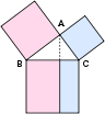


Geometric Trigonometric differensial geometric Topology fractal geometric
Change
Understand and explain the changes are common themes in the natural sciences, and calculus has evolved as a full-power to investigate. Functions arise here, as an important concept to explain the magnitude of the change. Rigid assessment of real numbers and functions in the form of real change is known as real analysis, with complex analysis the equivalent field for the complex numbers.
Riemann hypothesis, one of the most fundamental open problems in mathematics, depicted from complex analysis. Functional analysis focusing on the function room (typically infinite-dimensional). One of many applications of functional analysis is quantum mechanics.
Many problems naturally leads to a relationship between the magnitude and rate of change, and is studied as differential equations. Many symptoms in nature can be explained using a dynamical system; chaos theory (chaos correct the streets where many of these systems exhibit deterministic behavior that still can not be guessed.


Calculus vector calculus differential equation dinamic system


Chaos Theory Complex analysis
Structure
Many mathematical objects, such as sets of numbers and functions, exhibit internal structure. The structural properties of these objects are investigated in the study group, rink, field and other abstract systems, which themselves are objects as well. This is the field of abstract algebra. An important concept here that vector, generalized into a vector space, and studied in linear algebra. Vector Assessment combines three basic areas of mathematics: quantity, structure, and space. Vector calculus expands the field into four basic areas, namely the change. Tensor calculus and behavior reviewing kesetangkupan rotated vector. A number of ancient problems concerning compass and straight-line construction finally resolved by Galois theory.
Many mathematical objects, such as sets of numbers and functions, exhibit internal structure. The structural properties of these objects are investigated in the study group, rink, field and other abstract systems, which themselves are objects as well. This is the field of abstract algebra. An important concept here that vector, generalized into a vector space, and studied in linear algebra. Vector Assessment combines three basic areas of mathematics: quantity, structure, and space. Vector calculus expands the field into four basic areas, namely the change. Tensor calculus and behavior reviewing kesetangkupan rotated vector. A number of ancient problems concerning compass and straight-line construction finally resolved by Galois theory.


Algebraic theory abstract algebraic theory group theory order
Basic and philosophy
To clarify the foundations of mathematics, the field of mathematical logic and set theory were developed, as well as category theory which is still being developed. The compound word "crisis basis" explains searches rigid base for mathematics taking place in the decade of the 1900s until the 1930s. [28] Ketaksetujuan some of the fundamentals of mathematics continues today. Basic crunch triggered by a number of later conflicts at that time, including the controversy Cantor set theory and the Brouwer-Hilbert controversy.
Mathematical Logic payed by putting mathematics on a rigid axiomatic framework, and studying the results of that framework. Mathematical logic is home to the second ketaklengkapan Gödel theory, perhaps the result of the most celebrated in the world of logic, which (informally) constitute a formal system that contains basic arithmetic, if sound (meaning all theorems that can be proven are true), then tak- complete (meaning there are true theorems which can not be proven in the system).
Gödel showed how to construct, set any theoretical number given axioms, a formal statement in the logic that is a true number-a theoretical fact, but it does not follow that the axioms. Therefore, there is no formal system is a true aksiomatisasi number theory entirely. Modern logic is divided into recursion theory, model theory, and proof theory, and adrift close to theoretical computer science.


Mathematical Logic set theory category theory
discrete mathematics
Discrete mathematics is the common name for the field of mathematics most useful in theoretical computer science. This includes computability theory, computational complexity theory, and information theory. Computability theory examine the limitations of various theoretical models of the computer, including the most powerful known model - the Turing machine.
Complexity theory is the study tractability by computer; some problems, although theoretically solvable by computer, but quite expensive in terms of time and space, can not be done in practice, even with the rapid advance of computer hardware. Pamungkas, information theory to focus on how much data can be stored on a given medium, and therefore with regard to concepts such as compaction and entropy.
As a relatively new field, discrete mathematics has a number of fundamental open problems. The most famous is the problem of "P = NP?", One of the Millennium Prize Problems.


Combinatorics theory of computation cryptography graph theory
applied mathematics
Applied mathematics with regard to the use of abstract mathematical tools to solve concrete problems in science, business, and other areas. An important field in applied mathematics is statistics, which uses probability theory as a tool and allows the description, analysis, and forecasting symptoms where chance plays an important role. Most experiments, surveys and observational studies require statistics. (But many statisticians, do not regard themselves as a mathematician, but rather as an allied group.)
Numerical analysis investigates computational methods for solving mathematical problems efficiently is usually too large for human numerical capacity, numerical analysis involves assessment of rounding errors or other sources of error in computation.
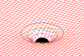

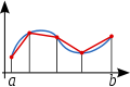

Physical mathematic fluid mechanic numerical analysis optimation


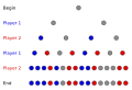
Probability theory statistica finance mathematic game theory

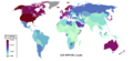
Mathematic biology mathematic chemistry economic mathematic control theory
X . IIIIIIIIIII Calculator and Computer
totalizer
Totalizer or Calculator is a tool to calculate from simple calculations such as addition, subtraction, multiplication and division up to the scientific calculator that can calculate a specific mathematical formula. In development now, the calculator is often included as an additional function than computers, mobile phones, and even watches.
Totalizer or Calculator is a tool to calculate from simple calculations such as addition, subtraction, multiplication and division up to the scientific calculator that can calculate a specific mathematical formula. In development now, the calculator is often included as an additional function than computers, mobile phones, and even watches.


Computers are tools used to process the data according to the procedures that have been formulated. The
word computer was originally used to describe people who perkerjaannya
perform arithmetic calculations, with or without tools, but the meaning
of the word is then transferred to the machine itself. Originally, the processing of information is almost exclusively
related to arithmetical problems, but modern computers are used for many
tasks unrelated to mathematics.
In the sense that there are tools such as slide rules, mechanical calculators types ranging from abacus and so on, until all contemporary electronic computers. The term better suited for a broad sense such as "computer" is "that process information" or "information processing systems." Over the years there have been several different meanings in the word "computer", and several different words are now referred to as the computer.
Said computer once commonly used to define people who perform arithmetic calculations, with or without auxiliary engine. According to Barnhart Concise Dictionary of Etymology, the word is used in English in 1646 as the word for "people who count" and then before 1897 is also used as a "mechanical calculators". During World War II, the word refers to female workers US and British job was to calculate artillery street war with the machine count.
Charles Babbage designed one of the first calculating machine called the analytical engine. In addition, a variety of simple mechanical devices such as slide rule also has to be said as a computer.
 Parts of the Personal Computer.
1: Monitor
2: Board parent
3: Processing
4: Slot ATA
5: Random Access Memory (MAA)
6: PCI Slot
7: Power supply
8: optical disc drive
9: Hard disks
10: Keyboard
11: Mouse
Nevertheless, the above definition includes many specialized tools that can only take into account one or several functions. When considering modern computers, characteristic that most distinguishes them from a computing tool History is the right programming, all computers can emulate nature whatsoever (though perhaps limited by the storage capacity and at different speeds), and, it is believed that a machine could now emulate computing tools that will be created humans in the future (although undoubtedly slower). In a sense, the limits of this ability is a useful test for recognizing computer "general purpose" of a special purpose tool that early. The definition of "general intent" can be formulated into a condition that an engine should be able to emulate the universal Turing machine. The machine that gets this definition is known as a Turing-complete, and which first appeared in 1940 in the midst of worldwide development. See the history of computing article for more detail this period.embedded computers
About 20 years ago, many household appliance, particularly a panel of video games also include mobile phones, video cassette recorders, PDA's and a lot of in the household, industrial, automotive, and other electronic devices, all contain electronic circuits as a qualified computer Turing-complete on top (with a note that the program of the tool is often made directly on-chip ROM that will need to be replaced to change the engine program). Other special purpose computers that are generally known as "microcontroller" or "embedded computer" (embedded computer). Therefore, many of which restrict the definition of a computer to the device that essentially mean is processing information, rather than being part of a larger system such as telephone, microwave oven, or a plane, and can be changed for a variety of purposes by the user without any physical modifications. The main frame computers, minicomputers and personal computers (PC) are the main types of computers that receive this definition.personal computersThe main article for this section are: Personal Computers
Personal computer or personal computer (PC) is the term for a computer that many people know in general, so many people are not familiar with computers other than the form of a personal computer. Only certain people who use the term exclusively to indicate terms that are more specific and precise.
The personal computer was first introduced in Indonesia in 1980 by the late Eddy Liew, founder of Dragon Computer & Communication via the Sinclair brand from England.Computer Components intact
processor
memory
motherboard
casing
Power supply
CDRom
monitor
VGA
Hard drive
How a computer works
When the technology used in digital computers have changed dramatically since the first computers in the 1940s (see History of the hardware count for more detail), most computers still use the Von Neumann architecture, which was proposed in the early 1940s by John von Neumann ,
Von Neumann architecture describes a computer with four main sections: the Arithmetic and Logic Unit (ALU), control unit, memory, and input and output devices (collectively termed I / O). These parts are interconnected by wire bundle, "bus"memoryRAM memory module
In this system, memory is a sequence of bytes that are numbered (such as "cells" or "pigeon holes"), each containing a small piece of information. This information may be a command to tell the computer what to do. Cells may contain data necessary for the computer to perform a command. Each slot may contain one, and what is now becoming the data may then be command.
A memory storing various forms of information as binary numbers. The information will be solved without form binary (encoded) with a number of instructions that turn it into a sequence of numbers or figures. For example: The letter F is stored as a decimal number 70 (or binary digits) using one of the methods of solving. More complex instructions can be used to store images, sound, video, and various kinds of information. The information can be stored in a sell is called a byte.
In general, the memory can be rewritten over millions of times - the memory can be likened to the blackboard and chalk that can be written and erased again, rather than a notebook with a pen that can not be removed.
The size of each cell, and the cell number, changed greatly from computer to computer, and technology in the manufacturing of memory is changed terrific - from electromechanical relays, to a tube filled with mercury (and later springs) in which acoustic pulses are formed, until matrices of permanent magnets, to individual transistors, to integrated circuits with millions of transistors on a single silicon chip.processing
Central Processing Unit or CPU (central processing unit) role is to process the orders given by the computer user, manage shared data on the computer. Processing unit or device will also communicate with the input devices, output and storage to carry out the instructions that are interrelated.
In the von Neumann architecture of the original, he describes an Arithmetic and Logic Unit and a Control Unit. In modern computers, the unit is located within a single integrated circuit (IC - Integrated Circuit), which is usually called the CPU (Central Processing Unit).
Arithmetic and Logic Unit, or Arithmetic Logic Unit (ALU), is a device that performs the basic implementation such as the implementation of arithmetic (addition, subtraction, and the like), the implementation of logical (AND, OR, NOT), and the implementation of the comparison (for example, compare the content as much as two slots for equality). In this unit do the "work" the truth.
The control unit stores the current command is performed by a computer, instruct the ALU for implementation and retrieve information (from memory) required to execute the command, and move the result back to the appropriate memory location. This unit serves to control the reading of the computer program instructions.Feedback and results
I / O allows the computer to get information from the outside world, and put his work there, may be physical (hardcopy) or non-physical (softcopy). There are a wide variety of I / O devices, from the familiar keyboard, monitor and disk drives, to the more unusual such as a webcam (web camera, printer, scanner, and so on.
Which is owned by all the usual input devices is that they encode (convert) the information from a wide into data that can be further processed by a digital computer system. Tool output, decodes the data into information that can be understood by the user of the computer. In this sense, the digital computer system is an example of a data processing system.instructions
Commands discussed above is not a command such as human language. Computers have only simple commands in a limited number of well-defined. Regular orders are understood most computers are "copy the contents of cell 123, and a clone in cell 456", "add the contents of cell 666 to cell 042, and the result in cell 013", and "if the contents of cell 999 are 0, the next command you in cell 345 ".
Instructions are represented within the computer as numbers - the code for "copy" might be 001, for example. A set of specific commands are supported by a particular computer is known as machine language. In practice, people usually do not write orders for computers directly in machine language but using the programming language "high level" which is then translated into the machine language automatically by special computer programs (interpreters and compilers). Some programming languages are closely related to the machine language, such as assembler (low level languages); on the other hand, languages like Prolog are based on abstract principles far from actual implementation detail by the engine (high level language)Architecture
Contemporary computers put the ALU and control unit into a single integrated circuit, known as the central processing unit or CPU. Typically, computer memory is placed on top of some small integrated circuits near the UPS. Tools that occupies most of the space in the computer is ancilliary systems (for example, to provide electrical power) or I / O devices.
Some larger computers differ from the above model in one major respect - they have multiple UPS and control units working simultaneously. Moreover, some of the computer, which is used mostly for research purposes and scientific computing, have differed significantly from the above model, but they have found little commercial use.
The function of the computer is actually quite simple in principle. Computer reached commands and data from its memory. Command is performed, the results are stored, and the next command is achieved. This procedure is repeated until the computer is turned off.Program
The computer program is a list of the commands to be performed by a computer, perhaps with the data in the table. Many computer programs contain millions of instructions, and many of the command is repeated over time. A modern personal computers are common (in 2003) can execute around 2-3 billion in a second command. Computers do not gain their extraordinary capabilities through the ability to perform complex commands. However, they do millions of simple commands arranged by the clever programmer. "Good programmers develop sets of commands to perform common tasks (for example, draw a dot on the screen) and then make sets of commands that are available to other programmers". Nowadays, most computers can do several programs at once. This is usually referred to as multitasking. In fact, UPS executes instructions from one program, then after a while, the UPS switches to the second program and executes some of its instructions. Small intervals is often referred to as a time slice (time-slice). This raises an imaginary double folding program conducted simultaneously by providing UPS time between courses. This is similar to how a movie is a series of lightning are still befringe. The operating system is a program that usually dominate this time shareOperating system
The operating system is a kind of combination of useful pieces of code. As a kind of computer code can be used together by diverse computer programs, after many years, the programmer (programmer) eventually move it into the operating system.
The operating system, determine which program will run, when, and where the tools (such as memory or I / O) that they use. The operating system also provides the service (service) to other programs, such as code that allows programmers to write programs for a machine without needing to know the details of all electronic devices connected to the computer.The use of computersChildren are learning to use the computer together with the teacher.
The first digital computer, has a large size and costly to manufacture. Computers at that time generally used to perform scientific calculations. ENIAC, early computers the US was initially created to take into account the table ballistics for weapons (artillery), calculate the density of cross-section of neutrons to see if the hydrogen bomb would work properly (this calculation, conducted in December 1945 to January 1946 and involved dala in more than one million punch cards, showing the form and then under consideration would fail). CSIR Mk 1 / CSIRAC, the first Australian computer, evaluated rainfall patterns for the catchment of the Snowy Mountains, a large Hydroelectric plant project. It is also used in cryptanalysis, for example the first digital electronic computer, Colossus, built during World War II. However, early visionaries also thought that the programming it will be able to play chess, moving images and other uses.
People in government and large corporations also use computers to automate much of the data and tasks previously done by humans - for instance, maintain and update accounts and inventory. In the field of education, scientists in various fields began to use computers for their own analysis. The decline in computer prices make the computer can be used by smaller organizations. Businesses, organizations, and governments often use many small computers to complete the tasks previously performed by the main frame computers are expensive and bulky. A collection of smaller computers in one location is referred to as a server.
With the invention of the microprocessor in the 1970s, producing a very cheap computer becomes possible. PC became popular for many tasks, including storing books, write, and print documents. Another recurring calculations predicted and mathematics with lembarang spread, associated with e-mail and, the Internet. However, the widespread availability of computers and easy to customize the computer can be used for many other jobs.
Simultaneously, a small computer, usually with a set program, found a way to apply them into other devices such as home appliances, automobiles, aircraft, and industrial equipment. Embedded Processor controlled the behavior of such devices easier, allowing more complex control behavior (for events, development of anti locked brake systems in cars). When twenty-first century begins, most of the electrical appliance, powered form of transport, and limit production plant controlled on the computer side. Most engineers predicted that this will continue to grow
Computer parts
Computer consists of two major parts of software (software) and hardware (hardware).Hardware
Processors, or CPUs as a data processing unit
RAM memory, data storage temporary
Hard drives, semi-permanent data storage media
An input device, the media used to input data to be processed by the CPU, such as a mouse, keyboard, and tablet
The output device, the media used to display the output of the CPU processing, such as monitors, speakers, headsets, plotters, projectors, and printers
Software
Operating system
The basic program on a computer that connects users with computer hardware. The operating system used is Linux, Windows, and Mac OS. The task of operating systems including (but not only) regulates the execution of programs on it, the coordination of input, output, processing, memory, and software installation.
Computer program
An additional application installed in accordance with the operating system
Slots on the computer
ISA / PCI slot for additional input non-graphics card
AGP / PCIe slot for graphics add-in card input
IDE / SCSI / SATA, slots for hard drives / ODD
USB, media input slots for plug-and-play (plug and play, which means that devices can be connected directly to a computer and can be used)

X . IIIIIIIIIIIII Mathematical structure
mathematical structures
In mathematics, the structure on a set, or a more general type, consisting of objects mathematical addition in some way attached to (or associated) with the set, making it easier to visualize or work with, or endow the collection with meaning or significance / significance.
A partial list of structures which may be the size, structure algebra (groups, courts, etc.), Topology, metric structure (geometry), order, equivalence relation, differential structure, and category.
Sometimes, a set is blessed with more than one structure at a time; This allows the mathematicians studied it richer. For example, the sequence induces topology. Another example, if a set has a topology and a group, and both structures are related in a certain way, then set it into a topological group.
Mapping between the sets that preserved the structure (so that the structures that exist in the domain are mapped to equivalent structures in its kodomain) are of particular interest in many fields of mathematics. For example, homomorphism, which preserves the structure of algebra; homeomorphism, which preserves the topological structure; and difeomorfisma, which preserves the structure of the differential.
Nicolas Bourbaki advocated an explanation of the concept of "mathematical structure" in his book, "Set Theory" and then define it on the basis, in particular, a very general concept of isomorphism.Example: real numbers
The set of real numbers has some basic structure:
sequence: every number, whether it is less or more than any other number.
algebraic structures: there is a multiplication operation and the sum that makes it into the field.
size: intervals along the real line has a certain length, which can be expanded to Lebesgue measure on its many subsets.
metrics: there is an idea of the distance between points.
geometry: it is equipped with the metrics and flatness.
topology: there is the notion of open set.
There is the interface between the following:
The sequence and, independently, the structure of the metrics induced topology.
The sequence and structure of algebraic making it into an ordered field.
The algebraic topology structure and making it into a lie group, a kind of group topology
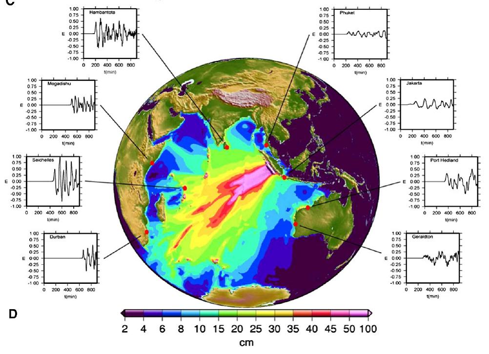
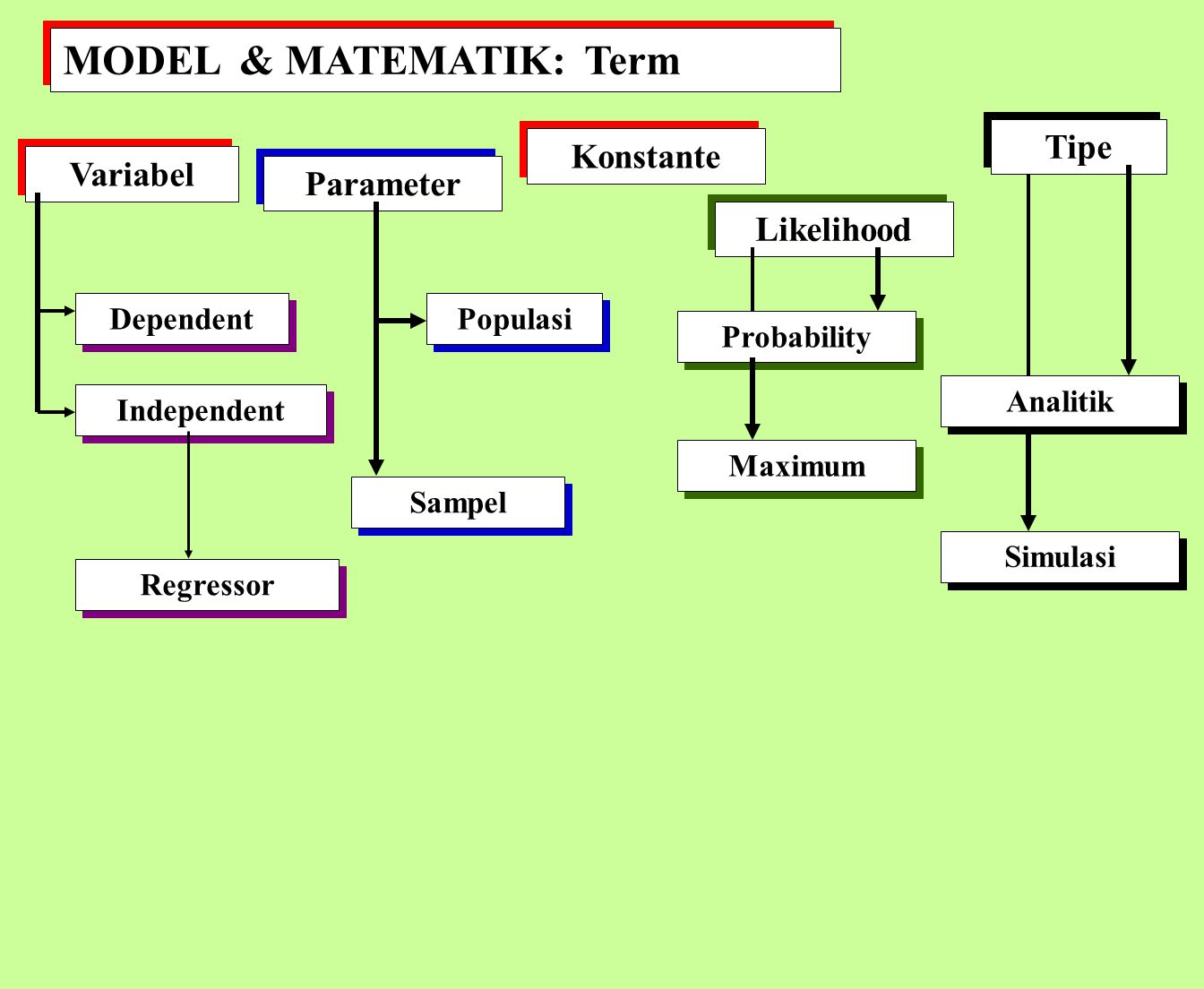


X . IIIIIIIIIIIII Mathematical Model Dynamic Systems
For the analysis and design of control systems, physical systems must
fisisnya model was made.
· Physical model should be able to describe the dynamic characteristics
the system adequately.
· The mathematical model derived from the laws of the physical system
concerned
- The dynamics of the mechanical system is modeled by laws
Newton.
- Dynamics of electrical systems modeled by laws
Kirchoff, Ohm.
· The mathematical model of a system: a set of equations
describes the dynamics of a system adequately.
· The mathematical model can increase accuracy by
model more completely, if necessary
Careful analysis.
· It should be a compromise between the simplicity of the model with accuracy
for analysis output
Simplicity models achieved by considering factors
only important in modeling.
- Modelling with differential equations (not partial),
would eliminate certain nonlinear properties and
Distributed parameters that may exist on
system.
- Modeling a component at low frequencies are not
can be used at high frequencies.
· A system that has the same mathematical model are not always
describe the same physical models (eg analogy system
mechanical with electrical system).
· Two analytical approach:
- Transfer Function (Traditional, for a system SISO)
- State Space (Modern, for modern systems, eg MIMO)
KLASIFIKASI SISTEM
- LINEAR VS NONLINEAR
- TIME-INVARIANT VS TIME-VARYING
- CONTINUOUS-TIME VS DISCRETE-TIME
- DETERMINISTIC VS STOCHASTIC
- LUMPED- VS DISTRIBUTED - PARAMETERS
- TRANSFER FUNCTION VS STATE SPACE
- LINEAR VS NONLINEAR
- TIME-INVARIANT VS TIME-VARYING
- CONTINUOUS-TIME VS DISCRETE-TIME
- DETERMINISTIC VS STOCHASTIC
- LUMPED- VS DISTRIBUTED - PARAMETERS
- TRANSFER FUNCTION VS STATE SPACE
X . IIIIIIIIIIIIII FUNCTION TRANSFER SYSTEM FOR LINEAR
To understand the complicated system, it first gets her mathematical models, which are quantitative. This is because the relationship between system variables and mathematical models of control systems the situation may take the form of dynamic, changeable. The equation is often used differential equations and linear that a solution made it easier by using Laplace transformation. In practice the system is so complicated it would require assumptions about how the system works tersebut.Oleh therefore, required consideration of a physical system by making assumptions (assumptions) and melinierkan the system. Finally, in the completion of utilizing some mathematical tools.
For example: a simple system consisting of a mass of springs and dampers
Linear Approach of Physical Systems
Most systems-linear physical system in which the variable price limit will eventually not be linear if the value of the limit is passed. For example, if the system is linear mass of the spring only for the masses to experience a small deviation y (t), but if y (t) has been constantly increasing, spring will be too stretched and broken. This, linearity problem of constraints (range) use should be taken into account for each system.
A system can be defined as a linear terms of feedback and gain. For electric circuits, as gains are electric currents enter r (t), while the response is
voltage v (t). So the linearity of the system depends on the strengthening of x (t) and the response y (t). If the system to its prior condition corroborated x1 (t) would then provide a response y2 (t), and if the system is linear given amplifier x1 (t) + x2 (t) and the response diterjadi y1 (t) + v2 (t), p this is called the principle of superposition.For a system that is characterized by the relationship y = x2 is not linear because of the nature and properties of superposition of togetherness. The system described by the equation y = mx + b is said to be linear, but the system can be considered linear around the working point x0, y0 for small changes x and y. when x = x0 + x, y = y0 + y we gety = mx + b
To obtain a linear approach using Laplace transformation on the physical system intended to simplify differential equations simplify the settlement of complex issues. Completion of the response time (function of time) obtained at the following stages:
1. Differential Equations;
2. Laplace transform to differential equations;
3. Solving algebraic equations obtained.
A short discussion of the existence of Laplace transforms are often encountered in describing the decline, for example:
f (t) = a function of time t such that f (t) = 0 for t <0;
s = complex variable; integral = operator symbol which indicates that the magnitudes are transformed by Laplace integrals;
F (s) = function of time t such that f (t) = 0 for t <0;
X . IIIIIIIIIIIIIII Simulation and Model
UNDERSTANDING THE SYSTEM AND MODEL
A system is defined as a set or combination of parts that make up a whole complex. But not all of the bodies and groups can be called a part of a system that did not qualify their unity (unity), functional relationships, and any useful purpose. An area with a variety of resources and activities in it is a complex system. In the spatial planning of an area clearly the three conditions can be met, which are land-based spatial planning is a unity in which there is a functional relationship between sectors or part in achieving the goal of optimizing the utilization of spatial region. The functional relationship is reflected in the relationship between the social, economic, and biophysical region. These three conditions will interact with the functions that can be explained. Social conditions, for example, changes in demographic situation will affect economic activity which in turn affects the use of the space that will transform the region biophysical conditions. The model is defined as a representation or abstraction of an object or situation.
System: A collection of elements that work together to achieve the expected goals. The system can also refer to a collection of objects that interact with each other and work together to achieve a logical goal in a complex environment. Objects that are components of the system may be the smallest objects and can also be sub-systems or smaller systems again. In this definition included elements of the environment because the system environment provides a very important role on the behavior of the system. How the system components interact, it is in order to anticipate the environmental Viewing system not only defines the technical components of the system, but more than that it must also know the behavior and the variables that exist in it. At least an analysis of the system should be able to make the conception of the system. There are several ways to be able to design, analyze and operate a system. One way is to do modeling, create a model of the system.
Model is a very useful tool for analyzing and designing systems. As a highly efficient communication tool, the model can show how an operation works and is able to stimulate to think how to improve or fix it. The model is defined as a logical description of how the system works or the components interact. By creating a model of a system it is expected to be easier to perform the analysis. It is the modeling principle, namely that the modeling aims to simplify the analysis and development. Modeling is a way to learn the system and the model itself and also an assortment of perilakunya.Model difference: an overview of a system, can be physically or mathematically.
Relationships: to know the behavior of the real system is complex, made models. In a dynamic system, this model can be realized in computer programming is called simulation.
Simulation is a technique to mimic the operations or processes that occur in a system with the aid of computer equipment and based on certain assumptions that the system can be studied scientifically (Law and Kelton, 1991). In the used computer simulations to study the numerical system, where data collection to estimate the statistics to obtain the original characteristics of the system. Simulation is a good tool to use, especially if it is required to perform experiments in order to find the best comments of the components of the system. This is because it is very expensive and take a long time if the experiment is tried in real terms. By doing simulation studies it can be determined in a short time the right decision and at a cost that is not too big because everything is done by computer. Simulation approach begins with the development model of the real system. The model should be able to show how the various components in the system interact to completely describe the behavior of the system. Once the model is created then the model is transformed into a computer program that allows it to be simulated. Or simulation can also be defined as a clone of a dynamic system using computer models used to evaluate and improve system performance.
Simulation: the process of designing a mathematical model or logic of the system further experiment with the model they will be to describe, explain and predict the behavior of the system
- The advantages of a simulation as follows:
v Allows details to be included
v It can compare the design of other systems
v Can control the timescale
v existing system is not required
v Most real systems with stochastic elements can not be described accurately by a mathematical model that evaluated analytically. Thus simulation is often the only way.
v Simulation allows estimation of the performance of the existing system with several different operating conditions.
v The draft-draft recommended alternative system can be compared via simulation to get the best.
v In the simulation can be maintained better control of the experimental conditions.
v The simulation allows the study of the system with a long time frame in a shorter period of time, or learn how detailed work in extended time.
- Whereas the weakness of a simulation as follows:
v It is difficult to generalize the results
v It is difficult to consider all cases values / parameters
v It is difficult to determine the sensitivity
v The time to develop and execute simulation
v Attempts to validate the model and analyze the output data
v Each step stochastic simulation model experiments only produce estimates of the characteristics of the actual system for certain input parameters. Analytical model is more valid.
v The simulation model is often costly and take a long time to develop.
v Output of large amounts resulting from the simulation is usually looked convincing, though not necessarily the model is valid.
Modeling
and simulation systems evolving so rapidly and has widespread
application in various fields of natural science fields such as physics,
chemistry, biology, medicine to social sciences such as economics,
social and political. In
college alone simulation techniques have been taught to subjects:
Aeronautics and Astronautik, Electrical Engineering and Computer
Science, Technology and Health Sciences, Mechanical Engineering, Nuclear
Science and Engineering. In Indonesia, material modeling and simulation are given in the study
program Informatics Engineering, Electrical Engineering, Industrial
Engineering, Mechanical Engineering, Engineering Physics, Statistics and
others - others.
As a prerequisite for understanding the modeling and simulation, it is advisable to understand the calculus of differential equations, Laplace transforms, Z transformation, programming languages C / C ++. Implementation of the simulation can use the programming languages C / C ++ and not on application software packages such as MATLAB / SIMULINK only use (use only), as well as C and C ++ and OpenGL support in principle open source (open source), further study can even develop own research algorithms and procedures that exist in the implementation of modeling and simulation.
Sample simulation:
• Simulation of Flying
• Simulation of the macroeconomic system
• Simulation of the banking system
• Simulation of bank service queue
• Simulation game marketing strategy
• Simulation war
• Simulation of car
• Simulation of urban planning
• Simulation of traffic lights
Stages Simulation:
1. Understanding the system to be simulated
2. Develop a mathematical model of the system
3. To develop mathematical models for simulation
4. Make prgram (software) computer
5. Testing, verify, and validate the computer output
6. Execute a simulation program for the purpose tertentuMETODE SIMULATION
MONTE CARLO
Discrete-event
Next-Event Time Advance
Fixed-Increment Time Advance
Taxonomy MODEL
MONTE CARLO vs D-E
Monte Carlo Simulation Model:
stochastic
Static
Discrete-Event Simulation Model:
stochastic
Dynamic
Discrete-Event
Simulations with a computer:
models evaluated numerically, and collected data to estimate the actual characteristics of the model. Examples of application areas of simulation:
The design and manufacturing system analysis.
Evaluate hardware and software requirements for the computer system.
Evaluation of weapons systems or new military tactics.
Communication system design and message protocol.
The design and operation of transport facilities, ie. highways, airports, railways or ports.
Evaluation of the design of the service organization, ie. hospital, post office, or a fast food restaurant.
observing the system not only defines the technical components of the system, but more than that it must also know the behavior and the variables that exist in it. At least an analysis of the system should be able to make the conception of the system. There are several ways to be able to design, analyze and operate a system. One way is to do modeling, create a model of the system. Model is a very useful tool for analyzing and designing systems. As a highly efficient communication tool, the model can show how an operation works and is able to stimulate to think how to improve or fix it. The model is defined as a logical description of how the system works or the components interact. By creating a model of a system it is expected to be easier to perform the analysis. It is the modeling principle, namely that the modeling aims to simplify the analysis and development. Modeling is a way to learn the system and the model itself and also a variety of differences in behavior.
Experiment with the actual system vs. experimental model system.
If a system is physically possible and thus costly to operate in accordance with the conditions (scenario) that we want it this way is the best way for the results of these experiments are completely in accordance with the system being studied. However, such systems rarely exist and shutdown of the system for the purposes of the experiment will take a huge cost. In addition to a system that does not exist or systems are still in the design of the experiment with the actual system obviously can not be done so the only way is to use the model as a representation of the actual system.
v Physical Model Mathematical Model vs.
Physical models take on most of the physical properties of the things they represent, so as to resemble the actual system but in a different scale. Although rarely used, this model is useful in systems engineering. In the study, a mathematical model is used more often when compared to the physical model. In the mathematical model, the system is represented as logical relationships and quantitative relationship to then manipulated so that it can be seen how the system reacts.
v Solutions Analytical vs. Simulation.
After successfully formulated a mathematical model, the model learned back whether the model that has been developed to address questions related to the purpose of studying the system. If the model established quite simple, then the mathematical relationships can be used to find an analytical solution. If the analytical solutions can be obtained fairly easily and efficiently, then you should diigunakan analytical solutions because this method is able to provide optimal solutions to problems faced. 4
v Classification Model Simulation.
Basically, the simulation models are grouped in three dimensions [Law and Kelton, 1991]:
@) Static Simulation Model with Dynamic Simulation Model.
Static simulation model is used to represent the system at a given time or a system that is not affected by the time change. While the dynamic simulation models are used if the system being studied is affected by the time change.
@) Deterministic Simulation Model with Stochastic Simulation Model.
If the simulation model to be formed does not contain a random variable, then the simulation model is said to be as a deterministic simulation. In general, the system being modeled in the simulation contains several inputs that are random, then in such a system simulation model constructed called stochastic simulation model.
@) Continuous simulation models with Discrete Simulation Model.
To classify a simulation model whether discrete or continuous, is determined by the system being studied. A system is said to be discrete if the variable system that reflects the status of the system is changed at a certain point in time, while the system is said to be continuous if the system variable changes take place on an ongoing basis in line with changing times.
- Studying the system by simulating:
numerically run the model for giving input and see its effect on output.
Features simulation software required:
Generating random numbers from a probability distribution U (0,1).
Generating random values of certain probability distribution, ie. exponential.
Advancing simulation time.
Determining the next event from the event list and gives control to block the correct code.
Add or delete a record on the list.
Collect and analyze data.
X . IIIIIIIIIIIIIIII Neural network for model mathematic dynamic
Neural Network formally defined as "generalization of mathematical models of biological neural systems". Artificial Neural Network (ANN) has been widely used for a variety of applications such as character or voice recognition, image processing, stock price prediction, prediction of currency exchange rates, and so forth. In general applications- the application requires processing in real time (real time).
Artificial Neural Network (ANN) than can be implemented with software, also with hardware. The hardware has advantages over the software on the speed. Operations performed faster hardware than software. Therefore, hardware neural network can be used to serve real-time visualization applications. Neural Network consists of several processing units that perform accumulation (summation) of the input weighted inputs and produces an output with a particular activation function. The properties of the network is determined by the topology of the network, the interconnection weights and activation functions. As a model, the Neural Network has the following capabilities: The ability to model the transmission of signals between neurons imitation through in one direction, called the connection. Each input connection is only connected to one other clone neuron output connections. Each output connections can be associated with some other clone neuron input connections. The ability to model the weighting of each connection. In most types of neural networks, the connection weight value will be multiplied with the transmission of signals. The ability to model neuron activation function on each clone to determine the output signal. The ability to model the structure of distributed information. That is, processing information is distributed on multiple neurons at the same clone. Each neuron clone must have local memory and capable of doing pengolahaninformasi locally. Modeling Neuron-Pits McCulloch, in 1943 made five basic assumptions about the biological nervous system, namely: Activities of neurons are all-ornone. To make neurons emit a signal (active) required number of synapses that excites neurons in a certain period. A number of neuron's synapses could inhibit active (inhibitory). The existence of delay in the nervous system caused by synapses delay. Network interconnection structure does not change over time. Based on this assumption, the McCulloch-Pitts neuron model building imitations that mimic the workings of biological neurons.
 Neuron Model
 The model neuron has n input signals, namely x1, x2, ..., xn with x ε {0,1}. Each signal is then modified by the weight of synapses w1, w2, ..., wn so that the incoming signal to the neuron is xi1 = xi wi, i = 1,2, ..., n. Furthermore, neurons will calculate the sum of the entire input signal which has been modified: net = x_ {1} W_ {1} + x_ {2} W_ {2} + ... + x_ {n} {n} W_ net = \ sum_ { i = 1} ^ {n} x_ {i} W_ {i} activation functions contained in a mock neurons generally a non-linear function. This activation function that determines whether neurons will undergo activation or not. Activation level embodied in a threshold value (threshold). Activation function that is normally used is the step function (step function), the function of the slope (slope function), and the sigmoid function. In the model of McCulloch-Pitts, activation function is a step function so that: f (net) = \ left \ {_ {0, jikanet <\ theta} ^ {1, if net \ geq \ theta} where θ = a threshold value
The Basic Model of Neural Network Friday, November 6th, 2015. | Theory Electronics Mesothelioma Law Firm, Sell Annuity Payment Adopting the basic essence of the nervous system biology, neural described as follows: Receiving input or input (either from the data entered or from the output of nerve cells in the neural network. Each input comes via a connection or relationship which has a weight (weight). Each nerve cell has a threshold value. Total weight of inputs and reduced the threshold value will then get an activation of the nerve cells (post synaptic potential, PSP, of the nerve cells). Signal activation then becomes a function activation / transfer function to produce an output of nerve cells.
If stage activation function used (output of nerve cells = 0 if the input <0 and 1 if input> = 0) then the action of nerve cells together with nerve cell biology described above (the reduction of the threshold value of the amount of weight and compare with 0 is equal to compare a weighted sum of the threshold value). Usually stages rarely used functions dalan Neural Network. Activation function can be seen in the following figure. Image Activation Function Neural Network
Image Activation Function Neural Network
 |
|||||||
| How nerve cells interconnected? If a tissue to be used for various purposes then it should have an input (will bring the value of a variable from the outside) and output (of prediction or control signal). Input and output in accordance with the sensor and motor neurons as the signal coming from the eye and then forwarded to the hand, In this case there are nerve cells or neurons in the hidden layer plays a role in this network. Input, hidden and output layers of nerve cells is required to connect to each other. |
Mathematical models can be classified in various ways, and its use is called simulation. Electronic spreadsheet (spreadsheet) is a good tool to create mathematical models. This worksheet can be used for both static and dynamic models and make managers can play a game of "what if" (what-if-game).
Artificial intelligence can be one component of DSS. By adding the knowledge base and the inference engine, DSS can suggest solutions to problems to the manager.
If groupware is added to the DSS, the DSS will be a group decision support systems (group decision support system-GDSs). GDSs can be placed in several different places so it is conducive to problem solving group.
The troubleshooting process consists of four basic elements, namely:
I) standard,
I) standard,
II) information,
III) restrictions, and
IIII) an alternative solution.
Problem Solving and Decision Making
SIM is a system that provides information for use in decision making in order to resolve the problem for users.
Solving problems (problem solving) consists of a response to things going well, and the things that went badly by defining the problem (problem) as a condition or event that is dangerous or could endanger the company, or useful, or could benefit. In the process of solving problems seen managers in decision-making (decision making), which is a matter of choosing among alternative solutions to problems. The decision (decision) is defined as the act of choice and often need to take many decisions in the process of solving one problem only.
Phase Troubleshooting
According to Simon, the problem solver engaged in:
· Intelligence Activities. Looking around the environmental conditions that must be solved.
· Activities design. Discovering, developing, and analyzing the actions that may be performed.
· Activities elections. Selecting a particular course of several available.
· Activity Assessment. Check out the options and then
Approach and Importance of Perspective System
The systems approach is a series of steps which are grouped into three stages of preparedness, efforts to defining and solving efforts.
In using a model system of public and environmental model as the basis for solving problems, perspectives systems (systems view) that sees the business operating as a system that is part of the wider environment. This is an abstract way of thinking, but it has a potential value to managers. How to view the system would:
@. Prevent the manager to avoid confusion due to the complexity of the organizational structure and detail work.
@. Stresses the importance of having a good purpose.
@. Stresses the importance of all parts of the organization to work together.
@. Remove the relationship between the organization and its environment.
@. Placing a high value on information obtained from the input that can only be achieved through a closed circulatory system.
Build Concepts and Problem Solving Process Elements
Most of the problems were solved managers can be regarded as problems of the system. For example, the company as a system does not function properly. Alternatively, there are problems with the inventory system, sales commission system, and so on. System problem solution is the solution that makes the system meets its objectives by the most excellent, as reflected in the standard of performance of the system. This standard describes the desired situation (desired state) what should be achieved the system. In addition, the manager must have information that describes the current state (current state) the achievements of the current system. If these two circumstances are different, then there is a problem is the cause and must be solved.
The difference between the current state to the desired state called criteria solution (solution criterion), or what should happen for the current situation turns into a desirable situation. Of course, if the current situation shows a higher level of performance compared to the desired state, then the task that must be done is not to equate the current situation. Rather, the task that must be done is to keep the current situation remain at a higher level. If the high level of performance can be maintained, then the desired situation should be improved.
The responsibility of the manager is to identify alternative solutions, which is always there. This is one step of the problem solving process in which the computer is not too much help. Managers typically rely on their own experience or seek assistance from noncomputer information processing, such as input from other parties both inside and outside the company.
After various alternatives are identified, information systems can be used to evaluate it. This evaluation must consider the constraints (constraints) which exist, which can be derived both from internal and environment. Internal restrictions (internal constraint) usually in the form of limited resources that exist in the company. For example, the IT unit can not design a CRM system because of a lack of expertise in OLAP. Environmental restrictions (environmental constraints) in the form of pressure from various environmental elements that limit the flow of resources from and out of the company. One example is the increase in interest rates by the Federal Reserve Board which increases the cost of the expansion of the plant.
@ Choosing the Best Solution
Selection of the best solution can be achieved in many ways. Herry Mintzberg, a management theorist, has identified three approaches:
· Analysis
Evaluation of options systematically, taking into account the consequences of those choices on the organization's objectives.
One example is the judgment made by the members of the supervisory committee SIM to decide which approach should be taken in implementing executive information systems.
· Assessment
Thought processes are carried out by a manager. For example, production managers apply the experience and intuition in evaluating the proposed new plant images from mathematical models.
· Offers
Negotiations between several managers. One example is a process of give and take that took place between the members of the executive committee of the market which should be entered next. Here is the place where political influence in the enterprise can be clearly seen.
@ Problems versus Symptoms
It is important for us to understand the difference between a problem and a symptom of a problem. Otherwise, we can spend a lot of time and money to resolve problems that wrong or something that is not actually a problem. Symptoms (symptom) is a condition that produced the problem. Often a manager look at the symptoms and not the problem.
Structural Problems
The mathematical model called formula EOQ (economic order quantity) can tell how the problem should be resolved. Problems like this are called structured problems (structured problem)
because it consists of elements and the relationships between the
various elements of which were understood by the problem solver.
Unstructured problems (unstructured problem) is a problem that does not have the elements or relationships between elements that are understood by the problem solver. One example of an unstructured problem is deciding which movie that we like. Business managers often do not have enough tools to define problems like this in a structured way.
Actually, just a bit of a problem in an organization that is really structured or completely unstructured. Most problems are issues where the manager has a less than perfect understanding of the various elements and the relationships among them. Semistructured problems (semistructured problem) is a problem that consists of several elements or relationships that are understood by the problem solver and some that can not be understood. One example is the choice of location to build a new factory.
Some elements, such as land prices, taxes, and fees for sending raw materials, can be measured with a high degree of accuracy. But other elements, such as the danger of the environment and the behavior of people around, it is difficult to be identified and measured.
After the prescribed procedures, the computer can solve problems that structured without manager involvement. However, managers often have to do all the work to solve unstructured problems. In semistructured problem areas were spacious, the manager and the computer can work together to find solutions.
Type Decision
In addition to providing the stages of problem solving, Herbert A.Simon also found a method to classify the decision, namely:
· Decision programmed (programmed decision) is "repetitive and routine, in the case of certain procedures used to treat it, the decision does not need to be considered de novo (new) every time they happen."
· Decisions are not programmed (nonprogrammed decision) are "new, unstructured, and full of consequences. There is no reliable method to handle this kind of problem because the problem has never arisen before, or because of the nature and difficult to explain and complex structure, or because the problem is so important that it requires special handling. "
Decision Support Systems
The term structured decision systems (structured decision-SDS system) is used to describe systems that are able to resolve the identified problems. The issues under difficult line of computer processing, and Gorry and Scott-Morton used the term decision support systems (decision support system DSS) to describe a system that can provide the necessary support.
Since 1971, DSS has become the type of information system is now the most successful and computer applications for troubleshooting the most productive.
Since 1971, DSS has become the type of information system is now the most successful and computer applications for troubleshooting the most productive.
Model DSS
When DSS is designed for the first time, this model produces special and periodic reports as well as the output of a mathematical model. This special report contains a response to a request to the database. After DSS implemented, capability that allows the troubleshooter to cooperate in a group is added to the model. Extra groupware software allows the system to function as a decision support system group (group decision support system-GDSs). Most recently, artificial intelligence capabilities have also been added along with the ability to engage in OLAP.
When DSS is designed for the first time, this model produces special and periodic reports as well as the output of a mathematical model. This special report contains a response to a request to the database. After DSS implemented, capability that allows the troubleshooter to cooperate in a group is added to the model. Extra groupware software allows the system to function as a decision support system group (group decision support system-GDSs). Most recently, artificial intelligence capabilities have also been added along with the ability to engage in OLAP.
Mathematical Modelling
The model is an abstraction of something. The model represents an object or activity, the so-called entity (entity). Managers use models to represent problems that must be solved. Object or activity that is causing the problem referred to by the entity.
The model is an abstraction of something. The model represents an object or activity, the so-called entity (entity). Managers use models to represent problems that must be solved. Object or activity that is causing the problem referred to by the entity.
Type Model
There are four basic models, namely:
@. Physical Model (Physical model)
A three-dimensional representation entities. Physical models used in the business world include a scale model for shopping centers and prototypes of new cars.
The physical model is made to achieve the goals can not be met by a real object. For example, the physical model allows designers to evaluate the design of objects, such as airplanes, and make changes before actual construction. This will save time and money.
@. Model Narrative
One type of model used by the manager every day is a model of narrative (narrative model) that describes the entities with words spoken or written. The listener or reader can understand the entity of the narrative. All business communication is a model of narrative, thus making the narrative models of the most popular types of models.
@. Model Graphics
Another type of model continues to be used is a graphical model. Model graphic (graphic models) describe the entity with the abstraction of lines, symbols, or shapes. Total economic order (economic order quantity-EOQ) is the optimum amount of addition of the stock to be ordered from the supplier. EOQ balancing the cost of purchasing the stock and the cost to store it until the stock is used or sold.
Graphical model is also used in the design of information systems. Most devices that are used by system developers graphic nature. Entity relationship diagrams, class diagrams and data flow diagrams are some examples.
Mathematical Model
Any formula or mathematical equation is a mathematical model (mathematical model). Most mathematical models used business managers as complex as that used to calculate the EOQ.
Storage costs include all costs incurred in the storage of goods, such as insurance, damage and loss due to theft.
Some mathematical models use hundreds or even thousands of equations. For example, a financial planning model designed Sun Oil Company in the first years of his license usage using about 2,000 equations. Large model like this tend to be slow and difficult to use. The ongoing trend today is the use of a smaller model.
Usage Model
All four types of models provide insight and facilitate communication. In addition, a mathematical model has predictive ability.
@) Provide understanding.
The model is typically simpler than its entity. Entities are objects or processes. Entities can be more easily understood if the various elements and relationships contained therein shown more modest. After a simple model can be understood, the model gradually be made more complex so that it can represent a more complex entity. However, the model can only represent entities. The model can not really act like real entity.
@) Facilitate Communications
All four types of models can communicate information accurately and quickly to the people who understand the meaning of shapes, words, graphics, and mathematical.
@) Predicting the future
The precision indicated mathematical model to represent the capabilities that are not available on other models. The mathematical model can predict what will happen in the future, but is not 100 percent accurate. No model is as good as it was. Because assumptions usually must be made based on the amount of data
entered into the model, managers must use judgment and intuition in
evaluating the output.
Mathematical Model
The mathematical model can be classified into three dimensions: the influence of time, the level of confidence, and the ability to achieve optimization.
@) Static or Dynamic Model
Static Model (static model) does not involve the time as one of the variables. This model with regard to the situation at a particular time. In other words, the circumstances are such footage. Model that includes time as a variable called dynamic model (dynamic model). This model describes the behavior of an entity over time, such as moving images or movies.
@) Probability or Deterministic Model
Another way to classify a variety of models based on whether a formula involving the probability or not. Probability (Probability) is a chance that something will happen. The probability ranged from 0.00 (for something that has no chance of happening) to 1.00 (for something that is inevitable). Models involving probabilities is called the probability model (probability model). If not, then the model is a deterministic model (deterministic model).
@) Optimization Model or suboptimization
Model optimization (optimizing model) is a model that select the best solution from various alternatives are displayed. So that a model can do this, the problem should be structured very well.
Model suboptimization (suboptimizing model) is often called a model satisfying (satisficing model) allows a manager to enter a set of decisions. Once these steps are completed, the model will project results.
simulations
The act of using a model called the simulation (simulation). Simulation occurs in certain scenarios and predict the impact of those decisions that solves the problem.
Scenario term scenarios (scenario) is used to describe conditions that affect the simulation. Data elements that define this scenario is called scenario data elements (scenario of data element). This model can be designed such that the variable-shaped scenario data elements, enabling determination of different values.
Variable Decision and Engineering Simulation
The input values are entered managers to measure the impact on the entity called the decision variables (decision variables).
The manager usually performs optimization models only once. This model produces the best solution using specific scenarios and decision variables. However, it is also important to run the model suboptimization repeatedly, in order to find the combination of decision variables that yield satisfactory results. Looping process to try a variety of alternative decisions how the game is called if (what-if game).
Each time the model is run, only one of many variables that decision should be changed so that its effects can be seen. In this way, the troubleshooter can systematically find the combination of decisions that will produce solutions to problems.
Example of Modeling
Corporate executives can use mathematical models to make some key decisions. These executives can simulate the impact of:
· Product Price.
· Total plant investment required to provide the capacity to manufacture the product.
· The amount to be invested in marketing activities, such as advertising and direct sales.
· The amount to be invested in research and development.
In addition, the executives want to simulate four quarters of activity and produced two reports:
@. The operational reports that include non-monetary values such as the potential market (demand) and factory capacity as well,
@. The income statement that reflects the results monoter.
Strengths and weaknesses of modeling
The manager who uses mathematical models can benefit through the following:
· Process modeling can be a learning experience. The manager will always learn something new about the actual system through any modeling project.
· Speed simulation process allows a large number of alternatives could be considered by providing the ability to evaluate the impact of decisions in a short time. In just a few minutes, we can simulate several months, quarterly, or annual operations.
· As previously discussed, the model provides prediction capabilities view to the future that can not be provided by methods other information providers.
· The model is not as expensive as a trial effort. Process modeling is expensive when viewed from the time and cost of designing hardware and software needed to perform simulations, but these costs are not as high as the costs incurred if a bad decision is implemented in the real world.
Advantages of this modeling can be reduced because two basic flaws:
· Difficulty to model business system will produce a model that does not include all influence over the entity. For example, in the model just described, someone at the company must estimate the value of the data elements scenarios. In addition, the mathematical formulas usually only a forecast on the behavior of the entity. This means that subjective judgments are large enough to be applied in implementing the decisions made based on simulation results.
· The ability of high-level mathematical models needed to design more complex. Moreover, this kind of capability is also needed to interpret the outputs properly.
Modelling Using Electronic Spreadsheet
A breakthrough technology that enables the problem solver to construct a mathematical model and not simply rely on an information specialist or a management scientist is an electronic spreadsheet. Prior to the worksheet (spreadsheet), a mathematical model programmed in technical language such as Fortran or API, which is outside the competence of problem solvers who do not have a computer background. When the spreadsheet is present, it seems clear that this technology will be a good tool to create mathematical models.
A breakthrough technology that enables the problem solver to construct a mathematical model and not simply rely on an information specialist or a management scientist is an electronic spreadsheet. Prior to the worksheet (spreadsheet), a mathematical model programmed in technical language such as Fortran or API, which is outside the competence of problem solvers who do not have a computer background. When the spreadsheet is present, it seems clear that this technology will be a good tool to create mathematical models.
@. Static Modeling Capability
Rows and columns of an electronic spreadsheet makes it ideal for use in a static model.
@. Dynamic Modeling Capability
Worksheets are very suitable to be used as a dynamic model. The columns are available very appropriate for the time period.
Rows and columns of an electronic spreadsheet makes it ideal for use in a static model.
@. Dynamic Modeling Capability
Worksheets are very suitable to be used as a dynamic model. The columns are available very appropriate for the time period.
Playing the game "What If"
The worksheet is also useful to play the game of "what if", where fixers manipulating one or more variables to see the impact of the simulation results.
Interface Model Worksheet
When using the worksheet as a mathematical model, the user can enter data or make changes directly to the cells of a spreadsheet or can use a graphical user interface.
Artificial Intelligence
DSS emphasizes the use of mathematical modeling and the submission of requests to the database. Not long after, the designers of DSS began to realize the need to incorporate artificial intelligence. Artificial intelligence (artificial intelligence-AI) is the activity of providing such machines as computers with the ability to display behavior that would be regarded as intelligent as if the ability displayed by humans. AI is the most advanced computer applications because the application is trying to imitate the way the human mind.
DSS emphasizes the use of mathematical modeling and the submission of requests to the database. Not long after, the designers of DSS began to realize the need to incorporate artificial intelligence. Artificial intelligence (artificial intelligence-AI) is the activity of providing such machines as computers with the ability to display behavior that would be regarded as intelligent as if the ability displayed by humans. AI is the most advanced computer applications because the application is trying to imitate the way the human mind.
History of AI
Seed AI was first deployed just two years after General Electri applying the first computer used for business use. 1956, and the term artificial intelligence was first made by John McCarthy as the theme of a conference held at Dartmouth College. In the same year, the first AI computer program called Logic Theorist, announced. Logic Theorist limited ability to think (proving theorems calculus) to encourage scientists to design another program called General Problem Solver (GPS), which is intended to be used in solving all kinds of problems. This project turned out to make the scientists who first compiled the program overwhelmed and defeated by the AI research computer applications that are not too ambitious as MIS and DSS. But over time, continuous research finally paid off, and AI has been a solid computer application area.
AI Territory
AI applied in the business world in the form of expert systems, neural networks, genetic algorithms, and intelligent agents.
@. Expert System
Expert systems are computer programs that seek to represent the knowledge of human expertise in the form of heuristics. The term heuristics comes from the Greek word eureka, which means "find." Heuristic (heuristic) is a rule that a standard or rule to guess well.
Heuristic algorithms do not guarantee the best results usually obtained in mathematical models, but heuristic usually offer results that is specific enough that it can be useful. Heuristics allows the expert system to function in such a way that konsistem with human expertise, and advises users how to solve the problem. Because the expert system serves as a consultant, the act of using this application is called consultation (consultation) since the user consults the expert system for advice.
Expert systems are designed by specialists of information (often referred to engineer knowledge (knowledge engineer)) who have specific expertise in the field of artificial intelligence. The knowledge engineer is very skilled in getting knowledge from an expert.
@. An artificial neural network
Artificial neural networks (neural networks) mimics the physiology of the human brain. These networks are able to find and distinguish the pattern, making it very useful in business in the area of speech recognition and optical character recognition.
@. Genetic Algorithms
Genetic algorithms (genetic algorithms) develops the "strongest survivors" to allow problem solvers to produce solutions to problems is getting better. For example, investment bankers can use to choose the best investment portfolio for its clients.
@. Intelligent Agents
Intelligent agents (intelligent agents) used to perform tasks related to computer repeatedly. One example is data mining, knowledge discovery which allows a data warehouse system to identify the relationship data that was previously unknown.
* Attractiveness Expert System
The expert system offers unique capabilities as decision support systems, namely:
@. The expert system provides the opportunity to make decisions that exceed the ability of a manager. For instance, a new investment in the bank employee can use an expert system designed by a financial expert and, thus, combining the expert knowledge into their investment decisions.
@. Expert systems can explain the reason to go to a decision. Often, the explanation of how the solution was reached more valuable than the solution itself.
* Configuration Expert System
An expert system consists of four main parts: the user interface, knowledge base, interface engine, and engine development.
· User Interface
The user interface allows managers to enter instructions and information into the expert system and receive information from the system. These instructions define the parameters to direct the expert system in its thought process. Input-shaped information value that is associated with a particular variable.
The expert system is designed to recommend a solution. These solutions are then provided with an explanation. There are two types of explanations: Explanation of the question given the manager and an explanation of the problem solution.
· Knowledge Base
The knowledge base (knowledge base) contains facts that describe the problem as well as knowledge of imaging techniques that explain how the facts logically touch. Domain term problems (domain) is used to describe the problem areas.
One technique to describe the popular knowledge is the use of rules. Rule (rule) to determine what to do in a given situation and consists of two parts: a condition that can be right or wrong and what to do if the condition is true. Example rules are:
If Indeks.Ekonomi> 1.20 and Indeks.Musiman> 1.30 Then Prakiraan.Penjualan = 'EXCELLENT'
All the existing rules in an expert system called the set of rules (rule set). The number of rules in the rule sets can vary from about a dozen rules for an expert system is simple to 10,000 complicated rules to set.
· Inference Engine
Inference engine (inference engine) is part of the expert system that do the thinking by using the contents of the knowledge base in a particular order. During the consultation, the inference engine checking rules knowledge base one by one, and if the requirements of the rule is true, then the action will be implemented. In the terminology of expert systems, the rules laid off if any action is taken.
Regulatory examination process continues until one by one the whole set of rules has been passed. More than one inspection is usually required to give a value to the solution of problems, called the variable of interest (goal variable). Examination continues to allow it to lay off some of the rules. When there are no more rules can be dismissed, the thought process can be stopped.
· Engineering Development
The fourth major component of the expert system is the engine of development, which is used to make the expert system. There are two basic approaches are available: the programming language and framework of expert systems.
Framework of expert systems (expert systems shell) processor is ready to use and can be customized for a particular problem by adding an appropriate knowledge base. Now, most of the interest to implement the expert system to business problems involving the use of templates.
One example of the problem domain that uses the framework of expert system is a computer customer assistance. When a customer support expert systems are used, the user or customer support staff members to communicate directly with the system, and the system then try to resolve the problem.
Expert systems help customers use a variety of imaging techniques knowledge. One popular approach is called the thinking-based cases (case-base reasoning CBR). This approach uses historical data as a basis to identify problems and recommend solutions.
Expert system framework has made affordable artificial intelligence companies that do not have sufficient resources to design their own systems using a programming language. In the business area, the framework of an expert system is the most popular way for many companies to implement a knowledge-based system.
@. Decision Support Systems Group
Various committees, project teams, and task forces that exist in many companies is an example of a team approach to problem solving. Recognizing this fact, the developers have adapted DSS system into the problem solving group.
* The concept of GDSs
Decision support systems group (group decision support system-GDSs) are "computer-based system that helps a group of people perform a task (or achieve) the same and provides an interface for shared use." Glossary of other terms are also used to describe the application of information technology into a group situation. This term include support system groups (group support system-GSS), cooperation aided computer (computer-supported cooperative work-CSCW), support collaborative work computerized (computerized collaborative work support), and electronic meeting system (electronic meeting system-EMS ). The software used in these situations is named groupware.
* How GDSs Help Troubleshooting
The assumption underlying the GDSs is better communication to the creation of a better decision. Better communication is achieved by keeping the group discussion focused on the issue being discussed, so time is not wasted. Extra time owned can be used to discuss the issues in more detail, so we get a better definition of the problem. Alternatively, the extra time you have can be used to identify alternatives that previously seemed impossible. Evaluation of alternatives that more would increase the chances of getting a better solution.
* Location of Environmental GDSs
GDSs help solving the problem by providing a conducive location for communication. At each location, the group members can meet at the same time or at different times. If the members met at the same time, then this location is called synchronous exchange (synchronous exchange). One example is the meeting of the committee. If the members meet at different times, then this location is called an exchange asynchronous (asynchronous exchange). One example is reciprocated mutual communication via e-mail.
* Space Decision
Lounge decision (decision room) is a small group of people who meet in person. This room helps communication through a combination of furniture, equipment and premises. Equipment includes a combination of a computer, microphone recorder, video camera, and the big screen. In the middle of the room lies a facilitator console. The facilitator (Facilitator) is someone whose primary job is to keep the discussion on track.
Based on the specified settings for each session, a message is entered by a member of the group to another member can be displayed on a wide screen for viewing the entire group. Other materials that are important to this discussion can also be displayed on the media such as PowerPoint pictures, videotapes, color slides and transparencies.
Two unique features of GDSS is a parallel communications and anonymity. Parallel communication (parallel communication) occurs when all participants post a comment at the same time, and anonymity (anonimity) is when no one can find out who is giving particular comment. Anonymity allows the participants to say what they think without fear of being ridiculed by the other group members. In addition, this feature allows each idea to be evaluated based on the strengths and not on who gave them.
* Network Local Regions Decision
If it is impossible for a small group of people to meet in person, then the members can interact via the LAN. A member can enter comments into the computer and see the comments of the other members on the screen.
* Legislative Session
If the group was too large for a chamber decision, it will be necessary legislative session. The large size will restrict communication. Participation opportunities evenly by all members of the group to be reduced or the time available will be reduced. One solution to this problem is the facilitator decide which material should be shown on the screen to see the whole group.
* The Conference of Computer Mediated
Some virtual application allows communication between large groups that have members scattered in different geographical areas. These applications are collectively known as remote conferencing applications, which include computer conferencing, audio conferencing and video conferencing.
* Putting in Place
It has been seen how the decision support coverage provided by DSS has widened compared to when Gorry and Scott-Morton was first expressed an idea to solve semistructured problems. The expansion of this scope is a witness to the success of DSS. This concept has worked very well so that developers continue to think of new features to be added.
When artificial intelligence is added, this feature actually change the character of DSS. Someone once described the difference between the DSS and expert systems by way of explaining that when a manager uses DSS, then he sat in front of computer and trying to discover how to use the information display to solve the problem. When managers use expert system, the manager sitting at the computer, but a consultant sitting next to the manager and advise on how to solve the problem. Artificial intelligence allows DSS to provide decision support levels previously not imagined by the visionary DSS.


