


PID controller miracle, bringing the output of the system temperature, speed, light - to the desired set point can adjust quickly and accurately. Although there are a number of ways to do this, the circuit under separate three terms in the three op amp individuals.
X . I Tuning PID Control.
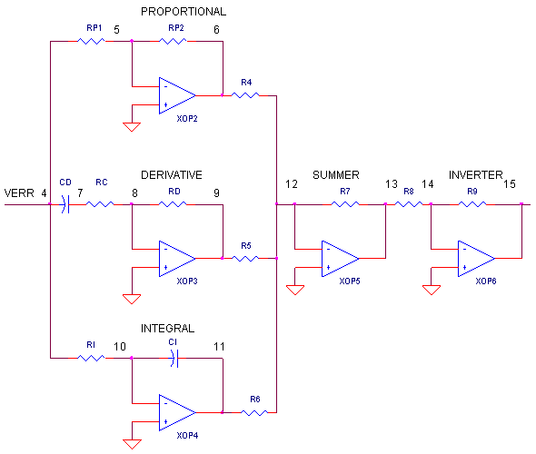
Op Amp PID Controller
CIRCUIT
THE PID CONTROLLER
What basic components are needed for a servo system? Many look similar to the circuit below. The error amp gives you a constant reality check. How? It compares where you want to go, Vset, with where you're at now, Vsensor, by calculating the difference between the two, Verr = Vset - Vsensor. The PID controller takes this error and determines the drive voltage applied to the process in an attempt to bring Vset = Vsensor or Verr = 0.
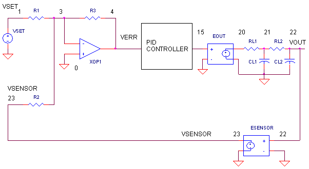
ERROR AMPLIFIER. A classic circuit for calculating the error is a summing op amp. In the controller, XOP1 performs the error calculation. Remembering that the summing amp is an inverting amp, we calculate its output using R1 = R2 = R3 = 10 kΩ.
But how does the summer calculate a difference? Well, it does require that your sensor circuit produce a negative output voltage. Assuming that Vsensor is the negative of the actual sensor voltage Vsensor = - Vsens, you get the difference.Verr = - (Vset / R1 + Vsensor / R2) ∙ R3
= (Vset + Vsensor) ∙ (10 k / 10 k)
= - ( Vset + Vsensor )
You can look at the error amp's function this way. When Vsensor is exactly the negative of Vset, the currents through R1 and R2, equal and opposite, cancel each other as they enter the op amps's summing junction. You end up with zero current through R3 and of course 0V, or zero error, at the output. Any difference between Vset and -Vsensor, results in an error voltage at the output that the PID controller can act upon.Verr = -( Vset - Vsens )
OP AMP PID CONTROLLER. How do we get the PID terms from the error voltage Verr? We enlist three simple op amp circuits. If you need, take a review of the op amp amplifier , integrator and circuit differensiator .
| Term | Op Amp Circuit Function | |
| P | Amplifier: Vo = (RP2 / RP1) ∙ Verr | |
| I | Integrator: Vo = 1/(RI∙CI) ∙ ∫ Verr dt | |
| D | Differentiator: Vo = RD∙CD ∙ dVerr / dt |
Lastly, we need to add the three PID terms together. Again the summing amplifier XOP5 serves us well. Because the error amp, PID and summing circuits are inverting types, we need to add a final op amp inverter XOP6 to make the final output positive, given a positive Vset.
OUTPUT PROCESS. EOUT represents a very simplified model of a process to be controlled, such as motor velocity for example. The gain of 100 could represent an output transfer function of 100 RPM / V. To include the effects of the motor's inertia, we've added some time delay into the output using two cascaded RC filters. Although Vout is simulated in volts, we know it really represents RPM.
SENSOR. The sensor tells you the actual velocity at the motor, 1 V / 100 RPM for this tachometer. ESENSOR models this feedback device. Note, this sensor block actually produces a negative output voltage, the proper input polarity for your error amplifier as mentioned above.
PRE-FLIGHT TEST
Before we close the loop, how do we test our PID terms? Let's apply a signal to the controller and check each term individually. VSET applies a 0.1V step to the error amplifier. Because R2 is initially connected to ground (node 0), the servo loop is essentially opened and the 0.1V step gets applied directly to the PID inputs.
P TEST Run a simulation of the circuit file OP_PID.CIR. Plot the input V(1) and the P Term
at V(6). What voltage should we expect here? With RP2 = 2 kΩ and RP1 = 1 kΩ, you should see a step of
D TEST How much voltage should the derivative term produce? With CD = 0.1 uF, RD = 1 kΩ and a voltage rise of 0.1 V in 0.1 ms, the circuit should reach a peak ofV(6) = V(3) ∙ RP2 / RP1
= 0.1 ∙ 2k / 1 k
= 0.2 V
during the rise time of the step voltage.V(9) = CD ∙ RD ∙ ΔV / Δt
= 0.1 uF ∙ 1 kΩ ∙ 0.1 V / 0.1 ms
= 100 mV
I TEST Finally, let's check the integral term. With RI = 100 MΩ, CI = 1uF, V(3) = 0.1 V and a test time of Δt = 10 ms, the integrator should create a ramp that rises to
at 10 ms. Now that we've developed some confidence in our op amp-based controller, let's take the plunge and close the loop.V(11) = V(3) / (RI ∙ CI) ∙ Δt
= 0.1 V / (100 MΩ ∙ 1 uF) ∙ 10 ms
= 10 μV
TUNING THE PID CONTROLLER
Okay, time to pilot the PID controls. What kind of response are we looking for? Typically, one that's quick and accurate. The initial circuit component values make for a weak P and almost negligible I and D terms. To close the loop, connect R2 to the sensor (node 23) by changing R2 0 3 10k to
R2
23 3 10k
Although there are many PID tuning methods under the sun, here's a
straightforward one to test our controller.1. SET KP. Starting with KP = 5, KI = 0 and KD = 0. Incrementally increase KP to reduce error until the output starts overshooting and ringing significantly.Extend the simulation time to 100 ms in the .TRAN statement and run a new SPICE simulation. Plot the system input V(1) and the sensor output (23). With Vset = 0.1 V, what should we expect at the sensor output? An ideal controller will bring Vsensor = - 0.1V, equal and opposite of Vset, implying 0 error at V(3). If you wish, you can keep an eye on the PID terms by plotting V(6), V(9) and V(11) in another window.
2. SET KD. Increase KD to reduce the overshoot to an acceptable level.
3. SET KI. Increase KI to bring the final error to zero.
SET KP Although the response at V(23) looks smooth, the sensor voltage falls short of -0.1 V. So let's crank up KP. You can do this by either decreasing RP1 or increasing RP2. Let's increase RP2 to 5 kΩ. Hey, things are improving! But instability stirs just beneath the surface in the form of some overshoot and ringing. Push RP2 up to 10 k, 50 k, or more. Yes, you get closer to -0.1 V, but overshoot gets worse. Eventually, your system will become unstable and begin to sing (oscillate). You can back off RP2 to 50 kΩ or so.
SET KD The derivative term counteracts KP to tame the overshoot and ringing. Start increasing RD from 1k to 10 k, 100 k and so on. You should see stability returning in the form of a smoother response at V(23). But too much KD, and you're back to instability.
SET KI With RP2 = 50 kΩ and RD = 100 kΩ, let's kick up the I term to reel in the last bit of error. To do this, you can decrease RI or CI. Start decreasing RI from 100 M, 10 M and so on. At some point you should see the sensor's output start walking closer toward -0.1 V. You might want to put up a cursor to monitor the exact value of V(23). The bigger you make KI, the faster it will move toward -0.1 V. But like the other terms, there's usually a sweet spot that gives you the a reasonable response.
Congratulations, you've earned your junior wings as an op amp PID tuner! Of course, you'll need plenty of hours on a real system before you can say it boldly, but this is a good start.
PID ADJUSTMENTS
In a real circuit, adjusting the PID gains by swapping resistors and capacitors may be cumbersome. Potentiometers make a better choice. But you still may have to swap Rs and Cs to get you in the ballpark. Once there, you have a few options. I've seen one circuit where three pots were hung from node 3 to ground. At the centertaps of each, components RP1, CD and RI were connected. Another incarnation hung three pots, one at the output of each term - nodes 6, 9 and 11 - with their centertaps connected to summer components R4, R5 and R6. Let me know if you come across other useful adjustment methods.
SIMULATION NOTE
To make the PID controller more realistic, a voltage clamp was added to the op amp model. Tacking zener diodes onto the model simulates the output hitting a ±10 V maximum. Why add this feature? Without the clamp, the simulated PID terms may generate hundreds of volts in an attempt to control the output. This may lead to disappointing results when the actual PID outputs get stuck near the supply rails. You can see if any PID terms hit the rail by plotting V(6), V(9) and V(11). What would happen at different clamp levels or without any clamping? You can change the clamp level via the BV parameter in the DZ model or comment out the clamp diodes all together.
THE DERIVATIVE TERM
Of the PID functions, the derivative can be one of the trickier terms. Why? This circuit brings two challenges to the table. 1) Because the circuit is a high-pass filter by nature, it may amplify unwanted noise and disturbances causing an erratic drive signal. To reduce this undesirable effect, resistor RC places a limit on the high frequency gain to Gmax = RD / RC. To further cut the high frequency gain, many circuits include a feedback cap CF across RD. With CF, the circuit begins to look like a low-pass filter at higher frequencies. For a good starting point, pick CF = CD / 10.
2) The second challenge of the derivative circuit is keeping it stable. The classic Op Amp Differentiator may ring or oscillate if not for resistor RC. This resistor reduces the phase-shift caused by RD and CD especially at high frequencies where it can threaten circuit stability. Capacitor CF brings an added bonus of bringing stability to the differentiator. And to boot, CF helps the differentiator recover in case its output is overdriven to the supply rails.
Xsimple with :
SPICE FILE
OP_PID1.CIR - OPAMP PID CONTROLLER
*
* SET POINT
VSET 1 0 PWL(0MS 0MV   0.1MS 0.1V   2000MS 0.1V)
*
* CALCULATE ERROR
R1 1 3 10K
R2 0 3 10K
R3 3 4 10K
XOP1 0 3 4 OPAMP1
*
* P - PROPORTIONAL TERM
RP1 4 5 1K
RP2 5 6 2K
XOP2 0 5 6 OPAMP1
*
* D - DERIVATIVE TERM
CD 4 7 0.1UF
RC 7 8 200
RD 8 9 1K
XOP3 0 8 9 OPAMP1
*
* I - INTEGRAL TERM
RI 4 10 100MEG
CI 10 11 1UF IC=0
XOP4 0 10 11 OPAMP1
*
* SIM PID TERMS
R4 6 12 10K
R5 9 12 10K
R6 11 12 10K
R7 12 13 10K
XOP5 0 12 13 OPAMP1
*
* INVERT SUMMATION
R8 13 14 10K
R9 14 15 10K
XOP6 0 14 15 OPAMP1
*
* PROCESS BLOCK WITH TIME LAG (PHASE SHIFT)
EOUT 20 0 15 0 100
RL1 20 21 10K
CL1 21 0 1UF
RL2 21 22 10K
CL2 22 0 1UF
*
* SENSOR BLOCK (NEG OUT FOR ERROR AMP.)
ESENSOR 23 0 22 0 -0.01
RL3 23 0 10K
*
* OPAMP MACRO MODEL, SINGLE-POLE WITH 10V OUTPUT CLAMP
* connections:      non-inverting input
*                   |   inverting input
*                   |   |   output
*                   |   |   |
.SUBCKT OPAMP1     1   2   6
* INPUT IMPEDANCE
RIN 1 2 10MEG
* DC GAIN=100K AND POLE1=100HZ
* UNITY GAIN = DCGAIN X POLE1 = 10MHZ
EGAIN 3 0 1 2 100K
RP1 3 4 100K
CP1 4 0 0.0159UF
* ZENER LIMITER
D1 4 7 DZ
D2 0 7 DZ
* OUTPUT BUFFER AND RESISTANCE
EBUFFER 5 0 4 0 1
ROUT 5 6 10
*
.model DZ D(Is=0.05u Rs=0.1 Bv=10 Ibv=0.05u)
.ENDS
*
* ANALYSIS
.TRAN  0.1MS 10MS
*
* VIEW RESULTS
.PRINT TRAN V(23)
.PROBE
.END


Plot Y versus time, for three Kp values (Ki and Kd held constant)
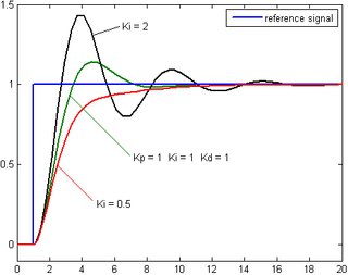
Plot Y versus time, for three Kp values (Ki and Kd held constant)
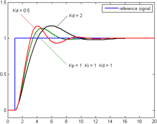
Plot Y vs waktu, untuk 3 nilai Kd (Kp dan Ki dijaga konstan)
X . II PID control
PID controller has been used for more than four centuries in various forms. It has enjoyed popularity as a purely mechanical device, a pneumatic device, and as electronic equipment.
Ments of PID controller raises elements in each sensor electronics also carry out various forms and tasks and have different effects on the functioning of the system work. basically PID or PITa working on an electronic system to minimize errors of ROBO mission performance, especially in a three or four-dimensional space is limited.


tuning PID / PITa
The nice thing about tuning PID controller is that we do not needto have a good understanding of formal control theory to doa pretty good job of it. Approximately 96% of applications closed-loop controllersThe world is currently doing work opportunities PID / PITa was very good indeed with a simple controller that just tuned pretty well. If we can, we are connecting the system to a few test tools, or write in some debugging code to allow us to see three or four variables corresponding finite dimensional variable ROBO mission. If your system enough we could block the slow variables right out on the serial port and graphics desired by using a spreadsheet. if we want to be able to see the drive output devices and output a plant that uses ROBO limited basis. In addition, we want to be able to implement some sort of squarewave, sine wave, longitudinal wave, in which a command signal to the input of our system. It is quite easy to write some test code that will generate the appropriate test command. Once we get the setup ready, set all profits to zero or move dynamically with high efficiency and effectiveness. If we suspect that we will not need differential control (such as Motor and tooth samples or thermal systems) and then jump down to the section that discusses the proportional gain tuning. If we do not start by adjusting the differential reinforcement. The way we coded controller can not use differential control alone. Organize your proportionateget some small value (one or less). Check to see how the system works. If oscillates with a proportional gain then we should be able to heal with differential amplifier to get the right mission. Start with about a hundred times more than the differential gain proportional gain. watch us encouraging signals to become more efficient and effective in ROBO mission. Now start increasing the differential gain until we see the oscillation, excessive noise, or excessive (more than half were destroyed or damaged signal at the output) on a drive or a mission overshoot on the output tool. Note that the oscillation of too much differential gain is much faster than the oscillation of not enough. we want to encourage the gain until the system is on the verge of oscillation then re-gain off by a factor of two or four. Make sure the drive signal still looks good. at this point we will probably system will respond very slowly, so it's time to set the proportional and the advantage inseparable. If it is not set already, set proportional gain initial value between 1 and 100. The system we might be better output performance not to be very slow or will oscillate. If we see the oscillation, drop proportional gain by a factor of eight or ten to oscillation stops. If we do not see oscillation, increase the national propor gain by a factor of eight or 10 until we begin to see the oscillation or excessive overshoot. as with differential controller, we usually aligned to the point too much overshoot then returned to reinforcement by a factor of twoor four. After we close, a good tune with a proportional gain factor of two until we liked what we saw. After that we have a national gain set, began to increase the gain integral. Your initial values may be from 0.0001 to 0.01, respectively. Here again, we want find various advantages inseparable which gives us fast enough performance without too much overshoot and without being too close to the oscillation.Another problem Unless we work on ROBO who worked on the state of the critical situation in two, three or four-dimensional finite, till ROBO work in a stable position and gentle in point right work raised such motion simple plane that is lifted up with smooth and precise both in landing and take off also in flight missions to a stable position.
X . III Climbing with adhesion

examples of applying PID / PITa on a robo fish


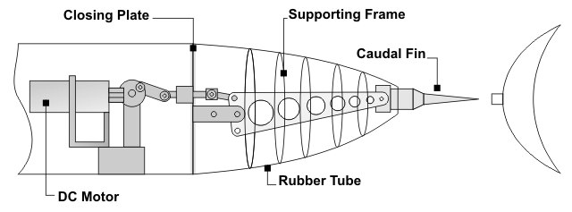

X . IIII PROXIMITY SENSING so PRESSURE SENSING FOR ROBO FISH on ocean wave
Proximity sensing is the ability of a robot to tell when it is near an object, or when something is near it. This sense keeps a robot from running into things. It can also be used to measure the distance from a robot to some object.
The simplest proximity sensors do not measure distance. A bumper can be passive, simply making the robot bounce away from things it hits. More often, a bumper has a switch that closes when it makes contact, sending a signal to the controller causing the robot to back away. When whiskers hit something, they vibrate. This can be detected, and a signal sent to the robot controller.
A photoelectric proximity sensor uses a light-beam generator, a photodetector, a special amplifier, and a microprocessor. The light beam reflects from an object and is picked up by the photodetector. The light beam is modulated at a specific frequency, and the detector has a frequency-sensitive amplifier that responds only to light modulated at that frequency. This prevents false imaging that might otherwise be caused by lamps or sunlight. If the robot is approaching a light-reflecting object, its microprocessor senses that the reflected beam is getting stronger. The robot can then steer clear of the object. This method of proximity sensing won't work for black objects, or for things like windows or mirrors approached at a sharp angle.
An acoustic proximity sensor works on the same principle as sonar. A pulsed signal, having a frequency somewhat above the range of human hearing, is generated by an oscillator . This signal is fed to a transducer that emits ultrasound pulses at various frequencies in a coded sequence. These pulses reflect from nearby objects and are returned to another transducer, which converts the ultrasound back into high-frequency pulses. The return pulses are amplified and sent to the robot controller. The delay between the transmitted and received pulses is timed, and this will give an indication of the distance to the obstruction. The pulse coding prevents errors that might otherwise occur because of confusion between adjacent pulses.
A capacitive proximity sensor uses a radio-frequency ( RF ) oscillator, a frequency detector, and a metal plate connected into the oscillator circuit. The oscillator is designed so that a change in the capacitance of the plate, with respect to the environment, causes the frequency to change. This change is sensed by the frequency detector, which sends a signal to the apparatus that controls the robot. In this way, a robot can avoid bumping into things. Objects that conduct electricity to some extent, such as house wiring, animals, cars, or refrigerators, are sensed more easily by capacitive transducers than are things that do not conduct, like wood-frame beds and dry masonry walls.
Pressure sensing
Pressure sensing allows a robot to tell when it collides with something, or when something pushes against it. Pressure sensors can be used to measure force, and in some cases, to determine the contour of an applied force.
A capacitive pressure sensor employs two metal plates separated by a layer of nonconductive foam. This forms a capacitive transducer . The transducer is connected in series or parallel with an inductor . The resulting inductance-capacitance (LC) combination determines the frequency of an oscillator . If an object strikes or presses against the transducer, the plate spacing decreases, causing the capacitance to increase. This lowers the oscillator frequency. When the pressure is removed, the foam springs back, the plates return to their original spacing, and the oscillator returns to its original frequency. A capacitive pressure sensor can be fooled by metallic objects. If a good electrical conductor comes very close to the plates, the capacitance might change even if physical contact is not made. If this occurs, the sensor will interpret this proximity as pressure.
An elastomer pressure sensor solves the proximity problem inherent in the capacitive device. The elastomer is a foam pad with resistance that varies depending on how much it is compressed. An array of electrodes is connected to the top of the pad; an identical array is connected to the bottom. Each electrode in the top matrix receives a negative voltage, and its mate in the bottom matrix receives a positive voltage. When pressure appears at some point on the pad, the material compresses at and near that point, reducing the resistance between certain electrode pairs. This causes a current increase in a particular region in the pad. The location of the pressure can be determined according to which electrode pairs experience the increase in current. The extent of the pressure can be determined by how much the current increases. If the electrode matrix is fine enough, the contour of the pressure-producing object can be determined by a microprocessor that evaluates the electrode current profile.
The output of a pressure sensor is analog , but it can be converted to digital data using an analog-to-digital converter ( ADC ). This signal can be used by a robot controller. Pressure on a transducer in the front of a robot might cause the machine to back up; pressure on the right side might make the machine turn left. The presence of pressure might be used to actuate an alarm, or to switch a device on or off. Calibrated pressure sensors can be used to measure applied force, mass, weight, or acceleration.
A back-pressure sensor is a transducer that detects and measures the instantaneous torque that a robot motor applies. The sensor produces a variable signal, usually a voltage , that changes in a linear manner as the torque varies.
When a robot motor operates, it encounters mechanical resistance. This resistance might depend on lifted mass, mechanical friction against a surface or within a system, or the opposition to applied force caused by electromagnetic interaction (as in an electric generator). Torque is the turning force that a robot motor delivers. It is important that a robot motor provide enough torque to overcome the resistance in external systems, but excessive torque can be destructive.
A robot motor produces a measurable back pressure that depends on the applied torque. The greater the torque, the greater the back pressure, and the greater the output of the back-pressure sensor. This output, called the back signal or back voltage, can be used in a feedback loop to reduce the torque applied by the motor. The loop configuration acts as a force limiter that minimizes the possibility of damage to objects handled by a robotic end effector. The force limiter can also reduce the chance of injury to personnel working around the robot.
In robotics, an end effector is a device or tool that's connected to the end of a robot arm where the hand would be. The end effector is the part of the robot that interacts with the environment. The structure of an end effector and the nature of the programming and hardware that drives it depend on the task the robot will be performing.
In manufacturing, a robot arm can accommodate only certain tasks without changes to its end effector's ancillary hardware and/or programming. If a robot needs to pick something up, a type of robot hand called a gripper is the most functional end effector. If a robot needs to be able to tighten screws, however, then the robot must be fitted with an end effector that can spin.
End effectors used in manufacturing include:
- anti-collision sensors
- brushes
- cameras
- cutting tools
- drills
- grippers
- magnets
- sanders
- screw drivers
- spray guns
- vacuum cups
- welding guns
Eye in hand system
An eye-in-hand system is a robot end effector equipped with a close-range camera. The camera is designed for work at distances from a fraction of a millimeter to approximately one meter. A lamp is included in the gripper (robot hand) along with the camera to ensure that a good image is obtained in dim light. The camera has a lens that can be adjusted for proper focus, so the positioning error is minimized.
Eye-in-hand systems are used primarily to guide robot end effectors and grippers, and to ensure that grippers properly engage the intended targets. The system can also precisely measure the distance from the end effector or gripper to a target. In a robot equipped with a smart controller, the eye-in-hand system allows positive identification of a target. The controller compares the image from the camera with a set of images stored in memory.
motion plan
A motion plan is a multi-step process that can be used by a robot to precisely position itself to perform a specified task. Suppose you own an autonomous mobile personal robot. You tell it to switch on the light in a bedroom. The light switch is on the wall. The robot has a computer map of the house stored in its controller memory. This three-dimensional map includes the exact coordinates of the bedroom light switch, and/or its position relative to other objects. The robot first proceeds to the general location of the switch. The program that facilitates this is known as a gross-motion plan.
In order to find the switch, and to position its end-effector (robot hand) in the right place to toggle it, a fine-motion plan is required. Machine vision can facilitate this. An example is the so-called eye-in-hand system, which allows the robot to recognize the shape of the switch and guide the end effector into place, down to millimeter displacements or smaller. Another method of executing the fine-motion plan involves tactile sensing, in which the robot's end effector gropes along the wall until it finds and throws the switch, just as you could find and throw it with your eyes closed once you were in its general vicinity.
grasping plan
A grasping plan is an algorithm used by a robot arm and gripper to get hold of a specific object. The details of such a program depend on the type of robot arm and gripper, on the size of the robot's work area, and on the type of object(s) to be grasped.
As an example, imagine you own a mobile, autonomous personal robot. You are having spaghetti with lots of sauce for supper, so you feel compelled to instruct the machine to get you six paper napkins. The robot must use a certain program to find the kitchen, another program to locate the cabinet or drawer in which the napkins are stored, and another program to determine which objects in the drawer are the paper napkins. Then the gripper must pick up exactly six napkins without upsetting the other contents of the drawer or cabinet. This is a simple process for a human being, even a child, to carry out, but it is complex when reduced to digital components. There are myriad ways in which the robot might execute this assignment wrong, but only one way to do it right.
A grasping plan can be enhanced by machine vision . Tactile sensors, pressure sensors, and texture sensors can also help ensure that the gripper picks up the correct object in the right way. An efficient and reliable grasping plan involves the use of a detailed, three-dimensional map of the robot's entire work environment, stored in the robot controller's memory. The grasping plan can then assign every object or set of objects a range of coordinate values.
theory and design of robots in various shapes pointing and refer to:
1. Robots should not be harmful to humans.
2. A robot must follow the instructions of human being without breaking the rules first.
3. A robot must protect themselves without violating other rules.
4. The robot can carry out the instructions in a timely and continued instruction
the next logical understanding of mission work.
X . IIIII Proportional amplifier on wish output good performance

It's no secret that it takes a lot of knowledge to really understand the world of audio and video in the strengthening of proportional or commonly referred to as amplifier alone, filled with confusing numbers and terms. example: Watt, the current time, distortion, frequency and impedance are just a few of the specs are looking for a home theater receiver amplifier will come and use dynamic motion robot. With thousands of choices in each category, it takes a little background to use this specification to make a choice.
In steps the watt...
Evaluating and stating the wattage of an amplifier has become the single most important number to the amplifier shopper. Unfortunately, wattage is a highly misunderstood specification, which dupes people into buying products with a level of performance much lower than what is anticipated. 100 watts seems to be the magic number for most, thinking that as long as you have 100 of them, and no less, they'll be fine. However, even passenger side mirror on your car states that things aren't always as they appear.To be fair, wattage is an important number that can give a clear understanding of an amplifiers performance. A Watt, named after the British scientist James Watt, is a unit of power. And since power is expressed as a unit of energy divided by a unit of time, a watt is commonly defined as a unit of power equal to one joule per second. Simply stated, a watt is the amplifiers ability to do work, like make the drivers in a loudspeaker move.
Wattage in an amplifier is like horsepower in a car. The more horsepower a car has, the faster the car goes. But unfortunately, this isn't always true. Take into consideration that a 150 horsepower engine might be able to rocket a 1200-pound car, but it's not going to budge a 5-ton semi-truck. The weight of the car is similar to the weight (efficiency) of the speaker connected to an amplifier.
Standardizing the Specs (sort of...)
In the competitive atmosphere that has taken over the entire electronics industry, manufacturers and marketers struggle to make their products appeal to the masses. Of which, massaging the specifications of their products is a sure fire way to attract buyers in a sea filled with similar products.There is, to this day, no truly defined way to measure the power output of an amplifier. As you will learn below, the numbers do not mean much until they can be understood in context, and broken down in a manner that allows fair comparisons between products.
When amplifiers went from tube amplifiers (that use vacuum tubes) to solid-state amplifiers, power ratings for amplifiers got extremely confusing. Finally, the FTC stepped in ruled that all power claims had to include the conditions in which they were measured. Unfortunately, the FTC did not rule that amplifiers had to be tested on the same playing field. This means that in order to make fair comparisons, one would need to know how to interpret what the conditions of the measurement means. Specifically, the FTC ruled that:
- Power measurements must be stated in RMS (sustained) watts.
- The bandwidth (band of frequencies) used in the measurement must be stated.
- The impedance (load) had to be stated.
- The number of amplifier channels played into that load had to be stated.
- Total harmonic distortion figures had to be stated.
Specifications Explained
More often than not, looking at amplifier specifications can reveal a great deal about the amplifiers real world performance. Below is an explanation of each specification, and how to interpret them.-
RMS Power
There are two ways of expressing power, peak and RMS. Peak power is
the amplifier's ability to provide an instantaneous burst of power.
However, peak power measurements are somewhat fictitious since they
cannot be sustained for long. RMS (Root Mean Square)
power ratings are a mathematically correct way to express an
amplifier's usable average power, which is a representation of
real-world performance. -
Bandwidth
Bandwidth refers to the frequency range used to produce the claimed
power specification. Most amplifiers have a harder time producing the
frequency extremes, such as low bass frequencies or high treble, than it
does with midrange frequencies. Humans with perfect hearing can discern
a frequency range from 20Hz to 20kHz (20,000Hz). Since music and movie
soundtracks involve a very wide range of frequencies, it is good to know
what range the amplifier was tested under. This ensures that the
amplifier can hold its own producing the dynamic effects of music and movies. -
Impedance
Solid-state amplifiers usually produce lower wattage into higher
impedances (electrical resistance) than lower impedances. This, however,
is not always true for tube amplifiers. -
Number of Channels Driven
Long ago, when amplifiers had only two channels, the term "all
channels driven" meant that the test included both amplifiers being
tested simultaneously. Today, products contain 5, 7, or even 10
amplifiers in one chassis, and this term can be a bit deceiving. It
would make sense that "all channels driven" would mean that every
channel in the product were all tested simultaneously, but
unfortunately, this is not always true. -
Total Harmonic Distortion (THD)
Distortion measurements do not necessarily speak volumes. At some
degree or another, all amplifiers introduce distortion, which is when an
amplifier changes the input signal.
In most cases, the distortion increases as the power demanded grows.
Distortion measurements can give an indication of when an amplifier is
operating in a non-linear fashion.
Many manufacturers often try to massage the specifications of amplifiers to give them a higher claimed wattage. When you see a power rating that says "x watts @ 1 kHz", it means that they only tested one specific frequency to get its power rating. Not only does this not give you any indication of whether or not the amplifier can hold its own during frequency extremes, but it is unfair to buyers since the measured wattage would be considerably less if all frequencies had been used.
According to Ohm's Law, a perfect amplifier would produce twice the wattage into a 4-ohm load than it does into an 8-ohm load. But since lower loads can drain amplifiers quickly, the power supplies tend to produce less operating voltage. So in the real world, lowering the impedance of the speaker will not necessarily yield twice the wattage from the receiver.
This is another way that manufacturers can fool consumers. When evaluating power specifications, the output wattage will typically be larger when a lower impedance is used for testing.
Manufacturers can cheat a little bit when testing the wattage of a receiver. If, for example, a product contains 7 amplifiers, yet they only used two of them at the same time while testing, the claimed wattage on the receiver would be significantly higher than if all 7 amplifiers had been used. It is important to read the fine print to find out exactly how many amplifiers had been used for the test.
Manufacturers can also use this specification to their advantage. As stated above, claimed wattage is the effect of the test variables. So, if the manufacturer chooses to turn up an amplifier until it reaches 10% THD, they could report a higher wattage (even though it would probably sound terrible). High wattage at very low distortion is desirable.
how to sort and classify proportional amplifiers or amplifier alone
Manufacturers can be somewhat deceptive about amplifiers, especially the ones in the bargain section of your local electronics store. Below are some general things to look out for when shopping for an amplifier.
When comparing specifications, try as hard as possible to bring them to the same playing field. So, if one amp has a 6-ohm rating and the other an 8-ohm rating, tell yourself that the 6-ohm rating was used for a reason, and that the wattage would be lower if an 8-ohm load had been used.
As we learned above, a perfect amp would produce twice the power into a 4-ohm load as it would into an 8-ohm load. That being said, a perfect amp would produce 1.5 times the power into a 6-ohm load as it would into an 8-ohm load. However, we all know that power supply limitations make this untrue. Be conservative in your estimates. In the examples above, if you decide to state amp #2 as 8-ohms you could divide 100 watts by 1.5 to get an answer of 66 watts. However, remember that the manufacturer avoided the low bass frequencies, so the true power output may only be around 55 watts (depending on the power supply) if full range speakers are used.
Amplifiers that claim "x watts @ 1 kHz" should not be trusted. Their real world performance could be less than half of what the claimed power specifications say. The test bandwidth for any power claim should be at least "x-watts @ 20Hz-20kHz).
Amplifiers with "one channel driven" should not be trusted. It indicates a serious problem with the amplifier's ability to produce high wattage under real conditions.
Be cautious if someone tries to sell you on fictitious "peak" power ratings. While they might seem impressive, they say nothing about how the amplifier actually performs.
Watch out for distortion ratings. Within limits, lower numbers are more desirable, but usually anything under 1% is inaudible.
Keep in mind the speakers that will be connected to the amplifier. If you have big, high quality speakers, an inexpensive amplifier probably is not going to help you get the most out of them. Likewise, there is no reason to go overboard on an amplifier for inexpensive speakers.
When shopping for an integrated receiver (where there is processing and amplification in one box), keep in mind that there are other features that may be just as important as the watts as mentioned above.
Price is not always a clear indication of amplifier quality. However, in many cases, there are reasons why great performing amplifiers come with a higher than expected price tag.


Tidak ada komentar:
Posting Komentar