All life processes always begin and are initiated by the concept of attraction (Push and Pull), some of which are:
1. Love which is the attraction between men and women
towards the stability of body and soul.
2. energy conservation where the numerical value of energy moves in a manner
push - pull goes to neutral ie 0 (null or void) or
the harmonization process also leads to core stability although it can
into a different form but the taste is the same.
3. read and write memory and copy paste which is
Data collection (Push) also processes data into results
Legitimate information is a mechanism (Pull).
4. Push (collect) and delete (Pull).
5. electronic circuits which are also systems of attraction
where energy will turn into motion, light, indicators
and heat is also a magnet until such a function is stable
Batteries, batteries, adapters (there are harmonizations 1, 2, 3, 4 are called
ripple), electronic components and their circuit pathways.
6. Space is also a process of attraction of various kinds
kinds of harmonizing forces and energies that move in space
and time so that they experience emptiness or vacuum,
or we can call space is a neutral zone (0)
Gen. Mac Tech to operation and change operation
1

( AMNIMARJESLO SAN )
2
⇉ Push–pull Input / Output ⇇

A push–pull in electronic is a concept of attraction in electronics is a special concept because all electronic components function due to the attractive relationship between positive and negative electrons, as well as the attraction of photons in the electronic components of light. Thus humans in life there is also the process of attraction that is love.
electronic circuit
that uses a pair of active devices that alternately supply current to,
or absorb current from, a connected load. Push–pull outputs are present
in TTL and CMOS digital logic circuits and in some types of amplifiers, and are usually realized as a complementary pair of transistors, one dissipating or sinking current from the load to ground or a negative power supply, and the other supplying or sourcing current to the load from a positive power supply ,
Push–pull circuits are widely used in many amplifier output stages .
Push–pull transistor output stages :
Categories include:
Transformer-output transistor power amplifiers
It
is now very rare to use output transformers with transistor amplifiers,
although such amplifiers offer the best opportunity for matching the
output devices (with only PNP or only NPN devices required).
Totem pole push–pull output stages
Two
matched transistors of the same polarity can be arranged to supply
opposite halves of each cycle without the need for an output
transformer, although in doing so the driver circuit often is asymmetric
and one transistor will be used in a
common-emitter configuration while the other is used as an
emitter follower.
This arrangement is less used today than during the 1970's; it can be
implemented with few transistors (not so important today) but is
relatively difficult to balance and to keep a low distortion.
Symmetrical push–pull
Each half of the output pair "mirror" the other, in that an NPN (or N-Channel
FET) device in one half will be matched by a PNP (or P-Channel
FET)
in the other. This type of arrangement tends to give lower distortion
than quasi-symmetric stages because even harmonics are cancelled more
effectively with greater symmetry.
Quasi-symmetrical push–pull
In
the past when good quality PNP complements for high power NPN silicon
transistors were limited, a workaround was to use identical NPN output
devices, but fed from complementary PNP and NPN driver circuits in such a
way that the combination was close to being symmetrical (but never as
good as having symmetry throughout). Distortion due to mismatched gain
on each half of the cycle could be a significant problem.
Super-symmetric output stages
Employing
some duplication in the whole driver circuit, to allow symmetrical
drive circuits can improve matching further, although driver asymmetry
is a small fraction of the distortion generating process. Using a
bridge-tied load
arrangement allows a much greater degree of matching between positive
and negative halves, compensating for the inevitable small differences
between NPN and PNP devices.
Square-law push–pull
The output devices, usually
MOSFETs or
vacuum tubes, are configured so that their
square-law transfer characteristics (that generate second-harmonic
distortion
if used in a single-ended circuit) cancel distortion to a large extent.
That is, as one transistor's gate-source voltage increases, the drive
to the other device is reduced by the same amount and the drain (or
plate) current change in the second device approximately corrects for
the non-linearity in the increase of the first.
Push–pull tube (valve) output stages
Vacuum tubes
(valves) are not available in complementary types (as are pnp/npn
transistors), so the tube push–pull amplifier has a pair of identical
output tubes or groups of tubes with the
control grids
driven in antiphase. These tubes drive current through the two halves
of the primary winding of a center-tapped output transformer. Signal
currents add, while the distortion signals due to the non-linear
characteristic curves
of the tubes subtract. These amplifiers were first designed long before
the development of solid-state electronic devices; they are still in
use by both
audiophiles and musicians who consider them to sound better.
Vacuum tube push–pull amplifiers usually use an output transformer, although
Output-transformerless (OTL) tube stages exist (such as the SEPP/SRPP and the White Cathode Follower below).
The phase-splitter stage is usually another vacuum tube but a
transformer with a center-tapped secondary winding was occasionally used
in some designs. Because these are essentially square-law devices, the
comments regarding
distortion cancellation mentioned
above apply to most push–pull tube designs when operated in
class A (i.e. neither device is driven to its non-conducting state).
A
Single Ended Push–Pull (
SEPP,
SRPP or
mu-follower) output stage, originally called the
Series-Balanced amplifier
(US patent 2,310,342, Feb 1943). is similar to a totem-pole arrangement
for transistors in that two devices are in series between the power
supply rails, but the input drive goes
only to one of the devices,
the bottom one of the pair; hence the (seemingly contradictory)
Single-Ended description. The output is taken from the cathode of the
top (not directly driven) device, which acts part way between a constant
current source and a cathode follower but receiving some drive from the
plate (anode) circuit of the bottom device. The drive to each tube
therefore might not be equal, but the circuit tends to keep the current
through the bottom device somewhat constant throughout the signal,
increasing the power gain and reducing distortion compared with a true
single-tube single-ended output stage.
The
White Cathode Follower (Patent 2,358,428, Sep 1944 by E. L. C. White) is similar to the SEPP design above, but the signal input is to the
top
tube, acting as a cathode follower, but one where the bottom tube (in
common cathode configuration) if fed (usually via a step-up transformer)
from the current in the plate (anode) of the top device. It essentially
reverses the roles of the two devices in SEPP. The bottom tube acts
part way between a constant current sink and an equal partner in the
push–pull workload. Again, the drive to each tube therefore might not be
equal.
Transistor versions of the SEPP and White follower do exist, but are rare.
Ultra-linear push–pull
A so-called
ultra-linear push–pull amplifier uses either
pentodes or
tetrodes with their
screen grid
fed from a percentage of the primary voltage on the output transformer.
This gives efficiency and distortion that is a good compromise between
triode (or
triode-strapped)
power amplifier circuits and conventional pentode or tetrode output
circuits where the screen is fed from a relatively constant voltage
source.
Push–pull converter
A push–pull converter is a type of DC-to-DC converter, a switching converter that uses a transformer to change the voltage
of a DC power supply. The distinguishing feature of a push-pull
converter is that the transformer primary is supplied with current from
the input line by pairs of transistors in a symmetrical push-pull circuit.
The transistors are alternately switched on and off, periodically
reversing the current in the transformer. Therefore, current is drawn
from the line during both halves of the switching cycle. This
contrasts with buck-boost converters,
in which the input current is supplied by a single transistor which is
switched on and off, so current is only drawn from the line during half
the switching cycle. During the other half the output power is supplied
by energy stored in inductors or capacitors in the power supply.
Push–pull converters have steadier input current, create less noise on
the input line, and are more efficient in higher power applications.

Push-pull converter (+12V → ±18V; 50W) as potted module. ① transformer; ② and ③ electrolytic capacitors vertical and horizontal mounted; ④ discrete circuit board in through-hole technology .
Circuit operation

Conceptual schematic of a full-bridge converter. This is not a center tapped or split primary push-pull converter.
Top: Simple inverter circuit shown with an
electromechanical switch
and automatic equivalent
auto-switching device implemented with two transistors and split winding auto-transformer in place of the mechanical switch.
The term
push–pull is sometimes used to generally refer to any
converter with bidirectional excitation of the transformer. For
example, in a full-bridge converter, the switches (connected as an
H-bridge)
alternate the voltage across the supply side of the transformer,
causing the transformer to function as it would for AC power and produce
a voltage on its output side. However,
push–pull more commonly refers to a two-switch topology with a split primary winding.
In any case, the output is then rectified and sent to the load.
Capacitors are often included at the output to filter the switching noise.
In practice, it is necessary to allow a small interval between
powering the transformer one way and powering it the other: the
“switches” are usually pairs of transistors (or similar devices), and
were the two transistors in the pair to switch simultaneously there
would be a risk of shorting out the power supply. Hence, a small wait is
needed to avoid this problem. This wait time is called "Dead Time" and
is necessary to avoid transistor shoot-through.
Transistors
N-type
and P-type power transistors can be used. Power MOSFETs are often
chosen for this role due to their high current switching capability and
their inherently low ON resistance. The gates or bases of the power
transistors are tied via a resistor to one of the supply voltages.
A P-type transistor is used to pull up the N-type power transistor gate (
common source) and an N-type transistor is used to pull down the P-type power transistor gate.
Alternatively, all power transistors can be N-type, which offer
around three times the gain of their P-type equivalents. In this
alternative the N-type transistor used in place of the P-type has to be
driven in this way:
The voltage is amplified by one P-type transistor and one N-type
transistor in
common base configuration to rail-to-rail amplitude.
Then the power transistor is driven in
common drain configuration to amplify the current.
In high frequency applications both transistors are driven with
common source.
The operation of the circuit means that both transistors are
actually pushing, and the pulling is done by a low pass filter in
general, and by a center tap of the transformer in the converter
application. But because the transistors push in an alternating fashion,
the device is called a push-pull converter.
Timing
If both
transistors are in their on state, a short circuit results. On the other
hand, if both transistors are in their off state, high voltage peaks
appear due to back EMF.
If the driver for the transistors is powerful and fast enough,
the back EMF has no time to charge the capacity of the windings and of
the body-diode of the
MOSFETs to high voltages.
If a microcontroller is used, it can be used to measure the peak
voltage and digitally adjust the timing for the transistors, so that the
peak only just appears. This is especially useful when the transistors
are starting from cold with no peaks, and are in their boot phase.
The cycle starts with no voltage and no current. Then one
transistor turns on, a constant voltage is applied to the primary,
current increases linearly, and a constant voltage is induced in the
secondary. After some time T the transistor is turned off, the parasitic
capacities of the transistors and the transformer and the
inductance of the transformer form an
LC circuit
which swings to the opposite polarity. Then the other transistor turns
on. For the same time T charge flows back into the storage capacitor,
then changes the direction automatically, and for another time T the
charge flows in the transformer. Then again the first transistor turns
on until the current is stopped. Then the cycle is finished, another
cycle can start anytime later. The S-shaped current is needed to improve
over the simpler converters and deal efficiently with
remanence.
3
⇉The conservation of energy on push - pull⇇
When you do a useful job with a force (a push or a pull), such as moving a car uphill, we say you're doing work, and that takes energy. ... So no energy is created or destroyed here: you're simply converting energy stored as fuel inside your body into potential energy stored by the car (because of its height).
Cars can pull off the same trick.
Depending on which make and model you own, you probably know that it
does so many kilometers or miles to the gallon; in other words, using
a certain amount of energy-rich gasoline, it can transport you (and a
moderate load) a certain distance down the road. What we have here
are two examples of machines—the human body and the automobile—that
obey one of the most important laws of physics: the conservation of
energy. Written in its simplest form, it says that you can't create
or destroy energy, but you can convert it from one form into another.
Pretty much everything that happens in the universe obeys.
What is the conservation of energy?
The first thing we need to note is that the law of conservation of
energy is completely different from
energy conservation.
Energy conservation means saving energy through such things as
insulating your home or using public transportation; generally it
saves you money and helps the planet. The conservation of energy has
nothing to do with saving energy: it's all about where energy comes
from and where it goes.
Write the law formally and it sounds like this:
In a closed system, the amount of energy is fixed. You can't create any more energy
inside the system or destroy any of the energy that's already in there. But you
can convert the energy you have from one form to another (and
sometimes back again).
A "closed system" is a bit like a sealed box
around whatever we're studying: no energy can leak into the box from the inside (or be introduced to the box from outside).
There are some even simpler, more familiar ways of stating the conservation
of energy. "No pain, no gain" is a rough everyday equivalent: if
you want something, you have to work for it. "There's no such thing
as a free lunch" and "You don't get anything for free" are
other examples.
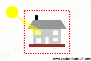 Artwork: This house is an example of a closed
system: the energy that's inside the red dotted line stays as it is or
gets converted into other forms. We can't create any new energy inside
the house out of nothing at all, and we can't make energy inside the
house vanish without trace, though we can turn it into other forms. So
what if one room of the house suddenly starts getting hotter? The heat
energy making that happen must be coming from energy that's already
inside the house in a different form (maybe it's wood in a fire that's
being burned to release the chemical energy locked inside it). If that's
not the case, we don't have a closed system: the "extra" heat must be
coming into the house from outside (maybe strong sunlight streaming in
through the window).
Artwork: This house is an example of a closed
system: the energy that's inside the red dotted line stays as it is or
gets converted into other forms. We can't create any new energy inside
the house out of nothing at all, and we can't make energy inside the
house vanish without trace, though we can turn it into other forms. So
what if one room of the house suddenly starts getting hotter? The heat
energy making that happen must be coming from energy that's already
inside the house in a different form (maybe it's wood in a fire that's
being burned to release the chemical energy locked inside it). If that's
not the case, we don't have a closed system: the "extra" heat must be
coming into the house from outside (maybe strong sunlight streaming in
through the window).
Examples of the conservation of energy
The conservation of energy (and the idea of a "closed system") sounds
a bit abstract, but it becomes an awful lot clearer when we consider
some real-life examples.
Driving a car
Fill a car up with gasoline and you have a closed system. All the energy you
have at your disposal is locked inside the gas in your tank in
chemical form. When the gas flows into your
engine, it burns with
oxygen in the air. The chemical energy in the gas is converted first
into
heat energy: the burning fuel makes hot expanding gas, which
pushes the pistons in the engine cylinders. In this way, the heat is
converted into mechanical energy. The pistons turn the crankshaft,
gears, and driveshaft and—eventually—the car's
wheels. As the wheels turn, they speed the vehicle along the road, giving it kinetic energy (energy of movement).
If a car were 100 percent efficient, all the chemical energy originally locked
inside the gasoline would be converted into kinetic energy.
Unfortunately, energy is wasted at each stage of this process.
Some is lost to friction when metal parts rub and wear against one
another and heat up; some energy is lost as
sound
(cars can be quite noisy—and sound is energy that has to come from somewhere)
Not all the energy the car produces moves you down the road: quite a lot has to
push against the air (so it's lost to air resistance or drag), while
some will be used to power things like the headlights,
air
conditioning, and so on. Nevertheless, if you measure the energy you
start with (in the gasoline) and calculate how much energy you finish
with and lose on the way (everything from useful kinetic energy and
useless energy lost to friction, sound, air resistance, and so on),
you'll find the energy account always balances: the energy you start
with is the energy you finish with.
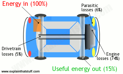 Artwork: Like everything else, cars must obey
the law of conservation of energy. They convert the energy in fuel into
mechanical energy that moves you down the road, but waste quite a lot of
energy in the process. If you put 100 units of energy into a car (in
the form of fuel), only 15 units or so move you down the road. The rest
is wasted as heat losses in the engine (74 percent); parasitic losses
(6%, making electricity, for example, to light the headlamps); and
drivetrain losses (5%, sending power to the wheels). The 15 useful units
of energy are used to overcome drag (air resistance), friction (in the
brakes), and rolling resistance (in the tires). Every bit of energy we
put into a car has to go somewhere, so the energy outputs (74% + 6% + 5%
+ 15%) must always exactly add up to the original energy input (100%).
Figures for city driving from Where the energy goes, fueleconomy.gov.
Artwork: Like everything else, cars must obey
the law of conservation of energy. They convert the energy in fuel into
mechanical energy that moves you down the road, but waste quite a lot of
energy in the process. If you put 100 units of energy into a car (in
the form of fuel), only 15 units or so move you down the road. The rest
is wasted as heat losses in the engine (74 percent); parasitic losses
(6%, making electricity, for example, to light the headlamps); and
drivetrain losses (5%, sending power to the wheels). The 15 useful units
of energy are used to overcome drag (air resistance), friction (in the
brakes), and rolling resistance (in the tires). Every bit of energy we
put into a car has to go somewhere, so the energy outputs (74% + 6% + 5%
+ 15%) must always exactly add up to the original energy input (100%).
Figures for city driving from Where the energy goes, fueleconomy.gov.
Now this only applies if your car is a "closed system." If you're driving
along the straight and the road suddenly starts going downhill, you're
going to be able to go much further than you'd be able to go
otherwise. Does this violate the conservation of energy? No, because
we're no longer dealing with a closed system. Your car is gaining
kinetic energy from the gasoline in its tank, but it's also gaining
kinetic energy because it's going downhill. This isn't a closed
system so the conservation of energy doesn't apply anymore.
Boiling a kettle
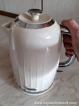 Photo: An electric kettle like this converts
electrical energy into heat energy.
That's the reverse of the process
that happens in the power plant that supplies your home, where electricity is produced using heat energy released by burning a fuel such as coal, oil, or gas.
Photo: An electric kettle like this converts
electrical energy into heat energy.
That's the reverse of the process
that happens in the power plant that supplies your home, where electricity is produced using heat energy released by burning a fuel such as coal, oil, or gas.
Boil
water with an
electric kettle and you're seeing the conservation of
energy at work again. Electrical energy drawn from the power outlet
on your wall flows into the
heating element in the base of your
kettle. As the current flows through the element, the element rapidly
heats up, so the electrical energy is converted into heat energy that
gets passed to the cold water surrounding it. After a couple of
minutes, the water boils and (if the power stays on) starts to turn
to steam. How does the conservation of energy apply here? Most of the
electrical energy that enters the kettle is converted into heat
energy in the water, though some is used to provide
latent heat of
evaporation (the heat we need to give to liquids to turn them into
gases such as steam). If you add up the total electrical energy
"lost" by the electricity supply and the total energy gained by
the water, you should find they're almost exactly the same. Why
aren't they
exactly equal? Simply because we don't have a
closed system here. Some of the original energy is converted to sound
and wasted (kettles can be quite noisy). Kettles also give off some
heat to their surroundings—so that's also wasted energy.
Pushing a car uphill
In the everyday world, "work" is something you do to earn money; in physics,
work has a different meaning. When you do a useful job with a force (a push or a pull),
such as moving a car uphill, we say you're
doing work,
and that takes energy. If you push a car uphill, it has more potential energy
at the top of the hill than it had at the bottom. Have you violated the
conservation of energy by creating potential energy out of thin air?
No! To push the car, you have to do work against the force of gravity.
Your body has to
use energy to do work.
Most of the energy your body uses is gained by the car as you push it uphill.
The energy your body loses is pretty much equal to the work it does against gravity.
And the energy the car gains is the same as the work done. So no energy is created or destroyed here:
you're simply converting energy stored as fuel inside your body into potential
energy stored by the car (because of its height).
Who discovered the conservation of energy?
How do we know the conservation of energy is true? First, it sounds
sensible. If you put a heavy log on a fire it might burn for an hour.
If you put a second log, roughly the same size, on the fire, it's
reasonable to suppose you'll get twice as much heat or the fire will
burn twice as long. By the same token, if five bananas can supply
your body with an hour's energy, ten bananas should keep you running
for two hours—although you might not enjoy guzzling them all at
once! In other words, the energy in (the logs you add to the fire or the
bananas you eat) is equal to the energy out (the heat you get by
burning logs or the energy you make by eating bananas).
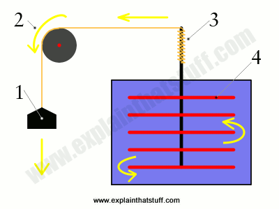 Photo: The Mechanical Equivalent of Heat: In
James Prescott Joule's famous experiment, a falling weight (1) pulls on a
rope that passes over a pulley (2). The rope spins an axle
(3) that turns
a paddle inside a sealed container of water (4). As the paddle spins,
the water heats up. Joule proved that the heat energy gained by the
water was exactly the same as the potential energy lost by the weight.
Photo: The Mechanical Equivalent of Heat: In
James Prescott Joule's famous experiment, a falling weight (1) pulls on a
rope that passes over a pulley (2). The rope spins an axle
(3) that turns
a paddle inside a sealed container of water (4). As the paddle spins,
the water heats up. Joule proved that the heat energy gained by the
water was exactly the same as the potential energy lost by the weight.
“... the quantity of heat produced by the friction of bodies, whether solid or liquid,
is always proportional to the quantity of force expended.”
James Prescott Joule, The Mechanical Equivalent of Heat, 1845.
Reasonable guesswork doesn't quite cut the mustard in science. Really, we need
to be sure that the energy we start with in a closed system is the
same as the energy we end up with. So how do we know this? One of the
first people to confirm the law of conservation of energy
experimentally was English physicist
James Prescott Joule
(1818–1889), who used an ingenious bit of apparatus to find what he
called "the mechanical equivalent of heat." He used a falling
weight to drive a large paddle wheel sealed inside a container of
water. He calculated the potential energy of the weight (the energy
it had because of its height above Earth) and reasoned that, as the
weight fell, it transferred pretty much all its energy to kinetic
energy in the paddle wheel. As the paddle wheel turned, it stirred
the water in the container and warmed it up by a small but
significant amount. Now we know how much energy it takes to warm a
certain mass of water by a certain number of degrees, so Joule was
able to figure out how much energy the water had gained. To his
delight, he found out that this figure exactly matched the energy
lost by the falling weight. Joule's brilliant work on energy was
recognized when the international scientific unit of energy (the
joule) was named for him.
Joule built on earlier work by Anglo-American physicist
Benjamin Thompson (1753–1814),
also known as Count Rumford. While working in a Germany artillery factory, Rumford noted that cannon barrels got hot when they
were being drilled out. He swiftly realized that the heat was not a magic property of the metal (as many people supposed)
but came from the mechanical, frictional process of drilling: the more you drilled, the hotter the metal got.
Rumford's simple calculations produced results that, according to Joule, were "not very widely different
from that which I have deduced from my own experiments." That was a sign both men were on
the right track.
Why perpetual motion machines never work
Back in the 19th century, charlatan inventors would pop up from time to time
showing off miracle machines that seemed to be able to drive
themselves forever. Inventions like this are called
perpetual
motion machines: they seem to be able to move forever without
anyone adding any more energy. Often, machines like this were
blatant tricks: the mechanisms were powered by a concealed assistant
who sat in the shadows turning a hidden handle! Some of the
machines sound plausible, but all of them unfortunately fall foul
of the conservation of energy.
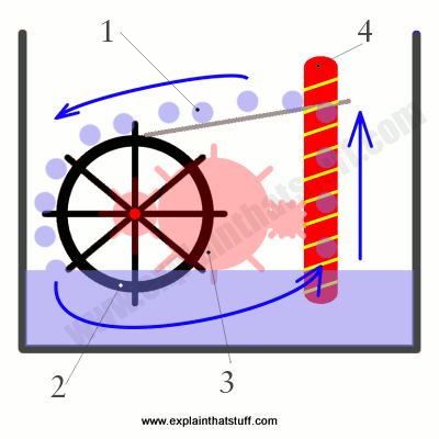
In one version of perpetual motion, illustrated here, water (1) tips down onto a waterwheel, turning
it around (2). The turning wheel drives gears (3) that power an
Archimedes screw,
which lifts the water back up to the top, theoretically allowing the whole cycle to repeat itself
forever. Although you might think energy is being recycled as
the water moves around, it's also being lost all the time. The water
at the top has potential energy and that can indeed drive
a waterwheel as it falls. But some energy will be lost to friction as
the wheel turns. More energy will be lost to friction in the gears and the screw.
So, between them, the wheel, gears, and screw will not have the same
amount of energy as the potential energy the water lost originally.
That means the screw cannot lift as as much water back to the bath as
fell down from it originally—so the machine will very quickly come
to a stop.
What about the conservation of mass?
Nuclear reactions seem to create energy out of nothing breaking up or joining together atoms.
Do they violate the conservation of energy? No!
Albert Einstein's famous equation E=mc
2 shows that energy and mass are
different forms of the same thing. Loosely speaking, you can convert
a small amount of mass into a large amount of energy (as in a
nuclear
power plant, where large
atoms split apart and give off energy in
the process). Einstein's equation shows us we sometimes need to factor
mass into the conservation of energy. In a nuclear reaction, we start
off with one set of atoms (a certain amount of energy in the form of
mass) and end up with a different set of atoms (a different amount of
energy locked in their mass) plus energy that's released as heat. If
we factor in the mass of the atoms before and after the reaction,
plus the energy released in the process, we find the conservation of
energy is satisfied exactly. Since mass is a form of energy, it's
clear that we can't destroy mass or create it out of nothing in the
same way that we can't create or destroy energy.
4
⇉Push vs. pull: data movement for linked data structures⇇
As the performance gap between the CPU and main memory continues
to grow, techniques to hide memory latency are essential to deliver a
high performance computer system. Prefetching can often overlap memory
latency with computation for array-based numeric applications. However,
prefetching for pointer-intensive applications still remains a
challenging problem. Prefetching linked data structures (LDS) is
difficult because the address sequence of LDS traversal does not present
the same arithmetic regularity as array-based applications and the data
dependence of pointer dereferences can serialize the address generation
process.
hardware/software mechanism to reduce memory access latencies for linked
data structures. Instead of relying on the past address history to
predict future accesses, we identify the load instructions that traverse
the LDS, and execute them ahead of the actual computation. To overcome
the serial nature of the LDS address generation, we attach a prefetch
controller to each level of the memory hierarchy and push, rather than
pull, data to the CPU.
Stack (abstract data type)
In
computer science, a
stack is an
abstract data type that serves as a
collection of elements, with two principal operations:
- push, which adds an element to the collection, and
- pop, which removes the most recently added element that was not yet removed.
The order in which elements come off a stack gives rise to its alternative name,
LIFO (
last in, first out). Additionally, a
peek operation may give access to the top without modifying the stack.
The name "stack" for this type of structure comes from the analogy to a
set of physical items stacked on top of each other, which makes it easy
to take an item off the top of the stack, while getting to an item
deeper in the stack may require taking off multiple other items first.
Considered as a
linear data structure,
or more abstractly a sequential collection, the push and pop operations
occur only at one end of the structure, referred to as the
top of the stack. This makes it possible to implement a stack as a
singly linked list
and a pointer to the top element. A stack may be implemented to have a
bounded capacity. If the stack is full and does not contain enough space
to accept an entity to be pushed, the stack is then considered to be in
an
overflow state. The pop operation removes an item from the top of the stack.
A stack is needed to implement
depth-first search.

Similar to a stack of plates, adding or removing is only possible at the top

Simple representation of a stack runtime with
push and
pop operations.
Hardware stack
A common use of stacks at the architecture level is as a means of allocating and accessing memory.
Basic architecture of a stack
A typical stack, storing local data and call information for nested procedure calls (not necessarily
nested procedures). This stack grows downward from its origin. The stack pointer points to the current topmost
datum
on the stack. A push operation decrements the pointer and copies the
data to the stack; a pop operation copies data from the stack and then
increments the pointer. Each procedure called in the program stores
procedure return information (in yellow) and local data (in other
colors) by pushing them onto the stack. This type of stack
implementation is extremely common, but it is vulnerable to
buffer overflow attacks (see the text).
A typical stack is an area of computer memory with a fixed origin and
a variable size. Initially the size of the stack is zero. A
stack pointer,
usually in the form of a hardware register, points to the most recently
referenced location on the stack; when the stack has a size of zero,
the stack pointer points to the origin of the stack.
The two operations applicable to all stacks are:
- a push operation, in which a data item is placed at the
location pointed to by the stack pointer, and the address in the stack
pointer is adjusted by the size of the data item;
- a pop or pull operation: a data item at the current
location pointed to by the stack pointer is removed, and the stack
pointer is adjusted by the size of the data item.
There are many variations on the basic principle of stack operations.
Every stack has a fixed location in memory at which it begins. As data
items are added to the stack, the stack pointer is displaced to
indicate the current extent of the stack, which expands away from the
origin.
Stack pointers may point to the origin of a stack or to a limited
range of addresses either above or below the origin (depending on the
direction in which the stack grows); however, the stack pointer cannot
cross the origin of the stack. In other words, if the origin of the
stack is at address 1000 and the stack grows downwards (towards
addresses 999, 998, and so on), the stack pointer must never be
incremented beyond 1000 (to 1001, 1002, etc.). If a pop operation on
the stack causes the stack pointer to move past the origin of the stack,
a
stack underflow occurs. If a push operation causes the stack pointer to increment or decrement beyond the maximum extent of the stack, a
stack overflow occurs.
Some environments that rely heavily on stacks may provide additional operations, for example:
- Duplicate: the top item is popped, and then pushed again
(twice), so that an additional copy of the former top item is now on
top, with the original below it.
- Peek: the topmost item is inspected (or returned), but the
stack pointer and stack size does not change (meaning the item remains
on the stack). This is also called top operation in many articles.
- Swap or exchange: the two topmost items on the stack exchange places.
- Rotate (or Roll): the n topmost items are moved on the stack in a rotating fashion. For example, if n=3,
items 1, 2, and 3 on the stack are moved to positions 2, 3, and 1 on
the stack, respectively. Many variants of this operation are possible,
with the most common being called left rotate and right rotate.
Stacks are often visualized growing from the bottom up (like
real-world stacks). They may also be visualized growing from left to
right, so that "topmost" becomes "rightmost", or even growing from top
to bottom. The important feature is that the bottom of the stack is in a
fixed position. The illustration in this section is an example of a
top-to-bottom growth visualization: the top (28) is the stack "bottom",
since the stack "top" (9) is where items are pushed or popped from.
A
right rotate will move the first element to the third
position, the second to the first and the third to the second. Here are
two equivalent visualizations of this process:
apple                         banana
banana    ===right rotate==>  cucumber
cucumber                      apple
cucumber                      apple
banana    ===left rotate==>   cucumber
apple                         banana
A stack is usually represented in computers by a block of memory
cells, with the "bottom" at a fixed location, and the stack pointer
holding the address of the current "top" cell in the stack. The top and
bottom terminology are used irrespective of whether the stack actually
grows towards lower memory addresses or towards higher memory addresses.
Pushing an item on to the stack adjusts the stack pointer by the
size of the item (either decrementing or incrementing, depending on the
direction in which the stack grows in memory), pointing it to the next
cell, and copies the new top item to the stack area. Depending again on
the exact implementation, at the end of a push operation, the stack
pointer may point to the next unused location in the stack, or it may
point to the topmost item in the stack. If the stack points to the
current topmost item, the stack pointer will be updated before a new
item is pushed onto the stack; if it points to the next available
location in the stack, it will be updated
after the new item is pushed onto the stack.
Popping the stack is simply the inverse of pushing. The topmost
item in the stack is removed and the stack pointer is updated, in the
opposite order of that used in the push operation.
Stack in main memory
Many
CISC-type
CPU designs, including the
x86,
Z80 and
6502, have a dedicated register for use as the
call stack
stack pointer with dedicated call, return, push, and pop instructions
that implicitly update the dedicated register, thus increasing
code density. Some CISC processors, like the
PDP-11 and the
68000, also have
special addressing modes for implementation of stacks, typically with a semi-dedicated stack pointer as well (such as A7 in the 68000). In contrast, most
RISC
CPU designs do not have dedicated stack instructions and therefore most
if not all registers may be used as stack pointers as needed.
Stack in registers or dedicated memory
The
x87 floating point
architecture is an example of a set of registers organised as a stack
where direct access to individual registers (relative the current top)
is also possible. As with stack-based machines in general, having the
top-of-stack as an implicit argument allows for a small
machine code footprint with a good usage of
bus bandwidth and
code caches, but it also prevents some types of optimizations possible on processors permitting
random access to the
register file for all (two or three) operands. A stack structure also makes
superscalar implementations with
register renaming (for
speculative execution) somewhat more complex to implement, although it is still feasible, as exemplified by modern
x87 implementations.
Sun SPARC,
AMD Am29000, and
Intel i960 are all examples of architectures using
register windows within a register-stack as another strategy to avoid the use of slow main memory for function arguments and return values.
There are also a number of small microprocessors that implements a stack directly in hardware and some
microcontrollers have a fixed-depth stack that is not directly accessible. Examples are the
PIC microcontrollers, the
Computer Cowboys MuP21, the
Harris RTX line, and the
Novix NC4016. Many stack-based microprocessors were used to implement the programming language
Forth at the
microcode level. Stacks were also used as a basis of a number of
mainframes and
mini computers. Such machines were called
stack machines, the most famous being the
Burroughs B5000.
Applications of stacks
Expression evaluation and syntax parsing
Calculators employing
reverse Polish notation
use a stack structure to hold values. Expressions can be represented in
prefix, postfix or infix notations and conversion from one form to
another may be accomplished using a stack. Many compilers use a stack
for parsing the syntax of expressions, program blocks etc. before
translating into low level code. Most programming languages are
context-free languages, allowing them to be parsed with stack based machines.
Backtracking
Another important application of stacks is
backtracking.
Consider a simple example of finding the correct path in a maze. There
are a series of points, from the starting point to the destination. We
start from one point. To reach the final destination, there are several
paths. Suppose we choose a random path. After following a certain path,
we realise that the path we have chosen is wrong. So we need to find a
way by which we can return to the beginning of that path. This can be
done with the use of stacks. With the help of stacks, we remember the
point where we have reached. This is done by pushing that point into the
stack. In case we end up on the wrong path, we can pop the last point
from the stack and thus return to the last point and continue our quest
to find the right path. This is called backtracking.
The prototypical example of a backtracking algorithm is
depth-first search,
which finds all vertices of a graph that can be reached from a
specified starting vertex.
Other applications of backtracking involve searching through spaces that
represent potential solutions to an optimization problem.
Branch and bound
is a technique for performing such backtracking searches without
exhaustively searching all of the potential solutions in such a space.
Compile time memory management
A number of programming languages are stack-oriented,
meaning they define most basic operations (adding two numbers, printing
a character) as taking their arguments from the stack, and placing any
return values back on the stack. For example, PostScript has a return stack and an operand stack, and also has a graphics state stack and a dictionary stack. Many virtual machines are also stack-oriented, including the p-code machine and the Java Virtual Machine.
Almost all calling conventions—the ways in which subroutines receive their parameters and return results—use a special stack (the "call stack")
to hold information about procedure/function calling and nesting in
order to switch to the context of the called function and restore to the
caller function when the calling finishes. The functions follow a
runtime protocol between caller and callee to save arguments and return
value on the stack. Stacks are an important way of supporting nested or recursive
function calls. This type of stack is used implicitly by the compiler
to support CALL and RETURN statements (or their equivalents) and is not
manipulated directly by the programmer.
Some programming languages use the stack to store data that is
local to a procedure. Space for local data items is allocated from the
stack when the procedure is entered, and is deallocated when the
procedure exits. The C programming language
is typically implemented in this way. Using the same stack for both
data and procedure calls has important security implications (see below)
of which a programmer must be aware in order to avoid introducing
serious security bugs into a program.
Efficient algorithms
Several algorithms use a stack (separate from the usual function call stack of most programming languages) as the principle data structure with which they organize their information.
These include:
- Graham scan, an algorithm for the convex hull
of a two-dimensional system of points. A convex hull of a subset of the
input is maintained in a stack, which is used to find and remove
concavities in the boundary when a new point is added to the hull.
- Part of the SMAWK algorithm for finding the row minima of a monotone matrix uses stacks in a similar way to Graham scan.
- All nearest smaller values,
the problem of finding, for each number in an array, the closest
preceding number that is smaller than it. One algorithm for this problem
uses a stack to maintain a collection of candidates for the nearest
smaller value. For each position in the array, the stack is popped until
a smaller value is found on its top, and then the value in the new
position is pushed onto the stack.
- The nearest-neighbor chain algorithm, a method for agglomerative hierarchical clustering
based on maintaining a stack of clusters, each of which is the nearest
neighbor of its predecessor on the stack. When this method finds a pair
of clusters that are mutual nearest neighbors, they are popped and
merged.
Security
Some computing environments use stacks in ways that may make them vulnerable to security breaches and attacks. Programmers working in such environments must take special care to avoid the pitfalls of these implementations.
For example, some programming languages use a common stack to
store both data local to a called procedure and the linking information
that allows the procedure to return to its caller. This means that the
program moves data into and out of the same stack that contains critical
return addresses for the procedure calls. If data is moved to the
wrong location on the stack, or an oversized data item is moved to a
stack location that is not large enough to contain it, return
information for procedure calls may be corrupted, causing the program to
fail.
Malicious parties may attempt a stack smashing
attack that takes advantage of this type of implementation by providing
oversized data input to a program that does not check the length of
input. Such a program may copy the data in its entirety to a location
on the stack, and in so doing it may change the return addresses for
procedures that have called it. An attacker can experiment to find a
specific type of data that can be provided to such a program such that
the return address of the current procedure is reset to point to an area
within the stack itself (and within the data provided by the attacker),
which in turn contains instructions that carry out unauthorized
operations.
This type of attack is a variation on the buffer overflow
attack and is an extremely frequent source of security breaches in
software, mainly because some of the most popular compilers use a shared
stack for both data and procedure calls, and do not verify the length
of data items. Frequently programmers do not write code to verify the
size of data items, either, and when an oversized or undersized data
item is copied to the stack, a security breach may occur.
5
⇉ To operation and change operation in differential mathematics (SET) and integral (RESET)⇇
In
calculus,
Leibniz's rule for differentiation under the integral sign, named after
Gottfried Leibniz, states that for an
integral of the form

where

, the derivative of this integral is expressible as

where the
partial derivative indicates that inside the integral, only the variation of
f(
x,
t) with
x is considered in taking the derivative. Notice that if

and

are constants rather than
functions of

, we have a special case of Leibniz's rule:

- Besides, if
 and
and  , which is a common situation as well (for example, in the proof of Cauchy's repeated integration formula), we have:
Thus under certain conditions, one may interchange the integral and partial differential
operators. This important result is particularly useful in the differentiation of
integral transforms. An example of such is the
moment generating function in
probability theory, a variation of the
Laplace transform, which can be differentiated to generate the
moments of a
random variable. Whether Leibniz's integral rule applies is essentially a question about the interchange of
limits.
General form: Differentiation under the integral sign
- Theorem. Let f(x, t) be a function such that both f(x, t) and its partial derivative fx(x, t) are continuous in t and x in some region of the (x, t)-plane, including a(x) ≤ t ≤ b(x), x0 ≤ x ≤ x1. Also suppose that the functions a(x) and b(x) are both continuous and both have continuous derivatives for x0 ≤ x ≤ x1. Then, for x0 ≤ x ≤ x1,

This formula is the general form of the Leibniz integral rule and can be derived using the
fundamental theorem of calculus. The (first) fundamental theorem of calculus is just the particular case of the above formula where
a(
x) =
a, a constant,
b(
x) =
x, and
f(
x,
t) =
f(
t).
If both upper and lower limits are taken as constants, then the formula takes the shape of an
operator equation:
-

where

is the
partial derivative with respect to
and

is the integral operator with respect to

over a fixed
interval. That is, it is related to the
symmetry of second derivatives, but involving integrals as well as derivatives. This case is also known as the Leibniz integral rule.
The following three basic theorems on the
interchange of limits are essentially equivalent:
- the interchange of a derivative and an integral (differentiation under the integral sign; i.e., Leibniz integral rule);
- the change of order of partial derivatives;
- the change of order of integration (integration under the integral sign; i.e., Fubini's theorem).
Three-dimensional, time-dependent case
Figure 1: A vector field F(r, t) defined throughout space, and a surface Σ bounded by curve ∂Σ moving with velocity v over which the field is integrated.
A Leibniz integral rule for a
two dimensional surface moving in three dimensional space is
![{\displaystyle {\frac {d}{dt}}\iint _{\Sigma (t)}\mathbf {F} (\mathbf {r} ,t)\cdot d\mathbf {A} =\iint _{\Sigma (t)}\left(\mathbf {F} _{t}(\mathbf {r} ,t)+\left[\nabla \cdot \mathbf {F} (\mathbf {r} ,t)\right]\mathbf {v} \right)\cdot d\mathbf {A} -\oint _{\partial \Sigma (t)}\left[\mathbf {v} \times \mathbf {F} (\mathbf {r} ,t)\right]\cdot d\mathbf {s} ,}](https://wikimedia.org/api/rest_v1/media/math/render/svg/78e1920d1765de7da9577a03567e36b3d9d7409e)
where:
- F(r, t) is a vector field at the spatial position r at time t,
- Σ is a surface bounded by the closed curve ∂Σ,
- dA is a vector element of the surface Σ,
- ds is a vector element of the curve ∂Σ,
- v is the velocity of movement of the region Σ,
- ∇⋅ is the vector divergence,
- × is the vector cross product,
- The double integrals are surface integrals over the surface Σ, and the line integral is over the bounding curve ∂Σ.
Higher dimensions
The
Leibniz integral rule can be extended to multidimensional integrals. In
two and three dimensions, this rule is better known from the field of
fluid dynamics as the
Reynolds transport theorem:

where

is a scalar function,
D(
t) and ∂
D(
t) denote a time-varying connected region of
R3 and its boundary, respectively,

is the Eulerian velocity of the boundary (see
Lagrangian and Eulerian coordinates) and
d Σ =
n dS is the unit normal component of the
surface element.
The general statement of the Leibniz integral rule requires concepts from
differential geometry, specifically
differential forms,
exterior derivatives,
wedge products and
interior products. With those tools, the Leibniz integral rule in
n dimensions is
[2]

where Ω(
t) is a time-varying domain of integration, ω is a
p-form,

is the vector field of the velocity,

denotes the
interior product with

,
dxω is the
exterior derivative of ω with respect to the space variables only and

is the time derivative of ω.
However, all of these identities can be derived from a most general statement about Lie derivatives:

Here, the ambient manifold on which the differential form

lives includes both space and time.
 is the region of integration (a submanifold) at a given instant (it does not depend on , since its parametrization as a submanifold defines its position in time),
 is the Lie derivative,
 is the spacetime vector field obtained from adding the unitary vector
field in the direction of time to the purely spatial vector field from the previous formulas (i.e, is the spacetime velocity of ),
is the spacetime vector field obtained from adding the unitary vector
field in the direction of time to the purely spatial vector field from the previous formulas (i.e, is the spacetime velocity of ), is a diffeomorphism from the one-parameter group generated by the flow of , and
 is the image of under such diffeomorphism.
Something remarkable about this form, is that it can account for the case when
changes its shape and size over time, since such deformations are fully determined by
.
Measure theory statement
Let

be an open subset of

, and
be a
measure space. Suppose

satisfies the following conditions:
 is a Lebesgue-integrable function of for each
  .
.- For almost all
 , the derivative
  exists for all .
- There is an integrable function
 such that
  for all and almost every .
Then by the
dominated convergence theorem for all
,

Proofs
Proof of basic form
Let

By the definition of the derivative,

Substitute equation (1) into equation (2). The difference of two integrals equals the integral of the difference, and 1/
h is a constant, so

Provided that the limit can be passed through the integral sign, we obtain

We claim that the passage of the limit under the integral sign is valid by the bounded convergence theorem (a corollary of the
dominated convergence theorem). For each δ > 0, consider the
difference quotient

For
t fixed, the
mean value theorem implies there exists z in the interval [
x,
x + δ] such that

Continuity of
fx(
x,
t) and compactness of the domain together imply that
fx(
x,
t) is bounded. The above application of the mean value theorem therefore gives a uniform (independent of δ) bound on

. The difference quotients converge pointwise to the partial derivative
fx by the assumption that the partial derivative exists.
The above argument shows that for every sequence {δ
n} → 0, the sequence

is uniformly bounded and converges pointwise to
fx.
The bounded convergence theorem states that if a sequence of functions
on a set of finite measure is uniformly bounded and converges
pointwise, then passage of the limit under the integral is valid. In
particular, the limit and integral may be exchanged for every sequence
{δ
n} → 0. Therefore, the limit as δ → 0 may be passed through the integral sign.
For a simpler proof using
Fubini's theorem, see the references.
Variable limits form
For a
continuous real valued function g of one
real variable, and real valued
differentiable functions

and

of one real variable,

This follows from the
chain rule and the
First Fundamental Theorem of Calculus. Define
 ,
,
and
 . (The lower limit just has to be some number in the domain of
  )
)
Then,

can be written as a
composition:

.
The
Chain Rule then implies that
 .
.
By the
First Fundamental Theorem of Calculus,

. Therefore, substituting this result above, we get the desired equation:
 .
.
Note: This form can be particularly useful if the expression to be differentiated is of the form:

Because

does not depend on the limits of integration, it may be move out from
under the integral sign, and the above form may be used with the
Product rule, i.e.

General form with variable limits
Set

where
a and
b are functions of α that exhibit increments Δ
a and Δ
b, respectively, when α is increased by Δα. Then,
![{\displaystyle {\begin{aligned}\Delta \varphi &=\varphi (\alpha +\Delta \alpha )-\varphi (\alpha )\\&=\int _{a+\Delta a}^{b+\Delta b}f(x,\alpha +\Delta \alpha )\,dx-\int _{a}^{b}f(x,\alpha )\,dx\\&=\int _{a+\Delta a}^{a}f(x,\alpha +\Delta \alpha )\,dx+\int _{a}^{b}f(x,\alpha +\Delta \alpha )\,dx+\int _{b}^{b+\Delta b}f(x,\alpha +\Delta \alpha )\,dx-\int _{a}^{b}f(x,\alpha )\,dx\\&=-\int _{a}^{a+\Delta a}f(x,\alpha +\Delta \alpha )\,dx+\int _{a}^{b}[f(x,\alpha +\Delta \alpha )-f(x,\alpha )]\,dx+\int _{b}^{b+\Delta b}f(x,\alpha +\Delta \alpha )\,dx.\end{aligned}}}](https://wikimedia.org/api/rest_v1/media/math/render/svg/0e844395c738c2319ff0faec99332420bafce02d)
A form of the
mean value theorem,

, where
a < ξ <
b, may be applied to the first and last integrals of the formula for Δφ above, resulting in
![{\displaystyle \Delta \varphi =-\Delta af(\xi _{1},\alpha +\Delta \alpha )+\int _{a}^{b}[f(x,\alpha +\Delta \alpha )-f(x,\alpha )]\,dx+\Delta bf(\xi _{2},\alpha +\Delta \alpha ).}](https://wikimedia.org/api/rest_v1/media/math/render/svg/f3e36563c2c4e6f252b197fdf0c03db2e68b869c)
Divide by Δα and let Δα → 0. Notice ξ
1 →
a and ξ
2 →
b. We may pass the limit through the integral sign:

again by the bounded convergence theorem. This yields the general form of the Leibniz integral rule,

Alternative Proof of General Form with Variable Limits, using the Chain Rule
The general form of Leibniz's Integral Rule with variable limits can be derived as a consequence of the
basic form of Leibniz's Integral Rule, the
Multivariable Chain Rule, and the
First Fundamental Theorem of Calculus. Suppose

is defined in a rectangle in the

plane, for
![{\displaystyle x\in [x_{1},x_{2}]}](https://wikimedia.org/api/rest_v1/media/math/render/svg/28267d22f13c327a49b44a9cb3f3e4cd38b39d13)
and
![{\displaystyle t\in [t_{1},t_{2}]}](https://wikimedia.org/api/rest_v1/media/math/render/svg/e3e34a2927bca2a13a30ae0e6fc3a757366e0ba6)
. Also, assume
and the partial derivative

are both continuous functions on this rectangle. Suppose

are
differentiable real valued functions defined on
![{\displaystyle [x_{1},x_{2}]}](https://wikimedia.org/api/rest_v1/media/math/render/svg/91bdff343d848c2b70c68b5c04a2479b14a9fef0)
, with values in
![{\displaystyle [t_{1},t_{2}]}](https://wikimedia.org/api/rest_v1/media/math/render/svg/6e35e13fa8221f864808f15cafa3d1467b5d78ce)
(i.e. for every
![{\displaystyle x\in [x_{1},x_{2}],a(x),b(x)\in [t_{1},t_{2}]}](https://wikimedia.org/api/rest_v1/media/math/render/svg/5c47e98fcb040ce05754e1e93c3342f483b47d5e)
). Now, set
 , for and
 ![{\displaystyle y\in [t_{1},t_{2}]}](https://wikimedia.org/api/rest_v1/media/math/render/svg/2b3dbc62b50259c75e078c02fbf9d36176b69611)
and
 , for
, for
Then, by properties of
Definite Integrals, we can write

Since the functions

are all differentiable (see the remark at the end of the proof), by the
Multivariable Chain Rule, it follows that

is differentiable, and its derivative is given by the formula:

Now, note that for every
, and for every
, we have that

, because when taking the partial derivative with respect to
of

, we are keeping

fixed in the expression

; thus the
basic form of Leibniz's Integral Rule with constant limits of integration applies. Next, by the
First Fundamental Theorem of Calculus, we have that

; because when taking the partial derivative with respect to
of
, the first variable
is fixed, so the fundamental theorem can indeed be applied.
Substituting these results into the equation for

above gives:

as desired.
There is a technical point in the proof above which is worth noting: applying the Chain Rule to
requires that
already be
Differentiable. This is where we use our assumptions about
. As mentioned above, the partial derivatives of
are given by the formulas
and
. Since
is continuous, its integral is also a continuous function, and since
is also continuous, these two results show that both the partial derivatives of
are continuous. Since continuity of partial derivatives implies differentiability of the function,
is indeed differentiable.
Three-dimensional, time-dependent form
At time
t the surface Σ in
Figure 1 contains a set of points arranged about a centroid

. The function

can be written as

with

independent of time. Variables are shifted to a new frame of reference attached to the moving surface, with origin at
. For a rigidly translating surface, the limits of integration are then independent of time, so:

where the limits of integration confining the integral to the region Σ
no longer are time dependent so differentiation passes through the
integration to act on the integrand only:

with the velocity of motion of the surface defined by

This equation expresses the
material derivative
of the field, that is, the derivative with respect to a coordinate
system attached to the moving surface. Having found the derivative,
variables can be switched back to the original frame of reference. We
notice that (see
article on curl)

and that
Stokes theorem equates the surface integral of the curl over Σ with a line integral over ∂Σ:

The sign of the line integral is based on the
right-hand rule for the choice of direction of line element
ds. To establish this sign, for example, suppose the field
F points in the positive
z-direction, and the surface Σ is a portion of the
xy-plane with perimeter ∂Σ. We adopt the normal to Σ to be in the positive
z-direction. Positive traversal of ∂Σ is then counterclockwise (right-hand rule with thumb along
z-axis). Then the integral on the left-hand side determines a
positive flux of
F through Σ. Suppose Σ translates in the positive
x-direction at velocity
v. An element of the boundary of Σ parallel to the
y-axis, say
ds, sweeps out an area
vt ×
ds in time
t. If we integrate around the boundary ∂Σ in a counterclockwise sense,
vt ×
ds points in the negative
z-direction on the left side of ∂Σ (where
ds points downward), and in the positive
z-direction on the right side of ∂Σ (where
ds
points upward), which makes sense because Σ is moving to the right,
adding area on the right and losing it on the left. On that basis, the
flux of
F is increasing on the right of ∂Σ and decreasing on the left. However, the dot product
v ×
F • ds = −
F ×
v •
ds = −
F • v ×
ds. Consequently, the sign of the line integral is taken as negative.
If
v is a constant,

which is the quoted result. This proof does not consider the possibility of the surface deforming as it moves.
Alternative derivation
Lemma. One has:

Proof. From
proof of the fundamental theorem of calculus,
![{\displaystyle {\begin{aligned}{\frac {\partial }{\partial b}}\left(\int _{a}^{b}f(x)\,dx\right)&=\lim _{\Delta b\to 0}{\frac {1}{\Delta b}}\left[\int _{a}^{b+\Delta b}f(x)\,dx-\int _{a}^{b}f(x)\,dx\right]\\&=\lim _{\Delta b\to 0}{\frac {1}{\Delta b}}\int _{b}^{b+\Delta b}f(x)\,dx\\&=\lim _{\Delta b\to 0}{\frac {1}{\Delta b}}\left[f(b)\Delta b+O\left(\Delta b^{2}\right)\right]\\&=f(b),\end{aligned}}}](https://wikimedia.org/api/rest_v1/media/math/render/svg/d8cc613cf0ffb14b36116c6b713274f4606723c8)
and
![{\displaystyle {\begin{aligned}{\frac {\partial }{\partial a}}\left(\int _{a}^{b}f(x)\,dx\right)&=\lim _{\Delta a\to 0}{\frac {1}{\Delta a}}\left[\int _{a+\Delta a}^{b}f(x)\,dx-\int _{a}^{b}f(x)\,dx\right]\\&=\lim _{\Delta a\to 0}{\frac {1}{\Delta a}}\int _{a+\Delta a}^{a}f(x)\,dx\\&=\lim _{\Delta a\to 0}{\frac {1}{\Delta a}}\left[-f(a)\Delta a+O\left(\Delta a^{2}\right)\right]\\&=-f(a).\end{aligned}}}](https://wikimedia.org/api/rest_v1/media/math/render/svg/ec95fceffc789ee8cb714bee89fb8232cdccd47b)
Suppose
a and
b are constant, and that
f(
x) involves a parameter α which is constant in the integration but may vary to form different integrals. Assume that
f(
x, α) is a continuous function of
x and α in the compact set {(
x, α) : α
0 ≤ α ≤ α
1 and
a ≤
x ≤
b}, and that the partial derivative
fα(
x, α) exists and is continuous. If one defines:
then

may be differentiated with respect to α by differentiating under the integral sign, i.e.,

By the
Heine–Cantor theorem it is uniformly continuous in that set. In other words, for any ε > 0 there exists Δα such that for all values of
x in [
a,
b],

On the other hand,

Hence φ(α) is a continuous function.
Similarly if

exists and is continuous, then for all ε > 0 there exists Δα such that:
![{\displaystyle \forall x\in [a,b],\quad \left|{\frac {f(x,\alpha +\Delta \alpha )-f(x,\alpha )}{\Delta \alpha }}-{\frac {\partial f}{\partial \alpha }}\right|<\varepsilon .}](https://wikimedia.org/api/rest_v1/media/math/render/svg/b3c46cc29cd17e5bba84da7e4b546591b803820c)
Therefore,

where

Now, ε → 0 as Δα → 0, so

This is the formula we set out to prove.
Now, suppose

where
a and
b are functions of α which take increments Δ
a and Δ
b, respectively, when α is increased by Δα. Then,
A form of the
mean value theorem,

where
a < ξ <
b, can be applied to the first and last integrals of the formula for Δφ above, resulting in
![{\displaystyle \Delta \varphi =-\Delta a\,f(\xi _{1},\alpha +\Delta \alpha )+\int _{a}^{b}[f(x,\alpha +\Delta \alpha )-f(x,\alpha )]\,dx+\Delta b\,f(\xi _{2},\alpha +\Delta \alpha ).}](https://wikimedia.org/api/rest_v1/media/math/render/svg/81c03a4ea6d77c7f3f621471c4d7b1522e9da0f3)
Dividing by Δα, letting Δα → 0, noticing ξ
1 →
a and ξ
2 →
b and using the above derivation for

yields

This is the general form of the Leibniz integral rule.
Examples
General examples
Example 1
Consider the function

The function under the integral sign is not continuous at the point (
x, α) = (0, 0), and the function φ(α) has a discontinuity at α = 0 because φ(α) approaches ±π/2 as α → 0
±.
If we differentiate φ(α) with respect to α under the integral sign, we get

which is, of course, true for all values of α except α = 0. This may be integrated (with respect to α) to find

Example 2
An example with variable limits:

Examples for evaluating a definite integral
Example 3
The principle of differentiating under the integral sign may sometimes be used to evaluate a definite integral. Consider:

Now,

As
x varies from 0 to π, we have

Hence,

Therefore,

Integrating both sides with respect to
α, we get:

C1 = 0 follows from evaluating
φ(0):

To determine
C2 in the same manner, we should need
to substitute in a value of α greater than 1 in φ(α). This is somewhat
inconvenient. Instead, we substitute α = 1/β, where |β| < 1. Then,

Therefore,
C2 = 0.
The definition of
φ(α) is now complete:

The foregoing discussion, of course, does not apply when
α = ±1, since the conditions for differentiability are not met.
Example 4

First we calculate:

The limits of integration being independent of
a, we have:

On the other hand:

Equating these two relations then yields

In a similar fashion, pursuing

yields

Adding the two results then produces

which computes

as desired.
This derivation may be generalized. Note that if we define

it can easily be shown that

Given
I1, this integral reduction formula can be used to compute all of the values of
In for
n > 1.
Example 5
Here, we consider the integral

Differentiating under the integral with respect to α, we have

Therefore:

However, by definition,
I(π/2) = 0, hence
C = π
2/8 and

Example 6
Here, we consider the integral

We introduce a new variable φ and rewrite the integral as

When φ = 1 this equals the original integral. However, this more general integral may be differentiated with respect to φ:

This is the line integral of

over the unit circle. By Green's Theorem, it equals the double integral over the unit disk of

which equals 0. This implies that
f(φ) is constant. The constant may be determined by evaluating
f at φ = 0:

Therefore, the original integral also equals 2π.
Other problems to solve
There
are innumerable other integrals that can be solved using the technique
of differentiation under the integral sign. For example, in each of the
following cases, the original integral may be replaced by a similar
integral having a new parameter α:

The first integral, the
Dirichlet integral,
is absolutely convergent for positive α but only conditionally
convergent when α is 0. Therefore, differentiation under the integral
sign is easy to justify when α > 0, but proving that the resulting
formula remains valid when α is 0 requires some careful work.
Applications to series
The
measure-theoretic version of differentiation under the integral sign
also applies to summation (finite or infinite) by interpreting summation
as
counting measure. An example of an application is the fact that power series are differentiable in their radius of convergence.
In popular culture
Differentiation under the integral sign is mentioned in the late
physicist Richard Feynman's best-selling memoir
Surely You're Joking, Mr. Feynman! in the chapter "A Different Box of Tools". He describes learning it, while in
high school, from an old text,
Advanced Calculus (1926), by
Frederick S. Woods (who was a professor of mathematics in the
Massachusetts Institute of Technology). The technique was not often taught when Feynman later received his formal education in
calculus,
but using this technique, Feynman was able to solve otherwise difficult
integration problems upon his arrival at graduate school at
Princeton University:
One thing I never did learn was contour integration.
I had learned to do integrals by various methods shown in a book that
my high school physics teacher Mr. Bader had given me. One day he told
me to stay after class. "Feynman," he said, "you talk too much and you
make too much noise. I know why. You're bored. So I'm going to give you a
book. You go up there in the back, in the corner, and study this book,
and when you know everything that's in this book, you can talk again."
So every physics class, I paid no attention to what was going on with
Pascal's Law, or whatever they were doing. I was up in the back with
this book: "Advanced Calculus", by Woods. Bader knew I had studied "Calculus for the Practical Man" a little bit, so he gave me the real works—it was for a junior or senior course in college. It had Fourier series, Bessel functions, determinants, elliptic functions—all
kinds of wonderful stuff that I didn't know anything about. That book
also showed how to differentiate parameters under the integral sign—it's
a certain operation. It turns out that's not taught very much in the
universities; they don't emphasize it. But I caught on how to use that
method, and I used that one damn tool again and again. So because I was
self-taught using that book, I had peculiar methods of doing integrals.
The result was, when guys at MIT or Princeton
had trouble doing a certain integral, it was because they couldn't do
it with the standard methods they had learned in school. If it was
contour integration, they would have found it; if it was a simple series
expansion, they would have found it. Then I come along and try
differentiating under the integral sign, and often it worked. .
6
⇉ SPACE AND TIME on PUSH AND PULL ⇇
Both push and pull drive our galaxy's race through space
Discovery of the 'dipole repeller' confirms that both attraction and repulsion are at play in our extragalactic neighborhood
Although we can't feel it, we're in constant
motion: the earth spins on its axis at about 1,600 km/h; it orbits
around the sun at about 100,000 km/h; the sun orbits our Milky Way
galaxy at about 850,000 km/h; and the Milky Way galaxy and its companion
galaxy Andromeda are moving with respect to the expanding universe at
roughly 2 million km/h (630 km per second). But what is propelling the
Milky Way's race through space?
Until now, scientists assumed that a dense region of the universe is
pulling us toward it, in the same way that gravity made Newton's apple
fall to earth. The initial "prime suspect" was called the Great
Attractor, a region of a half dozen rich clusters of galaxies 150
million lightyears from the Milky Way. Soon after, attention was drawn
to an area of more than two dozen rich clusters, called the Shapley
Concentration, which sits 600 million lightyears beyond the Great
Attractor.
By identifying the Dipole Repeller, the researchers were able to
reconcile both the direction of the Milky Way's motion and its
magnitude. They expect that future ultra-sensitive surveys at optical,
near-infrared and radio wavelengths will directly identify the few
galaxies expected to lie in this void, and directly confirm the void
associated with the Dipole Repeller.
Earth is a time space dimension, so it operates in a way that what fills the space then creates either distance or nearness, a longer time or a shorter time.
Congruence is an amazing word, when you allow the vibration of it to truly sink in. It describes a situation where in the moment (time), you are filling your cells and being with a message that all parts of you is agreeing on (space). If you understand this, then understand that everything that occurs as a response to you, offers you a mirror. For example, you’re a full yes to something, and then you present the idea to someone else and they’re a full no. Do you still remain a full yes? Or do you see it for what it is, you are in congrunece in this moment, and they are not? Do you use this as an opportunity to sharpen your articulation, so they are able to get a clear idea of just how congruent you are? Or do you slink away wounded, contracted and caved in? In response to a no do you strengthen your yes, so that you’re not just in agreement you are also amplified?
If even a small part of you is out of alignment with the rest of you, then over time it will make itself known. That small part will convince you that it’s there to look after your best interest and keep you safe. You can consider it to be your gate keeper of sorts, it wants you to put your money where your mouth is. It will niggle, and niggle, and niggle, and niggle, in a quest for you to make the same decision over, and over, and over, and over. Eventually when enough of you is amplified you’ll have pulled the keeper to your side, the gate opens and this becomes your new way of being. Instantly you feel the change because the world begins to respond very differently to you. That part of your life gets easier, just for a little while.
So pay attention to the areas where you’re broadcasting and amplifying a push pull type of energy. Sending mixed messages into the universe, also making it such that you’re not amplifed enough to become magnetic. You stengthen, then weaken, then weaken, then weaken, then strengthen. The energy is counter productive. Empower your stance, empower your decision and empower your actions.
+++++++++++++++++++++++++++++++++++++++++++++++++++++++++++++++++++
Gen . Mac Tech in operation to change operation
+++++++++++++++++++++++++++++++++++++++++++++++++++++++++++++++++++++++


_Switch_State_S1_b)_Switch_State_S3_c)_S1_Output_d)_S3_Output.jpg)

_Carrier_and_Modulating_Signals_b)_S1_State_c)_S3_State_d)_Output_Current.jpg)