
we can explain the basic principles of electronic solenoid valve in the electronic circuit of the pool water pump as follows:
simple circuit and working principle of an electronic pump both an air pump and a liquid made by an electronic circuit from a simple adapter that is a transformer that uses an iron core and one part of the iron core that is left open to attract and emit electromagnetic waves where the waves magnetic electronics emit and receive vibrations that pull the air pump lever with certain vibrations that can be regulated through capacitor and parallelized resistors after the electromagnetic transformer circuit so that after the lever moves up and down like we are stepping on the car's gas pedal continuously with a certain frequency then making air media pumped and interested in causing airwaves and grains of water in artificial ponds or lakes that we want to make the subject of maintaining living things such as fish and other aquatic ecosystems.
LOVE ( Line On Victory Endless ) with ADAPTER
( Allow Difference Application To Rest Ability )

Gen . Mac Tech Zone Electronic For Rest Up
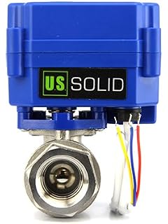
Solenoids of all different sizes are used in most electro-mechanical systems. Because solenoids are so prolific, there are also many different ways to drive them. These methods include several off the shelf options such as PWM chips, mechanical relays, and alternate circuit designs.
Basic Transistor / Fast Response
This circuit schematic demonstrates the simplest form of solenoid drive circuitry and may be used to actuate most solenoid operated valves and pumps .
The circuit requires an input voltage (Vcc) to actuate the solenoid as well as a control signal input (from a controller, function generator, or timing circuit), which switches a transistor. This, in turn, allows the drive current to energize the solenoid. A diode is placed in parallel with the solenoid to protect the transistor from the inductive voltage spike which occurs as the solenoid de-energizes. A significant voltage drop between the power supply and solenoid may occur if there is unexpected resistance, such as long lead wires or other electrical components. Therefore, be sure to verify that the solenoid is receiving its rated actuation voltage by measuring directly across the solenoid's pins. Depending on your application requirements, this circuit may be configured for two different operating modes:
- Basic Driver – In the simplest operating mode, this most basic solenoid drive schematic does not require the 51V Zener diode.
- Fast Response Driver – A 51V Zener diode placed in series with a flyback protection diode improves the latch-out response (time to close) of the solenoid when power is removed.
Basic Transistor Circuit Schematic
Spike & Hold
This circuit can be used as either an enhanced response time driver or as a low power consumption driver. The circuit initially supplies a brief actuation voltage (V1, “Spike” Voltage), for a period of time (ts), then switches to a lower voltage (V2, “Hold” Voltage), to keep the solenoid in an energized state for an extended time. The duration of the spike (ts) is determined by a resistor and capacitor (R1 and C1 indicated on LFIX1002250A, Note 4), connected to a 555 timer chip. Typically, the spike duration is slightly longer than the response time of the solenoid. A control signal input is required (from a controller, function generator, or timing circuit), to actuate the solenoid. The solenoid will remain actuated for as long as the control signal is applied. A significant voltage drop between the power supply and solenoid may occur if there is unexpected resistance, such as long lead wires or other electrical components. Therefore, be sure to verify that the solenoid is receiving its rated actuation voltage by measuring directly across the solenoid's pins. When measuring the signal between the solenoid pins with an oscilloscope, ensure that a differential probe is used.
Depending on whether you require lower power or faster response, this driver may be configured for two different operating modes:
- Fast response spike & hold driver – Solenoid response time can be improved for both actuation (time to open), and latch-out (time to close), of the solenoid by applying an “over-drive” voltage greater than the rated actuation voltage to V1, and adding a 51V Zener Diode (D4, indicated on LFIX1002250A, Note 5.1). After quickly actuating the solenoid, the driver switches to a lower holding voltage applied at V2 to reduce resistive heating and avoid damage to the solenoid. A 51V Zener diode placed in series with a flyback protection diode improves the latch-out response (time to close) of the solenoid when power is removed.
- Low power consumption driver – Overall power consumption can be significantly reduced (typically 75-90%), by applying the rated solenoid voltage to V1, and a lower hold voltage to V2. For most solenoids the hold voltage is half of the rated actuation voltage, unless otherwise indicated on the inspection drawing.
Spike & Hold Circuit Schematic

Circuit Schematic
The primary advantage of a latching solenoid valve is that power is not required to maintain the valve’s flow state (either open or closed) between actuations. That is, a de-energized latching valve will hold its current flow state. Because of this magnetically latched feature, latching solenoid valves have polarized leads which require a different type of drive circuitry. The flow state of the solenoid is determined by a negative or positive voltage pulse, so a circuit capable of bi-directional current flow is required. The recommended LFIX1002350A schematic includes an H-bridge chip which reverses the direction of current flow, allowing for effective latching solenoid valve switching. A significant voltage drop between the power supply and solenoid may occur if there is unexpected resistance, such as long lead wires or other electrical components. Therefore, be sure to verify that the solenoid is receiving its rated actuation voltage by measuring directly across the solenoid's pins.
This schematic requires the rated input voltage to actuate the solenoid as well as switching commands provided by a micro-controller (MCU), or other programmable logic controller (PLC). Switching commands should be provided as a 5 Vdc “HIGH” or “LOW” signal, of which four are required. Two pins are required to enable the H-bridge chip, and two others are required to trigger either a positive or negative pulse to the solenoid. A description of each pin is included below, along with a state diagram. Information about solenoid pin assignments and the porting arrangements can be found on the inspection drawing for each latching solenoid valve.
MCU Pin Assignments (Waveform Graph)
- IN1 – HIGH provides a +5 Vdc pulse. The pulse length (time) should be slightly longer than response time of the solenoid.
- IN2 – HIGH provides a -5 Vdc pulse. The pulse length (time) should be slightly longer than response time of the solenoid.
- D1 - Enables NXP33886 (H-Bridge Chip), should be HIGH when actuating (in either direction).
- D2 - Enables NXP33886 (H-Bridge Chip), should be LOW when actuating (in either direction).
Latching Valve Circuit Schematic

Waveform Graph

Simple Efficient
Solenoid Driver
Solenoid loads generally exhibit large hysteresis. Application
of the rated voltage actuates these loads. Once they are in position, however,
you can use a significantly lower voltage to thereafter reliably hold them on.
A lower sustaining voltage results in less heat production and higher
efficiency.
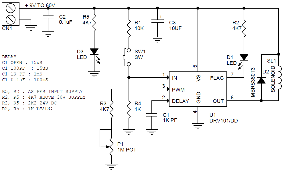
The DRV101 is a low-side power switch employing a pulse-width modulated (PWM) output. Its rugged design is optimized for driving electromechanical devices such as valves, solenoids, relays, actuators, and positioners. The DRV101 module is also ideal for driving thermal devices such as heaters and lamps. PWM operation conserves power and reduces heat rise, resulting in higher reliability. In addition, adjustable PWM potentiometer allows fine control of the power delivered to the load. Time from dc output to PWM output is externally adjustable. The DRV101 can be set to provide a strong initial closure, automatically switching to a soft hold mode for power savings. Duty cycle can be controlled by a potentiometer, analog voltage, or digital-to-analog converter for versatility. A flag output LED D2 indicates thermal shutdown and over/under current limit. A wide supply range allows use with a variety of actuators.
FEATURES
- HIGH OUTPUT DRIVE: 2.3A
- WIDE SUPPLY RANGE: +9V to +60V
- COMPLETE FUNCTION
- PWM Output
- Internal 24 kHz Oscillator
- Digital Control Input
- Adjustable Delay (Capacitor C1)
- Adjustable Duty Cycle P1 Potentiometer
- Over/Under Current Indicator
- FULLY PROTECTED
- Thermal Shutdown with Indicator
- Internal Current Limit
APPLICATIONS
- ELECTROMECHANICAL DRIVERS:
- Solenoids Positioners
- Actuators High Power Relays/Contactors
- Valves Clutch/Brake
- FLUID AND GAS FLOW SYSTEMS
- INDUSTRIAL CONTROL
- FACTORY AUTOMATION
- PART HANDLERS
- PHOTOGRAPHIC PROCESSING
- ELECTRICAL HEATERS
- MOTOR SPEED CONTROL
- SOLENOID/COIL PROTECTORS
- MEDICAL ANALYZERS
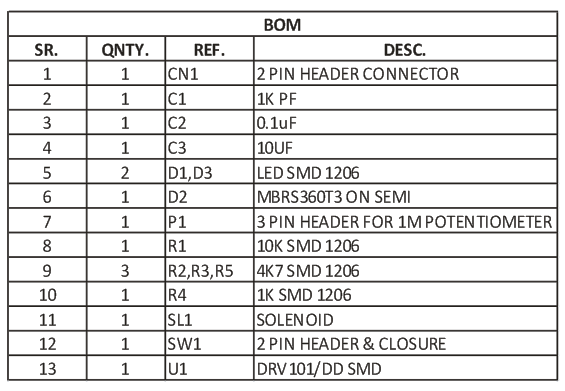
PARTS LIST
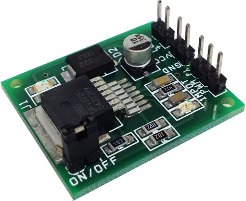
PHOTOS
PCB

AB . WXO PUMP ON PASSING MECHANIC
Materials
Pumps and their various components are made up of a number of
different materials. Media type, system requirements, and the surrounding
environment all are important factors in material selection.
Types
Some materials used are described below.
·
Cast iron provides high tensile strength,
durability, and abrasion resistance corresponding to high pressure
ratings.
·
Plastics are inexpensive and provide extensive
resistance to corrosion and chemical attack.
·
Steel and stainless steel alloys provide
protection against chemical and rust corrosion and have higher tensile
strengths than plastics, corresponding to higher pressure ratings.
Other materials used in pump construction include:
·
Aluminum
·
Brass
·
Bronze
·
Ceramics
·
Nickel-alloy
Considerations
When selecting the material type, there are a number of
considerations that need to be taken into account.
·
Chemical compatibility - Pump parts in contact with
the pumped media and addition additives (cleaners, thinning solutions) should
be made of chemically compatible materials that will not result in
excessive corrosion or contamination. Consult a metallurgist for proper metal
selection when dealing with corrosive media.
·
Explosion proof - Non-sparking materials
are required for operating environments or media with particular susceptibility
to catching fire or explosion.
·
Sanitation- Pumps in the food and beverage
industries require high density seals or sealless pumps that are easy to clean
and sterilize.
·
Wear - Pumps which handle abrasives
require materials with good wearing capabilities. Hard surfaces and chemically
resistant materials are often incompatible. The base and
housing materials should be of adequate strength and also be able
to hold up against the conditions of its operating environment.
Media Type
Selecting the right pump requires an understanding of the
properties of the liquid in the addressed system. These properties include
viscosity and consistency.
·
Viscosity is a measure of the thickness
of a liquid. Viscous fluids like sludges generate higher systems pressures and
require more pumping powerto move through the system. Low viscosity liquids
like water and oil which generate low head. Axial flow pumps are designed to
handle low viscosity fluids because they generate low head and high capacities.
·
Consistency is the material makeup of the liquid solution in terms of
chemicals and undissolved solids. Axial flow pumps are not well-suited for
handling media with solids, but can be used when designed with the proper
impeller type. Solutions with corrosive chemicals should be handled by pumps
with materials and parts designed to withstand corrosion.
Applications
Axial flow pumps are used in applications requiring very high
flow rates and low pressures. They are used to circulate fluids in power
plants, sewage digesters, and evaporators. They are also used in
flood dewatering and irrigation systems. The applications for axial flow
pumps are not nearly as abundant however as for radial flow pumps, so the
equipment is not as common.
When selecting an axial flow pump, there are a few key
performance specifications to consider:
·
Flow rate describes the rate at which the pump
can move fluid through the system, typically expressed in gallons per minute
(gpm). The rated capacity of a pump must be matched to the flow rate required
by the application or system.
·
Pressure is a measure of the force per
unit area of resistance the pump can handle or overcome, expressed in bar
or psi (pounds per square inch). As in all centrifugal pumps, the pressure in
axial flow pumps varies based on the pumped fluid's specific gravity. For this
reason, head is more commonly used to define pump energy in this way.
·
Head is the height above the suction inlet that a
pump can lift a fluid. It is a shortcut measurement of system resistance
(pressure) which is independent of the fluid's specific gravity, expressed
as a column height of water given in feet (ft) or meters (m).
·
Net positive suction head (NPSH) is
the difference between the pump's inlet stagnation pressure head and the vapor
pressure head. The required NPSH is an important parameter
in preventing pump cavitation.
·
Output power, also called water horsepower, is
the power actually delivered to the fluid by the pump, measured in horsepower
(hp).
·
Input power, also called brake horsepower, is
the power that must be supplied to the pump, measured in horsepower (hp).
Efficiency is the ratio between the input power and
output power. It accounts for energy losses in the pump (friction and slip) to
describes how much of the input power does useful work .
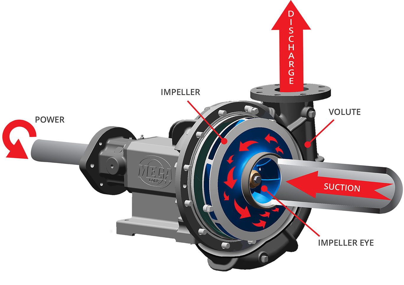
What is an open centrifugal pump?
Centrifugal water pumps use centrifugal force to pressurize and move water from the inlet to the outlet. A rotating set of vanes (called an 'impeller') is spun by the pump shaft. As water is forced through the impeller, rotational energy is transferred from the impeller to the water, which gains velocity and pressure through the centrifugal force applied and is flung from the impeller. The volute (a spiral-shaped case) funnels the now-pressurized water to the outlet. Image below shows clockwise rotation as viewed from the motor mound.
Pressure and Flow, and what causes water pressure.
Pressure and flow are inversely related–that is, if pressure is increased, then flow decreases, and vice versa. "Pressure" is the amount of force per area, and "flow" is the volume of material moving through a given area per second (not the same as velocity, which is the distance traveled per time).
Water pressure is caused by resistance to flow. If a force tries to move water and there is resistance to that movement, then the water becomes pressurized. Consider a standard garden hose; when the end of the hose is unrestricted, water flows out of the hose in large quantities, but without much force. If you press your thumb over the opening, however, the stream of water that shoots out from around your thumb will be much more forceful and will travel further, but there will also be less water per second leaving the hose.
What happens when an open centrifugal pump is "Dead-headed"?
A centrifugal pump is 'dead-headed' when it is operated without an open discharge outlet. Contrary to what one might assume, centrifugal pumps cannot be stalled if water flow is cut off. Very little horsepower input is required in order to spin the impeller with no water flow, so if the pump is driven by a hydraulic motor, the input hydraulic pressure will be low and the pump will not stall, instead continuing to spin the same volume of water as it would during normal operation. With no outlet, the rotational energy of the shaft and impeller is converted into heat; eventually, the water will boil inside the volute, causing severe damage over time.
When should I replace gaskets?
Any time that the water pump is serviced and the gaskets are removed, replace the gaskets. Gaskets are inexpensive, and a faulty gasket will cause the pump to leak.
How do I adjust the packing, and when should I adjust it?
Different types of packing are designed to leak at certain rates. If the packing begins to leak at a greater rate than the allowed amount, tighten the packing gland with a simple end wrench until the leakage is reduced to lie within the packing parameters. Additionally, the stuffing box temperature should be checked regularly. If the temperature becomes too high, loosen the packing gland until the temperature drops to a consistently safe level.
When should I replace the packing?
Over time as the packing is subjected to continual heat and pressure through normal use, lubricant will be forced out of the packing material. The life of the packing material can be extended by periodically tightening the packing gland whenever there is packing leakage greater than the specified amount (Mega's rope packing seals are designed to leak approximately 60 drops per minute). Eventually, however, all of the lubricant will have been squeezed out of the packing material, and tightening the packing gland will no longer prevent leakage. When this happens, it is time to replace the packing.
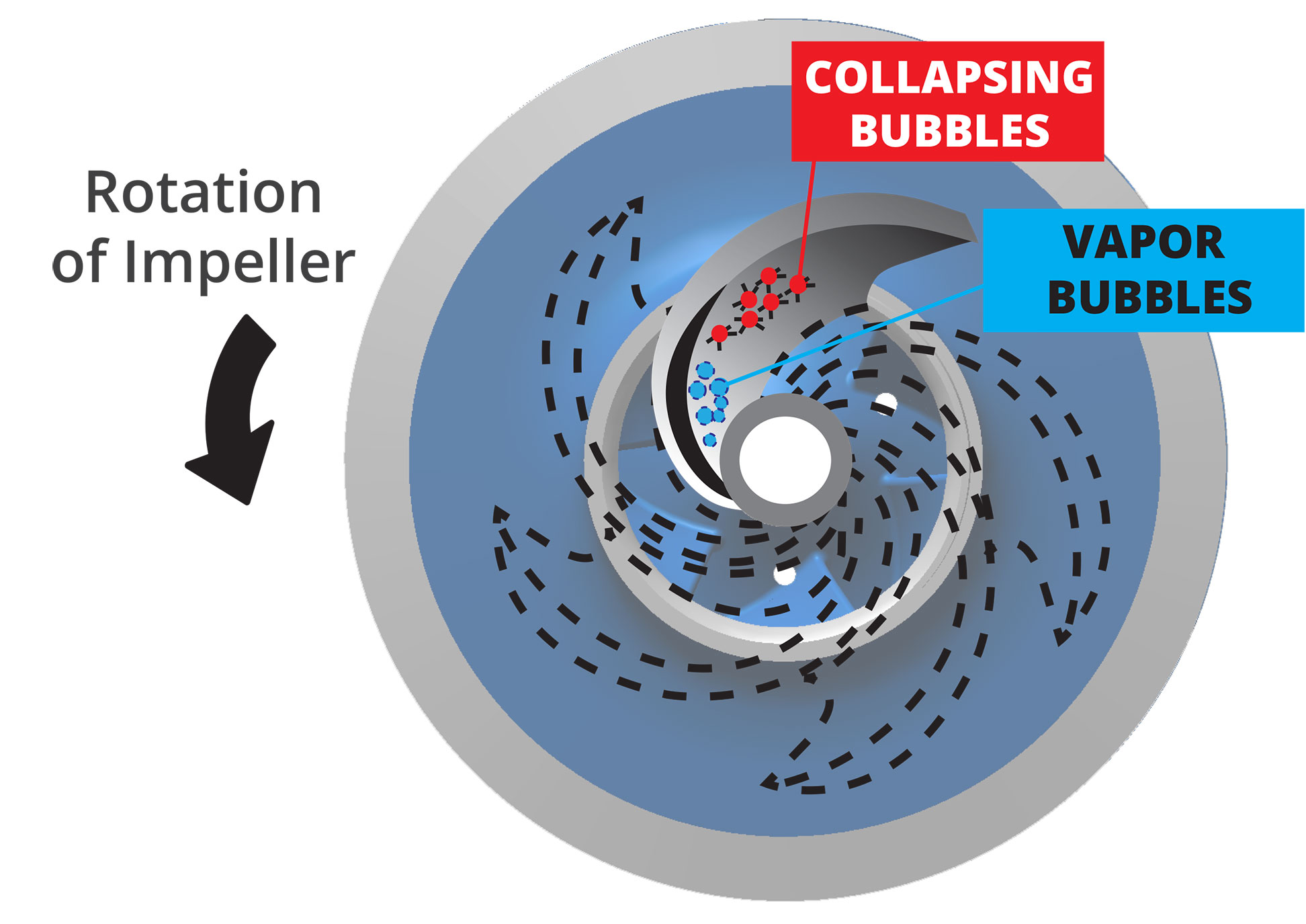
What causes pump cavitation?
When the inlet pressure of a water pump falls below pump design specifications, tiny vapor bubbles can form in the water around the eye of the impeller. When the water containing these bubbles is forced into a high pressure environment on the other side of the impeller, these bubbles collapse, thereby creating tiny shock waves and points of high temperature. These shock waves can actually corrode the surface of the impeller. To prevent cavitation, always be sure to operate your water pump within its pressure and flow specifications.
Is it bad to run the pump dry?
Absolutely. The water pump shaft and impeller are spinning at extremely fast rates. With no water to transfer their rotational energy to, that energy is released as heat instead. If the pump is run dry, its moving parts will become extremely hot, causing severe damage to the pump over time and greatly limiting its service life.
Will this pump pull water up vertically?
MG Corp. offers one self-priming centrifugal pump for suction lifting applications: the B4-Z. This pump can lift water a vertical distance of 7-10 feet.
Why is my spray performance low?
Several factors can affect water pump performance. If low water output is noticed, one of the first things to check is the water pump shaft rpm to ensure it is spinning within specifications. Also check that the water inlet of the pump is not obstructed. Also check to see if the impeller is damaged or if the shaft bearings are worn or damaged.
Why isn't my pump pumping?
There could be several factors behind this:
- Is there enough water? Check to ensure that there is enough water present in the tank to allow safe pumping; the Mega Digital Spray Control System shuts the water pump once a sufficiently low water level has been reached.
- Beware of air locks. If there is too little water in the tank, the pump may have drawn in a large air pocket that is preventing the flow of water (see What is an air lock? question below).
- Is the lift displacement too great? If you are operating a suction lift pump, be sure that the water reservoir you are drawing from is no more than 7 feet below the pump, otherwise the resistance to flow may be too great.
- Are you using pipes that are too small or have too many elbows? Pumping water through small diameter pipes (and pipes with elbows and check valves) increases the water pressure, but as a result also increases flow resistance. If the resistance is too great, your pump will not perform.
What is an air lock?
An air lock occurs when large pockets of air are drawn into the inlet side of the water pump. This essentially acts as a void, and can prevent the pump from drawing in water. Not only will this decrease (or even stop) pump performance, it can be very damaging as well. If the air pocket is drawn through the impeller and into an area of high water pressure, the bubbles will collapse and create large shock waves that will severely damage the pump.
Why did the pump shaft break?
Water pump shaft failures can be caused by several factors:
- Sudden start or stop of the pump.
- Pump rpm should be ramped up and down over a minimum of 2 seconds.
- Engaging a water pump suddenly can twist the impeller off the shaft and damage shaft bearings.
- Water hammer caused by sudden shut off of water flow can cause the impeller to break the pump shaft and damage shaft bearings over time.
- An unbalanced or damaged impeller can cause shaft failure and bearing damage over time.
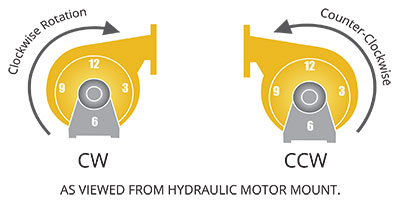
Which direction should my pump be spinning?
Water pumps rotate either clockwise or counterclockwise as viewed from the drive shaft end of the pump. To determine rotation direction position the pump with the shaft end facing yourself. If the outlet of the pump is facing 90 degrees to the right, straight down on the right side of the pump centerline, or straight up on the left side of the pump centerline, then it is a clockwise rotation pump.
If the outlet of the pump is facing 90 degrees to the left, straight down on the left of the pump centerline, or straight up on the right side of the pump centerline, it is a counterclockwise pump.
How often should the water pump bearings be greased?
Water pump bearings should be greased with about 2 oz of grease every 250 hours of service. Most water pumps should only be greased by hand and it should be noted that over greasing can damage bearings as well as no grease.
The water pump shaft is spinning, but there is low/no water pressure. What is wrong?
- Ensure the shaft is spinning in the correct direction. The pump will flow a little bit of water when run backwards. Refer to how to determine whether your pump is clockwise or counterclockwise. All Mega hydraulically driven pumps are clockwise. Only some shaft driven water pumps are counterclockwise.
- Check to see if the impeller is still connected to the shaft.
pump is noisy. What is wrong?
While most water pumps are fairly quiet during operation, hydraulic drive motors can be quite noisy. Ensure that the noise you hear is in fact coming from the water pump. If the pump is making a growling, grinding, squealing, or popping noise, it should be immediately disassembled and inspected for damage
Analogy between a hydraulic circuit (left) and an electronic circuit

HYDRAULIC ANALOGY
The electronic–hydraulic analogy (derisively referred to as the drain-pipe theory by Oliver Lodge) is the most widely used analogy for "electron fluid" in a metal conductor. Since electric current is invisible and the processes at play in electronics are often difficult to demonstrate, the various electronic components are represented by hydraulic equivalents. Electricity (as well as heat) was originally understood to be a kind of fluid, and the names of certain electric quantities (such as current) are derived from hydraulic equivalents. As with all analogies, it demands an intuitive and competent understanding of the baseline paradigms(electronics and hydraulics).
Paradigms
There is no unique paradigm for establishing this analogy. Two paradigms can be used to introduce the concept to students using pressure induced by gravity or by pumps.
In the version with pressure induced by gravity, large tanks of water are held up high, or are filled to differing water levels, and the potential energy of the water head is the pressure source. This is reminiscent of electrical diagrams with an up arrow pointing to +V, grounded pins that otherwise are not shown connecting to anything, and so on. This has the advantage of associating electric potential with gravitational potential.
A second paradigm is a completely enclosed version with pumps providing pressure only and no gravity. This is reminiscent of a circuit diagram with a voltage source shown and the wires actually completing a circuit. This paradigm is further discussed below.
Other paradigms highlight the similarities between equations governing the flow of fluid and the flow of charge. Flow and pressure variables can be calculated in both steady and transient fluid flow situations with the use of the hydraulic ohm analogy. Hydraulic ohms are the units of hydraulic impedance, which is defined as the ratio of pressure to volume flow rate. The pressure and volume flow variables are treated as phasors in this definition, so possess a phase as well as magnitude.
A slightly different paradigm is used in acoustics, where acoustic impedance is defined as a relationship between pressure and air speed. In this paradigm, a large cavity with a hole is analogous to a capacitor that stores compressional energy when the time-dependent pressure deviates from atmospheric pressure. A hole (or long tube) is analogous to an inductor that stores kinetic energy associated with the flow of air.[5]
A circuit was used to model feedback stabilization of a hydrodynamic plasma instability in a magnetic mirror [6] In this application, the effort was to keep the plasma column centered by applying voltages to the plates, and except for the presence of turbulence and non-linear effects, the plasma was an actual electric circuit element (not really an analog).
Hydraulic analogy with horizontal water flow
Voltage, current, and charge

In general, electric potential is equivalent to hydraulic head. This model assumes that the water is flowing horizontally, so that the force of gravity can be ignored. In this case electric potential is equivalent to pressure. The voltage (or voltage drop or potential difference) is a difference in pressure between two points. Electric potential and voltage are usually measured in volts.
Electric current is equivalent to a hydraulic volume flow rate; that is, the volumetric quantity of flowing water over time. Usually measured in amperes.
Electric charge is equivalent to a quantity of water.
Basic circuit elements
.svg)
.svg)

A relatively wide pipe completely filled with water is equivalent to conducting wire. When comparing to a piece of wire, the pipe should be thought of as having semi-permanent caps on the ends. Connecting one end of a wire to a circuit is equivalent to un-capping one end of the pipe and attaching it to another pipe. With few exceptions (such as a high-voltage power source), a wire with only one end attached to a circuit will do nothing; the pipe remains capped on the free end, and thus adds nothing to the circuit.
A resistor is equivalent to a constriction in the bore of the pipe which requires more pressure to pass the same amount of water. All pipes have some resistance to flow, just as all wires have some resistance to current.
A node (or junction) in Kirchhoff's junction rule is equivalent to a pipe tee. The net flow of water into a piping tee (filled with water) must equal the net flow out.


A capacitor is equivalent to a tank with one connection at each end and a rubber sheet dividing the tank in two lengthwise[7] (a hydraulic accumulator). When water is forced into one pipe, equal water is simultaneously forced out of the other pipe, yet no water can penetrate the rubber diaphragm. Energy is stored by the stretching of the rubber. As more current flows "through" the capacitor, the back-pressure (voltage) becomes greater, thus current "leads" voltage in a capacitor. As the back-pressure from the stretched rubber approaches the applied pressure, the current becomes less and less. Thus capacitors "filter out" constant pressure differences and slowly varying, low-frequency pressure differences, while allowing rapid changes in pressure to pass through.
An inductor is equivalent to a heavy paddle wheel placed in the current. The mass of the wheel and the size of the blades restrict the water's ability to rapidly change its rate of flow (current) through the wheel due to the effects of inertia, but, given time, a constant flowing stream will pass mostly unimpeded through the wheel, as it turns at the same speed as the water flow. The mass and surface area of the wheel and its blades are analogous to inductance, and friction between its axle and the axle bearings corresponds to the resistance that accompanies any non-superconducting inductor.
An alternative inductor model is simply a long pipe, perhaps coiled into a spiral for convenience. This fluid-inertia device is used in real life as an essential component of a hydraulic ram. The inertia of the water flowing through the pipe produces the inductance effect; inductors "filter out" rapid changes in flow, while allowing slow variations in current to be passed through. The drag imposed by the walls of the pipe is somewhat analogous to parasitic resistance.
In either model, the pressure difference (voltage) across the device must be present before the current will start moving, thus in inductors voltage "leads" current. As the current increases, approaching the limits imposed by its own internal friction and of the current that the rest of the circuit can provide, the pressure drop across the device becomes lower and lower.
An ideal voltage source (ideal battery) or ideal current source is a dynamic pump with feedback control. A pressure meter on both sides shows that regardless of the current being produced, this kind of pump produces constant pressure difference. If one terminal is kept fixed at ground, another analogy is a large body of water at a high elevation, sufficiently large that the drawn water does not affect the water level. To create the analog of an ideal current source, use a positive displacement pump: A current meter (little paddle wheel) shows that when this kind of pump is driven at a constant speed, it maintains a constant speed of the little paddle wheel.
Other circuit elements
.svg)
.svg)

A diode is equivalent to a one-way check valve with a slightly leaky valve seat. As with a diode, a small pressure difference is needed before the valve opens. And like a diode, too much reverse bias can damage or destroy the valve assembly.
A transistor is a valve in which a diaphragm, controlled by a low-current signal (either constant current for a BJT or constant pressure for a FET), moves a plunger which affects the current through another section of pipe.
CMOS is a combination of two MOSFET transistors. As the input pressure changes, the pistons allow the output to connect to either zero or positive pressure.
A memristor is a needle valve operated by a flow meter. As water flows through in the forward direction, the needle valve restricts flow more; as water flows the other direction, the needle valve opens further providing less resistance.
Principal equivalents
EM wave speed (velocity of propagation) is equivalent to the speed of sound in water. When a light switch is flipped, the electric wave travels very quickly through the wires.
Charge flow speed (drift velocity) is equivalent to the particle speed of water. The moving charges themselves move rather slowly.
DC is equivalent to the a constant flow of water in a circuit of pipes.
Low frequency AC is equivalent to water oscillating back and forth in a pipe
Higher-frequency AC and transmission lines is somewhat equivalent to sound being transmitted through the water pipes, though this does not properly mirror the cyclical reversal of alternating electric current. As described, the fluid flow conveys pressure fluctuations, but fluids do not reverse at high rates in hydraulic systems, which the above "low frequency" entry does accurately describe. A better concept (if sound waves are to be the phenomenon) is that of direct current with high-frequency "ripple" superimposed.
Inductive spark used in induction coils is similar to water hammer, caused by the inertia of water
Equation examples
Some examples of analogous electrical and hydraulic equations:
| type | hydraulic | electric | thermal | mechanical |
|---|---|---|---|---|
| quantity | volume [m3] | charge [C] | heat [J] | momentum [Ns] |
| quantity flux | Volumetric flow rate [m3/s] | current [A=C/s] | heat transfer rate [J/s] | force [N] |
| flux density | velocity [m/s] | current density [C/(m2·s) = A/m²] | heat flux [W/m2] | stress [N/m2 = Pa] |
| potential | pressure [Pa=J/m3=N/m2] | potential [V=J/C=W/A] | temperature [K] | velocity [m/s=J/Ns] |
| linear model | Poiseuille's law | Ohm's law | Fourier's law | dashpot |


If the differential equations have the same form, the response will be similar.
BC. WXO BOND GRAPH
A bond graph is a graphical representation of a physical dynamic system. It allows the conversion of the system into a state-space representation. It is similar to a block diagram or signal-flow graph, with the major difference that the arcs in bond graphs represent bi-directional exchange of physical energy, while those in block diagrams and signal-flow graphs represent uni-directional flow of information. Bond graphs are multi-energy domain (e.g. mechanical, electrical, hydraulic, etc) and domain neutral. This means a bond graph can incorporate multiple domains seamlessly.
The bond graph is composed of the "bonds" which link together "single port", "double-port" and "multi-port" elements (see below for details). Each bond represents the instantaneous flow of energy (dE/dt) or power. The flow in each bond is denoted by a pair of variables called power variables, whose product is the instantaneous power of the bond. The power variables are broken into two parts: flow and effort. For example, for the bond of an electrical system, the flow is the current, while the effort is the voltage. By multiplying current and voltage in this example you can get the instantaneous power of the bond.
A bond has two other features described briefly here, and discussed in more detail below. One is the "half-arrow" sign convention. This defines the assumed direction of positive energy flow. As with electrical circuit diagrams and free-body diagrams, the choice of positive direction is arbitrary, with the caveat that the analyst must be consistent throughout with the chosen definition. The other feature is the "causality". This is a vertical bar placed on only one end of the bond. It is not arbitrary. As described below, there are rules for assigning the proper causality to a given port, and rules for the precedence among ports. Causality explains the mathematical relationship between effort and flow. The positions of the causalities show which of the power variables are dependent and which are independent.
If the dynamics of the physical system to be modeled operate on widely varying time scales, fast continuous-time behaviors can be modeled as instantaneous phenomena by using a hybrid bond graph.

A simple mass–spring–damper system, and its equivalent bond-graph form
Tetrahedron of state

The tetrahedron of state is a tetrahedron that graphically shows the conversion between effort and flow. The adjacent image shows the tetrahedron in its generalized form. The tetrahedron can be modified depending on the energy domain. The table below shows the variables and constants of the tetrahedron of state in common energy domains.
| Energy Domain[2][Note 1] | ||||||||
|---|---|---|---|---|---|---|---|---|
| Generalized | Name | Generalized flow | Generalized effort | Generalized displacement | Generalized momentum | Resistance | Inertance | Compliance |
| Symbol | ||||||||
| Linear
mechanical
| Name | Velocity | Force | Displacement | Linear momentum | Damping constant | Mass | Inverse of the spring constant |
| Symbol | ||||||||
| Units | ||||||||
| Angular
mechanical
| Name | Angular velocity | Torque | Angular displacement | Angular momentum | Angular damping | Mass moment of inertia | Inverse of the angular spring constant |
| Symbol | ||||||||
| Units | ||||||||
| Electromagnetic | Name | Current | Voltage | Charge | Flux linkage | Resistance | Inductance | Capacitance |
| Symbol | ||||||||
| Units | ||||||||
| Hydraulic/
pneumatic
| Name | Volume flow rate | Pressure | Volume | Fluid momentum | Fluid resistance | Fluid inductance | Storage |
| Symbol | ||||||||
| Units | ||||||||


Using the tetrahedron of state, one can find a mathematical relationship between any variables on the tetrahedron. This is done by following the arrows around the diagram and multiplying any constants along the way. For example, if you wanted to find the relationship between generalized flow and generalized displacement, you would start at the f(t) and then integrate it to get q(t). More examples of equations can be seen below.
Relationship between generalized displacement and generalized flow.

Relationship between generalized flow and generalized effort.

Relationship between generalized flow and generalized momentum.

Relationship between generalized momentum and generalized effort.

Relationship between generalized flow and generalized involving the constant C.

All of the mathematical relationships remain the same when switching energy domains, only the symbols change. This can be seen with the following examples.
Relationship between displacement and velocity.

Relationship between current and voltage, this is also known as Ohm's law.

Relationship between force and displacement, also known as Hooke's law. It should be noted that the negative sign is dropped in this equation because the sign is factored into the way the arrow is pointing in the bond graph.

Components
If an engine is connected to a wheel through a shaft, the power is being transmitted in the rotational mechanical domain, meaning the effort and the flow are torque (τ) and angular velocity (ω) respectively. A word bond graph is a first step towards a bond graph, in which words define the components. As a word bond graph, this system would look like:

A half-arrow is used to provide a sign convention, so if the engine is doing work when τ and ω are positive, then the diagram would be drawn:

This system can also be represented in a more general method. This involves changing from using the words, to symbols representing the same items. These symbols are based on the generalized form, as explained above. As the engine is applying a torque to the wheel, it will be represented as a source of effort for the system. The wheel can be presented by an impedance on the system. Further, the torque and angular velocity symbols are dropped and replaced with the generalized symbols for effort and flow. While not necessary in the example, it is common to number the bonds, to keep track of in equations. The simplified diagram can be seen below.

Given that effort is always above the flow on the bond, it is also possible to drop the effort and flow symbols altogether, without losing any relevant information. However, the bond number should not be dropped. The example can be seen below.

The bond number will be important later when converting from the bond graph to state-space equations.
Single-port elements
Single port elements are elements in a bond graph that can have only one port.
Sources and sinks
Sources are elements that represent the input for a system. They will either input effort or flow into a system. They are denoted by a capital "S" with either a lower case "e" or "f" for effort or flow respectively. Sources will always have the arrow pointing away from the element. An examples of sources include: motors (source of effort, torque), voltage sources (source of effort), and current sources (source of flow).

Sinks are elements that represent the output for a system. They are represented the same way as sources, but have the arrow pointing into the element instead of away from it.

Inertance
Inertance elements are denoted by a capital "I", and always have power flowing into them. Inertance elements are elements that store kinetic energy. Most commonly these are a mass for mechanical systems, and inductors for electrical systems.

Resistance
Resistance elements are denoted by a capital "R", and always have power flowing into them. Resistance elements are elements that dissipate energy. Most commonly these are a dampener, for mechanical systems, and resistors for electrical systems.

Capacitance
Capacitance elements are denoted by a capital "C", and always have power flowing into them. Capacitance elements are elements that store potential energy. Most commonly these are springs for mechanical systems, and capacitors for electrical systems.

Two-port elements
These elements have two ports. They are used to change the power between or within a system. When converting from one to the other, no power is lost during the transfer. The elements have a constant that will be given with it. The constant is called a transformer constant or gyrator constant depending on which element is being used. These constants will commonly be displayed as a ratio below the element.
Transformer
A transformer applies a relationship between flow in flow out, and effort in effort out. Examples include an ideal electrical transformer or a lever.
Denoted

where the r denotes the modulus of the transformer. This means

and

Gyrator
A gyrator applies a relationship between flow in effort out, and effort in flow out. An example of a gyrator is a DC motor, which converts voltage (electrical effort) into Angular velocity (angular mechanical flow).

meaning that

and

Multi-port elements
Junctions, unlike the other elements can have any number of ports either in or out. Junctions split power across their ports. There are two distant junctions, the 0-junction and the 1-junction which differ only in the how effort and flow are carried across. It should be noted that the same junction in series can be combined, but different junctions in series cannot.
0-junctions
0-junctions behave such that all efforts values are equal across the bonds, but the sum of the flow values in equals the sum the flow values out.


An example is shown below.

Resulting equations:


1-junctions
1-junctions behave opposite of 0-junctions. 1-junctions behave such that all flow values are equal across the bonds, but the sum of the effort values in equals the sum the effort values out.


An example is shown below.

Resulting equations:


Causality
Bond graphs have a notion of causality, indicating which side of a bond determines the instantaneous effort and which determines the instantaneous flow. In formulating the dynamic equations that describe the system, causality defines, for each modeling element, which variable is dependent and which is independent. By propagating the causation graphically from one modeling element to the other, analysis of large-scale models becomes easier. Completing causal assignment in a bond graph model will allow the detection of modeling situation where an algebraic loop exists; that is the situation when a variable is defined recursively as a function of itself.
As an example of causality, consider a capacitor in series with a battery. It is not physically possible to charge a capacitor instantly, so anything connected in parallel with a capacitor will necessarily have the same voltage (effort variable) as the capacitor. Similarly, an inductor cannot change flux instantly and so any component in series with an inductor will necessarily have the same flow as the inductor. Because capacitors and inductors are passive devices, they cannot maintain their respective voltage and flow indefinitely—the components to which they are attached will affect their respective voltage and flow, but only indirectly by affecting their current and voltage respectively.
Note: Causality is a symmetric relationship. When one side "causes" effort, the other side "causes" flow.
In bond graph notation, a causal stroke may be added to one end of the power bond to indicate that the opposite end is defining the effort. Consider a constant-torque motor driving a wheel, i.e. a source of effort (SE). That would be drawn as follows:
![\begin{array}[b]{r}\text{motor}\\SE\end{array}\;
\overset{\textstyle\tau}{\underset{\textstyle\omega}{-\!\!\!-\!\!\!-\!\!\!\rightharpoonup\!\!\!|}}\;\text{wheel}](https://wikimedia.org/api/rest_v1/media/math/render/svg/de6dfde02c6c4d3de8d5caa7b60c31a845830392)
Symmetrically, the side with the causal stroke (in this case the wheel) defines the flow for the bond.
Causality results in compatibility constraints. Clearly only one end of a power bond can define the effort and so only one end of a bond can have a causal stroke. In addition, the two passive components with time-dependent behavior, I and C, can only have one sort of causation: an I component determines flow; a C component defines effort. So from a junction, J, the preferred causal orientation is as follows:

The reason that this is the preferred method for these elements can be further analyzed if you consider the equations they would give shown by the tetrahedron of state.

The resulting equations involve the integral of the independent power variable. This is preferred over the result of having the causality the other way, which results in derivative. The equations can be seen below.

It is possible for a bond graph to have a casual bar on one of these elements in the non-preferred manner. In such a case a "casual conflict" is said to have occurred at that bond. The results of a causal conflict are only seen when writing the state-space equations for the graph. It is explained in more details in that section.
A resistor has no time-dependent behavior: apply a voltage and get a flow instantly, or apply a flow and get a voltage instantly, thus a resistor can be at either end of a causal bond:

Sources of flow (SF) define flow, sources of effort (SE) define effort. Transformers are passive, neither dissipating nor storing energy, so causality passes through them:

A gyrator transforms flow to effort and effort to flow, so if flow is caused on one side, effort is caused on the other side and vice versa:
- Junctions

In a 0-junction, efforts are equal; in a 1-junction, flows are equal. Thus, with causal bonds, only one bond can cause the effort in a 0-junction and only one can cause the flow in a 1-junction. Thus, if the causality of one bond of a junction is known, the causality of the others is also known. That one bond is called the 'strong bond'

Determining causality
In order to determine the causality of a bond graph certain steps must be followed. Those steps are:
- Draw Source Causal Bars
- Draw Preferred causality for C and I bonds
- Draw causal bars for 0 and 1 junctions, transformers and gyrators
- Draw R bond causal bars
- If a causal conflict occurs, change C or I bond to differentiation
A walk-through of the steps is shown below.

The first step is to draw causality for the sources, over which there is only one. This results in the graph below.

The next step is to draw the preferred causality for the C bonds.

Next apply the causality for the 0 and 1 junctions, transformers, and gyrators.

However, it should be noted that there is an issue with 0-junction on the left. The 0-junction has two causal bars at the junction, but the 0-junction wants one and only one at the junction. This was caused by having be in the preferred causality. The only way to fix this is to flip that causal bar. This results in a causal conflict, the corrected version of the graph is below, with the representing the causal conflict.


Converting from other systems
One of the main advantages of using bond graphs is that once you have a bond graph it doesn't matter the original energy domain. Below are some of the steps to apply when converting from the energy domain to a bond graph.
Electromagnetic
The steps for solving an Electromagnetic problem as a bond graph are as follows:
- Place an 0-junction at each node
- Insert Sources, R, I, C, TR, and GY bonds with 1 junctions
- Ground (both sides if a transformer or gyrator is present)
- Assign power flow direction
- Simplify
These steps are shown more clearly in the examples below.
Linear mechanical
The steps for solving an Linear Mechanical problem as a bond graph are as follows:
- Place 1-junctions for each distinct velocity (usually at a mass)
- Insert R and C bonds at their own 0-junctions between the 1 junctions where they act
- Insert Sources and I bonds on the 1 junctions where they act
- Assign power flow direction
- Simplify
These steps are shown more clearly in the examples below.
Simplifying
The simplifying step is the same regardless if the system was electromagnetic or linear mechanical. The steps are:
- Remove Bond of zero power (due to ground or zero velocity)
- Remove 0 and 1 junctions with less than three bonds
- Simplify parallel power
- Combine 0 junctions in series
- Combine 1 junctions in series
These steps are shown more clearly in the examples below.
Parallel power
Parallel power is when power runs in parallel in a bond graph. An example of parallel power is shown below.

Parallel power can be simplified, by recalling the relationship between effort and flow for 0 and 1-junctions. To solve parallel power you will first want to write down all of the equations for the junctions. For the example provided, the equations can be seen below. (Please make note of the number bond the effort/flow variable represents).

By manipulating these equations you can arrange them such that you can find an equivalent set of 0 and 1-junctions to describe the parallel power.
For example because and you can replace the variables in the equation resulting in and since


, we now know that . This relationship of two effort variables equaling can explained by an 0-junction. Manipulating other equations you can find that which describes the relationship of a 1-junction. Once you have determined the relationships that you need you can redraw the parallel power section with the new junctions. The result for the example show is seen below.


Examples
Simple electrical system
A simple electrical circuit consisting of a voltage source, resistor, and capacitor in series.

The first step is to draw 0-junctions at all of the node. The result is shown below.

The next step is to add all of the elements acting at their own 1-junction. The result is below.

The next step is to pick a ground. The ground is simply an 0-junction that is going to be assumed to have no voltage. For this case, the ground will be chosen to be the lower left 0-junction, that is underlined above. The next step is to draw all of the arrows for the bond graph. The arrows on junctions should point towards ground (following a similar path to current). For resistance, inertance, and compliance elements, the arrows always point towards the elements. The result of drawing the arrows can be seen below, with the 0-junction marked with a star as the ground.

Now that we have the Bond graph, we can start the process of simplifying it. The first step is to remove all the ground nodes. Both of the bottom 0-junctions can be removed, because they are both grounded. The result is shown below.

Next, the junctions with less than three bonds can be removed. This is because flow and effort pass through these junctions without be modified, so they can be removed to allow us to draw less. The result can be seen below.

The final step is to apply causality to the bond graph. Applying causality was explained above. The final bond graph is shown below.

Advanced electrical system
A more advanced electrical system with a current source, resistors, capacitors, and a transformer

Following the steps with this circuit will result in the bond graph below, before it is simplified. The nodes marked with the star denote the ground.

Simplifying the bond graph will result in the image below.

Lastly, applying causality will result in the bond graph below. It should be noted that the bond with star denotes a causal conflict.

Simple linear mechanical
A simple linear mechanical system, consisting of a mass on a spring that is attached to a wall. The mass has some force being applied to it. An image of the system is shown below.

For a mechanical system, the first step is to place a 1-junction at each distant velocity, in this case there are two distant velocities, the mass and the wall. It is usually helpful to label the 1-junctions for reference. The result is below.

The next step is to draw the R and C bonds at their own 0-junctions between the 1-junctions where they act. For this example there is only one of these bonds, the C bond for the spring. It acts between the 1-junction representing the mass and the 1-junction representing the wall. The result is below.

Next you want to add the sources and I bonds on the 1-junction where they act. There is one source, the source of effort (force) and one I bond, the mass of the mass both of which act on the 1-junction of the mass. The result is shown below.

Next you want to assign power flow. Like the electrical examples, power should flow towards ground, in this case the 1-junction of the wall. Exceptions to this are R,C, or I bond, which always point towards the element. The resulting bond graph is below.

Now that the bond graph has been generated, it can be simplified. Because the wall is grounded (has zero velocity), you can remove that junction. As such the 0-junction the C bond is on, can also be removed because it will then have less than three bonds. The simplified bond graph can be seen below.

The last step is to apply causality, the final bond graph can be seen below.

Advanced linear mechanical
A more advanced linear mechanical system can be seen below.

Just like the above example, the first step is to make 1-junctions at each of the distant velocities. In this example there are three distant velocity, Mass 1, Mass 2, and the wall. Then you connect all of the bonds and assign power flow. The bond can be seen below.

Next you start the process of simplifying the bond graph, by removing the 1-junction of the wall, and removing junctions with less than three bonds. The bond graph can be seen below.

It should be noted that there is parallel power in the bond graph. Solving parallel power was explained above. The result of solving it can be seen below.

Lastly, apply causality, the final bond graph can be seen below.

State equations
Once a bond graph is complete, it can be utilized to generate the state-space representation equations of the system. State-space representation is especially powerful as it allows complex multi-order differential system to be solved as a system of first-order equations instead. The general form of the state equation can be seen below.

Where, is a column matrix of the state variables, or the unknowns of the system. is the time derivative of the state variables. is a column matrix of the inputs of the system. And and are matrices of constants based on the system. The state variables of a system are and values for each C and I bond without a causal conflict. Each I bond gets a while each C bond gets a .


For example, if you have the bond graph shown below.

Would have the following , , and matrices.
![{\displaystyle {\dot {\textbf {x}}}(t)=\left[{\begin{matrix}{\dot {p}}_{3}(t)\\{\dot {q}}_{6}(t)\end{matrix}}\right]\qquad {\text{and}}\qquad {\textbf {x}}(t)=\left[{\begin{matrix}p_{3}(t)\\q_{6}(t)\end{matrix}}\right]\qquad {\text{and}}\qquad {\textbf {u}}(t)=\left[{\begin{matrix}e_{1}(t)\end{matrix}}\right]}](https://wikimedia.org/api/rest_v1/media/math/render/svg/2d34aa1cd7d3a785219e84ff8198580a54fea761)
The matrices of and are solved by determining the relationship of the state variables and their respective elements, as was described in the tetrahedron of state. The first step to solve the state equations, is to list all of the governing equations for the bond graph. The table below, shows the relationship between bonds and their governing equations.
| Bond Name | Bond with
Causality
| Governing Equation(s) | |
|---|---|---|---|
| "♦" denotes preferred causality | |||
| One Port
Elements
| Source/ Sink, S | ||
| Resistance, R:
Dissipated Energy
| |||
| Inertance, I:
Kinetic Energy
| ♦ | ||
| Compliance, C:
Potential Energy
| |||
| ♦ | |||
| Two Port
Elements
| Transformer, TR | ||
| Gyrator, GY | |||
| Multi-port
Elements
| 0 junction | One and only one
causal bar at the junction
| |
| 1 junction | one and only one causal
bar away from the junction
| ||


For the example provided,
The governing equations are the following.

These equations can be manipulated to yield the state equations. For this example, you are trying to find equations that relate and in terms of , , and .


To start you should recall from the tetrahedron of state that starting with equation 2, you can rearrange it so that . can be substituted for equation 4, while in equation 4, can be replaced by due to equation 3, which can then be replaced by equation 5. can likewise be replaced using equation 7, in which can be replaced with which can then be replaced with equation 10. Following these substituted yields the first state equation which is shown below.


The second state equation can likewise be solved, by recalling that . The second state equation is shown below.


Both equations can further be rearranged into matrix form. The result of which is below.

At this point the equations can be treated as any other state-space representation problem.
PMW Low-Side Driver for Solenoids
CD. WXO Electronic Valve Aircraft System


Capacitive fuel quantity system
The majority of turbine-powered aircraft fuel quantity indicating systems (FQIS) use the capacitive fuel quantity system. On a typical twin-engine passenger aircraft the fuel tanks are contained within the aircraft structure as shown in FIG. 5. Fuel tank sensors are located throughout each tank and are monitored by an electronic control system. Accurate readings can be obtained by capacitive fuel quantity systems in large and irregular-shaped tanks.
2.4.1 Principle of operation
Fuel tank units are formed by concentric aluminum tubes; the inner and outer tubes are the capacitor plates, see FIG. 6. The primary advantages of this technology are no moving parts and fuel quantity is measured in mass rather than volume. (The mass of fuel determines the amount of energy available.) The dielectric is either fuel or air depending on the quantity of fuel in tank. Air has a dielectric of 1.0006 (practically unity); fuel has a dielectric of approximately two; this provides a good relationship for the measurement of a variable quantity.
From basic fundamentals, we know that capacitance is proportional to:
-- plate area
-- air gap
-- dielectric strength
In the capacitive tank unit, the first two parameters are fixed; the capacitance varies in accordance with the dielectric, i.e. the amount of fuel in the tank as illustrated in FIG. 7. With a high quantity of fuel in the tank, the capacitance is high; capacitance varies in direct proportion to the amount of fuel in the tank.
The tank's capacitance unit is connected into an impedance bridge circuit, see FIG. 8. Variation in capacitance ( C ) of the fuel tank unit causes a change in reactance ( XC ); this is given by the formula: XFC C _ 1 2 p
...where XC is the reactance, ? is a constant, F is the frequency (400 Hz from the aircraft power supply) and C is the capacitance. The impedance ( Z ) of a capacitive network can be calculated from the formula: ZRX __ v( 22 c )
The current in a capacitive network can now be calculated from the formula: I V Z
When the fuel is consumed during a flight, and the fuel level decreases, the capacitance decreases and the reactance increases; less current flows in the tank unit (compared with the reference capacitor). This unbalance causes a potential difference at points X-Y, proportional to fuel quantity; this signal is amplified and used to drive an indicator. Capacitance trimmers are used for calibration of the fuel indicators (or gauges).
Key point: Air and fuel have dielectrics of approximately unity and two respectively.


JET AIRCRAFT ENGINE LUBRICATION

Working of Fuel Injection Pump compare to
Fuel transfer of AIRCRAFT
This system is used to selectively transfer fuel between tanks; electrically driven fuel pumps and motorized valves are controlled either manually by the crew or by an automatic control system. A simple example of this is illustrated in FIG. 13, where fuel can be cross-fed between the left and right tanks.
On larger aircraft, the complexity of this fuel transfer system increases. The system comprises a number of motorized valves. Engine valves are activated by the start lever or fire handles. The left, center and right refuel/defuel valves are operated from an under-wing panel. Bypass valves (BPV) are operated if an electrical pump's fuel filter is blocked. (The BPV senses differential pressure across the filter.) Controls and indications are located on an overhead panel or flight engineer's station. An electrically operated cross-feed valve normally closed unless fuel is being transferred.
It is essential that fuel temperature is monitored, either manually or automatically. The maximum fuel temperature is typically _ 49°C; the minimum fuel temperature is -45ºC or freezing point _ 3ºC, whichever is higher; the typical freezing point of Jet A1 fuel is _ 47ºC. Fuel temperature is measured by an RTD. If the fuel temperature is approaching the lower limits, some fuel could be transferred between tanks; alternatively the aircraft would have to descend into warmer air or accelerate to increase the kinetic heating.
Refueling and defueling
A refueling control panel and pressure connections are normally located in one or both of the wing areas allowing the fuel to be supplied directly into the main fuel system. A bonding lead is always connected between the fuel bowser and aircraft to minimize the risk of static discharge. The fuel tank supply line is connected to the aircraft and pressure applied. Selective control of the system's motorized valves allow specific tanks to be filled as required.
Defueling is often required before maintenance, or if the aircraft is to be weighed. The fuel is transferred from the aircraft into a suitable container, typically a fuel bowser. This is achieved via a defueling valve and applying suction through valves.
Fuel jettison
When an aircraft takes off fully loaded with passengers and fuel, and then needs to make an emergency landing, it will almost certainly be over its maximum landing weight. Fuel has to be disposed of to reduce the aircraft weight to prepare for the emergency landing. A large aircraft such as the Boeing 747 can be carrying over 100 tonnes of fuel; this is almost 50% of the aircraft's gross weight. One way of burning off fuel and reducing aircraft weight is to fly in a high drag configuration, e.g. 250 knots with the gear down (speed-brakes will further increase the drag). Aircraft can be certified for landings up to the maximum takeoff weight (MTOW) in an emergency; however, overweight landings would only be made if burning off fuel exposed the aircraft to additional hazards.
Some aircraft are installed with a fuel jettison, or fuel dumping system . This provides a means of pumping fuel overboard to rapidly decrease the aircraft's weight. Fuel can normally be jettisoned with landing gear and/or flaps extended. Two jettison pumps are installed in each main tank, fuel is pumped via a jettison manifold to nozzle valves located at each wing tip trailing edge.
Key maintenance point: Bonding of fuel system components is essential to ensure intrinsic safety.
Fuel tank venting
The venting system takes ram air from intakes on the underside of the wing for two specific purposes.
When the aircraft is flying, ram air is used to pressurize the fuel to prevent vaporization at lower atmospheric pressures. The ram air also pressurizes the fuel tanks to ensure positive pressure on the inlet ports of each pump. The expansion space above the fuel, called ullage, changes with aircraft attitude. Float operated vent valves are located at Key points in the tank to allow fuel to escape into the vent system.
Venting tanks (sometimes called surge tanks ) in the wing tips collect this overspill from the main tanks; the fuel is then pumped back into one of the main tanks. Float-operated vent valves prevent inadvertent transfer of fuel between the tanks.
========

FIG. Fuel jettison system schematic; No. 2 main tank
To right wing manifold Surge tank No.2 reserve tank No.1 reserve tank No.1 main tank Inlet Fuel Center wing tank Center wing tank jettison valve No. 2 main jettison pumps No. 2 main tank Main tank transfer valve No.1 reserve tank transfer valve No.2 reserve tank transfer valve Fuel Jettison nozzle valve Fuel Jettison nozzle Center wing tank jettison valve Center wing override/ jettison pumps
Fuel tank inerting
Aircraft have been destroyed due to explosions in empty center wing fuel tanks. The most likely cause is the center tank fuel pumps being left running in high ambient temperatures with low fuel quantity. The first center wing tank (CWT) explosion on a large passenger aircraft occurred on a B707 in 1959; there have been other events in more recent times. In May 1990, shortly after pushback, the center wing tank (CWT) exploded on a Philippine Airlines Boeing 737, killing eight people. The CWT had not been filled since March 9, 1990. Air-conditioning (A/C) packs had been running on the ground before pushback for approximately 30 to 45 minutes, ambient air was 35°C/95°F. On March 3, 2001, the center wing tank explosion on Thai Airways International B737 was followed 18 minutes later by an explosion in the right wing tank. Residual fuel was in the CWT. Air-conditioning packs had been running continuously since the air craft's previous flight, including some 40 minutes on the ground. Ambient air temperature was in excess of 30°C. On July 17, 1996, the CWT exploded on a TWA B747-100 shortly after takeoff from JFK International Airport with fatal consequences. The CWT contained a low amount of residual fuel. The A/C packs had been running on the ground for 2.5 hours before takeoff, ambient temperature was 28°C/82°F. These three fatal CWT fuel-tank explosions all had certain elements in common:
-- all three aircraft had only a small amount of fuel in the wing tank
-- the air-conditioning packs, located in non-vented bays directly under the CWT, had been running before the explosions
-- the outside air temperatures were quite warm.
A small amount of fuel in the center wing tank means that there is a large volume for fuel vapor to occupy.
Air-conditioning packs generate heat, which contributes to fuel vaporization in the non-insulated tanks.
The vaporization is increased with high outside air temperatures.
Empty fuel tanks retain some unusable fuel which, in high ambient temperature conditions, will evaporate and create an explosive mixture when combined with oxygen in the ullage. Regulatory mandates have introduced improvements to the design and maintenance of fuel tanks to reduce the chances of such explosions. These improvements include the enhanced design of the FQIS and fuel pumps, inspection regimes for wiring in the tanks and insulating fuel tanks that are in close proximity to sources of high temperature. The longer-term solution that will contribute more towards fuel tank safety is inerting ; possible solutions include:
-- ground-based inerting
-- on-board ground inerting
-- on-board inert gas generation system (OBIGGS)
-- liquid nitrogen from a ground source
For ground-based inerting, the fuel tanks would receive an amount of nitrogen-enriched air before pushback.
Inerting would last for the taxi, takeoff and climb phases of flight, when the fuel vapors would be warmest. On board ground inerting achieves the same objective; however, the inerting equipment is an aircraft system.
Although OBIGGS offers tremendous benefits, it is expensive. Nitrogen generating systems (NGS) have been developed which decrease the flammability risks of the tanks. The NGS is an onboard inert gas system; external (atmospheric) air is directed into an air separation module (ASM), this separates out the oxygen and nitrogen via a molecular sieve. After separation, the nitrogen-enriched air (NEA) is supplied into the center wing tank and the oxygen-enriched air (OEA) is vented overboard. NEA decreases the oxygen content in the ullage to prevent combustion. Trials have determined that an oxygen level of 12% is sufficient to prevent ignition; this is achievable with one ASM on a medium sized aircraft and up to six ASMs on larger wide-bodied aircraft.
In the fourth potential method, the aircraft would receive a supply of liquid nitrogen from a ground source. The liquid nitrogen would be stored on the aircraft in a vacuum-sealed insulated container, and would be fed to the fuel tanks under low pressure.
Oxygen sensors in the fuel tanks provide feedback to the system's computer control function; the supply of liquid nitrogen is regulated to keep the fuel tanks inerted for critical phases of flight. The liquid nitro gen could also be used to supplement fire suppression in other areas of the aircraft. A computer would monitor temperature in the fuel tanks to determine if the ullage is within a flammable temperature range. This system would know the tank temperature at all times, together with the oxygen content of the tanks.
There remains an on-going industry debate regarding the effectiveness and cost of inerting. There needs to be a practical means of inerting fuel tanks for in service and new-production civil transports.