Equation of time in complete function
Thankyume the equation of time describes the discrepancy between two kinds of solar time. The word equation is used in the medieval sense of reconcile a difference. The two times that differ are the apparent solar time, which directly tracks the motion of the sun, and mean solar time, which tracks a theoretical "mean" sun with noons 24 hours apart. Apparent (or true) solar time can be obtained by measurement of the current position (hour angle) of the Sun, as indicated (with limited accuracy) by a sundial. Mean solar time, for the same place, would be the time indicated by a steady clock set so that over the year its differences from apparent solar time would resolve to zero.
The equation of time is the east or west component of the analemma, a curve representing the angular offset of the Sun from its mean position on the celestial sphere as viewed from Earth. The equation of time values for each day of the year, compiled by astronomical observatories, were widely listed in almanacs and ephemerides.
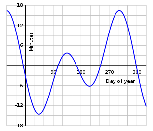
The equation of time — above the axis a sundial will appear fast relative to a clock showing local mean time, and below the axis a sundial will appear slow.
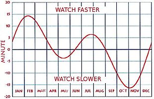
and then This graph uses the opposite sign to the one above it. There is no universally followed convention for the sign of the equation of time.
The concept
During a year the equation of time varies as shown on the graph; its change from one year to the next is slight. Apparent time, and the sundial, can be ahead (fast) by as much as 16 min 33 s (around 3 November), or behind (slow) by as much as 14 min 6 s (around 12 February). The equation of time has zeros near 15 April, 13 June, 1 September and 25 December. Ignoring very slow changes in the Earth's orbit and rotation, these events are repeated at the same times every tropical year. However, due to the non-integer number of days in a year, these dates can vary by a day or so from year to year.
The graph of the equation of time is closely approximated by the sum of two sine curves, one with a period of a year and one with a period of half a year. The curves reflect two astronomical effects, each causing a different non-uniformity in the apparent daily motion of the Sun relative to the stars:
- the obliquity of the ecliptic (the plane of the Earth's annual orbital motion around the Sun), which is inclined by about 23.44 degrees relative to the plane of the Earth'sequator; and
- the eccentricity of the Earth's orbit around the Sun, which is about 0.0167.
The equation of time is constant only for a planet with zero axial tilt and zero orbital eccentricity. On Mars the difference between sundial time and clock time can be as much as 50 minutes, due to the considerably greater eccentricity of its orbit. The planet Uranus, which has an extremely large axial tilt, has an equation of time that makes its days start and finish several hours earlier or later depending on the time of its solar year orbital period.
Apparent time versus mean time
Until the invention of the pendulum and the development of reliable clocks during the 17th century, the equation of time as defined by Ptolemy remained a curiosity, of importance only to astronomers. However, when mechanical clocks started to take over timekeeping from sundials, which had served humanity for centuries, the difference between clock time and solar time became an issue for everyday life. Apparent solar time (or true or real solar time) is the time indicated by the Sun on a sundial (or measured by its transit over a preferred local meridian), while mean solar time is the average as indicated by well-regulated clocks. The first tables to give the equation of time in an essentially correct way were published in 1665 by Christiaan Huygens. Huygens, following the tradition of Ptolemy and medieval astronomers in general, set his values for the equation of time so as to make all values positive throughout the year.
Another set of tables was published in 1672–73 by John Flamsteed who later became the first Astronomer Royal of the new Greenwich Observatory. These appear to have been the first essentially correct tables that gave today's meaning of Mean Time (rather than mean time based on the latest sunrise of the year as proposed by Huygens). Flamsteed adopted the convention of tabulating and naming the correction in the sense that it was to be applied to the apparent time to give mean time.
The equation of time, correctly based on the two major components of the Sun's irregularity of apparent motion,was not generally adopted until after Flamsteed's tables of 1672–73, published with the posthumous edition of the works of Jeremiah Horrocks.
Robert Hooke (1635–1703), who mathematically analyzed the universal joint, was the first to note that the geometry and mathematical description of the (non-secular) equation of time and the universal joint were identical, and proposed the use of a universal joint in the construction of a "mechanical sundial".
 Graph showing the equation of time (red solid line) along with its two main components plotted separately, the part due to the obliquity of the ecliptic (mauve dashed line) and the part due to the Sun's varying apparent speed along the ecliptic due to the eccentricity of the Earth's orbit (dark blue dash & dot line) Sun and planets at solar midday (Ecliptic in red, Sun and Mercury in yellow, Venus in white, Mars in red, Jupiter in yellow with red spot, Saturn in white with rings).
Secular effects[edit]
The two above mentioned factors have different wavelengths, amplitudes and phases, so their combined contribution is an irregular wave. Atepoch 2000 these are the values (in minutes and seconds with UT dates):
| Point | Value | Date |
|---|---|---|
| minimum | −14 min 15 s | 11 February |
| zero | 0 min 0 s | 15 April |
| maximum | +3 min 41 s | 14 May |
| zero | 0 min 0 s | 13 June |
| minimum | −6 min 30 s | 26 July |
| zero | 0 min 0 s | 1 September |
| maximum | +16 min 25 s | 3 November |
| zero | 0 min 0 s | 25 December |
- E.T. = apparent − mean. Positive means: Sun runs fast and culminates earlier, or the sundial is ahead of mean time. A slight yearly variation occurs due to presence of leap years, resetting itself every 4 years.
The exact shape of the equation of time curve and the associated analemma slowly change over the centuries, due to secular variations in both eccentricity and obliquity. At this moment both are slowly decreasing, but they increase and decrease over a timescale of hundreds of thousands of years. If and when the Earth's orbital eccentricity (now about 0.0167 and slowly decreasing) reaches 0.047, the eccentricity effect may in some circumstances overshadow the obliquity effect, leaving the equation of time curve with only one maximum and minimum per year, as is the case on Mars.
On shorter timescales (thousands of years) the shifts in the dates of equinox and perihelion will be more important. The former is caused by precession, and shifts the equinox backwards compared to the stars. But it can be ignored in the current discussion as our Gregorian calendar is constructed in such a way as to keep the vernal equinox date at 21 March (at least at sufficient accuracy for our aim here). The shift of the perihelion is forwards, about 1.7 days every century. In 1246 the perihelion occurred on 22 December, the day of the solstice, so the two contributing waves had common zero points and the equation of time curve was symmetrical: in Astronomical Algorithms Meeus gives February and November extrema of 15 m 39 s and May and July ones of 4 m 58 s. Before that time the February minimum was larger than the November maximum, and the May maximum larger than the July minimum. In fact, in years before −1900 (1901 BCE) the May maximum was larger than the November maximum. In the year −2000 (2001 BCE) the May maximum was +12 minutes and a couple seconds while the November maximum was just less than 10 minutes.

Calculating the equation of time
The equation of time is obtained from a published table, or a graph. For dates in the past such tables are produced from measurements done at the time, or by calculation; for future dates, of course, tables can only be calculated. In devices such as computer-controlled heliostats the computer is often programmed to calculate the equation of time. The calculation can be numerical or analytical. The former are based on numerical integration of the differential equations of motion, including all significant gravitational and relativistic effects. The results are accurate to better than 1 second and are the basis for modern almanac data. The latter are based on a solution that includes only the gravitational interaction between the Sun and Earth, simpler than but not as accurate as the former. Its accuracy can be improved by including small corrections.
The following discussion describes a reasonably accurate (agreeing with Almanac data to within 3 seconds over a wide range of years) algorithm for the equation of time that is well known to astronomers. It also shows how to obtain a simple approximate formula (accurate to within 1 minute over a large time interval), that can be easily evaluated with a calculator and provides the simple explanation of the phenomenon that was used previously in this article.
Mathematical description
The precise definition of the equation of time is
- EOT = GHA − GMHA
The quantities occurring in this equation are
- EOT, the time difference between apparent solar time and mean solar time;
- GHA, the Greenwich Hour Angle of the apparent (actual) Sun;
- GMHA = Universal Time − Offset, the Greenwich Mean Hour Angle of the mean (fictitious) Sun.
Here time and angle are quantities that are related by factors such as: 2π radians = 360° = 1 day = 24 hours. The difference, EOT, is measurable since GHA is an angle that can be measured and Universal Time, UT, is a scale for the measurement of time. The offset by π = 180° = 12 hours from UT is needed because UT is zero at mean midnight while GMHA = 0 at mean noon. Both GHA and GMHA, like all physical angles, have a mathematical, but not a physical discontinuity at their respective (apparent and mean) noon. Despite the mathematical discontinuities of its components, EOT is defined as a continuous function by adding (or subtracting) 24 hours in the small time interval between the discontinuities in GHA and GMHA.
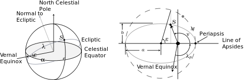
The celestial sphere and the Sun's elliptical orbit as seen by a geocentric observer looking normal to the ecliptic showing the 6 angles (M, λp, α, ν, λ, E) needed for the calculation of the equation of time. For the sake of clarity the drawings are not to scale.
Speed Controllers in time
Introduction
The purpose of a motor speed controller is to take a signal representing the demanded speed, and to drive a motor at that speed. The controller may or may not actually measure the speed of the motor. If it does, it is called a Feedback Speed Controller or Closed Loop Speed Controller, if not it is called an Open Loop Speed Controller. Feedback speed control is better, but more complicated, and may not be required for a simple robot design.
Motors come in a variety of forms, and the speed controller's motor drive output will be different dependent on these forms. The speed controller presented here is designed to drive a simple cheap starter motor from a car, which can be purchased from any scrap yard. These motors are generally series wound, which means to reverse them, they must be altered slightly,
Below is a simple block diagram of the speed controller. We'll go through the important parts block by block in detail.

Theory of DC motor speed control
The speed of a DC motor is directly proportional to the supply voltage, so if we reduce the supply voltage from 12 Volts to 6 Volts, the motor will run at half the speed. How can this be achieved when the battery is fixed at 12 Volts?
The speed controller works by varying the average voltage sent to the motor. It could do this by simply adjusting the voltage sent to the motor, but this is quite inefficient to do. A better way is to switch the motor's supply on and off very quickly. If the switching is fast enough, the motor doesn't notice it, it only notices the average effect.
When you watch a film in the cinema, or the television, what you are actually seeing is a series of fixed pictures, which change rapidly enough that your eyes just see the average effect - movement. Your brain fills in the gaps to give an average effect.
Now imagine a light bulb with a switch. When you close the switch, the bulb goes on and is at full brightness, say 100 Watts. When you open the switch it goes off (0 Watts). Now if you close the switch for a fraction of a second, then open it for the same amount of time, the filament won't have time to cool down and heat up, and you will just get an average glow of 50 Watts. This is how lamp dimmers work, and the same principle is used by speed controllers to drive a motor. When the switch is closed, the motor sees 12 Volts, and when it is open it sees 0 Volts. If the switch is open for the same amount of time as it is closed, the motor will see an average of 6 Volts, and will run more slowly accordingly.
As the amount of time that the voltage is on increases compared with the amount of time that it is off, the average speed of the motor increases.
This on-off switching is performed by power MOSFETs. A MOSFET (Metal-Oxide-Semiconductor Field Effect Transistor) is a device that can turn very large currents on and off under the control of a low signal level voltage.
The time that it takes a motor to speed up and slow down under switching conditions is dependant on the inertia of the rotor (basically how heavy it is), and how much friction and load torque there is. The graph below shows the speed of a motor that is being turned on and off fairly slowly:

You can see that the average speed is around 150, although it varies quite a bit. If the supply voltage is switched fast enough, it won’t have time to change speed much, and the speed will be quite steady. This is the principle of switch mode speed control. Thus the speed is set by PWM – Pulse Width Modulation.
Inductors
Before we go on to discuss the circuits, we must first learn something about the action of inductive loads, and inductors. Inductors do not allow the current flowing through them to change instantly (in the same way capacitors do not allow the voltage across them to change instantly). The voltage dropped across an inductor carrying a current i is given by the equation

where di/dt is the rate of change of the current. If the current is suddenly changed by opening a switch, or turning a transistor off, the inductor will generate a very high voltage across it. For example, turning off 100 Amps in 1 microsecond through a 100 microHenry inductor generates 10kV!
PWM frequency
The frequency of the resulting PWM signal is dependant on the frequency of the ramp waveform. What frequency do we want? This is not a simple question. Some pros and cons are:
- Frequencies between 20Hz and 18kHz may produce audible screaming from the speed controller and motors - this may be an added attraction for your robot!
- RF interference emitted by the circuit will be worse the higher the switching frequency is.
- Each switching on and off of the speed controller MOSFETs results in a little power loss. Therefore the greater the time spent switching compared with the static on and off times, the greater will be the resulting 'switching loss' in the MOSFETs.
- The higher the switching frequency, the more stable is the current waveform in the motors. This waveform will be a spiky switching waveform at low frequencies, but at high frequencies the inductance of the motor will smooth this out to an average DC current level proportional to the PWM demand. This spikyness will cause greater power loss in the resistances of the wires, MOSFETs, and motor windings than a steady DC current waveform.
This third point can be seen from the following two graphs. One shows the worst case on-off current waveform, the other the best case steady DC current waveform:

Both waveforms have the same average current. However, when we work out the power dissipation in the stray resistances in our motor and speed controller, for the DC case:

and for the switching case, the average power is

So in the switching waveform, twice as much power is lost in the stray resistances. In practice the current waveform will not be square wave like this, but it always remains true that there will be more power loss in a non-DC waveform.
Choosing a frequency based on motor characteristics
One way to choose a suitable frequency is to say, for example, that we want the current waveform to be stable to within ‘p’ percent. Then we can work out mathematically the minimum frequency to attain this goal. This section is a bit mathematical so you may wish to miss it out and just use the final equation.
The following shows the equivalent circuit of the motor, and the current waveform as the PWM signal switches on and off. This shows the worst case, at 50:50 PWM ratio, and the current rise is shown for a stationary or stalled motor, which is also worst case.

T is the switching period, which is the reciprocal of the switching frequency. Just taking the falling edge of the current waveform, this is given by the equation

τ is the time constant of the circuit, which is L / R.
So the current at time t = T/2 (i1) must be no less than P% lower than at t = 0 (i0). This means there is a limiting condition:

So:


Let’s try some values in this to see what frequencies we get. A Ford Fiesta starter motor has the following approximate parameters:
R = 0.04Ω
L = 70µH
We must also include in the resistance the on-resistance of the MOSFETs being used, say 2 x 10mΩ, giving a total resistance of R = 0.06 Ω.
Percentage
|
frequency
|
1
|
42 kHz
|
5
|
8.2 kHz
|
10
|
4 kHz
|
20
|
1900 Hz
|
50
|
610 Hz
|
A graph can be drawn for this particular motor:

Looking at the above graph, a reasonably low ripple can be achieved with a switching frequency of as little as 5kHz.
Unfortunately, motor manufacturers rarely publish values of coil inductance in their datasheets, so the only way to find out is to measure it. This requires sensitive LCR bridge test equipment which is rather expensive to buy. However, from the 4QD site, they quote the Lynch motor with an inductance of 39µH as being one of the lowest.
Speed control circuits
We will start off with a very simple circuit (see the figure below). The inductance of the field windings and the armature windings have been lumped together and called La. The resistance of the windings and brushes is not important to this discussion, and so has not been drawn.
Q1 is the MOSFET. When Q1 is on, current flows through the field and armature windings, and the motor rotates. When Q1 is turned off , the current through an inductor cannot immediately turn off, and so the inductor voltage drives a diminishing current in the same direction, which will now flow through the armature, and back through D1 as shown by the red arrow in the figure below. If D1 wasn’t in place, a very large voltage would build up across Q1 and blow it up.

It may help to introduce some terminology here. The Motor Driver Terminology page defines some terms.
Regeneration
In this circuit, energy can flow only one way, from the battery to the motor. When the speed demand of the motor drops suddenly, the momentum of the robot will drive the motor forwards, and the motor will act as a generator. In the circuit above, this power cannot go anywhere. Although this isn’t a problem, it is desirable that this power be put back into the battery. This is called regenerative braking and needs some extra components. The following circuit allows regenerative braking:
In this circuit, Q1 and D1 perform the same function as in the previous circuit. Q2 is turned on in antiphase to Q1. This means that when Q1 is on, Q2 is off, and when Q1 is off, Q2 is on.
In this circuit, when the robot is slowing down, Q1 is off and the motor is acting as a generator. The current can flow backwards (because the motor is generating) through Q2 which is turned on. When Q2 turns off, this current is maintained by the inductance, and current will flow up through D2 and back into the battery. A graph of motor current as the motor is slowing down is shown below:

If you are driving starter motors, or any type of series-field motor, regeneration is harder to make work. For a motor to work as a generator, it must have a magnetic field, generated by the field coil. In a series motor this is in series with the armature coil, so to generate a voltage, a suitable current must be flowing. The current that will flow depends on the load, which during regeneration is the battery, so it depends on how much the battery is charged up - how much current the battery will draw into it. Alternatively, a dummy resistive load can be switched in at the approriate time, but this is all a little too complicated for a robo !
Reversing
To reverse a DC motor, the supply voltage to the armature must be reversed, or the magnetic field must be reversed. In a series motor, the magnetic field is supplied from the supply voltage, so when that is reversed, so is the field, therefore the motor would continue in the same direction. We must switch either the field winding’s supply, or the armature winding’s supply, but not both.
One method is to switch the field coil using relays:

When the relays are in the position shown, current will flow vertically upwards through the field coil. To reverse the motor the relays are switched over. Then the current will be flowing vertically downwards through the field coil, and the motor will go in reverse.
However, when the relays open to reverse the direction, the inductance of the motor generates a very high voltage which will spark across the relay contact, damaging the relay. Relays which can take very high currents are also quite expensive. Therefore this is not a very good solution. A better solution is to use what is termed a full-bridge circuit around either the field winding, or the armature winding. We will put it around the armature winding and leave the field winding in series.
The full bridge circuit
A full bridge circuit is shown in the diagram below. Each side of the motor can be connected either to battery positive, or to battery negative. Note that only one MOSFET on each side of the motor must be turned on at any one time otherwise they will short out the battery and burn out!

To make the motor go forwards, Q4 is turned on, and Q1 has the PWM signal applied to it. The current path is shown in the diagram below in red. Note that there is also a diodee connected in reverse across the field winding. This is to take the current in the field winding when all four MOSFETs in the bridge are turned off.

Q4 is kept on so when the PWM signal is off, current can continue to flow around the bottom loop through Q3's instrinsic diode:

To make the motor go backwards, Q3 is turned on, and Q2 has the PWM signal applied to it:

Q3 is kept on so when the PWM signal is off, current can continue to flow around the bottom loop through Q4's intrinsic diode:

For regeneration, when the motor is going backwards for example, the motor (which is now acting as a generator) is forcing current right through its armature, through Q2's diode, through the battery (thereby charging it up) and back through Q3's diode:

Reducing the heat in the MOSFETs
When the MOSFETs in the diagrams above are on and current is flowing through them in a top-to-bottom direction, they have a very low resistance and are dissipating hardly any heat at all. However, when the current is flowing bottom-to-top through the intrinsic diodes, there is a fixed voltage across them - the voltage drop of a diode, about 0.8 volts. This causes quite a large power dissipation (volts x amps). A feature of MOSFETs is that they will conduct current from source to drain as well as drain to source, as long as the Vgs is greater than 10-12 volts. Therefore, if the MOSFETs that are carrying reversed current through their diodes are turned on, then they will dissipate a lot less heat. The heat will be dissipated in the wires and the motor itself instead. This extra switching is performed by the TD340 full bridge driver.Generating PWM signals
The PWM signals can be generated in a number of ways. It is possible that your radio receiver already picks up a PWM waveform from the handest transmitter. If there is a microcontroller on the robot, this may be able to generate the waveform, although if you have more than a couple of motors, this may be too much of a load on the microcontroller’s resources. Several methods are described below.Analogue electronics
The PWM signal is generated by comparing a triangular wave signal with a DC signal. The DC signal can range between the minimum and maximum voltagesof the triangle wave.
When the triangle waveform voltage is greater than the DC level, the output of the op-amp swings high, and when it is lower, the output swings low. From the graph it can be seen that if the DC level went higher, the pulses would get even thinner.
An example circuit for this is shown below. This uses a counter and weighted resistor ladder to generate the triangle wave (in fact it will generate a sawtooth, but you'll still get a PWM signal at the end of it). The actual resistor values which are unavailable (40k, 80k) can be made up with 20k resistors, or close approximations can be used, which may distort the sawtooth somewhat, but this shouldn't matter too much.

The 74HC14 is a Schmitt input inverter, which is connected to act as a simple oscillator. The frequency of oscillation is roughly
f = 1/(2.PI.R.C)


but it doesn’t matter a great deal within a few tens of percent. This square wave generated feeds the 74HC163 binary 4-bit counter. All the preset and clear inputs of this are disabled, so the outputs, QA to QDjust roll around the binary sequence 0000 to 1111 and rollover to 0000 again. These outputs, which swing from 0v to +5v are fed into a binary weighted summer amplifier, the leftmost LM324 opamp section with the 80k, 40k, 20k and 10k resistors. The output voltage of this amplifier depends on the counter count value and is shown in the table below as Amp1 output. The opamp following this just multiplies the voltage by -½ , to make the voltage positive, and bring it back within logic voltage levels, see the Amp2 output column in the table.
The final, rightmost, opamp compares the voltage with the demand voltage input, which ranges from 0v to 4.6875v, where 0v represents 0% PWM ratio and 4.6875v represents 100% PWM ratio. This demand voltage may range from –12v to +12v but only the 0 to 4.6875 range will adjust the PWM ratio.
PWM generator chips
There are ICs available which convert a DC level into a PWM output. Many of these are designed for use in switch mode power supplies. Examples that could be used are:
Alternatively, a MOSFET driver which includes a PWM generator can be used. I know of only one which is not yet released! The SGS Thomson TD340.
Digital method
The digital method involves incrementing a counter, and comparing the counter value with a pre-loaded register value. It is basically a digital version of the analogue method above:
The register must be loaded with the required PWM level by a microcontroller. It may be replaced by a simple ADC if the level must be controlled by an analogue signal (as it would from a radio control servo). This method is only really practical if a microcontroller is being used in your robo, which can preload the register easily.
Onboard microcontroller
If you have chosen to use an onboard microcontroller, then as part of your selection process, include whether it has PWM outputs. If it has this can greatly simplify the process of generating signals. The Hitachi H8S series has up to 16 PWM outputs available, but many other types have two or three.
Interfacing to the high power electronics
There are two sides to the electronics: the low-power side, and the high-power side. The low power electronics includes any onboard microcontroller, the radio control receiver, and PWM generators. The high-power side includes the MOSFET drivers, the MOSFETs themeselves, and any solenoid or pump drivers that you may have. Basically anything that is switching large currents.
The low-power electronic devices may be quite sensitive to noise spikes on the power rails, and may malfunction or even be destroyed. It is a good idea to isolate the low-power electronics from the high-power electronics using what is known as opto-isolators or opto-couplers, two names for the same thing! For more information about these, there is a chapter on it here Interfacing to the radio control receiver
Many roboteers will be using commercial radio control sets. The receivers of these generally connect to servos, which respond to the radio signal (which may also be PWM):
You may be able to tap into the PWM signal which comes out of the radio receiver before it goes into the servo, and use this to drive the input to the MOSFET driver. However, this gives you no choice of switching frequency. Alternatively, the potentiometer can generate a voltage to feed into the PWM generator.
If you are unsure about your servos, or want to modify them, there is an introduction to them on the Seattle Robotics Society page here.
A more advanced method if you have a microcontroller on board the robot is to take the PWM signal from the radio receiver and connect it to a timer input of the micro. The microcontroller should be able to decode this waveform, and generate a proportional analogue output value (if it has ADCs, or if an external ADC is fitted). Another even more advanced method is to send serial communications data through the radio channel. The radio control handset will need to have a microcontroller in. The microcontroller should read the pots and switches on the handset, and send suitable commands out of its UART. This connects to the radio transmitter. At the receiver, the demodulated output is sent to the robot's microcontroller's UART, and the data is decoded. There is a whole chapter on using embedded microcontrollers in a robo here
Current limiting
Current limiting is absolutely essential. If the motor is stalled, it can take huge currents which would destroy the MOSFETs very quickly. The form of current limiting presented here is to measure the current that the motor is taking, and if it is above a preset threshold, turn the MOSFETs in the bridge off. If you have a microcontroller on board which generates the PWM ratio, it would be an advantage if the software could detect the over- current status, and reduce the PWM ratio by, say, 10%.
A circuit to perform this function is shown below.
This circuit shows just the upper MOSFETs of the bridge being driven for simplicity. The lower MOSFETs are not turned off during a current limit. There is only one sense resistor required for each motor, and that should be connected immediately from the battery positive terminal.
Circuit description
The voltage dropped across the sense resistor is amplified by U1A, which is connected in a differential amplifier circuit. The gain of this is 480k / 1k which is 480. This is a very large gain because the voltage dropped across the sense resistor will be very small. The output of the differential amplifier is then heavily low pass filtered by RxCx. This is because there will be a lot of noise coming from the motor, and we do not want to limit the current if we don't need to. D13 is present to make sure that no negative spikes can affect the following circuitry. U2B compares the filtered signal with a preset value (represented here by V5), and if the current is too high (i.e. the signal is greater than V5), U2B will turn Q1 and Q2 on which clamps the PWM signals from the PWM generator. This will force the MOSFET driver to turn the MOSFET off. Q1 must be repeated four times, one for each of the MOSFET driver channels, but all four transistors can be driven from U2B. D11, R14 and C4 make sure that the MOSFET doesn't turn back on straight away, but takes a few milliseconds. This stops the MOSFET being rapidly turned on and off.
The shunt resistor
The shunt resistor R7 in the cicuit must be a very low value if we want large currents to be able to flow, up to 100 Amps for example. It must not drop too much voltage, thereby robbing power from the motor, and it must be capable of dissipating the power without buring out when large currents are passed through. Some suitable resistors are available from Farnell, code 156-267. These are still too large a resistance (and too low power), so we can place eight in parallel. The power handling capabilty is then increased eightfold, and the resistance decreased eightfold.
An alternative is to use a piece of wire of an appropriate thickness and length.
A simulation of the current limiting part of this circuit is shown in the diagram below. The V5 threshold voltage was chosen to set a current limit of 30 Amps. The square wave is the PWM voltage (MOSFET gate voltage), and the slopey waveform is the drain (motor) current. The spikey bits at the top of the slopey waveform is when the current limiting is switching in and out.
Some circuits you may see sample the current going through the main power MOSFET by placing a much lower power MOSFET in parallel with it. There is a circuit on the 4QD site which does this here. This works OK, but the problem is the actual limiting current is dependant on the value of Rds(on) of the MOSFET. If Rds(on) was only half the value we were expecting it to be, then twice as much current would flow before the limiting circuit took effect. Also the Rds(on) value depends very much on the current that is passing through the MOSFET, and on the temperature. Any variation in Rds(on) will change the limiting current.
The Rds(on) figure is quoted as a maximum value on the datasheet, but it is not a design-safe parameter. This means that it is not within defined limits which are published on the datasheet. For example, CMOS digital logic guarantees that the output voltage, Vo, will be between Vcc-0.5v and Vcc, and that figure can be used to design circuits which rely on that figure. However, with Rds(on), we only know that it will be between 0 and the quoted value. We cannot rely on a minimum value of it, yet it is the minimum value which controls the current limit. Therefore, using a separate shunt resistor is a much safer method.
One problem with the circuit presented above is that you may want to provide a larger current during acceleration, or in emergencies. This can be solved by disabling the current limiting using a separate line from any onboard microcontroller, or by adding a circuit which allows an over-current condition for just a short time. The amount of time that this is allowed must be carefully calculated to prevent damage to the MOSFETs, and must take into account the cooling system that you have provided.
An alternative to using the op-amp differential amplifier circuit used above is to use an integrated current sense monitor IC.
Current limited torque speed characteristics
If a DC motor is being driven by a speed controller with current limiting active, what happens to the torque speed characteristic graph?
The DC Motors page describes the normal motor torque speed graph, and how the torque of a permanent magnet DC motor is proportional to the current. If the current is limited however, the torque must also be limited, at the value coincident with the limited current on the torque-current graph. The effect that this has on the torque speed graph is shown below:
As the load torque increases, the speed drops - we are following the line in the torque speed characteristic from the left hand side towards the right, drooping down. This is the same as the uncontrolled motor. The motor torque always equals the load torque when the motor is running at constant speed (this follows from Newton's first law - "An object in motion tends to stay in motion with the same speed and in the same direction unless acted upon by an unbalanced force." The motor torque and load torque must be balanced out if the speed is not changing).
Let's call the current limit value iL and the equivalent torque value on the torque-current graph at this current is TL. When the load torque exceeds TL, the motor can no longer create an equal and opposite torque, and so the load will push the motor backwards in the opposite direction - we are now following the line as it drops downwards into negative speed.
Let's take an example; an opponent's robo is more powerful than ours (or his current limit is set higher), and we are in a pushing match. As each pushes harder, our speed controller reaches its current limit first. Our robot is now pushing at a constant force (since the motor torque is now constant at its highest value). As the opponent pushes harder, our wheels start to rotate backwards, and the pair of robo accelerates backwards at a rate given by Newton's second law:
F=ma or a=F/m
where F is the difference between the forces of the two robots pushing, and m is the total mass of the two robo .
Feedback Speed Control
To stop a robot swerving in an arc when you want it to go forwards, you need to have feedback control of the motor speeds. This means that the actual speed of each wheel is measured, and compared with all the other wheels. Obviously to go in a straight line, the motor speeds must be equal. However, this does not necessarily mean that the speed demand for each motor should be the same. The motors will have different amounts of friction, and so a ‘stiffer’ motor will require a higher speed demand to go as fast as a more free-running motor.
A block diagram of an analogue feedback speed controller is shown below
The speed demand is a DC voltage, which is fed to the PWM generator for motor A. This drives motor A at a speed dependant on the demand voltage. The speed of motor A is sampled using an optical encoder. This has a frequency output, which is proportional to the speed of the motor.
If we assume that motor B is already running at some speed, then the optical encoder on its shaft will be producing a frequency also. The phase comparator compares the two frequencies, effectively comparing the speeds of the two motors. Its output is a signal which gets larger as the two input frequencies get further apart. If the two frequecies are the same, it has a zero output.
The integrator adds the output of the phase comparator to whatever its output was before. For example, if the integrator output was previously 3 volts, and its input is 0 volts, then its output will be 3 volts. If its input changed to –1 volts, then its output would change to 2 volts.
Let’s assume that motor B is running slower than motor A. Then the output of the phase comparator will be positive, and the output of the integrator will start to rise. The speed of motor B will then increase. If it increased to a speed greater than that of motor A, then the output of the phase comparator would become negative, and the output of the integrator would start to fall, thereby reducing the speed of motor B. In this manner, the speed of motor B is kept the same as the speed of motor A, and the robot will go in a straight line (as long as its wheels are the same size!).
This method can be expanded to use any number of wheels. One motor will always be the directly driven one (in this case motor A), and the others will have their speed locked to this one. Note that if the directly driven motor is faster, or more free-running, than the others, then when it is driven at its fastest speed (the PWM signal is always ON), then the other motors will never be able to keep up, and the robot will still swerve. It is best, therefore, to directly drive the slowest motor.
An analogue feedback speed controller such as this is quite difficult to make, and keep stable. It is easier to perform this function using software in an onboard microcontroller....
Software feedback speed control
To perform the same function as described above in software requires that the software has digital representation of the speed of each wheel, and can finely control the width of the PWM signal sent to each wheel. To get the speed of each wheel, an optical encoder must be used as in the analogue method, but the output of it must be sent to the microcontroller. This is achieved using a counter, clocked by the speed controller, which the microcontroller can read, and can clear. At regular intervals, the microcontroller must read the counter, then clear it. The interval depends on the maximum speed of the robot, the diameter of the wheel, the number of slots in the speed encoder’s disc, and the number of bits of the counter.
A complete design using this technique is being worked on and will be presented here when it is complete.
Speed encoders
To start with, we need a device that will measure the speed of the motor shaft. The best way to do this is to fit an optical encoder. This shines a beam of light from a transmitter across a small space and detects it with a receiver the other end. If a disc is placed in the space, which has slots cut into it, then the signal will only be picked up when a slot is between the transmitter and receiver. An example of a disc is shown below
A suitable encoder is available from Maplin, code CH18U for about £2 each
The encoder transmitter must be supplied with a suitable current, and the receiver biased as below:
This will have an output which swings to +5v when the light is blocked, and about 0.5 volts when light is allowed to pass through the slots in the disc. These voltages are comptible with normal digital circuitry. However, because this device is right next to a DC motor, which generates a lot of electrical noise (since it is switching high currents at the commutator into the inductive windings – hence high voltages and sparks!), the output must be low-pass filtered. The phase comparator should have as little noise as possible at its inputs.
The cutoff frequency for the filter is determined by how many slots are in the disc, and by how fast the disc (and hence the wheel) is intended to rotate. It is given by the equation
where sw is maximum speed of the wheel in rpm, and n is the number of slots in the disc. The filter can be made from a simple RC circuit as follows:
Then the R and C values chosen such that
For example, if the maximum wheel speed is 10rpm, and there are 12 slots in the disc, then RC = 0.08, so suitable values of R and C might be 8k2 and 10uF.
An alternative way to measure the speed is using a magnetic sensing device. If your motor or gearing has steel teeth, then sensors are available that can detect and count these as they go by. The Infineon TLE4942 is such a device. I will not go into this anymore since the datasheet at that link describes how to use the device.
Allegro also make many magnetic devices for speed measurement.
