

In electronic devices the problem of control on work, energy and Time is a problem that is very synchronous with the position of conjunctions and connections both components of electronic components and system systems of devices that work when the conjunction and connection processes can be refreshed both from the cost down and the form in appearance and durability components and electronic devices, then the e-WET (Work --- Energy --- Time) function will also experience more flexible and efficient efficiency and effectiveness for a very long time, mathematical theory and materials science for the manufacture of components and conjunctions and the connection in the electronics machine continues to experience very rapid progress both from hardware and its interconnection system which makes me want to discuss briefly about conjunctions and connections in electronic machinery and its circuit such as; computers, TVs, radios, satellites and industrial equipment for the development of military and police research in particular, the aircraft industry and so on. in the sense of the word concept and the development of conjunctions and connections in the devices and appearance of the electronics industry, it is desirable to continue to experience rapid progress so that appearance and reliability
Love and Hope
Signature : Gen. Mac Tech
Today’s control system designers face an ever-increasing “need for speed” and accuracy in their system measurements and computations. New design approaches using microcontrollers and DSP are emerging, and designers must understand these new approaches, the tools available, and how best to apply them. This practical text covers the latest techniques in microcontroller-based control system design, making use of the popular MSP430 microcontroller from Texas Instruments. The book covers all the circuits of the system, including: · Sensors and their output signals · Design and application of signal conditioning circuits · A-to-D and D-to-A circuit design · Operation and application of the powerful and popular TI MSP430 microcontroller · Data transmission circuits · System power control circuitry .
Logical conjunction
In logic, mathematics and linguistics, And (∧) is the truth-functional operator of logical conjunction; the and of a set of operands is true if and only if all of its operands are true. The logical connective that represents this operator is typically written as ∧ or ⋅ .
is true only if is true and is true.


An operand of a conjunction is a conjunct.
The term "logical conjunction" is also used for the greatest lower bound in lattice theory.
Related concepts in other fields are:
- In natural language, the coordinating conjunction "and".
- In programming languages, the short-circuit and control structure.
- In set theory, intersection.
- In predicate logic, universal quantification.
| AND | |
|---|---|
 | |
| Definition | |
| Truth table | |
| Logic gate | |
| Normal forms | |
| Disjunctive | |
| Conjunctive | |
| Zhegalkin polynomial | |
| 0-preserving | yes |
| 1-preserving | yes |
| Monotone | no |
| Affine | no |
| Self-dual | |


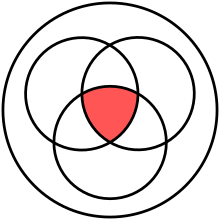
Venn diagram of

Notation
And is usually denoted by an infix operator: in mathematics and logic, it is denoted by ∧ , & or × ; in electronics, ⋅ ; and in programming languages,
&, &&, or and. In Jan Łukasiewicz's prefix notation for logic, the operator is K, for Polish koniunkcja.[1]Definition
Logical conjunction is an operation on two logical values, typically the values of two propositions, that produces a value of true if and only if both of its operands are true.
The conjunctive identity is 1, which is to say that AND-ing an expression with 1 will never change the value of the expression. In keeping with the concept of vacuous truth, when conjunction is defined as an operator or function of arbitrary arity, the empty conjunction (AND-ing over an empty set of operands) is often defined as having the result 1.
Truth table

The truth table of :
| T | T | T |
| T | F | F |
| F | T | F |
| F | F | F |

Defined by other operators
In systems where logical conjunction is not a primitive, it may be defined as[2]

Introduction and elimination rules
As a rule of inference, conjunction Introduction is a classically valid, simple argument form. The argument form has two premises, A and B. Intuitively, it permits the inference of their conjunction.
- A,
- B.
- Therefore, A and B.
or in logical operator notation:


Here is an example of an argument that fits the form conjunction introduction:
- Bob likes apples.
- Bob likes oranges.
- Therefore, Bob likes apples and oranges.
Conjunction elimination is another classically valid, simple argument form. Intuitively, it permits the inference from any conjunction of either element of that conjunction.
- A and B.
- Therefore, A.
...or alternately,
- A and B.
- Therefore, B.
In logical operator notation:

...or alternately,

Properties
commutativity: yes


associativity: yes
 |  |  |  |  |


distributivity: with various operations, especially with or
|  |  | |  |


| showothers |
|---|
idempotency: yes


monotonicity: yes
 |  | | |


truth-preserving: yes
When all inputs are true, the output is true.
When all inputs are true, the output is true.
| (to be tested) |
falsehood-preserving: yes
When all inputs are false, the output is false.
When all inputs are false, the output is false.
| (to be tested) |

Walsh spectrum: (1,-1,-1,1)
If using binary values for true (1) and false (0), then logical conjunction works exactly like normal arithmetic multiplication.
Applications in computer engineering

In high-level computer programming and digital electronics, logical conjunction is commonly represented by an infix operator, usually as a keyword such as "
AND", an algebraic multiplication, or the ampersand symbol "&". Many languages also provide short-circuit control structures corresponding to logical conjunction.
Logical conjunction is often used for bitwise operations, where
0 corresponds to false and 1 to true:0 AND 0=0,0 AND 1=0,1 AND 0=0,1 AND 1=1.
The operation can also be applied to two binary words viewed as bitstrings of equal length, by taking the bitwise AND of each pair of bits at corresponding positions. For example:
11000110 AND 10100011=10000010.
This can be used to select part of a bitstring using a bit mask. For example,
10011101 AND 00001000 = 00001000 extracts the fifth bit of an 8-bit bitstring.
In computer networking, bit masks are used to derive the network address of a subnet within an existing network from a given IP address, by ANDing the IP address and the subnet mask.
The Curry–Howard correspondence relates logical conjunction to product types.
Set-theoretic correspondence
The membership of an element of an intersection set in set theory is defined in terms of a logical conjunction: x ∈ A ∩ B if and only if (x ∈ A) ∧ (x ∈ B). Through this correspondence, set-theoretic intersection shares several properties with logical conjunction, such as associativity, commutativity, and idempotence.
Natural language
As with other notions formalized in mathematical logic, the logical conjunction and is related to, but not the same as, the grammatical conjunction and in natural languages.
English "and" has properties not captured by logical conjunction. For example, "and" sometimes implies order. For example, "They got married and had a child" in common discourse means that the marriage came before the child. The word "and" can also imply a partition of a thing into parts, as "The American flag is red, white, and blue." Here it is not meant that the flag is at once red, white, and blue, but rather that it has a part of each color.
Conjunction introduction (often abbreviated simply as conjunction and also called and introduction) is a valid rule of inference of propositional logic. The rule makes it possible to introduce a conjunction into a logical proof. It is the inference that if the proposition p is true, and proposition q is true, then the logical conjunction of the two propositions p and q is true. For example, if it's true that it's raining, and it's true that I'm inside, then it's true that "it's raining and I'm inside". The rule can be stated:

where the rule is that wherever an instance of "" and "" appear on lines of a proof, a "" can be placed on a subsequent line.


Formal notation
The conjunction introduction rule may be written in sequent notation:

where is a metalogical symbol meaning that is a syntactic consequence if and are each on lines of a proof in some logical system;

Conjunction elimination
In propositional logic, conjunction elimination (also called and elimination, ∧ elimination, or simplification) is a valid immediate inference, argument form and rule of inference which makes the inference that, if the conjunction A and B is true, then A is true, and B is true. The rule makes it possible to shorten longer proofs by deriving one of the conjuncts of a conjunction on a line by itself.
An example in English:
- It's raining and it's pouring.
- Therefore it's raining.
The rule consists of two separate sub-rules, which can be expressed in formal language as:

and

The two sub-rules together mean that, whenever an instance of "" appears on a line of a proof, either "" or "" can be placed on a subsequent line by itself. The above example in English is an application of the first sub-rule.
Formal notation
The conjunction elimination sub-rules may be written in sequent notation:

and

where is a metalogical symbol meaning that is a syntactic consequence of and is also a syntactic consequence of in logical system;
and expressed as truth-functional tautologies or theorems of propositional logic:

and

Logical graph
A logical graph is a special type of diagramatic structure in any one of several systems of graphical syntax that Charles Sanders Peirce developed for logic.
In his papers on qualitative logic, entitative graphs, and existential graphs, Peirce developed several versions of a graphical formalism, or a graph-theoretic formal language, designed to be interpreted for logic.
In the century since Peirce initiated this line of development, a variety of formal systems have branched out from what is abstractly the same formal base of graph-theoretic structures.
example :
Truth value
In logic and mathematics, a truth value, sometimes called a logical value, is a value indicating the relation of a proposition to truth .
Classical logic
⊤
true |
·∧·
conjunction | ||
¬
|
↕
|
↕
| |
⊥
false |
·∨·
disjunction | ||
| Negation interchanges true with false and conjunction with disjunction | |||
In classical logic, with its intended semantics, the truth values are true (1 or T), and untrue or false (0 or ⊥); that is, classical logic is a two-valued logic. This set of two values is also called the Boolean domain. Corresponding semantics of logical connectives are truth functions, whose values are expressed in the form of truth tables. Logical biconditional becomes the equality binary relation, and negation becomes a bijection which permutes true and false. Conjunction and disjunction are dual with respect to negation, which is expressed by De Morgan's laws:
- ¬(p∧q) ⇔ ¬p ∨ ¬q
- ¬(p∨q) ⇔ ¬p ∧ ¬q
Propositional variables become variables in the Boolean domain. Assigning values for propositional variables is referred to as valuation.
Intuitionistic and constructive logic
In intuitionistic logic, and more generally, constructive mathematics, statements are assigned a truth value only if they can be given a constructive proof. It starts with a set of axioms, and a statement is true if one can build a proof of the statement from those axioms. A statement is false if one can deduce a contradiction from it. This leaves open the possibility of statements that have not yet been assigned a truth value. Unproven statements in intuitionistic logic are not given an intermediate truth value (as is sometimes mistakenly asserted). Indeed, one can prove that they have no third truth value, a result dating back to Glivenko in 1928.[2]
Instead, statements simply remain of unknown truth value, until they are either proven or disproven.
There are various ways of interpreting intuitionistic logic, including the Brouwer–Heyting–Kolmogorov interpretation. See also Intuitionistic logic#Semantics.
Multi-valued logic
Multi-valued logics (such as fuzzy logic and relevance logic) allow for more than two truth values, possibly containing some internal structure. For example, on the unit interval [0,1] such structure is a total order; this may be expressed as the existence of various degrees of truth.
Algebraic semantics
Not all logical systems are truth-valuational in the sense that logical connectives may be interpreted as truth functions. For example, intuitionistic logic lacks a complete set of truth values because its semantics, the Brouwer–Heyting–Kolmogorov interpretation, is specified in terms of provability conditions, and not directly in terms of the necessary truth of formulae.
But even non-truth-valuational logics can associate values with logical formulae, as is done in algebraic semantics. The algebraic semantics of intuitionistic logic is given in terms of Heyting algebras, compared to Boolean algebra semantics of classical propositional calculus.
In other theories
Intuitionistic type theory uses types in the place of truth values.
Topos theory uses truth values in a special sense: the truth values of a topos are the global elements of the subobject classifier. Having truth values in this sense does not make a logic truth valuational.
Operation (mathematics)
In mathematics, an operation is a calculation from zero or more input values (called operands) to an output value. The number of operands is the arity of the operation. The most commonly studied operations are binary operations, (that is, operations of arity 2) such as addition and multiplication, and unary operations (operations of arity 1), such as additive inverse and multiplicative inverse. An operation of arity zero, or nullary operation, is a constant. The mixed product is an example of an operation of arity 3, also called ternary operation. Generally, the arity is supposed to be finite. However, infinitary operations are sometimes considered, in which context the "usual" operations of finite arity are called finitary operations.

- +, plus (addition)
- −, minus (subtraction)
- ÷, obelus (division)
- ×, times (multiplication)
Types of operation


There are two common types of operations: unary and binary. Unary operations involve only one value, such as negation and trigonometric functions. Binary operations, on the other hand, take two values, and include addition, subtraction, multiplication, division, and exponentiation.
Operations can involve mathematical objects other than numbers. The logical values true and false can be combined using logic operations, such as and, or, and not. Vectors can be added and subtracted. Rotations can be combined using the function composition operation, performing the first rotation and then the second. Operations on sets include the binary operations union and intersection and the unary operation of complementation. Operations on functions include composition and convolution.
Operations may not be defined for every possible value. For example, in the real numbers one cannot divide by zero or take square roots of negative numbers. The values for which an operation is defined form a set called its domain. The set which contains the values produced is called the codomain, but the set of actual values attained by the operation is its range. For example, in the real numbers, the squaring operation only produces non-negative numbers; the codomain is the set of real numbers, but the range is the non-negative numbers.
Operations can involve dissimilar objects. A vector can be multiplied by a scalar to form another vector. And the inner product operation on two vectors produces a scalar. An operation may or may not have certain properties, for example it may be associative, commutative, anticommutative, idempotent, and so on.
The values combined are called operands, arguments, or inputs, and the value produced is called the value, result, or output. Operations can have fewer or more than two inputs.
An operation is like an operator, but the point of view is different. For instance, one often speaks of "the operation of addition" or "addition operation" when focusing on the operands and result, but one says "addition operator" (rarely "operator of addition") when focusing on the process, or from the more abstract viewpoint, the function + : S × S → S.
General description
An operation ω is a function of the form ω : V → Y, where V ⊂ X1 × ... × Xk. The sets Xk are called the domains of the operation, the set Y is called the codomain of the operation, and the fixed non-negative integer k (the number of arguments) is called the type or arity of the operation. Thus a unary operation has arity one, and a binary operation has arity two. An operation of arity zero, called a nullary operation, is simply an element of the codomain Y. An operation of arity k is called a k-ary operation. Thus a k-ary operation is a (k+1)-ary relation that is functional on its first k domains.
The above describes what is usually called a finitary operation, referring to the finite number of arguments (the value k). There are obvious extensions where the arity is taken to be an infinite ordinal or cardinal, or even an arbitrary set indexing the arguments.
Often, use of the term operation implies that the domain of the function is a power of the codomain (i.e. the Cartesian product of one or more copies of the codomain),[1] although this is by no means universal, as in the example of multiplying a vector by a scalar.
Hyperoperation
In mathematics, the hyperoperation sequence[nb 1] is an infinite sequence of arithmetic operations (called hyperoperations) that starts with the unary operation of successor (n = 0), then continues with the binary operations of addition (n = 1), multiplication (n = 2), and exponentiation (n = 3), after which the sequence proceeds with further binary operations extending beyond exponentiation, using right-associativity. For the operations beyond exponentiation, the nth member of this sequence is named by Reuben Goodstein after the Greek prefix of n suffixed with -ation (such as tetration (n = 4), pentation (n = 5), hexation (n = 6), etc.)[5] and can be written as using n − 2 arrows in Knuth's up-arrow notation. Each hyperoperation may be understood recursively in terms of the previous one by:
![{\displaystyle a[n]b=\underbrace {a[n-1](a[n-1](a[n-1](\cdots [n-1](a[n-1](a[n-1]a))\cdots )))} _{\displaystyle b{\mbox{ copies of }}a},\quad n\geq 2}](https://wikimedia.org/api/rest_v1/media/math/render/svg/2b5b37b38e6798ec67d72e429a051aa7641fb571)
It may also be defined according to the recursion rule part of the definition, as in Knuth's up-arrow version of the Ackermann function:
![{\displaystyle a[n]b=a[n-1]\left(a[n]\left(b-1\right)\right),\quad n\geq 1}](https://wikimedia.org/api/rest_v1/media/math/render/svg/acfe8d681527fde64d3bcacced77270f96900f25)
This can be used to easily show numbers much larger than those which scientific notation can, such as Skewes' number and googolplexplex (e.g. is much larger than Skewes’ number and googolplexplex), but there are some numbers which even they cannot easily show, such as Graham's number and TREE(3).
![{\displaystyle 50[50]50}](https://wikimedia.org/api/rest_v1/media/math/render/svg/e849d9d2bf3c592596ad3b7670cb605f68ccf252)
This recursion rule is common to many variants of hyperoperations .
Definition


![{\displaystyle H_{n}(a,b)=a[n]b={\begin{cases}b+1&{\text{if }}n=0\\a&{\text{if }}n=1{\text{ and }}b=0\\0&{\text{if }}n=2{\text{ and }}b=0\\1&{\text{if }}n\geq 3{\text{ and }}b=0\\H_{n-1}(a,H_{n}(a,b-1))&{\text{otherwise}}\end{cases}}}](https://wikimedia.org/api/rest_v1/media/math/render/svg/d09394c6d619461dc93752b66df45b661a32a4cb)
(Note that for n = 0, the binary operation essentially reduces to a unary operation (successor function) by ignoring the first argument.)
For n = 0, 1, 2, 3, this definition reproduces the basic arithmetic operations of successor (which is a unary operation), addition, multiplication, and exponentiation, respectively, as

So what will be the next operation after exponentiation? We defined multiplication so that , and defined exponentiation so that so it seems logical to define the next operation, tetration, so that with a tower of three 'a'. Analogously, the pentation of (a, 3) will be tetration(a, tetration(a, a)), with three "a" in it.
![{\displaystyle H_{2}(a,3)=a[2]3=a\times 3=a+a+a,}](https://wikimedia.org/api/rest_v1/media/math/render/svg/83c8d39f8da198f717d8981669109e55dca411cc)
![{\displaystyle H_{3}(a,3)=a[3]3=a^{3}=a\cdot a\cdot a,}](https://wikimedia.org/api/rest_v1/media/math/render/svg/e099408ee3d045c50580281b76add357b53a8e01)
![{\displaystyle H_{4}(a,3)=a[4]3=\operatorname {tetration} (a,3)=a^{a^{a}},}](https://wikimedia.org/api/rest_v1/media/math/render/svg/1598365465790ae769ba5993e70a525bd72dcf71)
The H operations for n ≥ 3 can be written in Knuth's up-arrow notation as

Knuth's notation could be extended to negative indices ≥ −2 in such a way as to agree with the entire hyperoperation sequence, except for the lag in the indexing:

The hyperoperations can thus be seen as an answer to the question "what's next" in the sequence: successor, addition, multiplication, exponentiation, and so on. Noting that
![{\displaystyle {\begin{aligned}a+b&=(a+(b-1))+1\\a\cdot b&=a+(a\cdot (b-1))\\a^{b}&=a\cdot \left(a^{(b-1)}\right)\\a[4]b&=a^{a[4](b-1)}\end{aligned}}}](https://wikimedia.org/api/rest_v1/media/math/render/svg/fe5adbfca7ba2ea5ef0116db091a9fdd09f6bff1)
the relationship between basic arithmetic operations is illustrated, allowing the higher operations to be defined naturally as above. The parameters of the hyperoperation hierarchy are sometimes referred to by their analogous exponentiation term;[14] so a is the base, b is the exponent (or hyperexponent),[12] and n is the rank (or grade).[6], and is read as "the bth n-ation of a", e.g. is read as "the 9th tetration of 7", and is read as "the 789th 123-ation of 456".


In common terms, the hyperoperations are ways of compounding numbers that increase in growth based on the iteration of the previous hyperoperation. The concepts of successor, addition, multiplication and exponentiation are all hyperoperations; the successor operation (producing x + 1 from x) is the most primitive, the addition operator specifies the number of times 1 is to be added to itself to produce a final value, multiplication specifies the number of times a number is to be added to itself, and exponentiation refers to the number of times a number is to be multiplied by itself.
Examples
Below is a list of the first seven (0th to 6th) hyperoperations (0⁰ is defined as 1.).
| n | Operation, Hn(a, b) | Definition | Names | Domain |
|---|---|---|---|---|
| 0 | or | hyper0, increment, successor, zeration | Arbitrary | |
| 1 | or | hyper1, addition | Arbitrary | |
| 2 | or | hyper2, multiplication | Arbitrary | |
| 3 | or | hyper3, exponentiation | b real, with some multivalued extensions to complex numbers | |
| 4 | or | hyper4, tetration | a ≥ 0 or an integer, b an integer ≥ −1[nb 2] (with some proposed extensions) | |
| 5 | hyper5, pentation | a, b integers ≥ −1[nb 2] | ||
| 6 | hyper6, hexation | a, b integers ≥ −1[nb 2] |

![{\displaystyle a[0]b}](https://wikimedia.org/api/rest_v1/media/math/render/svg/8e33bf19ab5a8ade49e2e4faad2899d7bd35bc5e)


![{\displaystyle a[1]b}](https://wikimedia.org/api/rest_v1/media/math/render/svg/ea88ed1e0ba5cc1204e06635803d66a81cab90ed)


![{\displaystyle a[2]b}](https://wikimedia.org/api/rest_v1/media/math/render/svg/6761632b308609eeaf05407389355d3a98758c6f)


![{\displaystyle a[3]b}](https://wikimedia.org/api/rest_v1/media/math/render/svg/dd946603b3dd3c072053d13fbe120d44f70ac8ab)


![{\displaystyle a[4]b}](https://wikimedia.org/api/rest_v1/media/math/render/svg/dfddc8a9d38692fe9ac6ecee1527c90dd2ecccca)
)\cdots )))} _{\displaystyle b{\mbox{ copies of }}a}}](https://wikimedia.org/api/rest_v1/media/math/render/svg/3612774b867e26b11d0e4653952cadba81128e4b)
![{\displaystyle a[5]b}](https://wikimedia.org/api/rest_v1/media/math/render/svg/d782af460e582816fb4e49d3907b621dd297d4d3)
)\cdots )))} _{\displaystyle b{\mbox{ copies of }}a}}](https://wikimedia.org/api/rest_v1/media/math/render/svg/ae8020b2baedd1415289038c096c179cccb37794)
![{\displaystyle a[6]b}](https://wikimedia.org/api/rest_v1/media/math/render/svg/440cac430b226ebceafac2548525b7f1aef2486c)
)\cdots )))} _{\displaystyle b{\mbox{ copies of }}a}}](https://wikimedia.org/api/rest_v1/media/math/render/svg/8c85d0f485080c5075bc3918b09c9df863e5b3c0)
Special cases
Hn(0, b) =
- 0, when n = 2, or n = 3, b ≥ 1, or n ≥ 4, b odd (≥ −1)
- 1, when n = 3, b = 0, or n ≥ 4, b even (≥ 0)
- b, when n = 1
- b + 1, when n = 0
Hn(1, b) =
- 1, when n ≥ 3
Hn(a, 0) =
- 0, when n = 2
- 1, when n = 0, or n ≥ 3
- a, when n = 1
Hn(a, 1) =
- a, when n ≥ 2
Hn(a, −1) =[nb 2]
- 0, when n = 0, or n ≥ 4
- a − 1, when n = 1
- −a, when n = 2
- 1a , when n = 3
Hn(2, 2) =
- 3, when n = 0
- 4, when n ≥ 1, easily demonstrable recursively.
Flash Back
One of the earliest discussions of hyperoperations was that of Albert Bennett[6] in 1914, who developed some of the theory of commutative hyperoperations (see below). About 12 years later, Wilhelm Ackermann defined the function [15] which somewhat resembles the hyperoperation sequence.

In his 1947 paper,[5] R. L. Goodstein introduced the specific sequence of operations that are now called hyperoperations, and also suggested the Greek names tetration, pentation, etc., for the extended operations beyond exponentiation (because they correspond to the indices 4, 5, etc.). As a three-argument function, e.g., , the hyperoperation sequence as a whole is seen to be a version of the original Ackermann function — recursive but not primitive recursive — as modified by Goodstein to incorporate the primitive successor function together with the other three basic operations of arithmetic (addition, multiplication, exponentiation), and to make a more seamless extension of these beyond exponentiation.

The original three-argument Ackermann function uses the same recursion rule as does Goodstein's version of it (i.e., the hyperoperation sequence), but differs from it in two ways. First, defines a sequence of operations starting from addition (n = 0) rather than the successor function, then multiplication (n = 1), exponentiation (n = 2), etc. Secondly, the initial conditions for result in , thus differing from the hyperoperations beyond exponentiation. The significance of the b + 1 in the previous expression is that = , where b counts the number of operators (exponentiations), rather than counting the number of operands ("a"s) as does the b in , and so on for the higher-level operations. (See the Ackermann function article for details.)

}](https://wikimedia.org/api/rest_v1/media/math/render/svg/3467af278839156bdfbae125af0a32d18cd902d6)


Notations
This is a list of notations that have been used for hyperoperations.
| Name | Notation equivalent to | Comment |
|---|---|---|
| Knuth's up-arrow notation | Used by Knuth[18] (for n ≥ 3), and found in several reference books. | |
| Goodstein's notation | Used by Reuben Goodstein.[5] | |
| Original Ackermann function | Used by Wilhelm Ackermann (for n ≥ 1)[15] | |
| Ackermann–Péter function | This corresponds to hyperoperations for base 2 (a = 2) | |
| Nambiar's notation | Used by Nambiar (for n ≥ 1)[21] | |
| Box notation | Used by Rubtsov and Romerio. | |
| Superscript notation | Used by Robert Munafo.[10] | |
| Subscript notation (for lower hyperoperations) | Used for lower hyperoperations by Robert Munafo. | |
| Operator notation (for "extended operations") | Used for lower hyperoperations by John Donner and Alfred Tarski (for n ≥ 1). | |
| Square bracket notation | Used in many online forums; convenient for ASCII. | |
| Conway chained arrow notation | Used by John Horton Conway (for n ≥ 3) | |
| Bowers' Exploding Array Function | Used by Jonathan Bowers (for n ≥ 1) |


![{\displaystyle a[n]b}](https://wikimedia.org/api/rest_v1/media/math/render/svg/2551ef8c0122ea93c537b613b561246ca3f8724f)


Variant starting from a
In 1928, Wilhelm Ackermann defined a 3-argument function which gradually evolved into a 2-argument function known as the Ackermann function. The original Ackermann function was less similar to modern hyperoperations, because his initial conditions start with for all n > 2. Also he assigned addition to n = 0, multiplication to n = 1 and exponentiation to n = 2, so the initial conditions produce very different operations for tetration and beyond.

| n | Operation | Comment |
|---|---|---|
| 0 | ||
| 1 | ||
| 2 | ||
| 3 | An offset form of tetration. The iteration of this operation is different than the iteration of tetration. | |
| 4 | Not to be confused with pentation. |


}](https://wikimedia.org/api/rest_v1/media/math/render/svg/c4cd80f3850f8a52ab3a1b23acba831f7148e692)
)^{b}(a)}](https://wikimedia.org/api/rest_v1/media/math/render/svg/f27ed90acc3f9f63d6c22be4366b0f3def9ea920)
Another initial condition that has been used is (where the base is constant ), due to Rózsa Péter, which does not form a hyperoperation hierarchy.


Variant starting from 0
In 1984, C. W. Clenshaw and F. W. J. Olver began the discussion of using hyperoperations to prevent computer floating-point overflows. Since then, many other authors have renewed interest in the application of hyperoperations to floating-point representation. (Since Hn(a, b) are all defined for b = -1.) While discussing tetration, Clenshaw et al. assumed the initial condition , which makes yet another hyperoperation hierarchy. Just like in the previous variant, the fourth operation is very similar to tetration, but offset by one.

| n | Operation | Comment |
|---|---|---|
| 0 | ||
| 1 | ||
| 2 | ||
| 3 | ||
| 4 | An offset form of tetration. The iteration of this operation is much different than the iteration of tetration. | |
| 5 | Not to be confused with pentation. |


}](https://wikimedia.org/api/rest_v1/media/math/render/svg/488ccddf037f628486ad2255768e6ddeb327ff23)
\right)^{b}(0)=0{\text{ if }}a>0}](https://wikimedia.org/api/rest_v1/media/math/render/svg/96070b5541117aec6f43b67bc3269f9e8933f1f4)
Lower hyperoperations
An alternative for these hyperoperations is obtained by evaluation from left to right. Since

define (with ° or subscript)

with

This was extended to ordinal numbers by Donner and Tarski,[22][Definition 1] by :

It follows from Definition 1(i), Corollary 2(ii), and Theorem 9, that, for a ≥ 2 and b ≥ 1, that[original research?]

But this suffers a kind of collapse, failing to form the "power tower" traditionally expected of hyperoperators:[22][Theorem 3(iii)][nb 3]


| n | Operation | Comment |
|---|---|---|
| 0 | increment, successor, zeration | |
| 1 | ||
| 2 | ||
| 3 | This is exponentiation. | |
| 4 | Not to be confused with tetration. | |
| 5 | Not to be confused with pentation. Similar to tetration. |


Commutative hyperoperations
Commutative hyperoperations were considered by Albert Bennett as early as 1914, which is possibly the earliest remark about any hyperoperation sequence. Commutative hyperoperations are defined by the recursion rule

which is symmetric in a and b, meaning all hyperoperations are commutative. This sequence does not contain exponentiation, and so does not form a hyperoperation hierarchy.
| n | Operation | Comment |
|---|---|---|
| 0 | ||
| 1 | ||
| 2 | This is due to the properties of the logarithm. | |
| 3 | A commutative form of exponentiation. | |
| 4 | Not to be confused with tetration. |


Order of operations
In mathematics and computer programming, the order of operations (or operator precedence) is a collection of rules that reflect conventions about which procedures to perform first in order to evaluate a given mathematical expression.
For example, in mathematics and most computer languages, multiplication is granted a higher precedence than addition, and it has been this way since the introduction of modern algebraic notation.[1][2] Thus, the expression 2 + 3 × 4 is interpreted to have the value 2 + (3 × 4) = 14, not (2 + 3) × 4 = 20. With the introduction of exponents in the 16th and 17th centuries, they were given precedence over both addition and multiplication and could be placed only as a superscript to the right of their base.[1] Thus 3 + 52 = 28 and 3 × 52 = 75.
These conventions exist to eliminate ambiguity while allowing notation to be as brief as possible. Where it is desired to override the precedence conventions, or even simply to emphasize them, parentheses ( ) (sometimes replaced by brackets [ ] or braces { } for readability) can indicate an alternate order or reinforce the default order to avoid confusion. For example, (2 + 3) × 4 = 20 forces addition to precede multiplication, and (3 + 5)2 = 64 forces addition to precede exponentiation.
Definition
The order of operations used throughout mathematics, science, technology and many computer programming languages is expressed here:
This means that if a mathematical expression is preceded by one binary operator and followed by another, the operator higher on the list should be applied first.[1]
The commutative and associative laws of addition and multiplication allow adding terms in any order, and multiplying factors in any order—but mixed operations must obey the standard order of operations.
It is helpful[clarification needed] to treat division as multiplication by the reciprocal (multiplicative inverse) and subtraction as addition of the opposite (additive inverse).[citation needed] Thus 3 ÷ 4 = 3 × ¼; in other words the quotient of 3 and 4 equals the product of 3 and ¼. Also 3 − 4 = 3 + (−4); in other words the difference of 3 and 4 equals the sum of 3 and −4. Thus, 1 − 3 + 7 can be thought of as the sum of 1, −3, and 7, and add in any order: (1 − 3) + 7 = −2 + 7 = 5 and in reverse order (7 − 3) + 1 = 4 + 1 = 5, always keeping the negative sign with the 3.
The root symbol √ requires a symbol of grouping around the radicand. The usual symbol of grouping is a bar (called vinculum) over the radicand. Other functions use parentheses around the input to avoid ambiguity. The parentheses are sometimes omitted if the input is a monomial. Thus, sin 3x = sin(3x), but sin x + y = sin(x) + y, because x + y is not a monomial.[1] Some calculators and programming languages require parentheses around function inputs, some do not.
Symbols of grouping can be used to override the usual order of operations.[1] Grouped symbols can be treated as a single expression.[1] Symbols of grouping can be removed using the associative and distributive laws, also they can be removed if the expression inside the symbol of grouping is sufficiently simplified so no ambiguity results from their removal.
Examples

A horizontal fractional line also acts as a symbol of grouping:

For ease in reading, other grouping symbols, such as curly braces { } or square brackets [ ], are often used along with parentheses ( ). For example:
![{\displaystyle [(1+2)-3]-(4-5)=[3-3]-(-1)=1.}](https://wikimedia.org/api/rest_v1/media/math/render/svg/491249623dd91c5e6b2aa952d3e43c42877e8ccf)
Exceptions
Unary minus sign
There are differing conventions concerning the unary operator − (usually read "minus"). In written or printed mathematics, the expression −32 is interpreted to mean 0 − (32) = − 9,[1][4]
Some applications and programming languages, notably Microsoft Excel (and other spreadsheet applications) and the programming language bc, unary operators have a higher priority than binary operators, that is, the unary minus has higher precedence than exponentiation, so in those languages −32 will be interpreted as (−3)2 = 9.[5] This does not apply to the binary minus operator −; for example while the formulas
=-2^2 and =0+-2^2 return 4 in Microsoft Excel, the formula =0-2^2 returns −4. In cases where there is the possibility that the notation might be misinterpreted, a binary minus operation can be enforced by explicitly specifying a leading 0 (as in 0-2^2 instead of just -2^2), or parentheses can be used to clarify the intended meaning.Mixed division and multiplication
Similarly, there can be ambiguity in the use of the slash symbol / in expressions such as 1/2x.[6] If one rewrites this expression as 1 ÷ 2x and then interprets the division symbol as indicating multiplication by the reciprocal, this becomes:
- 1 ÷ 2 × x = 1 × ½ × x = ½ × x.
With this interpretation 1 ÷ 2x is equal to (1 ÷ 2)x.[1][7] However, in some of the academic literature, multiplication denoted by juxtaposition (also known as implied multiplication) is interpreted as having higher precedence than division, so that 1 ÷ 2x equals 1 ÷ (2x), not (1 ÷ 2)x.
For example, the manuscript submission instructions for the Physical Review journals state that multiplication is of higher precedence than division with a slash,[8] and this is also the convention observed in prominent physics textbooks such as the Course of Theoretical Physics by Landau and Lifshitz and the Feynman Lectures on Physics.[a]
Mnemonics
Mnemonics are often used to help students remember the rules, involving the first letters of words representing various operations. Different mnemonics are in use in different countries.[9][10][11]
- In the United States, the acronym PEMDAS is common. It stands for Parentheses, Exponents, Multiplication/Division, Addition/Subtraction. PEMDAS is often expanded to the mnemonic "Please Excuse My Dear Aunt Sally".[6]
- Canada and New Zealand use BEDMAS, standing for Brackets, Exponents, Division/Multiplication, Addition/Subtraction.
- Most common in the UK, India and Australia[12] are BODMAS meaning Brackets, Order, Division/Multiplication, Addition/Subtraction. Nigeria and some other West African countries also use BODMAS. Similarly in the UK, BIDMAS is used, standing for Brackets, Indices, Division/Multiplication, Addition/Subtraction.
These mnemonics may be misleading when written this way.[6] For example, misinterpreting any of the above rules to mean "addition first, subtraction afterward" would incorrectly evaluate the expression[6]
- 10 − 3 + 2.
The correct value is 9 (and not 5, as if the addition would be carried out first and the result used with the subtraction afterwards).
Special cases
Serial exponentiation
If exponentiation is indicated by stacked symbols, the usual rule is to work from the top down, because exponentiation is right-associative in mathematics thus:
- abc = a(bc)
which typically is not equal to (ab)c.
However, some computer systems may resolve the ambiguous expression differently.[14] For example, Microsoft Excel evaluates
a^b^c as (ab)c, which is opposite of normally accepted convention of top-down order of execution for exponentiation. Thus 4^3^2 is evaluated to 4,096 instead of 262,144.
Another difference in Microsoft Excel is
-a^b which is evaluated as (-a)^b instead of -(a^b). For compatibility, the same behavior is observed on LibreOffice. The computational programming language MATLAB is another example of a computer system resolving the stacked exponentiation in the non-standard way.Serial division
A similar ambiguity exists in the case of serial division, for example, the expression 10 ÷ 5 ÷ 2 can either be interpreted as
- 10 ÷ ( 5 ÷ 2 ) = 4
or as
- ( 10 ÷ 5 ) ÷ 2 = 1
The left-to-right operation convention would resolve the ambiguity in favor of the last expression. Further, the mathematical habit of combining factors and representing division as multiplication by a reciprocal both greatly reduce the frequency of ambiguous division. However, when two long expressions are combined by division, the correct order of operations can be lost in the notation.
Calculators
Different calculators follow different orders of operations. Many simple calculators without a stack implement chain input working left to right without any priority given to different operators, for example typing
1 + 2 × 3yields 9,
while more sophisticated calculators will use a more standard priority, for example typing
1 + 2 × 3yields 7.
The Microsoft Calculator program uses the former in its standard view and the latter in its scientific and programmer views.
Chain input expects two operands and an operator. When the next operator is pressed, the expression is immediately evaluated and the answer becomes the left hand of the next operator. Advanced calculators allow entry of the whole expression, grouped as necessary, and evaluates only when the user uses the equals sign.
Calculators may associate exponents to the left or to the right depending on the model or the evaluation mode. For example, the expression
a^b^c is interpreted as a(bc) on the TI-92 and the TI-30XS MultiView in "Mathprint mode", whereas it is interpreted as (ab)con the TI-30XII and the TI-30XS MultiView in "Classic mode".
An expression like
1/2x is interpreted as 1/(2x) by TI-82, but as (1/2)x by TI-83 and every other TI calculator released since 1996,[15] as well as by all Hewlett-Packard calculators with algebraic notation. While the first interpretation may be expected by some users, only the latter is in agreement with the standard rule that multiplication and division are of equal precedence, so 1/2x is read one divided by two and the answer multiplied by x.
When the user is unsure how a calculator will interpret an expression, it is a good idea to use parentheses so there is no ambiguity.
Calculators that utilize reverse Polish notation (RPN), also known as postfix notation, use a stack to enter formulas without the need for parentheses.[6]
Programming languages
Some programming languages use precedence levels that conform to the order commonly used in mathematics,[14] though others, such as APL, Smalltalk or Occam, have no operator precedence rules (in APL, evaluation is strictly right to left; in Smalltalk and Occam, it is strictly left to right).
In addition, because many operators are not associative, the order within any single level is usually defined by grouping left to right so that
16/4/4 is interpreted as (16/4)/4 = 1 rather than 16/(4/4) = 16; such operators are perhaps misleadingly referred to as "left associative". Exceptions exist; for example, languages with operators corresponding to the cons operation on lists usually make them group right to left ("right associative"), e.g. in Haskell, 1:2:3:4:[] == 1:(2:(3:(4:[]))) == [1,2,3,4].
The logical bitwise operators in C (and all programming languages that borrow precedence rules from C, for example, C++, Perl and PHP) have a precedence level that the creator of the C language considered unsatisfactory.[18] However, many programmers have become accustomed to this order. The relative precedence levels of operators found in many C-style languages are as follows:
| 1 | () [] -> . :: | Function call, scope, array/member access |
| 2 | ! ~ - + * & sizeof type cast ++ -- | (most) unary operators, sizeof and type casts (right to left) |
| 3 | * / % MOD | Multiplication, division, modulo |
| 4 | + - | Addition and subtraction |
| 5 | << >> | Bitwise shift left and right |
| 6 | < <= > >= | Comparisons: less-than and greater-than |
| 7 | == != | Comparisons: equal and not equal |
| 8 | & | Bitwise AND |
| 9 | ^ | Bitwise exclusive OR (XOR) |
| 10 | | | Bitwise inclusive (normal) OR |
| 11 | && | Logical AND |
| 12 | || | Logical OR |
| 13 | ? : | Conditional expression (ternary) |
| 14 | = += -= *= /= %= &= |= ^= <<= >>= | Assignment operators (right to left) |
| 15 | , | Comma operator |
Examples: (Note: in the examples below, '≡' is used to mean "is equivalent to", and not to be interpreted as an actual assignment operator used as part of the example expression.)
!A + !B≡(!A) + (!B)++A + !B≡(++A) + (!B)A + B * C≡A + (B * C)A || B && C≡A || (B && C)A && B == C≡A && (B == C)A & B == C≡A & (B == C)
Source-to-source compilers that compile to multiple languages need to explicitly deal with the issue of different order of operations across languages. Haxe for example standardizes the order and enforces it by inserting brackets where it is appropriate.
The accuracy of software developer knowledge about binary operator precedence has been found to closely follow their frequency of occurrence in source code
Propositional calculus
Propositional calculus is a branch of logic. It is also called propositional logic, statement logic, sentential calculus, sentential logic, or sometimes zeroth-order logic. It deals with propositions (which can be true or false) and argument flow. Compound propositions are formed by connecting propositions by logical connectives. The propositions without logical connectives are called atomic propositions. Unlike first-order logic, propositional logic does not deal with non-logical objects, predicates about them, or quantifiers. However, all the machinery of propositional logic is included in first-order logic and higher-order logics. In this sense, propositional logic is the foundation of first-order logic and higher-order logic.
Explanation
Logical connectives are found in natural languages. In English for example, some examples are "and" (conjunction), "or" (disjunction), "not” (negation) and "if" (but only when used to denote material conditional).
The following is an example of a very simple inference within the scope of propositional logic:
- Premise 1: If it's raining then it's cloudy.
- Premise 2: It's raining.
- Conclusion: It's cloudy.
Both premises and the conclusion are propositions. The premises are taken for granted and then with the application of modus ponens (an inference rule) the conclusion follows.
As propositional logic is not concerned with the structure of propositions beyond the point where they can't be decomposed anymore by logical connectives, this inference can be restated replacing those atomic statements with statement letters, which are interpreted as variables representing statements:
- Premise 1:
- Premise 2:
- Conclusion:

The same can be stated succinctly in the following way:

When P is interpreted as “It's raining” and Q as “it's cloudy” the above symbolic expressions can be seen to exactly correspond with the original expression in natural language. Not only that, but they will also correspond with any other inference of this form, which will be valid on the same basis that this inference is.
Propositional logic may be studied through a formal system in which formulas of a formal language may be interpreted to represent propositions. A system of inference rules and axioms allows certain formulas to be derived. These derived formulas are called theorems and may be interpreted to be true propositions. A constructed sequence of such formulas is known as a derivation or proof and the last formula of the sequence is the theorem. The derivation may be interpreted as proof of the proposition represented by the theorem.
When a formal system is used to represent formal logic, only statement letters are represented directly. The natural language propositions that arise when they're interpreted are outside the scope of the system, and the relation between the formal system and its interpretation is likewise outside the formal system itself.
Usually in truth-functional propositional logic, formulas are interpreted as having either a truth value of true or a truth value of false.[clarification needed] Truth-functional propositional logic and systems isomorphic to it, are considered to be zeroth-order logic.
XO__XO Digital Electronics for Microprocessor Applications in Control of Manufacturing Processes
The rapid development of microprocessor devices invites the industrial engineer to consider using microprocessors to solve data acquisition, machine control, and process control problems in ways that previously would have been apriori uneconomic. The initial simplicity of the microprocessor is often lost when the engineer finds that microprocessors are usually embedded in conventional digital electronic circuits. Fortunately, only a small class of digital electronic devices serves a variety of functions. When their operation and application is understood on a functional basis, the original simplicity of the microprocessor is largely retained. The suppliers of microprocessor products provide not only the microprocessor itself but also a wide range of supporting “chips” which allow the user to realize a microcomputer system of considerable power and flexibility. Nevertheless, the user usually finds a need to understand and use more conventional digital electronic circuits in conjunction with the microprocessor and its supporting devices.
Electrical Symbols & Electronic Symbols
Electrical symbols and electronic circuit symbols are used for drawing schematic diagram.
The symbols represent electrical and electronic components.
Table of Electrical Symbols
| Symbol | Component name | Meaning |
|---|---|---|
| Wire Symbols | ||
| Electrical Wire | Conductor of electrical current | |
| Connected Wires | Connected crossing | |
| Not Connected Wires | Wires are not connected | |
| Switch Symbols and Relay Symbols | ||
| SPST Toggle Switch | Disconnects current when open | |
| SPDT Toggle Switch | Selects between two connections | |
| Pushbutton Switch (N.O) | Momentary switch - normally open | |
| Pushbutton Switch (N.C) | Momentary switch - normally closed | |
| DIP Switch | DIP switch is used for onboard configuration | |
| SPST Relay | Relay open / close connection by an electromagnet | |
| SPDT Relay | ||
| Jumper | Close connection by jumper insertion on pins. | |
| Solder Bridge | Solder to close connection | |
| Ground Symbols | ||
| Earth Ground | Used for zero potential reference and electrical shock protection. | |
| Chassis Ground | Connected to the chassis of the circuit | |
| Digital / Common Ground | ||
| Resistor Symbols | ||
| Resistor (IEEE) | Resistor reduces the current flow. | |
| Resistor (IEC) | ||
| Potentiometer (IEEE) | Adjustable resistor - has 3 terminals. | |
| Potentiometer (IEC) | ||
| Variable Resistor / Rheostat (IEEE) | Adjustable resistor - has 2 terminals. | |
| Variable Resistor / Rheostat (IEC) | ||
| Trimmer Resistor | Preset resistor | |
| Thermistor | Thermal resistor - change resistance when temperature changes | |
| Photoresistor / Light dependent resistor (LDR) | Photo-resistor - change resistance with light intensity change | |
| Capacitor Symbols | ||
| Capacitor | Capacitor is used to store electric charge. It acts as short circuit with AC and open circuit with DC. | |
| Capacitor | ||
| Polarized Capacitor | Electrolytic capacitor | |
| Polarized Capacitor | Electrolytic capacitor | |
| Variable Capacitor | Adjustable capacitance | |
| Inductor / Coil Symbols | ||
| Inductor | Coil / solenoid that generates magnetic field | |
| Iron Core Inductor | Includes iron | |
| Variable Inductor | ||
| Power Supply Symbols | ||
| Voltage Source | Generates constant voltage | |
| Current Source | Generates constant current. | |
| AC Voltage Source | AC voltage source | |
| Generator | Electrical voltage is generated by mechanical rotation of the generator | |
| Battery Cell | Generates constant voltage | |
| Battery | Generates constant voltage | |
| Controlled Voltage Source | Generates voltage as a function of voltage or current of other circuit element. | |
| Controlled Current Source | Generates current as a function of voltage or current of other circuit element. | |
| Meter Symbols | ||
| Voltmeter | Measures voltage. Has very high resistance. Connected in parallel. | |
| Ammeter | Measures electric current. Has near zero resistance. Connected serially. | |
| Ohmmeter | Measures resistance | |
| Wattmeter | Measures electric power | |
| Lamp / Light Bulb Symbols | ||
| Lamp / light bulb | Generates light when current flows through | |
| Lamp / light bulb | ||
| Lamp / light bulb | ||
| Diode / LED Symbols | ||
| Diode | Diode allows current flow in one direction only - left (anode) to right (cathode). | |
| Zener Diode | Allows current flow in one direction, but also can flow in the reverse direction when above breakdown voltage | |
| Schottky Diode | Schottky diode is a diode with low voltage drop | |
| Varactor / Varicap Diode | Variable capacitance diode | |
| Tunnel Diode | ||
| Light Emitting Diode (LED) | LED emits light when current flows through | |
| Photodiode | Photodiode allows current flow when exposed to light | |
| Transistor Symbols | ||
| NPN Bipolar Transistor | Allows current flow when high potential at base (middle) | |
| PNP Bipolar Transistor | Allows current flow when low potential at base (middle) | |
| Darlington Transistor | Made from 2 bipolar transistors. Has total gain of the product of each gain. | |
| JFET-N Transistor | N-channel field effect transistor | |
| JFET-P Transistor | P-channel field effect transistor | |
| NMOS Transistor | N-channel MOSFET transistor | |
| PMOS Transistor | P-channel MOSFET transistor | |
| Misc. Symbols | ||
| Motor | Electric motor | |
| Transformer | Change AC voltage from high to low or low to high. | |
| Electric bell | Rings when activated | |
| Buzzer | Produce buzzing sound | |
| Fuse | The fuse disconnects when current above threshold. Used to protect circuit from high currents. | |
| Fuse | ||
| Bus | Contains several wires. Usually for data / address. | |
| Bus | ||
| Bus | ||
| Optocoupler / Opto-isolator | Optocoupler isolates connection to other board | |
| Loudspeaker | Converts electrical signal to sound waves | |
| Microphone | Converts sound waves to electrical signal | |
| Operational Amplifier | Amplify input signal | |
| Schmitt Trigger | Operates with hysteresis to reduce noise. | |
| Analog-to-digital converter (ADC) | Converts analog signal to digital numbers | |
| Digital-to-Analog converter (DAC) | Converts digital numbers to analog signal | |
| Crystal Oscillator | Used to generate precise frequency clock signal | |
| Antenna Symbols | ||
| Antenna / aerial | Transmits & receives radio waves | |
| Antenna / aerial | ||
| Dipole Antenna | Two wires simple antenna | |
| Logic Gates Symbols | ||
| NOT Gate (Inverter) | Outputs 1 when input is 0 | |
| AND Gate | Outputs 1 when both inputs are 1. | |
| NAND Gate | Outputs 0 when both inputs are 1. (NOT + AND) | |
| OR Gate | Outputs 1 when any input is 1. | |
| NOR Gate | Outputs 0 when any input is 1. (NOT + OR) | |
| XOR Gate | Outputs 1 when inputs are different. (Exclusive OR) | |
| D Flip-Flop | Stores one bit of data | |
| Multiplexer / Mux 2 to 1 | Connects the output to selected input line. | |
| Multiplexer / Mux 4 to 1 | ||
| Demultiplexer / Demux1 to 4 | Connects selected output to the input line | |
Simple Electronic Circuits in connection and conjunction
DC Lighting Circuit
A DC supply is used for a small LED that has two terminals namely anode and cathode. The anode is +ve and cathode is –ve. Here, a lamp is used as a load, that has two terminals such as positive and negative. The +ve terminals of the lamp are connected to the anode terminal of the battery and the –ve terminal of the battery is connected to the –ve terminal of the battery. A switch is connected in between wire to give a supply DC voltage to the LED bulb.

Rain Alarm
The following rain circuit is used to give an alert when it’s going to rain. This circuit is used in homes to guard their washed clothes and other things that are vulnerable to rain when they stay in the home most of the time for their work. The required components to build this circuit are probes. 10K and 330K resistors, BC548 and BC 558 transistors, 3V battery, 01mf capacitor and speaker.

Whenever the rainwater comes in contact with the probe in the above circuit, then the current flows through the circuit to enable the Q1 (NPN) transistor and also Q1 transistor makes Q2 transistor (PNP) to become active. Thus the Q2 transistor conducts and then the flow of current through the speaker generates a buzzer sound. Until the probe is in touch with the water, this procedure replicates again and again. The oscillation circuit built in the above circuit that changes the frequency of the tone, and thus tone can be changed.
Simple Temperature Monitor
This circuit gives an indication using an LED when the battery voltage falls below 9 volts. This circuit is an ideal to monitor the level of charge in 12V small batteries. These batteries are used in burglar alarm systems and portable devices.The working of this circuit depends on the biasing of the base terminal of T1 transistor.

When the voltage of battery is more than 9 volts, then the voltage on base-emitter terminals will be same. This keeps both transistor and LED off. When the voltage of the battery reduces below 9V due to utilization, the base voltage of T1 transistor falls while its emitter voltage remains same since the C1 capacitor is fully charged.At this stage, base terminal of the T1 transistor becomes +ve and turns ON. C1 capacitor discharges through the LED
Touch Sensor Circuit
The touch sensor circuit is built with three components such as a resistor, a transistor and a light emitting diode.Here, both the resistor and LED connected in series with the positive supply to the collector terminal of the transistor. Select a resistor to set the current of the LED to around 20mA. Now give the connections at the two exposed ends, one connection goes to the +ve supply and another goes to the base terminal of the transistor. Now touch these two wires with your finger. Touch these wires with a finger, then the LED lights up!

Multimeter Circuit
A multimeter is a an essential, simple and basic electrical circuit,that is used to measure voltage, resistance and current. It is also used to measure DC as well as AC parameters. Multimeter includes a galvanometer that is connected in series with a resistance. The Voltage across the circuit can be measured by placing the probes of the multimeter across the circuit. The multimeter is mainly used for the continuity of the windings in a motor.

LED Flasher Circuit
The circuit configuration of LED flasher is shown below. The following circuit is built with one of the most popular components like the 555 timer and integrated circuits. This circuit will blink the led ON & OFF at regular intervals.

From left to right in the circuit, the capacitor and the two transistors set the time and it takes to switch the LED ON or OFF. By changing the time it takes to charge the capacitor to activate the timer.The IC 555 timer is used to determine the time of the LED stays ON & OFF. It includes a difficult circuit inside, but since it is enclosed in the integrated circuit.The two capacitors are located at the right side of the timer and these are required for the timer to work properly. The last part is the LED and the resistor. The resistor is used to restrict the current on the LED. So, it won’t damage
Invisible Burglar Alarm
The circuit of the invisible burglar alarm is built with a photo transistor and an IR LED. When there is no obstacle in the path of infrared rays, an alarm will not generate buzzer sound. When somebody crosses the Infrared beam, then an alarm generated buzzer sound. If the photo transistor and the infrared LED are enclosed in black tubes and connected perfectly, the circuit range is 1 meter.

When the infrared beam falls on the L14F1 photo transistor, it performs to keep the BC557 (PNP) out of conduction and the buzzer will not generate the sound in this condition. When the infrared beam breaks, then the photo transistor turns OFF, permitting the PNP transistor to perform and the buzzer sounds. Fix the photo transistor and infrared LED on the reverse sides with correct position to make the buzzer silent. Adjust the variable resistor to set the biasing of the PNP transistor.Here other kinds of photo transistors can also be used instead of LI4F1, but L14F1 is more sensitive.
LED Circuit
Light Emitting Diode is a small component that gives light. There is a lot of advantages by using LED because it is very cheap, easy to use and we can easily understand whether the circuit is working or not by its indication.

Under the forward bias condition, the holes and electrons across the junction move back and forth. In that process, they will get combine or otherwise eliminate one another out. After some time if an electron moves from n-type silicon to p-type silicon, then that electron will get combined with a hole and it will disappear. It makes one complete atom and that is more stable, so it will generate little amount of energy in the form of photons of light.
Under reverse bias condition, the positive power supply will draw away all the electrons present in the junction. And all the holes will draw towards the negative terminal. So the junction is depleted with charge carriers and current will not flow through it.
The anode is the long pin. This is the pin you connect to the most positive voltage. The cathode pin should connect to the most negative voltage. They must be connected correctly for the LED to work.
Simple Light Sensitivity Metronome Using Transistors
Any device that produces regular, metrical ticks (beats, clicks) we can call it as Metronome (settable beats per a minute). Here ticks means a fixed, regular aural pulse. Synchronized visual motion like pendulum-swing is also included in some Metronomes.

This is Simple light sensitivity Metronome circuit using Transistors. Two kinds of transistors are used in this circuit, namely transistor number 2N3904 and 2N3906 make an origin frequency circuit. Sound from a loudspeaker will increase and is down by the frequency in the sound.LDR is used in this circuit LDR means Light Dependent Resistor also we can call it as a photo resistor or photocell. LDR is a light controlled variable resistor.
If the incident light intensity increases, then the resistance of LDR will decrease. This phenomenon is called photo conductivity. When lead light flasher comes to near LDR within a darkroom it receives the light, then the resistance of LDR will go down. That will enhance or affect the frequency of the origin, frequency sound circuit. Continuously wood keeps stroking the music by the frequency change in the circuit. Just look at the above circuit for other details.
FM Transmitter using UPC1651
The FM transmitter circuit using UPC1651 is shown below. This circuit is built with UPC1651 IC. This chip is a wide band silicon amplifier, that has a frequency response (1200MHz) and power gain (19dB).

This chip can be worked with 5 volts DC. The received audio signals from the microphone are fed to the i/p pin2 of the chip through the capacitor ‘C1’.Here, in the below circuit capacitor acts as a noise filter.
The modulated FM signal will be available at the pin4 (output pin) of the IC. Here, ‘C3’ capacitor & ‘L1’ Inductor shapes the required LC circuit for building the oscillations. The transmitter frequency can be altered by regulating the capacitor ‘C3’.
Electronic Systems
An Electronic System is a physical interconnection of components, or parts, that gathers various amounts of information together
It does this with the aid of input devices such as sensors, that respond in some way to this information and then uses electrical energy in the form of an output action to control a physical process or perform some type of mathematical operation on the signal.
But electronic control systems can also be regarded as a process that transforms one signal into another so as to give the desired system response. Then we can say that a simple electronic system consists of an input, a process, and an output with the input variable to the system and the output variable from the system both being signals.
There are many ways to represent a system, for example: mathematically, descriptively, pictorially or schematically. Electronic systems are generally represented schematically as a series of interconnected blocks and signals with each block having its own set of inputs and outputs.
As a result, even the most complex of electronic control systems can be represented by a combination of simple blocks, with each block containing or representing an individual component or complete sub-system. The representing of an electronic system or process control system as a number of interconnected blocks or boxes is known commonly as “block-diagram representation”.
Block Diagram Representation of a Simple Electronic System

Electronic Systems have both Inputs and Outputs with the output or outputs being produced by processing the inputs. Also, the input signal(s) may cause the process to change or may itself cause the operation of the system to change. Therefore the input(s) to a system is the “cause” of the change, while the resulting action that occurs on the systems output due to this cause being present is called the “effect”, with the effect being a consequence of the cause.
In other words, an electronic system can be classed as “causal” in nature as there is a direct relationship between its input and its output. Electronic systems analysis and process control theory are generally based upon this Cause and Effect analysis.
So for example in an audio system, a microphone (input device) causes sound waves to be converted into electrical signals for the amplifier to amplify (a process), and a loudspeaker (output device) produces sound waves as an effect of being driven by the amplifiers electrical signals.
But an electronic system need not be a simple or single operation. It can also be an interconnection of several sub-systems all working together within the same overall system.
Our audio system could for example, involve the connection of a CD player, or a DVD player, an MP3 player, or a radio receiver all being multiple inputs to the same amplifier which in turn drives one or more sets of stereo or home theatre type surround loudspeakers.
But an electronic system can not just be a collection of inputs and outputs, it must “do something”, even if it is just to monitor a switch or to turn “ON” a light. We know that sensors are input devices that detect or turn real world measurements into electronic signals which can then be processed. These electrical signals can be in the form of either voltages or currents within a circuit. The opposite or output device is called an actuator, that converts the processed signal into some operation or action, usually in the form of mechanical movement.
Types of Electronic System
Electronic systems operate on either continuous-time (CT) signals or discrete-time (DT) signals. A continuous-time system is one in which the input signals are defined along a continuum of time, such as an analogue signal which “continues” over time producing a continuous-time signal.
But a continuous-time signal can also vary in magnitude or be periodic in nature with a time period T. As a result, continuous-time electronic systems tend to be purely analogue systems producing a linear operation with both their input and output signals referenced over a set period of time.

For example, the temperature of a room can be classed as a continuous time signal which can be measured between two values or set points, for example from cold to hot or from Monday to Friday. We can represent a continuous-time signal by using the independent variable for time t, and where x(t) represents the input signal and y(t) represents the output signal over a period of time t.
Generally, most of the signals present in the physical world which we can use tend to be continuous-time signals. For example, voltage, current, temperature, pressure, velocity, etc.
On the other hand, a discrete-time system is one in which the input signals are not continuous but a sequence or a series of signal values defined in “discrete” points of time. This results in a discrete-time output generally represented as a sequence of values or numbers.
Generally a discrete signal is specified only at discrete intervals, values or equally spaced points in time. So for example, the temperature of a room measured at 1pm, at 2pm, at 3pm and again at 4pm without regards for the actual room temperature in between these points at say, 1:30pm or at 2:45pm.

However, a continuous-time signal, x(t) can be represented as a discrete set of signals only at discrete intervals or “moments in time”. Discrete signals are not measured versus time, but instead are plotted at discrete time intervals, where n is the sampling interval. As a result discrete-time signals are usually denoted as x(n) representing the input and y(n) representing the output.
Then we can represent the input and output signals of a system as x and y respectively with the signal, or signals themselves being represented by the variable, t, which usually represents time for a continuous system and the variable n, which represents an integervalue for a discrete system as shown.
Continuous-time and Discrete-time System

Interconnection of Systems
One of the practical aspects of electronic systems and block-diagram representation is that they can be combined together in either a series or parallel combinations to form much bigger systems. Many larger real systems are built using the interconnection of several sub-systems and by using block diagrams to represent each subsystem, we can build a graphical representation of the whole system being analysed.
When subsystems are combined to form a series circuit, the overall output at y(t) will be equivalent to the multiplication of the input signal x(t) as shown as the subsystems are cascaded together.
Series Connected System

For a series connected continuous-time system, the output signal y(t) of the first subsystem, “A” becomes the input signal of the second subsystem, “B” whose output becomes the input of the third subsystem, “C” and so on through the series chain giving A x B x C, etc.
Then the original input signal is cascaded through a series connected system, so for two series connected subsystems, the equivalent single output will be equal to the multiplication of the systems, ie, y(t) = G1(s) x G2(s). Where G represents the transfer function of the subsystem.
Note that the term “Transfer Function” of a system refers to and is defined as being the mathematical relationship between the systems input and its output, or output/input and hence describes the behaviour of the system.
Also, for a series connected system, the order in which a series operation is performed does not matter with regards to the input and output signals as: G1(s) x G2(s) is the same as G2(s) x G1(s). An example of a simple series connected circuit could be a single microphone feeding an amplifier followed by a speaker.
Parallel Connected Electronic System

For a parallel connected continuous-time system, each subsystem receives the same input signal, and their individual outputs are summed together to produce an overall output, y(t). Then for two parallel connected subsystems, the equivalent single output will be the sum of the two individual inputs, ie, y(t) = G1(s) + G2(s).
An example of a simple parallel connected circuit could be several microphones feeding into a mixing desk which in turn feeds an amplifier and speaker system.
Electronic Feedback Systems
Another important interconnection of systems which is used extensively in control systems, is the “feedback configuration”. In feedback systems, a fraction of the output signal is “fed back” and either added to or subtracted from the original input signal. The result is that the output of the system is continually altering or updating its input with the purpose of modifying the response of a system to improve stability. A feedback system is also commonly referred to as a “Closed-loop System” as shown.
Closed-Loop Feedback System

Feedback systems are used a lot in most practical electronic system designs to help stabilise the system and to increase its control. If the feedback loop reduces the value of the original signal, the feedback loop is known as “negative feedback”. If the feedback loop adds to the value of the original signal, the feedback loop is known as “positive feedback”.
An example of a simple feedback system could be a thermostatically controlled heating system in the home. If the home is too hot, the feedback loop will switch “OFF” the heating system to make it cooler. If the home is too cold, the feedback loop will switch “ON” the heating system to make it warmer. In this instance, the system comprises of the heating system, the air temperature and the thermostatically controlled feedback loop.
Transfer Function of Systems
Any subsystem can be represented as a simple block with an input and output as shown. Generally, the input is designated as: θi and the output as: θo. The ratio of output over input represents the gain, ( G ) of the subsystem and is therefore defined as: G = θo/θi
In this case, G represents the Transfer Function of the system or subsystem. When discussing electronic systems in terms of their transfer function, the complex operator, s is used, then the equation for the gain is rewritten as: G(s) = θo(s)/θi(s)
Electronic System Summary
We have seen that a simple Electronic System consists of an input, a process, an output and possibly feedback. Electronic systems can be represented using interconnected block diagrams where the lines between each block or subsystem represents both the flow and direction of a signal through the system.
Block diagrams need not represent a simple single system but can represent very complex systems made from many interconnected subsystems. These subsystems can be connected together in series, parallel or combinations of both depending upon the flow of the signals.
We have also seen that electronic signals and systems can be of continuous-time or discrete-time in nature and may be analogue, digital or both. Feedback loops can be used be used to increase or reduce the performance of a particular system by providing better stability and control. Control is the process of making a system variable adhere to a particular value, called the reference value.
Open-loop System
The open-loop configuration does not monitor or measure the condition of its output signal as there is no feedback

The function of any electronic system is to automatically regulate the output and keep it within the systems desired input value or “set point”. If the systems input changes for whatever reason, the output of the system must respond accordingly and change itself to reflect the new input value.
Likewise, if something happens to disturb the systems output without any change to the input value, the output must respond by returning back to its previous set value. In the past, electrical control systems were basically manual or what is called an Open-loop System with very few automatic control or feedback features built in to regulate the process variable so as to maintain the desired output level or value.
For example, an electric clothes dryer. Depending upon the amount of clothes or how wet they are, a user or operator would set a timer (controller) to say 30 minutes and at the end of the 30 minutes the drier will automatically stop and turn-off even if the clothes where still wet or damp.
In this case, the control action is the manual operator assessing the wetness of the clothes and setting the process (the drier) accordingly.
So in this example, the clothes dryer would be an open-loop system as it does not monitor or measure the condition of the output signal, which is the dryness of the clothes. Then the accuracy of the drying process, or success of drying the clothes will depend on the experience of the user (operator).
However, the user may adjust or fine tune the drying process of the system at any time by increasing or decreasing the timing controllers drying time, if they think that the original drying process will not be met. For example, increasing the timing controller to 40 minutes to extend the drying process. Consider the following open-loop block diagram.
Open-loop Drying System

Then an Open-loop system, also referred to as non-feedback system, is a type of continuous control system in which the output has no influence or effect on the control action of the input signal. In other words, in an open-loop control system the output is neither measured nor “fed back” for comparison with the input. Therefore, an open-loop system is expected to faithfully follow its input command or set point regardless of the final result.
Also, an open-loop system has no knowledge of the output condition so cannot self-correct any errors it could make when the preset value drifts, even if this results in large deviations from the preset value.
Another disadvantage of open-loop systems is that they are poorly equipped to handle disturbances or changes in the conditions which may reduce its ability to complete the desired task. For example, the dryer door opens and heat is lost. The timing controller continues regardless for the full 30 minutes but the clothes are not heated or dried at the end of the drying process. This is because there is no information fed back to maintain a constant temperature.

Then we can see that open-loop system errors can disturb the drying process and therefore requires extra supervisory attention of a user (operator). The problem with this anticipatory control approach is that the user would need to look at the process temperature frequently and take any corrective control action whenever the drying process deviated from its desired value of drying the clothes. This type of manual open-loop control which reacts before an error actually occurs is called Feed forward Control
The objective of feed forward control, also known as predictive control, is to measure or predict any potential open-loop disturbances and compensate for them manually before the controlled variable deviates too far from the original set point. So for our simple example above, if the dryers door was open it would be detected and closed allowing the drying process to continue.

If applied correctly, the deviation from wet clothes to dry clothes at the end of the 30 minutes would be minimal if the user responded to the error situation (door open) very quickly. However, this feed forward approach may not be completely accurate if the system changes, for example the drop in drying temperature was not noticed during the 30 minute process.
Then we can define the main characteristics of an “Open-loop system” as being:
- There is no comparison between actual and desired values.
- An open-loop system has no self-regulation or control action over the output value.
- Each input setting determines a fixed operating position for the controller.
- Changes or disturbances in external conditions does not result in a direct output change (unless the controller setting is altered manually).
Any open-loop system can be represented as multiple cascaded blocks in series or a single block diagram with an input and output. The block diagram of an open-loop system shows that the signal path from input to output represents a linear path with no feedback loop and for any type of control system the input is given the designation θi and the output θo.
Generally, we do not have to manipulate the open-loop block diagram to calculate its actual transfer function. We can just write down the proper relationships or equations from each block diagram, and then calculate the final transfer function from these equations as shown.
Open-loop System

The Transfer Function of each block is therefore:

The overall transfer function is given as:

Then the Open-loop Gain is given simply as:

When G represents the Transfer Function of the system or subsystem, it can be rewritten as: G(s) = θo(s)/θi(s)
Open-loop control systems are often used with processes that require the sequencing of events with the aid of “ON-OFF” signals. For example a washing machines which requires the water to be switched “ON” and then when full is switched “OFF” followed by the heater element being switched “ON” to heat the water and then at a suitable temperature is switched “OFF”, and so on.
This type of “ON-OFF” open-loop control is suitable for systems where the changes in load occur slowly and the process is very slow acting, necessitating infrequent changes to the control action by an operator.
Open-loop Control Systems Summary
We have seen that a controller can manipulate its inputs to obtain the desired effect on the output of a system. One type of control system in which the output has no influence or effect on the control action of the input signal is called an Open-loop system.
An “open-loop system” is defined by the fact that the output signal or condition is neither measured nor “fed back” for comparison with the input signal or system set point. Therefore open-loop systems are commonly referred to as “Non-feedback systems”.
Also, as an open-loop system does not use feedback to determine if its required output was achieved, it “assumes” that the desired goal of the input was successful because it cannot correct any errors it could make, and so cannot compensate for any external disturbances to the system.
Open-loop Motor Control
So for example, assume the DC motor controller as shown. The speed of rotation of the motor will depend upon the voltage supplied to the amplifier (the controller) by the potentiometer. The value of the input voltage could be proportional to the position of the potentiometer.

If the potentiometer is moved to the top of the resistance the maximum positive voltage will be supplied to the amplifier representing full speed. Likewise, if the potentiometer wiper is moved to the bottom of the resistance, zero voltage will be supplied representing a very slow speed or stop.
Then the position of the potentiometers slider represents the input, θi which is amplified by the amplifier (controller) to drive the DC motor (process) at a set speed N representing the output, θo of the system. The motor will continue to rotate at a fixed speed determined by the position of the potentiometer.
As the signal path from the input to the output is a direct path not forming part of any loop, the overall gain of the system will the cascaded values of the individual gains from the potentiometer, amplifier, motor and load. It is clearly desirable that the output speed of the motor should be identical to the position of the potentiometer, giving the overall gain of the system as unity.
However, the individual gains of the potentiometer, amplifier and motor may vary over time with changes in supply voltage or temperature, or the motors load may increase representing external disturbances to the open-loop motor control system.
But the user will eventually become aware of the change in the systems performance (change in motor speed) and may correct it by increasing or decreasing the potentiometers input signal accordingly to maintain the original or desired speed.
The advantages of this type of “open-loop motor control” is that it is potentially cheap and simple to implement making it ideal for use in well-defined systems were the relationship between input and output is direct and not influenced by any outside disturbances. Unfortunately this type of open-loop system is inadequate as variations or disturbances in the system affect the speed of the motor. Then another form of control is required.
Digital control electronics
Today’s control system designers face an ever-increasing “need for speed” and accuracy in their system measurements and computations. New design approaches using microcontrollers and DSP are emerging, and designers must understand these new approaches, the tools available, and how best to apply them. This practical text covers the latest techniques in microcontroller-based control system design, making use of the popular MSP430 microcontroller from Texas Instruments. The book covers all the circuits of the system, including: · Sensors and their output signals · Design and application of signal conditioning circuits · A-to-D and D-to-A circuit design · Operation and application of the powerful and popular TI MSP430 microcontroller · Data transmission circuits · System power control circuitry Written by an experienced microcontroller engineer we need to design modern control systems quickly and easily. the concept as like as Signal Paths for Analog to Digital; Signal Paths for Digital to Analog; Sensors; Signal Conditioning; ADCs and DACs; Digital Signal Processing; Examples of Assembly Language Programming; Data Transmissions; System Power and Control; Microcontroller Application Project.
Setting Up A Computer Studio
connection and conjunction setting

A very simple computer studio setup, using a small mixer to provide three independent recording channels (with mic preamplification) and basic monitor level control.
A frequently recurring question from new sequencer/DAW users is what else they need to set up a complete studio. We show you how to create the most simple usable system, and how to expand and adapt it to more demanding applications.
Many home studios have at their centre a computer complete with suitable audio and MIDI interfacing, but, other than the obvious loudspeakers and microphones, what else do you need to get the system up and running? Do you really need a mixer? If you use a hardware recorder, then there is no question that you also need a mixer, but in the computer studio, where the sequencing software already includes a full-function virtual mixer, it might seem that the hardware mixer is superfluous. On a practical level, this often turns out not to be the case, though it's certainly true that there's less need for consoles of epic proportions. If you simply must have hands-on control of all your audio and MIDI functions, then there are plenty of hardware controller solutions that meet this need, providing you with the tactile control benefits of an automated mixer.
In my own studio, I use a hardware mixer to combine the outputs from my computer studio with my external MIDI equipment, though it could be argued that this task can be handled in a mixerless environment, provided that you have enough input channels available on your audio interface to accommodate all the outputs from your MIDI instruments. Whether this is desirable is another question, because if you do try to get rid of the mixer altogether, you may find yourself missing certain other functions that you took for granted, such as the ability to easily generate a headphone mix or regulate the levels sent to your active monitors. It's also very useful simply to be able to turn down a physical fader when a part is too loud.
The aim of this article is to look at some of the options available when setting up a straightforward computer music system, starting with one that uses no external MIDI hardware other than a controller keyboard. As this article is mainly concerned with audio routing, I'll assume that you either have a suitable MIDI interface (either a dedicated unit or one that's part of a soundcard) or are using a controller keyboard with a direct USB connection to the computer. I'll skip the MIDI-only setup, as we have covered this before, and all the mainstream sequencers now offer comprehensive audio recording and mixing as well as MIDI.
Monitoring was via a pair of active speakers, and the controlling keyboard was a home keyboard she already owned. As the sampled piano sounds in EXSP24 were better than those from her keyboard, we didn't feel it necessary to use the sounds from this keyboard, so it was used purely as a controller. This turned out to be just as well, as its MIDI implementation required a PhD to plough through — a casual browse through the menus uncovered no fewer than six different Local On/Off settings relating to various keyboard splits and layers!
Most recordings would be done using a single mic to record one part at a time in the same room as the computer (the iMac is surprisingly quiet), but she wanted to have the ability to record in stereo if necessary, and in some situations the capacity to accommodate three mics would be useful, as that would enable her to record stereo acoustic piano and sing at the same time. She therefore required three channels of mic preamplification, as well as being able to adjust the level feeding the active monitors.
These aims could have been achieved by buying separate voice channels or mic amps and then adding a passive level-control device to control the monitor volume, but the most effective solution turned out to be a small budget mixer. As the generic diagram in Figure 1 (above) shows, it isn't actually used to do any mixing in this setup, as it merely provides us with mic preamps and a means to control the monitoring volume. In this instance we used a Behringer MX804, as it was cheap and had the necessary facilities, specifically a control-room monitoring system, two-track monitoring, and a pre-fade send. Of course other mixers could be used, provided that they have similar facilities — the pre-fade send could be dispensed with if you only need to handle up to two mics at once. Similarly, control-room outputs are not essential, provided that the mixer has a headphone output that can be switched to monitor the two-track return, as most headphone outlets will drive active speakers adequately (via a suitable adaptor), even though they're not designed with this in mind. In a system with passive speakers, the same arrangement could be used, but with the control room output feeding the speakers through a stereo power amp.
The secret behind this particular configuration is that the mixer is always used in two-track monitoring mode, so the signal from the audio interface output (which is connected to the mixer's two-track input) is always monitored at the control room output and is adjustable in volume using the control-room level control. Because the mixer is in two-track monitoring mode, the control-room section is completely isolated from the rest of the mixer, which in this case is used as a cheap source of mic preamps. At no point is the mixer asked to do any mixing!
The first two channels are panned hard left and right, so that the two mic signals emerge separately from the main left and right mixer outputs, which in turn feed two of the soundcard or audio interface inputs. A third mic signal (channel three in our diagram) can feed a pre-fade send, and the pre-fade send output can then be fed to a third audio interface input. Note that the pre-fade send control must be turned up only on the relevant channel, and, at the same time, the channel fader must be turned down so as to prevent the output from the channel being mixed in with either of the first two channels. The pre-fade send's master control must also be turned up and, in conjunction with the channel pre-fade send control, the pre-fade master is used to set the recording level.
Limitations & Evolution
This first system offers a lot of flexibility for the money, and it is compact, but there is one limitation: the headphone level and the monitor speaker level are generally controlled by the same knob, so if you want to monitor via the mixer headphone output while recording, and your active monitor speakers are in the same room, you have to either switch off the monitors or arrange for some other way to mute them, such as connecting a two-channel switch between the mixer and the monitors. Hi-fi and video shops often have speaker switching boxes that can be adapted to this purpose, though it is a simple job to make your own — even a two-pole light switch could be used at a pinch! In this particular system, the audio interface has its own headphone outlet, so the problem can be solved by using that for headphone monitoring.
Those with passive speakers have no such problems, as the level control on the power amplifier can be used to turn the speakers down when recording. Note that there is no master recorder in this setup, as all mixes are bounced inside the computer using only plug-in processing. Once the stereo file has been created (at 16-bit, 44.1kHz), it can be burned to an audio CD-R for auditioning.
Like all studios, computer systems tend to grow, and the next step up from the previous example is to add one or more external MIDI sound sources. As stated in the introduction, these could be fed directly into any spare audio interface inputs you have. Most sequencer programs now handle 'live' inputs, and whenever you bounce your song to a stereo mix, the live synths will also be part of the mix, provided that you use the real-time bounce option. If you choose to work in this way, all you need add is a MIDI interface with enough ports to feed your hardware synths, plus a few cables.
If you want to use more than a couple of hardware MIDI sound modules, you'll probably start to run out of audio inputs on your soundcard/interface, in which case we're back to looking at mixers. If you already have a small mixer, as described in the first part of this article, you can either still use this to provide you with mic preamps, or you might choose to trade it in for a couple of more professional mic amps or voice channels. Either way, you will need to buy another larger mixer, this time to combine the outputs of your MIDI instruments with the outputs from your soundcard/interface. This new mixer would be connected more conventionally, with the control-room output feeding the monitors, and the main output feeding either a master recorder or feeding back into two spare inputs of your soundcard/interface, to enable you to record your finished mix back into the computer as a stereo file. Figure 2 shows such a system.
 Figure 2. This system uses a larger mixer to manage the audio outputs from several hardware synths and to provide monitor control functions. A separate recording channel is fed straight to the computer for recording critical acoustic parts.
Using A Four-buss Mixer
A slightly more flexible (and often only slightly more expensive) option is to buy a four-buss mixer, as this makes it more convenient to be selective about what sound or sounds you route back into the soundcard/interface for recording back into the computer. For example, you could route all your synths to busses three and four, and from there to a spare stereo input on your soundcard, where they would run 'live' into the main mix so that you could still mix by bouncing. Alternatively, you could send them one at a time (or even a single part at a time if they're multitimbral) and then record them back into your sequencer as separate audio tracks in several passes. Although you can still do this with a stereo mixer, using a four-buss mixer allows you to leave the buss three and four outputs permanently connected to a spare soundcard stereo input, and it enables you to hear all the parts playing when you are recording selected MIDI instruments into the computer. For example, if you were routing only one synth module to busses three and four to record it, you would still hear it as part of the monitor mix, as it would be monitored via the computer along with all the other audio tracks. Conversely, if you were using a two-track mixer, any part you didn't want to record would have to be muted.
There are benefits to recording individual parts, one being that you can revisit the track and remix it even if you've subsequently sold the synth you recorded the track with. Furthermore, once each synth part is recorded as a separate audio track, these parts can be processed using any of your sequencer's plug-ins, they can take advantage of your sequencer's audio automation (including plug-in automation) and, if you need to do a surround mix, synth tracks can be positioned in exactly the same way as any other audio track, using your sequencer's surround panning control. Figure 3 shows a four-buss mixer used in this way.
 Figure 3. Working with a more fully-featured four-buss mixer allows you the flexibility to record individual synth parts while monitoring all the remaining sounds.
Using A Digital Mixer
Although we have some marvellous plug-ins at our disposal, they take processor power to run, and there are some effects, such as reverb, that hardware does better. I've already written an article describing how to use an external reverb unit within a virtual mixer, but now that we have inexpensive, powerful digital mixers with built-in reverb plus dynamics processing and parametric EQ on every channel, there can be an advantage in running multiple outputs from your soundcard into a separate mixer. To make the best of this, you need a soundcard with eight or more separate outputs, ideally connected to the mixer via a multi-channel digital interfacing system such as Alesis ADAT, Yamaha mLAN or Tascam TDIF.
You're unlikely to have as many soundcard outputs as you have audio tracks and virtual instruments, but you can use your software's virtual mixer to create logical subgroups (such as drum mixes, backing vocal mixes and so on), then mix these on the hardware mixer, adding effects and dynamics processing as needed. As before, your hardware MIDI instruments would also feed directly into this mixer. Many of the current generation of digital mixers have slot-in cards to provide the necessary digital interfacing. Of course your computer needs to be fitted with an audio interface that has the required digital I/O, but it's worth noting that a soundcard with 24 channels of ADAT I/O is relatively inexpensive compared to one with a lot of analogue I/O.
 Figure 4. By piping multiple outputs digitally from the computer to a digital mixer, you can mix on a moving-fader control surface outside the computer, taking some of the strain off the computer's CPU.
Figure 4 shows a typical system where the digital mixer is used to submix the outputs from a multi-output soundcard and to add in external MIDI sound sources. The same mixer also controls the monitoring level and enables the engineer to easily set up a foldback mix for the performers' headphone feeds using one or more pre-fade aux sends. The easiest way to mix using this type of system is to feed the mixer's main output (on S/PDIF if available) back into the S/PDIF input of the soundcard and then to record the whole mix as a new stereo track. Alternatively, the main mix can be used to feed a DAT machine or hardware CD recorder. A clear advantage of this way of working is that, in addition to having access to the mixer's EQ, dynamics and effects (and automation if you need it), you also get the benefit of hands-on mixing, with one fader for each track or group of tracks being controlled.
Beyond The Basics
As you can see, computer systems range in size from desktop systems to installations that are little smaller than traditional hardware-based studios. The option you choose depends, of course, on your budget, but it is also influenced by the way you like to work and by how many hardware MIDI sound sources you are likely to need to accommodate. The other factor is how much hands-on control you require — are you happy automating your mix one track at a time using a mouse, or do you like to be in full control of all the level faders at once? If you want full control, then either a hardware moving-fader controller or a digital mixer with a MIDI control layer (see 'Hardware Controllers' box) should be part of your grand plan.
It is interesting to note, however, that, whichever option you choose, the potential quality of the end result is limited mainly by your mics, mic amps and monitors — and, of course, your skill as an engineer. Unlike the traditional studio, there are no difficult gain-matching issues once your signal is in a 32-bit floating-point environment, no intermittent patchbay contacts and no faulty cables. What's more, your biggest investment is now mental rather than financial — the time taken to master your chosen sequencing software.
Creating a budget desktop system that can produce professional studio results has never been simpler or more cost-effective. To those who say that music software and computer hardware is too expensive, I can only reply that in the early days of analogue multitrack recording, nobody would have believed that one day you would be able to buy a complete 24-track (or more) recording studio with monitors, a decent mic or two, samplers, effects and automation for less than the price of a single high-end studio microphone! These are good times to be making music...
A computer network, or data network, is a digital telecommunications network which allows nodes to share resources. In computer networks, computing devices exchange data with each other using connections (data links) between nodes. These data links are established over cable media such as wires or optic cables, or wireless media such as WiFi.
Network computer devices that originate, route and terminate the data are called network nodes.[1] Nodes can include hosts such as personal computers, phones, servers as well as networking hardware. Two such devices can be said to be networked together when one device is able to exchange information with the other device, whether or not they have a direct connection to each other. In most cases, application-specific communications protocols are layered (i.e. carried as payload) over other more general communications protocols. This formidable collection of information technology requires skilled network management to keep it all running reliably.
Computer networks support an enormous number of applications and services such as access to the World Wide Web, digital video, digital audio, shared use of application and storage servers, printers, and fax machines, and use of email and instant messaging applications as well as many others. Computer networks differ in the transmission medium used to carry their signals, communications protocols to organize network traffic, the network's size, topology, traffic control mechanism and organizational intent. The best-known computer network is the Internet.
Wireless technologies

- Terrestrial microwave – Terrestrial microwave communication uses Earth-based transmitters and receivers resembling satellite dishes. Terrestrial microwaves are in the low gigahertz range, which limits all communications to line-of-sight. Relay stations are spaced approximately 48 km (30 mi) apart.
- Communications satellites – Satellites communicate via microwave radio waves, which are not deflected by the Earth's atmosphere. The satellites are stationed in space, typically in geosynchronous orbit 35,400 km (22,000 mi) above the equator. These Earth-orbiting systems are capable of receiving and relaying voice, data, and TV signals.
- Cellular and PCS systems use several radio communications technologies. The systems divide the region covered into multiple geographic areas. Each area has a low-power transmitter or radio relay antenna device to relay calls from one area to the next area.
- Radio and spread spectrum technologies – Wireless local area networks use a high-frequency radio technology similar to digital cellular and a low-frequency radio technology. Wireless LANs use spread spectrum technology to enable communication between multiple devices in a limited area. IEEE 802.11 defines a common flavor of open-standards wireless radio-wave technology known as Wi-Fi.
- Free-space optical communication uses visible or invisible light for communications. In most cases, line-of-sight propagation is used, which limits the physical positioning of communicating devices.
Exotic technologies
There have been various attempts at transporting data over exotic media:
- IP over Avian Carriers was a humorous April fool's Request for Comments, issued as RFC 1149. It was implemented in real life in 2001.[15]
- Extending the Internet to interplanetary dimensions via radio waves, the Interplanetary Internet.[16]
Both cases have a large round-trip delay time, which gives slow two-way communication, but doesn't prevent sending large amounts of information.
Network nodes
Apart from any physical transmission media there may be, networks comprise additional basic system building blocks, such as network interface controllers (NICs), repeaters, hubs, bridges, switches, routers, modems, and firewalls. Any particular piece of equipment will frequently contain multiple building blocks and perform multiple functions.
Network interfaces
.jpg)
A network interface controller (NIC) is computer hardware that provides a computer with the ability to access the transmission media, and has the ability to process low-level network information. For example, the NIC may have a connector for accepting a cable, or an aerial for wireless transmission and reception, and the associated circuitry.
The NIC responds to traffic addressed to a network address for either the NIC or the computer as a whole.
In Ethernet networks, each network interface controller has a unique Media Access Control (MAC) address—usually stored in the controller's permanent memory. To avoid address conflicts between network devices, the Institute of Electrical and Electronics Engineers (IEEE) maintains and administers MAC address uniqueness. The size of an Ethernet MAC address is six octets. The three most significant octets are reserved to identify NIC manufacturers. These manufacturers, using only their assigned prefixes, uniquely assign the three least-significant octets of every Ethernet interface they produce.
Repeaters and hubs
A repeater is an electronic device that receives a network signal, cleans it of unnecessary noise and regenerates it. The signal is retransmitted at a higher power level, or to the other side of an obstruction, so that the signal can cover longer distances without degradation. In most twisted pair Ethernet configurations, repeaters are required for cable that runs longer than 100 meters. With fiber optics, repeaters can be tens or even hundreds of kilometers apart.
A repeater with multiple ports is known as an Ethernet hub. Repeaters work on the physical layer of the OSI model. Repeaters require a small amount of time to regenerate the signal. This can cause a propagation delay that affects network performance and may affect proper function. As a result, many network architectures limit the number of repeaters that can be used in a row, e.g., the Ethernet 5-4-3 rule.
Hubs and repeaters in LANs have been mostly obsoleted by modern switches.
Bridges
A network bridge connects and filters traffic between two network segments at the data link layer (layer 2) of the OSI model to form a single network. This breaks the network's collision domain but maintains a unified broadcast domain. Network segmentation breaks down a large, congested network into an aggregation of smaller, more efficient networks.
Bridges come in three basic types:
- Local bridges: Directly connect LANs
- Remote bridges: Can be used to create a wide area network (WAN) link between LANs. Remote bridges, where the connecting link is slower than the end networks, largely have been replaced with routers.
- Wireless bridges: Can be used to join LANs or connect remote devices to LANs.
Switches
A network switch is a device that forwards and filters OSI layer 2 datagrams (frames) between ports based on the destination MAC address in each frame.[17] A switch is distinct from a hub in that it only forwards the frames to the physical ports involved in the communication rather than all ports connected. It can be thought of as a multi-port bridge.[18] It learns to associate physical ports to MAC addresses by examining the source addresses of received frames. If an unknown destination is targeted, the switch broadcasts to all ports but the source. Switches normally have numerous ports, facilitating a star topology for devices, and cascading additional switches.
Routers

A router is an internetworking device that forwards packets between networks by processing the routing information included in the packet or datagram (Internet protocol information from layer 3). The routing information is often processed in conjunction with the routing table (or forwarding table). A router uses its routing table to determine where to forward packets. A destination in a routing table can include a "null" interface, also known as the "black hole" interface because data can go into it, however, no further processing is done for said data, i.e. the packets are dropped.
Modems
Modems (MOdulator-DEModulator) are used to connect network nodes via wire not originally designed for digital network traffic, or for wireless. To do this one or more carrier signals are modulated by the digital signal to produce an analog signal that can be tailored to give the required properties for transmission. Modems are commonly used for telephone lines, using a Digital Subscriber Line technology.
Firewalls
A firewall is a network device for controlling network security and access rules. Firewalls are typically configured to reject access requests from unrecognized sources while allowing actions from recognized ones. The vital role firewalls play in network security grows in parallel with the constant increase in cyber attacks.
Network structure
Network topology is the layout or organizational hierarchy of interconnected nodes of a computer network. Different network topologies can affect throughput, but reliability is often more critical. With many technologies, such as bus networks, a single failure can cause the network to fail entirely. In general the more interconnections there are, the more robust the network is; but the more expensive it is to install.
Common layouts

Common layouts are:
- A bus network: all nodes are connected to a common medium along this medium. This was the layout used in the original Ethernet, called 10BASE5 and 10BASE2. This is still a common topology on the data link layer, although modern physical layer variants use point-to-point links instead.
- A star network: all nodes are connected to a special central node. This is the typical layout found in a Wireless LAN, where each wireless client connects to the central Wireless access point.
- A ring network: each node is connected to its left and right neighbour node, such that all nodes are connected and that each node can reach each other node by traversing nodes left- or rightwards. The Fiber Distributed Data Interface (FDDI) made use of such a topology.
- A mesh network: each node is connected to an arbitrary number of neighbours in such a way that there is at least one traversal from any node to any other.
- A fully connected network: each node is connected to every other node in the network.
- A tree network: nodes are arranged hierarchically.
Note that the physical layout of the nodes in a network may not necessarily reflect the network topology. As an example, with FDDI, the network topology is a ring (actually two counter-rotating rings), but the physical topology is often a star, because all neighboring connections can be routed via a central physical location.
Overlay network

An overlay network is a virtual computer network that is built on top of another network. Nodes in the overlay network are connected by virtual or logical links. Each link corresponds to a path, perhaps through many physical links, in the underlying network. The topology of the overlay network may (and often does) differ from that of the underlying one. For example, many peer-to-peer networks are overlay networks. They are organized as nodes of a virtual system of links that run on top of the Internet.[19]
Overlay networks have been around since the invention of networking when computer systems were connected over telephone lines using modems, before any data network existed.
The most striking example of an overlay network is the Internet itself. The Internet itself was initially built as an overlay on the telephone network.[19] Even today, each Internet node can communicate with virtually any other through an underlying mesh of sub-networks of wildly different topologies and technologies. Address resolution and routing are the means that allow mapping of a fully connected IP overlay network to its underlying network.
Another example of an overlay network is a distributed hash table, which maps keys to nodes in the network. In this case, the underlying network is an IP network, and the overlay network is a table (actually a map) indexed by keys.
Overlay networks have also been proposed as a way to improve Internet routing, such as through quality of service guarantees to achieve higher-quality streaming media. Previous proposals such as IntServ, DiffServ, and IP Multicast have not seen wide acceptance largely because they require modification of all routers in the network.[citation needed] On the other hand, an overlay network can be incrementally deployed on end-hosts running the overlay protocol software, without cooperation from Internet service providers. The overlay network has no control over how packets are routed in the underlying network between two overlay nodes, but it can control, for example, the sequence of overlay nodes that a message traverses before it reaches its destination.
For example, Akamai Technologies manages an overlay network that provides reliable, efficient content delivery (a kind of multicast). Academic research includes end system multicast,[20] resilient routing and quality of service studies, among others.
Communication protocols


A communication protocol is a set of rules for exchanging information over a network. In a protocol stack (also see the OSI model), each protocol leverages the services of the protocol layer below it, until the lowest layer controls the hardware which sends information across the media. The use of protocol layering is today ubiquitous across the field of computer networking. An important example of a protocol stack is HTTP (the World Wide Web protocol) running over TCP over IP (the Internet protocols) over IEEE 802.11 (the Wi-Fi protocol). This stack is used between the wireless router and the home user's personal computer when the user is surfing the web.
Communication protocols have various characteristics. They may be connection-oriented or connectionless, they may use circuit mode or packet switching, and they may use hierarchical addressing or flat addressing.
There are many communication protocols, a few of which are described below.
IEEE 802
IEEE 802 is a family of IEEE standards dealing with local area networks and metropolitan area networks. The complete IEEE 802 protocol suite provides a diverse set of networking capabilities. The protocols have a flat addressing scheme. They operate mostly at levels 1 and 2 of the OSI model.
For example, MAC bridging (IEEE 802.1D) deals with the routing of Ethernet packets using a Spanning Tree Protocol. IEEE 802.1Q describes VLANs, and IEEE 802.1X defines a port-based Network Access Controlprotocol, which forms the basis for the authentication mechanisms used in VLANs (but it is also found in WLANs) – it is what the home user sees when the user has to enter a "wireless access key".
Ethernet
Ethernet, sometimes simply called LAN, is a family of protocols used in wired LANs, described by a set of standards together called IEEE 802.3 published by the Institute of Electrical and Electronics Engineers.
Wireless LAN
Wireless LAN, also widely known as WLAN or WiFi, is probably the most well-known member of the IEEE 802 protocol family for home users today. It is standardized by IEEE 802.11 and shares many properties with wired Ethernet.
Internet Protocol Suite
The Internet Protocol Suite, also called TCP/IP, is the foundation of all modern networking. It offers connection-less as well as connection-oriented services over an inherently unreliable network traversed by data-gram transmission at the Internet protocol (IP) level. At its core, the protocol suite defines the addressing, identification, and routing specifications for Internet Protocol Version 4 (IPv4) and for IPv6, the next generation of the protocol with a much enlarged addressing capability.
SONET/SDH
Synchronous optical networking (SONET) and Synchronous Digital Hierarchy (SDH) are standardized multiplexing protocols that transfer multiple digital bit streams over optical fiber using lasers. They were originally designed to transport circuit mode communications from a variety of different sources, primarily to support real-time, uncompressed, circuit-switched voice encoded in PCM (Pulse-Code Modulation) format. However, due to its protocol neutrality and transport-oriented features, SONET/SDH also was the obvious choice for transporting Asynchronous Transfer Mode (ATM) frames.
Asynchronous Transfer Mode
Asynchronous Transfer Mode (ATM) is a switching technique for telecommunication networks. It uses asynchronous time-division multiplexing and encodes data into small, fixed-sized cells. This differs from other protocols such as the Internet Protocol Suite or Ethernet that use variable sized packets or frames. ATM has similarity with both circuit and packet switched networking. This makes it a good choice for a network that must handle both traditional high-throughput data traffic, and real-time, low-latency content such as voice and video. ATM uses a connection-oriented model in which a virtual circuit must be established between two endpoints before the actual data exchange begins.
While the role of ATM is diminishing in favor of next-generation networks, it still plays a role in the last mile, which is the connection between an Internet service provider and the home user.[21]
Cellular standards
There are a number of different digital cellular standards, including: Global System for Mobile Communications (GSM), General Packet Radio Service (GPRS), cdmaOne, CDMA2000, Evolution-Data Optimized (EV-DO), Enhanced Data Rates for GSM Evolution (EDGE), Universal Mobile Telecommunications System (UMTS), Digital Enhanced Cordless Telecommunications (DECT), Digital AMPS (IS-136/TDMA), and Integrated Digital Enhanced Network (iDEN
Geographic scale
| Computer network types by spatial scope |
|---|
 |
A network can be characterized by its physical capacity or its organizational purpose. Use of the network, including user authorization and access rights, differ accordingly.
- Nanoscale network
A nanoscale communication network has key components implemented at the nanoscale including message carriers and leverages physical principles that differ from macroscale communication mechanisms. Nanoscale communication extends communication to very small sensors and actuators such as those found in biological systems and also tends to operate in environments that would be too harsh for classical communication.[23]
- Personal area network
A personal area network (PAN) is a computer network used for communication among computer and different information technological devices close to one person. Some examples of devices that are used in a PAN are personal computers, printers, fax machines, telephones, PDAs, scanners, and even video game consoles. A PAN may include wired and wireless devices. The reach of a PAN typically extends to 10 meters.[24] A wired PAN is usually constructed with USB and FireWire connections while technologies such as Bluetooth and infrared communication typically form a wireless PAN.
- Local area network
A local area network (LAN) is a network that connects computers and devices in a limited geographical area such as a home, school, office building, or closely positioned group of buildings. Each computer or device on the network is a node. Wired LANs are most likely based on Ethernet technology. Newer standards such as ITU-T G.hn also provide a way to create a wired LAN using existing wiring, such as coaxial cables, telephone lines, and power lines.[25]
The defining characteristics of a LAN, in contrast to a wide area network (WAN), include higher data transfer rates, limited geographic range, and lack of reliance on leased lines to provide connectivity. Current Ethernet or other IEEE 802.3 LAN technologies operate at data transfer rates up to 100 Gbit/s, standardized by IEEE in 2010.[26] Currently, 400 Gbit/s Ethernet is being developed.
A LAN can be connected to a WAN using a router.
- Home area network
A home area network (HAN) is a residential LAN used for communication between digital devices typically deployed in the home, usually a small number of personal computers and accessories, such as printers and mobile computing devices. An important function is the sharing of Internet access, often a broadband service through a cable TV or digital subscriber line (DSL) provider.
- Storage area network
A storage area network (SAN) is a dedicated network that provides access to consolidated, block level data storage. SANs are primarily used to make storage devices, such as disk arrays, tape libraries, and optical jukeboxes, accessible to servers so that the devices appear like locally attached devices to the operating system. A SAN typically has its own network of storage devices that are generally not accessible through the local area network by other devices. The cost and complexity of SANs dropped in the early 2000s to levels allowing wider adoption across both enterprise and small to medium-sized business environments.
- Campus area network
A campus area network (CAN) is made up of an interconnection of LANs within a limited geographical area. The networking equipment (switches, routers) and transmission media (optical fiber, copper plant, Cat5 cabling, etc.) are almost entirely owned by the campus tenant / owner (an enterprise, university, government, etc.).
For example, a university campus network is likely to link a variety of campus buildings to connect academic colleges or departments, the library, and student residence halls.
- Backbone network
A backbone network is part of a computer network infrastructure that provides a path for the exchange of information between different LANs or sub-networks. A backbone can tie together diverse networks within the same building, across different buildings, or over a wide area.
For example, a large company might implement a backbone network to connect departments that are located around the world. The equipment that ties together the departmental networks constitutes the network backbone. When designing a network backbone, network performance and network congestion are critical factors to take into account. Normally, the backbone network's capacity is greater than that of the individual networks connected to it.
Another example of a backbone network is the Internet backbone, which is the set of wide area networks (WANs) and core routers that tie together all networks connected to the Internet.
- Metropolitan area network
A Metropolitan area network (MAN) is a large computer network that usually spans a city or a large campus.
- Wide area network
A wide area network (WAN) is a computer network that covers a large geographic area such as a city, country, or spans even intercontinental distances. A WAN uses a communications channel that combines many types of media such as telephone lines, cables, and air waves. A WAN often makes use of transmission facilities provided by common carriers, such as telephone companies. WAN technologies generally function at the lower three layers of the OSI reference model: the physical layer, the data link layer, and the network layer.
- Enterprise private network
An enterprise private network is a network that a single organization builds to interconnect its office locations (e.g., production sites, head offices, remote offices, shops) so they can share computer resources.
- Virtual private network
A virtual private network (VPN) is an overlay network in which some of the links between nodes are carried by open connections or virtual circuits in some larger network (e.g., the Internet) instead of by physical wires. The data link layer protocols of the virtual network are said to be tunneled through the larger network when this is the case. One common application is secure communications through the public Internet, but a VPN need not have explicit security features, such as authentication or content encryption. VPNs, for example, can be used to separate the traffic of different user communities over an underlying network with strong security features.
VPN may have best-effort performance, or may have a defined service level agreement (SLA) between the VPN customer and the VPN service provider. Generally, a VPN has a topology more complex than point-to-point.
- Global area network
A global area network (GAN) is a network used for supporting mobile across an arbitrary number of wireless LANs, satellite coverage areas, etc. The key challenge in mobile communications is handing off user communications from one local coverage area to the next. In IEEE Project 802, this involves a succession of terrestrial wireless LANs.[27]
Organizational scope
Networks are typically managed by the organizations that own them. Private enterprise networks may use a combination of intranets and extranets. They may also provide network access to the Internet, which has no single owner and permits virtually unlimited global connectivity.
Intranet
An intranet is a set of networks that are under the control of a single administrative entity. The intranet uses the IP protocol and IP-based tools such as web browsers and file transfer applications. The administrative entity limits use of the intranet to its authorized users. Most commonly, an intranet is the internal LAN of an organization. A large intranet typically has at least one web server to provide users with organizational information. An intranet is also anything behind the router on a local area network.
Extranet
An extranet is a network that is also under the administrative control of a single organization, but supports a limited connection to a specific external network. For example, an organization may provide access to some aspects of its intranet to share data with its business partners or customers. These other entities are not necessarily trusted from a security standpoint. Network connection to an extranet is often, but not always, implemented via WAN technology.
Internetwork
An internetwork is the connection of multiple computer networks via a common routing technology using routers.
Internet

The Internet is the largest example of an internetwork. It is a global system of interconnected governmental, academic, corporate, public, and private computer networks. It is based on the networking technologies of the Internet Protocol Suite. It is the successor of the Advanced Research Projects Agency Network (ARPANET) developed by DARPA of the United States Department of Defense. The Internet is also the communications backbone underlying the World Wide Web (WWW).
Participants in the Internet use a diverse array of methods of several hundred documented, and often standardized, protocols compatible with the Internet Protocol Suite and an addressing system (IP addresses) administered by the Internet Assigned Numbers Authority and address registries. Service providers and large enterprises exchange information about the reachability of their address spaces through the Border Gateway Protocol (BGP), forming a redundant worldwide mesh of transmission paths.
Darknet
A darknet is an overlay network, typically running on the Internet, that is only accessible through specialized software. A darknet is an anonymizing network where connections are made only between trusted peers — sometimes called "friends" (F2F)[28] — using non-standard protocols and ports.
Darknets are distinct from other distributed peer-to-peer networks as sharing is anonymous (that is, IP addresses are not publicly shared), and therefore users can communicate with little fear of governmental or corporate interference.[29]
Routing

Routing is the process of selecting network paths to carry network traffic. Routing is performed for many kinds of networks, including circuit switching networks and packet switched networks.
In packet switched networks, routing directs packet forwarding (the transit of logically addressed network packets from their source toward their ultimate destination) through intermediate nodes. Intermediate nodes are typically network hardware devices such as routers, bridges, gateways, firewalls, or switches. General-purpose computers can also forward packets and perform routing, though they are not specialized hardware and may suffer from limited performance. The routing process usually directs forwarding on the basis of routing tables, which maintain a record of the routes to various network destinations. Thus, constructing routing tables, which are held in the router's memory, is very important for efficient routing.
There are usually multiple routes that can be taken, and to choose between them, different elements can be considered to decide which routes get installed into the routing table, such as (sorted by priority):
- Prefix-Length: where longer subnet masks are preferred (independent if it is within a routing protocol or over different routing protocol)
- Metric: where a lower metric/cost is preferred (only valid within one and the same routing protocol)
- Administrative distance: where a lower distance is preferred (only valid between different routing protocols)
Most routing algorithms use only one network path at a time. Multipath routing techniques enable the use of multiple alternative paths.
Routing, in a more narrow sense of the term, is often contrasted with bridging in its assumption that network addresses are structured and that similar addresses imply proximity within the network. Structured addresses allow a single routing table entry to represent the route to a group of devices. In large networks, structured addressing (routing, in the narrow sense) outperforms unstructured addressing (bridging). Routing has become the dominant form of addressing on the Internet. Bridging is still widely used within localized environments.
Network service
Network services are applications hosted by servers on a computer network, to provide some functionality for members or users of the network, or to help the network itself to operate.
The World Wide Web, E-mail,[30] printing and network file sharing are examples of well-known network services. Network services such as DNS (Domain Name System) give names for IP and MAC addresses (people remember names like “nm.lan” better than numbers like “210.121.67.18”),[31] and DHCP to ensure that the equipment on the network has a valid IP address.[32]
Services are usually based on a service protocol that defines the format and sequencing of messages between clients and servers of that network service.
Network performance
Quality of service
Depending on the installation requirements, network performance is usually measured by the quality of service of a telecommunications product. The parameters that affect this typically can include throughput, jitter, bit error rate and latency.
The following list gives examples of network performance measures for a circuit-switched network and one type of packet-switched network, viz. ATM:
- Circuit-switched networks: In circuit switched networks, network performance is synonymous with the grade of service. The number of rejected calls is a measure of how well the network is performing under heavy traffic loads.[33] Other types of performance measures can include the level of noise and echo.
- ATM: In an Asynchronous Transfer Mode (ATM) network, performance can be measured by line rate, quality of service (QoS), data throughput, connect time, stability, technology, modulation technique and modem enhancements.[34][verification needed][full citation needed]
There are many ways to measure the performance of a network, as each network is different in nature and design. Performance can also be modelled instead of measured. For example, state transition diagrams are often used to model queuing performance in a circuit-switched network. The network planner uses these diagrams to analyze how the network performs in each state, ensuring that the network is optimally designed.[35]
Network congestion
Network congestion occurs when a link or node is carrying so much data that its quality of service deteriorates. Typical effects include queueing delay, packet loss or the blocking of new connections. A consequence of these latter two is that incremental increases in offered load lead either only to small increase in network throughput, or to an actual reduction in network throughput.
Network protocols that use aggressive retransmissions to compensate for packet loss tend to keep systems in a state of network congestion—even after the initial load is reduced to a level that would not normally induce network congestion. Thus, networks using these protocols can exhibit two stable states under the same level of load. The stable state with low throughput is known as congestive collapse.
Modern networks use congestion control, congestion avoidance and traffic control techniques to try to avoid congestion collapse. These include: exponential backoff in protocols such as 802.11's CSMA/CA and the original Ethernet, window reduction in TCP, and fair queueing in devices such as routers. Another method to avoid the negative effects of network congestion is implementing priority schemes, so that some packets are transmitted with higher priority than others. Priority schemes do not solve network congestion by themselves, but they help to alleviate the effects of congestion for some services. An example of this is 802.1p. A third method to avoid network congestion is the explicit allocation of network resources to specific flows. One example of this is the use of Contention-Free Transmission Opportunities (CFTXOPs) in the ITU-T G.hn standard, which provides high-speed (up to 1 Gbit/s) Local area networking over existing home wires (power lines, phone lines and coaxial cables).
Network resilience
Network resilience is "the ability to provide and maintain an acceptable level of service in the face of faults and challenges to normal operation
Views of networks
Users and network administrators typically have different views of their networks. Users can share printers and some servers from a workgroup, which usually means they are in the same geographic location and are on the same LAN, whereas a Network Administrator is responsible to keep that network up and running. A community of interest has less of a connection of being in a local area, and should be thought of as a set of arbitrarily located users who share a set of servers, and possibly also communicate via peer-to-peer technologies.
Network administrators can see networks from both physical and logical perspectives. The physical perspective involves geographic locations, physical cabling, and the network elements (e.g., routers, bridges and application layer gateways) that interconnect via the transmission media. Logical networks, called, in the TCP/IP architecture, subnets, map onto one or more transmission media. For example, a common practice in a campus of buildings is to make a set of LAN cables in each building appear to be a common subnet, using virtual LAN (VLAN) technology.
Both users and administrators are aware, to varying extents, of the trust and scope characteristics of a network. Again using TCP/IP architectural terminology, an intranet is a community of interest under private administration usually by an enterprise, and is only accessible by authorized users (e.g. employees).[42] Intranets do not have to be connected to the Internet, but generally have a limited connection. An extranet is an extension of an intranet that allows secure communications to users outside of the intranet (e.g. business partners, customers).[42]
Unofficially, the Internet is the set of users, enterprises, and content providers that are interconnected by Internet Service Providers (ISP). From an engineering viewpoint, the Internet is the set of subnets, and aggregates of subnets, which share the registered IP address space and exchange information about the reachability of those IP addresses using the Border Gateway Protocol. Typically, the human-readable names of servers are translated to IP addresses, transparently to users, via the directory function of the Domain Name System (DNS).
Over the Internet, there can be business-to-business (B2B), business-to-consumer (B2C) and consumer-to-consumer (C2C) communications. When money or sensitive information is exchanged, the communications are apt to be protected by some form of communications security mechanism. Intranets and extranets can be securely superimposed onto the Internet, without any access by general Internet users and administrators, using secure Virtual Private Network (VPN) technology.

+++++++++++++++++++++++++++++++++++++++++++++++++++++++++++++++++++++++++
e- Count Rolling Digital for conjunction and connection modern electronics circuit

+++++++++++++++++++++++++++++++++++++++++++++++++++++++++++++++++++++++++