

Assembly - Introduction
What is Assembly Language?
Each personal computer has a microprocessor that manages the computer's arithmetical, logical, and control activities.
Each family of processors has its own set of instructions for handling various operations such as getting input from keyboard, displaying information on screen and performing various other jobs. These set of instructions are called 'machine language instructions'.
A processor understands only machine language instructions, which are strings of 1's and 0's. However, machine language is too obscure and complex for using in software development. So, the low-level assembly language is designed for a specific family of processors that represents various instructions in symbolic code and a more understandable form.
Advantages of Assembly Language
Having an understanding of assembly language makes one aware of −
- How programs interface with OS, processor, and BIOS;
- How data is represented in memory and other external devices;
- How the processor accesses and executes instruction;
- How instructions access and process data;
- How a program accesses external devices.
Other advantages of using assembly language are −
- It requires less memory and execution time;
- It allows hardware-specific complex jobs in an easier way;
- It is suitable for time-critical jobs;
- It is most suitable for writing interrupt service routines and other memory resident programs.
Basic Features of PC Hardware
The main internal hardware of a PC consists of processor, memory, and registers. Registers are processor components that hold data and address. To execute a program, the system copies it from the external device into the internal memory. The processor executes the program instructions.
The fundamental unit of computer storage is a bit; it could be ON (1) or OFF (0). A group of nine related bits makes a byte, out of which eight bits are used for data and the last one is used for parity. According to the rule of parity, the number of bits that are ON (1) in each byte should always be odd.
So, the parity bit is used to make the number of bits in a byte odd. If the parity is even, the system assumes that there had been a parity error (though rare), which might have been caused due to hardware fault or electrical disturbance.
The processor supports the following data sizes −
- Word: a 2-byte data item
- Doubleword: a 4-byte (32 bit) data item
- Quadword: an 8-byte (64 bit) data item
- Paragraph: a 16-byte (128 bit) area
- Kilobyte: 1024 bytes
- Megabyte: 1,048,576 bytes
Binary Number System
Every number system uses positional notation, i.e., each position in which a digit is written has a different positional value. Each position is power of the base, which is 2 for binary number system, and these powers begin at 0 and increase by 1.
The following table shows the positional values for an 8-bit binary number, where all bits are set ON.
| Bit value | 1 | 1 | 1 | 1 | 1 | 1 | 1 | 1 |
|---|---|---|---|---|---|---|---|---|
| Position value as a power of base 2 | 128 | 64 | 32 | 16 | 8 | 4 | 2 | 1 |
| Bit number | 7 | 6 | 5 | 4 | 3 | 2 | 1 | 0 |
The value of a binary number is based on the presence of 1 bits and their positional value. So, the value of a given binary number is −
1 + 2 + 4 + 8 +16 + 32 + 64 + 128 = 255
which is same as 28 - 1.
Hexadecimal Number System
Hexadecimal number system uses base 16. The digits in this system range from 0 to 15. By convention, the letters A through F is used to represent the hexadecimal digits corresponding to decimal values 10 through 15.
Hexadecimal numbers in computing is used for abbreviating lengthy binary representations. Basically, hexadecimal number system represents a binary data by dividing each byte in half and expressing the value of each half-byte. The following table provides the decimal, binary, and hexadecimal equivalents −
| Decimal number | Binary representation | Hexadecimal representation |
|---|---|---|
| 0 | 0 | 0 |
| 1 | 1 | 1 |
| 2 | 10 | 2 |
| 3 | 11 | 3 |
| 4 | 100 | 4 |
| 5 | 101 | 5 |
| 6 | 110 | 6 |
| 7 | 111 | 7 |
| 8 | 1000 | 8 |
| 9 | 1001 | 9 |
| 10 | 1010 | A |
| 11 | 1011 | B |
| 12 | 1100 | C |
| 13 | 1101 | D |
| 14 | 1110 | E |
| 15 | 1111 | F |
To convert a binary number to its hexadecimal equivalent, break it into groups of 4 consecutive groups each, starting from the right, and write those groups over the corresponding digits of the hexadecimal number.
Example − Binary number 1000 1100 1101 0001 is equivalent to hexadecimal - 8CD1
To convert a hexadecimal number to binary, just write each hexadecimal digit into its 4-digit binary equivalent.
Example − Hexadecimal number FAD8 is equivalent to binary - 1111 1010 1101 1000
Binary Arithmetic
The following table illustrates four simple rules for binary addition −
| (i) | (ii) | (iii) | (iv) |
|---|---|---|---|
| 1 | |||
| 0 | 1 | 1 | 1 |
| +0 | +0 | +1 | +1 |
| =0 | =1 | =10 | =11 |
Rules (iii) and (iv) show a carry of a 1-bit into the next left position.
Example
| Decimal | Binary |
|---|---|
| 60 | 00111100 |
| +42 | 00101010 |
| 102 | 01100110 |
A negative binary value is expressed in two's complement notation. According to this rule, to convert a binary number to its negative value is to reverse its bit values and add 1.
Example
| Number 53 | 00110101 |
| Reverse the bits | 11001010 |
| Add 1 | 00000001 |
| Number -53 | 11001011 |
To subtract one value from another, convert the number being subtracted to two's complement format and add the numbers.
Example
Subtract 42 from 53
| Number 53 | 00110101 |
| Number 42 | 00101010 |
| Reverse the bits of 42 | 11010101 |
| Add 1 | 00000001 |
| Number -42 | 11010110 |
| 53 - 42 = 11 | 00001011 |
Overflow of the last 1 bit is lost.
Addressing Data in Memory
The process through which the processor controls the execution of instructions is referred as the fetch-decode-execute cycle or the execution cycle. It consists of three continuous steps −
- Fetching the instruction from memory
- Decoding or identifying the instruction
- Executing the instruction
The processor may access one or more bytes of memory at a time. Let us consider a hexadecimal number 0725H. This number will require two bytes of memory. The high-order byte or most significant byte is 07 and the low-order byte is 25.
The processor stores data in reverse-byte sequence, i.e., a low-order byte is stored in a low memory address and a high-order byte in high memory address. So, if the processor brings the value 0725H from register to memory, it will transfer 25 first to the lower memory address and 07 to the next memory address.
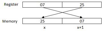
x: memory address
When the processor gets the numeric data from memory to register, it again reverses the bytes. There are two kinds of memory addresses −
- Absolute address - a direct reference of specific location.
- Segment address (or offset) - starting address of a memory segment with the offset value.
Assembly - Environment Setup
Local Environment Setup
Assembly language is dependent upon the instruction set and the architecture of the processor. In this tutorial, we focus on Intel-32 processors like Pentium. To follow this tutorial, you will need −
- An IBM PC or any equivalent compatible computer
- A copy of Linux operating system
- A copy of NASM assembler program
There are many good assembler programs, such as −
- Microsoft Assembler (MASM)
- Borland Turbo Assembler (TASM)
- The GNU assembler (GAS)
We will use the NASM assembler, as it is −
- Free. You can download it from various web sources.
- Well documented and you will get lots of information on net.
- Could be used on both Linux and Windows.
Installing NASM
If you select "Development Tools" while installing Linux, you may get NASM installed along with the Linux operating system and you do not need to download and install it separately. For checking whether you already have NASM installed, take the following steps −
- Open a Linux terminal.
- Type whereis nasm and press ENTER.
- If it is already installed, then a line like, nasm: /usr/bin/nasm appears. Otherwise, you will see just nasm:, then you need to install NASM.
To install NASM, take the following steps −
- Check The netwide assembler (NASM) website for the latest version.
- Download the Linux source archive
nasm-X.XX.ta.gz, whereX.XXis the NASM version number in the archive. - Unpack the archive into a directory which creates a subdirectory
nasm-X. XX. - cd to
nasm-X.XXand type ./configure. This shell script will find the best C compiler to use and set up Makefiles accordingly. - Type make to build the nasm and ndisasm binaries.
- Type make install to install nasm and ndisasm in /usr/local/bin and to install the man pages.
This should install NASM on your system. Alternatively, you can use an RPM distribution for the Fedora Linux. This version is simpler to install, just double-click the RPM file.
Assembly - Basic Syntax
An assembly program can be divided into three sections −
- The data section,
- The bss section, and
- The text section.
The data Section
The data section is used for declaring initialized data or constants. This data does not change at runtime. You can declare various constant values, file names, or buffer size, etc., in this section.
The syntax for declaring data section is −
section.data
The bss Section
The bss section is used for declaring variables. The syntax for declaring bss section is −
section.bss
The text section
The text section is used for keeping the actual code. This section must begin with the declaration global _start, which tells the kernel where the program execution begins.
The syntax for declaring text section is −
section.text
   global _start
_start:
Comments
Assembly language comment begins with a semicolon (;). It may contain any printable character including blank. It can appear on a line by itself, like −
; This program displays a message on screen
or, on the same line along with an instruction, like −
add eax, ebx ; adds ebx to eax
Assembly Language Statements
Assembly language programs consist of three types of statements −
- Executable instructions or instructions,
- Assembler directives or pseudo-ops, and
- Macros.
The executable instructions or simply instructions tell the processor what to do. Each instruction consists of an operation code (opcode). Each executable instruction generates one machine language instruction.
The assembler directives or pseudo-ops tell the assembler about the various aspects of the assembly process. These are non-executable and do not generate machine language instructions.
Macros are basically a text substitution mechanism.
Syntax of Assembly Language Statements
Assembly language statements are entered one statement per line. Each statement follows the following format −
[label] mnemonic [operands] [;comment]
The fields in the square brackets are optional. A basic instruction has two parts, the first one is the name of the instruction (or the mnemonic), which is to be executed, and the second are the operands or the parameters of the command.
Following are some examples of typical assembly language statements −
INC COUNT        ; Increment the memory variable COUNT

MOV TOTAL, 48    ; Transfer the value 48 in the
                 ; memory variable TOTAL

ADD AH, BH       ; Add the content of the
                 ; BH register into the AH register

AND MASK1, 128   ; Perform AND operation on the
                 ; variable MASK1 and 128

ADD MARKS, 10    ; Add 10 to the variable MARKS
MOV AL, 10       ; Transfer the value 10 to the AL register
The Hello World Program in Assembly
The following assembly language code displays the string 'Hello World' on the screen −section .text
   global _start     ;must be declared for linker (ld)

_start:             ;tells linker entry point
   mov edx,len     ;message length
   mov ecx,msg     ;message to write
   mov ebx,1       ;file descriptor (stdout)
   mov eax,4       ;system call number (sys_write)
   int 0x80        ;call kernel

   mov eax,1       ;system call number (sys_exit)
   int 0x80        ;call kernel

section .data
msg db 'Hello, world!', 0xa  ;string to be printed
len equ $ - msg     ;length of the string
When the above code is compiled and executed, it produces the following result −
Hello, world!
Compiling and Linking an Assembly Program in NASM
Make sure you have set the path of nasm and ld binaries in your PATH environment variable. Now, take the following steps for compiling and linking the above program −
- Type the above code using a text editor and save it as hello.asm.
- Make sure that you are in the same directory as where you saved hello.asm.
- To assemble the program, type nasm -f elf hello.asm
- If there is any error, you will be prompted about that at this stage. Otherwise, an object file of your program named hello.o will be created.
- To link the object file and create an executable file named hello, type ld -m elf_i386 -s -o hello hello.o
- Execute the program by typing ./hello
If you have done everything correctly, it will display 'Hello, world!' on the screen.
Assembly - Memory Segments
We have already discussed the three sections of an assembly program. These sections represent various memory segments as well.
Interestingly, if you replace the section keyword with segment, you will get the same result. Try the following code −
segment .text    ;code segment
   global_start    ;must be declared for linker

_start:            ;tell linker entry point
   mov edx,len    ;message length
   mov ecx,msg     ;message to write
   mov ebx,1    ;file descriptor (stdout)
   mov eax,4    ;system call number (sys_write)
   int 0x80    ;call kernel

   mov eax,1       ;system call number (sys_exit)
   int 0x80    ;call kernel

segment .data      ;data segment
msg db 'Hello, world!',0xa   ;our dear string
len equ $ - msg          ;length of our dear string
When the above code is compiled and executed, it produces the following result −
Hello, world!
Memory Segments
A segmented memory model divides the system memory into groups of independent segments referenced by pointers located in the segment registers. Each segment is used to contain a specific type of data. One segment is used to contain instruction codes, another segment stores the data elements, and a third segment keeps the program stack.
In the light of the above discussion, we can specify various memory segments as −
- Data segment − It is represented by .data section and the .bss. The .data section is used to declare the memory region, where data elements are stored for the program. This section cannot be expanded after the data elements are declared, and it remains static throughout the program.The .bss section is also a static memory section that contains buffers for data to be declared later in the program. This buffer memory is zero-filled.
- Code segment − It is represented by .text section. This defines an area in memory that stores the instruction codes. This is also a fixed area.
- Stack − This segment contains data values passed to functions and procedures within the program.
Assembly - Registers
Processor operations mostly involve processing data. This data can be stored in memory and accessed from thereon. However, reading data from and storing data into memory slows down the processor, as it involves complicated processes of sending the data request across the control bus and into the memory storage unit and getting the data through the same channel.
To speed up the processor operations, the processor includes some internal memory storage locations, called registers.
The registers store data elements for processing without having to access the memory. A limited number of registers are built into the processor chip.
Processor Registers
There are ten 32-bit and six 16-bit processor registers in IA-32 architecture. The registers are grouped into three categories −
- General registers,
- Control registers, and
- Segment registers.
The general registers are further divided into the following groups −
- Data registers,
- Pointer registers, and
- Index registers.
Data Registers
Four 32-bit data registers are used for arithmetic, logical, and other operations. These 32-bit registers can be used in three ways −
- As complete 32-bit data registers: EAX, EBX, ECX, EDX.
- Lower halves of the 32-bit registers can be used as four 16-bit data registers: AX, BX, CX and DX.
- Lower and higher halves of the above-mentioned four 16-bit registers can be used as eight 8-bit data registers: AH, AL, BH, BL, CH, CL, DH, and DL.
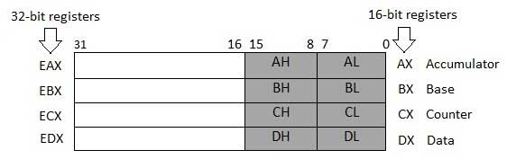
Some of these data registers have specific use in arithmetical operations.
AX is the primary accumulator; it is used in input/output and most arithmetic instructions. For example, in multiplication operation, one operand is stored in EAX or AX or AL register according to the size of the operand.
BX is known as the base register, as it could be used in indexed addressing.
CX is known as the count register, as the ECX, CX registers store the loop count in iterative operations.
DX is known as the data register. It is also used in input/output operations. It is also used with AX register along with DX for multiply and divide operations involving large values.
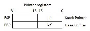
Pointer Registers
The pointer registers are 32-bit EIP, ESP, and EBP registers and corresponding 16-bit right portions IP, SP, and BP. There are three categories of pointer registers −
- Instruction Pointer (IP) − The 16-bit IP register stores the offset address of the next instruction to be executed. IP in association with the CS register (as CS:IP) gives the complete address of the current instruction in the code segment.
- Stack Pointer (SP) − The 16-bit SP register provides the offset value within the program stack. SP in association with the SS register (SS:SP) refers to be current position of data or address within the program stack.
- Base Pointer (BP) − The 16-bit BP register mainly helps in referencing the parameter variables passed to a subroutine. The address in SS register is combined with the offset in BP to get the location of the parameter. BP can also be combined with DI and SI as base register for special addressing.
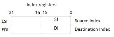
Index Registers
The 32-bit index registers, ESI and EDI, and their 16-bit rightmost portions. SI and DI, are used for indexed addressing and sometimes used in addition and subtraction. There are two sets of index pointers −
- Source Index (SI) − It is used as source index for string operations.
- Destination Index (DI) − It is used as destination index for string operations.
Control Registers
The 32-bit instruction pointer register and the 32-bit flags register combined are considered as the control registers.
Many instructions involve comparisons and mathematical calculations and change the status of the flags and some other conditional instructions test the value of these status flags to take the control flow to other location.
The common flag bits are:
- Overflow Flag (OF) − It indicates the overflow of a high-order bit (leftmost bit) of data after a signed arithmetic operation.
- Direction Flag (DF) − It determines left or right direction for moving or comparing string data. When the DF value is 0, the string operation takes left-to-right direction and when the value is set to 1, the string operation takes right-to-left direction.
- Interrupt Flag (IF) − It determines whether the external interrupts like keyboard entry, etc., are to be ignored or processed. It disables the external interrupt when the value is 0 and enables interrupts when set to 1.
- Trap Flag (TF) − It allows setting the operation of the processor in single-step mode. The DEBUG program we used sets the trap flag, so we could step through the execution one instruction at a time.
- Sign Flag (SF) − It shows the sign of the result of an arithmetic operation. This flag is set according to the sign of a data item following the arithmetic operation. The sign is indicated by the high-order of leftmost bit. A positive result clears the value of SF to 0 and negative result sets it to 1.
- Zero Flag (ZF) − It indicates the result of an arithmetic or comparison operation. A nonzero result clears the zero flag to 0, and a zero result sets it to 1.
- Auxiliary Carry Flag (AF) − It contains the carry from bit 3 to bit 4 following an arithmetic operation; used for specialized arithmetic. The AF is set when a 1-byte arithmetic operation causes a carry from bit 3 into bit 4.
- Parity Flag (PF) − It indicates the total number of 1-bits in the result obtained from an arithmetic operation. An even number of 1-bits clears the parity flag to 0 and an odd number of 1-bits sets the parity flag to 1.
- Carry Flag (CF) − It contains the carry of 0 or 1 from a high-order bit (leftmost) after an arithmetic operation. It also stores the contents of last bit of a shift or rotate operation.
The following table indicates the position of flag bits in the 16-bit Flags register:
| Flag: | O | D | I | T | S | Z | A | P | C | |||||||
|---|---|---|---|---|---|---|---|---|---|---|---|---|---|---|---|---|
| Bit no: | 15 | 14 | 13 | 12 | 11 | 10 | 9 | 8 | 7 | 6 | 5 | 4 | 3 | 2 | 1 | 0 |
Segment Registers
Segments are specific areas defined in a program for containing data, code and stack. There are three main segments −
- Code Segment − It contains all the instructions to be executed. A 16-bit Code Segment register or CS register stores the starting address of the code segment.
- Data Segment − It contains data, constants and work areas. A 16-bit Data Segment register or DS register stores the starting address of the data segment.
- Stack Segment − It contains data and return addresses of procedures or subroutines. It is implemented as a 'stack' data structure. The Stack Segment register or SS register stores the starting address of the stack.
Apart from the DS, CS and SS registers, there are other extra segment registers - ES (extra segment), FS and GS, which provide additional segments for storing data.
In assembly programming, a program needs to access the memory locations. All memory locations within a segment are relative to the starting address of the segment. A segment begins in an address evenly divisible by 16 or hexadecimal 10. So, the rightmost hex digit in all such memory addresses is 0, which is not generally stored in the segment registers.
The segment registers stores the starting addresses of a segment. To get the exact location of data or instruction within a segment, an offset value (or displacement) is required. To reference any memory location in a segment, the processor combines the segment address in the segment register with the offset value of the location.
Example
Look at the following simple program to understand the use of registers in assembly programming. This program displays 9 stars on the screen along with a simple message −
section .text
   global _start  ;must be declared for linker (gcc)

_start:          ;tell linker entry point
   mov edx,len  ;message length
   mov ecx,msg  ;message to write
   mov ebx,1    ;file descriptor (stdout)
   mov eax,4    ;system call number (sys_write)
   int 0x80     ;call kernel

   mov edx,9    ;message length
   mov ecx,s2   ;message to write
   mov ebx,1    ;file descriptor (stdout)
   mov eax,4    ;system call number (sys_write)
   int 0x80     ;call kernel

   mov eax,1    ;system call number (sys_exit)
   int 0x80     ;call kernel

section .data
msg db 'Displaying 9 stars',0xa ;a message
len equ $ - msg  ;length of message
s2 times 9 db '*'
When the above code is compiled and executed, it produces the following result −
Displaying 9 stars
*********
Assembly - System Calls
System calls are APIs for the interface between the user space and the kernel space. We have already used the system calls. sys_write and sys_exit, for writing into the screen and exiting from the program, respectively.
Linux System Calls
You can make use of Linux system calls in your assembly programs. You need to take the following steps for using Linux system calls in your program −
- Put the system call number in the EAX register.
- Store the arguments to the system call in the registers EBX, ECX, etc.
- Call the relevant interrupt (80h).
- The result is usually returned in the EAX register.
There are six registers that store the arguments of the system call used. These are the EBX, ECX, EDX, ESI, EDI, and EBP. These registers take the consecutive arguments, starting with the EBX register. If there are more than six arguments, then the memory location of the first argument is stored in the EBX register.
The following code snippet shows the use of the system call sys_exit −
mov eax,1  ; system call number (sys_exit)
int 0x80  ; call kernel
The following code snippet shows the use of the system call sys_write −
mov edx,4  ; message length
mov ecx,msg  ; message to write
mov ebx,1  ; file descriptor (stdout)
mov eax,4  ; system call number (sys_write)
int 0x80  ; call kernel
All the syscalls are listed in /usr/include/asm/unistd.h, together with their numbers (the value to put in EAX before you call int 80h).
The following table shows some of the system calls used in this tutorial −
| %eax | Name | %ebx | %ecx | %edx | %esx | %edi |
|---|---|---|---|---|---|---|
| 1 | sys_exit | int | - | - | - | - |
| 2 | sys_fork | struct pt_regs | - | - | - | - |
| 3 | sys_read | unsigned int | char * | size_t | - | - |
| 4 | sys_write | unsigned int | const char * | size_t | - | - |
| 5 | sys_open | const char * | int | int | - | - |
| 6 | sys_close | unsigned int | - | - | - | - |
Example
The following example reads a number from the keyboard and displays it on the screen −
section .data                           ;Data segment
   userMsg db 'Please enter a number: ' ;Ask the user to enter a number
   lenUserMsg equ $-userMsg             ;The length of the message
   dispMsg db 'You have entered: '
   lenDispMsg equ $-dispMsg

section .bss           ;Uninitialized data
   num resb 5

section .text          ;Code Segment
   global _start

_start:                ;User prompt
   mov eax, 4
   mov ebx, 1
   mov ecx, userMsg
   mov edx, lenUserMsg
   int 80h

   ;Read and store the user input
   mov eax, 3
   mov ebx, 2
   mov ecx, num
   mov edx, 5          ;5 bytes (numeric, 1 for sign) of that information
   int 80h

   ;Output the message 'The entered number is: '
   mov eax, 4
   mov ebx, 1
   mov ecx, dispMsg
   mov edx, lenDispMsg
   int 80h

   ;Output the number entered
   mov eax, 4
   mov ebx, 1
   mov ecx, num
   mov edx, 5
   int 80h

   ; Exit code
   mov eax, 1
   mov ebx, 0
   int 80h
When the above code is compiled and executed, it produces the following result −
Please enter a number:
1234
You have entered:1234
Assembly - Addressing Modes
Most assembly language instructions require operands to be processed. An operand address provides the location, where the data to be processed is stored. Some instructions do not require an operand, whereas some other instructions may require one, two, or three operands.
When an instruction requires two operands, the first operand is generally the destination, which contains data in a register or memory location and the second operand is the source. Source contains either the data to be delivered (immediate addressing) or the address (in register or memory) of the data. Generally, the source data remains unaltered after the operation.
The three basic modes of addressing are −
- Register addressing
- Immediate addressing
- Memory addressing
Register Addressing
In this addressing mode, a register contains the operand. Depending upon the instruction, the register may be the first operand, the second operand or both.
For example,
MOV DX, TAX_RATE   ; Register in first operand
MOV COUNT, CX    ; Register in second operand
MOV EAX, EBX    ; Both the operands are in registers
As processing data between registers does not involve memory, it provides fastest processing of data.
Immediate Addressing
An immediate operand has a constant value or an expression. When an instruction with two operands uses immediate addressing, the first operand may be a register or memory location, and the second operand is an immediate constant. The first operand defines the length of the data.
For example,
BYTE_VALUE  DB  150    ; A byte value is defined
WORD_VALUE  DW  300    ; A word value is defined
ADD  BYTE_VALUE, 65    ; An immediate operand 65 is added
MOV  AX, 45H           ; Immediate constant 45H is transferred to AX
Direct Memory Addressing
When operands are specified in memory addressing mode, direct access to main memory, usually to the data segment, is required. This way of addressing results in slower processing of data. To locate the exact location of data in memory, we need the segment start address, which is typically found in the DS register and an offset value. This offset value is also called effective address.
In direct addressing mode, the offset value is specified directly as part of the instruction, usually indicated by the variable name. The assembler calculates the offset value and maintains a symbol table, which stores the offset values of all the variables used in the program.
In direct memory addressing, one of the operands refers to a memory location and the other operand references a register.
For example,
ADD BYTE_VALUE, DL ; Adds the register in the memory location
MOV BX, WORD_VALUE ; Operand from the memory is added to register
Direct-Offset Addressing
This addressing mode uses the arithmetic operators to modify an address. For example, look at the following definitions that define tables of data −
BYTE_TABLE DB  14, 15, 22, 45      ; Tables of bytes
WORD_TABLE DW  134, 345, 564, 123  ; Tables of words
The following operations access data from the tables in the memory into registers −
MOV CL, BYTE_TABLE[2] ; Gets the 3rd element of the BYTE_TABLE
MOV CL, BYTE_TABLE + 2 ; Gets the 3rd element of the BYTE_TABLE
MOV CX, WORD_TABLE[3] ; Gets the 4th element of the WORD_TABLE
MOV CX, WORD_TABLE + 3 ; Gets the 4th element of the WORD_TABLE
Indirect Memory Addressing
This addressing mode utilizes the computer's ability of Segment:Offset addressing. Generally, the base registers EBX, EBP (or BX, BP) and the index registers (DI, SI), coded within square brackets for memory references, are used for this purpose.
Indirect addressing is generally used for variables containing several elements like, arrays. Starting address of the array is stored in, say, the EBX register.
The following code snippet shows how to access different elements of the variable.
MY_TABLE TIMES 10 DW 0  ; Allocates 10 words (2 bytes) each initialized to 0
MOV EBX, [MY_TABLE]     ; Effective Address of MY_TABLE in EBX
MOV [EBX], 110          ; MY_TABLE[0] = 110
ADD EBX, 2              ; EBX = EBX +2
MOV [EBX], 123          ; MY_TABLE[1] = 123
The MOV Instruction
We have already used the MOV instruction that is used for moving data from one storage space to another. The MOV instruction takes two operands.
Syntax
The syntax of the MOV instruction is −
MOV destination, source
The MOV instruction may have one of the following five forms −
MOV  register, register
MOV  register, immediate
MOV  memory, immediate
MOV  register, memory
MOV  memory, register
Please note that −
- Both the operands in MOV operation should be of same size
- The value of source operand remains unchanged
The MOV instruction causes ambiguity at times. For example, look at the statements −
MOV  EBX, [MY_TABLE]  ; Effective Address of MY_TABLE in EBX
MOV  [EBX], 110       ; MY_TABLE[0] = 110
It is not clear whether you want to move a byte equivalent or word equivalent of the number 110. In such cases, it is wise to use a type specifier.
Following table shows some of the common type specifiers −
| Type Specifier | Bytes addressed |
|---|---|
| BYTE | 1 |
| WORD | 2 |
| DWORD | 4 |
| QWORD | 8 |
| TBYTE | 10 |
Example
The following program illustrates some of the concepts discussed above. It stores a name 'Zara Ali' in the data section of the memory, then changes its value to another name 'Nuha Ali' programmatically and displays both the names.
section .text
   global_start     ;must be declared for linker (ld)
_start:             ;tell linker entry point

   ;writing the name 'Zara Ali'
   mov edx,9       ;message length
   mov ecx, name   ;message to write
   mov ebx,1       ;file descriptor (stdout)
   mov eax,4       ;system call number (sys_write)
   int 0x80        ;call kernel

   mov [name],  dword 'Nuha'    ; Changed the name to Nuha Ali

   ;writing the name 'Nuha Ali'
   mov edx,8       ;message length
   mov ecx,name    ;message to write
   mov ebx,1       ;file descriptor (stdout)
   mov eax,4       ;system call number (sys_write)
   int 0x80        ;call kernel

   mov eax,1       ;system call number (sys_exit)
   int 0x80        ;call kernel

section .data
name db 'Zara Ali '
When the above code is compiled and executed, it produces the following result −
Zara Ali Nuha Ali
Assembly - Variables
NASM provides various define directives for reserving storage space for variables. The define assembler directive is used for allocation of storage space. It can be used to reserve as well as initialize one or more bytes.
Allocating Storage Space for Initialized Data
The syntax for storage allocation statement for initialized data is −
[variable-name] define-directive initial-value [,initial-value]...
Where, variable-name is the identifier for each storage space. The assembler associates an offset value for each variable name defined in the data segment.
There are five basic forms of the define directive −
| Directive | Purpose | Storage Space |
|---|---|---|
| DB | Define Byte | allocates 1 byte |
| DW | Define Word | allocates 2 bytes |
| DD | Define Doubleword | allocates 4 bytes |
| DQ | Define Quadword | allocates 8 bytes |
| DT | Define Ten Bytes | allocates 10 bytes |
Following are some examples of using define directives −
choice  DB 'y'
number  DW 12345
neg_number DW -12345
big_number DQ 123456789
real_number1 DD 1.234
real_number2 DQ 123.456
Please note that −
- Each byte of character is stored as its ASCII value in hexadecimal.
- Each decimal value is automatically converted to its 16-bit binary equivalent and stored as a hexadecimal number.
- Processor uses the little-endian byte ordering.
- Negative numbers are converted to its 2's complement representation.
- Short and long floating-point numbers are represented using 32 or 64 bits, respectively.
The following program shows the use of define directive −
Assembly - Logical Instructions
The processor instruction set provides the instructions AND, OR, XOR, TEST, and NOT Boolean logic, which tests, sets, and clears the bits according to the need of the program.
The format for these instructions −
| Sr.No. | Instruction | Format |
|---|---|---|
| 1 | AND | AND operand1, operand2 |
| 2 | OR | OR operand1, operand2 |
| 3 | XOR | XOR operand1, operand2 |
| 4 | TEST | TEST operand1, operand2 |
| 5 | NOT | NOT operand1 |
The first operand in all the cases could be either in register or in memory. The second operand could be either in register/memory or an immediate (constant) value. However, memory-to-memory operations are not possible. These instructions compare or match bits of the operands and set the CF, OF, PF, SF and ZF flags.
The AND Instruction
The AND instruction is used for supporting logical expressions by performing bitwise AND operation. The bitwise AND operation returns 1, if the matching bits from both the operands are 1, otherwise it returns 0. For example −
             Operand1:  0101
             Operand2:  0011
----------------------------
After AND -> Operand1: 0001
The AND operation can be used for clearing one or more bits. For example, say the BL register contains 0011 1010. If you need to clear the high-order bits to zero, you AND it with 0FH.
AND BL, 0FH ; This sets BL to 0000 1010
Let's take up another example. If you want to check whether a given number is odd or even, a simple test would be to check the least significant bit of the number. If this is 1, the number is odd, else the number is even.
Assuming the number is in AL register, we can write −
AND AL, 01H     ; ANDing with 0000 0001
JZ    EVEN_NUMBER
Example
section .text
   global _start            ;must be declared for using gcc

_start:                     ;tell linker entry point
   mov   ax,   8h           ;getting 8 in the ax
   and   ax, 1              ;and ax with 1
   jz    evnn
   mov   eax, 4             ;system call number (sys_write)
   mov   ebx, 1             ;file descriptor (stdout)
   mov   ecx, odd_msg       ;message to write
   mov   edx, len2          ;length of message
   int   0x80               ;call kernel
   jmp   outprog

evnn:

   mov   ah,  09h
   mov   eax, 4             ;system call number (sys_write)
   mov   ebx, 1             ;file descriptor (stdout)
   mov   ecx, even_msg      ;message to write
   mov   edx, len1          ;length of message
   int   0x80               ;call kernel

outprog:

   mov   eax,1              ;system call number (sys_exit)
   int   0x80               ;call kernel

section   .data
even_msg  db  'Even Number!' ;message showing even number
len1  equ  $ - even_msg

odd_msg db  'Odd Number!'    ;message showing odd number
len2  equ  $ - odd_msg
When the above code is compiled and executed, it produces the following result −
Even Number!
Change the value in the ax register with an odd digit, like −
mov ax, 9h ; getting 9 in the ax
The program would display:
Odd Number!
Similarly to clear the entire register you can AND it with 00H.
The OR Instruction
The OR instruction is used for supporting logical expression by performing bitwise OR operation. The bitwise OR operator returns 1, if the matching bits from either or both operands are one. It returns 0, if both the bits are zero.
For example,
             Operand1:     0101
             Operand2:     0011
----------------------------
After OR -> Operand1:    0111
The OR operation can be used for setting one or more bits. For example, let us assume the AL register contains 0011 1010, you need to set the four low-order bits, you can OR it with a value 0000 1111, i.e., FH.
OR BL, 0FH ; This sets BL to 0011 1111
Example
The following example demonstrates the OR instruction. Let us store the value 5 and 3 in the AL and the BL registers, respectively, then the instruction,
OR AL, BL
should store 7 in the AL register −
Live Demosection .text
global _start ;must be declared for using gcc
_start: ;tell linker entry point
mov al, 5 ;getting 5 in the al
mov bl, 3 ;getting 3 in the bl
or al, bl ;or al and bl registers, result should be 7
add al, byte '0' ;converting decimal to ascii
mov [result], al
mov eax, 4
mov ebx, 1
mov ecx, result
mov edx, 1
int 0x80
outprog:
mov eax,1 ;system call number (sys_exit)
int 0x80 ;call kernel
section .bss
result resb 1
When the above code is compiled and executed, it produces the following result −
7
The XOR Instruction
The XOR instruction implements the bitwise XOR operation. The XOR operation sets the resultant bit to 1, if and only if the bits from the operands are different. If the bits from the operands are same (both 0 or both 1), the resultant bit is cleared to 0.
For example,
             Operand1:     0101
             Operand2:     0011
----------------------------
After XOR -> Operand1:    0110
XORing an operand with itself changes the operand to 0. This is used to clear a register.
XOR EAX, EAX
The TEST Instruction
The TEST instruction works same as the AND operation, but unlike AND instruction, it does not change the first operand. So, if we need to check whether a number in a register is even or odd, we can also do this using the TEST instruction without changing the original number.
TEST    AL, 01H
JZ      EVEN_NUMBER
The NOT Instruction
The NOT instruction implements the bitwise NOT operation. NOT operation reverses the bits in an operand. The operand could be either in a register or in the memory.
For example,
             Operand1:    0101 0011
After NOT -> Operand1:    1010 1100
Assembly - Conditions
Conditional execution in assembly language is accomplished by several looping and branching instructions. These instructions can change the flow of control in a program. Conditional execution is observed in two scenarios −
| Sr.No. | Conditional Instructions |
|---|---|
| 1 |
Unconditional jump
This is performed by the JMP instruction. Conditional execution often involves a transfer of control to the address of an instruction that does not follow the currently executing instruction. Transfer of control may be forward, to execute a new set of instructions or backward, to re-execute the same steps.
|
| 2 |
Conditional jump
This is performed by a set of jump instructions j<condition> depending upon the condition. The conditional instructions transfer the control by breaking the sequential flow and they do it by changing the offset value in IP.
|
Let us discuss the CMP instruction before discussing the conditional instructions.
CMP Instruction
The CMP instruction compares two operands. It is generally used in conditional execution. This instruction basically subtracts one operand from the other for comparing whether the operands are equal or not. It does not disturb the destination or source operands. It is used along with the conditional jump instruction for decision making.
Syntax
CMP destination, source
CMP compares two numeric data fields. The destination operand could be either in register or in memory. The source operand could be a constant (immediate) data, register or memory.
Example
CMP DX, 00  ; Compare the DX value with zero
JE  L7      ; If yes, then jump to label L7
.
.
L7: ...
CMP is often used for comparing whether a counter value has reached the number of times a loop needs to be run. Consider the following typical condition −
INC EDX
CMP EDX, 10 ; Compares whether the counter has reached 10
JLE LP1     ; If it is less than or equal to 10, then jump to LP1
Unconditional Jump
As mentioned earlier, this is performed by the JMP instruction. Conditional execution often involves a transfer of control to the address of an instruction that does not follow the currently executing instruction. Transfer of control may be forward, to execute a new set of instructions or backward, to re-execute the same steps.
Syntax
The JMP instruction provides a label name where the flow of control is transferred immediately. The syntax of the JMP instruction is −
JMP label
Example
The following code snippet illustrates the JMP instruction −
MOV  AX, 00    ; Initializing AX to 0
MOV  BX, 00    ; Initializing BX to 0
MOV  CX, 01    ; Initializing CX to 1
L20:
ADD  AX, 01    ; Increment AX
ADD  BX, AX    ; Add AX to BX
SHL  CX, 1     ; shift left CX, this in turn doubles the CX value
JMP  L20       ; repeats the statements
Conditional Jump
If some specified condition is satisfied in conditional jump, the control flow is transferred to a target instruction. There are numerous conditional jump instructions depending upon the condition and data.
Following are the conditional jump instructions used on signed data used for arithmetic operations −
| Instruction | Description | Flags tested |
|---|---|---|
| JE/JZ | Jump Equal or Jump Zero | ZF |
| JNE/JNZ | Jump not Equal or Jump Not Zero | ZF |
| JG/JNLE | Jump Greater or Jump Not Less/Equal | OF, SF, ZF |
| JGE/JNL | Jump Greater/Equal or Jump Not Less | OF, SF |
| JL/JNGE | Jump Less or Jump Not Greater/Equal | OF, SF |
| JLE/JNG | Jump Less/Equal or Jump Not Greater | OF, SF, ZF |
Following are the conditional jump instructions used on unsigned data used for logical operations −
| Instruction | Description | Flags tested |
|---|---|---|
| JE/JZ | Jump Equal or Jump Zero | ZF |
| JNE/JNZ | Jump not Equal or Jump Not Zero | ZF |
| JA/JNBE | Jump Above or Jump Not Below/Equal | CF, ZF |
| JAE/JNB | Jump Above/Equal or Jump Not Below | CF |
| JB/JNAE | Jump Below or Jump Not Above/Equal | CF |
| JBE/JNA | Jump Below/Equal or Jump Not Above | AF, CF |
The following conditional jump instructions have special uses and check the value of flags −
| Instruction | Description | Flags tested |
|---|---|---|
| JXCZ | Jump if CX is Zero | none |
| JC | Jump If Carry | CF |
| JNC | Jump If No Carry | CF |
| JO | Jump If Overflow | OF |
| JNO | Jump If No Overflow | OF |
| JP/JPE | Jump Parity or Jump Parity Even | PF |
| JNP/JPO | Jump No Parity or Jump Parity Odd | PF |
| JS | Jump Sign (negative value) | SF |
| JNS | Jump No Sign (positive value) | SF |
The syntax for the J<condition> set of instructions −
Example,
CMP AL, BL
JE EQUAL
CMP AL, BH
JE EQUAL
CMP AL, CL
JE EQUAL
NON_EQUAL: ...
EQUAL: ...
Example
The following program displays the largest of three variables. The variables are double-digit variables. The three variables num1, num2 and num3 have values 47, 22 and 31, respectively −
section .text
   global _start         ;must be declared for using gcc

_start:                  ;tell linker entry point
   mov   ecx, [num1]
   cmp   ecx, [num2]
   jg    check_third_num
   mov   ecx, [num2]

 check_third_num:

   cmp   ecx, [num3]
   jg    _exit
   mov   ecx, [num3]

 _exit:

   mov   [largest], ecx
   mov   ecx,msg
   mov   edx, len
   mov   ebx,1 ;file descriptor (stdout)
   mov   eax,4 ;system call number (sys_write)
   int   0x80 ;call kernel

   mov   ecx,largest
   mov   edx, 2
   mov   ebx,1 ;file descriptor (stdout)
   mov   eax,4 ;system call number (sys_write)
   int   0x80 ;call kernel

   mov   eax, 1
   int   80h

section .data

   msg db "The largest digit is: ", 0xA,0xD
   len equ $- msg
   num1 dd '47'
   num2 dd '22'
   num3 dd '31'

segment .bss
   largest resb 2
When the above code is compiled and executed, it produces the following result −
The largest digit is:
47
Assembly - Loops
The JMP instruction can be used for implementing loops. For example, the following code snippet can be used for executing the loop-body 10 times.
MOV CL, 10
L1:
<LOOP-BODY>
DEC CL
JNZ L1
The processor instruction set, however, includes a group of loop instructions for implementing iteration. The basic LOOP instruction has the following syntax −
LOOP label
Where, label is the target label that identifies the target instruction as in the jump instructions. The LOOP instruction assumes that the ECX register contains the loop count. When the loop instruction is executed, the ECX register is decremented and the control jumps to the target label, until the ECX register value, i.e., the counter reaches the value zero.
The above code snippet could be written as −
mov ECX,10
l1:
<loop body>
loop l1
Example
The following program prints the number 1 to 9 on the screen
section .text
   global _start        ;must be declared for using gcc

_start:                 ;tell linker entry point
   mov ecx,10
   mov eax, '1'

l1:
   mov [num], eax
   mov eax, 4
   mov ebx, 1
   push ecx

   mov ecx, num
   mov edx, 1
   int 0x80

   mov eax, [num]
   sub eax, '0'
   inc eax
   add eax, '0'
   pop ecx
   loop l1

   mov eax,1             ;system call number (sys_exit)
   int 0x80              ;call kernel
section .bss
num resb 1
When the above code is compiled and executed, it produces the following result −
123456789:
Assembly - Numbers
Numerical data is generally represented in binary system. Arithmetic instructions operate on binary data. When numbers are displayed on screen or entered from keyboard, they are in ASCII form.
So far, we have converted this input data in ASCII form to binary for arithmetic calculations and converted the result back to binary. The following code shows this −
section .text
   global _start        ;must be declared for using gcc

_start:                 ;tell linker entry point
   mov eax,'3'
   sub     eax, '0'

   mov  ebx, '4'
   sub     ebx, '0'
   add  eax, ebx
   add eax, '0'

   mov  [sum], eax
   mov ecx,msg
   mov edx, len
   mov ebx,1          ;file descriptor (stdout)
   mov eax,4          ;system call number (sys_write)
   int 0x80          ;call kernel

   mov ecx,sum
   mov edx, 1
   mov ebx,1          ;file descriptor (stdout)
   mov eax,4          ;system call number (sys_write)
   int 0x80          ;call kernel

   mov eax,1          ;system call number (sys_exit)
   int 0x80          ;call kernel

section .data
msg db "The sum is:", 0xA,0xD
len equ $ - msg
segment .bss
sum resb 1
When the above code is compiled and executed, it produces the following result −
The sum is:
7
Such conversions, however, have an overhead, and assembly language programming allows processing numbers in a more efficient way, in the binary form. Decimal numbers can be represented in two forms −
- ASCII form
- BCD or Binary Coded Decimal form
ASCII Representation
In ASCII representation, decimal numbers are stored as string of ASCII characters. For example, the decimal value 1234 is stored as −
31 32 33 34H
Where, 31H is ASCII value for 1, 32H is ASCII value for 2, and so on. There are four instructions for processing numbers in ASCII representation −
- AAA − ASCII Adjust After Addition
- AAS − ASCII Adjust After Subtraction
- AAM − ASCII Adjust After Multiplication
- AAD − ASCII Adjust Before Division
These instructions do not take any operands and assume the required operand to be in the AL register.
The following example uses the AAS instruction to demonstrate the concept −
section .text
   global _start        ;must be declared for using gcc

_start:                 ;tell linker entry point
   sub     ah, ah
   mov     al, '9'
   sub     al, '3'
   aas
   or      al, 30h
   mov     [res], ax

   mov edx,len         ;message length
   mov ecx,msg         ;message to write
   mov ebx,1         ;file descriptor (stdout)
   mov eax,4         ;system call number (sys_write)
   int 0x80         ;call kernel

   mov edx,1         ;message length
   mov ecx,res         ;message to write
   mov ebx,1         ;file descriptor (stdout)
   mov eax,4         ;system call number (sys_write)
   int 0x80         ;call kernel

   mov eax,1         ;system call number (sys_exit)
   int 0x80         ;call kernel

section .data
msg db 'The Result is:',0xa
len equ $ - msg
section .bss
res resb 1
When the above code is compiled and executed, it produces the following result −
The Result is:
6
BCD Representation
There are two types of BCD representation −
- Unpacked BCD representation
- Packed BCD representation
In unpacked BCD representation, each byte stores the binary equivalent of a decimal digit. For example, the number 1234 is stored as −
01 02 03 04H
There are two instructions for processing these numbers −
- AAM − ASCII Adjust After Multiplication
- AAD − ASCII Adjust Before Division
The four ASCII adjust instructions, AAA, AAS, AAM, and AAD, can also be used with unpacked BCD representation. In packed BCD representation, each digit is stored using four bits. Two decimal digits are packed into a byte. For example, the number 1234 is stored as −
12 34H
There are two instructions for processing these numbers −
- DAA − Decimal Adjust After Addition
- DAS − decimal Adjust After Subtraction
There is no support for multiplication and division in packed BCD representation.
Example
The following program adds up two 5-digit decimal numbers and displays the sum. It uses the above concepts −
section .text
   global _start        ;must be declared for using gcc

_start:                 ;tell linker entry point

   mov     esi, 4       ;pointing to the rightmost digit
   mov     ecx, 5       ;num of digits
   clc
add_loop:
   mov  al, [num1 + esi]
   adc  al, [num2 + esi]
   aaa
   pushf
   or  al, 30h
   popf

   mov [sum + esi], al
   dec esi
   loop add_loop

   mov edx,len         ;message length
   mov ecx,msg         ;message to write
   mov ebx,1         ;file descriptor (stdout)
   mov eax,4         ;system call number (sys_write)
   int 0x80         ;call kernel

   mov edx,5         ;message length
   mov ecx,sum         ;message to write
   mov ebx,1         ;file descriptor (stdout)
   mov eax,4         ;system call number (sys_write)
   int 0x80         ;call kernel

   mov eax,1         ;system call number (sys_exit)
   int 0x80         ;call kernel

section .data
msg db 'The Sum is:',0xa
len equ $ - msg
num1 db '12345'
num2 db '23456'
sum db '     '
When the above code is compiled and executed, it produces the following result −
The Sum is:
35801
Assembly - Strings
We have already used variable length strings in our previous examples. The variable length strings can have as many characters as required. Generally, we specify the length of the string by either of the two ways −
- Explicitly storing string length
- Using a sentinel character
We can store the string length explicitly by using the $ location counter symbol that represents the current value of the location counter. In the following example −
msg  db  'Hello, world!',0xa ;our dear string
len  equ  $ - msg            ;length of our dear string
$ points to the byte after the last character of the string variable msg. Therefore, $-msg gives the length of the string. We can also write
msg db 'Hello, world!',0xa ;our dear string
len equ 13                 ;length of our dear string
Alternatively, you can store strings with a trailing sentinel character to delimit a string instead of storing the string length explicitly. The sentinel character should be a special character that does not appear within a string.
For example −
message DB 'I am loving it!', 0
String Instructions
Each string instruction may require a source operand, a destination operand or both. For 32-bit segments, string instructions use ESI and EDI registers to point to the source and destination operands, respectively.
For 16-bit segments, however, the SI and the DI registers are used to point to the source and destination, respectively.
There are five basic instructions for processing strings. They are −
- MOVS − This instruction moves 1 Byte, Word or Doubleword of data from memory location to another.
- LODS − This instruction loads from memory. If the operand is of one byte, it is loaded into the AL register, if the operand is one word, it is loaded into the AX register and a doubleword is loaded into the EAX register.
- STOS − This instruction stores data from register (AL, AX, or EAX) to memory.
- CMPS − This instruction compares two data items in memory. Data could be of a byte size, word or doubleword.
- SCAS − This instruction compares the contents of a register (AL, AX or EAX) with the contents of an item in memory.
Each of the above instruction has a byte, word, and doubleword version, and string instructions can be repeated by using a repetition prefix.
These instructions use the ES:DI and DS:SI pair of registers, where DI and SI registers contain valid offset addresses that refers to bytes stored in memory. SI is normally associated with DS (data segment) and DI is always associated with ES (extra segment).
The DS:SI (or ESI) and ES:DI (or EDI) registers point to the source and destination operands, respectively. The source operand is assumed to be at DS:SI (or ESI) and the destination operand at ES:DI (or EDI) in memory.
For 16-bit addresses, the SI and DI registers are used, and for 32-bit addresses, the ESI and EDI registers are used.
The following table provides various versions of string instructions and the assumed space of the operands.
| Basic Instruction | Operands at | Byte Operation | Word Operation | Double word Operation |
|---|---|---|---|---|
| MOVS | ES:DI, DS:SI | MOVSB | MOVSW | MOVSD |
| LODS | AX, DS:SI | LODSB | LODSW | LODSD |
| STOS | ES:DI, AX | STOSB | STOSW | STOSD |
| CMPS | DS:SI, ES: DI | CMPSB | CMPSW | CMPSD |
| SCAS | ES:DI, AX | SCASB | SCASW | SCASD |
Repetition Prefixes
The REP prefix, when set before a string instruction, for example - REP MOVSB, causes repetition of the instruction based on a counter placed at the CX register. REP executes the instruction, decreases CX by 1, and checks whether CX is zero. It repeats the instruction processing until CX is zero.
The Direction Flag (DF) determines the direction of the operation.
- Use CLD (Clear Direction Flag, DF = 0) to make the operation left to right.
- Use STD (Set Direction Flag, DF = 1) to make the operation right to left.
The REP prefix also has the following variations:
- REP: It is the unconditional repeat. It repeats the operation until CX is zero.
- REPE or REPZ: It is conditional repeat. It repeats the operation while the zero flag indicates equal/zero. It stops when the ZF indicates not equal/zero or when CX is zero.
- REPNE or REPNZ: It is also conditional repeat. It repeats the operation while the zero flag indicates not equal/zero. It stops when the ZF indicates equal/zero or when CX is decremented to zero.
Assembly - Arrays
We have already discussed that the data definition directives to the assembler are used for allocating storage for variables. The variable could also be initialized with some specific value. The initialized value could be specified in hexadecimal, decimal or binary form.
For example, we can define a word variable 'months' in either of the following way −
MONTHS DW 12
MONTHS DW 0CH
MONTHS DW 0110B
The data definition directives can also be used for defining a one-dimensional array. Let us define a one-dimensional array of numbers.
NUMBERS DW 34, 45, 56, 67, 75, 89
The above definition declares an array of six words each initialized with the numbers 34, 45, 56, 67, 75, 89. This allocates 2x6 = 12 bytes of consecutive memory space. The symbolic address of the first number will be NUMBERS and that of the second number will be NUMBERS + 2 and so on.
Let us take up another example. You can define an array named inventory of size 8, and initialize all the values with zero, as −
INVENTORY   DW  0
            DW  0
            DW  0
            DW  0
            DW  0
            DW  0
            DW  0
            DW  0
Which can be abbreviated as −
INVENTORY DW 0, 0 , 0 , 0 , 0 , 0 , 0 , 0
The TIMES directive can also be used for multiple initializations to the same value. Using TIMES, the INVENTORY array can be defined as:
INVENTORY TIMES 8 DW 0
Example
The following example demonstrates the above concepts by defining a 3-element array x, which stores three values: 2, 3 and 4. It adds the values in the array and displays the sum 9 −
section .text
   global _start   ;must be declared for linker (ld)

_start:

   mov  eax,3      ;number bytes to be summed
   mov  ebx,0      ;EBX will store the sum
   mov  ecx, x     ;ECX will point to the current element to be summed

top:  add  ebx, [ecx]

   add  ecx,1      ;move pointer to next element
   dec  eax        ;decrement counter
   jnz  top        ;if counter not 0, then loop again

done:

   add   ebx, '0'
   mov  [sum], ebx ;done, store result in "sum"

display:

   mov  edx,1      ;message length
   mov  ecx, sum   ;message to write
   mov  ebx, 1     ;file descriptor (stdout)
   mov  eax, 4     ;system call number (sys_write)
   int  0x80       ;call kernel

   mov  eax, 1     ;system call number (sys_exit)
   int  0x80       ;call kernel

section .data
global x
x:
   db  2
   db  4
   db  3

sum:
   db  0
When the above code is compiled and executed, it produces the following result −
9
Assembly - Procedures
Procedures or subroutines are very important in assembly language, as the assembly language programs tend to be large in size. Procedures are identified by a name. Following this name, the body of the procedure is described which performs a well-defined job. End of the procedure is indicated by a return statement.
Syntax
Following is the syntax to define a procedure −
proc_name:
   procedure body
   ...
   ret
The procedure is called from another function by using the CALL instruction. The CALL instruction should have the name of the called procedure as an argument as shown below −
CALL proc_name
The called procedure returns the control to the calling procedure by using the RET instruction.
Example
Let us write a very simple procedure named sum that adds the variables stored in the ECX and EDX register and returns the sum in the EAX register −
section .text
   global _start        ;must be declared for using gcc

_start:                 ;tell linker entry point
   mov ecx,'4'
   sub     ecx, '0'

   mov  edx, '5'
   sub     edx, '0'

   call    sum          ;call sum procedure
   mov  [res], eax
   mov ecx, msg
   mov edx, len
   mov ebx,1         ;file descriptor (stdout)
   mov eax,4         ;system call number (sys_write)
   int 0x80         ;call kernel

   mov ecx, res
   mov edx, 1
   mov ebx, 1         ;file descriptor (stdout)
   mov eax, 4         ;system call number (sys_write)
   int 0x80         ;call kernel

   mov eax,1         ;system call number (sys_exit)
   int 0x80         ;call kernel
sum:
   mov     eax, ecx
   add     eax, edx
   add     eax, '0'
   ret

section .data
msg db "The sum is:", 0xA,0xD
len equ $- msg

segment .bss
res resb 1
When the above code is compiled and executed, it produces the following result −
The sum is:
9
Stacks Data Structure
A stack is an array-like data structure in the memory in which data can be stored and removed from a location called the 'top' of the stack. The data that needs to be stored is 'pushed' into the stack and data to be retrieved is 'popped' out from the stack. Stack is a LIFO data structure, i.e., the data stored first is retrieved last.
Assembly language provides two instructions for stack operations: PUSH and POP. These instructions have syntaxes like −
PUSH    operand
POP     address/register
The memory space reserved in the stack segment is used for implementing stack. The registers SS and ESP (or SP) are used for implementing the stack. The top of the stack, which points to the last data item inserted into the stack is pointed to by the SS:ESP register, where the SS register points to the beginning of the stack segment and the SP (or ESP) gives the offset into the stack segment.
The stack implementation has the following characteristics −
- Only words or doublewords could be saved into the stack, not a byte.
- The stack grows in the reverse direction, i.e., toward the lower memory address
- The top of the stack points to the last item inserted in the stack; it points to the lower byte of the last word inserted.
As we discussed about storing the values of the registers in the stack before using them for some use; it can be done in following way −
; Save the AX and BX registers in the stack
PUSH    AX
PUSH    BX

; Use the registers for other purpose
MOV AX, VALUE1
MOV  BX, VALUE2
...
MOV  VALUE1, AX
MOV VALUE2, BX

; Restore the original values
POP AX
POP BX
Example
The following program displays the entire ASCII character set. The main program calls a procedure named display, which displays the ASCII character set.
section .text
   global _start        ;must be declared for using gcc

_start:                 ;tell linker entry point
   call    display
   mov eax,1         ;system call number (sys_exit)
   int 0x80         ;call kernel

display:
   mov    ecx, 256

next:
   push    ecx
   mov     eax, 4
   mov     ebx, 1
   mov     ecx, achar
   mov     edx, 1
   int     80h

   pop     ecx
   mov dx, [achar]
   cmp byte [achar], 0dh
   inc byte [achar]
   loop    next
   ret

section .data
achar db '0'
When the above code is compiled and executed, it produces the following result −
0123456789:;<=>?@ABCDEFGHIJKLMNOPQRSTUVWXYZ[\]^_`abcdefghijklmnopqrstuvwxyz{|}
...
...
Assembly - Recursion
A recursive procedure is one that calls itself. There are two kind of recursion: direct and indirect. In direct recursion, the procedure calls itself and in indirect recursion, the first procedure calls a second procedure, which in turn calls the first procedure.
Recursion could be observed in numerous mathematical algorithms. For example, consider the case of calculating the factorial of a number. Factorial of a number is given by the equation −
Fact (n) = n * fact (n-1) for n > 0
For example: factorial of 5 is 1 x 2 x 3 x 4 x 5 = 5 x factorial of 4 and this can be a good example of showing a recursive procedure. Every recursive algorithm must have an ending condition, i.e., the recursive calling of the program should be stopped when a condition is fulfilled. In the case of factorial algorithm, the end condition is reached when n is 0.
The following program shows how factorial n is implemented in assembly language. To keep the program simple, we will calculate factorial 3.
section .text
   global _start         ;must be declared for using gcc

_start:                  ;tell linker entry point

   mov bx, 3             ;for calculating factorial 3
   call  proc_fact
   add   ax, 30h
   mov  [fact], ax

   mov   edx,len        ;message length
   mov   ecx,msg        ;message to write
   mov   ebx,1          ;file descriptor (stdout)
   mov   eax,4          ;system call number (sys_write)
   int   0x80           ;call kernel

   mov   edx,1            ;message length
   mov   ecx,fact       ;message to write
   mov   ebx,1          ;file descriptor (stdout)
   mov   eax,4          ;system call number (sys_write)
   int   0x80           ;call kernel

   mov   eax,1          ;system call number (sys_exit)
   int   0x80           ;call kernel

proc_fact:
   cmp   bl, 1
   jg    do_calculation
   mov   ax, 1
   ret

do_calculation:
   dec   bl
   call  proc_fact
   inc   bl
   mul   bl        ;ax = al * bl
   ret

section .data
msg db 'Factorial 3 is:',0xa
len equ $ - msg

section .bss
fact resb 1
When the above code is compiled and executed, it produces the following result −
Factorial 3 is:
6
Assembly - Macros
Writing a macro is another way of ensuring modular programming in assembly language.
- A macro is a sequence of instructions, assigned by a name and could be used anywhere in the program.
- In NASM, macros are defined with %macro and %endmacro directives.
- The macro begins with the %macro directive and ends with the %endmacro directive.
The Syntax for macro definition −
%macro macro_name  number_of_params
<macro body>
%endmacro
Where, number_of_params specifies the number parameters, macro_name specifies the name of the macro.
The macro is invoked by using the macro name along with the necessary parameters. When you need to use some sequence of instructions many times in a program, you can put those instructions in a macro and use it instead of writing the instructions all the time.
For example, a very common need for programs is to write a string of characters in the screen. For displaying a string of characters, you need the following sequence of instructions −
mov edx,len     ;message length
mov ecx,msg     ;message to write
mov ebx,1       ;file descriptor (stdout)
mov eax,4       ;system call number (sys_write)
int 0x80        ;call kernel
In the above example of displaying a character string, the registers EAX, EBX, ECX and EDX have been used by the INT 80H function call. So, each time you need to display on screen, you need to save these registers on the stack, invoke INT 80H and then restore the original value of the registers from the stack. So, it could be useful to write two macros for saving and restoring data.
We have observed that, some instructions like IMUL, IDIV, INT, etc., need some of the information to be stored in some particular registers and even return values in some specific register(s). If the program was already using those registers for keeping important data, then the existing data from these registers should be saved in the stack and restored after the instruction is executed.
Example
Following example shows defining and using macros −
; A macro with two parameters
; Implements the write system call
   %macro write_string 2
      mov   eax, 4
      mov   ebx, 1
      mov   ecx, %1
      mov   edx, %2
      int   80h
   %endmacro

section .text
   global _start            ;must be declared for using gcc

_start:                     ;tell linker entry point
   write_string msg1, len1
   write_string msg2, len2
   write_string msg3, len3

   mov eax,1                ;system call number (sys_exit)
   int 0x80                 ;call kernel

section .data
msg1 db 'Hello, programmers!',0xA,0xD
len1 equ $ - msg1

msg2 db 'Welcome to the world of,', 0xA,0xD
len2 equ $- msg2

msg3 db 'Linux assembly programming! '
len3 equ $- msg3
When the above code is compiled and executed, it produces the following result −
Hello, programmers!
Welcome to the world of,
Linux assembly programming!
Assembly - File Management
The system considers any input or output data as stream of bytes. There are three standard file streams −
- Standard input (stdin),
- Standard output (stdout), and
- Standard error (stderr).
File Descriptor
A file descriptor is a 16-bit integer assigned to a file as a file id. When a new file is created or an existing file is opened, the file descriptor is used for accessing the file.
File descriptor of the standard file streams - stdin, stdout and stderr are 0, 1 and 2, respectively.
File Pointer
A file pointer specifies the location for a subsequent read/write operation in the file in terms of bytes. Each file is considered as a sequence of bytes. Each open file is associated with a file pointer that specifies an offset in bytes, relative to the beginning of the file. When a file is opened, the file pointer is set to zero.
File Handling System Calls
The following table briefly describes the system calls related to file handling −
| %eax | Name | %ebx | %ecx | %edx |
|---|---|---|---|---|
| 2 | sys_fork | struct pt_regs | - | - |
| 3 | sys_read | unsigned int | char * | size_t |
| 4 | sys_write | unsigned int | const char * | size_t |
| 5 | sys_open | const char * | int | int |
| 6 | sys_close | unsigned int | - | - |
| 8 | sys_creat | const char * | int | - |
| 19 | sys_lseek | unsigned int | off_t | unsigned int |
The steps required for using the system calls are same, as we discussed earlier −
- Put the system call number in the EAX register.
- Store the arguments to the system call in the registers EBX, ECX, etc.
- Call the relevant interrupt (80h).
- The result is usually returned in the EAX register.
Creating and Opening a File
For creating and opening a file, perform the following tasks −
- Put the system call sys_creat() number 8, in the EAX register.
- Put the filename in the EBX register.
- Put the file permissions in the ECX register.
The system call returns the file descriptor of the created file in the EAX register, in case of error, the error code is in the EAX register.
Opening an Existing File
For opening an existing file, perform the following tasks −
- Put the system call sys_open() number 5, in the EAX register.
- Put the filename in the EBX register.
- Put the file access mode in the ECX register.
- Put the file permissions in the EDX register.
The system call returns the file descriptor of the created file in the EAX register, in case of error, the error code is in the EAX register.
Among the file access modes, most commonly used are: read-only (0), write-only (1), and read-write (2).
Reading from a File
For reading from a file, perform the following tasks −
- Put the system call sys_read() number 3, in the EAX register.
- Put the file descriptor in the EBX register.
- Put the pointer to the input buffer in the ECX register.
- Put the buffer size, i.e., the number of bytes to read, in the EDX register.
The system call returns the number of bytes read in the EAX register, in case of error, the error code is in the EAX register.
Writing to a File
For writing to a file, perform the following tasks −
- Put the system call sys_write() number 4, in the EAX register.
- Put the file descriptor in the EBX register.
- Put the pointer to the output buffer in the ECX register.
- Put the buffer size, i.e., the number of bytes to write, in the EDX register.
The system call returns the actual number of bytes written in the EAX register, in case of error, the error code is in the EAX register.
Closing a File
For closing a file, perform the following tasks −
- Put the system call sys_close() number 6, in the EAX register.
- Put the file descriptor in the EBX register.
The system call returns, in case of error, the error code in the EAX register.
Updating a File
For updating a file, perform the following tasks −
- Put the system call sys_lseek () number 19, in the EAX register.
- Put the file descriptor in the EBX register.
- Put the offset value in the ECX register.
- Put the reference position for the offset in the EDX register.
The reference position could be:
- Beginning of file - value 0
- Current position - value 1
- End of file - value 2
The system call returns, in case of error, the error code in the EAX register.
Example
The following program creates and opens a file named myfile.txt, and writes a text 'Welcome to Tutorials Point' in this file. Next, the program reads from the file and stores the data into a buffer named info. Lastly, it displays the text as stored in info.
section .text
   global _start         ;must be declared for using gcc

_start:                  ;tell linker entry point
   ;create the file
   mov  eax, 8
   mov  ebx, file_name
   mov  ecx, 0777        ;read, write and execute by all
   int  0x80             ;call kernel

   mov [fd_out], eax

   ; write into the file
   mov edx,len          ;number of bytes
   mov ecx, msg         ;message to write
   mov ebx, [fd_out]    ;file descriptor
   mov eax,4            ;system call number (sys_write)
   int 0x80             ;call kernel

   ; close the file
   mov eax, 6
   mov ebx, [fd_out]

   ; write the message indicating end of file write
   mov eax, 4
   mov ebx, 1
   mov ecx, msg_done
   mov edx, len_done
   int  0x80

   ;open the file for reading
   mov eax, 5
   mov ebx, file_name
   mov ecx, 0             ;for read only access
   mov edx, 0777          ;read, write and execute by all
   int  0x80

   mov  [fd_in], eax

   ;read from file
   mov eax, 3
   mov ebx, [fd_in]
   mov ecx, info
   mov edx, 26
   int 0x80

   ; close the file
   mov eax, 6
   mov ebx, [fd_in]

   ; print the info
   mov eax, 4
   mov ebx, 1
   mov ecx, info
   mov edx, 26
   int 0x80

   mov eax,1             ;system call number (sys_exit)
   int 0x80              ;call kernel

section .data
file_name db 'myfile.txt'
msg db 'Welcome to Tutorials Point'
len equ  $-msg

msg_done db 'Written to file', 0xa
len_done equ $-msg_done

section .bss
fd_out resb 1
fd_in  resb 1
info resb  26
When the above code is compiled and executed, it produces the following result −
Written to file
Welcome to Tutorials Point
Assembly - Memory Management
The sys_brk() system call is provided by the kernel, to allocate memory without the need of moving it later. This call allocates memory right behind the application image in the memory. This system function allows you to set the highest available address in the data section.
This system call takes one parameter, which is the highest memory address needed to be set. This value is stored in the EBX register.
In case of any error, sys_brk() returns -1 or returns the negative error code itself. The following example demonstrates dynamic memory allocation.
Example
The following program allocates 16kb of memory using the sys_brk() system call −
section .text
   global _start         ;must be declared for using gcc

_start:                  ;tell linker entry point

   mov eax, 45   ;sys_brk
   xor ebx, ebx
   int 80h

   add eax, 16384  ;number of bytes to be reserved
   mov ebx, eax
   mov eax, 45   ;sys_brk
   int 80h

   cmp eax, 0
   jl exit ;exit, if error
   mov edi, eax  ;EDI = highest available address
   sub edi, 4   ;pointing to the last DWORD
   mov ecx, 4096  ;number of DWORDs allocated
   xor eax, eax  ;clear eax
   std    ;backward
   rep stosd            ;repete for entire allocated area
   cld    ;put DF flag to normal state

   mov eax, 4
   mov ebx, 1
   mov ecx, msg
   mov edx, len
   int 80h   ;print a message

exit:
   mov eax, 1
   xor ebx, ebx
   int 80h

section .data
msg     db "Allocated 16 kb of memory!", 10
len     equ $ - msg
When the above code is compiled and executed, it produces the following result −
Allocated 16 kb of memory!
Instruction set architecture
An instruction set architecture (ISA) is an abstract model of a computer. It is also referred to as architecture or computer architecture. A realization of an ISA is called an implementation. An ISA permits multiple implementations that may vary in performance, physical size, and monetary cost (among other things); because the ISA serves as the interface between software and hardware. Software that has been written for an ISA can run on different implementations of the same ISA. This has enabled binary compatibility between different generations of computers to be easily achieved, and the development of computer families. Both of these developments have helped to lower the cost of computers and to increase their applicability. For these reasons, the ISA is one of the most important abstractions in computing today.
An ISA defines everything a machine language programmer needs to know in order to program a computer. What an ISA defines differs between ISAs; in general, ISAs define the supported data types, what state there is (such as the main memory and registers) and their semantics (such as the memory consistency and addressing modes), the instruction set (the set of machine instructions that comprises a computer's machine language), and the input/output model.
Overview
An instruction set architecture is distinguished from a microarchitecture, which is the set of processor design techniques used, in a particular processor, to implement the instruction set. Processors with different microarchitectures can share a common instruction set. For example, the Intel Pentium and the Advanced Micro Devices Athlon implement nearly identical versions of the x86 instruction set, but have radically different internal designs.
The concept of an architecture, distinct from the design of a specific machine, was developed by Fred Brooks at IBM during the design phase of System/360.
Some virtual machines that support bytecode as their ISA such as Smalltalk, the Java virtual machine, and Microsoft's Common Language Runtime, implement this by translating the bytecode for commonly used code paths into native machine code. In addition, these virtual machines execute less frequently used code paths by interpretation (see: Just-in-time compilation). Transmeta implemented the x86 instruction set atop VLIW processors in this fashion.
Classification of ISAs
An ISA may be classified in a number of different ways. A common classification is by architectural complexity. A complex instruction set computer (CISC) has many specialized instructions, some of which may only be rarely used in practical programs. A reduced instruction set computer (RISC) simplifies the processor by efficiently implementing only the instructions that are frequently used in programs, while the less common operations are implemented as subroutines, having their resulting additional processor execution time offset by infrequent use.[2]
Other types include very long instruction word (VLIW) architectures, and the closely related long instruction word (LIW) and explicitly parallel instruction computing (EPIC) architectures. These architectures seek to exploit instruction-level parallelism with less hardware than RISC and CISC by making the compiler responsible for instruction issue and scheduling.
Architectures with even less complexity have been studied, such as the minimal instruction set computer (MISC) and one instruction set computer (OISC). These are theoretically important types, but have not been commercialized.
Instructions
Machine language is built up from discrete statements or instructions. On the processing architecture, a given instruction may specify:
- particular registers for arithmetic, addressing, or control functions
- particular memory locations or offsets
- particular addressing modes used to interpret the operands
More complex operations are built up by combining these simple instructions, which are executed sequentially, or as otherwise directed by control flow instructions.
Instruction types
Examples of operations common to many instruction sets include:
Data handling and memory operations
- Set a register to a fixed constant value.
- Copy data from a memory location to a register, or vice versa (a machine instruction is often called move; however, the term is misleading). Used to store the contents of a register, result of a computation, or to retrieve stored data to perform a computation on it later. Often called load and store operations.
- Read and write data from hardware devices.
Arithmetic and logic operations
- Add, subtract, multiply, or divide the values of two registers, placing the result in a register, possibly setting one or more condition codes in a status register.
- increment, decrement in some ISAs, saving operand fetch in trivial cases.
- Perform bitwise operations, e.g., taking the conjunction and disjunction of corresponding bits in a pair of registers, taking the negation of each bit in a register.
- Compare two values in registers (for example, to see if one is less, or if they are equal).
- Floating-point instructions for arithmetic on floating-point numbers.
Control flow operations
- Branch to another location in the program and execute instructions there.
- Conditionally branch to another location if a certain condition holds.
- Indirectly branch to another location.
- Call another block of code, while saving the location of the next instruction as a point to return to.
Coprocessor instructions
- Load/store data to and from a coprocessor, or exchanging with CPU registers.
- Perform coprocessor operations.
Complex instructions
Processors may include "complex" instructions in their instruction set. A single "complex" instruction does something that may take many instructions on other computers.[citation needed] Such instructions are typified by instructions that take multiple steps, control multiple functional units, or otherwise appear on a larger scale than the bulk of simple instructions implemented by the given processor. Some examples of "complex" instructions include:
- transferring multiple registers to or from memory (especially the stack) at once
- moving large blocks of memory (e.g. string copy or DMA transfer)
- complicated integer and floating-point arithmetic (e.g. square root, or transcendental functions such as logarithm, sine, cosine, etc.)
- SIMD instructions, a single instruction performing an operation on many homogeneous values in parallel, possibly in dedicated SIMD registers
- performing an atomic test-and-set instruction or other read-modify-write atomic instruction
- instructions that perform ALU operations with an operand from memory rather than a register
Complex instructions are more common in CISC instruction sets than in RISC instruction sets, but RISC instruction sets may include them as well. RISC instruction sets generally do not include ALU operations with memory operands, or instructions to move large blocks of memory, but most RISC instruction sets include SIMD or vector instructions that perform the same arithmetic operation on multiple pieces of data at the same time. SIMD instructions have the ability of manipulating large vectors and matrices in minimal time. SIMD instructions allow easy parallelization of algorithms commonly involved in sound, image, and video processing. Various SIMD implementations have been brought to market under trade names such as MMX, 3DNow!, and AltiVec.
Parts of an instruction

On traditional architectures, an instruction includes an opcode that specifies the operation to perform, such as add contents of memory to register—and zero or more operand specifiers, which may specify registers, memory locations, or literal data. The operand specifiers may have addressing modes determining their meaning or may be in fixed fields. In very long instruction word (VLIW) architectures, which include many microcode architectures, multiple simultaneous opcodes and operands are specified in a single instruction.
Some exotic instruction sets do not have an opcode field, such as transport triggered architectures (TTA), only operand(s).
The Forth virtual machine and other "0-operand" instruction sets lack any operand specifier fields, such as some stack machines including NOSC
Conditional instructions often have a predicate field—a few bits that encode the specific condition to cause the operation to be performed rather than not performed. For example, a conditional branch instruction will be executed, and the branch taken, if the condition is true, so that execution proceeds to a different part of the program, and not executed, and the branch not taken, if the condition is false, so that execution continues sequentially. Some instruction sets also have conditional moves, so that the move will be executed, and the data stored in the target location, if the condition is true, and not executed, and the target location not modified, if the condition is false. Similarly, IBM z/Architecture has a conditional store instruction. A few instruction sets include a predicate field in every instruction; this is called branch predication.
Number of operands
Instruction sets may be categorized by the maximum number of operands explicitly specified in instructions.
(In the examples that follow, a, b, and c are (direct or calculated) addresses referring to memory cells, while reg1 and so on refer to machine registers.)
C = A+B
- 0-operand (zero-address machines), so called stack machines: All arithmetic operations take place using the top one or two positions on the stack:
push a,push b, add,pop c.C = A+Bneeds four instructions. For stack machines, the terms "0-operand" and "zero-address" apply to arithmetic instructions, but not to all instructions, as 1-operand push and pop instructions are used to access memory.
- 1-operand (one-address machines), so called accumulator machines, include early computers and many small microcontrollers: most instructions specify a single right operand (that is, constant, a register, or a memory location), with the implicit accumulator as the left operand (and the destination if there is one):
load a,add b,store c.C = A+Bneeds three instructions.
- 2-operand — many CISC and RISC machines fall under this category:
- CISC —
move Ato C; thenadd Bto C.C = A+Bneeds two instructions. This effectively 'stores' the result without an explicit store instruction.
- CISC — Often machines are limited to one memory operand per instruction:
load a,reg1;add b,reg1;store reg1,c; This requires a load/store pair for any memory movement regardless of whether the add result is an augmentation stored to a different place, as inC = A+B, or the same memory location:A = A+B.C = A+Bneeds three instructions.
- RISC — Requiring explicit memory loads, the instructions would be:
load a,reg1;load b,reg2;add reg1,reg2;store reg2,c.C = A+Bneeds four instructions.
- CISC —
- 3-operand, allowing better reuse of data:[4]
- CISC — It becomes either a single instruction:
add a,b,cC = A+Bneeds one instruction.
- CISC — Or, on machines limited to two memory operands per instruction,
move a,reg1;add reg1,b,c;C = A+Bneeds two instructions.
- RISC — arithmetic instructions use registers only, so explicit 2-operand load/store instructions are needed:
load a,reg1;load b,reg2;add reg1+reg2->reg3;store reg3,c;C = A+Bneeds four instructions.- Unlike 2-operand or 1-operand, this leaves all three values a, b, and c in registers available for further reuse.[4]
- CISC — It becomes either a single instruction:
- more operands—some CISC machines permit a variety of addressing modes that allow more than 3 operands (registers or memory accesses), such as the VAX "POLY" polynomial evaluation instruction.
Due to the large number of bits needed to encode the three registers of a 3-operand instruction, RISC architectures that have 16-bit instructions are invariably 2-operand designs, such as the Atmel AVR, TI MSP430, and some versions of ARM Thumb. RISC architectures that have 32-bit instructions are usually 3-operand designs, such as the ARM, AVR32, MIPS, Power ISA, and SPARC architectures.
Each instruction specifies some number of operands (registers, memory locations, or immediate values) explicitly. Some instructions give one or both operands implicitly, such as by being stored on top of the stack or in an implicit register. If some of the operands are given implicitly, fewer operands need be specified in the instruction. When a "destination operand" explicitly specifies the destination, an additional operand must be supplied. Consequently, the number of operands encoded in an instruction may differ from the mathematically necessary number of arguments for a logical or arithmetic operation (the arity). Operands are either encoded in the "opcode" representation of the instruction, or else are given as values or addresses following the instruction.
Register pressure
Register pressure measures the availability of free registers at any point in time during the program execution. Register pressure is high when a large number of the available registers are in use; thus, the higher the register pressure, the more often the register contents must be spilled into memory. Increasing the number of registers in an architecture decreases register pressure but increases the cost.[5]
While embedded instruction sets such as Thumb suffer from extremely high register pressure because they have small register sets, general-purpose RISC ISAs like MIPS and Alpha enjoy low register pressure. CISC ISAs like x86-64 offer low register pressure despite having smaller register sets. This is due to the many addressing modes and optimizations (such as sub-register addressing, memory operands in ALU instructions, absolute addressing, PC-relative addressing, and register-to-register spills) that CISC ISAs offer.[6]
Instruction length
The size or length of an instruction varies widely, from as little as four bits in some microcontrollers to many hundreds of bits in some VLIW systems. Processors used in personal computers, mainframes, and supercomputers have instruction sizes between 8 and 64 bits. The longest possible instruction on x86 is 15 bytes (120 bits).[7] Within an instruction set, different instructions may have different lengths. In some architectures, notably most reduced instruction set computers (RISC), instructions are a fixed length, typically corresponding with that architecture's word size. In other architectures, instructions have variable length, typically integral multiples of a byte or a halfword. Some, such as the ARM with Thumb-extension have mixed variable encoding, that is two fixed, usually 32-bit and 16-bit encodings, where instructions can not be mixed freely but must be switched between on a branch (or exception boundary in ARMv8).
A RISC instruction set normally has a fixed instruction length (often 4 bytes = 32 bits), whereas a typical CISC instruction set may have instructions of widely varying length (1 to 15 bytes for x86). Fixed-length instructions are less complicated to handle than variable-length instructions for several reasons (not having to check whether an instruction straddles a cache line or virtual memory page boundary[4] for instance), and are therefore somewhat easier to optimize for speed.
Code density
In early computers, memory was expensive, so minimizing the size of a program to make sure it would fit in the limited memory was often central. Thus the combined size of all the instructions needed to perform a particular task, the code density, was an important characteristic of any instruction set. Computers with high code density often have complex instructions for procedure entry, parameterized returns, loops, etc. (therefore retroactively named Complex Instruction Set Computers, CISC). However, more typical, or frequent, "CISC" instructions merely combine a basic ALU operation, such as "add", with the access of one or more operands in memory (using addressing modes such as direct, indirect, indexed, etc.). Certain architectures may allow two or three operands (including the result) directly in memory or may be able to perform functions such as automatic pointer increment, etc. Software-implemented instruction sets may have even more complex and powerful instructions.
Reduced instruction-set computers, RISC, were first widely implemented during a period of rapidly growing memory subsystems. They sacrifice code density to simplify implementation circuitry, and try to increase performance via higher clock frequencies and more registers. A single RISC instruction typically performs only a single operation, such as an "add" of registers or a "load" from a memory location into a register. A RISC instruction set normally has a fixed instruction length, whereas a typical CISC instruction set has instructions of widely varying length. However, as RISC computers normally require more and often longer instructions to implement a given task, they inherently make less optimal use of bus bandwidth and cache memories.
Certain embedded RISC ISAs like Thumb and AVR32 typically exhibit very high density owing to a technique called code compression. This technique packs two 16-bit instructions into one 32-bit instruction, which is then unpacked at the decode stage and executed as two instructions.[8]
Minimal instruction set computers (MISC) are a form of stack machine, where there are few separate instructions (16-64), so that multiple instructions can be fit into a single machine word. These types of cores often take little silicon to implement, so they can be easily realized in an FPGA or in a multi-core form. The code density of MISC is similar to the code density of RISC; the increased instruction density is offset by requiring more of the primitive instructions to do a task.[citation needed]
There has been research into executable compression as a mechanism for improving code density. The mathematics of Kolmogorov complexity describes the challenges and limits of this.
Representation
The instructions constituting a program are rarely specified using their internal, numeric form (machine code); they may be specified by programmers using an assembly language or, more commonly, may be generated from programming languages by compilers.
Design
The design of instruction sets is a complex issue. There were two stages in history for the microprocessor. The first was the CISC (Complex Instruction Set Computer), which had many different instructions. In the 1970s, however, places like IBM did research and found that many instructions in the set could be eliminated. The result was the RISC (Reduced Instruction Set Computer), an architecture that uses a smaller set of instructions. A simpler instruction set may offer the potential for higher speeds, reduced processor size, and reduced power consumption. However, a more complex set may optimize common operations, improve memory and cache efficiency, or simplify programming.
Some instruction set designers reserve one or more opcodes for some kind of system call or software interrupt. For example, MOS Technology 6502 uses 00H, Zilog Z80 uses the eight codes C7,CF,D7,DF,E7,EF,F7,FFH[9] while Motorola 68000 use codes in the range A000..AFFFH.
Fast virtual machines are much easier to implement if an instruction set meets the Popek and Goldberg virtualization requirements.
The NOP slide used in immunity-aware programming is much easier to implement if the "unprogrammed" state of the memory is interpreted as a NOP.[dubious ]
On systems with multiple processors, non-blocking synchronization algorithms are much easier to implement[citation needed] if the instruction set includes support for something such as "fetch-and-add", "load-link/store-conditional" (LL/SC), or "atomic compare-and-swap".
Instruction set implementation
Any given instruction set can be implemented in a variety of ways. All ways of implementing a particular instruction set provide the same programming model, and all implementations of that instruction set are able to run the same executables. The various ways of implementing an instruction set give different tradeoffs between cost, performance, power consumption, size, etc.
When designing the microarchitecture of a processor, engineers use blocks of "hard-wired" electronic circuitry (often designed separately) such as adders, multiplexers, counters, registers, ALUs, etc. Some kind of register transfer language is then often used to describe the decoding and sequencing of each instruction of an ISA using this physical microarchitecture. There are two basic ways to build a control unit to implement this description (although many designs use middle ways or compromises):
- Some computer designs "hardwire" the complete instruction set decoding and sequencing (just like the rest of the microarchitecture).
- Other designs employ microcode routines or tables (or both) to do this—typically as on-chip ROMs or PLAs or both (although separate RAMs and ROMs have been used historically). The Western Digital MCP-1600 is an older example, using a dedicated, separate ROM for microcode.
Some designs use a combination of hardwired design and microcode for the control unit.
Some CPU designs use a writable control store—they compile the instruction set to a writable RAM or flash inside the CPU (such as the Rekursiv processor and the Imsys Cjip),[10] or an FPGA (reconfigurable computing).
An ISA can also be emulated in software by an interpreter. Naturally, due to the interpretation overhead, this is slower than directly running programs on the emulated hardware, unless the hardware running the emulator is an order of magnitude faster. Today, it is common practice for vendors of new ISAs or microarchitectures to make software emulators available to software developers before the hardware implementation is ready.
Often the details of the implementation have a strong influence on the particular instructions selected for the instruction set. For example, many implementations of the instruction pipeline only allow a single memory load or memory store per instruction, leading to a load-store architecture (RISC). For another example, some early ways of implementing the instruction pipeline led to a delay slot.
The demands of high-speed digital signal processing have pushed in the opposite direction—forcing instructions to be implemented in a particular way. For example, to perform digital filters fast enough, the MAC instruction in a typical digital signal processor (DSP) must use a kind of Harvard architecture that can fetch an instruction and two data words simultaneously, and it requires a single-cycle multiply–accumulate multiplier.
Compiler
A compiler is computer software that transforms computer code written in one programming language (the source language) into another programming language (the target language). Compilers are a type of translator that support digital devices, primarily computers. The name compiler is primarily used for programs that translate source code from a high-level programming language to a lower level language (e.g., assembly language, object code, or machine code) to create an executable program.[1]
However, there are many different types of compilers. If the compiled program can run on a computer whose CPU or operating system is different from the one on which the compiler runs, the compiler is a cross-compiler. A bootstrap compiler is written in the language that it intends to compile. A program that translates from a low-level language to a higher level one is a decompiler. A program that translates between high-level languages is usually called a source-to-source compiler or transpiler. A language rewriter is usually a program that translates the form of expressions without a change of language. The term compiler-compiler refers to tools used to create parsers that perform syntax analysis.
A compiler is likely to perform many or all of the following operations: preprocessing, lexical analysis, parsing, semantic analysis (syntax-directed translation), conversion of input programs to an intermediate representation, code optimization and code generation. Compilers implement these operations in phases that promote efficient design and correct transformations of source input to target output. Program faults caused by incorrect compiler behavior can be very difficult to track down and work around; therefore, compiler implementers invest significant effort to ensure compiler correctness.[2]
Compilers are not the only translators used to transform source programs. An interpreter is computer software that transforms and then executes the indicated operations. The translation process influences the design of computer languages which leads to a preference of compilation or interpretation. In practice, an interpreter can be implemented for compiled languages and compilers can be implemented for interpreted languages.
Theoretical computing concepts developed by scientists, mathematicians, and engineers formed the basis of digital modern computing development during World War II. Primitive binary languages evolved because digital devices only understand ones and zeros and the circuit patterns in the underlying machine architecture. In the late 1940s, assembly languages were created to offer a more workable abstraction of the computer architectures. Limited memory capacity of early computers led to substantial technical challenges when the first compilers were designed. Therefore, the compilation process needed to be divided into several small programs. The front end programs produce the analysis products used by the back end programs to generate target code. As computer technology provided more resources, compiler designs could align better with the compilation process.
The human mind can design better solutions as the language moves from the machine to a higher level. So the development of high-level languages followed naturally from the capabilities offered by the digital computers. High-level languages are formal languages that are strictly defined by their syntax and semantics which form the high-level language architecture. Elements of these formal languages include:
- Alphabet, any finite set of symbols;
- String, a finite sequence of symbols;
- Language, any set of strings on an alphabet.
The sentences in a language may be defined by a set of rules called a grammar.[3]
Backus-Naur form (BNF) describes the syntax of "sentences" of a language and was used for the syntax of Algol 60 by John Backus.[4] The ideas derive from the context-free grammar concepts by Noam Chomsky, a linguist.[5] "BNF and its extensions have become standard tools for describing the syntax of programming notations, and in many cases parts of compilers are generated automatically from a BNF description."[6]
In the 1940s, Konrad Zuse designed an algorithmic programming language called Plankalkül ("Plan Calculus"). While no actual implementation occurred until the 1970s, it presented concepts later seen in APL designed by Ken Iverson in the late 1950s.[7] APL is a language for mathematical computations.
High-level language design during the formative years of digital computing provided useful programming tools for a variety of applications:
- FORTRAN (Formula Translation) for engineering and science applications is considered to be the first high-level language.[8]
- COBOL (Common Business-Oriented Language) evolved from A-0 and FLOW-MATIC to become the dominant high-level language for business applications.[9]
- LISP (List Processor) for symbolic computation.[10]
Compiler technology evolved from the need for a strictly defined transformation of the high-level source program into a low-level target program for the digital computer. The compiler could be viewed as a front end to deal with analysis of the source code and a back end to synthesize the analysis into the target code. Optimization between the front end and back end could produce more efficient target code.[11]
Some early milestones in the development of compiler technology:
- 1952 – An Autocode compiler developed by Alick Glennie for the Manchester Mark I computer at the University of Manchester is considered by some to be the first compiled programming language.
- 1952 – Grace Hopper's team at Remington Rand wrote the compiler for the A-0 programming language (and coined the term compiler to describe it)[12][13], although the A-0 compiler functioned more as a loader or linker than the modern notion of a full compiler.
- 1954-1957 – A team led by John Backus at IBM developed FORTRAN which is usually considered the first high-level language. In 1957, they completed a FORTRAN compiler that is generally credited as having introduced the first unambiguously complete compiler.
- 1959 – The Conference on Data Systems Language (CODASYL) initiated development of COBOL. The COBOL design drew on A-0 and FLOW-MATIC. By the early 1960s COBOL was compiled on multiple architectures.
- 1958-1962 – John McCarthy at MIT designed LISP.[14] The symbol processing capabilities provided useful features for artificial intelligence research. In 1962, LISP 1.5 release noted some tools: an interpreter written by Stephen Russell and Daniel J. Edwards, a compiler and assembler written by Tim Hart and Mike Levin.[15]
Early operating systems and software were written in assembly language. In the 60s and early 70s, the use of high-level languages for system programming was still controversial due to resource limitations. However, several research and industry efforts began the shift toward high-level systems programming languages, for example, BCPL, BLISS, B, and C.
BCPL (Basic Combined Programming Language) designed in 1966 by Martin Richards at the University of Cambridge was originally developed as a compiler writing tool.[16] Several compilers have been implemented, Richards' book provides insights to the language and its compiler.[17] BCPL was not only an influential systems programming language that is still used in research[18] but also provided a basis for the design of B and C languages.
BLISS (Basic Language for Implementation of System Software) was developed for a Digital Equipment Corporation (DEC) PDP-10 computer by W.A. Wulf's Carnegie Mellon University (CMU) research team. The CMU team went on to develop BLISS-11 compiler one year later in 1970.
Multics (Multiplexed Information and Computing Service), a time-sharing operating system project, involved MIT, Bell Labs, General Electric (later Honeywell) and was led by Fernando Corbató from MIT.[19] Multics was written in the PL/I language developed by IBM and IBM User Group.[20] IBM's goal was to satisfy business, scientific, and systems programming requirements. There were other languages that could have been considered but PL/I offered the most complete solution even though it had not been implemented.[21]For the first few years of the Mulitics project, a subset of the language could be compiled to assembly language with the Early PL/I (EPL) compiler by Doug McIlory and Bob Morris from Bell Labs.[22] EPL supported the project until a boot-strapping compiler for the full PL/I could be developed.[23]
Bell Labs left the Multics project in 1969: "Over time, hope was replaced by frustration as the group effort initially failed to produce an economically useful system."[24] Continued participation would drive up project support costs. So researchers turned to other development efforts. A system programming language B based on BCPL concepts was written by Dennis Ritchie and Ken Thompson. Ritchie created a boot-strapping compiler for B and wrote Unics (Uniplexed Information and Computing Service) operating system for a PDP-7 in B. Unics eventually became spelled Unix.
Bell Labs started development and expansion of C based on B and BCPL. The BCPL compiler had been transported to Multics by Bell Labs and BCPL was a preferred language at Bell Labs.[25] Initially, a front-end program to Bell Labs' B compiler was used while a C compiler was developed. In 1971, a new PDP-11 provided the resource to define extensions to B and rewrite the compiler. By 1973 the design of C language was essentially complete and the Unix kernel for a PDP-11 was rewritten in C. Steve Johnson started development of Portable C Compiler (PCC) to support retargeting of C compilers to new machines.[26][27]
Object-oriented programming (OOP) offered some interesting possibilities for application development and maintenance. OOP concepts go further back but were part of LISP and Simula language science.[28] At Bell Labs, the development of C++ became interested in OOP.[29] C++ was first used in 1980 for systems programming. The initial design leveraged C language systems programming capabilities with Simula concepts. Object-oriented facilities were added in 1983.[30] The Cfront program implemented a C++ front-end for C84 language compiler. In subsequent years several C++ compilers were developed as C++ popularity grew.
In many application domains, the idea of using a higher-level language quickly caught on. Because of the expanding functionality supported by newer programming languages and the increasing complexity of computer architectures, compilers became more complex.
DARPA (Defense Advanced Research Projects Agency) sponsored a compiler project with Wulf's CMU research team in 1970. The Production Quality Compiler-Compiler PQCC design would produce a Production Quality Compiler (PQC) from formal definitions of source language and the target.[31] PQCC tried to extend the term compiler-compiler beyond the traditional meaning as a parser generator (e.g., Yacc) without much success. PQCC might more properly be referred to as a compiler generator.
PQCC research into code generation process sought to build a truly automatic compiler-writing system. The effort discovered and designed the phase structure of the PQC. The BLISS-11 compiler provided the initial structure.[32] The phases included analyses (front end), intermediate translation to virtual machine (middle end), and translation to the target (back end). TCOL was developed for the PQCC research to handle language specific constructs in the intermediate representation.[33] Variations of TCOL supported various languages. The PQCC project investigated techniques of automated compiler construction. The design concepts proved useful in optimizing compilers and compilers for the object-oriented programming language Ada.
The Ada Stoneman Document formalized the program support environment (APSE) along with the kernel (KAPSE) and minimal (MAPSE). An Ada interpreter NYU/ED supported development and standardization efforts with American National Standards Institute (ANSI) and the International Standards Organization (ISO). Initial Ada compiler development by the U.S. Military Services included the compilers in a complete integrated design environment along the lines of the Stoneman Document. Army and Navy worked on the Ada Language System (ALS) project targeted to DEC/VAX architecture while the Air Force started on the Ada Integrated Environment (AIE) targeted to IBM 370 series. While the projects did not provide the desired results, they did contribute to the overal effort on Ada development.[34]
Other Ada compiler efforts got under way in Britain at University of York and in Germany at University of Karlsruhe. In the U. S., Verdix (later acquired by Rational) delivered the Verdix Ada Development System (VADS) to the Army. VADS provided a set of development tools including a compiler. Unix/VADS could be hosted on a variety of Unix platforms such as DEC Ultrix and the Sun 3/60 Solaris targeted to Motorola 68020 in an Army CECOM evaluation.[35] There were soon many Ada compilers available that passed the Ada Validation tests. The Free Software Foundation GNU project developed the GNU Compiler Collection (GCC) which provides a core capability to support multiple languages and targets. The Ada version GNAT is one of the most widely used Ada compilers. GNAT is free but there is also commercial support, for example, AdaCore, was founded in 1994 to provide commercial software solutions for Ada. GNAT Pro includes the GNU GCC based GNAT with a tool suite to provide an integrated development environment.
High-level languages continued to drive compiler research and development. Focus areas included optimization and automatic code generation. Trends in programming languages and development environments influenced compiler technology. More compilers became included in language distributions (PERL, Java Development Kit) and as a component of an IDE (VADS, Eclipse, Ada Pro). The interrelationship and interdependence of technologies grew. The advent of web services promoted growth of web languages and scripting languages. Scripts trace back to the early days of Command Line Interfaces (CLI) where the user could enter commands to be executed by the system. User Shell concepts developed with languages to write shell programs. Early Windows designs offered a simple batch programming capability. The conventional transformation of these language used an interpreter. While not widely used, Bash and Batch compilers have been written. More recently sophisticated interpreted languages became part of the developers tool kit. Modern scripting languages include PHP, Python, Ruby and Lua. (Lua is widely used in game development.) All of these have interpreter and compiler support.[36]
"When the field of compiling began in the late 50s, its focus was limited to the translation of high-level language programs into machine code ... The compiler field is increasingly intertwined with other disciplines including computer architecture, programming languages, formal methods, software engineering, and computer security."[37] The "Compiler Research: The Next 50 Years" article noted the importance of object-oriented languages and Java. Security and parallel computing were cited among the future research targets.
A compiler implements a formal transformation from a high-level source program to a low-level target program. Compiler design can define an end to end solution or tackle a defined subset that interfaces with other compilation tools e.g. preprocessors, assemblers, linkers. Design requirements include rigorously defined interfaces both internally between compiler components and externally between supporting toolsets.
In the early days, the approach taken to compiler design was directly affected by the complexity of the computer language to be processed, the experience of the person(s) designing it, and the resources available. Resource limitations led to the need to pass through the source code more than once.
A compiler for a relatively simple language written by one person might be a single, monolithic piece of software. However, as the source language grows in complexity the design may be split into a number of interdependent phases. Separate phases provide design improvements that focus development on the functions in the compilation process.
One-pass versus multi-pass compilers
Classifying compilers by number of passes has its background in the hardware resource limitations of computers. Compiling involves performing lots of work and early computers did not have enough memory to contain one program that did all of this work. So compilers were split up into smaller programs which each made a pass over the source (or some representation of it) performing some of the required analysis and translations.
The ability to compile in a single pass has classically been seen as a benefit because it simplifies the job of writing a compiler and one-pass compilers generally perform compilations faster than multi-pass compilers. Thus, partly driven by the resource limitations of early systems, many early languages were specifically designed so that they could be compiled in a single pass (e.g., Pascal).
In some cases the design of a language feature may require a compiler to perform more than one pass over the source. For instance, consider a declaration appearing on line 20 of the source which affects the translation of a statement appearing on line 10. In this case, the first pass needs to gather information about declarations appearing after statements that they affect, with the actual translation happening during a subsequent pass.
The disadvantage of compiling in a single pass is that it is not possible to perform many of the sophisticated optimizations needed to generate high quality code. It can be difficult to count exactly how many passes an optimizing compiler makes. For instance, different phases of optimization may analyse one expression many times but only analyse another expression once.
Splitting a compiler up into small programs is a technique used by researchers interested in producing provably correct compilers. Proving the correctness of a set of small programs often requires less effort than proving the correctness of a larger, single, equivalent program.
Three-stage compiler structure

Regardless of the exact number of phases in the compiler design, the phases can be assigned to one of three stages. The stages include a front end, a middle end, and a back end.
- The front end verifies syntax and semantics according to a specific source language. For statically typed languages it performs type checking by collecting type information. If the input program is syntactically incorrect or has a type error, it generates errors and warnings, highlighting[dubious ] them on the source code. Aspects of the front end include lexical analysis, syntax analysis, and semantic analysis. The front end transforms the input program into an intermediate representation (IR) for further processing by the middle end. This IR is usually a lower-level representation of the program with respect to the source code.
- The middle end performs optimizations on the IR that are independent of the CPU architecture being targeted. This source code/machine code independence is intended to enable generic optimizations to be shared between versions of the compiler supporting different languages and target processors. Examples of middle end optimizations are removal of useless (dead code elimination) or unreachable code (reachability analysis), discovery and propagation of constant values (constant propagation), relocation of computation to a less frequently executed place (e.g., out of a loop), or specialization of computation based on the context. Eventually producing the "optimized" IR that is used by the back end.
- The back end takes the optimized IR from the middle end. It may perform more analysis, transformations and optimizations that are specific for the target CPU architecture. The back end generates the target-dependent assembly code, performing register allocation in the process. The back end performs instruction scheduling, which re-orders instructions to keep parallel execution units busy by filling delay slots. Although most algorithms for optimization are NP-hard, heuristic techniques are well-developed and currently implemented in production-quality compilers. Typically the output of a back end is machine code specialized for a particular processor and operating system.
This front/middle/back-end approach makes it possible to combine front ends for different languages with back ends for different CPUs while sharing the optimizations of the middle end.[38] Practical examples of this approach are the GNU Compiler Collection, LLVM,[39] and the Amsterdam Compiler Kit, which have multiple front-ends, shared optimizations and multiple back-ends.
Front end

The front end analyzes the source code to build an internal representation of the program, called the intermediate representation (IR). It also manages the symbol table, a data structure mapping each symbol in the source code to associated information such as location, type and scope.
While the frontend can be a single monolithic function or program, as in a scannerless parser, it is more commonly implemented and analyzed as several phases, which may execute sequentially or concurrently. This method is favored due to its modularity and separation of concerns. Most commonly today, the frontend is broken into three phases: lexical analysis (also known as lexing), syntax analysis (also known as scanning or parsing), and semantic analysis. Lexing and parsing comprise the syntactic analysis (word syntax and phrase syntax, respectively), and in simple cases these modules (the lexer and parser) can be automatically generated from a grammar for the language, though in more complex cases these require manual modification. The lexical grammar and phrase grammar are usually context-free grammars, which simplifies analysis significantly, with context-sensitivity handled at the semantic analysis phase. The semantic analysis phase is generally more complex and written by hand, but can be partially or fully automated using attribute grammars. These phases themselves can be further broken down: lexing as scanning and evaluating, and parsing as building a concrete syntax tree (CST, parse tree) and then transforming it into an abstract syntax tree (AST, syntax tree). In some cases additional phases are used, notably line reconstruction and preprocessing, but these are rare.
The main phases of the front end include the following:
- Line reconstruction converts the input character sequence to a canonical form ready for the parser. Languages which strop their keywords or allow arbitrary spaces within identifiers require this phase. The top-down, recursive-descent, table-driven parsers used in the 1960s typically read the source one character at a time and did not require a separate tokenizing phase. Atlas Autocode, and Imp (and some implementations of ALGOL and Coral 66) are examples of stropped languages which compilers would have a Line Reconstruction phase.
- Preprocessing supports macro substitution and conditional compilation. Typically the preprocessing phase occurs before syntactic or semantic analysis; e.g. in the case of C, the preprocessor manipulates lexical tokens rather than syntactic forms. However, some languages such as Scheme support macro substitutions based on syntactic forms.
- Lexical analysis (also known as lexing or tokenization) breaks the source code text into a sequence of small pieces called lexical tokens.[40] This phase can be divided into two stages: the scanning, which segments the input text into syntactic units called lexemes and assign them a category; and the evaluating, which converts lexemes into a processed value. A token is a pair consisting of a token name and an optional token value.[41] Common token categories may include identifiers, keywords, separators, operators, literals and comments, although the set of token categories varies in different programming languages. The lexeme syntax is typically a regular language, so a finite state automaton constructed from a regular expression can be used to recognize it. The software doing lexical analysis is called a lexical analyzer. This may not be a separate step—it can be combined with the parsing step in scannerless parsing, in which case parsing is done at the character level, not the token level.
- Syntax analysis (also known as parsing) involves parsing the token sequence to identify the syntactic structure of the program. This phase typically builds a parse tree, which replaces the linear sequence of tokens with a tree structure built according to the rules of a formal grammar which define the language's syntax. The parse tree is often analyzed, augmented, and transformed by later phases in the compiler.[42]
- Semantic analysis adds semantic information to the parse tree and builds the symbol table. This phase performs semantic checks such as type checking (checking for type errors), or object binding (associating variable and function references with their definitions), or definite assignment (requiring all local variables to be initialized before use), rejecting incorrect programs or issuing warnings. Semantic analysis usually requires a complete parse tree, meaning that this phase logically follows the parsing phase, and logically precedes the code generation phase, though it is often possible to fold multiple phases into one pass over the code in a compiler implementation.
Middle end
The middle end performs optimizations on the intermediate representation in order to improve the performance and the quality of the produced machine code.[43] The middle end contains those optimizations that are independent of the CPU architecture being targeted.
The main phases of the middle end include the following:
- Analysis: This is the gathering of program information from the intermediate representation derived from the input; data-flow analysis is used to build use-define chains, together with dependence analysis, alias analysis, pointer analysis, escape analysis, etc. Accurate analysis is the basis for any compiler optimization. The control flow graph of every compiled function and the call graph of the program are usually also built during the analysis phase.
- Optimization: the intermediate language representation is transformed into functionally equivalent but faster (or smaller) forms. Popular optimizations are inline expansion, dead code elimination, constant propagation, loop transformation and even automatic parallelization.
Compiler analysis is the prerequisite for any compiler optimization, and they tightly work together. For example, dependence analysis is crucial for loop transformation.
The scope of compiler analysis and optimizations vary greatly, from as small as a basic block to the procedure/function level, or even over the whole program (interprocedural optimization). Obviously, a compiler can potentially do a better job using a broader view. But that broad view is not free: large scope analysis and optimizations are very costly in terms of compilation time and memory space; this is especially true for interprocedural analysis and optimizations.
Interprocedural analysis and optimizations are common in modern commercial compilers from HP, IBM, SGI, Intel, Microsoft, and Sun Microsystems. The open source GCC was criticized for a long time for lacking powerful interprocedural optimizations, but it is changing in this respect. Another open source compiler with full analysis and optimization infrastructure is Open64, which is used by many organizations for research and commercial purposes.
Due to the extra time and space needed for compiler analysis and optimizations, some compilers skip them by default. Users have to use compilation options to explicitly tell the compiler which optimizations should be enabled.
Back end
The back end is responsible for the CPU architecture specific optimizations and for code generation.
The main phases of the back end include the following:
- Machine dependent optimizations: optimizations that depend on the details of the CPU architecture that the compiler targets.[44] A prominent example is peephole optimizations, which rewrites short sequences of assembler instructions into more efficient instructions.
- Code generation: the transformed intermediate language is translated into the output language, usually the native machine language of the system. This involves resource and storage decisions, such as deciding which variables to fit into registers and memory and the selection and scheduling of appropriate machine instructions along with their associated addressing modes (see also Sethi-Ullman algorithm). Debug data may also need to be generated to facilitate debugging.
Compiler correctness
Compiler correctness is the branch of software engineering that deals with trying to show that a compiler behaves according to its language specification.Techniques include developing the compiler using formal methodsand using rigorous testing (often called compiler validation) on an existing compiler.
Compiled versus interpreted languages
Higher-level programming languages usually appear with a type of translation in mind: either designed as compiled language or interpreted language. However, in practice there is rarely anything about a language that requires it to be exclusively compiled or exclusively interpreted, although it is possible to design languages that rely on re-interpretation at run time. The categorization usually reflects the most popular or widespread implementations of a language — for instance, BASIC is sometimes called an interpreted language, and C a compiled one, despite the existence of BASIC compilers and C interpreters.
Interpretation does not replace compilation completely. It only hides it from the user and makes it gradual. Even though an interpreter can itself be interpreted, a directly executed program is needed somewhere at the bottom of the stack (see machine language).
Further, compilers can contain interpreters for optimization reasons. For example, where an expression can be executed during compilation and the results inserted into the output program, then it prevents it having to be recalculated each time the program runs, which can greatly speed up the final program. Modern trends toward just-in-time compilation and bytecode interpretation at times blur the traditional categorizations of compilers and interpreters even further.
Some language specifications spell out that implementations must include a compilation facility; for example, Common Lisp. However, there is nothing inherent in the definition of Common Lisp that stops it from being interpreted. Other languages have features that are very easy to implement in an interpreter, but make writing a compiler much harder; for example, APL, SNOBOL4, and many scripting languages allow programs to construct arbitrary source code at runtime with regular string operations, and then execute that code by passing it to a special evaluation function. To implement these features in a compiled language, programs must usually be shipped with a runtime library that includes a version of the compiler itself.
Types
One classification of compilers is by the platform on which their generated code executes. This is known as the target platform.
A native or hosted compiler is one whose output is intended to directly run on the same type of computer and operating system that the compiler itself runs on. The output of a cross compiler is designed to run on a different platform. Cross compilers are often used when developing software for embedded systems that are not intended to support a software development environment.
The output of a compiler that produces code for a virtual machine (VM) may or may not be executed on the same platform as the compiler that produced it. For this reason such compilers are not usually classified as native or cross compilers.
The lower level language that is the target of a compiler may itself be a high-level programming language. C, often viewed as some sort of portable assembler, can also be the target language of a compiler. E.g.: Cfront, the original compiler for C++ used C as target language. The C created by such a compiler is usually not intended to be read and maintained by humans. So indent style and pretty C intermediate code are irrelevant. Some features of C turn it into a good target language. E.g.: C code with
#line directives can be generated to support debugging of the original source.
While a common compiler type outputs machine code, there are many other types:
- A source-to-source compiler is a type of compiler that takes a high-level language as its input and outputs a high-level language. For example, an automatic parallelizing compiler will frequently take in a high-level language program as an input and then transform the code and annotate it with parallel code annotations (e.g. OpenMP) or language constructs (e.g. Fortran's
DOALLstatements). - Bytecode compilers that compile to assembly language of a theoretical machine, like some Prolog implementations
- This Prolog machine is also known as the Warren Abstract Machine (or WAM).
- Bytecode compilers for Java, Python are also examples of this category.
- Just-in-time compiler (JIT compiler) is the last part of a multi-pass compiler chain in which some compilation stages are deferred to run-time. Examples are implemented in Smalltalk, Java and Microsoft .NET's Common Intermediate Language (CIL) systems.
- Applications are first compiled using a bytecode compiler and delivered in a machine-independent intermediate representation. This bytecode is then compiled using a JIT compiler to native machine code just when the execution of the program is required.[46][non-primary source needed]
- hardware compilers (also known as syntheses tools) are compilers whose output is a description of the hardware configuration instead of a sequence of instructions.
- The output of these compilers target computer hardware at a very low level, for example a field-programmable gate array (FPGA) or structured application-specific integrated circuit (ASIC).[47][non-primary source needed] Such compilers are said to be hardware compilers, because the source code they compile effectively controls the final configuration of the hardware and how it operates. The output of the compilation is only an interconnection of transistors or lookup tables.
- An example of hardware compiler is XST, the Xilinx Synthesis Tool used for configuring FPGAs.[48][non-primary source needed] Similar tools are available from Altera,[49][non-primary source needed] Synplicity, Synopsys and other hardware vendors.[citation needed]
- An assembler is a program that compiles Assembly language - a type of low-level language; with the inverse program known as a disassembler.
- A program that translates from a low-level language to a higher level one is a decompiler.
- A program that translates between high-level languages is usually called a language translator, source-to-source compiler, language converter, or language rewriter.[citation needed] The last term is usually applied to translations that do not involve a change of language.[50]
- A program that translates into an object code format that is not supported on the compilation machine is called a cross compiler and is commonly used to prepare code for embedded applications.
- A program that rewrites object code back into the same type of object code while applying optimisations and transformations is a binary recompiler.
Operators
Some of the assembly-used commands use logical and mathematical expessions instead of symbols having specific values. For example:IF (VERSION>1) LCALL Table_2 USING VERSION+1 ENDIF ...As seen, the assembly language is capable of computing some values and including them in a program code, thus using the following mathematical and logical operations:
| NAME | OPERATION | EXAMPLE | RESULT |
|---|---|---|---|
| + | Addition | 10+5 | 15 |
| - | Subtraction | 25-17 | 8 |
| * | Multiplication | 7*4 | 28 |
| / | Division (with no remainder) | 7/4 | 1 |
| MOD | Remainder of division | 7 MOD 4 | 3 |
| SHR | Shift register bits to the right | 1000B SHR 2 | 0010B |
| SHL | Shift register bits to the left | 1010B SHL 2 | 101000B |
| NOT | Negation (first complement of number) | NOT 1 | 1111111111111110B |
| AND | Logical AND | 1101B AND 0101B | 0101B |
| OR | Logical OR | 1101B OR 0101B | 1101B |
| XOR | Exclusive OR | 1101B XOR 0101B | 1000B |
| LOW | 8 low significant bits | LOW(0AADDH) | 0DDH |
| HIGH | 8 high significant bits | HIGH(0AADDH) | 0AAH |
| EQ, = | Equal | 7 EQ 4 or 7=4 | 0 (false) |
| NE,<> | Not equal | 7 NE 4 or 7<>4 | 0FFFFH (true) |
| GT, > | Greater than | 7 GT 4 or 7>4 | 0FFFFH (true) |
| GE, >= | Greater or equal | 7 GE 4 or 7>=4 | 0FFFFH (true) |
| LT, < | Less than | 7 LT 4 or 7<4 | 0 (false) |
| LE,<= | Less or equal | 7 LE 4 or 7<=4 | 0 (false) |
Symbols
Every register, constant, address or subroutine can be assigned a specific symbol in assembly language, which considerably facilitates the process of writing a program. For example, if the P0.3 input pin is connected to a push button used to stop some process manually (push button STOP), the process of writing a program will be much simpler if the P0.3 bit is assigned the same name as the push button, i.e. “pushbutton_STOP”. Of course, like in any other language, there are specific rules to be observed as well:- For the purpose of writing symbols in assembly language, all letters from alphabet (A-Z, a-z), decimal numbers (0-9) and two special characters ("?" and "_") can be used. Assembly language is not case sensitive.
Serial_Port_Buffer
SERIAL_PORT_BUFFER
- In order to distinguish symbols from constants (numbers), every symbol starts with a letter or one of two special characters (? or _).
- The symbol may consist of maximum of 255 characters, but only first 32 are taken into account. In the following example, the first two symbols will be considered duplicate (error), while the third and forth symbols will be considered different:
START_ADDRESS_OF_TABLE_AND_CONSTANTS_1
START_ADDRESS_OF_TABLE_AND_CONSTANTS_2
TABLE_OF_CONSTANTS_1_START_ADDRESS
TABLE_OF_CONSTANTC_2_START_ADDRESS
- Some of the symbols cannot be used when writing a program in assembly language because they are already part of instructions or assembly directives. Thus, for example, a register or subroutine cannot be assigned name “A” or “DPTR” because there are registers having the same name.
| A | AB | ACALL | ADD |
| ADDC | AJMP | AND | ANL |
| AR0 | AR1 | AR2 | AR3 |
| AR4 | AR5 | AR6 | AR7 |
| BIT | BSEG | C | CALL |
| CJNE | CLR | CODE | CPL |
| CSEG | DA | DATA | DB |
| DBIT | DEC | DIV | DJNZ |
| DPTR | DS | DSEG | DW |
| END | EQ | EQU | GE |
| GT | HIGH | IDATA | INC |
| ISEG | JB | JBC | JC |
| JMP | JNB | JNC | JNZ |
| JZ | LCALL | LE | LJMP |
| LOW | LT | MOD | MOV |
| MOVC | MOVX | MUL | NE |
| NOP | NOT | OR | ORG |
| ORL | PC | POP | PUSH |
| R0 | R1 | R2 | R3 |
| R4 | R5 | R6 | R7 |
| RET | RETI | RL | RLC |
| RR | RRC | SET | SETB |
| SHL | SHR | SJMP | SUBB |
| SWAP | USING | XCH | XCHD |
| XDATA | XOR | XRL | XSEG |
Labels
A label is a special type of symbols used to represent a textual version of an address in ROM or RAM memory. They are always placed at the beginning of a program line. It is very complicated to call a subroutine or execute some of the jump or branch instructions without them. They are easily used:- A symbol (label) with some easily recognizable name should be written at the beginning of a program line from which a subroutine starts or where jump should be executed.
- It is sufficient to enter the name of label instead of address in the form of 16-bit number in instructions calling a subroutine or jump.
Directives
Unlike instructions being compiled and written to chip program memory, directives are commands of assembly language itself and have no influence on the operation of the microcontroller. Some of them are obligatory part of every program while some are used only to facilitate or speed up the operation. Directives are written in the column reserved for instructions. There is a rule allowing only one directive per program line.EQU directive
The EQU directive is used to replace a number by a symbol. For example:MAXIMUM EQU 99After using this directive, every appearance of the label “MAXIMUM” in the program will be interpreted by the assembler as the number 99 (MAXIMUM = 99). Symbols may be defined this way only once in the program. The EQU directive is mostly used at the beginning of the program therefore.
SET directive
The SET directive is also used to replace a number by a symbol. The significant difference compared to the EQU directive is that the SET directive can be used an unlimited number of times:SPEED SET 45 SPEED SET 46 SPEED SET 57
BIT directive
The BIT directive is used to replace a bit address by a symbol. The bit address must be in the range of 0 to 255. For example:TRANSMIT BIT PSW.7 ;Transmit bit (the seventh bit in PSW register)
;is assigned the name "TRANSMIT"
OUTPUT BIT 6 ;Bit at address 06 is assigned the name "OUTPUT"
RELAY BIT 81 ;Bit at address 81 (Port 0)is assigned the name ;"RELAY"
CODE directive
The CODE directive is used to assign a symbol to a program memory address. Since the maximum capacity of program memory is 64K, the address must be in the range of 0 to 65535. For example:RESET CODE 0 ;Memory location 00h called "RESET" TABLE CODE 1024 ;Memory location 1024h called "TABLE"
DATA directive
The DATA directive is used to assign a symbol to an address within internal RAM. The address must be in the range of 0 to 255. It is possible to change or assign a new name to any register. For example:TEMP12 DATA 32 ;Register at address 32 is named ;as "TEMP12" STATUS_R DATA D0h ;PSW register is assigned the name ;"STATUS_R"
IDATA directive
The IDATA directive is used to change or assign a new name to an indirectly addressed register. For example:TEMP22 IDATA 32 ;Register whose address is in register ;at address 32 is named as "TEMP22" TEMP33 IDATA T_ADR ;Register whose address is in ;register T_ADR is named as "TEMP33"
XDATA directive
The XDATA directive is used to assign a name to registers within external (additional) RAM memory. The addresses of these registers cannot be larger than 65535. For example:TABLE_1 XDATA 2048 ;Register stored in external
;memory at address 2048 is named
;as "TABLE_1"
ORG directive
The ORG directive is used to specify a location in program memory where the program following directive is to be placed. For example:BEGINNING ORG 100
...
...
ORG 1000h
TABLE ...
...
This program starts at location 100. The table containing data is to be stored at location 1024 (1000h).USING directive
The USING directive is used to define which register bank (registers R0-R7) is to be used in the program.USING 0 ;Bank 0 is used (registers R0-R7 at RAM-addresses 0-7) USING 1 ;Bank 1 is used (registers R0-R7 at RAM-addresses 8-15) USING 2 ,Bank 2 is used (registers R0-R7 at RAM-addresses 16-23) USING 3 ;Bank 3 is used (registers R0-R7 at RAM-addresses 24-31)
END directive
The END directive is used at the end of every program. The assembler will stop compiling once the program encounters this directive. For example:... END ;End of program
Directives used for selecting memory segments
There are 5 directives used for selecting one out of five memory segments in the microcontroller:CSEG ;Indicates that the next segment refers to program memory;
BSEG ;Selects bit-addressable part of RAM;
DSEG ;Indicates that the next segment refers to the part of internal RAM accessed by
;direct addressing;
ISEG ;Indicates that the next segment refers to the part of internal RAM accessed by
;indirect addressing using registers R0 and R1); and
XSEG ;Selects external RAM memory.
The CSEG segment is activated by default after enabling the assembler and remains active until a new directive is specified. Each of these memory segments has its internal address counter which is cleared every time the assembler is activated. Its value can be changed by specifying value after the mark AT. It can be a number, an arithmetical operation or a symbol. For example:DSEG ;Next segment refers to directly accessed registers; and
BSEG AT 32 ;Selects bit-addressable part of memory with address counter
;moved by 32 bit locations relative to the beginning of that
;memory segment.
A dollar symbol "$" denotes current value of address counter in the currently active segment. The following two examples illustrate how this value can be used practically: Example 1:JNB FLEG,$ ;Program will constantly execute this
;instruction (jump instruction),until
;the flag is cleared.
Example 2:MESSAGE DB ‘ALARM turn off engine’ LENGTH EQU $-MESSAGE-1These two program lines can be used for computing exact number of characters in the message “ALARM turn off engine” which is defined at the address assigned the name “MESSAGE”.
DS directive
The DS directive is used to reserve memory space expressed in bytes. It is used if some of the following segments ISEG, DSEG or XSEG is currently active. For example: Example 1:DSEG ;Select directly addressed part of RAM
DS 32 ;Current value of address counter is incremented by 32
SP_BUFF DS 16 ;Reserve space for serial port buffer
;(16 bytes)
IO_BUFF DS 8 ;Reserve space for I/O buffer in size of 8 bytes
Example 2:ORG 100 ;Start at address 100 DS 8 ;8 bytes are reserved LAB ......... ;Program proceeds with execution (address of this location is 108)
DBIT directive
The DBIT directive is used to reserve space within bit-addressable part of RAM. The memory size is expressed in bits. It can be used only if the BSEG segment is active. For example:BSEG ;Bit-addressable part of RAM is selected IO_MAP DBIT 32 ;First 32 bits occupy space intended for I/O buffer
DB directive
The DB directive is used for writing specified value into program memory. If several values are specified, then they are separated by a comma. If ASCII array is specified, it should be enclosed within single quotation marks. This directive can be used only if the CSEG segment is active. For example:CSEG DB 22,33,’Alarm’,44If this directive is preceeded by a lable, then the label will point to the first element of the array. It is the number 22 in this example.
DW directive
The DW directive is similar to the DB directive. It is used for writing a two-byte value into program memory. The higher byte is written first, then the lower one.IF, ENDIF and ELSE directives
These directives are used to create so called conditional blocks in the program. Each of these blocks starts with directive IF and ends with directive ENDIF or ELSE. The statement or symbol (in parentheses) following the IF directive represents a condition which specifies the part of the program to be compiled:- If the statement is correct or if the symbol is equal to one, the program will include all instructions up to directive ELSE or ENDIF.
- If the statement is not correct or if the symbol value is equal to zero, all instructions are ignored, i.e. not compiled, and the program continues with instructions following directives ELSE or ENDIF.
IF (VERSION>3)
   LCALL Table_2
   LCALL Addition
ENDIF
   ...
If the program is of later date than version 3 (statement is correct), subroutines “Table 2” and “Addition” will be executed. If the statement in parentheses is not correct (VERSION<3), two instructions calling subroutines will not be compiled. Example 2: If the value of the symbol called “Model” is equal to one, the first two instructions following directive IF will be compiled and the program continues with instructions following directive ENDIF (all instructions between ELSE and ENDIF are ignored). Otherwise, if Model=0, instructions between IF and ELSE are ignored and the assembler compiles only instructions following directive ELSE.
IF (Model)
   MOV R0,#BUFFER
   MOV A,@R0
ELSE
   MOV R0,#EXT_BUFFER
   MOVX A,@R0
ENDIF
   ...
Control directives
Control directives start with a dollar symbol $. They are used to determine which files are to be used by the assembler during compilation, where the executable file is to be stored as well as the final layout of the compiled program called Listing. There are many control directives, but only few of them is of importance:\$INCLUDE directive
This directive enables the assembler to use data stored in other files during compilation. For example:\$INCLUDE(TABLE.ASM)
\$MOD8253 directive
This $MOD8253 directive is a file containing names and addresses of all SFRs of 8253 microcontrollers. By means of this file and directive having the same name, the assembler can compile the program on the basis of register names. If they are not used, it is necessary to specify name and address of every SFRs to be used at the beginning of the program.XO____XO ASEMBLING LANGUAGE INTERPRETATION ON ELECTRONIC DIGITALLY

Digital Logic Gates
A Digital Logic Gate is an electronic device that makes logical decisions based on the different combinations of digital signals present on its inputs.
Digital logic gates may have more than one input, (A, B, C, etc.) but generally only have one digital output, (Q). Individual logic gates can be connected together to form combinational or sequential circuits, or larger logic gate functions.
Standard commercially available digital logic gates are available in two basic families or forms, TTL which stands for Transistor-Transistor Logic such as the 7400 series, and CMOSwhich stands for Complementary Metal-Oxide-Silicon which is the 4000 series of chips. This notation of TTL or CMOS refers to the logic technology used to manufacture the integrated circuit, (IC) or a “chip” as it is more commonly called.

Digital Logic Gate
Generally speaking, TTL logic IC’s use NPN and PNP type Bipolar Junction Transistors while CMOS logic IC’s use complementary MOSFET or JFET type Field Effect Transistors for both their input and output circuitry.
As well as TTL and CMOS technology, simple digital logic gates can also be made by connecting together diodes, transistors and resistors to produce RTL, Resistor-Transistor logic gates, DTL, Diode-Transistor logic gates or ECL, Emitter-Coupled logic gates but these are less common now compared to the popular CMOS family.
Integrated Circuits or IC’s as they are more commonly called, can be grouped together into families according to the number of transistors or “gates” that they contain. For example, a simple AND gate my contain only a few individual transistors, were as a more complex microprocessor may contain many thousands of individual transistor gates. Integrated circuits are categorised according to the number of logic gates or the complexity of the circuits within a single chip with the general classification for the number of individual gates given as:
Classification of Integrated Circuits
- Small Scale Integration or (SSI) – Contain up to 10 transistors or a few gates within a single package such as AND, OR, NOT gates.
- Medium Scale Integration or (MSI) – between 10 and 100 transistors or tens of gates within a single package and perform digital operations such as adders, decoders, counters, flip-flops and multiplexers.
- Large Scale Integration or (LSI) – between 100 and 1,000 transistors or hundreds of gates and perform specific digital operations such as I/O chips, memory, arithmetic and logic units.
- Very-Large Scale Integration or (VLSI) – between 1,000 and 10,000 transistors or thousands of gates and perform computational operations such as processors, large memory arrays and programmable logic devices.
- Super-Large Scale Integration or (SLSI) – between 10,000 and 100,000 transistors within a single package and perform computational operations such as microprocessor chips, micro-controllers, basic PICs and calculators.
- Ultra-Large Scale Integration or (ULSI) – more than 1 million transistors – the big boys that are used in computers CPUs, GPUs, video processors, micro-controllers, FPGAs and complex PICs.
While the “ultra large scale” ULSI classification is less well used, another level of integration which represents the complexity of the Integrated Circuit is known as the System-on-Chip or (SOC) for short. Here the individual components such as the microprocessor, memory, peripherals, I/O logic etc, are all produced on a single piece of silicon and which represents a whole electronic system within one single chip, literally putting the word “integrated” into integrated circuit.
These complete integrated chips which can contain up to 100 million individual silicon-CMOS transistor gates within one single package are generally used in mobile phones, digital cameras, micro-controllers, PIC’s and robotic type applications.
Moore’s Law
In 1965, Gordon Moore co-founder of the Intel corporation predicted that “The number of transistors and resistors on a single chip will double every 18 months” regarding the development of semiconductor gate technology. When Gordon Moore made his famous comment way back in 1965 there were approximately only 60 individual transistor gates on a single silicon chip or die.
The worlds first microprocessor in 1971 was the Intel 4004 that had a 4-bit data bus and contained about 2,300 transistors on a single chip, operating at about 600kHz. Today, the Intel Corporation have placed a staggering 1.2 Billion individual transistor gates onto its new Quad-core i7-2700K Sandy Bridge 64-bit microprocessor chip operating at nearly 4GHz, and the on-chip transistor count is still rising, as newer faster microprocessors and micro-controllers are developed.
Digital Logic States
The Digital Logic Gate is the basic building block from which all digital electronic circuits and microprocessor based systems are constructed from. Basic digital logic gates perform logical operations of AND, OR and NOT on binary numbers.
In digital logic design only two voltage levels or states are allowed and these states are generally referred to as Logic “1” and Logic “0”, High and Low, or True and False. These two states are represented in Boolean Algebra and standard truth tables by the binary digits of “1” and “0” respectively.
A good example of a digital state is a simple light switch as it is either “ON” or “OFF” but not both at the same time. Then we can summarise the relationship between these various digital states as being:
| Boolean Algebra | Boolean Logic | Voltage State |
| Logic “1” | True (T) | High (H) |
| Logic “0” | False (F) | Low (L) |
Most digital logic gates and digital logic systems use “Positive logic”, in which a logic level “0” or “LOW” is represented by a zero voltage, 0v or ground and a logic level “1” or “HIGH” is represented by a higher voltage such as +5 volts, with the switching from one voltage level to the other, from either a logic level “0” to a “1” or a “1” to a “0” being made as quickly as possible to prevent any faulty operation of the logic circuit.
There also exists a complementary “Negative Logic” system in which the values and the rules of a logic “0” and a logic “1” are reversed but in this tutorial section about digital logic gates we shall only refer to the positive logic convention as it is the most commonly used.
In standard TTL (transistor-transistor logic) IC’s there is a pre-defined voltage range for the input and output voltage levels which define exactly what is a logic “1” level and what is a logic “0” level and these are shown below.
TTL Input & Output Voltage Levels

There are a large variety of logic gate types in both the bipolar 7400 and the CMOS 4000 families of digital logic gates such as 74Lxx, 74LSxx, 74ALSxx, 74HCxx, 74HCTxx, 74ACTxx etc, with each one having its own distinct advantages and disadvantages compared to the other. The exact switching voltage required to produce either a logic “0” or a logic “1” depends upon the specific logic group or family.
However, when using a standard +5 volt supply any TTL voltage input between 2.0v and 5v is considered to be a logic “1” or “HIGH” while any voltage input below 0.8v is recognised as a logic “0” or “LOW”. The voltage region in between these two voltage levels either as an input or as an output is called the Indeterminate Region and operating within this region may cause the logic gate to produce a false output.
The CMOS 4000 logic family uses different levels of voltages compared to the TTL types as they are designed using field effect transistors, or FET’s. In CMOS technology a logic “1” level operates between 3.0 and 18 volts and a logic “0” level is below 1.5 volts. Then the following table shows the difference between the logic levels of traditional TTL and CMOS logic gates.
TTL and CMOS Logic Levels
| Device Type | Logic 0 | Logic 1 |
| TTL | 0 to 0.8v | 2.0 to 5v (VCC) |
| CMOS | 0 to 1.5v | 3.0 to 18v (VDD) |
Then from the above observations, we can define the ideal TTL digital logic gate as one that has a “LOW” level logic “0” of 0 volts (ground) and a “HIGH” level logic “1” of +5 volts and this can be demonstrated as:
Ideal TTL Digital Logic Gate Voltage Levels

Where the opening or closing of the switch produces either a logic level “1” or a logic level “0” with the resistor R being known as a “pull-up” resistor.
Digital Logic Noise
However, between these defined HIGH and LOW values lies what is generally called a “no-man’s land” (the blue area’s above) and if we apply a signal voltage of a value within this no-man’s land area we do not know whether the logic gate will respond to it as a level “0” or as a level “1”, and the output will become unpredictable.
Noise is the name given to a random and unwanted voltage that is induced into electronic circuits by external interference, such as from nearby switches, power supply fluctuations or from wires and other conductors that pick-up stray electromagnetic radiation. Then in order for a logic gate not to be influence by noise in must have a certain amount of noise margin or noise immunity.
Digital Logic Gate Noise Immunity

In the example above, the noise signal is superimposed onto the Vcc supply voltage and as long as it stays above the minimum level (VON(min)) the input an corresponding output of the logic gate are unaffected. But when the noise level becomes large enough and a noise spike causes the HIGH voltage level to drop below this minimum level, the logic gate may interpret this spike as a LOW level input and switch the output accordingly producing a false output switching. Then in order for the logic gate not to be affected by noise it must be able to tolerate a certain amount of unwanted noise on its input without changing the state of its output.
Simple Basic Digital Logic Gates
Simple digital logic gates can be made by combining transistors, diodes and resistors with a simple example of a Diode-Resistor Logic (DRL) AND gate and a Diode-Transistor Logic (DTL) NAND gate given below.
| Diode-Resistor Circuit | Diode-Transistor circuit |

2-input AND Gate
| 
2-input NAND Gate
|
The simple 2-input Diode-Resistor AND gate can be converted into a NAND gate by the addition of a single transistor inverting (NOT) stage. Using discrete components such as diodes, resistors and transistors to make digital logic gate circuits are not used in practical commercially available logic IC’s as these circuits suffer from propagation delay or gate delay and also power loss due to the pull-up resistors.
Another disadvantage of diode-resistor logic is that there is no “Fan-out” facility which is the ability of a single output to drive many inputs of the next stages. Also this type of design does not turn fully “OFF” as a Logic “0” produces an output voltage of 0.6v (diode voltage drop), so the following TTL and CMOS circuit designs are used instead.
Basic TTL Logic Gates
The simple Diode-Resistor AND gate above uses separate diodes for its inputs, one for each input. As a transistor is made up off two diode circuits connected together representing an NPN or a PNP device, the input diodes of the DTL circuit can be replaced by one single NPN transistor with multiple emitter inputs as shown.

2-input NAND Gate
As the NAND gate contains a single stage inverting NPN transistor circuit (TR2) an output logic level “1” at Q is only present when both the emitters of TR1 are connected to logic level “0” or ground allowing base current to pass through the PN junctions of the emitter and not the collector. The multiple emitters of TR1 are connected as inputs thus producing a NAND gate function.
In standard TTL logic gates, the transistors operate either completely in the “cut off” region, or else completely in the saturated region, Transistor as a Switch type operation.
Emitter-Coupled Digital Logic Gate
Emitter Coupled Logic or ECL is another type of digital logic gate that uses bipolar transistor logic where the transistors are not operated in the saturation region, as they are with the standard TTL digital logic gate. Instead the input and output circuits are push-pull connected transistors with the supply voltage negative with respect to ground.
This has the effect of increasing the speed of operation of the emitter coupled logic gates up to the Gigahertz range compared with the standard TTL types, but noise has a greater effect in ECL logic, because the unsaturated transistors operate within their active region and amplify as well as switch signals.
The “74” Sub-families of Integrated Circuits
With improvements in the circuit design to take account of propagation delays, current consumption, fan-in and fan-out requirements etc, this type of TTL bipolar transistor technology forms the basis of the prefixed “74” family of digital logic IC’s, such as the “7400” Quad 2-input AND gate, or the “7402” Quad 2-input OR gate, etc.
Sub-families of the 74xx series IC’s are available relating to the different technologies used to fabricate the gates and they are denoted by the letters in between the 74 designation and the device number. There are a number of TTL sub-families available that provide a wide range of switching speeds and power consumption such as the 74L00 or 74ALS00 AND gate, were the “L” stands for “Low-power TTL” and the “ALS” stands for “Advanced Low-power Schottky TTL” and these are listed below.
- • 74xx or 74Nxx: Standard TTL – These devices are the original TTL family of logic gates introduced in the early 70’s. They have a propagation delay of about 10ns and a power consumption of about 10mW. Supply voltage range: 4.75 to 5.25 volts
- • 74Lxx: Low Power TTL – Power consumption was improved over standard types by increasing the number of internal resistances but at the cost of a reduction in switching speed. Supply voltage range: 4.75 to 5.25 volts
- • 74Hxx: High Speed TTL – Switching speed was improved by reducing the number of internal resistances. This also increased the power consumption. Supply voltage range: 4.75 to 5.25 volts
- • 74Sxx: Schottky TTL – Schottky technology is used to improve input impedance, switching speed and power consumption (2mW) compared to the 74Lxx and 74Hxx types. Supply voltage range: 4.75 to 5.25 volts
- • 74LSxx: Low Power Schottky TTL – Same as 74Sxx types but with increased internal resistances to improve power consumption. Supply voltage range: 4.75 to 5.25 volts
- • 74ASxx: Advanced Schottky TTL – Improved design over 74Sxx Schottky types optimised to increase switching speed at the expense of power consumption of about 22mW. Supply voltage range: 4.5 to 5.5 volts
- • 74ALSxx: Advanced Low Power Schottky TTL – Lower power consumption of about 1mW and higher switching speed of 4nS compared to 74LSxx types. Supply voltage range: 4.5 to 5.5 volts
- • 74HCxx: High Speed CMOS – CMOS technology and transistors to reduce power consumption of less than 1uA with CMOS compatible inputs. Supply voltage range: 4.5 to 5.5 volts
- • 74HCTxx: High Speed CMOS – CMOS technology and transistors to reduce power consumption of less than 1uA but has increased propagation delay of about 16nS due to the TTL compatible inputs. Supply voltage range: 4.5 to 5.5 volts
Basic CMOS Digital Logic Gate
One of the main disadvantages with the TTL digital logic gate series is that the logic gates are based on bipolar transistor logic technology and as transistors are current operated devices, they consume large amounts of power from a fixed +5 volt power supply.
Also, TTL bipolar transistor gates have a limited operating speed when switching from an “OFF” state to an “ON” state and vice-versa called the “gate” or “propagation delay”. To overcome these limitations complementary MOS called “CMOS” (Complementary Metal Oxide Semiconductor) logic gates which use “Field Effect Transistors” or FET’s were developed.
As these gates use both P-channel and N-channel MOSFET’s as their input device, at quiescent conditions with no switching, the power consumption of CMOS gates is almost zero, (1 to 2uA) making them ideal for use in low-power battery circuits and with switching speeds upwards of 100MHz for use in high frequency timing and computer circuits.

2-input NAND Gate
This CMOS gate example contains three N-channel MOSFET’s, one for each input FET1 and FET2 and one for the output FET3. When both the inputs A and B are at logic level “0”, FET1 and FET2 are both switched “OFF” giving an output logic “1” from the source of FET3.
When one or both of the inputs are at logic level “1” current flows through the corresponding FET giving an output state at Q equivalent to logic “0”, thus producing a NAND gate function.
Improvements in the circuit design with regards to switching speed, low power consumption and improved propagation delays has resulted in the standard CMOS 4000 “CD” family of logic IC’s being developed that complement the TTL range.
As with the standard TTL digital logic gates, all the major digital logic gates and devices are available in the CMOS package such as the CD4011, a Quad 2-input NAND gate, or the CD4001, a Quad 2-input NOR gate along with all their sub-families.
Like TTL logic, complementary MOS (CMOS) circuits take advantage of the fact that both N-channel and P-channel devices can be fabricated together on the same substrate material to form various logic functions.
One of the main disadvantage with the CMOS range of IC’s compared to their equivalent TTL types is that they are easily damaged by static electricity. Also unlike TTL logic gates that operate on single +5V voltages for both their input and output levels, CMOS digital logic gates operate on a single supply voltage of between +3 and +18 volts.
Common CMOS Sub-families include:
- • 4000B Series: Standard CMOS – These devices are the original Buffered CMOS family of logic gates introduced in the early 70’s and operate from a supply voltage of 3.0 to 18v d.c.
- • 74C Series: 5v CMOS – These devices are pin-compatible with standard 5v TTL devices as their logic switching is implemented in CMOS but with TTL-compatible inputs. They operate from a supply voltage of 3.0 to 18v d.c.
Note that CMOS logic gates and devices are static sensitive, so always take the appropriate precautions of working on antistatic mats or grounded workbenches, wearing an antistatic wristband and not removing a part from its antistatic packaging until required.
In the next tutorial about Digital Logic Gates, we will look at the digital Logic AND Gate function as used in both TTL and CMOS logic circuits as well as its Boolean Algebra definition and truth tables.
Logic circuit in digital electronics:
AND, OR, NOT, Identity, NAND, NOR, XOR, XNOR, NOR
Digital Buffer Tutorial
Digital Buffers and Tri-state Buffers can provide amplification in a digital circuit to drive output loads .


+++++++++++++++++++++++++++++++++++++++++++++++++++
e- DIREW on assembling language for digital electronic Logic
e- DIREW on assembling language for digital electronic Logic
+++++++++++++++++++++++++++++++++++++++++++++++++++
Tidak ada komentar:
Posting Komentar