
DIGITAL SYSTEMS ENGINEERING
Digital systems focus their skills on data processing algorithm design and embedded system architecture on complex structures (centered on processors, memory chips, logic circuits, etc.).
This field of expertise requires a strong training background in integrated circuit electronics, digital systems, signal processing (analysis, coding, transmission) and electronics computing (programming, operating systems, networks, optimization).
The specialized electronics is designed to train engineers to get a wide range of skills in electronics, particularly in the fields of:
- analogue and digital electronics engineering;
- industrial and real-time system specification methods;
- data processing and transmission.
The focused on establishing strong core knowledge in analog and digital electronics to approach complex applicative systems. Its main components are:
- electronic engineering: components and electrical functions, logic and programmable logic, microprocessors, integrated circuits, digital control and interfacing;
- industrial computing: microprocessor architecture, industrial real-time system methods;
- data processing and transmission: images and audio data, analog and digital communications over fixed and mobile networks, protocols;
- software engineering: algorithms and programming (logical, object-oriented, functional), data structures, advanced and distributed algorithms, compiling, object-oriented design;
- computer systems and networks: operating systems, distributed systems, networks;
- application outlets: embedded systems, complex on-chip system design ( SoC = System on Chip), radio communications, pattern recognition.
Basic Structure of a Digital Computer
A computer is a physical object that can compute according to a program that is fed into the computer, i.e. it can manipulate data, also fed into that computer. The computer program that is fed in usually is a series of instructions written in some suitable higher computer language. A higher computer language means that this language is more or less close to human language, so that programming a computer can be done without knowledge of the internal workings of the computer and without the need to know the logical design of that particular computer. But of course the computer cannot handle directly such a program. It must be translated into machine readable machine-code before the computer can actually execute the instructions of the program.
There are many such higher programming languages, and one of them is the computer language PASCAL. A typical instruction in this language is :
There are many such higher programming languages, and one of them is the computer language PASCAL. A typical instruction in this language is :
This instruction (statement) means : Take the value of variable X and add it to the value of the variable Y. Assign the resulting value to the variable Z.
This instruction can be entered from the computer's keyboard. But the computer can execute it only when it is translated into machine-code. Let us see how things go, using the above PASCAL-statement as an example :
PASCAL-statement :
Z := X + Y;
Z := X + Y;
This will first of all be translated into Assembly Language, which anatomizes the statement in several more basic statements such as:
COPY AX,X [ = get the quantity called X ]
ADD AX,Y [ = get Y and add it to the first quantity ]
COPY CN1,AX [ = store the result ]
COPY AX,CN1 [ = take the result ]
COPY Z,AX [ = put it into Z ]
ADD AX,Y [ = get Y and add it to the first quantity ]
COPY CN1,AX [ = store the result ]
COPY AX,CN1 [ = take the result ]
COPY Z,AX [ = put it into Z ]
This must now be translated into Machine Language Code, such as :
00101101
01101010
--------
--------
01101010
--------
--------
The Codes 00101101, 01101010, ... will be executed by Electric Circuitry.
In a computer there are two types of circuit,
- Registers, that store information (Storage Circuits).
- Function Computation Circuits, that calculate things to put into those Registers.
There are two types of Registers :
- An Instruction Register, that stores instructions, like 00101101, 01101010, ....
- Data Registers, which stores data and intermediate results.
There are two main types of Function Computation Circuits :
- A Code Deciphering Circuit.
- Operation Circuits.
Examples of Operation Circuits are :
MOVE circuit
ADD circuit
SUBTRACT circuit
MULTIPLY circuit
etc.
MOVE circuit
ADD circuit
SUBTRACT circuit
MULTIPLY circuit
etc.
The Instruction Register holds an (machine-code) instruction, like 00101101, telling what to do. Then the Code Deciphering Circuit deciphers the code and activates one of the Operation Circuits which will do the work, such as an arithmetic operation, on data which are stored in data registers, called X1, X2, ....
Operation Circuits
[ See BIERMANN, 1990, Great Ideas in Computer Science ]. In order to explain the workings of all these circuits, we must start with very simple circuits and gradually end up with real computational and storage circuits.
We begin with computational (operational) circuits. Such circuits can compute Boolean functions. These are functions with variables having two values only, which can be symbolized with (value) 0 and (value) 1. So a Boolean variable named X can assume only two values, 0 or 1. The values of such Boolean variables can serve as INPUT for a specified BOOLEAN FUNCTION, and result in a definite OUTPUT. Since each input results in only one output, we indeed have to do with a FUNCTION, the output is unambiguously determined by the input. Normally the input of a Boolean function consists of a configuration of values of several variables, say, X1, X2 and X3. Given each relevant input (configuration), the assignment of their proper outputs means the computation of that function.
A simple Boolean function could be the following :
X1    X2    X3        f(X1,X2,X3)

0     0     0        0
0     0     1        0
0     1     0        1
0     1     1        0
1     0     0        1
1     0     1        1
1     1     0        1
1     1     1        0
This function is said to be computed if and when :
0 is attributed to [000] 0 is attributed to [001] 1 is attributed to [010] 0 is attributed to [011] 1 is attributed to [100] 1 is attributed to [101] 1 is attributed to [110] 0 is attributed to [111]
It is the Operation Circuits that should compute such functions.
We now present a very simple Boolean function :
We now present a very simple Boolean function :
X      f(X)

0      0
1      1

We can express this function as f(X) = X (the Identical Function)
This function can be physically executed by a simple electric circuit, that allows to be in two states :
- With the switch closed.
- Withe the switch open.
When the switch is closed electrical current will flow, from the negative end of the battery through the coil of the electromagnet (this will then be magnetic) and, via the closed switch, back to the (positive) end of the battery :
Figure 1. Two states of a simple circuit, computing f(X) = X. Each state represents a value of the variable X.
In the figures we must conceive of the switch being pulled in order to close it. We interpret (the switch) PULLED DOWN as the value of X being 1, and (we interpret) NOT PULLED DOWN as the value of X being 0.
In this particular circuit PULLING DOWN the switch results in the CLOSURE of that switch, and NOT PULLING DOWN the switch results in the OPENING of the switch, because we stipulate that the switch is made of spring material, resulting in its bouncing back to its OPEN position if not pulled (down) on. In all circuits and with respect to all the types of switches we always interpret PULLING DOWN as the value of the associated variable being 1, and NOT PULLING DOWN as the value of the associated variable being 0 The action of PULLING DOWN is imagined to be performed by an electromagnet. This magnet, when it is on, will subject the switch to a pull. This magnet, together with its associated switch, is called a relay. Relays played an important role in the first electric digital computers.
In this particular circuit PULLING DOWN the switch results in the CLOSURE of that switch, and NOT PULLING DOWN the switch results in the OPENING of the switch, because we stipulate that the switch is made of spring material, resulting in its bouncing back to its OPEN position if not pulled (down) on. In all circuits and with respect to all the types of switches we always interpret PULLING DOWN as the value of the associated variable being 1, and NOT PULLING DOWN as the value of the associated variable being 0 The action of PULLING DOWN is imagined to be performed by an electromagnet. This magnet, when it is on, will subject the switch to a pull. This magnet, together with its associated switch, is called a relay. Relays played an important role in the first electric digital computers.
A second switch type is the NOT-switch. When the value of the associated variable in such a switch is 1, i.e. when the switch is subjected to PULLING DOWN, it will OPEN. When the value of that variable is 0, i.e. when the switch is NOT subjected to PULLING DOWN, it will CLOSE. Also here we will imagine the switch being made of spring material, so when it is not pulled down it bounces back to its CLOSED position.
A not-switch embodies the following function :
A not-switch embodies the following function :
X      f(X)

0      1
1      0

We can express this function as f(X) = [NOT]X (the NOT Function)
This function can be physically executed by a simple electric circuit, containing the NOT-switch :
Figure 2. Two states of a simple circuit, computing the function f(X) = [NOT]X. Each state represents the value of the variable X. The circuit contains a NOT-switch.
Such a circuit we call a NOT-gate.
When we combine, say, two normal switches in a serial way in one and the same circuit, we get a circuit that can compute the AND-function :
Figure 3. A Circuit that computes the AND-function. The first switch represents the variable X1, the second switch represents the variable X2. If the first switch is PULLED DOWN, X1 has the value 1. If the second switch is PULLED DOWN, X2 has the value 1. If the switches are left to themselves the variables have the value 0.
This AND-function (when we have it physically embodied by means of a circuit, then we can call it an AND-gate) gives output 1 if X1 and X2 have value 1. In the circuit this corresponds to both switches PULLED DOWN. We can write down the table of this AND-function as follows :
X1     X2      f(X1,X2)

0      0      0
0      1      0
1      0      0
1      1      1
This AND-function we can concisely formulate as f(X1,X2) = X1,X2, which means that its physical embodiment, i.e. the circuit that computes this function, consists of two (normal) switches wired serially. We can write down an AND-function with any number of variables, so let's take one with three of them :
X1    X2    X3        f(X1,X2,X3)

0     0     0        0
0     0     1        0
0     1     0        0
0     1     1        0
1     0     0        0
1     0     1        0
1     1     0        0
1     1     1        1
This is the function f(X1,X2,X3) = X1,X2,X3, implying a circuit with three (normal) switches wired serially :
Figure 4. A circuit that computes the AND-function for three variables X1,X2 and X3. Only when all three variables have the value 1 the output of the function will be 1.
Aside from the Identical Function [ f(X) = X ], we have sofar treated of two elementary Boolean functions, the AND-function [f(X1,X2) = X1,X2 ] and the NOT-function [ f(X) = [not]X ].
A third elementary Boolean function is the OR-function :
A third elementary Boolean function is the OR-function :
X1     X2      f(X1,X2)

0      0      0
0      1      1
1      0      1
1      1      1
The output of this function is 1 if either X1, or X2, or both, have the value 1, otherwise it is 0. We can formulate this function as
f(X1,X2) = X1 + X2. This formulation expresses the fact that the circuit, computing this function, consists of two (normal) switches wired in parallel :
f(X1,X2) = X1 + X2. This formulation expresses the fact that the circuit, computing this function, consists of two (normal) switches wired in parallel :
Fig 5. The circuit computing the OR-function. When at least one (of the two) switches is PULLED DOWN the circuit will output a 1. It will output a 0 otherwise.
This circuit we can call an OR-gate.
The three functions AND, NOT, and OR can be combined to compute any function of binary variables (when embodied in circuits). Thus with these elementary logical gates, AND, NOT, and OR, a universal computer can in principle be built, by allowing all kinds of combinations of them. Of course this can result in very complex circuitry.
Let us combine the AND and NOT function :
Figure 6. A combination of the AND- and NOT-gates.
The corresponding function-table is as follows :
X1    X2    X3        f(X1,X2,X3)

0     0     0        0
0     0     1        0
0     1     0        1
0     1     1        0
1     0     0        0
1     0     1        0
1     1     0        0
1     1     1        0
We can formulate this function as f(X1,X2,X3) = [NOT]X1 + X2 + [NOT]X3, expressing the fact that the circuit consists of three serially connected switches, of which the first switch is a NOT-switch, the second a normal switch, and the third a NOT-switch.
Another such combination of AND and NOT is the following Boolean function :
X1    X2    X3        f(X1,X2,X3)

0     0     0        0
0     0     1        0
0     1     0        0
0     1     1        0
1     0     0        0
1     0     1        1
1     1     0        0
1     1     1        0
The output of this function is 1 when X1 = 1 AND X2 = 0 AND X3 = 1, otherwise it is 0. We can formulate this function as f(X1,X2,X3) = X1 + [NOT]X2 + X3, meaning that the circuit consists of three serially wired switches, of which the first and third are normal switches, and the second a NOT-switch :
Figure 7. Another combination of NOT- and AND-gates.
The two functions, just expounded, can be combined in the " OR " combination :
X1    X2    X3        f(X1,X2,X3)

0     0     0        0
0     0     1        0
0     1     0        1
0     1     1        0
1     0     0        0
1     0     1        1
1     1     0        0
1     1     1        0
This is the function f(X1,X2,X3) = [NOT]X1 X2 [NOT]X3 + X1 [NOT]X2 X3, expressing the fact that the circuit consists of two parallel wired triplets of switches. The first triplet consists of a second switch which is normal, and the two other switches are NOT-switches. The second triplet consists of a second switch which is a NOT-switch, while the two other ones are normal switches :
Figure 8. A Circuit that computes an OR-combination of two circuits. Switches, that are positioned above each other, are PULLED DOWN simultaneously (red arrows), expressing the fact that the corresponding variable has the value 1.
We imagine that each set of two (or more) above each other situated switches are PULLED down simultaneously by a controlling electromagnet (not shown in the figure). We see that the number of lines in the function-table that have 1 as output is two, and this means that the function shows two possible cases of outputing 1. This corresponds with the number of parallel series of switches in the circuit. So it is clear that we can set up a circuit for any number of 1's in the output of the function table.
Let us set up accordingly a circuit for the following function table which has again three variables, but now with three 1's in its output :
Let us set up accordingly a circuit for the following function table which has again three variables, but now with three 1's in its output :
X1    X2    X3        f(X1,X2,X3)

0     0     0        0
0     0     1        0
0     1     0        1
0     1     1        0
1     0     0        0
1     0     1        1
1     1     0        0
1     1     1        1
This is the function f(X1,X2,X3) = [NOT]X1 X2 [NOT]X3 + X1 [NOT]X2 X3 + X1 X2 X3, expressing the fact that there are three parallel triplets of switches (with the two kinds of switches distributed as indicated) :
Figure 9. A circuit that computes an OR-combination of three circuits.
Relays
Our switches in the above expounded Operation Circuits are supposed to be operated electrically. They are pulled down by an electromagnet as soon as such a magnet will come on, by letting an electrical current pass through its coil. Such a device, a switch-controlled-by-an-electromagnet is called a relay. So we stipulate that letting a variable X have the value 1 is equivalent to letting the current flow through the coil of the relay causing the associated switches to be pulled down. So relays are electrically operated switches by means of electromagnets. These switches were the basis for early computers and telephone systems in the first half of the twentieth century. During the 1940's and 1950's other electrically operated switches were used, namely vacuum tubes, and finally, since about the late 1950's, transistors are used, because of their reliability, small sizes and their low energy consumption.
In the exposition of basic computer circuitry on this website we shall not be concerned with vacuum tubes.
Let us visualize a circuit consisting of relays in the following figure. In this figure we see in fact five circuits, circuit 1 for variable X1, circuit 2 for variable X2, circuit 3 for variable X3, a circuit consisting of switches, and finally a circuit consisting of the coil of an electromagnet, which comes on when the output of the previous circuit is 1 (this electromagnet could become part of another relay). :
Figure 10. A circuit for a Boolean function and its associated electrical operation of the switches, by means of relays.
All this means that the techniques are complete and sufficient to compute arbitrarily complicated functions. We can write down the functional table for any target behavior with any number of binary input variables. The circuit that can compute that function can then be constructed with its electrical inputs and outputs. The inputs may be the results of other calculations, and the outputs may serve as inputs into many other circuits. Any individual circuit will act like a subroutine to the whole computation, and a large network of such circuits can perform huge tasks [BIERMANN, 1990].
Circuits for Storing Information
[ BIERMANN, 1990, Great Ideas in Computer Science ]
Whenever a complex computatation should be executed it must be possible to store information. This information to be stored can be data, or intermediary results of computations, which are necessary in later stages of the computation. When we feed an input in one of the above circuits, resulting in an output, then, when we switch off the input, the output will revert to its original value. So this output will not be retained.
We need circuits that will continue to give that same output, even when the input, which caused that output in the first place, is subsequently removed : The circuit must have memory. To construct such a circuit, we use the following idea :
In order to get an output value of 1, we must switch on an input-circuit (like the ones we see in figure 10), supplying an input-current, -- input 1. When we consequently switch off that input-current, then the output 1 still remains. But when we switch on another input-circuit, supplying another input-current -- input 0, the output will change to 0, and remains so, even when we switch off the current of input 0. So output can be produced, changed, and stored.
In order to understand how such circuits work, I will illustrate a circuit that can store one bit of information, that is, it can hold a 1 or a 0 (in order to know what it holds, only the answer to ONE question is needed, and this is what it means to hold ONE bit of information).
Figure 11. A Flip-Flop circuit to store one bit of information. Input 1 = off, input 0 = off.
With the aid of Figure 11. and the next figures we will explain the working of this one-bit storage circuit :
When both inputs (input 1 and input 0) are off the current will flow from G to R to A to B (the magnet comes on, and pulls the switch I down) to C to O to D to E (because the upper switch is closed, i.e. NOT PULLED DOWN, implying X = 0) and then back to the positive end of the battery (F). The output is 0, because input 1 is off, and because the flow from the battery can, it is true, pass through the output device (we can imagine it to be a light bulb), but cannot flow back to the battery : it ' tries ' to flow from G to R to A to N to M to P to Q to J to S, but is then blocked, because the switch I is open.
So we have : input 1 is off, input 0 is off, implying X = 0 and output = 0.
Now we look at the next figure :
Figure 12. A Flip-Flop circuit to store one bit of information. Input 1 = on, input 0 = off
We now put input 1 on (figure 12.). Because of this the upper magnet comes on and PULLS DOWN the switch, which means that X = 1. But now the current going from G to R to A to B to C to O to D will be interrupted because of the open upper switch. So it cannot return to the positive end of the battery, and this causes the lower magnet (B) to become off implying the lower switch (I) to close. This means that the lamp (the output device) is fed by two currents. One from input 1, and the other from the battery : From G to R to A to N to M to P through the lamp tp Q to J to S to H (because the switch I is closed) to the positive end of the battery (F). Also the upper magnet is on because of those two currents.
So it is clear that when we shut down input 1, the upper switch remains PULLED DOWN, implying X = 1, and the lamp remains on (output remains 1). The next figure illustrates this situation.
So it is clear that when we shut down input 1, the upper switch remains PULLED DOWN, implying X = 1, and the lamp remains on (output remains 1). The next figure illustrates this situation.
Figure 13. A Flip-Flop circuit to store one bit of information. Input 1 = off, input 0 = off
We now switch input 0 on. We will then obtain the situation as seen in the next figure :
Figure 14. A Flip-Flop circuit to store one bit of information. Input 1 = off, input 0 = on
So when we switch input 0 on, then the lower magnet will come on and the switch I will be opened. This implies that the lamp does not receive current anymore (output becomes 0) because the current, flowing from G to R to A to N to M to P to Q to J is blocked just after S, because the switch I is open. For the same reason the upper magnet will go off, implying the upper switch to be closed. This implies that the lower magnet receives two currents, one from input 0, and one from the battery : From G to R to A to B to C to O to D to E and back to the positive end of the battery (F). Because the upper switch is closed, i.e. NOT PULLED DOWN, X = 0.
So we have : Input 0 = on, input 1 = off, implying X = 0, and output = 0.
Let us now shut down input 0. In this case the lower magnet still receives current, so the switch I remains open. This implies that there still cannot pass current to the lamp (the output remains 0), because current from G flowing to R to A to N to M to P to Q to J is blocked just after S. For the same reason the upper magnet remains closed, i.e. NOT PULLED DOWN, implying X = 0. So the original situation (Figure 11) has reappered.
We now have described a circuit that can store one bit of information. Such a circuit is called a Flip-Flop. And, now we know the workings of it, we can picture it (much more) schematically as follows :
Figure 15. A Flip-Flop, able to store one bit of information. When input 1 is switched on the Flip-Flop will store a 1 as the value of the variable X. When input 0 is switched on the Flip-Flop will store a 0 as the value of the variable X.
In most commercial computers, information is stored in registers that are often made up of, say, 16 or 32 such Flip-Flops (they are thus called 16-bit or 32-bit registers, respectively). Now we can code information into strings of 0's and 1's and these strings can be stored in (a corresponding series of) Flip-Flops. So for example the number 18 can be expressed in eight binary digits as 0 0 0 1 0 0 1 0 and can be loaded into an 8-bit register as can be seen in the next figure.
Figure 16. An 8-bits register storing the number 18
The Adding-machine, a circuit for adding numbers
The combination of the function-computing capabilities and the storage circuits makes it possible to design any computing system. We shall now expound a circuit that can ADD numbers (integers), as part of the total computer-circuitry. Other operations, like subtraction, multiplication, etc. proceed in a comparable manner. Numbers are represented in digital computers as binary numbers. Binary numbers are just numbers, but, expressed by a different notation : Instead of powers of 10 the binary number-notation scheme uses powers of 2 [ See for this binary scheme HERE in Part One of this Essay ].
ADDING such numbers is analogous to the way it happens with numbers in the ordinary notation. Say we want to compute 13 + 14, in binary that is 1101 + 1110. The numbers 1101 and 1110 can also be written as 01101 and 01110 respectively, without changing their value.
We start adding (at) the leftmost digits, determine their sum-digit and carry-digit, and then proceed to the left until all digits have been added :
0 + 1 = 1, carry = 0

  01101
  01110
+ -----
      1

Again, 1 + 0 = 1, carry = 0

  01101
  01110
+ -----
     11

1 + 1 = 0, carry = 1

   1
  01101
  01110
+ -----
    011

1 + 1 + 1 = 1, carry = 1

  11
  01101
  01110
+ -----
   1011

0 + 0 + 1 = 1, carry = 0

  11
  01101
  01110
+ -----
  11011
This number 11011 has the value 24 + 23 + 21 + 20 (= 1) = 27. Indeed we have done the calculation 13 + 14 = 27.
Addition is a column-by-column operation, so we begin by examining a single column (BIERMANN, 1990, pp. 199). See Figure 17. The top register Xc in the column will hold the carry from an earlier calculation. The second and third registers X1 and X2 will hold digits to be added. The lowest register Xs will hold the sum of the column addition, and the carry will be transmitted to the next column to the left.
Besides the registers (which are themselves circuits -- storage circuits) we need two more circuits, one called Fs to compute the binary sum digit, and the carry circuit Fc to compute the carry digit. The input to these functions are Xc, X1, X2, and a variable called Xa, which is 1 if the addition is to be performed, and 0 otherwise, i.e. Xa serves as a switch to turn the adder off and on.
Besides the registers (which are themselves circuits -- storage circuits) we need two more circuits, one called Fs to compute the binary sum digit, and the carry circuit Fc to compute the carry digit. The input to these functions are Xc, X1, X2, and a variable called Xa, which is 1 if the addition is to be performed, and 0 otherwise, i.e. Xa serves as a switch to turn the adder off and on.
Figure 17. A single digit adder.
Given (1) the case that the adder can be switched on, and (2) knowing how to add binary numbers, we can now construct the table for these functions :
Xc    X1     X2    Xa          Fs    Fc
---------------------------------------
*     *      *     0           0     0
0     0      0     1           0     0
0     0      1     1           1     0
0     1      0     1           1     0
0     1      1     1           0     1
1     0      0     1           1     0
1     0      1     1           0     1
1     1      0     1           0     1
1     1      1     1           1     1
---------------------------------------
In this function table, defining the two functions Fc and Fs, Xc is the variable containing the value of the carry from an earlier calculation. The values of Fc are the newly computed carries. The values of Fs are the sums of the digits. The asterisk * stands for any input. If Xa = 0, i.e. if the adder-circuit is turned off, then, with whatever inputs of Xc, X1, and X2, the values of Fc and Fs will be 0.
Let me explain each row of the table where Xa = 1, i.e. where (when the function is implemented) the adder is switched on :
Let me explain each row of the table where Xa = 1, i.e. where (when the function is implemented) the adder is switched on :
- If there is no carry from an earlier calculation ( Xc = 0), and if the first digit is 0 ( X1 = 0), and the second digit is 0 ( X2 =0), then, the sum of the digits is 0 ( Fs = 0) and there is no carry ( Fc = 0).
- If Xc = 0, and X1 = 0, and X2 = 1, then Fs = 1, and Fc = 0.
- If Xc = 0, and X1 = 1, and X2 = 0, then Fs = 1, and Fc = 0.
- If Xc = 0, and X1 = 1, and X2 = 1, then Fs = 0, and Fc = 1.
- If Xc = 1, and X1 = 0, and X2 = 0, then Fs = 1, and Fc = 0.
- If Xc = 1, and X1 = 0, and X2 = 1, then Fs = 0, and Fc = 1.
- If Xc = 1, and X1 = 1, and X2 = 0, then Fs = 0, and Fc = 1.
- If Xc = 1, and X1 = 1, and X2 = 1, then Fs = 1, and Fc = 1.
We shall now construct the circuits for Fs and Fc. This can be done by the methods described earlier.
The function Fs. From the table we see four 1's in the column of (possible) outputs. Thus we must have a circuit containing four parallel series of switches. The input-configurations, corresponding with those 1's show us what kind of switches each row must contain :
The function Fs. From the table we see four 1's in the column of (possible) outputs. Thus we must have a circuit containing four parallel series of switches. The input-configurations, corresponding with those 1's show us what kind of switches each row must contain :
Figure 18. The circuit for computing Fs.
In the same way we can construct the carry-function Fc :
Figure 19. The circuit for computing Fc.
A third circuit is necessary. It is the circuit that activates Xa. If and when Xa is activated, i.e. when Xa = 1, then the ADD-circuit will be turned on (The ADD-circuit consists of the circuit for Fc and the circuit for Fs). This third circuit computes the Recognize-function. Before I give this circuit, let me explain its role. In a typical computer, there may be many instructions to operate on registers X1 and X2, for example instructions to multiply, divide, subtract, move etc. The addition-circuitry is only a small part of the whole architecture, and there must be provided means to turn it on when it is needed and to leave it inactive otherwise. This controlling can be done by means of an instruction-register. An operation-code is placed in the instruction-register, and this code determines which task will be executed, i.e. which circuit will be turned on. The coding of these tasks is arbitrary. BIERMANN, p. 201, gives an example of the association of codes to tasks (operations) :
OPERATION                                           CODE
--------------------------------------------------------
Place zeros in registers X1, X2, Xs                 0001
Copy X1 into X2                                     0010
Copy X2 into X1                                     0011
Add X1 to X2 putting the result into Xs             0100
Subtract X1 from X2 putting the result into Xs      0101
etcetera.
--------------------------------------------------------
These codes must activate their associated operation, so they must serve as inputs for controlling circuits. So the addition-command will be invoked when the instruction-register holds 0100, or, with other words, the input 0100 will determine the variable Xa to be 1 :
INSTRUCTION
REGISTER              Xa
CODE
------------------------
0000                  0
0001                  0
0010                  0
0011                  0
0100                  1
0101                  0
etc.
-----------------------
When we imagine the variable Xb to control the (turning on/off of the) subtraction-circuit, the control-function will be as follows :
INSTRUCTION
REGISTER              Xb
CODE
------------------------
0000                  0
0001                  0
0010                  0
0011                  0
0100                  0
0101                  1
etc.
-----------------------
For each code there is a function, and its corresponding circuit, which returns a 1 when fed with that code. So when a certain operation-code appears in the Instruction-register one circuit will output a 1, while all the others return a zero.
The circuit for controlling the on/off status of the ADD-circuit, which we can call the Recognition-circuit, can easily be constructed from the table for Xa :
Figure 20. Circuit for recognizing the ADD-operation. The values of the digits of the code, loaded in the Instruction-register, are inputs for a Recognizer-circuit. Here the Recognizer for 0100.
The Add-Recognizer circuit, the carry-circuit (Fc) and the sum-circuit (Fs) together form the complete ADD-circuit for one-digit addition. Whether, in diagrams, we draw Fs at the top, or Fc (at the top), is of course unimportant (in the diagram below -- fig 20) we drawed Fs at the top).
Figure 21. Complete ADD-circuit, for one-digit addition
Let us explain the operation of this (complex) circuit in more detail.
The circuit should add two binary digits, return their sum and carry. So let us add the two binary digits 1, i.e. we want to compute 1 + 1.
We assume that the flip-flop Xc stores a 0, that is, we assume that there is no carry from a previous calculation : Xc = 0. In the flip-flop X1 is stored a 1, and in the flip-flop X2 also a 1 is stored, so X1 = 1, and X2 = 1. And because we also assume that the Instruction-register currently contains the code 0100 for the ADD-OPERATION, implying that input1, input2, input3, and input4 of the Recognizer Circuit have values of respectively 0, 1, 0, 0, the variable Xa is set to 1, the circuit is activated : Xa = 1.
So the input (configuration) is : 0 1 1 1.
In the diagram of Figure 21 we must now imagine that the Xa-switches are closed, because they are pulled down, according to Xa being 1.
Along the line of Xc (see again the diagram) the switches are NOT pulled down (because Xc = 0).
Along the line of X1 the switches are pulled down (because X1 =1).
Along the line of X2 the switches are pulled down (because X2 =1).
In the circuit for Fs, the SUM-circuit, this results in the following switch-configuration :
It is clear that with this configuration no current can flow, so the output will be 0 and will be stored in the output flip-flop (not shown in the above diagram, but shown in Figure 21). So the circuit has indeed correctly calculated the binary sum of 1 and 1.
Now we look to the other circuit of the adder, the carry-circuit, that computes the function Fc, the carry (value). Here the same values for Xc, X1, X2 and Xa apply. These values were respectively : 0, 1, 1, 1.
So the Xa-switches are closed, because Xa = 1.
The Xc-switches are NOT pulled down (because Xc = 0).
The X1-switches are pulled down (because X1 = 1).
The X2-switches are pulled down (because X2 = 1).
This results in the following switch-configuration for the circuit that computes the carry (i.e. computes the function Fc) :
We can see that the current can pass, because (at least) one row consists of closed switches. So the output of the carry-circuit is 1, which means a carry of 1. And indeed this is correctly computed, because the binary sum of 1 and 1 equals 0 and has carry 1. In a more-then-one-digit addition this carry-value will be transported to the next column (of digits to be added) to the left. As another test we could try the one-digit addition of 0 and 1. This results in the sum being equal to 1, and the carry-value being equal to 0.
We now have fully expounded a complete circuit (with relays as its elements) for one-digit addition. If registers with many digits are to be added (i.e. subjected to the operation of addition), then many copies of the single-column adder together will do the task. We can imagine how, for example, a 4-digit addition device schematically looks like when we wire 4 copies of the device of Figure 17 together :
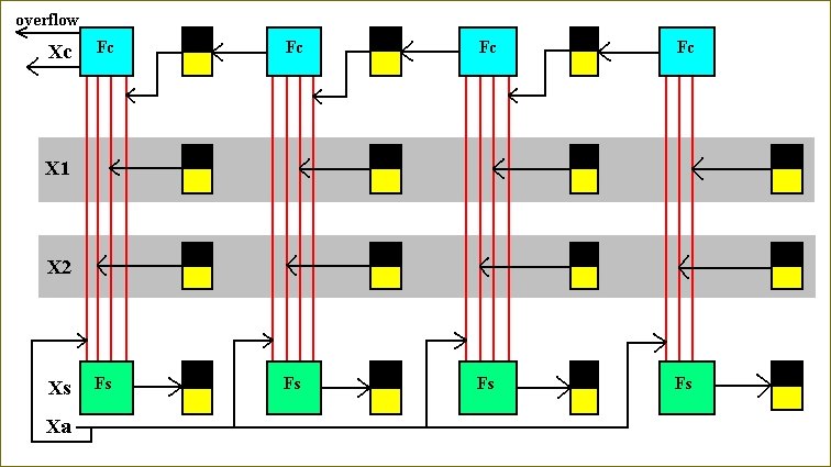
Figure 22. A device for adding the content of two 4-bit registers.
This concludes our exposition of basic computer-circuits, built with relays. The logical design of modern computers (which use transistors instead of relays) is not necessarily the same as that here expounded. The sole purpose was to present some fundamental concepts, that clarify how to " make electricity think ". Only these fundamentals are necessary for an ontological evaluation of Artificial Life creations, for which this Essay forms a preparation.
In order to understand more of the material (i.e. the matter, especially matter as substrate) of modern computers, and to experience some more circuitry, we will treat of transistors. Transistors are electronic switches, that are minute, energy-economic and fast. They form the ' Silicon ' of the modern machines. Thousands of them are integrated in such machines.
In order to understand more of the material (i.e. the matter, especially matter as substrate) of modern computers, and to experience some more circuitry, we will treat of transistors. Transistors are electronic switches, that are minute, energy-economic and fast. They form the ' Silicon ' of the modern machines. Thousands of them are integrated in such machines.
Transistors
Because with transistors we have very small and fast switches, we can integrate them into assemblies consisting of a huge number of them : integrated circuits. Such an integrated circuit will accordingly have small dimensions, thus making the connections very short, which again reduce the time needed for the electrical current to flow across such an integrated circuit, so they become fast, i.e. even very complicated tasks can be executed in a very short time. Let us explain how transistors work.
Electrical Conduction
Materials consist of atoms. Each atom has a nucleus that is surrounded by electrons. These electrons are distributed over so called concentric shells. Each shell can hold a certain maximum number of electrons. Most properties of materials, including electric conductivity, are largely determined by the (number of) electrons in the outermost shell [For atomic structure , see The Essay on the Chemical Bond ]. So in metals, with only one electron in the outermost shell of each of their atoms, it appears that those electrons are not tightly held to their own atoms. They can move freely through the material. So if we make a wire-loop of such material, for example copper, and insert a battery, then an electrical current will develop, because the battery tries (and in this case successfully) to send electrons from its negative pole (symbolized by the shorter outer bar in the symbol for a battery) and to collect them at its other (positive) end (this end is symbolized by the longer bar) :
Some other materials are semiconductors for instance Silicon and Germanium. The arrangement of the atoms of these materials is such that each atom is surrounded by four neighbor atoms. Each atom has four electrons in its outermost shell, and such materials are not necessarily good electrical conductors. Each atom shares these four electrons with its four neighbors. So each atom is surrounded in its outermost shell by these four electrons and one donated (i.e. held commonly) by each of its four neighbors. This form is very stable : The eight electrons are held tightly between the atom cores. Hence no electrons are available for conduction :
Figure 23. A battery applied across a Silicon crystal. The black dots symbolize the Silicon atoms, and the red spots symbolize electrons of their outermost shells. Very little electric current will flow.
But, it turns out that we can engineer the conductivity properties of such a semiconductor. In a Silicon crystal there are no electrons available that can freely move (and will produce a current when an electromotive force -- by means of a battery -- is applied). In other words, we have no carriers . However we could supply such carriers as follows : When, in a Silicon crystal, we replace one Silicon atom by an atom of Phosphorus, then this Phosphorus atom will neatly fit into the crystal-lattice. Phosphorus atoms have five electrons in their outer shell. They share four of them with their Silicon neighbors, but the fifth electron donated by Phosphorus has no stable home and it can be moved by an electromotive force. When we insert, say, several Phosphorus atoms per million Silicon atoms, then their are enough conductor electrons to support an electrical current. Such a Silicon crystal, provided with such ' impurities ', are called n-type doped material, because negative , electrons, are added to achieve conductivity.
Figure 24. A battery applied across an n-type doped Silicon crystal. The extra electrons can support a current.
There are other ways to make crystalline Silicon into a conductor. One such way is to replace some Silicon atoms by Boron atoms. Boron atoms have only three electrons in their outer shell. So when such a Boron atom replaces a Silicon atom, it will try to fit in like the other Silicon atoms among each other. But to do so it misses one electron. We can imagine this missing electron as a hole. These holes can shift from atom to atom causing a net movement of charge. This type of crystal, where the carriers are holes, are called p-type doped material.
Figure 25. A battery applied across a p-type doped Silicon crystal. The holes can migrate from atom to atom (which is the case when an electron from some neighboring atom ' jumps ' into that hole, and leaving behind another hole created by this jumping away) and can accordingly support an electical current.
Thus p-type doped Silicon can be thought of as material with occasional holes here and there where electrons can fit, and n-type doped Silicon is just the opposite, with extra electrons scattered around.
If (material of) the two types are juxtaposed, some of the extra electrons on the n-side will fall across the boundary into holes in the p-side. This means that in the boundary region many carriers (holes on one side of the boundary and free electrons on the other) have disappeared, causing the boundary region poorly-conductive. This can be seen when we apply a battery across the material in the way indicated by Figure 26. In fact the battery will enhance this inconductivity because it fills up the holes above (in the p-type part) and sucks the extra electrons away from below (the n-type part), resulting in the absence of carriers:
If (material of) the two types are juxtaposed, some of the extra electrons on the n-side will fall across the boundary into holes in the p-side. This means that in the boundary region many carriers (holes on one side of the boundary and free electrons on the other) have disappeared, causing the boundary region poorly-conductive. This can be seen when we apply a battery across the material in the way indicated by Figure 26. In fact the battery will enhance this inconductivity because it fills up the holes above (in the p-type part) and sucks the extra electrons away from below (the n-type part), resulting in the absence of carriers:
Figure 26. A battery applied across juxtaposed n-type doped Silicon and p-type doped Silicon. In the direction imposed by the battery only little current can flow through the material.
However, if the battery is reversed, a great change occurs. Now the battery supplies more free electrons into the lower part and sucks electrons away from the upper part, which means that the carriers are constantly being replenished, resulting in good conductivity of the device :
Figure 27. The same as Figure 26, but now with the battery reversed. A good conductivity is the result. A strong electric current is flowing through the device.
What we in fact have constructed is a one-way valve. It allows current only in one direction, the n-p direction. Such a device is called a diode. But what we most need is a device that lets one circuit control another circuit, just like the relays we treated of earlier. Most important is that a low powered circuit can control (i.e. switch on and off) a high(er) powered circuit. So what we need is a kind of switch, analogous to the relay.
Construction of the Transistor
The next step is building a device consisting of three consecuted layers of doped Silicon : A top layer of n-type doped Silicon, called the Collector, a middle layer of p-type doped silicon, called the Base, and a bottom layer of n-type doped Silicon, called the Emitter. When we apply a battery across the emitter-base junction a current will flow, because a current will more easily flow across a n-p junction than it will across a p-n junction :
Figure 28. A small battery applied across the emitter-base junction of a three layered device, made of doped Silicon. A current will flow from the battery through the emitter-base junction, and then back to the (other end of the) battery.
Next let us switch off this ' base current ' and apply a large battery across the whole device :
Figure 29. A large battery applied across a three layered device of doped Silicon of which the base current (from a small battery) is switched off.
Electrons cannot flow from the small battery to the emitter-base junction and back to that battery, because this loop is switched off (it is interrupted by the open switch). So now the current from the large battery will try to flow through the emitter-base junction, but then it encounters a p-n junction, and such a junction will not support current in that direction. Thus there will not flow any current from the large battery through the device and back to that battery, and other possibilities are not present.
But if the small battery is reconnected (by closing the switch), current will flow from the small battery through the emitter-base junction of the device and back into the small battery. So carriers move through the base, and some of these carriers will diffuse across the base-collector junction and consequently will allow it to pass current. Furthermore, in a well designed device (by means of placing some resistors at appropriate places) MOST of the carriers flowing from the emitter will drift into the collector so a rather SUBSTANTIAL current will flow. See Figure 30.
But if the small battery is reconnected (by closing the switch), current will flow from the small battery through the emitter-base junction of the device and back into the small battery. So carriers move through the base, and some of these carriers will diffuse across the base-collector junction and consequently will allow it to pass current. Furthermore, in a well designed device (by means of placing some resistors at appropriate places) MOST of the carriers flowing from the emitter will drift into the collector so a rather SUBSTANTIAL current will flow. See Figure 30.
Figure 30. The same as figure 29, but now with the base current on.
So what we have is the following :
A low powered circuit controlls a high powered circuit : If and when the low powered circuit is ON, current will flow in the high powered circuit, i.e. the high powered circuit is turned ON. If an when the low powered circuit is OFF, there will be no current in the high powered circuit, i.e. the high powered circuit is turned OFF. So the desired switch, built from a doped semiconductor has been constructed. Such a three-layer device is called a transistor. This transistor can be switched ON and OFF by a base current input, and in so doing it can switch ON and OFF a certain circuit.
We now will show how transistors can be used to build computer circuits.
Construction of Transistor-based Computer Circuits
We shall now build a circuit, based on transistor technology, that can compute a useful function :
Figure 31. A transistor-based computer circuit.
The circuit consists of two diodes (n-p junctions), a transistor (n-p-n junction), a few resistors, a small battery Bs and a large battery BL, an output device, that we can imagine being a light bulb, and two input circuits.
Both input circuits, X and Y, should be interpreted as follows : If and when X = 1, the corresponding input circuit has a non-zero voltage and accordingly acts like a battery :
Both input circuits, X and Y, should be interpreted as follows : If and when X = 1, the corresponding input circuit has a non-zero voltage and accordingly acts like a battery :
If and when X = 0, the corresponding input circuit has zero voltage and will act as if it is a simple wire.
Precisely the same applies to input Y.
The analysis that follows will examine the behavior of the circuit assuming each input can have these two behaviors.
The analysis that follows will examine the behavior of the circuit assuming each input can have these two behaviors.
Let us begin by assuming that both inputs are zero, i.e. X = 0 and Y = 0 :
Figure 32. The computer circuit of Figure 31, for X = 0 and Y = 0.
We want to investigate what the output F will be, 1 or 0 (lightbulb on or off).
The electrons from the small battery (Bs) will try to leave the negative end (corresponding to the lowest short bar) and collect again at the positive end of the battery. In so doing they go to the left, flow through both input circuits, through both diodes (i.e. the easy way from n to p) and then, via a small resistor, back to the (small) battery. Because electrical current always takes the easiest route, it will not, after leaving the negative end of the battery, go to the right, go across the emitter-base junction of the transistor and then back to the (small) battery, because this route contains two resistors. This implies that there is no current flowing through the emitter-base junction of the transistor causing the transistor to be OFF. We symbolize this by not drawing the transistor completely, thus emphasizing its non-conductive status.
Next we watch the behavior of the current from the large battery (BL). It will also attempt to force electrons out of its lower wire and collect them at the top. So the current will go to the right, and because the transistor is shut down, it will pass through the output device (the light bulb) and the lamp will be ON, i.e. the output, F, is 1.
So our first result is :
Let us now examine the behavior of the circuit for X = 1 and Y = 0 :
Figure 33. The computer circuit of Figure 31, for X = 1 and Y = 0.
In this case the X input will act like a battery. It will push electrons down its lower wire, but then this current encounters the current from the small battery, Bs, coming from the opposite direction. When we assume that the strenght of the ' battery ' of the X input (the same applies to the Y input when it is on) is the same as that of the small battery, Bs, then it is clear that the two currents, coming from opposite directions, will cancel each other, and this means there will be no current in the upper left region of the circuit. The upper diode consequently does not have any current passing through it, and is drawn as interrupted. But, because Y = 0, the current from the small battery, Bs, is still allowed to pass through the circuit of the Y input and so follow its course through the lower diode and back again to the (small) battery. This is still an easy path, compared with the other alternative path : Going (after leaving the lower end of the small battery, Bs) to the right, then through the emitter-base junction of the transistor and back into the (small) battery, because this path contains two resistors. So the transistor will remain OFF, and the current from the large battery, BL, must go through the output device (the light bulb) and the lamp will remain ON, i.e. F = 1.
So our second result is :
A similar situation occurs when X = 0 and Y = 1 :
Figure 34. The computer circuit of Figure 31, for X = 0 and Y = 1.
Here the easiest path for the current from the small battery, Bs, is through the X input circuit, and then via the diode back to the battery again. So no current is flowing through the emitter-base junction of the transistor, resulting in it to be OFF, implying F = 1.
So our third result is :
Let us finally examine the last possible input-configuration, namely X = 1 and Y = 1 :
Figure 35. The computer circuit of Figure 31, for X = 1 and Y = 1.
In this case the current from the small battery cannot flow to the left, because it is now totally blocked by the two currents from the inputs X and Y (these inputs now both act as if they were batteries). This implies that the current, coming from the lower end of the small battery, Bs, must go to the right and will consequently flow through the emitter-base junction of the transistor causing it to be ON. The transistor can accordingly be drawn just like a line. Therefore the current, coming from the large battery, BL, will take its easiest path through the transistor and then flow back to the positive end of the large battery. It will not flow through the output-device, because this device is in fact a resistor, and therefore this path (through the output-device) will not be the easiest path to follow. So the lamp will go OFF, i.e. F = 0.
So our fourth and final result is :
The analysis of the behavior of the circuit is now complete, and can be summarized in the following function-table :
X    Y         F
----------------
0    0         1
0    1         1
1    0         1
1    1         0
----------------
This circuit is called a NOR circuit, and is symbolized as follows :
Figure 36. Symbol for the NOR circuit.
It is the only building-block needed for constructing all the circuits that were treated of above, using relays :
So the NOT circuit can be built from a NOR circuit by omitting the Y input circuit :
Figure 37. The Transistor-based circuit for computing the NOT-function.
We can symbolize this transistor-based NOT circuit as follows :
Figure 38. Symbol for the NOT circuit.
The function-table for the NOT-function is :
X      F
--------
0      1
1      0
--------
We can construct the AND (transistor-based) circuit by combining the NOR and the NOT circuits, i.e. by negating the output of the NOR circuit, NOT[NOR] = AND, because, when we flip each output of the NOR-function, we get the AND-function :
Figure 39. Symbol for the AND circuit.
The function-table for the AND-function is accordingly :
X    Y         F
----------------
0    0         0
0    1         0
1    0         0
1    1         1
----------------
We can also construct the transistor-based circuit for computing the OR-function. This we do by computing the NOR-function of the negated X and the negated Y, NOR[ NOT[X] NOT[Y] ] :
Figure 40. Symbol for the OR circuit.
This circuit, for computing the OR-function can be determined by showing how to generate the table for the OR-function :
X    Y         F
----------------
0    0         0
0    1         1
1    0         1
1    1         1
----------------
When we compare the output series of this function with that of the NOR-function, we can imagine this output series (of the OR-function) as being the output of some NOR-function. Indeed if we negate X and negate Y, then we get the following values for these negated variables (X and Y) :
NOT[X]  NOT[Y]         F
--------------------------
1       1              0
1       0              1
0       1              1
0       0              1
--------------------------
This is clearly the function NOR[ NOT[X] NOT[Y] ]. And now it is easy to construct the circuit. We take the symbols for NOT[X] and NOT[Y], and make them the elements of a NOR-function (See Figure 40).
The determination of this circuit can be summarized in the following table where the steps are shown together :
The determination of this circuit can be summarized in the following table where the steps are shown together :
X    Y      NOT[X]  NOT[Y]         F (= OR[XY] = NOR[ NOT[X] NOT[Y] ])
------------------------------------
0    0      1       1              0
0    1      1       0              1
1    0      0       1              1
1    1      0       0              1
------------------------------------
Of course we can have a NOR-function with 3 or more variables, for example NOR[XYZ] :
Figure 41. A NOR circuit for three variables X, Y, Z.
The corresponding function-table is :
X    Y     Z            F
-------------------------
0    0     0            1
0    0     1            1
0    1     0            1
0    1     1            1
1    0     0            1
1    0     1            1
1    1     0            1
1    1     1            0
-------------------------
The Transistor-based One-digit Addition Circuit
With our knowledge of transistor-based switches and circuits, we can again construct the circuit that can execute one-digit (binary) addition, but now a transistor-based circuit. One-digit addition means that we confine ourselves to the addition (of two digits) within one column only. We determine the Sum and the Carry. For example, the binary digits 1 and 1 will be added :
1
1
--- +
0 (sum digit)
carry = 1 (carry digit)
1
--- +
0 (sum digit)
carry = 1 (carry digit)
So we need the corresponding functions Fs and Fc, described earlier, defining the sum digit and the carry digit respectively.
Let us start with the function Fs. We want to build (i.e. draw) a transistor-based circuit (using the above symbols) that can compute the function Fs. The table (which was already given earlier), that explicitly defines the Sum (digit), is as follows (Because we assume that the coresponding circuit is turned on, i.e. Xa = 1, we only have to consider the three variables Xc, X1 and X2) :
Let us start with the function Fs. We want to build (i.e. draw) a transistor-based circuit (using the above symbols) that can compute the function Fs. The table (which was already given earlier), that explicitly defines the Sum (digit), is as follows (Because we assume that the coresponding circuit is turned on, i.e. Xa = 1, we only have to consider the three variables Xc, X1 and X2) :
Xc    X1    X2          Fs
--------------------------
0     0     0           0
0     0     1           1
0     1     0           1
0     1     1           0
1     0     0           1
1     0     1           0
1     1     0           0
1     1     1           1
--------------------------
Where Xc is the carry of a previous calculation, X1 the upper digit in the column (formed by the two digits to be added), that should be added to X2, the lower digit in the column.
We now will determine the transistor-based circuit that computes this function.
We see that the last column in the table for Fs contains four 1's. This means that the function returns a 1, if the input is either 001, or 010, or 100, or 111. So we can expect the circuit for this function to consist of four parallel subcircuits. Or, with other words, we can analyse the function Fs into four functions, Fs1, Fs2, Fs3, Fs4, connected to each other by the OR operator :
Xc    X1    X2          Fs1          Fs2          Fs3          Fs4
------------------------------------------------------------------
0     0     0           0            0            0             0
0     0     1           1            0            0             0
0     1     0           0            1            0             0
0     1     1           0            0            0             0
1     0     0           0            0            1             0
1     0     1           0            0            0             0
1     1     0           0            0            0             0
1     1     1           0            0            0             1
------------------------------------------------------------------
We now want to determine the identity of each of the functions Fs1, Fs2, Fs3, and Fs4, i.e. we try to answer the question as to what functions they are. Are they AND-functions, OR-functions, NOT-functions, NOR-functions, or combinations of these?. We start with Fs1.
We determine the identity of the function Fs by constructing a table that analyses the function into simple components. The first three colums of such a table consists of all the possible configurations of the values (0 or 1) of Xc, X1 and X2 :
We determine the identity of the function Fs by constructing a table that analyses the function into simple components. The first three colums of such a table consists of all the possible configurations of the values (0 or 1) of Xc, X1 and X2 :
Xc    X1    X2
--------------
0     0     0
0     0     1
0     1     0
0     1     1
1     0     0
1     0     1
1     1     0
1     1     1
--------------
The next columns (of the table to be constructed) contain values of elementary functions of respectively Xs, X1 and X2. For example when Xc has the value 1, as it is the case in the last four entries of the first column, then NOT[Xc] has the value 0. So NOT[Xc] negates all the values of Xc written down in the first column :
Xc    X1    X2    NOT[Xc]
-------------------------
0     0     0     1
0     0     1     1
0     1     0     1
0     1     1     1
1     0     0     0
1     0     1     0
1     1     0     0
1     1     1     0
-------------------
The same applies to NOT[X1], and also NOT[X2].
These new values we could interpret as inputs for, say, a NOR-function. This function returns a 0, when all input variables have the value 1. It returns a 1 otherwise. We can include this function in the table we are constructing :
These new values we could interpret as inputs for, say, a NOR-function. This function returns a 0, when all input variables have the value 1. It returns a 1 otherwise. We can include this function in the table we are constructing :
Xc    X1    X2    NOT[Xc]    NOT[X1]    NOT[X2]    NOR[ NOT[Xc] NOT[X1] NOT[X2] ]
---------------------------------------------------------------------------------
0     0     0     1          1          1          0
0     0     1     1          1          0          1
0     1     0     1          0          1          1
0     1     1     1          0          0          1
1     0     0     0          1          1          1
1     0     1     0          1          0          1
1     1     0     0          0          1          1
1     1     1     0          0          0          1
-----------------------------------------------------
But we can also leave the value of one or more variables the same, by not applying any function to them (we could equivalently say that we apply to them the identical function, meaning that the values of the input reappear unchanged in the output). For instance we could apply the NOT-function to Xc and to X1, and apply the identical function to X2. And then we could interpret the values of these functions as inputs of the NOR-function :
Xc    X1    X2    NOT[Xc]    NOT[X1]    X2         NOR[ NOT[Xc] NOT[X1] X2 ]
----------------------------------------------------------------------------
0     0     0     1          1          0          1
0     0     1     1          1          1          0
0     1     0     1          0          0          1
0     1     1     1          0          1          1
1     0     0     0          1          0          1
1     0     1     0          1          1          1
1     1     0     0          0          0          1
1     1     1     0          0          1          1
-----------------------------------------------------
When we add another column that writes the NEGATED values of the NOR-column, then we finally get the following table :
Xc  X1  X2  NOT[Xc]  NOT[X1]  X2   NOR[ NOT[Xc] NOT[X1] X2 ]  NOT[ NOR[ NOT[Xc] NOT[X1] X2 ]]
---------------------------------------------------------------------------------------------
0   0   0   1        1        0    1                          0
0   0   1   1        1        1    0                          1
0   1   0   1        0        0    1                          0
0   1   1   1        0        1    1                          0
1   0   0   0        1        0    1                          0
1   0   1   0        1        1    1                          0
1   1   0   0        0        0    1                          0
1   1   1   0        0        1    1                          0
---------------------------------------------------------------
When we look at the values of the last column of this table, then we see in fact the values of the function Fs1, i.e. the first function from the set of four functions (Fs1, Fs2, Fs3, Fs4) obtained by analysing the function Fs. It is now clear that when we want to identify a given function -- given the outputs -- we can, from this given output work backwards to construct a table like the one above, and in this way identify the function, i.e. analyse it in terms of elementary functions.
On the basis of the determined identity of the function Fs1 we can write the transistor-based circuit that computes it :
We now know that when we take the negations of Xc and X1, and X1 as input for the NOR-function, and then negate the obtained values, we will get the output values of the function Fs1. On the basis of this we can construct the corresponding transistor-based circuit :
Figure 42. The circuit that computes the function Fs1.
Now we can, using this method, identify the remaining functions Fs2, Fs3 and Fs4, and determine the transistor-based circuits that computes them (and we know that an OR combination of these four functions is equivalent to the function Fs).
Identification of the function Fs2 :
Identification of the function Fs2 :
Xc  X1  X2  NOT[Xc]  X1  NOT[X2]   NOR[ NOT[Xc] X1 NOT[X2] ]  NOT[ NOR[ NOT[Xc] X1 NOT[X2] ]]
                                                              = Fs2
---------------------------------------------------------------------------------------------
0   0   0   1        0   1         1                          0
0   0   1   1        0   0         1                          0
0   1   0   1        1   1         0                          1
0   1   1   1        1   0         1                          0
1   0   0   0        0   1         1                          0
1   0   1   0        0   0         1                          0
1   1   0   0        1   1         1                          0
1   1   1   0        1   0         1                          0
---------------------------------------------------------------
From this analysis we can determine the circuit that computes the function Fs2 :
Figure 43. The circuit that computes the function Fs2.
Next we will identify the function Fs3, and determine the associated circuit :
Xc  X1  X2  Xc  NOT[X1]  NOT[X2]  NOR[ Xc NOT[X1] NOT[X2] ]  NOT[ NOR[ Xc NOT[X1] NOT[X2] ]]
                                                             = Fs3
--------------------------------------------------------------------------------------------
0   0   0   0   1        1        1                          0
0   0   1   0   1        0        1                          0
0   1   0   0   0        1        1                          0
0   1   1   0   0        0        1                          0
1   0   0   1   1        1        0                          1
1   0   1   1   1        0        1                          0
1   1   0   1   0        1        1                          0
1   1   1   1   0        0        1                          0
--------------------------------------------------------------
The circuit that computes this function is accordingly :
Figure 44. The circuit that computes the function Fs3.
Next we identify the function Fs4 :
Xc  X1  X2     NOR[Xc X1 X2]     NOT[ NOR[Xc X1 X2]]
                                 = Fs4
----------------------------------------------------
0   0   0      1                 0
0   0   1      1                 0
0   1   0      1                 0
0   1   1      1                 0
1   0   0      1                 0
1   0   1      1                 0
1   1   0      1                 0
1   1   1      0                 1
----------------------------------
The associated circuit is accordingly :
Figure 45. The circuit that computes the function Fs4.
These four circuits must now be connected via the OR-function. This we do (see Figure 40) by negate each of these circuits and then connect them via the NOR circuit formed from them :
Figure 46. The circuit that computes the function Fs, but still with some redundant circuitry.
But in this circuit we see four times a set of two NOT-circuits placed after each other. From Logic we know however that when something-negated is again negated it will be affirmed : Peter does not not go to school, means he is going to school.
So two NOT's cancel each other. So the circuit for the function Fs becomes :
So two NOT's cancel each other. So the circuit for the function Fs becomes :
Figure 47. The circuit that computes the function Fs.
For a check, let us fill in Xc = 0, X1 = 0, X2 = 1. According to the function-table of the function Fs the output should be 1.
When we fill in the values of Xc, X1, and X2, into the circuit-diagram, and follow them from left to right, we indeed find that for this set of input-values the output becomes 1 :
When we fill in the values of Xc, X1, and X2, into the circuit-diagram, and follow them from left to right, we indeed find that for this set of input-values the output becomes 1 :
Figure 48. Determination and check of the output of the circuit for Fs, where Xc = 0, X1 = 0, and X2 = 1.
A more convenient way of drawing the circuit-diagram for the function Fs is the following :
Figure 49. The circuit for the function Fs.
This concludes the construction of the transistor-based circuit for computing the function Fs.
Next we must construct the transistor-based circuit that computes the function Fc.
Remember that the functions Fs (sum-bit) and Fc (carry-bit) together constitute the one-bit ADDING function.
Construction of the circuit for Fc.
Again we assume that the circuit that corresponds to Fc is switched on, i.e. Xa = 1 (So we only have to consider the variables Xc, X1, and X2).
By realizing precisely what -- in binary notation -- calculating the value of the carry, when we add two binary digits together (i.e. a one-column addition) actually is, we can construct the table for this carry-function, Fc :
Xc  X1  X2      Fc
------------------
0   0   0       0
0   0   1       0
0   1   0       0
0   1   1       1
1   0   0       0
1   0   1       1
1   1   0       1
1   1   1       1
-----------------
We can dissect this function into four functions (and they are connected by the OR-function). Those functions are Fc1, Fc2, Fc3, Fc4 :
Xc  X1  X2       Fc1      Fc2      Fc3      Fc4
-----------------------------------------------
0   0   0        0        0        0        0
0   0   1        0        0        0        0
0   1   0        0        0        0        0
0   1   1        1        0        0        0
1   0   0        0        0        0        0
1   0   1        0        1        0        0
1   1   0        0        0        1        0
1   1   1        0        0        0        1
---------------------------------------------
Again we analyse these functions into their elementary components in order to determine the circuit that computes them :
Xc  X1  X2    NOT[Xc]  X1  X2   NOR[ NOT[Xc] X1 X2 ]    NOT[ NOR[ NOT[Xc] X1 X2 ]]
                                                        = Fc1
----------------------------------------------------------------------------------
0   0   0    1         0   0    1                       0
0   0   1    1         0   1    1                       0
0   1   0    1         1   0    1                       0
0   1   1    1         1   1    0                       1
1   0   0    0         0   0    1                       0
1   0   1    0         0   1    1                       0
1   1   0    0         1   0    1                       0
1   1   1    0         1   1    1                       0
---------------------------------------------------------
The transistor-based circuit for computing this function is accordingly :
Figure 50. The circuit that computes the function Fc1.
The table for the function Fc2 is :
Xc  X1  X2     Xc  NOT[X1]  X2   NOR[ Xc NOT[X1] X2 ]     NOT[ NOR[ Xc NOT[X1] X2 ]]
                                                          = Fc2
------------------------------------------------------------------------------------
0   0   0      0   1        0    1                        0
0   0   1      0   1        1    1                        0
0   1   0      0   0        0    1                        0
0   1   1      0   0        1    1                        0
1   0   0      1   1        0    1                        0
1   0   1      1   1        1    0                        1
1   1   0      1   0        0    1                        0
1   1   1      1   0        1    1                        0
-----------------------------------------------------------
The transistor-based circuit for computing this function is :
Figure 51. The circuit for computing the function Fc2
The table for the function Fc3 is :
Xc  X1  X2    Xc  X1  NOT[X2]     NOR[ Xc X1 NOT[X2] ]      NOT [ NOR[ Xc X1 NOT[X2] ]]
                                                            = Fc3
---------------------------------------------------------------------------------------
0   0   0     0   0   1           1                         0
0   0   1     0   0   0           1                         0
0   1   0     0   1   1           1                         0
0   1   1     0   1   0           1                         0
1   0   0     1   0   1           1                         0
1   0   1     1   0   0           1                         0
1   1   0     1   1   1           0                         1
1   1   1     1   1   0           1                         0
-------------------------------------------------------------
The transistor-based circuit for computing this function is accordingly :
Figure 52. The circuit for computing the function Fc3.
The table for the function Fc4 is :
Xc  X1  X2       NOR[ Xc X1 X2 ]       NOT[ NOR[ Xc X1 X2 ]]
                                       = Fc4
------------------------------------------------------------
0   0   0        1                     0
0   0   1        1                     0
0   1   0        1                     0
0   1   1        1                     0
1   0   0        1                     0
1   0   1        1                     0
1   1   0        1                     0
1   1   1        0                     1
----------------------------------------
The transistor-based circuit for computing this function is accordingly :
Figure 53. The circuit for computing the function Fc4.
In order to get the complete circuit for the function Fc we must combine these four circuits by means of the OR-function (See Figure 40). This we do by negating the output of each of the functions (Fc1, Fc2, Fc3, Fc4) and then make them the elements of a NOR circuit :
Figure 54. The circuit for the function Fc. There is still some redundancy in the circuit.
Again we see four sets of two negations (NOT-circuits) placed after each other. These will cancel :
Figure 55. The circuit for the function Fc. The redundancy is removed.
This circuit (for the function Fc ) is more conveniently drawn as follows :
Figure 56. The circuit for computing the function Fc
So this finally is the transistor-based circuit for computing the function Fc.
The circuits for Fs and for Fc together form the circuit that can execute one-digit binary addition. The circuits for Fs and Fc have a common input : the values of the three variables Xc, X1, and X2. They are fed into both circuits simultaneously and cause the Fs-circuit to compute the sum-digit, and the Fc-circuit to compute the carry-digit :
Figure 57. The transistor-based circuit for executing one-digit binary addition.
So we now have the complete transistor-based circuit for one-digit binary addition. An input triple (values for Xc, X1, and X2) causes the circuit to compute the sum X1 + X2 and the new carry-value. This new carry-value, Fc, will, in the next calculation -- in case of a more-than-one digit addition -- be attributed to the variable Xc, representing in this next calculation the carry generated by the previous calculation.
When we compare this circuit with the corresponding relay-based circuit, then we see that the NOT-circuits, pictured as

correspond to the relay-based NOT-switches.
correspond to the relay-based NOT-switches.
With the example of a transistor-based circuit that can compute one-digit binary addition, we conclude this section on Transistors.
Transistors and their derivatives provide the millions of switches needed in modern computing machinery. Together they form integrated circuits in such machines.
Transistors and their derivatives provide the millions of switches needed in modern computing machinery. Together they form integrated circuits in such machines.
Basic Design of the Digital Computer
We have learned how to build circuits for computing functions. Now we must find out how all these circuits can work together to constitute a computer. Recall, figures 20 and 21. There we drew a circuit called a recognizer. If and when such a circuit outputs a 1, a certain other circuit -- a computational circuit -- will be switched on. Each computational circuit is in this way associated with a recognizer circuit :
Figure 58. The Instruction Register, Recognizer-circuits and Machine Operation Circuits. Depending on the code in the Instruction Register, a certain Machine Operation Circuit will be switched on.
The Instruction Register, the Recognizer-circuits and the Machine Operation Circuits form a part of the CENTRAL PROCESSING UNIT (CPU) of the computer. Besides this CPU the computer contains a MEMORY BOARD. This board consists of a large amount of storage-circuits. The CPU fetches information (instructions and data) from the MEMORY, executes the instructions on the data, and returns the result to the MEMORY.
The instructions are binary codes and they are sequentially brought into the Instruction Register, IR, of the CPU, and -- sequentially -- executed. A so called Instruction Pointer Register, IP, shows the particular memory address where to find and fetch the particular instruction. When that instruction is fetched and brought (as a copy) into the Instruction Register, the Instruction Pointer Register will indicate the next memory address for fetching the next instruction, as soon as the previous instruction has been carried out. This executing of an instruction is carried out by the appropriate computational circuit -- switched on by the corresponding recognizer circuit. The result of the execution will be placed in another register of the CPU, the Computation Register, AX. The instructions correspond to primitive operations like copying the content of a memeory location into the Computation Register AX of the CPU, or adding the content of a memory location to the content of the Computational Register AX, and leave the result in AX.
Data and instructions normally reside in memory in the form of binary sequences, like 0100, 1100, etc. When a programmer wants the computer to compute something, she must anatomize the desired computation into a set of primitive operations, for which the CPU contains the corresponding circuits. This set of primitive operations to be executed corresponds directly with the set of instructions, instructions which must sequentially loaded into the Instruction Register of the CPU. Because programming with binary sequences is very inconvenient, the programmer uses a (suggestive) name for each instruction. The set of those names and their syntax that must be used to write a computer program is called Assembly Language. The programmer types those names in the required order and those names are immediately translated into machine code, i.e. sequences of 0's and 1's. In our exposition we will not use the binary form of the instructions. Instead of that we represent those binary codes by the Assembly Language expressions placed between asterisks (**). So when the instruction for, say, copying the content of memory location M1 into the Computational Register AX of the CPU, is, say, 0011, then we denote this by :
So COPY AX,M1 is the instruction, while *COPY AX,M1* is its binary code. Also the data are present in the memory in the form of binary sequences : (for example) *7* means 0111, the binary expression for 7.
The CPU-Memory configuration of a simple type of digital computer could look like this (See also BIERMANN, 1990, Great Ideas in Computer Science , pp. 252):
The CPU-Memory configuration of a simple type of digital computer could look like this (See also BIERMANN, 1990, Great Ideas in Computer Science , pp. 252):
Figure 59. Outline of the CPU-Memory configuration of a simple type of digital computer.
The index for the memory location of the instruction *COPY AX, M1* is 10 (of course also coded in binary), and so this instruction will be placed in the Instruction Register IR of the CPU. The Instruction Pointer will now change to the next index, 11. The instruction will be decoded by the mechanism shown in figure 58, which means that the appropriate circuit is turned on. That circuit now executes the instruction COPY AX, M1 and this means that the content of memory location M1 will be copied into the Computation Register AX of the CPU. Now the next instruction, *ADD AX, M2*, is fetched and placed in the Instruction Register, replacing the previous instruction. The Instruction Pointer now sets itself to 12. Decoding and executing the instruction ADD AX, M2 means that the content of memory location M2 is added to the content of AX, and the result (content of M2 + content of AX) remains in AX. Now the next instruction is fetched and placed in the Instruction Register, while the Instruction Pointer goes to 13. This instruction *COPY M3, AX*, will be decoded and executed, resulting in placing the content of AX in memory location M3. Summarizing this all, say we want to add two numbers 8 and 5. The number 8 is present in memory location M1, while the number 5 is in memeory location M2. The result of the addition, 13 (8 + 5), is placed (as *13*) in memory location M3. The Assembly Language program for executing this task was :
ADD AX, M2
COPY M3, AX
Besides the ADD and COPY instructions we will find (circuits for) still other instructions, like MUL (multiply), for example MUL AX, M1, or SUB (subtract), DIV (divide) etc. Other important instructions are of a conditional type. So the instruction CMP that compares two numbers. The result of this comparison will be placed in the Condition Flag, CF. Depending on the outcome of such a comparison either the next index for the memory location will be placed in the Instruction Pointer, resulting in loading the next instruction of the sequence in the Instruction Register, or the Instruction Pointer will jump (i.e. executing a jump-instruction ordered by the program) to another non-consecutive index, causing the machine to jump to an instruction that is not next in the memory sequence. So we could have for instance the instruction CMP AX, M1. This means the following :
If the content of AX is smaller than the content of M1, then the value of the Condition Flag becomes B (CF = B) else the value of the Condition Flag becomes NB (CF = NB). Associated with this condition are two jump-instructions, JNB (jump if not below) and JB (jump if below). JB will be executed if the content of AX is indeed smaller than the content of M1, which causes CF = B. Such a jump-instruction could then be : JB Lab1, which means : Go to the instruction with label lab1 (if CF = B). If the content of AX is not smaller than the content of M1, then CF = NB, and consequently a JNB (jump if not below) instruction will be executed, for example the instruction JNB Lab2, which means : Go to the instruction with label Lab2 (if CF = NB).
Besides these conditional jumps there are also just jumps to be executed. It concerns the instruction JMP (jump), for example JMP Lab3, which means : Go to the instruction with label Lab3.
Thus after such a jump the machine starts to follow (i.e. fetch, decode and execute) a new sequence (in memory) of instructions, or, the same sequence all over again.
We already gave an Assembly Language program for adding numbers. Another example of such a program could be one that computes the absolute value of a given number, i.e. it outputs that same number if it is positive, and outputs its negative if it is negative [ The number to be manipulated is assumed to reside in memory location M1. To output the result -- print it as program output on screen or printer -- is taken care of by the instruction OUT AX. The sign := means gets the value of. ] :
PROGRAM                 NUMERICAL EXAMPLE  (M1 contains the number  -5 )

-------------------------------------------------------------------------------------------
      COPY  AX, M1      AX := -5

      SUB  AX, M1       -5 - (-5) = 0 (i.e. AX := 0)

      CMP  AX, M1       0 is not below -5, CF := NB, therefore the JB instruction is skipped

      JB  NEXT          If AX is below M1 then go to the instruction with label NEXT

      SUB  AX, M1       0 - (-5) = 5 (i.e. AX := 5)

      COPY  M1, AX      M1 := 5

NEXT  COPY  AX, M1      AX := 5

      OUT  AX           print 5

-------------------------------------------------------------------------------------------
If the number in M1 was 5, then we get :
AX := 5
5 - 5 = 0 (i.e. AX := 0)
0 is below 5, CF := B, thus the instruction JB (jump if below) must be followed, so the machine must go to the instruction with the label NEXT.
AX := 5
print 5
5 - 5 = 0 (i.e. AX := 0)
0 is below 5, CF := B, thus the instruction JB (jump if below) must be followed, so the machine must go to the instruction with the label NEXT.
AX := 5
print 5
A processor of a computer contains a number of circuits, among them a set of computational circuits. Depending on, and corresponding with, this set, the processor supports a fixed series of different types of instructions. The programmer (programming in Assembly Language) must select a subset from these available (basic) instructions to compose his computer program. He first thinks about a verbal solution to the problem he wants the computer to solve, the algorithm. Then he tries to translate this algorithm into a sequence of the available basic instructions supported by the processor, i.e. he tries to translate his algorithm into Assembly Language. He accordingly obtains a computer program that can be implemented on the computer (with that particular type of processor), i.e. the Assembly program lines are typed in and directly translated into the corresponding binary codes. These codes will now reside in memory, and can sequentially be brought into the Instruction Register of that processor (CPU).
Even in Assembly Language it is not easy programming because every task must be anatomized into the basic instructions, i.e. the task must be expressed in terms of these elementary instructions like COPY AX, M2. In order to be able to program a computer more conveniently, so called higher programming languages have been created, like for instance the programming language PASCAL. Within this language we can write on a higher level than the level of elementary machine instructions. Along with such a higher language one has developed translators, programs that translate lines of a program written in a higher programming language into basic machine code. The existence and use of such higher programming languages and their associated translators, are not important for our (philosophical) purpose. For investigating the ontological status of a running digital computer it is sufficient to consider the program in machine code (or, as one wishes, in Assembly Language) and contemplate its execution. Each Assembly Language instruction, like ADD AX, M5, COPY AX, M1, etc. corresponds to a certain electrical circuit. These circuits, together with the storage circuits, constitute the interacting elements of the computer when it is interpreted as a dynamical system.
Even in Assembly Language it is not easy programming because every task must be anatomized into the basic instructions, i.e. the task must be expressed in terms of these elementary instructions like COPY AX, M2. In order to be able to program a computer more conveniently, so called higher programming languages have been created, like for instance the programming language PASCAL. Within this language we can write on a higher level than the level of elementary machine instructions. Along with such a higher language one has developed translators, programs that translate lines of a program written in a higher programming language into basic machine code. The existence and use of such higher programming languages and their associated translators, are not important for our (philosophical) purpose. For investigating the ontological status of a running digital computer it is sufficient to consider the program in machine code (or, as one wishes, in Assembly Language) and contemplate its execution. Each Assembly Language instruction, like ADD AX, M5, COPY AX, M1, etc. corresponds to a certain electrical circuit. These circuits, together with the storage circuits, constitute the interacting elements of the computer when it is interpreted as a dynamical system.
Ontological Interpretation of the Digital Computer
In Part One we discussed the UNIVERSAL TURING MACHINE.
As such this " machine " is not yet a machine, not yet a -- physical -- computer, but just the BARE CONCEPT of a digital computing machine.
In Part Two we have PHYSICALLY EMBODIED this concept by means of the design of electrical circuits, that can actually be constructed from real materials like copper and doped semi-conductor materials.
Only if and when we have actually constructed such a machine by means of those circuits, we have a physical digital computer.
Such a physical computer can be interpreted as a COMPLEX DYNAMICAL SYSTEM. Its interacting elements are its elementary circuits :
A circuit A can receive input from (the output of) circuit B. Circuit B can be either a storage-circuit, or a computational-circuit. The output of this circuit is input for circuit A and could modify its output. This output could itself become the input for circuit A, i.e. for itself, or for another circuit, say, C, or it could be the input for circuit B. So the circuits are interacting with each other, like people in a society, and will give rise to an overall output of the computing machine. When complex interactions take place in such a machine, emergent behavior is to be expected. But all this remains a bottom-up process. These emergent behaviors can play a role in Artificial Life research, but the question whether these behaviors are in some cases ' alive ' or not, is in fact irrelevant for the assessment of the ontological status of those behaviors. The machine can behave in complex ways that we decide to call living. The basic elements of such an artificial life system are the circuits of the physical computer, that is, (only) those circuits that participate directly in the relevant emergent behaviors (i.e. are directly -- be it all the way from the bottom -- responsible for generating them). So computer-based artificial life is a physical process, a physical dynamical system, but its elements are not (macro-) molecules, but (elementary) circuits. Ultimately however the elements are atoms and free electrons.
XO___XO Microprocessor Programming
The “vocabulary” of instructions which any particular microprocessor chip possesses is specific to that model of chip. An Intel 80386, for example, uses a completely different set of binary codes than a Motorola 68020, for designating equivalent functions. Unfortunately, there are no standards in place for microprocessor instructions. This makes programming at the very lowest level very confusing and specialized.
When a human programmer develops a set of instructions to directly tell a microprocessor how to do something (like automatically control the fuel injection rate to an engine), they’re programming in the CPU’s own “language.” This language, which consists of the very same binary codes which the Control Unit inside the CPU chip decodes to perform tasks, is often referred to as machine language. While machine language software can be “worded” in binary notation, it is often written in hexadecimal form, because it is easier for human beings to work with. For example, I’ll present just a few of the common instruction codes for the Intel 8080 micro-processor chip:
Hexadecimal    Binary              Instruction description
-----------   --------   -----------------------------------------
|   7B        01111011   Move contents of register A to register E
|
|   87        10000111   Add contents of register A to register D
|
|   1C        00011100   Increment the contents of register E by 1
|
|   D3        11010011   Output byte of data to data bus
Even with hexadecimal notation, these instructions can be easily confused and forgotten. For this purpose, another aid for programmers exists called assembly language. With assembly language, two to four letter mnemonic words are used in place of the actual hex or binary code for describing program steps. For example, the instruction 7B for the Intel 8080 would be “MOV A,E” in assembly language. The mnemonics, of course, are useless to the microprocessor, which can only understand binary codes, but it is an expedient way for programmers to manage the writing of their programs on paper or text editor (word processor). There are even programs written for computers called assemblers which understand these mnemonics, translating them to the appropriate binary codes for a specified target microprocessor, so that the programmer can write a program in the computer’s native language without ever having to deal with strange hex or tedious binary code notation.
Once a program is developed by a person, it must be written into memory before a microprocessor can execute it. If the program is to be stored in ROM (which some are), this can be done with a special machine called a ROM programmer, or (if you’re masochistic), by plugging the ROM chip into a breadboard, powering it up with the appropriate voltages, and writing data by making the right wire connections to the address and data lines, one at a time, for each instruction. If the program is to be stored in volatile memory, such as the operating computer’s RAM memory, there may be a way to type it in by hand through that computer’s keyboard (some computers have a mini-program stored in ROM which tells the microprocessor how to accept keystrokes from a keyboard and store them as commands in RAM), even if it is too dumb to do anything else. Many “hobby” computer kits work like this. If the computer to be programmed is a fully-functional personal computer with an operating system, disk drives, and the whole works, you can simply command the assembler to store your finished program onto a disk for later retrieval. To “run” your program, you would simply type your program’s filename at the prompt, press the Enter key, and the microprocessor’s Program Counter register would be set to point to the location (“address”) on the disk where the first instruction is stored, and your program would run from there.
Although programming in machine language or assembly language makes for fast and highly efficient programs, it takes a lot of time and skill to do so for anything but the simplest tasks, because each machine language instruction is so crude. The answer to this is to develop ways for programmers to write in “high level” languages, which can more efficiently express human thought. Instead of typing in dozens of cryptic assembly language codes, a programmer writing in a high-level language would be able to write something like this . . .
Print "Hello, world!"
. . . and expect the computer to print “Hello, world!” with no further instruction on how to do so. This is a great idea, but how does a microprocessor understand such “human” thinking when its vocabulary is so limited?
The answer comes in two different forms: interpretation, or compilation. Just like two people speaking different languages, there has to be some way to transcend the language barrier in order for them to converse. A translator is needed to translate each person’s words to the other person’s language, one way at a time. For the microprocessor, this means another program, written by another programmer in machine language, which recognizes the ASCII character patterns of high-level commands such as Print (P-r-i-n-t) and can translate them into the necessary bite-size steps that the microprocessor can directly understand. If this translation is done during program execution, just like a translator intervening between two people in a live conversation, it is called “interpretation.” On the other hand, if the entire program is translated to machine language in one fell swoop, like a translator recording a monologue on paper and then translating all the words at one sitting into a written document in the other language, the process is called “compilation.”
Interpretation is simple, but makes for a slow-running program because the microprocessor has to continually translate the program between steps, and that takes time. Compilation takes time initially to translate the whole program into machine code, but the resulting machine code needs no translation after that and runs faster as a consequence. Programming languages such as BASIC and FORTH are interpreted. Languages such as C, C++, FORTRAN, and PASCAL are compiled. Compiled languages are generally considered to be the languages of choice for professional programmers, because of the efficiency of the final product.
Naturally, because machine language vocabularies vary widely from microprocessor to microprocessor, and since high-level languages are designed to be as universal as possible, the interpreting and compiling programs necessary for language translation must be microprocessor-specific. Development of these interpreters and compilers is a most impressive feat: the people who make these programs most definitely earn their keep, especially when you consider the work they must do to keep their software product current with the rapidly-changing microprocessor models appearing on the market!
To mitigate this difficulty, the trend-setting manufacturers of microprocessor chips (most notably, Intel and Motorola) try to design their new products to be backwardly compatible with their older products. For example, the entire instruction set for the Intel 80386 chip is contained within the latest Pentium IV chips, although the Pentium chips have additional instructions that the 80386 chips lack. What this means is that machine-language programs (compilers, too) written for 80386 computers will run on the latest and greatest Intel Pentium IV CPU, but machine-language programs written specifically to take advantage of the Pentium’s larger instruction set will not run on an 80386, because the older CPU simply doesn’t have some of those instructions in its vocabulary: the Control Unit inside the 80386 cannot decode them.
Building on this theme, most compilers have settings that allow the programmer to select which CPU type he or she wants to compile machine-language code for. If they select the 80386 setting, the compiler will perform the translation using only instructions known to the 80386 chip; if they select the Pentium setting, the compiler is free to make use of all instructions known to Pentiums. This is analogous to telling a translator what minimum reading level their audience will be: a document translated for a child will be .
In digital circuitry, however, there are only two states: on and off, also referred to as 1 and 0, respectively. Digital information has its roots back in the Victorian era thanks to George Boole, who developed the idea of Boolean algebra.
Every aspect of our lives is increasingly becoming integrated and connected by the Internet of Things (IoT), which consists of computers and embedded systems. These devices are controlled by software which at its core is Boolean logic in conjunction with digital information. The world around us is analogue, but with every passing day our interaction with the world is becoming more digital and more integrated.
Suppose we wanted to build a device that could add two binary bits together. Such a device is known as a half-adder, and its gate circuit looks like this:
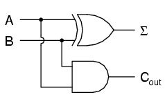
The Σ symbol represents the “sum” output of the half-adder, the sum’s least significant bit (LSB). Coutrepresents the “carry” output of the half-adder, the sum’s most significant bit (MSB).
If we were to implement this same function in ladder (relay) logic, it would look like this:
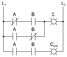
Either circuit is capable of adding two binary digits together. The mathematical “rules” of how to add bits together are intrinsic to the hard-wired logic of the circuits. If we wanted to perform a different arithmetic operation with binary bits, such as multiplication, we would have to construct another circuit. The above circuit designs will only perform one function: add two binary bits together. To make them do something else would take re-wiring, and perhaps different componentry.
In this sense, digital arithmetic circuits aren’t much different from analog arithmetic (operational amplifier) circuits: they do exactly what they’re wired to do, no more and no less. We are not, however, restricted to designing digital computer circuits in this manner. It is possible to embed the mathematical “rules” for any arithmetic operation in the form of digital data rather than in hard-wired connections between gates. The result is unparalleled flexibility in operation, giving rise to a whole new kind of digital device: the programmable computer.
While this chapter is by no means exhaustive, it provides what I believe is a unique and interesting look at the nature of programmable computer devices, starting with two devices often overlooked in introductory textbooks: look-up table memories and finite-state machines.
XO___XO DW Pascal - Operators
An operator is a symbol that tells the compiler to perform specific mathematical or logical manipulations. Pascal allows the following types of operators −
- Arithmetic operators
- Relational operators
- Boolean operators
- Bit operators
- Set operators
- String operators
Let us discuss the arithmetic, relational, Boolean and bit operators one by one. We will discuss the set operators and string operations later.
Arithmetic Operators
Following table shows all the arithmetic operators supported by Pascal. Assume variable A holds 10 and variable B holds 20, then −
| Operator | Description | Example |
|---|---|---|
| + | Adds two operands | A + B will give 30 |
| - | Subtracts second operand from the first | A - B will give -10 |
| * | Multiplies both operands | A * B will give 200 |
| / | Divides numerator by denominator | B / A will give 2 |
| % | Modulus Operator and remainder of after an integer division | B % A will give 0 |
Relational Operators
Following table shows all the relational operators supported by Pascal. Assume variable A holds 10 and variable B holds 20, then −
| Operator | Description | Example |
|---|---|---|
| = | Checks if the values of two operands are equal or not, if yes, then condition becomes true. | (A = B) is not true. |
| <> | Checks if the values of two operands are equal or not, if values are not equal, then condition becomes true. | (A <> B) is true. |
| > | Checks if the value of left operand is greater than the value of right operand, if yes, then condition becomes true. | (A > B) is not true. |
| < | Checks if the value of left operand is less than the value of right operand, if yes, then condition becomes true. | (A < B) is true. |
| >= | Checks if the value of left operand is greater than or equal to the value of right operand, if yes, then condition becomes true. | (A >= B) is not true. |
| <= | Checks if the value of left operand is less than or equal to the value of right operand, if yes, then condition becomes true. | (A <= B) is true. |
Boolean Operators
Following table shows all the Boolean operators supported by Pascal language. All these operators work on Boolean operands and produce Boolean results. Assume variable A holds true and variable B holds false, then −
| Operator | Description | Example |
|---|---|---|
| and | Called Boolean AND operator. If both the operands are true, then condition becomes true. | (A and B) is false. |
| and then | It is similar to the AND operator, however, it guarantees the order in which the compiler evaluates the logical expression. Left to right and the right operands are evaluated only when necessary. | (A and then B) is false. |
| or | Called Boolean OR Operator. If any of the two operands is true, then condition becomes true. | (A or B) is true. |
| or else | It is similar to Boolean OR, however, it guarantees the order in which the compiler evaluates the logical expression. Left to right and the right operands are evaluated only when necessary. | (A or else B) is true. |
| not | Called Boolean NOT Operator. Used to reverse the logical state of its operand. If a condition is true, then Logical NOT operator will make it false. | not (A and B) is true. |
Bit Operators
Bitwise operators work on bits and perform bit-by-bit operation. All these operators work on integer operands and produces integer results. The truth table for bitwise and (&), bitwise or (|), and bitwise not (~) are as follows −
| p | q | p & q | p | q | ~p | ~q |
|---|---|---|---|---|---|
| 0 | 0 | 0 | 0 | 1 | 1 |
| 0 | 1 | 0 | 1 | 1 | 0 |
| 1 | 1 | 1 | 1 | 0 | 0 |
| 1 | 0 | 0 | 1 | 0 | 1 |
Assume if A = 60; and B = 13; now in binary format they will be as follows −
A = 0011 1100
B = 0000 1101
-----------------
A&B = 0000 1100
A^B = 0011 0001
~A = 1100 0011
The Bitwise operators supported by Pascal are listed in the following table. Assume variable A holds 60 and variable B holds 13, then:
| Operator | Description | Example |
|---|---|---|
| & | Binary AND Operator copies a bit to the result if it exists in both operands. | (A & B) will give 12, which is 0000 1100 |
| | | Binary OR Operator copies a bit if it exists in either operand. | (A | B) will give 61, which is 0011 1101 |
| ! | Binary OR Operator copies a bit if it exists in either operand. Its same as | operator. | (A ! B) will give 61, which is 0011 1101 |
| ~ | Binary Ones Complement Operator is unary and has the effect of 'flipping' bits. | (~A ) will give -61, which is 1100 0011 in 2's complement form due to a signed binary number. |
| << | Binary Left Shift Operator. The left operands value is moved left by the number of bits specified by the right operand. | A << 2 will give 240, which is 1111 0000 |
| >> | Binary Right Shift Operator. The left operands value is moved right by the number of bits specified by the right operand. | A >> 2 will give 15, which is 0000 1111 |
Please note that different implementations of Pascal differ in bitwise operators. Free Pascal, the compiler we used here, however, supports the following bitwise operators −
| Operators | Operations |
|---|---|
| not | Bitwise NOT |
| and | Bitwise AND |
| or | Bitwise OR |
| xor | Bitwise exclusive OR |
| shl | Bitwise shift left |
| shr | Bitwise shift right |
| << | Bitwise shift left |
| >> | Bitwise shift right |
Operators Precedence in Pascal
Operator precedence determines the grouping of terms in an expression. This affects how an expression is evaluated. Certain operators have higher precedence than others; for example, the multiplication operator has higher precedence than the addition operator.
For example x = 7 + 3 * 2; here, x is assigned 13, not 20 because operator * has higher precedence than +, so it first gets multiplied with 3*2 and then adds into 7.
Here, operators with the highest precedence appear at the top of the table, those with the lowest appear at the bottom. Within an expression, higher precedence operators will be evaluated first.
| Operator | Precedence |
|---|---|
| ~, not, | Highest |
| *, /, div, mod, and, & | |
| |, !, +, -, or, | |
| =, <>, <, <=, >, >=, in | |
| or else, and then | Lowest |
Pascal - Decision Making
Decision making structures require that the programmer specify one or more conditions to be evaluated or tested by the program, along with a statement or statements to be executed if the condition is determined to be true, and optionally, other statements to be executed if the condition is determined to be false.
Following is the general form of a typical decision making structure found in most of the programming languages −
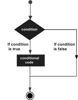
Pascal programming language provides the following types of decision making statements. Click the following links to check their detail.
| Sr.No | Statement & Description |
|---|---|
| 1 | if - then statement
An if - then statement consists of a boolean expression followed by one or more statements.
|
| 2 | If-then-else statement
An if - then statement can be followed by an optional else statement, which executes when the boolean expression is false.
|
| 3 | nested if statements
You can use one if or else if statement inside another if or else if statement(s).
|
| 4 | case statement
A case statement allows a variable to be tested for equality against a list of values.
|
| 5 | case - else statement
It is similar to the if-then-else statement. Here, an else term follows the case statement.
|
| 6 | nested case statements
You can use one case statement inside another case statement(s).
|
Pascal - Loops
There may be a situation, when you need to execute a block of code several number of times. In general, statements are executed sequentially: The first statement in a function is executed first, followed by the second, and so on.
Programming languages provide various control structures that allow for more complicated execution paths.
A loop statement allows us to execute a statement or group of statements multiple times and following is the general form of a loop statement in most of the programming languages −
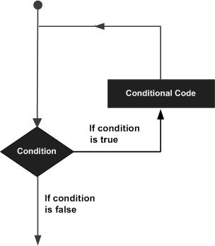
Pascal programming language provides the following types of loop constructs to handle looping requirements. Click the following links to check their details.
| Sr.No | Loop Type & Description |
|---|---|
| 1 | while-do loop
Repeats a statement or group of statements while a given condition is true. It tests the condition before executing the loop body.
|
| 2 | for-do loop
Executes a sequence of statements multiple times and abbreviates the code that manages the loop variable.
|
| 3 | repeat-until loop
Like a while statement, except that it tests the condition at the end of the loop body.
|
| 4 | nested loops
You can use one or more loop inside any another while, for or repeat until loop.
|
Loop Control Statements
Loop control statements change execution from its normal sequence. When execution leaves a scope, all automatic objects that were created in that scope are destroyed.
Pascal supports the following control statements. Click the following links to check their details.
| Sr.No | Control Statement & Description |
|---|---|
| 1 | break statement
Terminates the loop or case statement and transfers execution to the statement immediately following the loop or case statement.
|
| 2 | continue statement
Causes the loop to skip the remainder of its body and immediately retest its condition prior to reiterating.
|
| 3 | goto statement
Transfers control to the labeled statement. Though it is not advised to use goto statement in your program.
|
Pascal - Functions
Subprograms
A subprogram is a program unit/module that performs a particular task. These subprograms are combined to form larger programs. This is basically called the 'Modular design.' A subprogram can be invoked by a subprogram/program, which is called the calling program.
Pascal provides two kinds of subprograms −
- Functions − these subprograms return a single value.
- Procedures − these subprograms do not return a value directly.
Functions
A function is a group of statements that together perform a task. Every Pascal program has at least one function, which is the program itself, and all the most trivial programs can define additional functions.
A function declaration tells the compiler about a function's name, return type, and parameters. A function definition provides the actual body of the function.
Pascal standard library provides numerous built-in functions that your program can call. For example, function AppendStr() appends two strings, function New() dynamically allocates memory to variables and many more functions.
Defining a Function
In Pascal, a function is defined using the function keyword. The general form of a function definition is as follows −
function name(argument(s): type1; argument(s): type2; ...): function_type;
local declarations;

begin
   ...
   < statements >
   ...
   name:= expression;
end;
A function definition in Pascal consists of a function header, local declarations and a function body. The function header consists of the keyword function and a name given to the function. Here are all the parts of a function −
- Arguments − The argument(s) establish the linkage between the calling program and the function identifiers and also called the formal parameters. A parameter is like a placeholder. When a function is invoked, you pass a value to the parameter. This value is referred to as actual parameter or argument. The parameter list refers to the type, order, and number of parameters of a function. Use of such formal parameters is optional. These parameters may have standard data type, user-defined data type or subrange data type.The formal parameters list appearing in the function statement could be simple or subscripted variables, arrays or structured variables, or subprograms.
- Return Type − All functions must return a value, so all functions must be assigned a type. The function-type is the data type of the value the function returns. It may be standard, user-defined scalar or subrange type but it cannot be structured type.
- Local declarations − Local declarations refer to the declarations for labels, constants, variables, functions and procedures, which are application to the body of function only.
- Function Body − The function body contains a collection of statements that define what the function does. It should always be enclosed between the reserved words begin and end. It is the part of a function where all computations are done. There must be an assignment statement of the type - name := expression; in the function body that assigns a value to the function name. This value is returned as and when the function is executed. The last statement in the body must be an end statement.
Following is an example showing how to define a function in pascal −
(* function returning the max between two numbers *)
function max(num1, num2: integer): integer;

var
   (* local variable declaration *)
   result: integer;

begin
   if (num1 > num2) then
      result := num1

   else
      result := num2;
   max := result;
end;
Function Declarations
A function declaration tells the compiler about a function name and how to call the function. The actual body of the function can be defined separately.
A function declaration has the following parts −
function name(argument(s): type1; argument(s): type2; ...): function_type;
For the above-defined function max(), following is the function declaration −
function max(num1, num2: integer): integer;
Function declaration is required when you define a function in one source file and you call that function in another file. In such case, you should declare the function at the top of the file calling the function.
Calling a Function
While creating a function, you give a definition of what the function has to do. To use a function, you will have to call that function to perform the defined task. When a program calls a function, program control is transferred to the called function. A called function performs defined task, and when its return statement is executed or when it last end statement is reached, it returns program control back to the main program.
To call a function, you simply need to pass the required parameters along with function name, and if function returns a value, then you can store returned value. Following is a simple example to show the usage −
Live Demoprogram exFunction; var a, b, ret : integer; (*function definition *) function max(num1, num2: integer): integer; var (* local variable declaration *) result: integer; begin if (num1 > num2) then result := num1 else result := num2; max := result; end; begin a := 100; b := 200; (* calling a function to get max value *) ret := max(a, b); writeln( 'Max value is : ', ret ); end.
When the above code is compiled and executed, it produces the following result −
Pascal - Procedures
Procedures are subprograms that, instead of returning a single value, allow to obtain a group of results.
Defining a Procedure
In Pascal, a procedure is defined using the procedure keyword. The general form of a procedure definition is as follows −
procedure name(argument(s): type1, argument(s): type 2, ... );
   < local declarations >
begin
   < procedure body >
end;
A procedure definition in Pascal consists of a header, local declarations and a body of the procedure. The procedure header consists of the keyword procedure and a name given to the procedure. Here are all the parts of a procedure −
- Arguments − The argument(s) establish the linkage between the calling program and the procedure identifiers and also called the formal parameters. Rules for arguments in procedures are same as that for the functions.
- Local declarations − Local declarations refer to the declarations for labels, constants, variables, functions and procedures, which are applicable to the body of the procedure only.
- Procedure Body − The procedure body contains a collection of statements that define what the procedure does. It should always be enclosed between the reserved words begin and end. It is the part of a procedure where all computations are done.
Following is the source code for a procedure called findMin(). This procedure takes 4 parameters x, y, z and m and stores the minimum among the first three variables in the variable named m. The variable m is passed by reference (we will discuss passing arguments by reference a little later) −
procedure findMin(x, y, z: integer; var m: integer);
(* Finds the minimum of the 3 values *)

begin
   if x < y then
      m := x
   else
      m := y;

   if z <m then
      m := z;
end; { end of procedure findMin }
Procedure Declarations
A procedure declaration tells the compiler about a procedure name and how to call the procedure. The actual body of the procedure can be defined separately.
A procedure declaration has the following syntax −
procedure name(argument(s): type1, argument(s): type 2, ... );
Please note that the name of the procedure is not associated with any type. For the above defined procedure findMin(), following is the declaration −
procedure findMin(x, y, z: integer; var m: integer);
Calling a Procedure
While creating a procedure, you give a definition of what the procedure has to do. To use the procedure, you will have to call that procedure to perform the defined task. When a program calls a procedure, program control is transferred to the called procedure. A called procedure performs the defined task, and when its last end statement is reached, it returns the control back to the calling program.
To call a procedure, you simply need to pass the required parameters along with the procedure name as shown below −
program exProcedure;
var
   a, b, c,  min: integer;
procedure findMin(x, y, z: integer; var m: integer);
(* Finds the minimum of the 3 values *)

begin
   if x < y then
      m:= x
   else
      m:= y;

   if z < m then
      m:= z;
end; { end of procedure findMin }

begin
   writeln(' Enter three numbers: ');
   readln( a, b, c);
   findMin(a, b, c, min); (* Procedure call *)

   writeln(' Minimum: ', min);
end.
When the above code is compiled and executed, it produces the following result −
Enter three numbers:
89 45 67
Minimum: 45
Recursive Subprograms
We have seen that a program or subprogram may call another subprogram. When a subprogram calls itself, it is referred to as a recursive call and the process is known as recursion.
To illustrate the concept, let us calculate the factorial of a number. Factorial of a number n is defined as −
n! = n*(n-1)!
   = n*(n-1)*(n-2)!
      ...
   = n*(n-1)*(n-2)*(n-3)... 1
The following program calculates the factorial of a given number by calling itself recursively.
program exRecursion;
var
   num, f: integer;
function fact(x: integer): integer; (* calculates factorial of x - x! *)

begin
   if x=0 then
      fact := 1
   else
      fact := x * fact(x-1); (* recursive call *)
end; { end of function fact}

begin
   writeln(' Enter a number: ');
   readln(num);
   f := fact(num);

   writeln(' Factorial ', num, ' is: ' , f);
end.
When the above code is compiled and executed, it produces the following result −
Enter a number:
5
Factorial 5 is: 120
Following is another example, which generates the Fibonacci Series for a given number using a recursive function −
program recursiveFibonacci;
var
   i: integer;
function fibonacci(n: integer): integer;

begin
   if n=1 then
      fibonacci := 0

   else if n=2 then
      fibonacci := 1

   else
      fibonacci := fibonacci(n-1) + fibonacci(n-2);
end;

begin
   for i:= 1 to 10 do

   write(fibonacci (i), '  ');
end.
When the above code is compiled and executed, it produces the following result −
0 1 1 2 3 5 8 13 21 34
Arguments of a Subprogram
If a subprogram (function or procedure) is to use arguments, it must declare variables that accept the values of the arguments. These variables are called the formal parameters of the subprogram.
The formal parameters behave like other local variables inside the subprogram and are created upon entry into the subprogram and destroyed upon exit.
While calling a subprogram, there are two ways that arguments can be passed to the subprogram −
| Sr.No | Call Type & Description |
|---|---|
| 1 | Call by value
This method copies the actual value of an argument into the formal parameter of the subprogram. In this case, changes made to the parameter inside the subprogram have no effect on the argument.
|
| 2 | Call by reference
This method copies the address of an argument into the formal parameter. Inside the subprogram, the address is used to access the actual argument used in the call. This means that changes made to the parameter affect the argument.
|
By default, Pascal uses call by value to pass arguments. In general, this means that code within a subprogram cannot alter the arguments used to call the subprogram. The example program we used in the chapter 'Pascal - Functions' called the function named max() using call by value.
Whereas, the example program provided here (exProcedure) calls the procedure findMin() using call by reference.
Pascal - Date and Time
Most of the softwares you write need implementing some form of date functions returning current date and time. Dates are so much part of everyday life that it becomes easy to work with them without thinking. Pascal also provides powerful tools for date arithmetic that makes manipulating dates easy. However, the actual name and workings of these functions are different for different compilers.
Getting the Current Date & Time
Pascal's TimeToString function gives you the current time in a colon(: ) delimited form. The following example shows how to get the current time −
Live Demoprogram TimeDemo; uses sysutils; begin writeln ('Current time : ',TimeToStr(Time)); end.
When the above code was compiled and executed, it produces the following result −
Current time : 18:33:08
The Date function returns the current date in TDateTime format. The TDateTime is a double value, which needs some decoding and formatting. The following program demonstrates how to use it in your program to display the current date −
Program DateDemo;
uses sysutils;
var
   YY,MM,DD : Word;

begin
   writeln ('Date : ',Date);
   DeCodeDate (Date,YY,MM,DD);
   writeln (format ('Today is (DD/MM/YY): %d/%d/%d ',[dd,mm,yy]));
end.
When the above code was compiled and executed, it produces the following result −
Date: 4.111300000000000E+004
Today is (DD/MM/YY):23/7/2012
The Now function returns the current date and time −
Live DemoProgram DatenTimeDemo; uses sysutils; begin writeln ('Date and Time at the time of writing : ',DateTimeToStr(Now)); end.
When the above code was compiled and executed, it produces the following result −
Date and Time at the time of writing : 23/7/2012 18:51:
Free Pascal provides a simple time stamp structure named TTimeStamp, which has the following format −
type TTimeStamp = record
   Time: Integer;
   Date: Integer;
end;
Various Date & Time Functions
Free Pascal provides the following date and time functions −
| Sr.No. | Function Name & Description |
|---|---|
| 1 |
function DateTimeToFileDate(DateTime: TDateTime):LongInt;
Converts DateTime type to file date.
|
| 2 |
function DateTimeToStr( DateTime: TDateTime):;
Constructs string representation of DateTime
|
| 3 |
function DateTimeToStr(DateTime: TDateTime; const FormatSettings: TFormatSettings):;
Constructs string representation of DateTime
|
| 4 |
procedure DateTimeToString(out Result: ;const FormatStr: ;const DateTime: TDateTime);
Constructs string representation of DateTime
|
| 5 |
procedure DateTimeToString(out Result: ; const FormatStr: ; const DateTime: TDateTime; const FormatSettings: TFormatSettings);
Constructs string representation of DateTime
|
| 6 |
procedure DateTimeToSystemTime(DateTime: TDateTime; out SystemTime: TSystemTime);
Converts DateTime to system time
|
| 7 |
function DateTimeToTimeStamp( DateTime: TDateTime):TTimeStamp;Converts DateTime to timestamp
|
| 8 |
function DateToStr(Date: TDateTime):;
Constructs string representation of date
|
| 9 |
function DateToStr(Date: TDateTime; const FormatSettings: TFormatSettings):;
Constructs string representation of date
|
| 10 |
function Date: TDateTime;
Gets current date
|
| 11 |
function DayOfWeek(DateTime: TDateTime):Integer;
Gets day of week
|
| 12 |
procedure DecodeDate(Date: TDateTime; out Year: Word; out Month: Word; out Day: Word);
Decodes DateTime to year month and day
|
| 13 |
procedure DecodeTime(Time: TDateTime; out Hour: Word; out Minute: Word; out Second: Word; out MilliSecond: Word);
Decodes DateTime to hours, minutes and seconds
|
| 14 |
function EncodeDate(Year: Word; Month: Word; Day: Word):TDateTime;
Encodes year, day and month to DateTime
|
| 15 |
function EncodeTime(Hour: Word; Minute: Word; Second: Word; MilliSecond: Word):TDateTime;
Encodes hours, minutes and seconds to DateTime
|
| 16 |
function FormatDateTime(const FormatStr: ; DateTime: TDateTime):;
Returns string representation of DateTime
|
| 17 |
function FormatDateTime(const FormatStr: ; DateTime: TDateTime; const FormatSettings: TFormatSettings):;
Returns string representation of DateTime
|
| 18 |
function IncMonth(const DateTime: TDateTime; NumberOfMonths: Integer = 1):TDateTime;
Adds 1 to month
|
| 19 |
function IsLeapYear(Year: Word):Boolean;
Determines if year is leap year
|
| 20 |
function MSecsToTimeStamp(MSecs: Comp):TTimeStamp;
Converts number of milliseconds to timestamp
|
| 21 |
function Now: TDateTime;
Gets current date and time
|
| 22 |
function StrToDateTime(const S:):TDateTime;
Converts string to DateTime
|
| 23 |
function StrToDateTime(const s: ShortString; const FormatSettings: TFormatSettings):TDateTime;
Converts string to DateTime
|
| 24 |
function StrToDateTime(const s: AnsiString; const FormatSettings: TFormatSettings):TDateTime;
Converts string to DateTime
|
| 25 |
function StrToDate(const S: ShortString):TDateTime;
Converts string to date
|
| 26 |
function StrToDate(const S: Ansistring):TDateTime;
Converts string to date
|
| 27 |
function StrToDate(const S: ShortString; separator: Char):TDateTime;
Converts string to date
|
| 28 |
function StrToDate(const S: AnsiString; separator: Char):TDateTime;
Converts string to date
|
| 29 |
function StrToDate(const S: ShortString; const useformat: ; separator: Char):TDateTime;
Converts string to date
|
| 30 |
function StrToDate(const S: AnsiString; const useformat: ; separator: Char):TDateTime;
Converts string to date
|
| 31 |
function StrToDate(const S: PChar; Len: Integer; const useformat: ; separator: Char = #0):TDateTime;
Converts string to date
|
| 32 |
function StrToTime(const S: Shortstring):TDateTime;
Converts string to time
|
| 33 |
function StrToTime(const S: Ansistring):TDateTime;
Converts string to time
|
| 34 |
function StrToTime(const S: ShortString; separator: Char):TDateTime;
Converts string to time
|
| 35 |
function StrToTime(const S: AnsiString; separator: Char):TDateTime;
Converts string to time
|
| 36 |
function StrToTime(const S: ; FormatSettings: TFormatSettings):TDateTime;
Converts string to time
|
| 37 |
function StrToTime(const S: PChar; Len: Integer; separator: Char = #0):TDateTime;
Converts string to time
|
| 38 |
function SystemTimeToDateTime(const SystemTime: TSystemTime):TDateTime;
Converts system time to datetime
|
| 39 |
function TimeStampToDateTime(const TimeStamp: TTimeStamp):TDateTime;
Converts time stamp to DateTime
|
| 40 |
function TimeStampToMSecs(const TimeStamp: TTimeStamp):comp;
Converts Timestamp to number of milliseconds
|
| 41 |
function TimeToStr(Time: TDateTime):;
Returns string representation of Time
|
| 42 |
function TimeToStr(Time: TDateTime; const FormatSettings: TFormatSettings):;
Returns string representation of Time
|
| 43 |
function Time: TDateTime;
Get current time
|
The following example illustrates the use of some of the above functions −
Live DemoProgram DatenTimeDemo; uses sysutils; var year, month, day, hr, min, sec, ms: Word; begin writeln ('Date and Time at the time of writing : ',DateTimeToStr(Now)); writeln('Today is ',LongDayNames[DayOfWeek(Date)]); writeln; writeln('Details of Date: '); DecodeDate(Date,year,month,day); writeln (Format ('Day: %d',[day])); writeln (Format ('Month: %d',[month])); writeln (Format ('Year: %d',[year])); writeln; writeln('Details of Time: '); DecodeTime(Time,hr, min, sec, ms); writeln (format('Hour: %d:',[hr])); writeln (format('Minutes: %d:',[min])); writeln (format('Seconds: %d:',[sec])); writeln (format('Milliseconds: %d:',[hr])); end.
When the above code was compiled and executed, it produced the following result:
Date and Time at the time of writing : 7/24/2012 8:26:
Today is Tuesday
Details of Date:
Day:24
Month:7
Year: 2012
Details of Time:
Hour: 8
Minutes: 26
Seconds: 21
Milliseconds: 8
Writing a simple pascal program
Hello World
The first program that you should write when you are learning a new language or tool has a special name... "Hello World". The idea of this program is to display a simple Hello World message from your program to ensure that you can get everything working together. You will be amazed at how many different technologies you can use to write such a simple program. In this case we will create a small console program using the Pascal programming language.
The first thing that you need to do is to install the Pascal compiler. The Installing Free Pascal article goes through the details of this process. Basically you need to download and install the Free Pascal Compiler for your platform.
Once you have the compiler installed you can start writing programs. Programs are written as Source Code, which is basically a text file. You can use any text editor you want to create these files, but some are better then others. To make your life a little easier you want to get a text editor that has Syntax Highlighting, a syntax highlighting editor understand the programming language that you are using and highlights the code as you type.
- If you are using Windows you can download and install the Crimson Editor, which is a small syntax aware text editor.
- If you are using MacOS you can use Smultron or a number of other text editors.
With all the tools in place, lets get started writing our first program.
- Open your text editor
- Create a new file called HelloWorld.pas
- Enter the following text, then save the file.
program HelloWorld;
begin
    WriteLn('Hello World');
end.
At this point we have created the source code for the program. We now need to convert this into an executable file, one the computer can execute. To do this we are going to need to use the command prompt. You can access the command prompt using the following...
- In Windows you have the following options:
- From the Start menu select All Programs, Accessories, then Command Prompt
- From Crimson Editor Tools menu select MS-DOS Shell or press F10
- In MacOS you can access the Terminal from Applications, Utilities
The following steps outline the process of compiling the Pascal program.
- Open a command prompt
- Navigate to the location of your file
- Execute the free Pascal compiler by calling fpc HelloWorld.pas
- Run the program by calling HelloWorld
The following is the output of running this from Windows. The location of the Pascal file in this example was C:\temp.
Microsoft Windows [Version 5.2.3790]
(C) Copyright 1985-2003 Microsoft Corp.

C:Program FilesCrimson Editortemplate>cd c:temp

C:temp>fpc HelloWorld.pas
Free Pascal Compiler version 2.0.4 [2006/08/21] for i386
Copyright (c) 1993-2006 by Florian Klaempfl
Target OS: Win32 for i386
Compiling HelloWorld.pas
Linking HelloWorld.exe
6 Lines compiled, 0.1 sec

C:temp>HelloWorld
Hello World

C:temp>
The following illustrates this same process on MacOS. In this case the source file is located at ~/temp.
Last login: Thu Feb  1 12:04:37 on ttyp2
Welcome to Darwin!
macpro:~ acain$ cd ~/temp
macpro:~/temp acain$ fpc HelloWorld.pas
Free Pascal Compiler version 2.0.4 [2006/08/21] for powerpc
Copyright (c) 1993-2006 by Florian Klaempfl
Target OS: Darwin for PowerPC
Compiling HelloWorld.pas
Assembling helloworld
Linking HelloWorld
3 Lines compiled, 0.2 sec
macpro:~/temp acain$ ./HelloWorld
Hello World
macpro:~/temp acain$
Simple Input
Now lets create another program that takes some user input...
- Return to your text editor
- Create a new file called SayHello.pas
- Enter the program text that follows these instructions
- Save the file
- Compile at the command line
- Execute and enter your name
program SayHello;
var
    name: String;
begin
    Write('Please enter your name: ');
    ReadLn(name);
    WriteLn('Hello ', name);
end.
Conclusion
In this article we have looked at creating simple Pascal programs that are able to read and write from the console. We have not really explored much of the Pascal language, but we have seen the process involved in creating programs.
symbolic logic to electrical switching and is even better known for his basic work in information theory.
The stored-program concept involves the storage of both commands and data in a dynamic memory system in which the commands as well as the data can be processed arithmetically. This gives the digital computer a high degree of flexibility that makes it distinct from Babbage’s image of the Analytical Engine.
Babbage's machine program was based on instructions punched into sets of cards. He even conceived of a method of conditional transfer. In such a transfer, a designated result of a calculation, but one unknown in advance, would—in turning out to be, say, a negative instead of a positive number—cause the machine to select an alternate set of cards for a different preplanned set of actions.
Profound Impact
Modern punchcards are often used to feed instructions to the present-day computer. This machine also handles conditional operations as part of its control capabilities. But no card-changing is required. As the computer automatically checks off the instructions to it in sequence, it can modify the commands as well as the substantive contents stored in its memory.
This is possible because both the commands and the data are represented by numbers, and the computer can manipulate numbers generally. For example, if three numbers—16, 1 and 17—are all stored in the memory, with 16 calling for one set of actions and 17 for another set of actions, the computer can shift from one set to the other whenever it is told to add a 1 to the 16.
During the last two decades the digital computer has become a primary element in a great ferment of interrelated change that is transforming the world in which we live and the way we live in it. Scientific and technological advances, marked by intensified research and a narrowing of the time between discovery and application, are having a profound impact on the works of man.
The computer has not only been an important aid in the research, but it also has been used as a workhorse device in processing large floods of data produced by an expanding and more intricate economy. Furthermore, the computer has been integrated more and more into the dynamic operational aspects of this economy and its various institutions.
In business, for example, the computer has become an essential tool in management planning and control activities. There is a continuous requirement for improved techniques as well as more efficient methods to deal with the growing amounts of paperwork demanded by a society that is increasingly preoccupied with reports, analyses, records and detailed documentation.
Aside from its applications in science, industry and business, the electronic digital computer is now being used widely in government, in medicine, in education, in transportation and communications, in the arts—and the list of its specific uses is growing steadily. What is this modern electronic Analytical Engine? How does it work?
Coded Information
Whether it is solving a differential equation on the motion of charged particles or keeping track of a nuts-and-bolts inventory, the digital computer functions fundamentally as a numerical transformer of coded information. It takes sets of numbers, processes them as directed and provides another number or set of numbers as a result.
A modern digital computer is composed of elements that provide five essential functional capabilities: input, memory, arithmetic-logic, control and output. An ordinary adding machine also has some of these capabilities. But the computer is very different.
Among the characteristics that make it different are the flexibility with which it can be adapted generally to logical operations, the blinding speed with which it can execute instructions that are stored within its memory, and its built-in capacity to carry out these instructions in sequence automatically and to alter them according to a prescribed plan.
Despite its size and complexity, a computer achieves its results by doing a relatively few basic things. It can add two numbers, multiply them, subtract one from the other or divide one by the other. It also can move or rearrange numbers and, among other things, compare two values and then take some pre-determined action in accordance with what it finds.
These computer talents, bestowed by man, provide a means of solving multiple problems that can be broken down by man in terms of the factor, "if so, then . . ." As an example, take the case of a company that must send one of its employes to France quickly. The personnel director is asked to supply the names of candidates who are single, under 35 and able to speak French.
A logical flow chart could be worked out for this set of conditions and personnel cards fed into a computer for sorting-out on the basis of the conditions.
Elementary as the above procedure is, the same type of logical approach is used in getting a computer to perform a wide variety of calculations, including, for example, Social Security deductions in the processing of payrolls.
Aside from its affinity for logic, the computer obeys with amazing speed. Extra-fast computers can now execute about 10 million steps a second. By way of imperfect but still impressive comparison, each of the myriad neurons of the nervous system handles about 200 switching operations a second.
For all its transistor chips, magnetic cores, printed circuits, wires, lights and buttons, the computer must be told what to do and how. Once a properly functioning modern computer gets its instructions in the form of a properly detailed "program," it controls itself automatically so that it responds accurately and at the right time in the step-by-step sequence required to solve a given problem.
It makes decisions by command and not, as humans often do, by instinct. If the data put into the machine are wrong, the machine will give the wrong answer.
Computer operation begins with the "software," that is, the detailed program needed to instruct the machine.
Developing the software is a very expensive enterprise and frequently more troublesome than designing the actual "hardware"—the computer itself. As an illustration of what the software may involve, it is often necessary to specify 60,000 instructions or more for a large centralized inventory-control system.
Software development calls for a thorough analysis and systematic dissection of a given problem, the preparation of the kind of flow-chart plan shown above to conform with the machine’s capacities and the translation of the required steps into a language that the machine understands. It also involves, finally, the debugging of the program to test its correctness in a wide variety of situations.
For an understanding of what is required of the machine to solve a problem, consider the matter of controlling the quantitative level of a particular set of items in a manufacturer’s inventory.
Inventory control is a complex and varied procedure, but the key questions can be formulated in mathematical equations where numerical quantities are substituted to describe an inventory situation as it actually exists. Some means must be available, then, to get these numerical quantities into the computer.
This requires an input facility that converts any symbols used outside the machine (numerical, alphabetical or otherwise) into the proper internal code used by the machine to represent those symbols. Generally, the internal machine code is based on the two numerical elements 0 and 1.
In the decimal-number system, each symbol from 0 through 9 is called a digit. As we move one place from right to left in this system, we are multiplying by a factor of 10. In the 0- and -1 system—described as binary—each symbol—0 or 1—is called a "bit," which is a contractor of the words "binary" and "digit." As we move one place from right to left in this system, we are multiplying by a factor of 2.
The 0's and 1's of binary notation represent the information processed by the computer, but they do not appear to the machine in that form. They are embodied in the ups and downs of electrical pulses and the settings of electronic switches inside the machine.
For an understanding of pulse-formation and pulse sequences, it may be helpful to consider an elementary circuit consisting of a battery (say, a 6-volt type), a light bulb and a spring-loaded hand key, all connected, with the operator alternately pressing down on the key and releasing it.
When the key is down, the battery voltage turns on the light with a 6-volt pulse. When the key is released, the lamp voltage becomes 0 and the light goes off. When the key is pressed again, there is another 6-volt pulse and the lamp lights again.
If the hand on the key were steady and the sequence rhythmical, the pulses would occur regularly and distributed evenly along an imaginary base line whose length represented time. The width of the space occupied by each pulse would depend on the beat, or frequency.
Since the pulses given off by our pulse-producer are either 6 volts or 0, we could call the 6-volt level of each pulse a 1 and the level at which there is no voltage a 0. In effect, then, we can use pulses as the conveyors of information.
Such pulses can be used to code decimal numbers, alphabetic letters, words, punctuation marks or designs arranged in machine-readable patterns. But more sophisticated means than a simple hand key are used for the computer’s input facility. Some advanced inputs involve the scanning of a printed page, the conversion of a limited vocabulary of spoken words and the use of "light pens" to detect information on a television-like cathode-ray tube.
So far as our inventory equation is concerned, the information pertaining to it may be inserted in the computer by any of a variety of input devices. One possible device is actually a key-driven machine—a typewriter whose keys are connected to electronic networks that convert information into pulse sequences corresponding to notations on the pressed keys.
Such terminal devices may be operated at remote points.
Other input means are provided by punched cards and punched tape, with metal brushes or photoelectric cells sensing the holes and closing an electric circuit each time a hole is sensed. Use is also made of magnetic tape, disks, drums and ink, with the information being represented by different patterns of magnetized spots.
Look at one of your bank checks. The chances are you will find some numerals at the bottom. They are printed with magnetic ink for purposes of data processing.
But getting back to the inventory problem. Once the information pertaining to it is fed into the machine, the data must be lodged somewhere and preserved so that they do not disappear. For example, when a computer is "told" how many inventory items are on hand, it must "remember" that fact—and other facts associated with the problem.
Storing such information is the function of the computer "memory."
Small packages consisting of ferromagnetic cores are widely used as the computer’s main memory. Magnetic tape, disks and rotating drums are used as auxiliary memories. On such auxiliary devices, information is recorded and retrieved from their surface by "read-write" heads similar to those used for the recording and playback functions on an ordinary tape recorder.
A core, whose dimensions are measured in thousandths of an inch, is a tiny doughnut-shaped object pressed from a mixture of ferric oxide powder and other materials and then baked in an oven.
Millions of cores are used for very large computer memories. They are strung, or "sewn," into a wire mesh. Then other wires are passed through them in three planes so that appropriate pulses can cause each core to absorb ("read") or release ("write") information bits.
Electric current is sent through the wires to magnetize a core. The core’s magnetic direction, counterclockwise in this case, is determined by the direction of the current. Even if the current is removed, the core remains magnetized in the same direction.
It stays magnetized in this way until reversal of the applied current causes it to change state. The two states can be used to represent 0 or 1, plus or minus, yes or no, on or off.
With so many cores strung together, how is a particular core selected for storing a bit? Two wires run through each core at right angles to each other. Only half the current required to magnetize a core is sent through each wire.
Consequently, only that core receiving full magnetization current from the two wires is selected.
When a core is required to release information, a "read" current is applied to it. This causes a change in its state, and the change induces a pulse in the sense wire that amounts to a message from the memory to another part of the computer.
For rotating drums, the read-write heads contain coils of fine wire wound around tiny magnetic elements. A 30-channel drum used for storage in a data-processing system, with seven formation tracks for each channel.
Means have now been described for getting information into the computer and storing it. Since problems like inventory control are based on equations, however, the computer must at least have the arithmetic capability of adding, subtracting, multiplying and dividing.
In manipulating numerical data inside the computer, it is necessary to shift bits of information or hold while parts of the machine analyze the data. Sometimes it is also necessary to compare two numbers to see if they are equal, or to see if one is larger than the other, or if it is 0, and so on.
Indeed, many modern computers provide more than a hundred capabilities such as these, each one of which is built into the hardware.
The computational requirements are handled by the computer’s arithmetic-logic unit. Its physical parts include various registers, comparators, adders, and other "logic circuits."
A register is a device that receives information, holds it—usually temporarily—and then releases it as directed by the step-by-step instructions programmed into the computer. Magnetic cores or "flip-flops" are frequently used to form a register.
A flip-flop is an electronic switch. It usually consists of two transistors arranged so that incoming pulses cause them to switch states alternately. One flips on when the other flops off, with the latter releasing a pulse in the process. Thus, multiple flip-flops can be connected to form a register in which binary counting is accomplished by means, of pulse triggers.
Stable two-state electronic devices like the flip-flop are admirably suited for processing the 0 and 1 elements of the binary-number system. This, in fact, helps to explain why the binary-number system is commonly used in computers.
Like decimal numbers, binary numbers obey all the rules of arithmetic and can therefore be added, subtracted, multiplied and divided. Addition is the primary arithmetic process carried out in the computer's arithmetic-logic unit.
All of the operations can be carried out either by addition or variants of addition.
For example, multiplication can be done by repeated addition. Subtraction can be accomplished by complementing one number, adding it to another and then adding an extra 1. And division can be achieved by repeated subtraction.
In the decimal system, the complement of a number can be obtained by subtracting that number from a series of 9’s and adding 1 to the result. The complement of 88, for example, is 12.
In the binary system, the complement of a number is obtained by subtracting that number from a series of 1's and then adding the extra 1. This, however, is equivalent to changing all 0's to 1's and all 1's to 0's and then adding 1.
Consequently, in a computer, it is easy to provide simple circuitry to complement a number by inverting it and, in this way, carry out subtraction by means of addition. Basic operations in the binary system, similar to those carried out in the decimal system.
ANSWER THE SAME
Logical operations in the computer’s arithmetic unit, as well as in other units of the machine, can be represented in an algebra of logic named after the 19th-century English mathematician George Boole.
In Boolean representation, the multiplication sign (x) means AND while the plus sign (+) means OR. A bar over any symbol means NOT. An affirmative statement like A can therefore be expressed negatively as Ā (NOT A).
If a switch is regarded as being in state A when it is closed, then it is in a state of Ā (NOT A) when it is open. If another switch is in series with the first switch and its two states are similarly considered to be B for closed and NOT B for open, then we must have both an A and B for the entire circuit to be completed.
When the A and B conditions are met the result may be called "true" or 1. Thus, for the two switches in series, the completed circuit may be described, by the simple Boolean equation: A x B. Alternatively, AB) = 1 (the x meaning AND).
Use of the Boolean notation may be illustrated in the design of the familiar upstairs-downstairs light arrangement in which a hall lamp can be turned on or off from either location. The four conditions implicit in the problem may be represented in logic diagrams or, even more effectively, in a "truth table."
In handling the logic required to process a problem like inventory control, the computer is obviously dealing with more complicated matters than the hall lamp arrangement. But the logic used in mapping the circuitry for the computer’s arithmetic unit is similar, particularly with regard to the important internal connectors known as "gates.”
A gate is a logic element that produces an output signal only when a specified set of conditions is met. If the conditions are met, the gate will pass information pulses; if not, it will block the flow.
There are three basic types of gates: the OR, which passes data when the appropriate signal is present at any of its inputs; the AND, which passes data only when the same appropriate signals are present at all inputs; and the NOT, which turns a 1-signal into a 0-signal, and vice versa.
Gates are package elements in computers. Instead of drawing such circuits repeatedly, computer designers rely on symbols to depict them.
The utility of such symbols is demonstrated below for two kinds of computer activity: the transfer of an information bit from one register to another and the addition of two numbers by a half-adder. The half-adder is called that because it can deal only with two numbers to be added and not with a "carry" from a previous stage.
For the data bit to be transferred from FF-A (Flip-Flop A) to FF-B above, there must be two appropriate signals of the same kind at the two inputs of the AND-gate. One such signal (a 1' in this case) is already provided by the condition of FF-A. But the second signal is not present until a 1-pulse is applied over the transfer line.
When the second signal appears over the line in the form of a 1-pulse, the two inputs of the AND-gate are both properly primed and the bit stored in FF-A is duplicated in FF-B. Thus, in effect, the bit has been transferred.
In the half-adder shown, notice that the addition of 1 and 1 in binary arithmetic must produce a sum of 0 and a carry of 1. The circuit accomplishes this. Incidentally, two half-adders can be combined to form a full adder capable of handling a carry from a previous stage as well as two new numbers to be added.
Arithmetic units can be operated serially, with one pulse following the other in a single-file sequence, or in parallel, with the pulses stacked one over the other. Parallel operation is the faster method because more can be made to happen in a given time interval.
We already have discussed three facilities basic to the processing of our inventory data — input, storage and arithmetic-logic. But we still have not processed the data. Nor, for that matter, have we established the traffic pattern needed to avert chaos in the computer.
As indicated earlier, the machine must operate in a step-by-step fashion. Thus, it must be told when to add (or subtract, etc.), when to transfer information from the memory to the arithmetic unit, when to store it back into memory, where to look for the next instruction, and so on.
Supervision of these functions is the work of the control unit, the computer’s built-in traffic cop. It regulates the internal operations of each unit and the relations between them by means of electrical timing pulses that open and shut connecting gates in the required sequence.
All operations in the computer take place in fixed time intervals measured by sections of a continuous train of pulses. These basic pulses are sometimes provided by timing marks on a rotating drum, but more frequently they are generated by a free-running electronic oscillator called the "clock."
The clock-beat sets the fundamental machine rhythm and synchronizes the auxiliary generators inside the computer. In a way, the clock is like a spinning wheel of fortune to which has been affixed a tab that touches an outer ring of tabs in sequence as the wheel revolves. If a signal is present at an outer tab when the wheel tab gets there, the appropriate gate is opened.
Each time-interval represents a cycle during which the computer carries out part of its duties. One machine operation can be set up for the computer during an instruction cycle (I-time), for example, and then processed during an execution cycle (E-time).
Now that the control unit has been "added," we have a machine to process information and problems like inventory control. But we still have to get the results out of the computer. The results, stored in the memory after processing, are extracted in the form of pulses and emerge as output "readouts" on devices that look similar to the input devices mentioned earlier.
Among the output systems used are punched cards, magnetic tape, magnetic disks and paper tape. The great demand, however, is for a printed readout. Thus, a great variety of printers is being used for the output requirement.
A recent surge of application development has created a need for other output forms, including graphic displays on cathode-ray tubes, signals for many kinds of control devices and even voice reproduction.
All the parts making up the computer, however, are interconnected by wires, printed circuits and gates through which pulse information flows as directed by instructions given to the computer.
These instructions, or program, determine the circuits that will be called upon to solve a problem, the interactions between them and the sequence in which the various machine elements will be called into play.
All modern digital computers can be used to help program themselves. But man is the ultimate controller. The computer stands mute until the instructions that man has written are fed into the machine and the right buttons pressed.
Happily, the programmer — or the computer operator for that matter — does not have to know all about the electronic circuitry inside the computer. On the other hand, the programmer must know the organization of the machine, the kind of statements he can use in communicating with it and how to write these statements sequentially to get the computer to solve the problem he wants solved.
The language used to communicate with the computer is called the "source language."
Each source language has its vocabulary, its syntax and its repertoire of permissible instructions. An asterisk (*) may mean multiply, a "verb" (operation command) may have to precede a "noun" (data location) and parentheses may have to be related to symbols in specified ways to achieve desired results.
Use of Source Languages
Source languages are usually designated by acronyms. Among those in wide use are ALGOL (Algorithmic Language), COBOL (Common Business Oriented Language) and FORTRAN (Formula Translator). A statement in these languages is much less formidable than it would have to be if it were written directly in the code used by the computer hardware.
For example, the instruction DISTANCE = RATE * TIME means simply: make distance equal rate multiplied by time.
Obviously, before a computer can deal with such an instruction, there must be some way to convert the source-language statement into the appropriate series of machine-language instructions. The translation is accomplished by a computer program (set of instructions) previously written and stored in the machine’s memory.
This type of program is called a "compiler." A given source language is associated with a particular compiler.
The memory may be regarded as consisting of a vast set of "mailbox"-type slots. Each slot has a designation number called an "address" and each is large enough to hold a stipulated number of digits. (We will be dealing below with decimal digits, which are, in fact, the way numbers are represented in the programmer’s written instructions.)
Let us assume, for simplicity's sake, that there are 1,000 memory "mailboxes," or slots, with addresses ranging from No. 0 through No. 999. Assume further that we are going to use five digits in each program instruction to represent both the operation to be carried out by the computer and the addresses of the slots.
Since three digits are required for the address numbers, two are left to represent the type of operation we want the computer to carry out. Thus, under the above circumstances, a typical instruction would be based on a five-digit number broken down into two parts.
Bear in mind that the "noun" part of the above instruction refers to the address number and not to the numbers stored as data at that address. Actually, in designating the address as part of his instruction, the programmer is really interested in the information available at that address.
Getting back to inventories again, let us take the case of a warehouse where we want to keep track of 50 categories of items that are being stocked—with the number of items in each category having a maximum quantity that can be expressed in five digits. At the end of each day we want to know how many items we have left in each category.
For each category, this involves adding new receipts to the quantity originally on hand and subtracting from the sum the day’s total withdrawals. Thus, we have a set of three data numbers for 50 categories, making it necessary to use 150 "mailboxes" with five-digit capacities in the computer’s memory to store these five-digit parcels of information.
Beginning with the first category, we could place the "starting amount" of items on hand at Address No. 100, the amount of new receipts at Address No. 200, and the total daily withdrawals at Address No. 300. Arithmetically, we must add the information content of Address No. 100 to the content of Address No. 200 and subtract from the total the content of Address No. 300.
With this accomplished, we would like to keep current by putting the result back at Address No. 100.
For the "verb" part of the instructions, let us designate the number 16 for add only, 17 for reset-to-0 and add, 20 for subtract, 07 for store, 30 for transfer and 50 for print. The simplified program instructions, then, could read as follows:
| Instructions | Meaning |
|---|---|
| 17 100 | Reset to 0 and add the content of Address No. 100 (amount of items on hand) into the accumulator register. |
| 16 200 | Add to the above quantity (items on hand) the new receipts, which will be found at Address No. 200. |
| 20 300 | Subtract total daily withdrawals. |
| 07 100 | Store result at Address No. 100. |
Each of the instructions to the left above is a five-digit number and the five-digit capacity of any memory slot can store it. The instruction-number groups could be loaded into the "mailboxes" at addresses beginning at, say, No. 900. Hence we have the following addresses for the above instructions:
| Addresses | Instructions |
|---|---|
| 900 | 17 100 |
| 901 | 16 200 |
| 902 | 20 300 |
| 903 | 07 100 |
Once the machine is told—by the setting of switches on the computer console—to start executing instructions beginning at Address No. 900, it will do so in sequence, searching Address No. 901 for its next instruction and No. 902 for the one after that, and so on, unless it is told to do otherwise.
If we want the machine to print out the answer after completing the instruction at Address No. 903, we can put the next instruction in No. 904 as follows:
| Address | Instruction | Meaning |
|---|---|---|
| 904 | 50 100 | Print content of No.100 |
Now that one set of items has been processed, we want the computer to go on and do the same job automatically for the 49 other categories of items in the warehouse. After the first category comes the second, so we might be tempted to put an instruction at Address No. 905 telling the computer to go back to Address No. 900 for its next instruction and start the cycle over again for the second category.
Since 30 means transfer, this instruction would read:
| Address | Instruction | Meaning |
|---|---|---|
| 905 | 30 900 | Go back to 900 and start over |
But it would be best not to give such an instruction.
For in going back to 900 and proceeding as before to Nos. 901, 902 and 903, the computer would merely be repeating the processing of information concerning the first-category information stored at Address Nos. 100, 200 and 300.
Let us suppose that the second-category information is actually stored at Address Nos. 101, 201 and 301.
Thus, the information stored at 900, 901, 902 and 903 must be changed so the instructions will apply to the contents of Address Nos. 101, 201 and 301. This can be accomplished because of the important fact that the instructions themselves are numbers and are therefore modifiable arithmetically.
To modify the instruction at Address No. 900, all we have to do is add a 1 to it, and make it read 17 101 instead of 17 100. The same must be done for the instructions stored at Address Nos. 901, 902 and 903.
Consequently, we store a five-digit 1—00001—at some memory address, say Address No. 400.
Then, forgetting about our last instruction for Address No. 905, we write a new one to be inserted in that "mailbox" and place further instructions at succeeding addresses for the purpose of adding the 00001 to the original instructions at Address Nos. 900 through 903.
The add-1 procedure continues until the 50 categories of items have been processed and readouts printed for each category. After the 50th category is processed, the machine would come to a halt if the instructions contained such a command.
As we have dealt with the warehouse inventory problem above, the rather simple arithmetic requirements already have produced a more complex and longer set of instructions than might originally have been imagined. Additional instructions would actually be required to define the format of the printed output, including matters related to margins, column headings, dates, page numbering, and so on.
But take heart.
Remember that the computer itself has the built-in logical power, when properly programmed in a sound source language, to allow us to communicate with it in a language more like our own—whether it be English or the languages of science, engineering, mathematics or business.
When a source language is used, each source-language statement causes the compiler program for the language to generate sequences of machine-language instructions like those given for the warehouse inventory problem. It is in this fashion that the computer helps us program our problems.
All this and other even more impressive feats being performed by the modern Analytical Engine are wondrous to behold. But a comment by Lady Lovelace in the eighteen-forties about Babbage's machine still holds true of the present-day digital computer:
+++++++++++++++++++++++++++++++++++++++++++++++++++++++++++++++++++++++
e- DIREW for Translate Pascal to electronic digitally
++++++++++++++++++++++++++++++++++++++++++++++++++++++++++++++++++++++++
Tidak ada komentar:
Posting Komentar