e- Guidance and control loop AMNIMARJESLOW GOVERNMENT 91220017 XI XAM PIN PIN CHOP CHOP 02096010014 LJBUSAQ IN Lord To thanks for looping Power electronics ..Gen. Mac tech Zone Power Guidance and control loop

 In the system trajectory target on position , we will base description about : 

    1. In and Out monitor object and our space position 

    2. Call system projection

    3. Good component interface on electronics 

    4. Adaptive projection electronics for pos and target

    5. Connexion target and pos subject area 

    6. Adaptive circumstance electronics component 

    7. Science material component interchangable for 

         Good adaptive 

                                   Surveyor on Gen. Mac Tech 

                                            Love and e- WET 

                                          Main Unit ___ Control Unit ___ Actuator Unit ___ Adaptive Unit

                                                                
                                     

                                                ( Gen . Mac Tech Zone Power Guidance and control loop )
                   





                                                                Guidance system
_______________________________________________________________________________


A guidance system is a virtual or physical device, or a group of devices implementing a guidance process used for controlling the movement of a ship, aircraft, missile, rocket, satellite, or any other moving object. Guidance is the process of calculating the changes in position, velocity, attitude, and/or rotation rates of a moving object required to follow a certain trajectory and/or attitude profile based on information about the object's state of motion.
A guidance system is usually part of a Guidance, navigation and control system, whereas navigation refers to the systems necessary to calculate the current position and orientation based on sensor data like those from compasses, GPS receivers, Loran-C, star trackers, inertial measurement units, altimeters, etc. The output of the navigation system, the navigation solution, is an input for the guidance system, among others like the environmental conditions (wind, water, temperature, etc.) and the vehicle's characteristics (i.e. mass, control system availability, control systems correlation to vector change, etc.). In general, the guidance system computes the instructions for the control system, which comprises the object's actuators (e.g., thrusters, reaction wheels, body flaps, etc.), which are able to manipulate the flight path and orientation of the object without direct or continuous human control.

The navigation system consisted of a simple gyroscope, an airspeed sensor, and an altimeter. The guidance instructions were target altitude, target velocity, cruise time, and engine cut off time.
A guidance system has three major sub-sections: Inputs, Processing, and Outputs. The input section includes sensors, course data, radio and satellite links, and other information sources. The processing section, composed of one or more CPUs, integrates this data and determines what actions, if any, are necessary to maintain or achieve a proper heading. This is then fed to the outputs which can directly affect the system's course. The outputs may control speed by interacting with devices such as turbines, and fuel pumps, or they may more directly alter course by actuating ailerons, rudders, or other devices.

Guidance systems consist of 3 essential parts: navigation which tracks current location, guidance which leverages navigation data and target information to direct flight control "where to go", and control which accepts guidance commands to effect change in aerodynamic and/or engine controls.
Navigation is the art of determining where you are, a science that has seen tremendous focus in 1711 with the Longitude prize. Navigation aids either measure position from a fixed point of reference (ex. landmark, north star, LORAN Beacon), relative position to a target (ex. radar, infra-red, ...) or track movement from a known position/starting point (e.g. IMU). Today's complex systems use multiple approaches to determine current position. For example, today's most advanced navigation systems are embodied within the Anti-ballistic missile, the RIM-161 Standard Missile 3 leverages GPS, IMU and ground segment data in the boost phase and relative position data for intercept targeting. Complex systems typically have multiple redundancy to address drift, improve accuracy (ex. relative to a target) and address isolated system failure. Navigation systems therefore take multiple inputs from many different sensors, both internal to the system and/or external (ex. ground based update). Kalman filter provides the most common approach to combining navigation data (from multiple sensors) to resolve current position. Example navigation approaches:

• Celestial navigation is a position fixing technique that was devised to help sailors cross the featureless oceans without having to rely on dead reckoning to enable them to strike land. Celestial navigation uses angular measurements (sights) between the horizon and a common celestial object. The Sun is most often measured. Skilled navigators can use the Moon, planets or one of 57 navigational stars whose coordinates are tabulated in nautical almanacs. Historical tools include a sextant, watch and ephemeris data. Today's space shuttle, and most interplanetary spacecraft, use optical systems to calibrate inertial navigation systems: Crewman Optical Alignment Sight (COAS), Star Tracker.
• Inertial Measurement Units (IMUs) are the primary inertial system for maintaining current position (navigation) and orientation in missiles and aircraft. They are complex machines with one or more rotating Gyroscopes that can rotate freely in 3 degrees of motion within a complex gimbal system. IMUs are "spun up" and calibrated prior to launch. A minimum of 3 separate IMUs are in place within most complex systems. In addition to relative position, the IMUs contain accelerometers which can measure acceleration in all axes. The position data, combined with acceleration data provide the necessary inputs to "track" motion of a vehicle. IMUs have a tendency to "drift", due to friction and accuracy. Error correction to address this drift can be provided via ground link telemetry, GPS, radar, optical celestial navigation and other navigation aids. When targeting another (moving) vehicle, relative vectors become paramount. In this situation, navigation aids which provide updates of position relative to the target are more important. In addition to the current position, inertial navigation systems also typically estimate a predicted position for future computing cycles. See also Inertial navigation system.
• Astro-inertial guidance is a sensor fusion/information fusion of the Inertial guidance and Celestial navigation.
• Long-range Navigation (LORAN) : This was the predecessor of GPS and was (and to an extent still is) used primarily in commercial sea transportation. The system works by triangulating the ship's position based on directional reference to known transmitters.
• Global Positioning System (GPS) : GPS was designed by the US military with the primary purpose of addressing "drift" within the inertial navigation of Submarine-launched ballistic missile(SLBMs) prior to launch. GPS transmits 2 signal types: military and a commercial. The accuracy of the military signal is classified but can be assumed to be well under 0.5 meters. The GPS system space segment is composed of 24 to 32 satellites in medium Earth orbit at an altitude of approximately 20,200 km (12,600 mi). The satellites are in six specific orbits and transmit highly accurate time and satellite location information which can be used to derive distances and triangulate position.

• Radar/Infrared/Laser : This form of navigation provides information to guidance relative to a known target, it has both civilian (ex rendezvous) and military applications.
  • active (employs own radar to illuminate the target),
  • passive (detects target's radar emissions),
  • semiactive radar homing,
  • Infrared homing : This form of guidance is used exclusively for military munitions, specifically air-to-air and surface-to-air missiles. The missile's seeker head homes in on the infrared (heat) signature from the target's engines (hence the term "heat-seeking missile"),
  • Ultraviolet homing, used in FIM-92 Stinger - more resistive to countermeasures, than IR homing system
  • Laser guidance : A laser designator device calculates relative position to a highlighted target. Most are familiar with the military uses of the technology on Laser-guided bomb. The space shuttle crew leverages a hand held device to feed information into rendezvous planning. The primary limitation on this device is that it requires a line of sight between the target and the designator.
  • Terrain contour matching (TERCOM). Uses a ground scanning radar to "match" topography against digital map data to fix current position. Used by cruise missiles such as the Tomahawk (missile).

Guidance is the "driver" of a vehicle. It takes input from the navigation system (where am I) and uses targeting information (where do I want to go) to send signals to the flight control system that will allow the vehicle to reach its destination (within the operating constraints of the vehicle). The "targets" for guidance systems are one or more state vectors (position and velocity) and can be inertial or relative. During powered flight, guidance is continually calculating steering directions for flight control. For example, the space shuttle targets an altitude, velocity vector, and gamma to drive main engine cut off. Similarly, an Intercontinental ballistic missile also targets a vector. The target vectors are developed to fulfill the mission and can be preplanned or dynamically created.
Control. Flight control is accomplished either aerodynamically or through powered controls such as engines. Guidance sends signals to flight control. A Digital Autopilot (DAP) is the interface between guidance and control. Guidance and the DAP are responsible for calculating the precise instruction for each flight control. The DAP provides feedback to guidance on the state of flight controls



                                                                Control theory
_________________________________________________________________________________


Control theory in control systems engineering is a subfield of mathematics that deals with the control of continuously operating dynamical systems in engineered processes and machines. The objective is to develop a control model for controlling such systems using a control action in an optimum manner without delay or overshoot and ensuring control stability.
To do this, a controller with the requisite corrective behaviour is required. This controller monitors the controlled process variable (PV), and compares it with the reference or set point (SP). The difference between actual and desired value of the process variable, called the error signal, or SP-PV error, is applied as feedback to generate a control action to bring the controlled process variable to the same value as the set point. Other aspects which are also studied are controllability and observability. On this is based the advanced type of automation that revolutionized manufacturing, aircraft, communications and other industries. This is feedback control, which is usually continuous and involves taking measurements using a sensor and making calculated adjustments to keep the measured variable within a set range by means of a "final control element", such as a control valve.
Extensive use is usually made of a diagrammatic style known as the block diagram. In it the transfer function, also known as the system function or network function, is a mathematical model of the relation between the input and output based on the differential equations describing the system.

Open-loop and closed-loop (feedback) control

A block diagram of a negative feedback control system using a feedback loop to control the process variable by comparing it with a desired value, and applying the difference as an error signal to generate a control output to reduce or eliminate the error.

Example of a single industrial control loop; showing continuously modulated control of process flow.

Fundamentally, there are two types of control loops: open loop control and closed loop (feedback) control.
In open loop control, the control action from the controller is independent of the "process output" (or "controlled process variable" - PV). A good example of this is a central heating boiler controlled only by a timer, so that heat is applied for a constant time, regardless of the temperature of the building. The control action is the timed switching on/off of the boiler, the process variable is the building temperature, but neither is linked.
In closed loop control, the control action from the controller is dependent on feedback from the process in the form of the value of the process variable (PV). In the case of the boiler analogy, a closed loop would include a thermostat to compare the building temperature (PV) with the temperature set on the thermostat (the set point - SP). This generates a controller output to maintain the building at the desired temperature by switching the boiler on and off. A closed loop controller, therefore, has a feedback loop which ensures the controller exerts a control action to manipulate the process variable to be the same as the "Reference input" or "set point". For this reason, closed loop controllers are also called feedback controllers.
The definition of a closed loop control system according to the British Standard Institution is "a control system possessing monitoring feedback, the deviation signal formed as a result of this feedback being used to control the action of a final control element in such a way as to tend to reduce the deviation to zero."
Likewise; "A Feedback Control System is a system which tends to maintain a prescribed relationship of one system variable to another by comparing functions of these variables and using the difference as a means of control."


An example of a control system is a car's cruise control, which is a device designed to maintain vehicle speed at a constant desired or reference speed provided by the driver. The controller is the cruise control, the plant is the car, and the system is the car and the cruise control. The system output is the car's speed, and the control itself is the engine's throttle position which determines how much power the engine delivers.
A primitive way to implement cruise control is simply to lock the throttle position when the driver engages cruise control. However, if the cruise control is engaged on a stretch of flat road, then the car will travel slower going uphill and faster when going downhill. This type of controller is called an open-loop controller because there is no feedback; no measurement of the system output (the car's speed) is used to alter the control (the throttle position.) As a result, the controller cannot compensate for changes acting on the car, like a change in the slope of the road.
In a closed-loop control system, data from a sensor monitoring the car's speed (the system output) enters a controller which continuously compares the quantity representing the speed with the reference quantity representing the desired speed. The difference, called the error, determines the throttle position (the control). The result is to match the car's speed to the reference speed (maintain the desired system output). Now, when the car goes uphill, the difference between the input (the sensed speed) and the reference continuously determines the throttle position. As the sensed speed drops below the reference, the difference increases, the throttle opens, and engine power increases, speeding up the vehicle. In this way, the controller dynamically counteracts changes to the car's speed. The central idea of these control systems is the feedback loop, the controller affects the system output, which in turn is measured and fed back to the controller.

Classical control theory

To overcome the limitations of the open-loop controller, control theory introduces feedback. A closed-loop controller uses feedback to control states or outputs of a dynamical system. Its name comes from the information path in the system: process inputs (e.g., voltage applied to an electric motor) have an effect on the process outputs (e.g., speed or torque of the motor), which is measured with sensors and processed by the controller; the result (the control signal) is "fed back" as input to the process, closing the loop.
Closed-loop controllers have the following advantages over open-loop controllers:

• disturbance rejection (such as hills in the cruise control example above)
• guaranteed performance even with model uncertainties, when the model structure does not match perfectly the real process and the model parameters are not exact
• unstable processes can be stabilized
• reduced sensitivity to parameter variations
• improved reference tracking performance

In some systems, closed-loop and open-loop control are used simultaneously. In such systems, the open-loop control is termed feedforward and serves to further improve reference tracking performance.
A common closed-loop controller architecture is the PID controller.

Closed-loop transfer function

The output of the system y(t) is fed back through a sensor measurement F to a comparison with the reference value r(t). The controller C then takes the error e (difference) between the reference and the output to change the inputs u to the system under control P. This is shown in the figure. This kind of controller is a closed-loop controller or feedback controller.
This is called a single-input-single-output (SISO) control system; MIMO (i.e., Multi-Input-Multi-Output) systems, with more than one input/output, are common. In such cases variables are represented through vectors instead of simple scalar values. For some distributed parameter systems the vectors may be infinite-dimensional (typically functions).

If we assume the controller C, the plant P, and the sensor F are linear and time-invariant (i.e., elements of their transfer function C(s), P(s), and F(s) do not depend on time), the systems above can be analysed using the Laplace transform on the variables. This gives the following relations:

${\displaystyle Y(s)=P(s)U(s)}$

${\displaystyle U(s)=C(s)E(s)}$

${\displaystyle E(s)=R(s)-F(s)Y(s).}$

Solving for Y(s) in terms of R(s) gives

${\displaystyle Y(s)=\left({\frac {P(s)C(s)}{1+P(s)C(s)F(s)}}\right)R(s)=H(s)R(s).}$

The expression ${\displaystyle H(s)={\frac {P(s)C(s)}{1+F(s)P(s)C(s)}}}$ is referred to as the closed-loop transfer function of the system. The numerator is the forward (open-loop) gain from r to y, and the denominator is one plus the gain in going around the feedback loop, the so-called loop gain. If ${\displaystyle |P(s)C(s)|\gg 1}$, i.e., it has a large norm with each value of s, and if ${\displaystyle |F(s)|\approx 1}$, then Y(s) is approximately equal to R(s) and the output closely tracks the reference input.

PID feedback control

A block diagram of a PID controller in a feedback loop, r(t) is the desired process value or "set point", and y(t) is the measured process value.

A proportional–integral–derivative controller (PID controller) is a control loop feedback mechanism control technique widely used in control systems.
A PID controller continuously calculates an error value ${\displaystyle e(t)}$ as the difference between a desired setpoint and a measured process variable and applies a correction based on proportional, integral, and derivative terms. PID is an initialism for Proportional-Integral-Derivative, referring to the three terms operating on the error signal to produce a control signal.
The theoretical understanding and application dates from the 1920s, and they are implemented in nearly all analogue control systems; originally in mechanical controllers, and then using discrete electronics and latterly in industrial process computers. The PID controller is probably the most-used feedback control design.
If u(t) is the control signal sent to the system, y(t) is the measured output and r(t) is the desired output, and ${\displaystyle e(t)=r(t)-y(t)}$ is the tracking error, a PID controller has the general form

${\displaystyle u(t)=K_{P}e(t)+K_{I}\int e(\tau ){\text{d}}\tau +K_{D}{\frac {{\text{d}}e(t)}{{\text{d}}t}}.}$

The desired closed loop dynamics is obtained by adjusting the three parameters ${\displaystyle K_{P}}$, ${\displaystyle K_{I}}$ and ${\displaystyle K_{D}}$, often iteratively by "tuning" and without specific knowledge of a plant model. Stability can often be ensured using only the proportional term. The integral term permits the rejection of a step disturbance (often a striking specification in process control). The derivative term is used to provide damping or shaping of the response. PID controllers are the most well-established class of control systems: however, they cannot be used in several more complicated cases, especially if MIMO systems are considered.
Applying Laplace transformation results in the transformed PID controller equation

${\displaystyle u(s)=K_{P}e(s)+K_{I}{\frac {1}{s}}e(s)+K_{D}se(s)}$

${\displaystyle u(s)=\left(K_{P}+K_{I}{\frac {1}{s}}+K_{D}s\right)e(s)}$

with the PID controller transfer function

${\displaystyle C(s)=\left(K_{P}+K_{I}{\frac {1}{s}}+K_{D}s\right).}$

As an example of tuning a PID controller in the closed-loop system ${\displaystyle H(s)}$, consider a 1st order plant given by

${\displaystyle P(s)={\frac {A}{1+sT_{P}}}}$

where ${\displaystyle A}$ and ${\displaystyle T_{P}}$ are some constants. The plant output is fed back through

${\displaystyle F(s)={\frac {1}{1+sT_{F}}}}$

where ${\displaystyle T_{F}}$ is also a constant. Now if we set ${\displaystyle K_{P}=K\left(1+{\frac {T_{D}}{T_{I}}}\right)}$, ${\displaystyle K_{D}=KT_{D}}$, and ${\displaystyle K_{I}={\frac {K}{T_{I}}}}$, we can express the PID controller transfer function in series form as

${\displaystyle C(s)=K\left(1+{\frac {1}{sT_{I}}}\right)(1+sT_{D})}$

Plugging ${\displaystyle P(s)}$, ${\displaystyle F(s)}$, and ${\displaystyle C(s)}$ into the closed-loop transfer function ${\displaystyle H(s)}$, we find that by setting

${\displaystyle K={\frac {1}{A}},T_{I}=T_{F},T_{D}=T_{P}}$

${\displaystyle H(s)=1}$. With this tuning in this example, the system output follows the reference input exactly.
However, in practice, a pure differentiator is neither physically realizable nor desirable due to amplification of noise and resonant modes in the system. Therefore, a phase-lead compensator type approach or a differentiator with low-pass roll-off are used instead.

Linear and nonlinear control theory

The field of control theory can be divided into two branches:

• Linear control theory – This applies to systems made of devices which obey the superposition principle, which means roughly that the output is proportional to the input. They are governed by linear differential equations. A major subclass is systems which in addition have parameters which do not change with time, called linear time invariant (LTI) systems. These systems are amenable to powerful frequency domain mathematical techniques of great generality, such as the Laplace transform, Fourier transform, Z transform, Bode plot, root locus, and Nyquist stability criterion. These lead to a description of the system using terms like bandwidth, frequency response, eigenvalues, gain, resonant frequencies, zeros and poles, which give solutions for system response and design techniques for most systems of interest.
• Nonlinear control theory – This covers a wider class of systems that do not obey the superposition principle, and applies to more real-world systems because all real control systems are nonlinear. These systems are often governed by nonlinear differential equations. The few mathematical techniques which have been developed to handle them are more difficult and much less general, often applying only to narrow categories of systems. These include limit cycle theory, Poincaré maps, Lyapunov stability theorem, and describing functions. Nonlinear systems are often analyzed using numerical methods on computers, for example by simulating their operation using a simulation language. If only solutions near a stable point are of interest, nonlinear systems can often be linearized by approximating them by a linear system using perturbation theory, and linear techniques can be used.

Analysis techniques - frequency domain and time domain

Mathematical techniques for analyzing and designing control systems fall into two different categories:

• Frequency domain – In this type the values of the state variables, the mathematical variables representing the system's input, output and feedback are represented as functions of frequency. The input signal and the system's transfer function are converted from time functions to functions of frequency by a transform such as the Fourier transform, Laplace transform, or Z transform. The advantage of this technique is that it results in a simplification of the mathematics; the differential equations that represent the system are replaced by algebraic equations in the frequency domain which is much simpler to solve. However, frequency domain techniques can only be used with linear systems, as mentioned above.
• Time-domain state space representation – In this type the values of the state variables are represented as functions of time. With this model, the system being analyzed is represented by one or more differential equations. Since frequency domain techniques are limited to linear systems, time domain is widely used to analyze real-world nonlinear systems. Although these are more difficult to solve, modern computer simulation techniques such as simulation languages have made their analysis routine.

In contrast to the frequency domain analysis of the classical control theory, modern control theory utilizes the time-domain state space representation, a mathematical model of a physical system as a set of input, output and state variables related by first-order differential equations. To abstract from the number of inputs, outputs, and states, the variables are expressed as vectors and the differential and algebraic equations are written in matrix form (the latter only being possible when the dynamical system is linear). The state space representation (also known as the "time-domain approach") provides a convenient and compact way to model and analyze systems with multiple inputs and outputs. With inputs and outputs, we would otherwise have to write down Laplace transforms to encode all the information about a system. Unlike the frequency domain approach, the use of the state-space representation is not limited to systems with linear components and zero initial conditions. "State space" refers to the space whose axes are the state variables. The state of the system can be represented as a point within that space.

System interfacing - SISO & MIMO

Control systems can be divided into different categories depending on the number of inputs and outputs.

• Single-input single-output (SISO) – This is the simplest and most common type, in which one output is controlled by one control signal. Examples are the cruise control example above, or an audio system, in which the control input is the input audio signal and the output is the sound waves from the speaker.
• Multiple-input multiple-output (MIMO) – These are found in more complicated systems. For example, modern large telescopes such as the Keck and MMT have mirrors composed of many separate segments each controlled by an actuator. The shape of the entire mirror is constantly adjusted by a MIMO active optics control system using input from multiple sensors at the focal plane, to compensate for changes in the mirror shape due to thermal expansion, contraction, stresses as it is rotated and distortion of the wavefront due to turbulence in the atmosphere. Complicated systems such as nuclear reactors and human cells are simulated by a computer as large MIMO control systems.

Topics in control theory

Stability

The stability of a general dynamical system with no input can be described with Lyapunov stability criteria.

• A linear system is called bounded-input bounded-output (BIBO) stable if its output will stay bounded for any bounded input.
• Stability for nonlinear systems that take an input is input-to-state stability (ISS), which combines Lyapunov stability and a notion similar to BIBO stability.

For simplicity, the following descriptions focus on continuous-time and discrete-time linear systems.
Mathematically, this means that for a causal linear system to be stable all of the poles of its transfer function must have negative-real values, i.e. the real part of each pole must be less than zero. Practically speaking, stability requires that the transfer function complex poles reside

• in the open left half of the complex plane for continuous time, when the Laplace transform is used to obtain the transfer function.
• inside the unit circle for discrete time, when the Z-transform is used.

The difference between the two cases is simply due to the traditional method of plotting continuous time versus discrete time transfer functions. The continuous Laplace transform is in Cartesian coordinates where the ${\displaystyle x}$ axis is the real axis and the discrete Z-transform is in circular coordinates where the ${\displaystyle \rho }$ axis is the real axis.
When the appropriate conditions above are satisfied a system is said to be asymptotically stable; the variables of an asymptotically stable control system always decrease from their initial value and do not show permanent oscillations. Permanent oscillations occur when a pole has a real part exactly equal to zero (in the continuous time case) or a modulus equal to one (in the discrete time case). If a simply stable system response neither decays nor grows over time, and has no oscillations, it is marginally stable; in this case the system transfer function has non-repeated poles at the complex plane origin (i.e. their real and complex component is zero in the continuous time case). Oscillations are present when poles with real part equal to zero have an imaginary part not equal to zero.
If a system in question has an impulse response of

${\displaystyle \ x[n]=0.5^{n}u[n]}$

then the Z-transform (see this example), is given by

${\displaystyle \ X(z)={\frac {1}{1-0.5z^{-1}}}}$

which has a pole in ${\displaystyle z=0.5}$ (zero imaginary part). This system is BIBO (asymptotically) stable since the pole is inside the unit circle.
However, if the impulse response was

${\displaystyle \ x[n]=1.5^{n}u[n]}$

then the Z-transform is

${\displaystyle \ X(z)={\frac {1}{1-1.5z^{-1}}}}$

which has a pole at ${\displaystyle z=1.5}$ and is not BIBO stable since the pole has a modulus strictly greater than one.
Numerous tools exist for the analysis of the poles of a system. These include graphical systems like the root locus, Bode plots or the Nyquist plots.
Mechanical changes can make equipment (and control systems) more stable. Sailors add ballast to improve the stability of ships. Cruise ships use antiroll fins that extend transversely from the side of the ship for perhaps 30 feet (10 m) and are continuously rotated about their axes to develop forces that oppose the roll.

Controllability and observability

Controllability and observability are main issues in the analysis of a system before deciding the best control strategy to be applied, or whether it is even possible to control or stabilize the system. Controllability is related to the possibility of forcing the system into a particular state by using an appropriate control signal. If a state is not controllable, then no signal will ever be able to control the state. If a state is not controllable, but its dynamics are stable, then the state is termed stabilizable. Observability instead is related to the possibility of observing, through output measurements, the state of a system. If a state is not observable, the controller will never be able to determine the behavior of an unobservable state and hence cannot use it to stabilize the system. However, similar to the stabilizability condition above, if a state cannot be observed it might still be detectable.
From a geometrical point of view, looking at the states of each variable of the system to be controlled, every "bad" state of these variables must be controllable and observable to ensure a good behavior in the closed-loop system. That is, if one of the eigenvalues of the system is not both controllable and observable, this part of the dynamics will remain untouched in the closed-loop system. If such an eigenvalue is not stable, the dynamics of this eigenvalue will be present in the closed-loop system which therefore will be unstable. Unobservable poles are not present in the transfer function realization of a state-space representation, which is why sometimes the latter is preferred in dynamical systems analysis.
Solutions to problems of an uncontrollable or unobservable system include adding actuators and sensors.

Control specification

Several different control strategies have been devised in the past years. These vary from extremely general ones (PID controller), to others devoted to very particular classes of systems (especially robotics or aircraft cruise control).
A control problem can have several specifications. Stability, of course, is always present. The controller must ensure that the closed-loop system is stable, regardless of the open-loop stability. A poor choice of controller can even worsen the stability of the open-loop system, which must normally be avoided. Sometimes it would be desired to obtain particular dynamics in the closed loop: i.e. that the poles have ${\displaystyle Re[\lambda ]<-{\overline {\lambda }}}$, where ${\displaystyle {\overline {\lambda }}}$ is a fixed value strictly greater than zero, instead of simply asking that ${\displaystyle Re[\lambda ]<0}$.
Another typical specification is the rejection of a step disturbance; including an integrator in the open-loop chain (i.e. directly before the system under control) easily achieves this. Other classes of disturbances need different types of sub-systems to be included.
Other "classical" control theory specifications regard the time-response of the closed-loop system. These include the rise time (the time needed by the control system to reach the desired value after a perturbation), peak overshoot (the highest value reached by the response before reaching the desired value) and others (settling time, quarter-decay). Frequency domain specifications are usually related to robustness (see after).
Modern performance assessments use some variation of integrated tracking error (IAE,ISA,CQI).

Model identification and robustness

A control system must always have some robustness property. A robust controller is such that its properties do not change much if applied to a system slightly different from the mathematical one used for its synthesis. This requirement is important, as no real physical system truly behaves like the series of differential equations used to represent it mathematically. Typically a simpler mathematical model is chosen in order to simplify calculations, otherwise, the true system dynamics can be so complicated that a complete model is impossible.

System identification

The process of determining the equations that govern the model's dynamics is called system identification. This can be done off-line: for example, executing a series of measures from which to calculate an approximated mathematical model, typically its transfer function or matrix. Such identification from the output, however, cannot take account of unobservable dynamics. Sometimes the model is built directly starting from known physical equations, for example, in the case of a mass-spring-damper system we know that ${\displaystyle m{\ddot {x}}(t)=-Kx(t)-\mathrm {B} {\dot {x}}(t)}$. Even assuming that a "complete" model is used in designing the controller, all the parameters included in these equations (called "nominal parameters") are never known with absolute precision; the control system will have to behave correctly even when connected to a physical system with true parameter values away from nominal.
Some advanced control techniques include an "on-line" identification process (see later). The parameters of the model are calculated ("identified") while the controller itself is running. In this way, if a drastic variation of the parameters ensues, for example, if the robot's arm releases a weight, the controller will adjust itself consequently in order to ensure the correct performance.

Analysis

Analysis of the robustness of a SISO (single input single output) control system can be performed in the frequency domain, considering the system's transfer function and using Nyquist and Bode diagrams. Topics include gain and phase margin and amplitude margin. For MIMO (multi-input multi output) and, in general, more complicated control systems, one must consider the theoretical results devised for each control technique (see next section). I.e., if particular robustness qualities are needed, the engineer must shift his attention to a control technique by including them in its properties.

Constraints

A particular robustness issue is the requirement for a control system to perform properly in the presence of input and state constraints. In the physical world every signal is limited. It could happen that a controller will send control signals that cannot be followed by the physical system, for example, trying to rotate a valve at excessive speed. This can produce undesired behavior of the closed-loop system, or even damage or break actuators or other subsystems. Specific control techniques are available to solve the problem: model predictive control (see later), and anti-wind up systems. The latter consists of an additional control block that ensures that the control signal never exceeds a given threshold.

System classifications

Linear systems control

For MIMO systems, pole placement can be performed mathematically using a state space representation of the open-loop system and calculating a feedback matrix assigning poles in the desired positions. In complicated systems this can require computer-assisted calculation capabilities, and cannot always ensure robustness. Furthermore, all system states are not in general measured and so observers must be included and incorporated in pole placement design.

Nonlinear systems control

Processes in industries like robotics and the aerospace industry typically have strong nonlinear dynamics. In control theory it is sometimes possible to linearize such classes of systems and apply linear techniques, but in many cases it can be necessary to devise from scratch theories permitting control of nonlinear systems. These, e.g., feedback linearization, backstepping, sliding mode control, trajectory linearization control normally take advantage of results based on Lyapunov's theory. Differential geometry has been widely used as a tool for generalizing well-known linear control concepts to the non-linear case, as well as showing the subtleties that make it a more challenging problem. Control theory has also been used to decipher the neural mechanism that directs cognitive states.^[18]

Decentralized systems control

When the system is controlled by multiple controllers, the problem is one of decentralized control. Decentralization is helpful in many ways, for instance, it helps control systems to operate over a larger geographical area. The agents in decentralized control systems can interact using communication channels and coordinate their actions.

Deterministic and stochastic systems control[

A stochastic control problem is one in which the evolution of the state variables is subjected to random shocks from outside the system. A deterministic control problem is not subject to external random shocks.

Main control strategies

Every control system must guarantee first the stability of the closed-loop behavior. For linear systems, this can be obtained by directly placing the poles. Non-linear control systems use specific theories (normally based on Aleksandr Lyapunov's Theory) to ensure stability without regard to the inner dynamics of the system. The possibility to fulfill different specifications varies from the model considered and the control strategy chosen.

List of the main control techniques

• Adaptive control uses on-line identification of the process parameters, or modification of controller gains, thereby obtaining strong robustness properties. Adaptive controls were applied for the first time in the aerospace industry in the 1950s, and have found particular success in that field.
• A hierarchical control system is a type of control system in which a set of devices and governing software is arranged in a hierarchical tree. When the links in the tree are implemented by a computer network, then that hierarchical control system is also a form of networked control system.
• Intelligent control uses various AI computing approaches like artificial neural networks, Bayesian probability, fuzzy logic,^[19] machine learning, evolutionary computation and genetic algorithms to control a dynamic system.
• Optimal control is a particular control technique in which the control signal optimizes a certain "cost index": for example, in the case of a satellite, the jet thrusts needed to bring it to desired trajectory that consume the least amount of fuel. Two optimal control design methods have been widely used in industrial applications, as it has been shown they can guarantee closed-loop stability. These are Model Predictive Control (MPC) and linear-quadratic-Gaussian control (LQG). The first can more explicitly take into account constraints on the signals in the system, which is an important feature in many industrial processes. However, the "optimal control" structure in MPC is only a means to achieve such a result, as it does not optimize a true performance index of the closed-loop control system. Together with PID controllers, MPC systems are the most widely used control technique in process control.
• Robust control deals explicitly with uncertainty in its approach to controller design. Controllers designed using robust control methods tend to be able to cope with small differences between the true system and the nominal model used for design.^[20] The early methods of Bode and others were fairly robust; the state-space methods invented in the 1960s and 1970s were sometimes found to lack robustness. Examples of modern robust control techniques include H-infinity loop-shaping developed by Duncan McFarlane and Keith Glover, Sliding mode control (SMC) developed by Vadim Utkin, and safe protocols designed for control of large heterogeneous populations of electric loads in Smart Power Grid applications.  Robust methods aim to achieve robust performance and/or stability in the presence of small modeling errors.
• Stochastic control deals with control design with uncertainty in the model. In typical stochastic control problems, it is assumed that there exist random noise and disturbances in the model and the controller, and the control design must take into account these random deviations.
• Energy-shaping control view the plant and the controller as energy-transformation devices. The control strategy is formulated in terms of interconnection (in a power-preserving manner) in order to achieve a desired behavior.
• Self-organized criticality control may be defined as attempts to interfere in the processes by which the self-organized system dissipates energy.

      


                                                                  
     

 
Although significant progress and technical development have been achieved with regards to orbital rendezvous such as International Space Station supply and repair and automated inspection, servicing, and assembly of space systems, there are limitations with the traditional methods that struggle to meet the new demands for orbital rendezvous. Presently, in order to perform such close proximity operations, mission controllers generally require significant cooperation between vehicles and utilize man-in-the-loop to ensure successful maneuvering of both spacecraft. The interest in autonomous rendezvous and proximity operations has increased with the recent demonstration of XSS-11, Demonstration of Autonomous Rendezvous Technology (DART), and Orbital Express. Autonomous rendezvous and proximity operations have also been demonstrated by Japanese EST-VII, and the Russian Progress vehicles. In addition future missions to the ISS will require autonomous rendezvous and proximity operations .
Many relative motion modeling and control strategies have been designed using the linearized Clohessy-Wiltshire (CW) equations to describe the relative motion between satellites. The CW equations are valid if two conditions are satisfied:

The distance between the chaser and the target is small compared tothe distance between the target and the center of the attracting planet; and
The target orbit is near circular

                                         RELATIVE MOTION MODELS

Consider an Earth-centered inertia (ECI) frame, with orthonormal basis {i_X, i_Y, i_Z,}. The vectors i_X and i_Y lie in the equatorial plane, with i_X coinciding with the line of equinoxes, and i_Z passing through the North Pole. Relative motion is conveniently described in a Local-Vertical-Local-Horizontal (LVLH) frame,which is attached to the target spacecraft, as shown in Fig.1. This frame has basis {i_X, i_Y, i_Z,} with i_X lying along the radius vector form the Earth's center to the spacecraft, i_Z coinciding with the normal to the plane defined by the position and velocity vectors of the spacecraft, and i_Y = i_Z x i_X. The LVLH frame rotates with angular velocityvector ω, and its current orientation with respect to the ECI frame is given by the 3-1-3 direction cosine matrix, comprising right ascension of ascending node Ω, inclination i, perigee argument ω plus true anomaly f, respectively (Fig.2). The angular velocity can also be expressed in terms of orbital elements and their rates.

Figure 1 Relative Motion Coordinates. 

Figure 2 Orbital Elements. 

Let the position of the chaser vehicle in the target's LVLH frame be denoted by ρ=xi_x+yi_y+zi_z, where x, y and z denote the components of the position vector along the radial, transverse, and out-of-plane directions, respectively. ρis determined from ρ=R_c -R_t, where R_c and R_t are the chaser and target absolute position vectors. Then, the most general equations modeling relative motion are given by the following:

ρ ¨ =[f c ] LVLH −[f c ] LVLH −2ω×ρ ˙ −ω×ω×ρ−ω ˙ ×ρ $\ddot{\mathit{\rho }}=[{\mathit{f}}_{\mathit{c}}{]}^{\mathit{LVLH}}-[{\mathit{f}}_{\mathit{c}}{]}^{\mathit{LVLH}}-2\mathit{\omega }\times \dot{\mathit{\rho }}-\mathit{\omega }\times \mathit{\omega }\times \mathit{\rho }-\dot{\mathit{\omega }}\times \mathit{\rho }$ (1)

where [f_c]^LVLH and [f_t]^LVLH are the external accelerations acting on the chaser and the target, respectively in the LVLH frame of the target vehicle. In Eq. (1), (..) and (.) denote the first and second derivatives with respect to time.
It is assumed, in this paper, that the externalaccelerations arise due to two basic groups of accelerations, defined by the following equation:

f=f g +f a +f c +f w  $f=f_g+f_a+f_c+f_w$ (2)

The first group of accelerationsis due to gravitational effects, f_g, atmospheric drag, f_a, and control, f_c. Since Earth isn't perfectly spherical, more accurate gravity models exist, taking into account Earth's irregular shape. One irregularity that has a significant influence on space missions is the Earth's bulge at the equator.



                                                     The examples of Control PID :

 


This is like a feed forward controller design that is then stabilized by the PID feedback loop.

Why is the feed forward gain based on to desired rate squared? (propeller static force is proportional to (delta RPM)^2 from what I can find on the net but ESC's aren't very linear anyway)
Why is the limit on the output set to 3200 when the output of the throttle should be only 0 to 1000? (I may be wrong here but I have done my best to check this)
Why didn't we get rid of the rate squared term and just use the PID loop?
Why didn't we get rid of the Throttle Cruze offset and just use the PID loop and not reset the I term? This approach may stop that "my copter dropped out of the sky when I switched to altitude hold mode" problem. Even if the I term is zero to start with at least it can correct it's self while in this flight mode instead of having to fly in Stabilize Mode for 10 to 15 seconds.
It is a bit complicated to work out from the code because the throttle control is very non linear. Navigation control does something similar but it has set THR_ALT_P to 1/4, limited from 100 to 180,if going up and 1/6 if going down, limited from -10 to -100.

                             

                                Closed-loop UAV System for LOS-based Formation Flight



            

          

                  This simulator models the translational and rotational dynamics of a quadrotor.
    

     


     
    
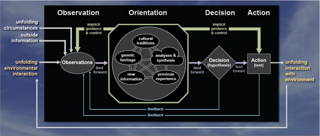
                                        IMPLICIT GUIDANCE AND CONTROL

    
    

       the final mission in real time within the structure Hardware in the Loop, where all phases of the mission are simulated and validated before the flight.

     
       
                There are 13 launch platforms qualified with our APKWS guidance section


        

                               Intelligent control                             

Intelligent control is a class of control techniques that use various artificial intelligence computing approaches like neural networks, Bayesian probability, fuzzy logic, machine learning, reinforcement learning, evolutionary computation and genetic algorithms . 

Intelligent control can be divided into the following major sub-domains:

• Neural network control
• Machine learning control
• Reinforcement learning
• Bayesian control
• Fuzzy control
• Neuro-fuzzy control
• Expert Systems
• Genetic control

New control techniques are created continuously as new models of intelligent behavior are created and computational methods developed to support them.

Neural network controllers

Neural networks have been used to solve problems in almost all spheres of science and technology. Neural network control basically involves two steps:

• System identification
• Control

It has been shown that a feedforward network with nonlinear, continuous and differentiable activation functions have universal approximation capability. Recurrent networks have also been used for system identification. Given, a set of input-output data pairs, system identification aims to form a mapping among these data pairs. Such a network is supposed to capture the dynamics of a system. For the control part, deep reinforcement learning has shown its ability to control complex systems.

Bayesian controllers

Bayesian probability has produced a number of algorithms that are in common use in many advanced control systems, serving as state space estimators of some variables that are used in the controller.

The Kalman filter and the Particle filter are two examples of popular Bayesian control components. The Bayesian approach to controller design often requires an important effort in deriving the so-called system model and measurement model, which are the mathematical relationships linking the state variables to the sensor measurements available in the controlled system. In this respect, it is very closely linked to the system-theoretic approach to control design.

      

           Applications of artificial intelligence          

Artificial intelligence, defined as intelligence exhibited by machines, has many applications in today's society. More specifically, it is Weak AI, the form of AI where programs are developed to perform specific tasks, that is being utilized for a wide range of activities including medical diagnosis, electronic trading platforms, robot control, and remote sensing. AI has been used to develop and advance numerous fields and industries, including finance, healthcare, education, transportation, and more.

The Air Operations Division (AOD) uses AI for the rule based expert systems. The AOD has use for artificial intelligence for surrogate operators for combat and training simulators, mission management aids, support systems for tactical decision making, and post processing of the simulator data into symbolic summaries.

The use of artificial intelligence in simulators is proving to be very useful for the AOD. Airplane simulators are using artificial intelligence in order to process the data taken from simulated flights. Other than simulated flying, there is also simulated aircraft warfare. The computers are able to come up with the best success scenarios in these situations. The computers can also create strategies based on the placement, size, speed and strength of the forces and counter forces. Pilots may be given assistance in the air during combat by computers. The artificial intelligent programs can sort the information and provide the pilot with the best possible maneuvers, not to mention getting rid of certain maneuvers that would be impossible for a human being to perform. Multiple aircraft are needed to get good approximations for some calculations so computer simulated pilots are used to gather data.^[6] These computer simulated pilots are also used to train future air traffic controllers.

The system used by the AOD in order to measure performance was the Interactive Fault Diagnosis and Isolation System, or IFDIS. It is a rule based expert system put together by collecting information from TF-30 documents and the expert advice from mechanics that work on the TF-30. This system was designed to be used for the development of the TF-30 for the RAAF F-111C. The performance system was also used to replace specialized workers. The system allowed the regular workers to communicate with the system and avoid mistakes, miscalculations, or having to speak to one of the specialized workers.

The AOD also uses artificial intelligence in speech recognition software. The air traffic controllers are giving directions to the artificial pilots and the AOD wants to the pilots to respond to the ATC's with simple responses. The programs that incorporate the speech software must be trained, which means they use neural networks. The program used, the Verbex 7000, is still a very early program that has plenty of room for improvement. The improvements are imperative because ATCs use very specific dialog and the software needs to be able to communicate correctly and promptly every time.

The Artificial Intelligence supported Design of Aircraft,^[7] or AIDA, is used to help designers in the process of creating conceptual designs of aircraft. This program allows the designers to focus more on the design itself and less on the design process. The software also allows the user to focus less on the software tools. The AIDA uses rule based systems to compute its data. This is a diagram of the arrangement of the AIDA modules. Although simple, the program is proving effective.

In 2003, NASA's Dryden Flight Research Center, and many other companies, created software that could enable a damaged aircraft to continue flight until a safe landing zone can be reached.^[8] The software compensates for all the damaged components by relying on the undamaged components. The neural network used in the software proved to be effective and marked a triumph for artificial intelligence.

The Integrated Vehicle Health Management system, also used by NASA, on board an aircraft must process and interpret data taken from the various sensors on the aircraft. The system needs to be able to determine the structural integrity of the aircraft. The system also needs to implement protocols in case of any damage taken the vehicle.^[9]

Haitham Baomar and Peter Bentley are leading a team from the University College of London to develop an artificial intelligence based Intelligent Autopilot System (IAS) designed to teach an autopilot system to behave like a highly experienced pilot who is faced with an emergency situation such as severe weather, turbulence, or system failure.^[10] Educating the autopilot relies on the concept of supervised machine learning “which treats the young autopilot as a human apprentice going to a flying school”. The autopilot records the actions of the human pilot generating learning models using artificial neural networks. The autopilot is then given full control and observed by the pilot as it executes the training exercise.

The Intelligent Autopilot System combines the principles of Apprenticeship Learning and Behavioural Cloning whereby the autopilot observes the low-level actions required to maneuver the airplane and high-level strategy used to apply those actions.IAS implementation employs three phases; pilot data collection, training, and autonomous control. Baomar and Bentley’s goal is to create a more autonomous autopilot to assist pilots in responding to emergency situations.

Computer science

AI researchers have created many tools to solve the most difficult problems in computer science. Many of their inventions have been adopted by mainstream computer science and are no longer considered a part of AI. (See AI effect.) According to Russell & Norvig (2003, p. 15), all of the following were originally developed in AI laboratories: time sharing,interactive interpreters, graphical user interfaces and the computer mouse, Rapid application development environments, the linked list data structure, automatic storage management, symbolic programming, functional programming, dynamic programming and object-oriented programming.

AI can be used to potentially determine the developer of anonymous binaries.

AI can be used to create other AI. For example, around November 2017, Google's AutoML project to evolve new neural net topologies created NASNet, a system optimized for ImageNet and COCO. According to Google, NASNet's performance exceeded all previously published ImageNet performance .

Power electronics

Power electronics converters are an enabling technology for renewable energy, energy storage, electric vehicles and high-voltage direct current transmission systems within the electrical grid. These converters are prone to failures and such failures can cause down times that may require costly maintenance or even have catastrophic consequences in mission critical applications. Researchers are using AI to do the automated design process for reliable power electronics converters, by calculating exact design parameters that ensure desired lifetime of the converter under specified mission profile

 
                                                            



________________________________________________________________________________