

A network address is an identifier for a node or host on a telecommunications network. Network addresses are designed to be unique identifiers across the network, although some networks allow for local, private addresses or locally administered addresses that may not be globally unique. Special network addresses are allocated as broadcast or multicast addresses. These too are not globally unique.
In some cases, network hosts may have more than one network address; for example, each network interface may be uniquely identified. Further, because protocols are frequently layered, more than one protocol's network address can occur in any particular network interface or node and more than one type of network address may be used in any one network.
Examples of network addresses include:
- Telephone number, in the public switched telephone network
- IP address in IP networks including the Internet
- IPX address, in NetWare
- X.25 or X.21 address, in a circuit switched data network
- MAC address, in Ethernet and other related network technologies
Network Address
A network address is any logical or physical address that uniquely distinguishes a network node or device over a computer or telecommunications network. It is a numeric/symbolic number or address that is assigned to any device that seeks access to or is part of a network .
A network address is a key networking technology component that facilitates identifying a network node/device and reaching a device over a network. It has several forms, including the Internet Protocol (IP) address, media access control (MAC) address and host address. It Computers on a network use a network address to identify, locate and address other computers. Besides individual devices, a network address is typically unique for each interface; for example, a computer's Wi-Fi and local area network (LAN) card has separate network addresses.
A network address is also known as the numerical network part of an
IP address. This is used to distinguish a network that has its own hosts
and addresses. For example, in the IP address 192.168.1.0, the network
address is 192.168.1.
Addresses and Names
Ethernet Addresses and Names
The basic concept of Ethernet networking is
that packets are given destination addresses by senders, and those
addresses are read and recognized by the appropriate receivers. Devices
on the network check every packet, but fully process only those packets
addressed either to themselves or to some group to which the device
belongs.
Omnipeek recognizes three types of
addresses: physical addresses, logical addresses, and symbolic names
assigned to either of these.
Physical addresses
A physical address is the hardware-level
address used by the Ethernet interface to communicate on the network.
Every device must have a unique physical address. This is often referred
to as its MAC (Media Access Control) address. An Ethernet physical
address is six bytes long and consists of six hexadecimal numbers,
usually separated by colon characters (:). For example:
Typically, a hardware manufacturer obtains a
block of physical address numbers from the IEEE and assigns a unique
physical address to each card it builds. The vendor block of addresses
is designated by the first three bytes of the six-byte physical Ethernet
address. In this way, Ethernet physical addresses are generally
distinct from each other, although some networks and protocols will
override this built-in mechanism with one of their own.
The following figure shows captured packets that use physical addresses to represent the source and destination:
Logical addresses
A logical address is a network-layer address
that is interpreted by a protocol handler. Logical addresses are used
by networking software to allow packets to be independent of the
physical connection of the network, that is, to work with different
network topologies and types of media. Each type of protocol has a
different kind of logical address, for example:
-
- an IP address (IPv4) consists of four decimal numbers separated by period (.) characters, for example:
130.57.64.11
- an IP address (IPv4) consists of four decimal numbers separated by period (.) characters, for example:
- an AppleTalk address consists of two decimal numbers separated by a period (.), for example:
2010.42
368.12
Depending on the type of protocol in a
packet (such as IP or AppleTalk), a packet may also specify source and
destination logical address information, either as extensions to the
physical addresses or as alternatives to them.
For example, in sending a packet to a
different network, the higher-level, logical destination address might
be for the computer on that network to which you are sending the packet,
while the lower-level, physical address might be the physical address
of an inter-network device, like a router, that connects the two
networks and is responsible for forwarding the packet to the ultimate
destination.
The following figure shows captured packets
identified by logical addresses under two protocols: AppleTalk (two
decimal numbers, separated by a period) and IP (four decimal numbers
from 0 to 255 separated by a period). It also shows symbolic names
substituted for IP addresses and for an AppleTalk address (Caxton).
Symbolic names
The strings of numbers typically used to
designate physical and logical addresses are perfect for machines, but
awkward for human beings to remember and use. Symbolic names stand in
for either physical or logical addresses. The domain names of the
Internet are an example of symbolic names. The relationship between the
symbolic names and the logical addresses to which they refer is handled
by DNS (Domain Name Services) in IP (Internet Protocol). Omnipeek takes
advantage of these services to allow you to resolve IP names and
addresses either passively in the background or actively for any
highlighted packets.
In addition, Omnipeek allows you to identify
devices by symbolic names of your own by creating a Name Table that
associates the names you wish to use with their corresponding addresses.
To use symbolic names that are unique to
your site, you must first create Name Table entries in Omnipeek and then
instruct Omnipeek to use names instead of addresses when names are
available.
Other classes of addresses
When one says “address,” one typically
thinks of a particular workstation or device on the network, but there
are other types of addresses equally important in networking. To send
information to everyone, you need a broadcast address. To send it to some but not all, a multicast
address is useful. If machines are to converse with more than one
partner at a time, the protocol needs to define some way of
distinguishing among services or among specific conversations. Ports and Sockets are used for these functions. Each of these is discussed in more detail below.
Broadcast and multicast addresses
It is often useful to send the same
information to more than one device, or even to all devices on a network
or group of networks. To facilitate this, the hardware and the protocol
stacks designed to run on the IEEE 802 family of networks can tell
devices to listen, not only for packets addressed to that particular
device, but also for packets whose destination is a reserved broadcast
or multicast address.
Broadcast packets are processed by every
device on the originating network segment and on any other network
segment to which the packet can be forwarded. Because broadcast packets
work in this way, most routers are set up to refuse to forward broadcast
packets. Without that provision, networks could easily be flooded by
careless broadcasting.
An alternative to broadcasting is
multicasting. Each protocol or network standard reserves certain
addresses as multicast addresses. Devices may then choose to listen in
for traffic addressed to one or more of these multicast addresses. They
capture and process only the packets addressed to the particular
multicast address(es) for which they are listening. This permits the
creation of elective groups of devices, even across network boundaries,
without adding anything to the packet processing load of machines not
interested in the multicasts. Internet routers, for example, use
multicast addresses to exchange routing information.
Hardware Broadcast Address. The following destination physical address is the Ethernet Broadcast address:
FF:FF:FF:FF:FF:FF
FF:FF:FF:FF:FF:FF
Some protocol types have logical Broadcast
addresses. When an address space is subnetted, the last (highest number)
address is typically reserved for broadcasts. For example:
IP Broadcast Addresses typically uses 255 as the host portion of the address; for example:
130.57.255.255
130.57.255.255
While conceptually very powerful, broadcast
packets can be very expensive in terms of network resources. Every
single node on the network must spend the time and memory to receive and
process a broadcast packet, even if the packet has no meaning or value
for that node.
Multicast Address.
In Ethernet, addresses in which the first byte of the address is an
odd-number are reserved for multicasting. In IPv4, all of the Class D
addresses have been reserved for multicasting purposes. That is, all the
addresses between 224.0.0.0 and 239.255.255.255 are associated with
some form of multicasting. Multicasting under AppleTalk is handled by an
AppleTalk router which associates hardware multicast addresses with
addresses in an AppleTalk Zone.
Ports and sockets
Network servers, and even workstations, need
to be able to provide a variety of services to clients and peers on the
network. To help manage these various functions, protocol designers
created the idea of logical ports to which requests for particular services could be addressed.
Ports and sockets
have slightly different meanings in some protocols. What is called a
port in TCP/UDP is essentially the same as what is called a socket in
IPX, for example. Omnipeek treats the two as equivalent. ProtoSpecs uses
port assignments and socket information to deduce the type of traffic
contained in packets.
Address space
In computing, an address space defines a range of discrete addresses, each of which may correspond to a network host, peripheral device, disk sector, a memory cell or other logical or physical entity.
For software programs to save and retrieve stored data, each unit of data must have an address where it can be individually located or else the program will be unable to find and manipulate the data. The number of address spaces available will depend on the underlying address structure and these will usually be limited by the computer architecture being used.Address spaces are created by combining enough uniquely identified qualifiers to make an address unambiguous within the address space. For a person's physical address, the address space would be a combination of locations, such as a neighborhood, town, city, or country. Some elements of an address space may be the same, but if any element in the address is different than addresses in said space will reference different entities. An example could be that there are multiple buildings at the same address of "32 Main Street" but in different towns, demonstrating that different towns have different, although similarly arranged, street address spaces.
An address space usually provides (or allows) a partitioning to several regions according to the mathematical structure it has. In the case of total order, as for memory addresses, these are simply chunks. Some nested domain hierarchies appear in the case of directed ordered tree as for the Domain Name System or a directory structure; this is similar to the hierarchical design of postal addresses. In the Internet, for example, the Internet Assigned Numbers Authority (IANA) allocates ranges of IP addresses to various registries in order to enable them to each manage their parts of the global Internet address space .
Examples
Uses of addresses include, but are not limited to the following:- Memory addresses for main memory, memory-mapped I/O, as well as for virtual memory;
- Device addresses on an expansion bus;
- Sector addressing for disk drives;
- File names on a particular volume;
- Various kinds of network host addresses in computer networks;
- Uniform resource locators in the Internet.
Address mapping and translation

Illustration of translation from logical block addressing to physical geometry
The Domain Name System maps its names to (and from) network-specific addresses (usually IP addresses), which in turn may be mapped to link layer network addresses via Address Resolution Protocol. Also, network address translation may occur on the edge of different IP spaces, such as a local area network and the Internet.

Virtual address space and physical address space relationship
namespace is a set of symbols that are used to organize objects of various kinds, so that these objects may be referred to by name. Prominent examples include:
- file systems are namespaces that assign names to files;
- some programming languages organize their variables and subroutines in namespaces;
- computer networks and distributed systems assign names to resources, such as computers, printers, websites, (remote) files, etc.
In a similar way, hierarchical file systems organize files in directories. Each directory is a separate namespace, so that the directories "letters" and "invoices" may both contain a file "to_jane".
In computer programming, namespaces are typically employed for the purpose of grouping symbols and identifiers around a particular functionality and to avoid name collisions between multiple identifiers that share the same name.
In networking, the Domain Name System organizes websites (and other resources) into hierarchical namespaces.
Name conflicts
Element names are defined by the developer. This often results in a conflict when trying to mix XML documents from different XML applications.This XML carries HTML table information:
<table>
  <tr>
    <td>Apples</td>
    <td>Oranges</td>
  </tr>
</table>
<table>
  <name>African Coffee Table</name>
  <width>80</width>
  <length>120</length>
</table>
An XML parser will not know how to handle these differences.
Solution via prefix
Name conflicts in XML can easily be avoided using a name prefix.The following XML distinguishes between information about the HTML table and furniture by prefixing "h" and "f" at the beginning xml/xml_namespaces.asp
<h:table>
  <h:tr>
    <h:td>Apples</h:td>
    <h:td>Oranges</h:td>
  </h:tr>
</h:table>

<f:table>
  <f:name>African Coffee Table</f:name>
  <f:width>80</f:width>
  <f:length>120</f:length>
</f:table>
Naming system
A name in a namespace consists of a namespace identifier and a local name. The namespace name is usually applied as a prefix to the local name.In augmented Backus–Naur form:
name = <namespace identifier> separator <local name>When local names are used by themselves, name resolution is used to decide which (if any) particular item is alluded to by some particular local name.
Examples
| Context | Name | Namespace identifier | Local name |
|---|---|---|---|
| Path | /home/user/readme.txt | /home/user (path) | readme.txt (file name) |
| Domain name | www.example.com | example.com (domain) | www (host name) |
| C++ | std::array | std | array |
| UN/LOCODE | US NYC | US (country) | NYC (locality) |
| XML | xmlns:xhtml="http://www.w3.org/1999/xhtml" <xhtml:body> |
http://www.w3.org/1999/xhtml | body |
| Perl | $DBI::errstr | DBI | $errstr |
| Java | java.util.Date | java.util | Date |
| Uniform resource name (URN) | urn:nbn:fi-fe19991055 | urn:nbn (National Bibliography Numbers) | fi-fe19991055 |
| Handle System | 10.1000/182 | 10 (Handle naming authority) | 1000/182 (Handle local name) |
| Digital object identifier | 10.1000/182 | 10.1000 (publisher) | 182 (publication) |
| MAC address | 01-23-45-67-89-ab | 01-23-45 (organizationally unique identifier) | 67-89-ab (NIC specific) |
| PCI ID | 1234 abcd | 1234 (Vendor ID) | abcd (Device ID) |
| USB VID/PID | 2341 003f | 2341 (Vendor ID) | 003f (Product ID) |
Delegation
Delegation of responsibilities between parties is important in real-world applications, such as the structure of the World Wide Web. Namespaces allow delegation of identifier assignment to multiple name issuing organisations whilst retaining global uniqueness. A central Registration authority registers the assigned namespace identifiers allocated. Each namespace identifier is allocated to an organisation which is subsequently responsible for the assignment of names in their allocated namespace. This organisation may be a name issuing organisation that assign the names themselves, or another Registration authority which further delegates parts of their namespace to different organisations.Hierarchy
A naming scheme that allows subdelegation of namespaces to third parties is a hierarchical namespace.A hierarchy is recursive if the syntax for the namespace identifiers is the same for each subdelegation. An example of a recursive hierarchy is the Domain name system.
An example of a non-recursive hierarchy are Uniform resource name representing an Internet Assigned Numbers Authority (IANA) number.
| Registry | Registrar | Example Identifier | Namespace identifier | Namespace |
|---|---|---|---|---|
| Uniform resource name (URN) | Internet Assigned Numbers Authority | urn:isbn:978-3-16-148410-0 | urn | Formal URN namespace |
| Formal URN namespace | Internet Assigned Numbers Authority | urn:isbn:978-3-16-148410-0 | ISBN | International Standard Book Numbers as Uniform Resource Names |
| International Article Number (EAN) | GS1 | 978-3-16-148410-0 | 978 | Bookland |
| International Standard Book Number (ISBN) | International ISBN Agency | 3-16-148410-X | 3 | German-speaking countries |
| German publisher code | Agentur für Buchmarktstandards | 3-16-148410-X | 16 | Mohr Siebeck |
Namespace versus scope
A namespace identifier may provide context (Scope in computer science) to a name, and the terms are sometimes used interchangeably. However, the context of a name may also be provided by other factors, such as the location where it occurs or the syntax of the name.| Without a namespace | With a namespace | |
|---|---|---|
| Local scope | Vehicle registration plate | Relative path in a File system |
| Global scope | Universally unique identifier | Domain Name System |
As a rule, names in a namespace cannot have more than one meaning; that is, different meanings cannot share the same name in the same namespace. A namespace is also called a context, because the same name in different namespaces can have different meanings, each one appropriate for its namespace.
Following are other characteristics of namespaces:
- Names in the namespace can represent objects as well as concepts, be the namespace a natural or ethnic language, a constructed language, the technical terminology of a profession, a dialect, a sociolect, or an artificial language (e.g., a programming language).
- In the Java programming language, identifiers that appear in namespaces have a short (local) name and a unique long "qualified" name for use outside the namespace.
- Some compilers (for languages such as C++) combine namespaces and names for internal use in the compiler in a process called name mangling.
#include <iostream>
// how one brings a name into the current scope
// in this case, it's bringing them into global scope
using std::cout;
using std::endl;

namespace Box1 {
   int boxSide = 4;
}

namespace Box2 {
   int boxSide = 12;
}

int main() {
  int boxSide = 42;
  cout << Box1::boxSide << endl;  //output 4
  cout << Box2::boxSide << endl;  //output 12
  cout << boxSide << endl;  // output 42
  return 0;
}
Computer-science considerations
A namespace in computer science (sometimes also called a name scope), is an abstract container or environment created to hold a logical grouping of unique identifiers or symbols (i.e. names). An identifier defined in a namespace is associated only with that namespace. The same identifier can be independently defined in multiple namespaces. That is, an identifier defined in one namespace may or may not have the same meaning as the same identifier defined in another namespace. Languages that support namespaces specify the rules that determine to which namespace an identifier (not its definition) belongs.This concept can be illustrated with an analogy. Imagine that two companies, X and Y, each assign ID numbers to their employees. X should not have two employees with the same ID number, and likewise for Y; but it is not a problem for the same ID number to be used at both companies. For example, if Bill works for company X and Jane works for company Y, then it is not a problem for each of them to be employee #123. In this analogy, the ID number is the identifier, and the company serves as the namespace. It does not cause problems for the same identifier to identify a different person in each namespace.
In large computer programs or documents it is common to have hundreds or thousands of identifiers. Namespaces (or a similar technique, see Emulating namespaces) provide a mechanism for hiding local identifiers. They provide a means of grouping logically related identifiers into corresponding namespaces, thereby making the system more modular.
Data storage devices and many modern programming languages support namespaces. Storage devices use directories (or folders) as namespaces. This allows two files with the same name to be stored on the device so long as they are stored in different directories. In some programming languages (e.g. C++, Python), the identifiers naming namespaces are themselves associated with an enclosing namespace. Thus, in these languages namespaces can nest, forming a namespace tree. At the root of this tree is the unnamed global namespace.
Use in common languages
- C++
namespace abc {
 int bar;
}
Within this block, identifiers can be used exactly as they are
declared. Outside of this block, the namespace specifier must be
prefixed. For example, outside of namespace abc, bar must be written abc::bar to be accessed. C++ includes another construct that makes this verbosity unnecessary. By adding the line
using namespace abc;to a piece of code, the prefix
abc:: is no longer needed.
Code that is not explicitly declared within a namespace is considered to be in the global namespace.
Namespace resolution in C++ is hierarchical. This means that within the hypothetical namespace
food::soup, the identifier chicken refers to food::soup::chicken. If food::soup::chicken doesn't exist, it then refers to food::chicken. If neither food::soup::chicken nor food::chicken exist, chicken refers to ::chicken, an identifier in the global namespace.
Namespaces in C++ are most often used to avoid naming collisions. Although namespaces are used extensively in recent C++ code, most older code does not use this facility because it did not exist in early versions of the language. For example, the entire C++ Standard Library is defined within
namespace std, but before standardization many components were originally in the global namespace. A programmer can insert the using
directive to bypass namespace resolution requirements and obtain
backwards compatibility with older code that expects all identifiers to
be in the global namespace. However, use of the using
directive for reasons other than backwards compatibility (e.g.,
convenience), it is considered to be against good code practices.
- Java
class String in package java.lang can be referred to as java.lang.String (this is known as the fully qualified class name). Like C++, Java offers a construct that makes it unnecessary to type the package name (import). However, certain features (such as reflection) require the programmer to use the fully qualified name.
Unlike C++, namespaces in Java are not hierarchical as far as the syntax of the language is concerned. However, packages are named in a hierarchical manner. For example, all packages beginning with
java are a part of the Java platform—the package java.lang contains classes core to the language, and java.lang.reflect contains core classes specifically relating to reflection.
In Java (and Ada, C#, and others), namespaces/packages express semantic categories of code. For example, in C#,
namespace System contains code provided by the system (the .NET Framework). How specific these categories are and how deep the hierarchies go differ from language to language.
Function and class scopes can be viewed as implicit namespaces that are inextricably linked with visibility, accessibility, and object lifetime.
- C#
System.Console.WriteLine("Hello World!");
int i = System.Convert.ToInt32("123");
or add a using statement. This, eliminates the need to mention the complete name of all classes in that namespace.
using System;
.
.
.
Console.WriteLine("Hello World!");
int i = Convert.ToInt32("123");
In the above examples, System is a namespace, and Console and Convert are classes defined within System.
- Python
# assume module a defines two functions : func1() and func2() and one class : class1
import modulea

modulea.func1()
modulea.func2()
a = modulea.class1()
The "from ... import ..." can be used to insert the relevant names directly into the calling module's namespace, and those names can be accessed from the calling module without the qualified name :
# assume modulea defines two functions : func1() and func2() and one class : class1
from modulea import func1

func1()
func2() # this will fail as an undefined name, as will the full name modulea.func2()
a = class1() # this will fail as an undefined name, as will the full name modulea.class1()
Since this directly imports names (without qualification) it can overwrite existing names with no warnings.
A special form is "from ... import *", which imports all names defined in the named package directly in the calling modules namespace. Use of this form of import, although supported within the language, is generally discouraged as it pollutes the namespace of the calling module and will cause already defined names to be overwritten in the case of name clashes.
Python also supports "import x as y" as a way of providing an alias or alternative name for use by the calling module:
import numpy as np
a = np.arange(1000)
- XML namespace
- PHP
# assume this is a class file defines two functions : foo() and bar()
# location of the file phpstar/foobar.php
namespace phpstar;
class fooBar
{
    public function foo()
    {
        echo 'hello world, from function foo';
    }

    public function bar()
    {
        echo 'hello world, from function bar';
    }
}
We can reference a PHP namespace with the following different ways:
# location of the file index.php
# Include the file
include "phpstar/foobar.php";

# Option 1: directly prefix the class name with the namespace
$obj_foobar = new \phpstar\fooBar();

# Option 2: import the namespace
use phpstar\fooBar;
$obj_foobar = new fooBar();

# Option 2a: import & alias the namespace
use phpstar\fooBar as FB;
$obj_foobar = new FB();

# Access the properties and methods with regular way
$obj_foobar->foo();
$obj_foobar->bar();
Emulating namespaces
In programming languages lacking language support for namespaces, namespaces can be emulated to some extent by using an identifier naming convention. For example, C libraries such as Libpng often use a fixed prefix for all functions and variables that are part of their exposed interface. Libpng exposes identifiers such as:png_create_write_struct png_get_signature png_read_row png_set_invalidThis naming convention provides reasonable assurance that the identifiers are unique and can therefore be used in larger programs without naming collisions. Likewise, many packages originally written in Fortran (e.g., BLAS, LAPACK) reserve the first few letters of a function's name to indicate which group it belongs to.
This technique has several drawbacks:
- It doesn't scale well to nested namespaces; identifiers become excessively long since all uses of the identifiers must be fully namespace-qualified.
- Individuals or organizations may use dramatically inconsistent naming conventions, potentially introducing unwanted obfuscation.
- Compound or "query-based" operations on groups of identifiers, based on the namespaces in which they are declared, are rendered unwieldy or unfeasible.
- In languages with restricted identifier length, the use of prefixes
limits the number of characters that can be used to identify what the
function does. This is a particular problem for packages originally
written in FORTRAN 77, which offered only 6 characters per identifier. For example, the name of the BLAS function
DGEMMfunction indicates that it operates on double-precision numbers ("D") and general matrices ("GE"), and only the last two characters show what it actually does: matrix-matrix multiplication (the "MM").
- No special software tools are required to locate names in source-code files. A simple program like grep suffices.
- There are no namespace name conflicts.
- There is no need for name-mangling, and thus no potential incompatibility problems.
Digital object identifier
A DOI aims to be "resolvable", usually to some form of access to the information object to which the DOI refers. This is achieved by binding the DOI to metadata about the object, such as a URL, indicating where the object can be found. Thus, by being actionable and interoperable, a DOI differs from identifiers such as ISBNs and ISRCs which aim only to uniquely identify their referents. The DOI system uses the indecs Content Model for representing metadata.
The DOI for a document remains fixed over the lifetime of the document, whereas its location and other metadata may change. Referring to an online document by its DOI is supposed to provide a more stable link than simply using its URL. But every time a URL changes, the publisher has to update the metadata for the DOI to link to the new URL. It is the publisher's responsibility to update the DOI database. If they fail to do so, the DOI resolves to a dead link leaving the DOI useless.
The developer and administrator of the DOI system is the International DOI Foundation (IDF), which introduced it in 2000. Organizations that meet the contractual obligations of the DOI system and are willing to pay to become a member of the system can assign DOIs. The DOI system is implemented through a federation of registration agencies coordinated by the IDF. By late April 2011 more than 50 million DOI names had been assigned by some 4,000 organizations, and by April 2013 this number had grown to 85 million DOI names assigned through 9,500 organizations.
Nomenclature and syntax
A DOI is a type of Handle System handle, which takes the form of a character string divided into two parts, a prefix and a suffix, separated by a slash.prefix/suffix
10.NNNN, where NNNN is a series of at least 4 numbers greater than or equal to 1000, whose limit depends only on the total number of registrants. The prefix may be further subdivided with periods, like 10.NNNN.N.
For example, in the DOI name
10.1000/182, the prefix is 10.1000 and the suffix is 182.
The "10." part of the prefix distinguishes the handle as part of the
DOI namespace, as opposed to some other Handle System namespace,[A] and the characters 1000 in the prefix identify the registrant; in this case the registrant is the International DOI Foundation itself. 182 is the suffix, or item ID, identifying a single object (in this case, the latest version of the DOI Handbook).
DOI names can identify creative works (such as texts, images, audio or video items, and software) in both electronic and physical forms, performances, and abstract works such as licenses, parties to a transaction, etc.
The names can refer to objects at varying levels of detail: thus DOI names can identify a journal, an individual issue of a journal, an individual article in the journal, or a single table in that article. The choice of level of detail is left to the assigner, but in the DOI system it must be declared as part of the metadata that is associated with a DOI name, using a data dictionary based on the indecs Content Model.
Display
The official DOI Handbook explicitly states that DOIs should display on screens and in print in the formatdoi:10.1000/182.
Contrary to the DOI Handbook, CrossRef, a major DOI registration agency, recommends displaying a URL (for example,
https://doi.org/10.1000/182) instead of the officially specified format (for example, doi:10.1000/182)[16][17] This URL is persistent (there is a contract that ensures persistence in the DOI.ORG domain), so it is a PURL — providing the location of an HTTP proxy server which will redirect web accesses to the correct online location of the linked item.
The CrossRef recommendation is primarily based on the assumption that the DOI is being displayed without being hyper-linked to its appropriate URL – the argument being that without the hyperlink it is not as easy to copy-and-paste the full URL to actually bring up the page for the DOI, thus the entire URL should be displayed, allowing people viewing the page containing the DOI to copy-and-paste the URL, by hand, into a new window/tab in their browser in order to go to the appropriate page for the document the DOI represents.
Applications
Major applications of the DOI system currently include:- scholarly materials (journal articles, books, ebooks,etc.) through CrossRef, a consortium of around 3,000 publishers; Airiti, a leading provider of electronic academic journals in Chinese and Taiwanese; and the Japan Link Center (JaLC) an organization providing link management and DOI assignment for electronic academic journals in Japanese.
- research datasets through DataCite, a consortium of leading research libraries, technical information providers, and scientific data centers;
- European Union official publications through the EU publications office;
- the Chinese National Knowledge Infrastructure project at Tsinghua University and the Institute of Scientific and Technical Information of China (ISTIC), two initiatives sponsored by the Chinese government.
- Permanent global identifiers for commercial video content through the Entertainment ID Registry, commonly known as EIDR.
Other registries include Crossref and the multilingual European DOI Registration Agency. Since 2015, RFCs can be referenced as
doi:10.17487/rfc….
DOI and other special identifiers can help to unify information about references with different spelling in various language versions of Wikipedia.
Features and benefits
The IDF designed the DOI system to provide a form of persistent identification, in which each DOI name permanently and unambiguously identifies the object to which it is associated. It also associates metadata with objects, allowing it to provide users with relevant pieces of information about the objects and their relationships. Included as part of this metadata are network actions that allow DOI names to be resolved to web locations where the objects they describe can be found. To achieve its goals, the DOI system combines the Handle System and the indecs Content Model with a social infrastructure.The Handle System ensures that the DOI name for an object is not based on any changeable attributes of the object such as its physical location or ownership, that the attributes of the object are encoded in its metadata rather than in its DOI name, and that no two objects are assigned the same DOI name. Because DOI names are short character strings, they are human-readable, may be copied and pasted as text, and fit into the URI specification. The DOI name-resolution mechanism acts behind the scenes, so that users communicate with it in the same way as with any other web service; it is built on open architectures, incorporates trust mechanisms, and is engineered to operate reliably and flexibly so that it can be adapted to changing demands and new applications of the DOI system. DOI name-resolution may be used with OpenURL to select the most appropriate among multiple locations for a given object, according to the location of the user making the request. However, despite this ability, the DOI system has drawn criticism from librarians for directing users to non-free copies of documents that would have been available for no additional fee from alternative locations.
The indecs Content Model as used within the DOI system associates metadata with objects. A small kernel of common metadata is shared by all DOI names and can be optionally extended with other relevant data, which may be public or restricted. Registrants may update the metadata for their DOI names at any time, such as when publication information changes or when an object moves to a different URL.
The International DOI Foundation (IDF) oversees the integration of these technologies and operation of the system through a technical and social infrastructure. The social infrastructure of a federation of independent registration agencies offering DOI services was modelled on existing successful federated deployments of identifiers such as GS1 and ISBN.
Comparison with other identifier schemes
A DOI name differs from commonly used Internet pointers to material, such as the Uniform Resource Locator (URL), in that it identifies an object itself as a first-class entity, rather than the specific place where the object is located at a certain time. It implements the Uniform Resource Identifier (Uniform Resource Name) concept and adds to it a data model and social infrastructure.A DOI name also differs from standard identifier registries such as the ISBN, ISRC, etc. The purpose of an identifier registry is to manage a given collection of identifiers, whereas the primary purpose of the DOI system is to make a collection of identifiers actionable and interoperable, where that collection can include identifiers from many other controlled collections.
The DOI system offers persistent, semantically-interoperable resolution to related current data and is best suited to material that will be used in services outside the direct control of the issuing assigner (e.g., public citation or managing content of value). It uses a managed registry (providing social and technical infrastructure). It does not assume any specific business model for the provision of identifiers or services and enables other existing services to link to it in defined ways. Several approaches for making identifiers persistent have been proposed. The comparison of persistent identifier approaches is difficult because they are not all doing the same thing. Imprecisely referring to a set of schemes as "identifiers" doesn't mean that they can be compared easily. Other "identifier systems" may be enabling technologies with low barriers to entry, providing an easy to use labeling mechanism that allows anyone to set up a new instance (examples include Persistent Uniform Resource Locator (PURL), URLs, Globally Unique Identifiers (GUIDs), etc.), but may lack some of the functionality of a registry-controlled scheme and will usually lack accompanying metadata in a controlled scheme. The DOI system does not have this approach and should not be compared directly to such identifier schemes. Various applications using such enabling technologies with added features have been devised that meet some of the features offered by the DOI system for specific sectors (e.g., ARK).
A DOI name does not depend on the object's location and, in this way, is similar to a Uniform Resource Name (URN) or PURL but differs from an ordinary URL. URLs are often used as substitute identifiers for documents on the Internet although the same document at two different locations has two URLs. By contrast, persistent identifiers such as DOI names identify objects as first class entities: two instances of the same object would have the same DOI name.
Resolution
DOI name resolution is provided through the Handle System, developed by Corporation for National Research Initiatives, and is freely available to any user encountering a DOI name. Resolution redirects the user from a DOI name to one or more pieces of typed data: URLs representing instances of the object, services such as e-mail, or one or more items of metadata. To the Handle System, a DOI name is a handle, and so has a set of values assigned to it and may be thought of as a record that consists of a group of fields. Each handle value must have a data type specified in its<type> field, which
defines the syntax and semantics of its data. While a DOI persistently
and uniquely identifies the object to which it is assigned, DOI
resolution may not be persistent, due to technical and administrative
issues.
To resolve a DOI name, it may be input to a DOI resolver, such as doi.org.
Another approach, which avoids typing or cutting-and-pasting into a resolver is to include the DOI in a document as a URL which uses the resolver as an HTTP proxy, such as
https://doi.org/ (preferred) or http://dx.doi.org/, both of which support HTTPS. For example, the DOI 10.1000/182 can be included in a reference or hyperlink as https://doi.org/10.1000/182. This approach allows users to click on the DOI as a normal hyperlink.
Indeed, as previously mentioned, this is how CrossRef recommends that
DOIs always be represented (preferring HTTPS over HTTP), so that if they
are cut-and-pasted into other documents, emails, etc., they will be
actionable.
Other DOI resolvers and HTTP Proxies include http://hdl.handle.net, and https://doi.pangaea.de/. At the beginning of the year 2016, a new class of alternative DOI resolvers was started by http://doai.io. This service is unusual in that it tries to find a non-paywalled version of a title and redirects you to that instead of the publisher's version. Since then, other open-access favoring DOI resolvers have been created, notably https://oadoi.org/ in October 2016. While traditional DOI resolvers solely rely on the Handle System, alternative DOI resolvers first consult open access resources such as BASE (Bielefeld Academic Search Engine).
An alternative to HTTP proxies is to use one of a number of add-ons and plug-ins for browsers, thereby avoiding the conversion of the DOIs to URLs, which depend on domain names and may be subject to change, while still allowing the DOI to be treated as a normal hyperlink. For example. the CNRI Handle Extension for Firefox , enables the browser to access Handle System handles or DOIs like
hdl:4263537/4000 or doi:10.1000/1 directly in the Firefox
browser, using the native Handle System protocol. This plug-in can also
replace references to web-to-handle proxy servers with native
resolution. A disadvantage of this approach for publishers is that, at
least at present, most users will be encountering the DOIs in a browser,
mail reader, or other software which does not have one of these plug-ins installed.
IDF organizational structure
The International DOI Foundation (IDF), a non-profit organisation created in 1998, is the governance body of the DOI system. It safeguards all intellectual property rights relating to the DOI system, manages common operational features, and supports the development and promotion of the DOI system. The IDF ensures that any improvements made to the DOI system (including creation, maintenance, registration, resolution and policymaking of DOI names) are available to any DOI registrant. It also prevents third parties from imposing additional licensing requirements beyond those of the IDF on users of the DOI system.The IDF is controlled by a Board elected by the members of the Foundation, with an appointed Managing Agent who is responsible for co-ordinating and planning its activities. Membership is open to all organizations with an interest in electronic publishing and related enabling technologies. The IDF holds annual open meetings on the topics of DOI and related issues.
Registration agencies, appointed by the IDF, provide services to DOI registrants: they allocate DOI prefixes, register DOI names, and provide the necessary infrastructure to allow registrants to declare and maintain metadata and state data. Registration agencies are also expected to actively promote the widespread adoption of the DOI system, to cooperate with the IDF in the development of the DOI system as a whole, and to provide services on behalf of their specific user community. A list of current RAs is maintained by the International DOI Foundation. The IDF is recognized as one of the federated registrars for the Handle System by the DONA Foundation (of which the IDF is a board member), and is responsible for assigning Handle System prefixes under the top-level
10 prefix.
Registration agencies generally charge a fee to assign a new DOI name; parts of these fees are used to support the IDF. The DOI system overall, through the IDF, operates on a not-for-profit cost recovery basis.
Standardization
The DOI system is an international standard developed by the International Organization for Standardization in its technical committee on identification and description, TC46/SC9. The Draft International Standard ISO/DIS 26324, Information and documentation – Digital Object Identifier System met the ISO requirements for approval. The relevant ISO Working Group later submitted an edited version to ISO for distribution as an FDIS (Final Draft International Standard) ballot, which was approved by 100% of those voting in a ballot closing on 15 November 2010. The final standard was published on 23 April 2012.DOI is a registered URI under the info URI scheme specified by IETF RFC 4452. info:doi/ is the infoURI Namespace of Digital Object Identifiers.
The DOI syntax is a NISO standard, first standardised in 2000, ANSI/NISO Z39.84-2005 Syntax for the Digital Object Identifier.
The maintainers of the DOI system have deliberately not registered a DOI namespace for URNs, stating that:
URN architecture assumes a DNS-based Resolution Discovery Service (RDS) to find the service appropriate to the given URN scheme. However no such widely deployed RDS schemes currently exist.... DOI is not registered as a URN namespace, despite fulfilling all the functional requirements, since URN registration appears to offer no advantage to the DOI System. It requires an additional layer of administration for defining DOI as a URN namespace (the stringurn:doi:10.1000/1rather than the simplerdoi:10.1000/1) and an additional step of unnecessary redirection to access the resolution service, already achieved through either http proxy or native resolution. If RDS mechanisms supporting URN specifications become widely available, DOI will be registered as a URN.
— International DOI Foundation, Factsheet: DOI System and Internet Identifier Specifications
Digital identify
digital identity is information on an entity used by computer systems
to represent an external agent. That agent may be a person,
organization, application, or device. ISO/IEC 24760-1 defines identity
as "set of attributes related to an entity".
The information contained in a digital identity allows for
assessment and authentication of a user interacting with a business
system on the web, without the involvement of human operators. Digital
identities allow our access to computers and the services they provide
to be automated, and make it possible for computers to mediate
relationships.
The term "digital identity" has also come to denote aspects of civil and personal identity that have resulted from the widespread use of identity information to represent people in computer systems.
Digital identity is now often used in ways that require data about persons stored in computer systems to be linked to their civil, or national, identities. Furthermore, the use of digital identities is now so widespread that many discussions refer to "digital identity" as the entire collection of information generated by a person’s online activity. This includes usernames and passwords, online search activities, birth date, social security, and purchasing history. Especially where that information is publicly available and not anonymized, and can be used by others to discover that person's civil identity. In this wider sense, a digital identity is a version, or facet, of a person's social identity. This may also be referred to as an online identity.
The legal and social effects of digital identity are complex and challenging. However, they are simply a consequence of the increasing use of computers, and the need to provide computers with information that can be used to identify external agents.
Background
A critical problem in cyberspace is knowing with whom one is interacting. Using static identifiers such as password and email there are no ways to precisely determine the identity of a person in digital space, because this information can be stolen or used by many individuals acting as one. Digital identity based on dynamic entity relationships captured from behavioral history across multiple websites and mobile apps can verify and authenticate an identity with up to 95 percent accuracy.By comparing a set of entity relationships between a new event (e.g., login) and past events, a pattern of convergence can verify or authenticate the identity as legitimate where divergence indicates an attempt to mask an identity. Data used for digital identity is generally anonymized using a one-way hash, thereby avoiding privacy concerns. Because it is based on behavioral history, a digital identity is impossible to fake or steal.
Related terms
Subject and entity
A digital identity may also be referred to as a Digital Subject or Digital entity and is the digital representation of a set of claims made by one party about itself or another person, group, thing or concept.Attributes, preferences and traits
Every digital identity has zero or more identity attributes. Attributes are acquired and contain information about a subject, such as medical history, purchasing behaviour, bank balance, age and so on. Preferences retain a subject's choices such as favourite brand of shoes, preferred currency. Traits are features of the subject that are inherent, such as eye colour, nationality, place of birth. While attributes of a subject can change easily, traits change slowly, if at all. Digital identity also has entity relationships derived from the devices, environment and locations from which an individual transacts on the web.Technical aspects
Trust, authentication and authorization
In order to assign a digital representation to an entity, the attributing party must trust that the claim of an attribute (such as name, location, role as an employee, or age) is correct and associated with the person or thing presenting the attribute (see Authentication below). Conversely, the individual claiming an attribute may only grant selective access to its information, e.g. (proving identity in a bar or PayPal authentication for payment at a web site). In this way, digital identity is better understood as a particular viewpoint within a mutually-agreed relationship than as an objective property.Authentication
Authentication is a key aspect of trust-based identity attribution, providing a codified assurance of the identity of one entity to another. Authentication methodologies include the presentation of a unique object such as a bank credit card, the provision of confidential information such as a password or the answer to a pre-arranged question, the confirmation of ownership of an e-mail address, and more robust but relatively costly solutions utilizing encryption methodologies. In general, business-to-business authentication prioritises security while user to business authentication tends towards simplicity. Physical authentication techniques such as iris scanning, handprinting, and voiceprinting are currently being developed and in the hope of providing improved protection against identity theft. Those techniques fall into the area of Biometry (biometrics). A combination of static identifiers (Username&passwords) along with personal unique attributes (biometrics), would allow for multi factor authentication. This process would yield more creditable authentication, which in nature is much more difficult to be cracked and manipulated.Whilst technological progress in authentication continues to evolve, these systems do not prevent aliases being used. The introduction of strong authentication for online payment transactions within the European Union now links a verified person to an account, where such person has been identified in accordance with statutory requirements prior to account being opened. Verifying a person opening an account online typically requires a form of device binding to the credentials being used. This verifies that the device that stands in for a person on the Web is actually the individuals device and not the device of someone simply claiming to be the individual. The concept of reliance authentication makes use of pre-existing accounts, to piggy back further services upon those accounts, providing that the original source is reliable. The concept of reliability comes from various anti-money laundering and counter-terrorism funding legislation in the USA, EU28, Australia, Singapore and New Zealand where second parties may place reliance on the customer due diligence process of the first party, where the first party is say a financial institution. An example of reliance authentication is PayPal's verification method.
Authorization
Authorization is the determination of any entity that controls resources that the authenticated can access those resources. Authorization depends on authentication, because authorization requires that the critical attribute (i.e., the attribute that determines the authorizer's decision) must be verified. For example, authorization on a credit card gives access to the resources owned by Amazon, e.g., Amazon sends one a product. Authorization of an employee will provide that employee with access to network resources, such as printers, files, or software. For example, a database management system might be designed so as to provide certain specified individuals with the ability to retrieve information from a database but not the ability to change data stored in the database, while giving other individuals the ability to change data.[citation needed]Consider the person who rents a car and checks into a hotel with a credit card. The car rental and hotel company may request authentication that there is credit enough for an accident, or profligate spending on room service. Thus a card may be refused when trying to book the balloon trip, though there is adequate credit to pay for the rental, the hotel, and the balloon trip. Then when the person leaves the hotel and returns the car, the actual charges are authorized (too late for the balloon trip).
Valid online authorization requires analysis of information related to the digital event including device and environmental variables. These are generally derived from the hundreds of entities exchanged between a device and business server to support an event using standard Internet protocols.
Digital identifiers
Digital identity fundamentally requires digital identifiers—strings or tokens that are unique within a given scope (globally or locally within a specific domain, community, directory, application, etc.). Identifiers are the key used by the parties to an identification relationship to agree on the entity being represented. Identifiers may be classified as omnidirectional and unidirectional. Omnidirectional identifiers are intended to be public and easily discoverable, while unidirectional identifiers are intended to be private and used only in the context of a specific identity relationship.Identifiers may also be classified as resolvable or non-resolvable. Resolvable identifiers, such as a domain name or e-mail address, may be dereferenced into the entity they represent, or some current state data providing relevant attributes of that entity. Non-resolvable identifiers, such as a person's real-world name, or a subject or topic name, can be compared for equivalence but are not otherwise machine-understandable.
There are many different schemes and formats for digital identifiers. The most widely used is Uniform Resource Identifier (URI) and its internationalized version Internationalized Resource Identifier (IRI)—the standard for identifiers on the World Wide Web. OpenID and Light-Weight Identity (LID) are two web authentication protocols that use standard HTTP URIs (often called URLs), for example.
Digital Object Architecture
Digital Object Architecture (DOA) provides a means of managing digital information in a network environment. A digital object has a machine and platform independent structure that allows it to be identified, accessed and protected, as appropriate. A digital object may incorporate not only informational elements, i.e., a digitized version of a paper, movie or sound recording, but also the unique identifier of the digital object and other metadata about the digital object. The metadata may include restrictions on access to digital objects, notices of ownership, and identifiers for licensing agreements, if appropriate.Handle System
The Handle System is a general purpose distributed information system that provides efficient, extensible, and secure identifier and resolution services for use on networks such as the internet. It includes an open set of protocols, a namespace, and a reference implementation of the protocols. The protocols enable a distributed computer system to store identifiers, known as handles, of arbitrary resources and resolve those handles into the information necessary to locate, access, contact, authenticate, or otherwise make use of the resources. This information can be changed as needed to reflect the current state of the identified resource without changing its identifier, thus allowing the name of the item to persist over changes of location and other related state information. The original version of the Handle System technology was developed with support from the Defense Advanced Research Projects Agency (DARPA).Extensible Resource Identifiers
A new OASIS standard for abstract, structured identifiers, XRI (Extensible Resource Identifiers), adds new features to URIs and IRIs that are especially useful for digital identity systems. OpenID also supports XRIs, and XRIs are the basis for i-names.Risk-Based Authentication
Risk-Based Authentication is a commercial application of digital identity whereby multiple entity relationship from the device (e.g., operating system), environment (e.g., DNS Server) and data entered by a user for any given transaction is evaluated for correlation with events from known behaviors for the same identity. Analysis are performed based on quantifiable metrics, such as transaction velocity, locale settings (or attempts to obfuscate), and user-input data (such as ship-to address). Correlation and deviation are mapped to tolerances and scored, then aggregated across multiple entities to compute a transaction risk-score, which assess the risk posed to an organization.Policy aspects
There are proponents of treating self-determination and freedom of expression of digital identity as a new human right. Some have speculated that digital identities could become a new form of legal entity.Taxonomies of identity
Digital identity attributes—or data—exist within the context of ontologies.The development of digital identity network solutions that can interoperate taxonomically-diverse representations of digital identity is a contemporary challenge. Free-tagging has emerged recently as an effective way of circumventing this challenge (to date, primarily with application to the identity of digital entities such as bookmarks and photos) by effectively flattening identity attributes into a single, unstructured layer. However, the organic integration of the benefits of both structured and fluid approaches to identity attribute management remains elusive.
Networked identity
Identity relationships within a digital network may include multiple identity entities. However, in a decentralised network like the Internet, such extended identity relationships effectively require both (a) the existence of independent trust relationships between each pair of entities in the relationship and (b) a means of reliably integrating the paired relationships into larger relational units. And if identity relationships are to reach beyond the context of a single, federated ontology of identity (see Taxonomies of identity above), identity attributes must somehow be matched across diverse ontologies. The development of network approaches that can embody such integrated "compound" trust relationships is currently a topic of much debate in the blogosphere.Integrated compound trust relationships allow, for example, entity A to accept an assertion or claim about entity B by entity C. C thus vouches for an aspect of B's identity to A.
A key feature of "compound" trust relationships is the possibility of selective disclosure from one entity to another of locally relevant information. As an illustration of the potential application of selective disclosure, let us suppose a certain Diana wished to book a hire car without disclosing irrelevant personal information (utilising a notional digital identity network that supports compound trust relationships). As an adult, UK resident with a current driving license, Diana might have the UK's Driver and Vehicle Licensing Agency vouch for her driving qualification, age and nationality to a car-rental company without having her name or contact details disclosed. Similarly, Diana's bank might assert just her banking details to the rental company. Selective disclosure allows for appropriate privacy of information within a network of identity relationships.
A classic form of networked digital identity based on international standards is the "White Pages".
An electronic white pages links various devices, like computers and telephones, to an individual or organization. Various attributes such as X.509v3 digital certificates for secure cryptographic communications are captured under a schema, and published in an LDAP or X.500 directory. Changes to the LDAP standard are managed by working groups in the IETF, and changes in X.500 are managed by the ISO. The ITU did significant analysis of gaps in digital identity interoperability via the FGidm, focus group on identity management.
Implementations of X.500[2005] and LDAPv3 have occurred worldwide but are primarily located in major data centers with administrative policy boundaries regarding sharing of personal information. Since combined X.500 [2005] and LDAPv3 directories can hold millions of unique objects for rapid access, it is expected to play a continued role for large scale secure identity access services. LDAPv3 can act as a lightweight standalone server, or in the original design as a TCP-IP based Lightweight Directory Access Protocol compatible with making queries to a X.500 mesh of servers which can run the native OSI protocol.
This will be done by scaling individual servers into larger groupings that represent defined "administrative domains", (such as the country level digital object) which can add value not present in the original "White Pages" that was used to look up phone numbers and email addresses, largely now available through non-authoritative search engines.
The ability to leverage and extend a networked digital identity is made more practicable by the expression of the level of trust associated with the given identity through a common Identity Assurance Framework.
Self-sovereign identity
Self-sovereign identity (SSI) is the concept that people can store information about their digital identity in a location of their choice. This information can then provide to third parties on request. With the development of blockchain technologies decentralized identities can be based on SSI that are not owned by a single provider.e- Key Shifting issues and privacy
With automated face recognition, tagging, location tracking and widespread digital authentication systems many actions of a person become easily associated with identity, as a cause, sometimes privacy is lost and security is subverted. An identity system that builds on confirmed pseudonyms can provide privacy and enhance e- Key Shifting for digital services and transactions. Cyberspace creates opportunities for identity theft. Exact copies of everything sent over a digital communications channel can be recorded. Thus, cyberspace needs a system that allows individuals to verify their identities to others without revealing to them the digital representation of their identities.Anonymous attribute systems
An anonymous attribute is one that retains its uniqueness, but is put through a one-way hash so that it is represented in a string of characters that have no innate meaning or value. The one-way hash is an algorithm of inordinate complexity that generates the character string so that it is indecipherable compared to the original. In this way, a social security number, can be retained for attribute comparison, but the values used for comparison, while unique, would in no way resemble the original social security number.Legal issues
Clare Sullivan presents the grounds for digital identity as an emerging legal concept. The UK's Identity Cards Act 2006 confirms Sullivan's argument and unfolds the new legal concept involving database identity and transaction identity. Database identity refers to the collection of data that is registered about an individual within the databases of the scheme and transaction identity is a set of information that defines the individual's identity for transactional purposes. Although there is reliance on the verification of identity, none of the processes used are entirely trustworthy. The consequences of digital identity abuse and fraud are potentially serious, since in possible implications the person is held legally responsible.Business aspects
Corporations have begun to recognize the Internet's potential to facilitate the tailoring of the online storefront to each individual customer. Purchase suggestions, personalised adverts and other tailored marketing strategies are a great success to businesses. Such tailoring however, depends on the ability to connect attributes and preferences to the identity of the visitor.Variance by jurisdiction
While many facets of digital identity are universal owing in part to the ubiquity of the Internet, some regional variations exist due to specific laws, practices and government services that are in place. For example, Digital identity in Australia can utilize services that validate Driving licences, Passports and other physical documents online to help improve the quality of a digital identity, also strict Anti-money laundering policies mean that some services, such as money transfers need a stricter level of validation of digital identity.Base address
In computing, a base address is an address serving as a reference point ("base") for other addresses. Related addresses can be accessed using an addressing scheme.Under the relative addressing scheme, to obtain an absolute address, the relevant base address is taken and offset (aka displacement) is added to it. Under this type of scheme, the base address is the lowest numbered address within a prescribed range, to facilitate adding related positive-valued offsets.
An index register in a computer's CPU is a processor register used for modifying operand addresses during the run of a program, typically for doing vector/array operations.
The contents of an index register is added to (in some cases subtracted from) an immediate address (one that is part of the instruction itself) to form the "effective" address of the actual data (operand). Special instructions are typically provided to test the index register and, if the test fails, increments the index register by an immediate constant and branches, typically to the start of the loop. Some instruction sets allow more than one index register to be used; in that case additional instruction fields specify which index registers to use. While normally processors that allow an instruction to specify multiple index registers add the contents together, IBM had a line of computers in which the contents were or'd together.
In early computers without any form of indirect addressing, array operations had to be performed by modifying the instruction address, which required several additional program steps and used up more computer memory, a scarce resource in computer installations of the early era (as well as in early microcomputers two decades later).

Index register display on an IBM 7094 mainframe from the early 1960s.
Flash Combat
Index registers, commonly known as a B-line in early British computers, were first used in the British Manchester Mark 1 computer, in 1949. In general, index registers became a standard part of computers during the technology's second generation, roughly 1954–1966. Most[NB 1] machines in the IBM 700/7000 mainframe series had them, starting with the IBM 704 in 1954, though they were optional on some smaller machines such as the IBM 650 and IBM 1401.Early "small machines" with index registers include the AN/USQ-17, around 1960, and the 9 series of real-time computers from Scientific Data Systems, from the early 1960s.
While the Intel 8080 allowed indirect addressing via a register, the first microprocessor with a true index register appears to have been the Motorola 6800, and the similar MOS Technology 6502 made good use of two such registers.
Modern computer designs generally do not include dedicated index registers; instead they allow any general purpose register to contain an address, and allow a constant value and, on some machines, the contents of another register to be added to it as an offset to form the effective address. Early computers designed this way include the PDP-6 and the IBM System/360.
Example
Here is a simple example of index register use in assembly language pseudo-code that sums a 100 entry array of 4-byte words:Clear_accumulator Load_index 400,index2 //load 4*array size into index register 2 (index2) loop_start : Add_word_to_accumulator array_start,index2 //Add to AC the word at the address (array_start + index2) Branch_and_decrement_if_index_not_zero loop_start,4,index2 //loop decrementing by 4 until index register is zero
For loop
In computer science, a for-loop (or simply for loop) is a control flow statement for specifying iteration, which allows code to be executed repeatedly. Various keywords are used to specify this statement: descendants of ALGOL use "for", while descendants of Fortran use "do". There are other possibilities, for example COBOL which uses "PERFORM VARYING".A for-loop has two parts: a header specifying the iteration, and a body which is executed once per iteration. The header often declares an explicit loop counter or loop variable, which allows the body to know which iteration is being executed. For-loops are typically used when the number of iterations is known before entering the loop. For-loops can be thought of as shorthands for while-loops which increment and test a loop variable.
The name for-loop comes from the English word for, which is used as the keyword in many programming languages to introduce a for-loop. The term in English dates to ALGOL 58 and was popularized in the influential later ALGOL 60; it is the direct translation of the earlier German für, used in Superplan (1949–1951) by Heinz Rutishauser, who also was involved in defining ALGOL 58 and ALGOL 60. The loop body is executed "for" the given values of the loop variable, though this is more explicit in the ALGOL version of the statement, in which a list of possible values and/or increments can be specified.
In FORTRAN and PL/I, the keyword DO is used for the same thing and it is called a do-loop; this is different from a do-while loop.
for

For loop illustration, from i=0 to i=2, resulting in data1=200
Traditional for-loops
The for-loop of languages like ALGOL, Simula, BASIC, Pascal, Modula, Oberon, Ada, Matlab, Ocaml, F#, and so on, requires a control variable with start- and end-values and looks something like this:for i = first to last do statement
(* or just *)
for i = first..last do statement
int
even in the numerical case). An optional step-value (an increment or
decrement ≠ 1) may also be included, although the exact syntaxes used
for this differs a bit more between the languages. Some languages
require a separate declaration of the control variable, some do not.
Another form was popularized by the C programming language. It requires 3 parts: the initialization, the condition, and the afterthought and all these three parts are optional.
The initialization declares (and perhaps assigns to) any variables required. The type of a variable should be same if you are using multiple variables in initialization part. The condition checks a condition, and quits the loop if false. The afterthought is performed exactly once every time the loop ends and then repeats.
Here is an example of the traditional for-loop in Java.
// Prints the numbers 0 to 99 (and not 100), each followed by a space.
for (int i=0; i<100; i++)
{
    System.out.print(i);
    System.out.print(' ');
}
System.out.println();
Iterator-based for-loops
This type of for-loop is a generalisation of the numeric range type of for-loop, as it allows for the enumeration of sets of items other than number sequences. It is usually characterized by the use of an implicit or explicit iterator, in which the loop variable takes on each of the values in a sequence or other data collection. A representative example in Python is:for item in some_iterable_object:
do_something()
do_something_else()
some_iterable_object is either a data collection
that supports implicit iteration (like a list of employee's names), or
may in fact be an iterator itself. Some languages have this in addition
to another for-loop syntax; notably, PHP has this type of loop under the
name for each, as well as a three-expression for-loop (see below) under the name for.
Vectorised for-loops
Some languages offer a for-loop that acts as if processing all iterations in parallel, such as thefor all keyword in FORTRAN 95 which has the interpretation that all right-hand-side expressions are evaluated before any assignments are made, as distinct from the explicit iteration form. For example, in the for statement in the following pseudocode fragment, when calculating the new value for A(i), except for the first (with i = 2) the reference to A(i - 1) will obtain the new value that had been placed there in the previous step. In the for all version, however, each calculation refers only to the original, unaltered A.
for     i := 2 : N - 1 do A(i) := [A(i - 1) + A(i) + A(i + 1)] / 3; next i;
for all i := 2 : N - 1 do A(i) := [A(i - 1) + A(i) + A(i + 1)] / 3;
The difference may be significant.
Some languages (such as FORTRAN 95, PL/I) also offer array assignment statements, that enable many for-loops to be omitted. Thus pseudocode such as
A := 0; would set all elements of array A to zero, no matter its size or dimensionality. The example loop could be rendered as
A(2 : N - 1) := [A(1 : N - 2) + A(2 : N - 1) + A(3 : N)] / 3;
Compound for-loops
Introduced with ALGOL 68 and followed by PL/I, this allows the iteration of a loop to be compounded with a test, as infor i := 1 : N while A(i) > 0 do etc.That is, a value is assigned to the loop variable i and only if the while expression is true will the loop body be executed. If the result were false the for-loop's execution stops short. Granted that the loop variable's value is defined after the termination of the loop, then the above statement will find the first non-positive element in array A (and if no such, its value will be N + 1), or, with suitable variations, the first non-blank character in a string, and so on.
Loop counters
In computer programming a loop counter is the variable that controls the iterations of a loop (a computer programming language construct). It is so named because most uses of this construct result in the variable taking on a range of integer values in some orderly sequences (example., starting at 0 and end at 10 in increments of 1)Loop counters change with each iteration of a loop, providing a unique value for each individual iteration. The loop counter is used to decide when the loop should terminate and for the program flow to continue to the next instruction after the loop.
A common identifier naming convention is for the loop counter to use the variable names i, j, and k (and so on if needed), where i would be the most outer loop, j the next inner loop, etc. The reverse order is also used by some programmers. This style is generally agreed to have originated from the early programming of FORTRAN[citation needed], where these variable names beginning with these letters were implicitly declared as having an integer type, and so were obvious choices for loop counters that were only temporarily required. The practice dates back further to mathematical notation where indices for sums and multiplications are often i, j, etc. A variant convention is the use of reduplicated letters for the index, ii, jj, and kk, as this allows easier searching and search-replacing than using a single letter.
Example
An example of C code involving nested for loops, where the loop counter variables are i and j:for (i = 0; i < 100; i++){
for (j = i; j < 10; j++){
some_function(i, j);
}
}
Additional semantics and constructs
Use as infinite loops
This C-style for-loop is commonly the source of an infinite loop since the fundamental steps of iteration are completely in the control of the programmer. In fact, when infinite loops are intended, this type of for-loop can be used (with empty expressions), such as:for (;;)
//loop body
while (1) loops to avoid a type conversion warning in some C/C++ compilers.[4] Some programmers prefer the more succinct for (;;) form over the semantically equivalent but more verbose while (true) form.
Early exit and continuation
Some languages may also provide other supporting statements, which when present can alter how the for-loop iteration proceeds. Common among these are the break and continue statements found in C and its derivatives. The break statement causes the inner-most loop to be terminated immediately when executed. The continue statement will move at once to the next iteration without further progress through the loop body for the current iteration. A for statement also terminates when a break, goto, or return statement within the statement body is executed. [Wells] Other languages may have similar statements or otherwise provide means to alter the for-loop progress; for example in FORTRAN 95:DO I = 1, N
statements !Executed for all values of "I", up to a disaster if any.
IF (no good) CYCLE !Skip this value of "I", continue with the next.
statements !Executed only where goodness prevails.
IF (disaster) EXIT !Abandon the loop.
statements !While good and, no disaster.
END DO !Should align with the "DO".
X1:DO I = 1,N
     statements
  X2:DO J = 1,M
       statements
       IF (trouble) CYCLE X1
       statements
     END DO X2
     statements
   END DO X1
Loop variable scope and semantics
Different languages specify different rules for what value the loop variable will hold on termination of its loop, and indeed some hold that it "becomes undefined". This permits a compiler to generate code that leaves any value in the loop variable, or perhaps even leaves it unchanged because the loop value was held in a register and never stored to memory. Actual behaviour may even vary according to the compiler's optimization settings, as with the Honywell Fortran66 compiler.In some languages (not C or C++) the loop variable is immutable within the scope of the loop body, with any attempt to modify its value being regarded as a semantic error. Such modifications are sometimes a consequence of a programmer error, which can be very difficult to identify once made. However, only overt changes are likely to be detected by the compiler. Situations where the address of the loop variable is passed as an argument to a subroutine make it very difficult to check, because the routine's behavior is in general unknowable to the compiler. Some examples in the style of Fortran:
DO I = 1, N
  I = 7                           !Overt adjustment of the loop variable. Compiler complaint likely.
  Z = ADJUST(I)                   !Function "ADJUST" might alter "I", to uncertain effect.
  normal statements               !Memory might fade that "I" is the loop variable.
  PRINT (A(I), B(I), I = 1, N, 2) !Implicit for-loop to print odd elements of arrays A and B, reusing "I"…
  PRINT I                         !What value will be presented?
END DO                            !How many times will the loop be executed?
for i := 0 : 65535 do ... ; in sixteen-bit integer arithmetic) and with each iteration decrement this count while also adjusting the value of I: double counting results. However, adjustments to the value of I within the loop will not change the number of iterations executed.
Still another possibility is that the code generated may employ an auxiliary variable as the loop variable, possibly held in a machine register, whose value may or may not be copied to
I on each iteration. Again, modifications of I would not affect the control of the loop, but now a disjunction is possible: within the loop, references to the value of I might be to the (possibly altered) current value of I
or to the auxiliary variable (held safe from improper modification) and
confusing results are guaranteed. For instance, within the loop a
reference to element I of an array would likely employ the auxiliary variable (especially if it were held in a machine register), but if I is a parameter to some routine (for instance, a print-statement to reveal its value), it would likely be a reference to the proper variable I instead. It is best to avoid such possibilities.
Adjustment of bounds
Just as the index variable might be modified within a for-loop, so also may its bounds and direction. But to uncertain effect. A compiler may prevent such attempts, they may have no effect, or they might even work properly - though many would declare that to do so would be wrong. Consider a statement such asfor i := first : last : step do A(i) := A(i) / A(last);If the approach to compiling such a loop was to be the evaluation of first, last and step and the calculation of an iteration count via something like (last - first)/step once only at the start, then if those items were simple variables and their values were somehow adjusted during the iterations, this would have no effect on the iteration count even if the element selected for division by A(last) changed.
List of value ranges
PL/I and Algol 68, allows loops in which the loop variable is iterated over a list of ranges of values instead of a single range. The following PL/I example will execute the loop with six values of i: 1, 7, 12, 13, 14, 15:do i = 1, 7, 12 to 15; /*statements*/ end;
Equivalence with while-loops
In theory
A for-loop can be converted into an equivalent while-loop by incrementing a counter variable directly. The following pseudocode illustrates this technique:factorial := 1
for counter from 1 to 5
factorial := factorial * counter
is easily translated into the following while-loop:
factorial := 1
 counter := 1
 while counter <= 5
    factorial := factorial * counter
    counter := counter + 1
This translation is slightly complicated by languages which allow a
statement to jump to the next iteration of the loop (such as the
"continue" statement in C). These statements will typically implicitly
increment the counter of a for-loop, but not the equivalent while-loop
(since in the latter case the counter is not an integral part of the
loop construct). Any translation will have to place all such statements
within a block that increments the explicit counter before running the
statement.
In practice
The formal equivalence applies only in so far as computer arithmetic also follows the axia of mathematics, in particular that x + 1 > x. Actual computer arithmetic suffers from the overflow of limited representations so that for example in sixteen-bit unsigned arithmetic, 65535 + 1 comes out as zero, because 65536 cannot be represented in unsigned sixteen-bit. Similar problems arise for other sizes, signed or unsigned, and for saturated arithmetic where 65535 + 1 would produce 65535. Compiler writers will handle the likes offor counter := 0 to 65535 do ... next counter,
possibly by producing code that inspects the state of a hardware
"overflow" indicator, but unless there is some provision for the
equivalent checking after calculating counter := counter + 1;
the while-loop equivalence will fail because the counter will never
exceed 65535 and so the loop will never end - unless some other mishap
occurs.
Timeline of the for-loop syntax in various programming languages
Given an action that must be repeated, for instance, five times, different languages' for-loops will be written differently. The syntax for a three-expression for-loop is nearly identical in all languages that have it, after accounting for different styles of block termination and so on.1957: FORTRAN
Fortran's equivalent of thefor loop is the DO loop,
using the keyword do instead of for,
The syntax of Fortran's DO loop is:
         DO label counter = first, last, step
         statements
  label  statement
   DO 9, COUNTER = 1, 5, 1
     WRITE (6,8) COUNTER
8    FORMAT( I2 )
9  CONTINUE
do counter = 1, 5
  write(*, '(i2)') counter
end do
* DO loop example.
       PROGRAM MAIN
         SUM SQ = 0
         DO 199 I = 1, 9999999
           IF (SUM SQ.GT.1000) GO TO 200
199        SUM SQ = SUM SQ + I**2
200      PRINT 206, SUMSQ
206      FORMAT( I2 )
       END
SUM SQ is the same as SUMSQ. In the modern free-form Fortran style, blanks are significant.
In Fortran 90, the
GO TO may be avoided by using an EXIT statement.
* DO loop example.
       program main
         implicit none

         integer :: sumsq
         integer :: i

         sumsq = 0
         do i = 1, 9999999
           if (sumsq > 1000.0) exit
           sumsq = sumsq + i**2
          end do
         print *, sumsq

       end program
1958: Algol
Algol was first formalised in the Algol58 report.1960: COBOL
COBOL was formalized in late 1959 and has had many elaborations. It uses the PERFORM verb which has many options, with the later addition of "structured" statements such as END-PERFORM. Ignoring the need for declaring and initialising variables, the equivalent of a for-loop would be PERFORM VARYING I FROM 1 BY 1 UNTIL I > 1000
ADD I**2 TO SUM-SQ.
END-PERFORM
1964: BASIC
Loops in BASIC are sometimes called for-next loops.10 REM THIS FOR LOOP PRINTS ODD NUMBERS FROM 1 TO 15
20 FOR I = 1 TO 15 STEP 2
30 PRINT I
40 NEXT I
1964: PL/I
do counter = 1 to 5 by 1; /* "by 1" is the default if not specified */
  /*statements*/;
  end;
1968: Algol 68
Algol68 has what was considered the universal loop, the full syntax is:FOR i FROM 1 BY 2 TO 3 WHILE i≠4 DO ~ ODFurther, the single iteration range could be replaced by a list of such ranges. There are several unusual aspects of the construct
- only the
do ~ odportion was compulsory, in which case the loop will iterate indefinitely. - thus the clause
to 100 do ~ od, will iterate exactly 100 times. - the
whilesyntactic element allowed a programmer to break from aforloop early, as in:
INT sum sq := 0;
FOR i
 WHILE
  print(("So far:", i, new line)); # Interposed for tracing purposes. #
  sum sq ≠ 70↑2                    # This is the test for the WHILE   #
DO
  sum sq +:= i↑2
OD
Subsequent extensions to the standard Algol68 allowed the to syntactic element to be replaced with upto and downto to achieve a small optimization. The same compilers also incorporated:
until- for late loop termination.
foreach- for working on arrays in parallel.
1970: Pascal
for Counter := 1 to 5 do
  (*statement*);
downto keyword instead of to, as in:
for Counter := 5 downto 1 do
  (*statement*);
1972: C/C++
for (initialization; condition; increment/decrement)
    statement
//Using for-loops to add numbers 1 - 5
int sum = 0;
for (int i = 1; i < 6; ++i) {
    sum += i;
}
for loops. All the three sections in the for loop are optional.
1972: Smalltalk
1 to: 5 do: [ :counter | "statements" ]
1980: Ada
for Counter in 1 .. 5 loop
   -- statements
end loop;
Counting:
    for Counter in 1 .. 5 loop
   Triangle:
       for Secondary_Index in 2 .. Counter loop
          -- statements
          exit Counting;
          -- statements
       end loop Triangle;
    end loop Counting;
1980: Maple
Maple has two forms of for-loop, one for iterating of a range of values, and the other for iterating over the contents of a container. The value range form is as follows:for i from f by b to t while w do
# loop body
od;
All parts except do and od are optional. The for i part, if present, must come first. The remaining parts (from f, by b, to t, while w) can appear in any order.
Iterating over a container is done using this form of loop:
for e in c while w do
    # loop body
od;
The in c clause specifies the container,
which may be a list, set, sum, product, unevaluated function, array, or
an object implementing an iterator.
A for-loop may be terminated by
od, end, or end do.
1982: Maxima CAS
In Maxima CAS one can use also non integer values :for x:0.5 step 0.1 thru 0.9 do
/* "Do something with x" */
1982: PostScript
The for-loop, written as[initial] [increment] [limit] { ... } for
initialises an internal variable, executes the body as long as the
internal variable is not more than limit (or not less, if increment is
negative) and, at the end of each iteration, increments the internal
variable. Before each iteration, the value of the internal variable is
pushed onto the stack.
1 1 6 {STATEMENTS} for
X { ... } repeat, repeats the body exactly X times.
5 { STATEMENTS } repeat
1983: Ada 83 and above
procedure Main is
  Sum_Sq : Integer := 0;
begin
  for I in 1 .. 9999999 loop
    if Sum_Sq <= 1000 then
      Sum_Sq := Sum_Sq + I**2
    end if;
  end loop;
end;
1984: MATLAB
for n = 1:5
     -- statements
end
i is used for the Imaginary unit, its use as a loop variable is discouraged.
1987: Perl
for ($counter = 1; $counter <= 5; $counter++) { # implicitly or predefined variable
  # statements;
}
for (my $counter = 1; $counter <= 5; $counter++) { # variable private to the loop
  # statements;
}
for (1..5) { # variable implicitly called $_; 1..5 creates a list of these 5 elements
  # statements;
}
statement for 1..5; # almost same (only 1 statement) with natural language order
for my $counter (1..5) { # variable private to the loop
  # statements;
}
1988: Mathematica
The construct corresponding to most other languages' for-loop is called Do in MathematicaDo[f[x], {x, 0, 1, 0.1}]
For[x= 0 , x <= 1, x += 0.1,
    f[x]
]
1989: Bash
# first form
for i in 1 2 3 4 5
do
    # must have at least one command in loop
    echo $i  # just print value of i
done
# second form
for (( i = 1; i <= 5; i++ ))
do
    # must have at least one command in loop
    echo $i  # just print value of i
done
do and done) is a syntax error. If the above loops contained only comments, execution would result in the message "syntax error near unexpected token 'done'".
1990: Haskell
The built-in imperative forM_ maps a monadic expression into a list, asforM_ [1..5] $ \indx -> do statements
statements_result_list <- forM [1..5] $ \indx -> do statements
import Control.Monad as M

forLoopM_ :: Monad m => a -> (a -> Bool) -> (a -> a) -> (a -> m ()) -> m ()
forLoopM_ indx prop incr f = do
        f indx
        M.when (prop next) $ forLoopM_ next prop incr f
  where
    next = incr indx
forLoopM_ (0::Int) (< len) (+1) $ \indx -> do -- whatever with the index
1991: Oberon-2, Oberon-07, or Component Pascal
FOR Counter := 1 TO 5 DO
  (* statement sequence *)
END
1991: Python
for counter in range(1, 6):  # range(1, 6) gives values from 1 to 5 inclusive (but not 6)
  # statements
1993: AppleScript
repeat with i from 1 to 5
 -- statements
 log i
end repeat
set x to {1, "waffles", "bacon", 5.1, false}
repeat with i in x
 log i
end repeat
exit repeat
to exit a loop at any time. Unlike other languages, AppleScript does
not currently have any command to continue to the next iteration of a
loop.
1993: Lua
for i = start, stop, interval do
     -- statements
end
for i = 1, 5, 2 do
     print(i)
end
1 3 5
ipairs()
pairs()
Generic for-loop making use of closures:
for name, phone, address in contacts() do
     -- contacts() must be an iterator function
end
1995: CFML
Script syntax
Simple index loop:for (i = 1; i <= 5; i++) {
// statements
}
for (i in [1,2,3,4,5]) {
 // statements
}
loop index="i" list="1;2,3;4,5" delimiters=",;" {
 // statements
}
list example is only available in the dialect of CFML used by Lucee and Railo.
Tag syntax
Simple index loop:<cfloop index="i" from="1" to="5">
<!--- statements --->
</cfloop>
<cfloop index="i" array="#[1,2,3,4,5]#">
 <!--- statements --->
</cfloop>
<cfloop index="i" list="1;2,3;4,5" delimiters=",;">
 <!--- statements --->
</cfloop>
1995: Java
for (int i = 0; i < 5; i++) {
    //perform functions within the loop;
    //can use the statement 'break;' to exit early;
    //can use the statement 'continue;' to skip the current iteration
}
1995: JavaScript
JavaScript supports C-style "three-expression" loops. Thebreak and continue statements are supported inside loops.
for (var i = 0; i < 5; i++) {
    // ...
}
for (var key in array) {  // also works for assoc. arrays
  // use array[key]
  ...
}
1995: PHP
This prints out a triangle of *for ($i = 0; $i <= 5; $i++)
{
for ($j = 0; $j <= $i; $j++)
{
echo "*";
}
echo "<br>";
}
1995: Ruby
for counter in 1..5
  # statements
end

5.times do |counter|  # counter iterates from 0 to 4
  # statements
end

1.upto(5) do |counter|
  # statements
end
1996: OCaml
See expression syntax. (* for_statement := "for" ident '=' expr ( "to" ∣ "downto" ) expr "do" expr "done" *)
for i = 1 to 5 do
(* statements *)
done ;;
for j = 5 downto 0 do
(* statements *)
done ;;
1998: ActionScript 3
for (var counter:uint = 1; counter <= 5; counter++){
  //statement;
}
2008: Small Basic
For i = 1 To 10
   ' Statements
EndFor
Implementation in interpreted programming languages
In interpreted programming languages, for-loops can be implemented in many ways. Oftentimes, the for-loops are directly translated to assembly-like compare instructions and conditional jump instructions. However, this is not always so. In some interpreted programming languages, for-loops are simply translated to while-loops. For instance, take the following Mint/Horchata code:for i = 0; i < 100; i++
print i
end
for each item of sequence
print item
end
/* 'Translated traditional for-loop' */
i = 0
while i < 100
print i
i++
end
/* 'Translated for each loop' */
SYSTEM_VAR_0000 = 0
while SYSTEM_VAR_0000 < sequence.length()
item = sequence[SYSTEM_VAR_0000]
print item
SYSTEM_VAR_0000++
end
Input/output base address
In the x86 architecture, an input/output base address is the first address of a range of consecutive read/write addresses that a device uses on the x86's IO bus. This base address is sometimes called an I/O port. I/O Ports and Controllers on IBM Compatibles and PS/2
----------------------------------------------------------------------------
The following gives the input and output ports used by IBM PC compatible
computers. Most ports allow access to input and output device
controllers. A controller may have several internal registers which can
be set to fix the operation of that controller, read its status, or send
data to it. Other ports access discrete logic latches or registers.
Some ports are write-only or read-only. It is even possible for a port
to be write-only and read-only by using two different registers at the
same port address. Port addresses can range from 0 to 0FFFFH (64K
ports). However, PC system boards generally reserve only the first 1024
(0-3FFH). The AT and PS/2 freely employ ports above 3FFH for extended
applications, such as the two port asynchronous adaptors and network
adaptors.
Ports from 0-0FFH have a special significance, since the 80x86 can use
byte rather than word port addresses in the IN and OUT instructions.
----------------------------------------------------------------------------
Port Function and Chip Server (if present)
----------------------------------------------------------------------------
000-00F DMA Direct Memory Access Processor 8237A-5 or equivalent
010-01F Extended DMA on PS/2 60-80
020-021 Interrupt Generation 8259A Master Interrupt Processor
030-03F AT 8259 Master Interrupt Controller extended ports
040 System Timer 8253 Count Reg, Channel 0 System timer
042 Count Reg, Channel 2 Speaker audio
043 Control byte for channels 0 or 2
044 Extended Timer for PS/2 Count Reg, Channel 3 Watchdog timer
047 Control byte for channel 3
050-05F AT 8254 Timer
060-063 PPI Status Port PPI 8255 Keyboard, PC read switches SW1, SW2
064 Extended PPI PS/2 8042 Keyboard, Aux. Device Controller
070-071 AT and PS/2 CMOS ports RTC/CMOS MC146818 Clock and PS/2 NMI mask
081-083 DMA Controller Registers 0-2
087 DMA Controller Register 3
089-08B DMA Controller Registers 4-6
08F DMA Controller Register 7
090 Central Arbitration Control Port PS/2
091 Card Selection Feedback PS/2
092 System Control Port A on PS/2: Control and Status Register
094 Video System Setup on PS/2: Programmable Option Select (POS) Setup
095 PS/2 Reserved
096 POS Channel Select on PS/2: Program Option Select Adapter
0A0 PC NMI Mask Register on PC: Discrete latch for masking the NMI
0A0-0A1 Slave Interrupts on AT, PS/2 8259A Slave Interrupt Controller
0B0-0BF AT 8259 Slave Interrupt Controller extended ports
0C0-0DF DMA Controller on PS/2 or Sound Generator on PCjr (0C0 port)
0E0-0EF AT reserved
0F0-0FF Math Coprocessor 80x87 on PS/2 or PCjr diskette controller
100-107 Program Option Select on PS/2: POS Registers
110-1EF AT I/O options
1F0-1F8 AT Fixed Disk Controller
200-20F Game I/O Ports, discrete logic (Active port: 201H)
210-217 PC Expansion Unit
21F AT reserved
248-24F Serial #8 option 8250 ACE
268-26F Serial #6 option 8250 ACE
278-27F Parallel Port LPT3: discrete logic
2A2-2A3 Clock option: MSM58321RS Clock Chip
2B0-2DF Alternate EGA on PC and AT
2E1 AT GPIB Adapter 0
2E2-2E3 AT Data Acquisition adapter 0
2E8-2EF Serial Port COM4: on PC 8250 ACE used with IRQ3
2F8-2FF Serial Port COM2: on PC and PS/2 ACE used with IRQ3
300-31F PC Prototype card on PC
320-32F XT Fixed disk Controller
348-34F Serial #7 option 8250 ACE
368-36F Serial #5 option 8250 ACE
378-37F Parallel Port LPT2: discrete logic parallel port
380-38C SBSI on PC, AT Secondary Binary Synchronous Interface
3A0-3A9 PBSI on PC, AT Primary Binary Synchronous Interface
3B4 Monochrome Index Reg. 6845 Video Controller CRT Index Register
3B5 Monochrome Control Regs.6845 Video CRT Control Registers
3B8 Mono. Control Port 6845 CRT Control Port
3BA Mono. Status/Feature Input Status/Output Feature Control Reg.
3BC-3BE Parallel Port LPT1: discrete logic parallel port using IRQ7
3C0-3C5 Video Subsystem VGA Attribute and Sequencer Registers
3C6-3C8 Video DAC VGA Digital-to-Analog Converter
3CE-3CF Video Subsystem VGA Graphics Registers
3D4 PC Color Graphics 6845 Video Controller CRT Index Register
3D5 PC Color Graphics 6845 Video CRT Control Registers
3DA PC Color Status/Feature Input Status/Output Feature Control Reg.
3E8-3EF Serial Port COM3:on PC 8250 ACE used with IRQ3
3F0-3F7 Diskette Controller 765 Chip
3F8-3FF Serial Port COM1: on PC and PS/2 ACE used with IRQ4
6E2-6E3 AT Data Acquisition Adapter 1
790-793 Cluster Adapter 1
AE2-AE3 AT Data Acquisition Adapter 2
B90-B93 Cluster Adapter 2
EE2-EE3 AT Data Acquisition Adapter 3
B90-B93 Cluster Adapter 3
22E1 AT GPIB Adapter 1
2390-2393 Cluster Adapter 4
42E1 AT GPIB Adapter 2
3220 Serial Port COM3: PS/2 Asychronous Adaptor
3228 Serial Port COM4: PS/2 Asychronous Adaptor
4220 Serial Port COM5: PS/2 Asychronous Adaptor
4228 Serial Port COM6: PS/2 Asychronous Adaptor
42E1 AT GPIB Adapter 2
5220 Serial Port COM7: PS/2 Asychronous Adaptor
5228 Serial Port COM8: PS/2 Asychronous Adaptor
62E1 AT GPIB Adapter 3
82E1 AT GPIB Adapter 4
A2E1 AT GPIB Adapter 5
C2E1 AT GPIB Adapter 6
E2E1 AT GPIB Adapter 7
----------------------------------------------------------------------------
Ports 00-0FH and 81H-83H: The 8237A DMA Controller Chip and PS/2 Extensions
----------------------------------------------------------------------------
The 8237A chip controls direct memory access (DMA) to and from a set of
16 ports from 000H to 00FH. There are three DMA channels available. DMA
is performed by stealing a CPU bus cycle, setting a wait state if
necessary, to transfer each byte. Ports 081H to 083H are DMA page
register ports for DMA channel 1-3. Amoung the 20 bits for memory
addressing during DMA transfer, the first four bits are the output of
the page register. The last 16 bits are output from the 8237A.
On an IBM PC compatible, channel 0 is used by the hardware to refresh
dynamic RAM. This channel is not available to software.
----------------------------------------------------------------------------
Ports 20H-21H: Master 8259A Interrupt Controller
-------------------------------------------------------------------------
The first 8259A occupies two port addresses at 020H-021H from which four
initialization command word registers and three operation command word
registers are set. Three interrupt status registers can be read.
The 8259A can be used to generate INTR 80x86 type interrupts from a
hardware device. Moreover, several 8259As can be chained together. The
ATs and PS/2s use a second slave 8259A.
The 8259A has three one-byte registers to control and monitor eight
hardware interrupt lines IRx. A bit in the interrupt-request-register
(IRR) is set when an interrupt request line becomes active. The
in-service-register (ISR) is checked to see if another interrupt is in
progress. Also, the priority of the interrupts is checked. Then, the
interrupt-mask-register (IMR) is used to verify if the interrupt is
allowed. The IMR can be programmed to mask interrupts by setting the
corresponding bits and sending the byte to the second controller port.
After a hardware interrupt service routine is finished, the controller
interrupts must be re-enabled by sending 20H to the first controller
port.
On IBM PC machines, the 8259A is set to respond to positive-going
edges on the interrupt request lines (IRQ0-IRQ7), to use interrupt
vectors 08-0FH, to use buffered mode, and to re-initialize interrupts
upon receipt of 020H (end-of-interrupt) code on port 20H. Configuration
can be performed using:
MOV AL,13H ; edge-triggered, one 8259a, icw4 needed
OUT 20H,AL
MOV AL,8 ; use interrupt vectors 08-0fh for IR0-IR7
OUT 21H,AL
MOV AL,9 ; icw4 buffered mode, normal eoi, 8086 CPU
OUT 21H,AL
To enable BIOS interrupt routines, use mask 0bch (0 bit means enable):
MOV AL,0BCH ; enable disk (bit 6), keyboard (bit 1), timer (bit 0)
OUT 21H,AL
STI
MOV AL,20H ; eoi command
OUT 20H,AL
The IRQn lines are set to CPU interrupt service by the master and slave
interrupt controllers in the following order:
Hardware Interrupts Software Service Routine
IRQ0 Timer every 0.054897095 seconds INT 8H
IRQ1 Keyboard interrupt service INT 9H
IRQ2 I/O channel, slave 8259, vga INT 0AH
IRQ8 Real Time Clock INT 70H
IRQ9 Replace IRQ2 and LAN Adapter interrupt INT 71H
IRQ10 Reserved INT 72H
IRQ11 Reserved INT 73H
IRQ12 Mouse interrupt INT 74H
IRQ13 Math coprocessor INT 75H
IRQ14 Fixed disk controller INT 76H
IRQ15 Reserved INT 77H
IRQ3 Serial device COM2 INT 0BH
IRQ4 Serial device COM1 INT 0CH
IRQ5 Hard drive int.(also LPT2 on AT) INT 0DH
IRQ6 Diskette drive interrupt INT 0EH
IRQ7 Parallel port device LPT1 INT 0FH
General programming considerations:
General initialization sequence (* for IBM PC):
1. Send initialization command "word" (ICW1) to port 20H as byte:
bit description
7-5 A7-A5 vector address table for 8080 or 8085 sytem
* 000 if 8086 system
4 * 1 ICW1 identifier bit
3 * 0= edge sensitive interrupt
1= level sensitive interrupt
2 0= eight byte vector addresses in interrupt table
* 1= four byte vector addresses in interrupt table (IBM)
1 0= Several 8259A chips in system (cascade mode, ICW3 needed)
* 1= only one 8259A chip in system (no slaves, no ICW3 needed)
0 0= ICW4 not needed
* 1= ICW4 to be sent
2. Send ICW2 to port 21H as byte:
bit description
7-3 A15-A11 if 8080/85 system,
* A7-A3 vector address if 8086 system
0-2 A10-A8 if 8080/85 system
* 000 if 8086 system
3. If ICW1 bit 1=0, send ICW3 to 21H as mask to show which IRn lines have
slave 8259As. If this 8259A is a slave, use bits 0-3 to set value
of master IRn to which this slave is attached.
4. Send ICW4 to port 21H as byte:
bit description
7-5 not used, set 0
4 * 0= serve interrupts sequentially
1= priority nested order: IR0 > IR1 > ... IR7
3 0= non-buffered mode, ignore bit 2
* 1= buffered mode selected, check bit 2 and use SP/EN line
2 * 0= slave if bit 3=1
1= master controller if bit 3=1
1 * 0= not automatic end-of-interrupt (must send eoi=20h to 21h)
1= automatic end-of-interrupt
0 0=8080/8085 mode
* 1=8086 mode
Commands: The following operation command "words" can be sent to the
8259A (in any order, as needed), by out commands to port 20H and 21H:
Operation Command "Word" 1: Mask for IR0-IR7 (reset bit to 0 to enable
interrupt); send to 21H.
Operation Command "Word" 2 to port 20H:
bit description
7 0= no rotation of interrupt priority
1= rotate interrupt priority according to:
bits 6 5 = 1 1 current IRn (bits 2-0) set to lowest priority
0 1 ignore bits 2-0
0 0 no EOI command will be issued
6 0= disable bits 0-2
1= enable bits 0-2
5 0= do not issue EOI command to CPU
1= issue EOI to CPU
4-3 0 0 OCW2 identifier
2-0 index of IRn for this command
Operation Command "Word" 3 to port 20H:
bit description
7 not used
6 0= ignore bit 5
1= honor bit 5
5 0= disable special mask mode
1= enable special mask mode
4-3 0 1 OCW3 identifier
2 0= poll command has not been issued
1= override bit 1 and poll command has been issued
1 0= no read register command issued
1= read register command issued
0 0= interrupt-request register will be read by read-status operation
1= in-service register will be read by read-status operation
Interrupt status read:
in al,021h ; gives contents of interrupt-mask register
mov ah,al
in al,020h ; gives contents of in-service register or
; interrupt-request register, according to command
; "word" 3 bit 0
----------------------------------------------------------------------------
Ports 40H-43H: The 8253 Timer Chip
----------------------------------------------------------------------------
Ports 44H,47H: PS/2 Watchdog Timer Counter and Control Port
----------------------------------------------------------------------------
The 8253 is a programmable three-channel 16-bit interval timer/counter,
occupying four ports from 040H to 043H. Each channel can be used to
take an input clock signal 0-2MHz and produce an output signal by
dividing by an arbitrary 16-bit number. Channel 0 is used to make the
time-of-day clock ticks, channel 1 is used to tell the DMA to refresh
the dynamic RAM, and channel 2 is used to make a audio signal for the
speaker. Each channel can be programmed in one of six modes: 0=
interrupt on terminal count, 1= programmable one-shot, 2= rate
generator, 3= square-wave generator, 4= software-triggered strobe, 5=
hardware-triggered strobe.
Initialization: Send a mode control byte for each channel to the 8253
control word register at 043H. Send a count to timer port, one byte at
a time.
Mode Control byte sent to the Control register for Channels 0, 2
bit description
7-6 counter number (0-2)
5-4 latch read format
00= latch current count for reading
01= read/load high byte (no latching needed)
10= read/load low byte (no latching needed)
11= read/load low, then high byte
3-1 mode number
000=interrupt on terminal count
001=programmable one-shot
010=rate generator
011=square wave generator
100=software triggered strobe
101=hardware triggered strobe
0 0= count in binary
1= count in BCD
Mode Control byte sent to the Control register of Channel 3:
bit description
7-6 00 = select counter 3
01 = R/W counter bits 0-7 only
3-0 reserved, set 0
Counter Latch Command sent to the Control register of Channel 3:
bit Function
7 SC1 - specifies counter to be latched
6 SC0 - specifies counter to be latched
5-4 00 = counter latch command
3-0 reserved, set 0
Port assignments Power-up mode byte Power-up count on PC
040H timer 0 TOD clock 036H mode 3 0=65536 (18.2Hz)
041H timer 1 DMA refresh 054H mode 2 12H=18 (66 kHz)
042H timer 2 Speaker tone 0B6H mode 3 553H=1331 (896 Hz sq.wave)
043H control word register
for channels 0-2
044H counter 3
047H control word register
for channel 3
Channel 0: The System Timer:
The TOD clock is set by the BIOS to pulse every 18.2 times a second. On
each pulse, Int 8 is generated. The Int 8 service routine keeps a tally
at the double word at 40:6Ch. The channel 0 system timer latch can be
cleared by a system reset, by the Int 8 service, or a write to port 61h
with bit 7=1. Disk timing operations are also controlled bye this
service.
Channel 1: DMA Refresh Pulses:
The DMA refresh pulse causes the DMA chip to refresh all RAM. This
channel should not be reprogrammed.
Channel 2: Tone Generation for Speaker:
The Speaker tone timer is connected to the computer speaker. The gate to
this timer are controlled by the 8255 interface chip. The gate is
closed by sending bit 0 to 1 at port 61H. The output to the speaker can
be close with bit 5 at port 62H.
An IN instruction at port 43H will place the data buffer in the high-
impedence state with no further operation. The control word bit pattern
is:
bits 7-6 Number of channel to program
5-4 Kind of operation
00 = move counter value into latch
01 = read/write high byte only
10 = read/write low byte only
11 = read/write high byte, then low byte
3-1 Mode number (0-5)
0 If 0, binary data, else BCD
After the control word is sent OUT to port 43H, set channel 2 to enable
clock signal (bit 0) at port 60H. Use 1 to drive speaker, 0 for timing
operations. Send counter LSB to 42H, then MSB.
Channel 3: The Watchdog Timer (PS/2 only):
The watchdog timer and system channel time-out are not masked by sending
an 80H to port 70H. The watchdog timer detects when IRQ0 is active for
more than one clock period. If so, its counter is decremented. When
the count reaches 0, a NMI is generated. Thus, if the IRQ0 is not being
serviced, an error can be detected. When the watchdog timer sets a NMI,
then it also sets I/O 094h bit 4. NMI stops arbitration until 090h bit
6 = 0.
----------------------------------------------------------------------------
Ports 60H-63H: PC 8255 Parallel I/O Port Chip for Keyboard and Status
----------------------------------------------------------------------------
Ports 60H-64H: PS/2 Intel 8042 Keyboard/Auxiliary Device Controller
----------------------------------------------------------------------------
The 8255 Parallel Port Controller and Programmable Peripheral Interface
The 8255 chips control parallel ports on the PC system, and acts as the
Programmable Peripheral Interface (PPI) for the CPU, occupying four
consecutive port addresses 060H-063H. The PPI can control three
independent ports (A, B, and C) as either input or output. The fourth
port address is used as a control port for the chip. The following
shows the meaning of a control byte sent to the write-only control port:
bit Value Action
7 Mode Set Flag 0 Inactive 1 Active
6,5 Mode Selection A 00 Mode 0 01 Mode 1 1x Mode 2
4 Port A 0 Output 1 Input
3 Port C (upper 4 bits) 0 Output 1 Input
2 Mode Selection B 0 Mode 0 1 Mode 1
1 Port B 0 Output 1 Input
0 Port C (lower 4 bits) 0 Output 1 Input
If bit 7 is 0, the byte sent is used to set or reset a bit in port C.
Mode 1 uses three port C lines for handshaking and interrupt control of
port A. For input, if PC4=0, port A latches data and PC5 goes high to
indicate 'buffer full' for device connected to input lines. PC5 returns
low when the CPU reads port A. If port A interrupts are enabled, PC3
also goes high when a byte is received, which can be used for an IRn
line to an 8259A interrupt controller. Port B functions like port A in
mode 1 except it uses the three low bits of port C for control. Output
in mode 1 is similar. Mode 2 allows port A to operated bidirectionally,
with handshaking and interrupt control using five bits of port C.
The PPI Status Ports on the IBM PC compatibles at port addresses 060H to
062H perform the following functions (all set to mode 0, A made input, B
output, C input by sending 099H to 063H):
060H Port A Input (acts as a one byte device output register):
If PB7 = 0 Read Keyboard Scan Code
If PB7 = 1 Read switches
PA7,6 = SW1-8,7 # of drives
PA5,4 = SW1-6,5 monitor type
11 = monochrome
10 = 80x25 color
01 = 40x25 color
PA3,2,0 = SW1-4,3,1 Reserved
PA1 = SW3 Math chip mounted
061H Port B Output (acts as a one byte device control register):
PB7 0 enable keyboard read
1 clear keyboard and enable sense of SW1
PB6 0 hold keyboard clock low, no shift reg. shifts
1 enable keyboard clock signal
PB5 0 enable i/o check
1 disable i/o check
PB4 0 enable r/w memory parity check
1 disable r/w parity check
PB3 0 turn off LED
1 turn on LED (old cassettee motor off)
PB2 0 read spare key
1 read r/w memory size (from Port C)
PB1 0 turn off speaker
1 enable speaker data
PB0 0 turn off timer 2
1 turn on timer 2, gate speaker with square wave
062H Port C Input (acts as a one byte device output register):
(Set PB2 (PC) or PB3 (XT) first.)
PC7 0 no parity error or PB4=1
1 r/w memory parity check error
PC6 0 no i/o channel error or PB5=1
1 i/o channel check error
PC5 0 timer 2 output 0
1 timer 2 output 1
PC4 reserved (old cassettee data input)
PC3,2,1,0 = r/w memory (SW2-4,3,2,1) if PB2=1
= spare key (SW2-8,7,6,5) if PB2=0
PC7 and PC6 are used by the NMI handler to tell whether RAM parity
error, i/o channel status error, or, if both are 0, an 8087 error
occured.
Example: Direct reading of PC keyboard scan code (replacement for INT 09):
1. Read scan code. Note that "make" key scan code has bit 7=1,
"break" code has bit 7=0, except on AT, for which bit 7 is always 0,
a "break" produces a 0F0H code, then the key scan code.
2. Send acknowledge to keyboard by toggling bit 7 to 1, then back to 0.
3. Put keyboard in buffer.
4. Signal EOI to the interrupt controller.
pushall
in al,060h ; get key code
push ax ; save it
in al,061h ; get current control
mov ah,al ; save PB control
or al,80h ; set keyboard bit
out 061h,al ; keyboard acknowledge
xchg ah,al ; get back PB
out 061h,al ; reset PB control
pop ax ; get back code
... ; save code in buffer
cli
mov al,20h
out 20h,al ; send eoi to interrupt controller
popall
iret
The PS/2 8042 Keyboard/Auxiliary Device Controller
On the PS/2, an Intel 8042 chip replaces the 8255, using ports 60H and
64H. Port 61H serves as a system control port for compatibility with the
PC. The 8042 controls both the keyboard and an auxiliary device, such as
a mouse. It receives serial data, check parity, translates keyboard scan
codes, and presents data at the data port 60H. The interface can
interrupt the system (IRQ1) or can wait for polling. The I/O port 64H
is the command/status port. A read gives status, a write is interpreted
as a command. The 8042 provides for a password security mechanism.
A read from port 64H gives the following status byte:
Bit Function
7 1 = Parity error
6 1 = General Time Out
5 1 = Auxiliary output buffer full
4 1 = Inhibit switch
3 1 = Command/data
2 1 = System flag
1 1 = Input buffer full
0 1 = Output buffer full
The status register can be read at any time. The data port 60H should
be read only when the output buffer full bit in the status register is
1. Data should be written to the 8042 input buffer only when the input
buffer full bit in the status register is 0. If the auxiliary output
buffer full bit is 1, then the data read came from the auxiliary device.
The command port 64H should be written to only when the status register
input buffer full bit and the output buffer full bit are 0. Devices
connected to the 8042 should be disabled before sending a command that
generates output.
The following are recognized commands sent to port 64H:
20-3FH Read the 8042 RAM - Bits D5-D0 specify the address.
Address 0 is the current command byte.
60-7FH Write to the 8042 RAM - Bits D5-D0 specify the address.
Address 0 will mean the next byte of data out at port 60H
is the command byte, defined using:
Bit Function
7 Reserved = 0
6 1 = IBM keyboard translate mode
5 1 = Disable auxiliary device
4 1 = Disable keyboard
3 Reserved = 0
2 1 = Place system flag in status register
1 1 = Enable auxiliary interrupt
0 1 = Enable keyboard interrupt
A4 Test if password is installed. Data 0FAH on port 60H means
that the password is installed, 0F1H means that the password
is not installed.
A5 Load Security - initiate the password load procedure. Following
this command the 8042 will input from the data port until a
null is detected.
A6 Enable Security - enable the security feature, when the password
pattern is currently loaded.
A7 Diable auxiliary device interface - set bit 5 of the command
byte.
A8 Enable auxiliary device interface - reset bit 5 of the command
byte.
A9 Interface test - test the auxiliary device clock and data lines.
The result is placed in the output buffer at 60H:
Result Meaning
00 No error
01 Aux. device clock line stuck low
02 Aux. device clock line stuck high
03 Aux. device data line stuck low
04 Aux. device data line stuck high
AA Self test - tests 8042. A 55H is placed in output buffer if
no errors are detected.
AB Interface test - cause the 8042 to test the keyboard clock
and data lines. Result reported as in command A9.
AC Reserved
AD Disable keyboard interface - set bit 4 of the command byte.
AE Enable keyboard interface - reset bit 4 of the command byte.
C0 Read input port - read the 8042 input port and put it in the
output port. If bit 3 is 0, the fuse on the +5 Vdc line
on the system board to the keyboard is open.
C1 Poll input port low - put port 1 bits 0-3 in status bits 4-7.
C2 Poll input port high - put port 1 bits 4-7 in status bits 4-7.
D0 Read output port - put data from output port into the output
buffer.
D1 Write output port - put next byte written to 60H into the
output port. Caution: Bit 0 of the output port is connected
to the System Reset line. This bit should not be written low.
D2 Write keyboard output buffer - put next byte written to 60H
into output buffer and issue device interrupt if enabled.
This produces a simulated keyboard output.
D3 Write auxiliary device output buffer - put next byte written
to 60H input buffer in output buffer as if initiated by the
auxiliary device and issue interrupt if enabled.
D4 Write to auxiliary device - transmit next byte written to 60H
input buffer to auxiliary device.
E0 Read test inputs - cause the 8042 to read its T0 and T1 inputs.
This data is placed in the output buffer bits 0 and 1.
F0-FF Pulse output port - pulse bits 0-3 of the 8042 output port
for about 6 usec. Bits 0 to 3 indicate which bits are to be
pulsed. A 0 indicates bit should be pulsed. Caution:
Bit 0 of the 8042 output port is connected to the System Reset
line. Pulsing this bit resets the system microprocessor.
On the PS/2, the 8042 controller can pass commands to the keyboard
through port 60H:
ED Set/reset status indicators. Rresponse is ACK (0FAH), system
acceptance of ACK requires system to raise clock and data lines
for at least 500 usec.
EE Echo test (valid response is EE)
EF Invalid command
F0 Select alternate scan codes (response is ACK, system then sends
option byte of 01, 02, or 03, response is ACK)
F1 Invalid command
F2 Read keyboard ID (response is ACK plus two ID bytes of 83ABH)
F3 Set typematic rate/delay (response is ACK, system sends rate/delay
byte, response is ACK. The rate/delay byte is:
bit function
7 reserved = 0
6-5 (delay/250msec - 1)
4-3 doubling factor of rate
2-0 (rate/(240/sec) - 8)
F4 Enable (response is ACK, clears buffer, clears last typematic
key, and starts scanning).
F5 Default disable (resets all conditions to power-on state, sends
ACK, stops scanning).
F6 Set default (resets to power-on state, sends ACK, sets default
key types for scan code 3, continues scanning).
F7-FA Set all keys to typematic, make/break, make, or typematic/make/
break for scan code 3 (responds with ACK).
FB-FD Set a key type to typematic, make/break, or make (response is
ACK, then keyboard prepares to receive key scan code from set 3.
FE Send the previous output again.
FF Reset the keyboard and start internal self-test. Response is
ACK. System must acknowledge ACK by raising clock and data lines
for over 500 usec. Following acceptance of ACK, keyboard is
reinitialized and performs a Basic Assurance Test (BAT). The
keyboard defaults to scan code 2.
The PS/2 keyboard may send the following codes to the system:
00 Key detection error/overrun under scan code 2 or 3.
83AB Keyboard ID bytes.
AA Basic Assurance Test completed.
FC Basic Assurance Test failed.
EE Echo of EE command.
FA ACK code.
FE Resend. Invalid input or parity error.
FF Key detection error/overrun under scan code 1.
----------------------------------------------------------------------------
Port 61H: PS/2 System Control Port B
----------------------------------------------------------------------------
Write operations:
Bit Function
7 Reset system timer 0 output latch (IRQ0)
6 Reserved
5 Reserved
4 Reserved
3 Enable channel check
2 Enable parity check
1 Speaker data enable
0 System timer 2 gate to speaker
Read operations:
7 1 = Parity check occurred
6 1 = Channel check occurred
5 System timer 2 output
4 Toggles with each refresh request
3 Enable channel check result
2 Enable parity check result
1 Speaker data enable result
0 System timer 2 gate to speaker result
----------------------------------------------------------------------------
Ports 70H and 71H: Configuration Ports and Real-Time-Clock Chip MC146818
----------------------------------------------------------------------------
The AT and PS/2 uses port 70H bit 7 to disable 'Non-Maskable' Interrupts
(NMI) by setting bit 7 to 0. Enable NMI by setting bit 7 to 1. Note:
the PCs use port 0A0H for this purpose. Port 70H on ATs is also used to
set a CMOS register index (00-3FH), which is then read from port 71H.
Even when masking the NMI through bit 7 of port 70H, read port 71H
immediately after. Otherwise, the RTC may be left in an unknown state.
The watchdog timer and system channel time-out are not masked by sending
an 80H to port 70H.
The AT stores configuration settings on a Motorola MC146818 real time-
clock-chip (RTC). (Programming information for the RTC is given later.)
Because the CMOS chip is supplied by a battery, configuration parameters
are saved even during power-off. The chip has 64 registers (00-3FH) read
from port 71H after sending the register index to 70H. Below are some
register allocations:
Register Use
00H Real-Time-Clock seconds
01H Real-Time-Clock seconds alarm
02H Real-Time-Clock minutes
03H Real-Time-Clock minutes alarm
04H Real-Time-Clock hours
05H Real-Time-Clock hours alarm
06H Real-Time-Clock day of week
08H Real-Time-Clock day of month
09H Real-Time-Clock month
09H Real-Time-Clock year
0AH Real-Time-Clock Status of register A
(Bit 7 = 1 - time update in progress
6-4= 22 stage divider, clock freq. (010=32.768 KHz)
3-0= rate selection, divider output freq. (0110=1.024 KHz)
0BH Real-Time-Clock Status of register B
(Bit 7 = Set update
6 = periodic interrupt enabled
5 = alarm interrupt enabled
4 = update-ended interrupt enabled
3 = square wave enable
2 = date mode in binary (0=BCD)
1 = hours counted by 24
0 = daylight savings time enabled
0CH Real-Time-Clock Status of register C
(Bit 7 = IRQF flag
6 = PF flag
5 = AF flag
4 = UF flag
3-0= reserved = 0
0DH Real-Time-Clock Status of register D
(Bit 7 = Valid RAM bit (0=battery dead)
6-0= reserved = 0
0EH Diagnostic status byte
Bits 7 RTC lost power
6 bad checksum
5 invalid configuration
4 inconsistent memory size
3 hard disk error
2 POST time check error
1-0 reserved
0FH Shut-down byte
10H Diskette drive type
Bits 7-4 first diskette 0000 = no drive
3-0 second diskette 0001 = 48 tpi drive
0010 = 96 tpi drive
11H Reserved
12H Fixed disk drive type
Bits 7-4 first hard disk Drive code
3-0 second hard disk Drive code
13H Reserved
14H Peripherals (Equipment Byte)
Bits 7-6 number of diskette drives - 1
5-4 display 00=display has own BIOS
01=40 column color
10=80 column color
11=monochrome
3-2 unused
1 1=math coprocessor installed
0 0=no diskette drives, 1=diskettes installed
15H LSB of system board memory
16H MSB of system board memory
;In 1024 byte blocks, 512K increments)
17H LSB total expansion memory
18H MSB total expansion memory
;In 1024 byte blocks, 512K increments)
19H Drive C extension byte
1AH Drive D extension byte
1BH-2DH Reserved
2EH-2FH 2 byte checksum (high, low) 10-2DH except 0E and 0FH
30H LSB expansion memory above 1 megabyte
31H MSB expansion memory above 1 megabyte
;In 1024 byte blocks, 512K increments)
32H Data century byte
33H Information flags set during power-up
34H-3FH Reserved
The Real-Time-Clock (RTC) on the AT and PS/2 uses the registers
addressed at port 70H and read from 71H. Use Int 1Ah to read and set
the time-of- day and alarm. The alarm interrupt, Int 4Ah, must have a
service routine vector before the alarm is set.
----------------------------------------------------------------------------
Port: 90H: PS/2 Central Arbitration Register
----------------------------------------------------------------------------
Reads Writes
Bit 7 Enable System Microprocessor Cycle ESMC
6 Arbitration Mask by NMI Arbitration Mask
5 Bus Timeout Enable Extended Arbitration
4 = 0 Reserved = 0 Reserved
3-0 Value of Arb.Bus During Previous = 0 Reserved
Grant State
----------------------------------------------------------------------------
Port: 92H: PS/2 System Control Port A
----------------------------------------------------------------------------
This port supports the fixed disk drive lights, alternate system
microprocessor reset, PASS A20, watchdog timer status, and CMOS
security:
Bits 7,6 Fixed disk activity light A, B
5 Reserved = 0
4 1 = Watchdog Timer timeout has occurred
3 1 = RT/CMOS secure area (password) locked by POST
2 Reserved = 0
1 Alternate Gate A20 address line (1=active)
0 Alternate CPU reset (to effect mode switch from
Protected Virtual Address Mode to Real Address Mode).
Reset time: 13.4 usec. (The AT Intel 8042 method
is also supported.)
----------------------------------------------------------------------------
Ports 94H to 96H: System Setup
----------------------------------------------------------------------------
Port 94H System Board Enable/Setup Register
(System incluses diskette controller, serial, and parallel
controllers. Set to 0FFH when setup is complete)
Bits 7 = 0 to setup other system boards with I/O 100H to 107H
= 1 to avoid setup of other system boards
5 = 0 to setup video subsystem with I/O 100H to 107H
1 to avoid setup of VGA
96H Adapter Enable/Setup Register
(Set to 00H when setup is complete)
3 = 1 for adapter setup with I/O 100H to 107H
0 to avoid setup of an adaptor
----------------------------------------------------------------------------
Ports 100H-107H: PS/2 Program Option Select (POS)
----------------------------------------------------------------------------
100 PS/2 POS Reg.0 Adapter ID LSByte
101 PS/2 POS Reg.1 Adapter ID MSByte
102 PS/2 POS Reg.2 Option Select Date Byte 1
Bit 7 = Enable/Disable Parallel Poort Extended Mode
6 = Parallel Port Select high bit
5 = Parallel Port Select low bit
0 = 3BC-3BE 2 = 278-27A
1 = 378-37A 3 = reserved
4 = Enable/Disable Parallel Port
3 = Serial Port Select
2 = Enable/Disable Serial Port
1 = Enable/Disable Diskette Drive Interface
0 = Enable/Disable System Board or Card Enable
103 PS/2 POS Reg.3 Option Select Data Byte 2
104 PS/2 POS Reg.4 Option Select Data Byte 3
105 PS/2 POS Reg.5 Option Select Data Byte 4
Bit 7 = CHCK Channel Check (Set by adapter if error)
Bit 6 = STAT Channel Check Status Indicator
0 = status available at 106, 107
106 PS/2 POS Reg.6 Subaddress Extension LSB
107 PS/2 POS Reg.7 Subaddress Extension MSB
Only 8 bit I/O is supported on POS ports.
When video subsystem is in setup mode (port 94H bit 5=0), VGA responds
to a single option select byte at port 102H and treats the bit 0 as a
sleep bit. If bit 0 is 0, the VGA does not respond to commands,
addresses, or data. The VGA responds only to port 102H when in setup
mode. Conversely, VGA ignores address 102H when in the enable mode (94H
bit 5=1).
----------------------------------------------------------------------------
Port 0A0H: The PC NMI Mask Register
----------------------------------------------------------------------------
The 'Non-Maskable' Interrupt line to the CPU automatically generates an
Int 2 for handling disastrous situations, such as power failure, memory
parity error, math coprocessor error, etc. On PCs, port at 0A0H is
reserved to hold a mask to disable this line before it reaches the CPU.
Bit 7 set enables the NMI, while bit 7=0 disables it. On the AT and
PS/2, use port 070H for the same purpose (read port 71H after to clear
the pending read state of the CMOS RAM).
----------------------------------------------------------------------------
Ports 0F0H-0FFH: 80x87 Math Coprocessor
----------------------------------------------------------------------------
Clear math coprocessor busy signal by sending 0 to port F0H. Reset
math coprocessor by sending 0 to port F1H.
----------------------------------------------------------------------------
Port 201H: The Game Port (PC, XT, AT)
----------------------------------------------------------------------------
Port 201H contains the status of buttons 2,1 of stick B, 2,1 of stick A
in bits 7-4. Bits 3-0 are set to zero by sending any byte to 201H. The
time it takes for these bits to become 1 determines the Y,X position of
stick B, Y,X position of stick A.
----------------------------------------------------------------------------
Ports 278H-27AH, 378H-37AH, 3BCH-3BEH LPT3,2,1 Printer Ports
----------------------------------------------------------------------------
These ports are used on the PC, XT, AT, and PS/2 for parallel devices.
The base port addresses are stored in locations 40:08 to 40:0D. If the
address value is zero, that port is not available, nor are any which
follow.
The parallel ports have the designations:
Base port: Data Output
Base + 1 : Status: Reports printer condition and errors
Bit 7 0=printer busy (pin 11)
6 0=acknowledge data byte received (pin 10)
5 1=printer out of paper (pin 12)
4 0=printer off line (de-select) (pin 13)
3 0=printer error (pin 15)
2-0 unused
Base + 2 : Control: Initializes adapter and controls output
Bit 7-5 unused
4 1=printer interrupt enabled (IRQ status)
3 0=printer de-selected (inverted pin 17)
2 0=initialize port (delay 1/20 second after reset)
(pin 16)
1 0=no linefeed after CR (pin 14)
0 1=output a byte of data - strobe (pin 1)
To test if the printer is on-line, first check the existence of the
printer port starting at 40:08 for LPT1:. Three parallel port words are
defined. If a 0 value is encountered, that and further ports do not
exist. Next, check the printer status byte, bits 3-5. Do not begin
printing until the status register indicates that the printer is on-line
and ready to receive data. Monitor bit 7 between each byte of data
sent.
Almost universally, Int 17h is used to control parallel printers. (This
is in contrast with serial devices, for which direct chip access is
common.)
The following code shows how the printer port can be handled directly
using polling of the status byte:
MOV DX,BASE_PORT ; LPTx port address
LDS SI,DATA_BUFFER ; characters to send to printer
MOV CX,DATA_SIZE ; number of characters to send
NEXT: LODSB ; get character
OUT DX,AX ; send it
INC DX
INC DX ; get control register
MOV AL,00001101B ; strobe bit set
OUT DX,AL ; send strobe signal
DEC DX ; get status byte
BUSY: IN AL,DX ; into al
TEST AL,8 ; test for error
JZ PRT_ERROR
TEST AL,80H ; check for busy
JZ BUSY
DEC DX ; get data port
LOOP NEXT ; continue
...
Because of the printer, the routine will be slow without print buffering.
An interrupt routine should be avoided with the printer port on the PC
monochrome adaptor, due to a hardware fault. Instead, use the system
timer to determine the polling frequency. Interrupt driven routines can
be used on the AT and PS/2.
----------------------------------------------------------------------------
Ports 2E8-2EEH, 2F8-2FEH, 3E8-3EEH, 3F8-3FEH COM4,3,2,1
----------------------------------------------------------------------------
The 8250 Asynchronous Communication Effector (ACE) is used for control
of the serial ports on the PC.
The AT uses a NS16450, a 16-bit version of the 8250. The PS/2 uses a
NS16550 which is functionally upward compatible with the NS16450 and the
8250.
The 8250 UART (universal asynchronous receiver/transmitter) converts
parallel data on the CPU's data bus into serial data (50 to 19200 baud)
by dividing the input clock frequency by a programmable 16-bit number.
It occupies seven sequential port addresses. For the first serial port
on the PC, these are at 3F8-3FFH. The second serial port occupies
2F8-2FFH. The following internal registers are set or read by in or out
instructions to the corresponding port offset relative to the first
assigned port value below:
Port
Offset--> 0 1 2 3 4 5 6
Reg. Rec/Trans Int Int Line Modem Line Modem
Name Buff Enable ID Contrl Contrl Status Status
.--------+--------+--------+--------+--------+--------+--------.
bit | data | rec | 0 if | word | data | data | delta |
0 | bit 0 | data |pending | length |terminal| ready |clear to|
| | int | | bit 0 | ready | | send |
-+--------+--------+--------+--------+--------+--------+--------|
bit | data | trans | int id | word |request | over- | delta |
1 | bit 1 | data | bit 0 | length |to send | run |data set|
| | int | | bit 1 | | error | ready |
-+--------+--------+--------+--------+--------+--------+--------|
bit | data | line | int id | no. of | out 1 | parity |trailing|
2 | bit 2 | status | bit 1 |stopbits| | error | edge |
| | int | | - 1 | | |ring ind|
-+--------+--------+--------+--------+--------+--------+--------|
bit | data | modem | | parity | out 2 | frame | delta |
3 | bit 3 | status | 0 | enable | | error |rec.line|
| | int | | | | |sig.det.|
-+--------+--------+--------+--------+--------+--------+--------|
bit | data | | | even | loop | break | clear |
4 | bit 4 | 0 | 0 | parity | back | inter. | to |
| | | | | | | send |
-+--------+--------+--------+--------+--------+--------+--------|
bit | data | | | stick | |trans. | data |
5 | bit 5 | 0 | 0 | parity | 0 |holding | set |
| | | | | |reg.empty ready |
-+--------+--------+--------+--------+--------+--------+--------|
bit | data | | | set | |trans. | ring |
6 | bit 6 | 0 | 0 | break | 0 |shift |indicat.|
| | | | | |reg.empty |
-+--------+--------+--------+--------+--------+--------+--------|
bit | data | | |divisor | | |rec.line|
7 | bit 7 | 0 | 0 | latch | 0 | 0 |sig.det.|
| | | | access | | |carrier |
`--------------------------------------------------------------'
Port offset 7 (e.g. 3FFH) is not used.
If the divisor-latch-access bit is set to 1, then the baud latch divisor
can be read or set byte reading or writing to port 0 (LSB) and port 1
(MSB). The clock signal on the chip at 1.8432 MHz is divided by the
divisor to get the output of the baud generator which is 16x the baud
rate. Thus the divisors for common baud rates are:
Baud Divisor Latch Decimal
Rate MSB LSB Value
300 01 80H 384
1200 00 60H 96
2400 00 30H 48
9600 00 0CH 12
19200 00 06H 6
Reset bit 7 of the line control register in order to access the data and
other registers.
The Line Control Register:
The word length, number of stop bits, and parity are set with an out to
the line control register. The first two bits are defined to make a
word length using:
Bit 1 Bit 0 Word Length
0 0 5
0 1 6
1 0 7
1 1 8
If bit 2 is 1 when bits 1 and 0 are 00, then 1.5 stop bits are
generated. If bit 3 is 0, no parity will be used and 8 bit data may be
transmitted. If bit 3 is 1 and bit 4 is 0, odd parity is used. If bit 5
is 1 and bit 3 is 1, parity is transmitted as bit 4 indicates, but
received in the opposite state. Setting bit 6 to 1 forces the output to
logic 0. It remains there until bit 6 is reset.
The Line Status Register:
Bit 0 is set 1 whenever a byte has been received in the receive buffer
register. It is reset by reading the data or writing to this bit.
Bit 1 is set 1 if an overrun error from the line status register
indicates data in the receive buffer register was not read by the CPU
before another was transferred in. It is reset by reading the line
status register.
Bit 2 is set 1 if a parity error is detected in the received data. It
is reset by reading the line status register.
Bit 3 is set 1 if a framing error is detected, i.e. the received
character did not have a valid stop bit.
Bit 4 is set 1 if the received data is held to 0 for longer than a full
word transmission time (start bit + data bits + parity + stop bits).
Bit 5 is set 1 if the transmitter holding register is empty. It is
reset by loading the transmitter holding register.
Bit 6 is set 1 if the transmitter shift register is empty. It is reset
by data tranfer to it from the transmitter holding register.
Interrupt Identification Register:
Three bits are used to identify the type of interrupt generated by the
chip. Bit 0 is set 0 if an interrupt is pending.
Bits 2 and 1 are set as follows:
1 1 if a receive line status interrupt occurred
(overrun, parity, framing, or break error)
1 0 if a receive data interrupt occurred
(data ready to be read)
0 1 if a transmitter holding empty interrupt occurred
(trans. holding reg. just emptied)
0 0 if a modem status interrupt occurred
(CTS, DSR, RI, or Rec. Line Signal Detect-Carrier)
Modem Control Register:
The Data Terminal Ready line can be made high by a logic 1 to bit 0 of
this register. Similarly, a 1 in bit 1 will set the Request to Send
line to the modem. The Out 1 line is not used in the IBM PC. However,
Out 2 must be set to 1 to enable the serial chip to interrupt the CPU
over its interrupt line.
Modem Status Register:
The modem status register indicates the state and changes in the input
lines to the serial port. The delta bits will be set 1 if the
corresponding lines have changed state since the last read of this
register. The Receive Line Signal Detect line is also called the
Carrier Detect line (RS-232 pin 8).
Sample Initialization Code:
MOV BX,3F8H ; com1 port
LEA DX,[BX+4] ; use modem control port
XOR AL,AL ; set for all line off (dtr,rts,out1,out2)
OUT DX,AL ; send it
LEA DX,[BX+1] ; use interrupt enable port
OUT DX,AL ; set all interrupts off
MOV AL,83H ; set for 8 bit, 1 sb, divisor latch
LEA DX,[BX+3] ; get line control port
OUT DX,AL ; send it
MOV AX,0060H ; divisor for 1200 baud
MOV DX,BX ; lsb of divisor port
OUT DX,AL ; send it
INC DX ; msb of divisor port
XCHG AL,AH ; set up byte
OUT DX,AL ; send it
NOP ; give chip a little time
LEA DX,[BX+3] ; line control port
IN AL,DX ; get back the line control byte
NOP ; give chip a little time
AND AL,7FH ; drop divisor latch
OUT DX,AL ; set line control byte
... ; set up interrupt service routine
... ; and 8259 mask for int 0ch
LEA DX,[BX+4] ; modem control register
MOV AL,0BH ; set for dtr,rts,out2
OUT DX,AL ; send it
NOP ; give chip a little time
LEA DX,[BX+1] ; interrupt enable port
MOV AL,0FH ; use RD, TD, LS, MS interrupts
OUT DX,AL ; set interrupt enable register
...
(Do not follow one OUT instruction by another on an AT or PS/2. Use a
delay instruction: JMP $+2 between them. MOV AH,AL between two OUT
instructions still does not leave enought time for the port hardware to
recover.)
----------------------------------------------------------------------------
Ports 3B4H and 3D4H: The Motorola 6845 Video CRT Controller Address Register
Ports 3B8H-3BAH and 3D8H-3DAH: The Motorola 6845 Video CRT Control/Status
----------------------------------------------------------------------------
The 6845 cathode ray tube controller is used on the PC for both
monochrome and color video systems. The PS/2 VGA system provides some
emulation for both of these controllers at the hardware level.
The 6845 controller uses four I/O ports 3B4H, 3B5H, 3B8H, and 3BAH on
the monochrome card (substitute 'D' for 'B' for color card).
Port 3B4H is the 6845 index register, to which a control register value
of 0 to 17 is sent before a read/write to the data register 3B5H.
The 6845 has 18 control registers, 0-17. The first ten fix the
horizontal and vertical display parameters. Incorrect settings of
registers 1-9 can damage a monitor. Registers 10 and 11 set the shape
of the cursor; 14 and 15 control its location. Registers 12 and 13 can
handle scrolling. Numbers 16 and 17 report light pen position.
Registers 12-15 are read/write. Registers 16-17 are read only. All
other registers are write-only.
6845 Internal Registers: VGA Emulation and Extension:
R0: Horizontal total characters (Total characters less 5)
R1: Horizontal displayed characters (Display char./line -1)
R2: Start Horizontal blanking
R3: End Horizontal blanking
R4: Vertical total lines Start Hor. Retrace Pulse
R5: Vertical total adjust raster End Hor. Retrace
R6: Vertical display line Vert. Total -2 (low 8 bits)
R7: Vertical sync position line Overflow (see below)
R8: Interlace: Preset Row Scan (see below)
00 10=non-interlace
01=duplicate 11=different
R9: Maximum raster address Max. Scan Line (see below)
R10: Cursor Start raster
R11: Cursor End raster
R12: Start address high
R13: Start address low
R14: Cursor high
R15: Cursor low
R16: Light pen high Vertical Retrace Start
R17: Light pen low Vertical Retrace End (see below)
R18: Vertical Display Enable End
R19: Underline Location
R20: Start Vertical Blank
R21: End Vertical Blank
R22: CRTC Mode Control
R23: Line Compare
The VGA emulation of the 6845 allows all registers to be read/write.
Port 3B8H is a CRT control port:
Bit Function PS/2 Emulation: None
7-6 Reserved
5 Blink enable
4 Reserved
3 Video enable
2-1 Reserved
0 High resolution mode
Port 3BAH is a CRT read/only status port and a write/only feature
control port on the PS/2. As a read/only port:
Bit Function PS/2 Extension: Input Status Register 1
7-6 Reserved Reserved
5 Reserved Attribute controller diagnostic 0
4 Reserved Attribute controller diagnostic 1
3 Video dots Vertical retrace
2-1 Reserved Reserved
0 Horizontal sync Display enable (1=hor. or vert. retrace)
As a write/only port on the PS/2, the Write Feature Control Register,
all bits are reserved (bit 3 must be 0).
On the Hercules Graphics Controller, bit 7 may be used to distinguish
a Hercules card from an IMB Monochrome or Color Adapter. On the
Hercules card, bit 7 goes 0 on vertical retrace (50 Hz). On the
IBM card, bit 7 does not change. The Hercules and the Hercules Plus
can be distinguished with bits 4 and 5 (1 and 0 for Plus).
----------------------------------------------------------------------------
Ports: 3C0H-3CFH: VGA Support
----------------------------------------------------------------------------
In addition to emulation for the 6845 status, index, and control ports,
the VGA system on the PS/2 uses the ports 3C0H-3CFH for additional video
status information and control.
Input Status Register 1: 3BAH or 3DAH: (R)
Bit Function
7-6 Reserved = 0
5-4 Diagnostic 0,1 Selectively connected to two of eight
3 Vertical Retrace
2-1 Reserved = 0
0 Display Enable
Attribute Registers: 3C0H-3C1H:
Attribute Controller Registers:
Bit Function
7-6 Reserved = 0
5 Palette Address Source
(Set 0 when loading color palette registers)
4-0 Attribute Address
Each attribute data register is written at 3C0H and read from 3C1H. To
initialize the address flip-flop, issue IOR to 3BAH or 3DAH. Then load
the attribute controller register. This toggles the flip-flop for a OUT
to the indexed data register. The flip-flop is not toggled by a read
from 3C1H.
Palette Registers: Index 00 to 0FH:
Bit Function
7-6 Reserved = 0
5-0 P5-P0 Used to map color input to display color
Attribute Mode Control Register: Index 10H:
Bit Function
7 P5, P4 Select 1=source from bits 1,0 of Color Select Register
6 PEL Width - 1 for 256-color mode
5 PEL Panning Compatibility
4 Reserved = 0
3 Select Background Intensity
2 Enable Line Graphics Character Code (0=ninth dot same as backgnd)
1 Mono Emulation
0 Graphics/Alphanumeric Mode (1=graphics)
Overscan Color Register: Index 11H:
Bit Function
7-0 P7-P0 Border color
Color Plane Enable Register: Index 12H:
Bit Function
7-6 Reserved = 0
5-4 Video Status MUX - Selects 2 of 8 color outputs for status port
3-0 Enable Color Plane
Horizontal PEL Panning Register: Index 13H:
Bit Function
7-4 Reserved = 0
3-0 Horizontal PEL Panning (number of pixels to pan)
Color Select Register: Index 14H:
Bit Function
7-4 Reserved = 0
3-2 S_color76 - two high-order bits of 8 bit color value
2-0 S_color54 - replaces P5 and P4 in Attrib.Palette Reg.
Read Input Status Register 0: 3C2H: (R)
Bit Function
7 CRT interrupt 1 = vertical retrace interrupt pending
6-5 Reserved
4 Switch Sense Bit: Lets POST determine monochrome or color
3-0 Reserved
Write Misc. Output Register: 3C2H: (W)
Read Misc. Output Register: 3CCH: (R)
Bit Function
7 Vert. sync polarity 0 = positive retrace
6 Hor. sync polarity 0 = positive retrace
bits 7,6= 1 0 for 400 lines
0 1 for 350 lines
1 1 for 480 lines
5 Page bit for odd/even (dianostic use) 1 = high 64K page
4 Reserved = 0
3-2 Clock select
0 0 = 25.175 MHz for 640 hor. pixels
0 1 = 28.322 MHz for 720 hor. pixels
1 0 = external clock at aux. video input (14.3-28.4 MHz)
1 1 = reserved
1 Enable RAM 0 = disable video RAM address decode from CPU
0 I/O address select - CRTC I/O 0 = 3BxH, 1 = 3DxH
Video Subsystem Enable: 3C3H:
Bit Feature
7-1 Reserved
0 Video subsystem enable: 1 = video I/O and memory address
decoding is enabled.
This register is not affected by the VGA sleep bit (102H bit 0).
Sequencer Registers: 3C4H-3C5H:
Sequencer Address Register: 3C4H:
This register is loaded with a index to the following Sequence
Data registers:
Sequence Data Registers: 3C5H:
Reset Register (R/W) (Index 0):
Bit Function
7-2 Reserved
1 Synchronous reset 0 = synchr. clear and halt (before Clocking
Mode register bit 0 or Misc. Output Register bit 2)
0 Asynchronous reset 0 = asynchr. clear and halt
Clocking Mode Register (R/W) (Index 1):
Bit Function
7-6 Reserved = 0
5 Screen off 1 = screen off (use for rapid full-screen update by
giving CPU maximum memory bandwidth)
4 Shift 4 0 = video serializers are loaded every char. clock,
1 = video serializers loade every fourth clock (use
with 32 bit fetches/cycle)
3 Dot clock 0 = select normal dot clock, 1 = master clock/2
(clock/2 used for 320 and 360 hor. pixel modes)
2 Shift load: if 0 and if bit 4=0, video serializers reloaded
every char. clock, when 1, every other char. clock
(use with 16 byt fetches/cycle)
1 Reserved = 0
0 8/9 dot clocks 0 = char. clocks 9 dots wide.
Map Mask Register (R/W) (Index 2):
Bit Function
7-4 Reserved = 0
3 Map 3 enable 1 = CPU can write to map 3
2 Map 2 enable
1 Map 1 enable
0 Map 0 enable
If this register is set to 0FH, the system microprocessor can perform
32 bit wide write in only one memory cycle.
Character Map Select Register (R/W) (Index 3):
Bit Function
7-6 Reserved = 0
5 Character Map select high bit A
4 Character Map select high bit B
3-2 Character Map select A
1-0 Character Map select B
In alphanumeric modes, bit 3 of the attribute byte normally is used
to control foreground intensity. This bit may be redefined, however,
to switch between character sets. For this feature to be enabled,
the following must be true:
Memory Mode register bit 1 = 1
Character Map Select A is not the same as Character Map Select B
If either is not true, the first 16K of Map 2 is used.
For selection A:
Bit 5 3 2 Map Table Location
0 0 0 0 1st 8K of Map 2
0 0 1 1 3rd 8K of Map 2
0 1 0 2 5th 8K of Map 2
0 1 1 3 7th 8K of Map 2
1 0 0 4 2nd 8K of Map 2
1 0 1 5 4th 8K of Map 2
1 1 0 6 6th 8K of Map 2
1 1 1 7 8th 8K of Map 2
Similarly for selection B using bits 4, 1, and 0.
Memory Mode Register (R/W) (Index 4)
Bit Function
7-4 Reserved = 0
3 Chain 4 0 = enable CPU to access data at addresses within
bit map using Map Mask register.
1 = enable CPU to access data at addresses according
to two low order bits of address A1, A0:
00=map 0, 01=map 1, 10=map 2, 11=map 3.
2 Odd/even 0 = use maps 0,2 or 1,3 according to parity of address.
1 = access data sequentially using Map Mask register
1 Extended memory 1 = greater than 64K video memory present
0 Reserved = 0
Digital to Analog Converter Registers: 3C6H-3C9H:
3C6H R/W: Pixel Mask (color look-up table destroyed on write)
3C7H Read: DAC State Register
3C7H Write: Pixel Address
3C8H R/W: Pixel Address
Read Feature Control Register: 3CAH: All bits reserved.
Miscellaneous Output Register: 3CCH (R) See port 3C2h.
Graphics Registers: 3CEH-3CFH:
Graphics Controller Registers: 3CEH:
This read/write register is loaded with the index to the graphic registers
described below:
Graphics Registers (R/W) 3CFH:
Set/Reset Register (R/W) (Index 0):
Bit Function
7-4 Reserved = 0
3 Set/Reset Map 3
2 Set/Reset Map 2
1 Set/Reset Map 1
0 Set/Reset Map 0
Enable Set/Reset Register (R/W) (Index 1):
Bit Function
7-4 Reserved = 0
3 Enable Set/Reset Map 3
2 Enable Set/Reset Map 2
1 Enable Set/Reset Map 1
0 Enable Set/Reset Map 0
Color Compare Register (R/W) (Index 2):
Bit Function
7-4 Reserved = 0
3 Color Compare Map 3
2 Color Compare Map 2
1 Color Compare Map 1
0 Color Compare Map 0
Data Rotate Register (R/W) (Index 3):
Bit Function
7-5 Reserved = 0
4-3 Function Select 00 Data unmodified, 01 ANDed, 10 ORed, 11 XORed
2-0 Rotate Count for right-rotate (write mode 0)
ReadMap Select Register (R/W) (Index 4):
Bit Function
7-2 Reserved = 0
1-0 Map Select for read
Graphics Mode Register (R/W) (Index 5):
Bit Function
7 Reserved = 0
6 256 color mode:
0=allow bit 5 to control loading of Shift registers
5 Shift Register Mode:
1=format serial data with even-numbered bits for even maps
odd-numbered bits for odd maps
4 Odd/Even: 1=odd/even addressing mode
3 Read Type: 0=reads from memory map selected by Read Map Select Reg.
2 Reserved
1-0 Write Mode for memory map:
00=data rotated unless Set/Reset is enabled
01=from contents of system CPU latches
10=map n (0-3) filled with 8 bits of data bit n
11=from 8 bits in Set/Reset register for that map
Miscellaneous Register (R/W) (Index 6):
Bit Function
7-4 Reserved = 0
3-2 Memory Map: 00=A0000 for 128K bytes
01=A0000 for 64K bytes
10=B0000 for 32K bytes
11=B8000 for 32K bytes
1 Odd/Even: 1=use odd/even maps for odd even addresses
0 Graphics Mode: 1=graphics mode, 0=alphanumeric mode
Color Don't Care Register (R/W) (Index 7):
Bit Function
7-4 Reserved = 0
3 Map 3 - Don't Care (0=Don't participate in color compare cycle)
2 Map 2 - Don't Care
1 Map 1 - Don't Care
0 Map 0 - Don't Care
Bit Mask Register (R/W) (Index 8):
Bit Function
7-0 Mask: 0=bit n in each map to be immune to change (modes 0 and 2)
----------------------------------------------------------------------------
Ports 3F0H-3F7H: Diskette Controller Ports
----------------------------------------------------------------------------
The PC uses a NEC 765 floppy disk controller. The PS/2 uses a 8272A
diskettee controller. The functions and port assignments for the PS/2
and AT are made software compatible with the PC diskette controller.
The 765 controller uses ports 3F2H, 3F4H, and 3F5H, while the 8272 uses
ports 3F0H, 3F1H, 3F2H, 3F4H, 3F5H, and 3F7H.
Ports 3F0H, 3F1H: PS/2 Diskette Status Registers
----------------------------------------------------------------------------
On the PS/2, the ports 3F0H and 3F1H show two of three status registers
used in diskette operations.
Status Register A, at 3F0H, is a read-only register showing:
Bit Function
7 Interupt pending
6 -Second drive installed
5 Step
4 -Track 0
3 Head 1 select
2 -Index
1 -Write protect
0 Direction
Status Register B, at 3F1H, is a read-only register showing:
Bit Function
7-6 Reserved
5 Drive select
4 Write data (toggles on positive transition in WR DATA)
3 Read data (toggles on positive transition in -RD DATA)
2 Write enable
1 Motor enable 1
0 Motor enable 0
Ports 3F2H, 3F4H, 3F5H: PS/2 8272 Diskette Controller:
----------------------------------------------------------------------------
Digital Output Register, at 3F2H, is write-only, and used to control
drive motors, drive selection, and feature enable. All bits are cleared
by a Reset.
Bit Function
7-6 Reserved
5 Motor enable 1 when select 1 is high
4 Motor enable 0 when select 0 is high
3 Reserved (765 enable interrupt and DMA access)
2 -8272A Reset
1 Reserved
0 Drive select (0 = drive 0, 1 = drive 1)
Diskette Drive Controller Status Register, at 3F4H, is read-only, and
used to facilitate the transfer of data between the system
microprocessor and the controller.
Bit Function
7 Request for master (1 = data register ready)
6 Data I/O direction (1 = from controller to microprocessor)
5 Non-DMA mode if 1
4 Diskette controller busy if 1
3-2 Reserved
1 Drive 1 busy (in seek mode)
0 Drive 0 busy (in seek mode)
Data Registers for storing data, commands, parameters, and status
information, are accessed from 3F5H.
Port 3F7H is dual purpose on the PS/2:
----------------------------------------------------------------------------
Digital Input Register at 3F7H is read-only and used to sense the state
of the '-diskette change' signal and the '-high density select' signal:
Bit Function
7 Diskette change
6-1 Reserved
0 -High density select
Configuration Control Register at 3F7H is write-only and used to
set the transfer rate.
Bit Function
7-2 Reserved
1-0 DRC1, DRC0
00 = 500,000-bit/sec mode
01 = reserved
10 = 250,000-bit/sec mode
11 = reserved
Programming the 765 and 8272 Controllers:
The 765 and 8272 Diskette Controller performs fifteen operations,
including seek, read, and writes. Each operation is performed in three
phases: the command phase, the execution phase, and the result phase.
The following commands are available:
Read Data
Read Deleted Data
Read a Track
Read ID
Write Data
Write Deleted Data
Format a Track
Scan Equal
Scan Low or Equal
Scan High or Equal
Recalibrate
Sense Interrupt Status
Specify Step and Head Load
Sense Drive Status
Seek
As an example, the read operation follows:
1. Turn on diskette motor and set delay time for drive to
come up to speed.
2. Perform seek opertion. Wait for completion interrupt.
3. Initialize DMA chip to move data to memory.
4. Send read instruction and wait for data-transfer-completion
interrupt.
5. Read status information.
6. Turn off motor.
Operations are performed by sending a command string to the data port
(checking the bit 6 of the status register after each byte). Interrupt
6 is generated by the controller after a seek operation is complete.
The interrupt handler simply sets bit 7 at 40:3EH, the seek status byte.
Poll this byte until bit 7 is set, then reset the bit and continue with
next sector operation, initialization of the DMA chip.
----------------------------------------------------------------------------
Ports 3220-3227, 3228-322E, 4220-4227, 4228-422E, 5220-5227, 5228-522E:
----------------------------------------------------------------------------
These are the assigned COM3-8 serial ports on the PS/2, all utilizing
IRQ3 interrupt line. For programming information, see ports 2E8-2EE.
____________________________________________________________________________
Addressing (Data Communications and Networking)
Before you can send a message, you must know the destination address. It is extremely important to understand that each computer has several addresses, each used by a different layer. One address is used by the data link layer, another by the network layer, and still another by the application layer.
When users work with application software, they typically use the application layer address. For example, in next topic, we discussed application software that used Internet addresses (e.g., www.indiana.edu). This is an application layer address (or a server name). When a user types an Internet address into a Web browser, the request is passed to the network layer as part of an application layer packet formatted using the HTTP protocol (Figure 5.6).
The network layer software, in turn, uses a network layer address. The network layer protocol used on the Internet is IP, so this Web address (www.indiana.edu) is translated into an IP address that is 4 bytes long when using IPv4 (e.g., 129.79.127.4) (Figure 5.6). This process is similar to using a phone book to go from someone’s name to his or her phone number.2
The network layer then determines the best route through the network to the final destination. On the basis of this routing, the network layer identifies the data link layer address of the next computer to which the message should be sent. If the data link layer is running Ethernet, then the network layer IP address would be translated into an Ethernet address. Next topic shows that Ethernet addresses are six bytes in length, so a possible address might be 00-0F-00-81-14-00 (Ethernet addresses are usually expressed in hexadecimal) (Figure 5.6).
Figure 5.6 Types of addresses
Assigning Addresses
In general, the data link layer address is permanently encoded in each network card, which is why the data link layer address is also commonly called the physical address or the MAC address. This address is part of the hardware (e.g., Ethernet card) and can never be changed. Hardware manufacturers have an agreement that assigns each manufacturer a unique set of permitted addresses, so even if you buy hardware from different companies, they will never have the same address. Whenever you install a network card into a computer, it immediately has its own data link layer address that uniquely identifies it from every other computer in the world.Network layer addresses are generally assigned by software. Every network layer software package usually has a configuration file that specifies the network layer address for that computer. Network managers can assign any network layer addresses they want. It is important to ensure that every computer on the same network has a unique network layer address so every network has a standards group that defines what network layer addresses can be used by each organization.
Application layer addresses (or server names) are also assigned by a software configuration file. Virtually all servers have an application layer address, but most client computers do not. This is because it is important for users to easily access servers and the information they contain, but there is usually little need for someone to access someone else’s client computer. As with network layer addresses, network managers can assign any application layer address they want, but a network standards group must approve application layer addresses to ensure that no two computers have the same application layer address. Network layer addresses and application layer addresses go hand in hand, so the same standards group usually assigns both (e.g., www.indiana.edu at the application layer means 129.79.78.4 at the network layer). It is possible to have several application layer addresses for the same computer. For example, one of the Web servers in the Kelley School of Business at Indiana University is called both www.kelley.indiana.edu and www.kelley.iu.edu.
Internet Addresses No one is permitted to operate a computer on the Internet unless they use approved addresses. ICANN (Internet Corporation for Assigned Names and Numbers) is responsible for managing the assignment of network layer addresses (i.e., IP addresses) and application layer addresses (e.g., www.indiana.edu). ICANN sets the rules by which new domain names (e.g., com, .org, .ca, .uk) are created and IP address numbers are assigned to users. ICANN also directly manages a set of Internet domains (e.g., .com, .org, .net) and authorizes private companies to become domain name registrars for those domains. Once authorized, a registrar can approve requests for application layer addresses and assign IP numbers for those requests. This means that individuals and organizations wishing to register an Internet name can use any authorized registrar for the domain they choose, and different registrars are permitted to charge different fees for their registration services. Many registrars are authorized to issue names and addresses in the ICANN managed domains, as well as domains in other countries (e.g., .ca, .uk, .au).
Several application layer addresses and network layer addresses can be assigned at the same time. IP addresses are often assigned in groups, so that one organization receives a set of numerically similar addresses for use on its computers. For example, Indiana University has been assigned the set of application layer addresses that end in indiana.edu and iu.edu and the set of IP addresses in the 129.79.x.x range (i.e., all IP addresses that start with the numbers 129.79).
In the old days of the Internet, addresses used to be assigned by class. A class A address was one for which the organization received a fixed first byte and could allocate the remaining three bytes. For example, Hewlett-Packard (HP) was assigned the 15.x.x.x address range which has about 16 million addresses. A class B address has the first two bytes fixed, and the organization can assign the remaining two bytes. Indiana University has a class B address, which provides about 65,000 addresses. A class C address has the first three bytes fixed with the organization able to assign the last byte, which provides about 250 addresses.
People still talk about Internet address classes, but addresses are no longer assigned in this way and most network vendors are no longer using the terminology. The newer terminology is classless addressing in which a slash is used to indicate the address range (it’s also called slash notation). For example 128.192.1.0/24 means the first 24 bits (three bytes) are fixed, and the organization can allocate the last byte (eight bits).
One of the problems with the current address system is that the Internet is quickly running out of addresses. Although the four-byte address of IPv4 provides more than 4 billion possible addresses, the fact that they are assigned in sets significantly limits the number of usable addresses. For example, the address range owned by Indiana University includes about 65,000 addresses, but we will probably not use all of them.
The IP address shortage was one of the reasons behind the development of IPv6, discussed previously. Once IPv6 is in wide use, the current Internet address system will be replaced by a totally new system based on 16-byte addresses. Most experts expect that all the current four-byte addresses will simply be assigned an arbitrary 12-byte prefix (e.g., all zeros) so that the holders of the current addresses can continue to use them.
Subnets Each organization must assign the IP addresses it has received to specific computers on its networks. In general, IP addresses are assigned so that all computers on the same LAN have similar addresses. For example, suppose an organization has just received a set of addresses starting with 128.192.x.x. It is customary to assign all the computers in the same LAN numbers that start with the same first three digits, so the business school LAN might be assigned 128.192.56.x, which means all the computers in that LAN would have IP numbers starting with those numbers (e.g., 128.192.56.4, 128.192.56.5, and so on) (Figure 5.7). The computer science LAN might be assigned 128.192.55.x, and likewise, all the other LANs at the university and the BN that connects them would have a different set of numbers. Each of these LANs is called a TCP/IP subnet because computers in the LAN are logically grouped together by IP number.
Routers connect two or more subnets so they have a separate address on each subnet. The routers in Figure 5.7, for example, have two addresses each because they connect two subnets and must have one address in each subnet.
Although it is customary to use the first three bytes of the IP address to indicate different subnets, it is not required. Any portion of the IP address can be designated as a subnet by using a subnet mask.

Figure 5.7 Address subnets
Every computer in a TCP/IP network is given a subnet mask to enable it to determine which computers are on the same subnet (i.e., LAN) that it is on and which computers are outside of its subnet. Knowing whether a computer is on your subnet is very important for message routing, as we shall see later in this topic.
For example, a network could be configured so that the first two bytes indicated a subnet (e.g., 128.184.x.x), so all computers would be given a subnet mask giving the first two bytes as the subnet indicator. This would mean that a computer with an IP address of 128.184.22.33 would be on the same subnet as 128.184.78.90.
IP addresses are binary numbers, so partial bytes can also be used as subnets. For example, we could create a subnet that has IP addresses between 128.184.55.1 and 128.184.55.127, and another subnet with addresses between 128.184.55.128 and 128.184.55.254.
Dynamic Addressing To this point, we have said that every computer knows its network layer address from a configuration file that is installed when the computer is first attached to the network. However, this leads to a major network management problem. Any time a computer is moved or its network is assigned a new address, the software on each individual computer must be updated. This is not difficult, but it is very time consuming because someone must go from office to office editing files on each individual computer.
The easiest way around this is dynamic addressing. With this approach, a server is designated to supply a network layer address to a computer each time the computer connects to the network. This is commonly done for client computers but usually not done for servers.
The most common standard for dynamic addressing is Dynamic Host Configuration Protocol (DHCP). DHCP does not provide a network layer address in a configuration file. Instead, there is a special software package installed on the client that instructs it to contact a DHCP server to obtain an address. In this case, when the computer is turned on and connects to the network, it first issues a broadcast DHCP message that is directed to any DHCP server that can "hear" the message. This message asks the server to assign the requesting computer a unique network layer address. The server runs a corresponding DHCP software package that responds to these requests and sends a message back to the client giving it its network layer address (and its subnet mask).
The DHCP server can be configured to assign the same network layer address to the computer (on the basis of its data link layer address) each time it requests an address, or it can lease the address to the computer by picking the "next available" network layer address from a list of authorized addresses. Addresses can be leased for as long as the computer is connected to the network or for a specified time limit (e.g., 2 hours). When the lease expires, the client computer must contact the DHCP server to get a new address. Address leasing is commonly used by ISPs for dial-up users. ISPs have many more authorized users than they have authorized network layer addresses because not all users can log in at the same time. When a user logs in, his or her computer is assigned a temporary TCP/IP address that is reassigned to the next user when the first user hangs up.
Dynamic addressing greatly simplifies network management in non-dial-up networks, too. With dynamic addressing, address changes need to be made only to the
Subnet Masks
TECHNICAL FOCUS
Subnet masks tell computers what part of an Internet Protocol (IP) address is to be used to determine whether a destination is on the same subnet or on a different subnet. A subnet mask is a four-byte binary number that has the same format as an IP address. A 1 in the subnet mask indicates that that position is used to indicate the subnet. A 0 indicates that it is not.A subnet mask of 255.255.255.0 means that the first three bytes indicate the subnet; all computers with the same first three bytes in their IP addresses are on the same subnet. This is because 255 expressed in binary is 11111111.
In contrast, a subnet mask of 255.255.0.0 indicates that the first two bytes refer to the same subnet.
Things get more complicated when we use partial-byte subnet masks. For example, suppose the subnet mask was 255.255.255.128. In binary numbers, this is expressed as:
This means that the first three bytes plus the first bit in the fourth byte indicate the subnet address.
Likewise, a subnet mask of 255.255.254.0 would indicate the first two bytes plus the first seven bits of third byte indicate the subnet address, because in binary numbers, this is:
The bits that are ones are called network bits because they indicate which part of an address is the network or subnet part, while the bits that are zeros are called host bits because they indicate which part is unique to a specific computer or host.
DHCP server, not to each individual computer. The next time each computer connects to the network or whenever the address lease expires, the computer automatically gets the new address.
Address Resolution
To send a message, the sender must be able to translate the application layer address (or server name) of the destination into a network layer address and in turn translate that into a data link layer address. This process is called address resolution. There are many different approaches to address resolution that range from completely decentralized (each computer is responsible for knowing all addresses) to completely centralized (there is one computer that knows all addresses). TCP/IP uses two different approaches, one for resolving application layer addresses into IP addresses and a different one for resolving IP addresses into data link layer addresses.Server Name Resolution Server name resolution is the translation of application layer addresses into network layer addresses (e.g., translating an Internet address such as www.yahoo.com into an IP address such as 204.71.200.74). This is done using the Domain Name Service (DNS). Throughout the Internet a series of computers called name servers provides DNS services. These name servers have address databases that store thousands of Internet addresses and their corresponding IP addresses. These name servers are, in effect, the "directory assistance" computers for the Internet. Anytime a computer does not know the IP number for a computer, it sends a message to the name server requesting the IP number. There are about a dozen high-level name servers that provide IP addresses for most of the Internet, with thousands of others that provide IP addresses for specific domains.
Whenever you register an Internet application layer address, you must inform the registrar of the IP address of the name server that will provide DNS information for all addresses in that name range. For example, because Indiana University owns the. indiana.edu name, it can create any name it wants that ends in that suffix (e.g., www.indiana.edu, www.kelley.indiana.edu, abc.indiana.edu). When it registers its name, it must also provide the IP address of the DNS server that it will use to provide the IP addresses for all the computers within this domain name range (i.e., everything ending in. indiana.edu). Every organization that has many servers also has its own DNS server, but smaller organizations that have only one or two servers often use a DNS server provided by their ISP. DNS servers are maintained by network managers, who update their address information as the network changes. DNS servers can also exchange information about new and changed addresses among themselves, a process called replication.
When a computer needs to translate an application layer address into an IP address, it sends a special DNS request packet to its DNS server.3 This packet asks the DNS server to send to the requesting computer the IP address that matches the Internet application layer address provided. If the DNS server has a matching name in its database, it sends back a special DNS response packet with the correct IP address. If that DNS server does not have that Internet address in its database, it will issue the same request to another DNS server elsewhere on the Internet.4
For example, if someone at the University of Toronto asked for a Web page on our server (www.kelley.indiana.edu) at Indiana University, the software on the Toronto client computer would issue a DNS request to the University of Toronto DNS server (Figure 5.8). This DNS server probably would not know the IP address of our server, so it would forward the request to the DNS root server that it knows stores addresses for the .edu domain.

Figure 5.8 How the DNS system works
The .edu root server probably would not know our server’s IP address either, but it would know that the DNS server on our campus could supply the address. So it would forward the request to the Indiana University DNS server, which would reply to the .edu server with a DNS response containing the requested IP address. The .edu server in turn would send that response to the DNS server at the University of Toronto, which in turn would send it to the computer that requested the address.
This is why it sometimes takes a longer to access certain sites. Most DNS servers know only the names and IP addresses for the computers in their part of the network. Some store frequently used addresses (e.g., www.yahoo.com). If you try to access a computer that is far away, it may take a while before your computer receives a response from a DNS server that knows the IP address.
Once your application layer software receives an IP address, it is stored on your computer in a DNS cache. This way, if you ever need to access the same computer again, your computer does not need to contact a DNS server. The DNS cache is routinely deleted whenever you turn off your computer.
Data Link Layer Address Resolution To actually send a message, the network layer software must know the data link layer address of the receiving computer. The final destination may be far away (e.g., sending from Toronto to Indiana). In this case, the network layer would route the message by selecting a path through the network that would ultimately lead to the destination. (Routing is discussed in the next section.) The first step on this route would be to send the message to its router.
To send a message to another computer in its subnet, a computer must know the correct data link layer address. In this case, the TCP/IP software sends a broadcast message to all computers in its subnet. A broadcast message, as the name suggests, is received and processed by all computers in the same LAN (which is usually designed to match the IP subnet). The message is a specially formatted request using Address Resolution Protocol (ARP) that says, "Whoever is IP address xxx.xxx.xxx.xxx, please send me your data link layer address." The software in the computer with that IP address then sends an ARP response with its data link layer address. The sender transmits its message using that data link layer address. The sender also stores the data link layer address in its address table for future use.5
| Address |
Example Software |
Example Address |
|
Application layer |
Web browser |
www.kelley.indiana.edu |
|
Network layer |
Internet Protocol |
129.79.127.4 |
|
Data link layer |
Ethernet |
00-0C-00-F5-03-5A |
XO___XO Data Communication & Computer Network
Data communications refers to the transmission of this digital data
between two or more computers and a computer network or data network is a
telecommunications network that allows computers to exchange data. The
physical connection between networked computing devices is established
using either cable media or wireless media. The best-known computer
network is the Internet. Data Communication and Computer Network (DCN) and will also take you
through various advance concepts related to Data Communication and
Computer Network.
Classification of Computer Networks
Computer networks are classified based on various factors.They includes:- Geographical span
- Inter-connectivity
- Administration
- Architecture
Geographical Span
Geographically a network can be seen in one of the following categories:- It may be spanned across your table, among Bluetooth enabled devices,. Ranging not more than few meters.
- It may be spanned across a whole building, including intermediate devices to connect all floors.
- It may be spanned across a whole city.
- It may be spanned across multiple cities or provinces.
- It may be one network covering whole world.
Inter-Connectivity
Components of a network can be connected to each other differently in some fashion. By connectedness we mean either logically , physically , or both ways.- Every single device can be connected to every other device on network, making the network mesh.
- All devices can be connected to a single medium but geographically disconnected, created bus like structure.
- Each device is connected to its left and right peers only, creating linear structure.
- All devices connected together with a single device, creating star like structure.
- All devices connected arbitrarily using all previous ways to connect each other, resulting in a hybrid structure.
Administration
From an administrator’s point of view, a network can be private network which belongs a single autonomous system and cannot be accessed outside its physical or logical domain.A network can be public which is accessed by all.Network Architecture
- Computer networks can be discriminated into various types such as
Client-Server,peer-to-peer or hybrid, depending upon its architecture.
- There can be one or more systems acting as Server. Other being Client, requests the Server to serve requests.Server takes and processes request on behalf of Clients.
- Two systems can be connected Point-to-Point, or in back-to-back fashion. They both reside at the same level and called peers.
- There can be hybrid network which involves network architecture of both the above types.
Network Applications
Computer systems and peripherals are connected to form a network.They provide numerous advantages:- Resource sharing such as printers and storage devices
- Exchange of information by means of e-Mails and FTP
- Information sharing by using Web or Internet
- Interaction with other users using dynamic web pages
- IP phones
- Video conferences
- Parallel computing
- Instant messaging
DCN - Computer Network Types
Generally, networks are distinguished based on their geographical span. A network can be as small as distance between your mobile phone and its Bluetooth headphone and as large as the internet itself, covering the whole geographical world,Personal Area Network
A Personal Area Network (PAN) is smallest network which is very personal to a user. This may include Bluetooth enabled devices or infra-red enabled devices. PAN has connectivity range up to 10 meters. PAN may include wireless computer keyboard and mouse, Bluetooth enabled headphones, wireless printers and TV remotes. For example, Piconet is Bluetooth-enabled Personal Area Network which
may contain up to 8 devices connected together in a master-slave
fashion.
For example, Piconet is Bluetooth-enabled Personal Area Network which
may contain up to 8 devices connected together in a master-slave
fashion.Local Area Network
A computer network spanned inside a building and operated under single administrative system is generally termed as Local Area Network (LAN). Usually,LAN covers an organization’ offices, schools, colleges or universities. Number of systems connected in LAN may vary from as least as two to as much as 16 million.LAN provides a useful way of sharing the resources between end users.The resources such as printers, file servers, scanners, and internet are easily sharable among computers.
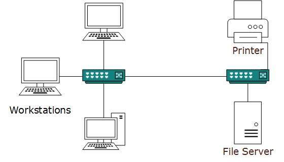 LANs are composed of inexpensive networking and routing equipment.
It may contains local servers serving file storage and other locally
shared applications. It mostly operates on private IP addresses and
does not involve heavy routing. LAN works under its own local domain
and controlled centrally.
LANs are composed of inexpensive networking and routing equipment.
It may contains local servers serving file storage and other locally
shared applications. It mostly operates on private IP addresses and
does not involve heavy routing. LAN works under its own local domain
and controlled centrally.LAN uses either Ethernet or Token-ring technology. Ethernet is most widely employed LAN technology and uses Star topology, while Token-ring is rarely seen.
LAN can be wired,wireless, or in both forms at once.
Metropolitan Area Network
The Metropolitan Area Network (MAN) generally expands throughout a city such as cable TV network. It can be in the form of Ethernet,Token-ring, ATM, or Fiber Distributed Data Interface (FDDI).Metro Ethernet is a service which is provided by ISPs. This service enables its users to expand their Local Area Networks. For example, MAN can help an organization to connect all of its offices in a city.
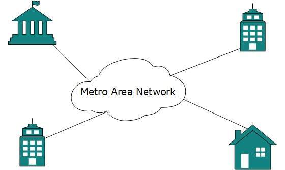 Backbone of MAN is high-capacity and high-speed fiber optics. MAN
works in between Local Area Network and Wide Area Network. MAN provides
uplink for LANs to WANs or internet.
Backbone of MAN is high-capacity and high-speed fiber optics. MAN
works in between Local Area Network and Wide Area Network. MAN provides
uplink for LANs to WANs or internet.Wide Area Network
As the name suggests,the Wide Area Network (WAN) covers a wide area which may span across provinces and even a whole country. Generally, telecommunication networks are Wide Area Network. These networks provide connectivity to MANs and LANs. Since they are equipped with very high speed backbone, WANs use very expensive network equipment.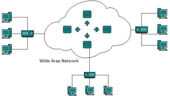 WAN may use advanced technologies such as Asynchronous Transfer Mode
(ATM), Frame Relay, and Synchronous Optical Network (SONET). WAN may be
managed by multiple administration.
WAN may use advanced technologies such as Asynchronous Transfer Mode
(ATM), Frame Relay, and Synchronous Optical Network (SONET). WAN may be
managed by multiple administration.Internetwork
A network of networks is called an internetwork, or simply the internet. It is the largest network in existence on this planet.The internet hugely connects all WANs and it can have connection to LANs and Home networks. Internet uses TCP/IP protocol suite and uses IP as its addressing protocol. Present day, Internet is widely implemented using IPv4. Because of shortage of address spaces, it is gradually migrating from IPv4 to IPv6.Internet enables its users to share and access enormous amount of information worldwide. It uses WWW, FTP, email services, audio and video streaming etc. At huge level, internet works on Client-Server model.
Internet uses very high speed backbone of fiber optics. To inter-connect various continents, fibers are laid under sea known to us as submarine communication cable.
Internet is widely deployed on World Wide Web services using HTML linked pages and is accessible by client software known as Web Browsers. When a user requests a page using some web browser located on some Web Server anywhere in the world, the Web Server responds with the proper HTML page. The communication delay is very low.
Internet is serving many proposes and is involved in many aspects of life. Some of them are:
- Web sites
- Instant Messaging
- Blogging
- Social Media
- Marketing
- Networking
- Resource Sharing
- Audio and Video Streaming
LAN technologies in brief:
Ethernet
Ethernet is a widely deployed LAN technology.This technology was invented by Bob Metcalfe and D.R. Boggs in the year 1970. It was standardized in IEEE 802.3 in 1980.Ethernet shares media. Network which uses shared media has high probability of data collision. Ethernet uses Carrier Sense Multi Access/Collision Detection (CSMA/CD) technology to detect collisions. On the occurrence of collision in Ethernet, all its hosts roll back, wait for some random amount of time, and then re-transmit the data.
Ethernet connector is,network interface card equipped with 48-bits MAC address. This helps other Ethernet devices to identify and communicate with remote devices in Ethernet.
Traditional Ethernet uses 10BASE-T specifications.The number 10 depicts 10MBPS speed, BASE stands for baseband, and T stands for Thick Ethernet. 10BASE-T Ethernet provides transmission speed up to 10MBPS and uses coaxial cable or Cat-5 twisted pair cable with RJ-45 connector. Ethernet follows star topology with segment length up to 100 meters. All devices are connected to a hub/switch in a star fashion.
Fast-Ethernet
To encompass need of fast emerging software and hardware technologies, Ethernet extends itself as Fast-Ethernet. It can run on UTP, Optical Fiber, and wirelessly too. It can provide speed up to 100 MBPS. This standard is named as 100BASE-T in IEEE 803.2 using Cat-5 twisted pair cable. It uses CSMA/CD technique for wired media sharing among the Ethernet hosts and CSMA/CA (CA stands for Collision Avoidance) technique for wireless Ethernet LAN.Fast Ethernet on fiber is defined under 100BASE-FX standard which provides speed up to 100 MBPS on fiber. Ethernet over fiber can be extended up to 100 meters in half-duplex mode and can reach maximum of 2000 meters in full-duplex over multimode fibers.
Giga-Ethernet
After being introduced in 1995, Fast-Ethernet could enjoy its high speed status only for 3 years till Giga-Ethernet introduced. Giga-Ethernet provides speed up to 1000 mbits/seconds. IEEE802.3ab standardize Giga-Ethernet over UTP using Cat-5, Cat-5e and Cat-6 cables. IEEE802.3ah defines Giga-Ethernet over Fiber.Virtual LAN
LAN uses Ethernet which in turn works on shared media. Shared media in Ethernet create one single Broadcast domain and one single Collision domain. Introduction of switches to Ethernet has removed single collision domain issue and each device connected to switch works in its separate collision domain. But even Switches cannot divide a network into separate Broadcast domains.Virtual LAN is a solution to divide a single Broadcast domain into multiple Broadcast domains. Host in one VLAN cannot speak to a host in another. By default, all hosts are placed into the same VLAN.
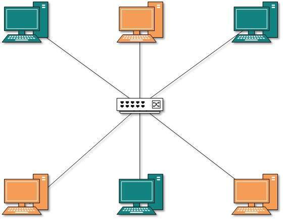 In this diagram, different VLANs are depicted in different color
codes. Hosts in one VLAN, even if connected on the same Switch cannot
see or speak to other hosts in different VLANs. VLAN is Layer-2
technology which works closely on Ethernet. To route packets between
two different VLANs a Layer-3 device such as Router is required.
In this diagram, different VLANs are depicted in different color
codes. Hosts in one VLAN, even if connected on the same Switch cannot
see or speak to other hosts in different VLANs. VLAN is Layer-2
technology which works closely on Ethernet. To route packets between
two different VLANs a Layer-3 device such as Router is required.Point-to-Point
Point-to-point networks contains exactly two hosts such as computer, switches or routers, servers connected back to back using a single piece of cable. Often, the receiving end of one host is connected to sending end of the other and vice-versa.
Bus Topology
In case of Bus topology, all devices share single communication line or cable.Bus topology may have problem while multiple hosts sending data at the same time. Therefore, Bus topology either uses CSMA/CD technology or recognizes one host as Bus Master to solve the issue. It is one of the simple forms of networking where a failure of a device does not affect the other devices. But failure of the shared communication line can make all other devices stop functioning.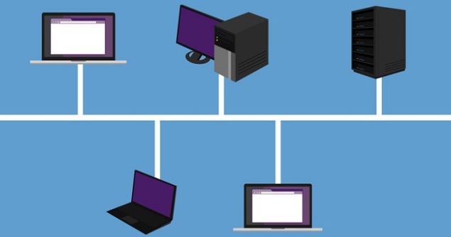 Both ends of the shared channel have line terminator. The data is
sent in only one direction and as soon as it reaches the extreme end,
the terminator removes the data from the line.
Both ends of the shared channel have line terminator. The data is
sent in only one direction and as soon as it reaches the extreme end,
the terminator removes the data from the line.Star Topology
All hosts in Star topology are connected to a central device, known as hub device, using a point-to-point connection. That is, there exists a point to point connection between hosts and hub. The hub device can be any of the following:- Layer-1 device such as hub or repeater
- Layer-2 device such as switch or bridge
- Layer-3 device such as router or gateway
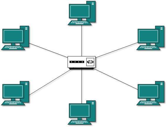 As in Bus topology, hub acts as single point of failure. If hub
fails, connectivity of all hosts to all other hosts fails. Every
communication between hosts, takes place through only the hub.Star
topology is not expensive as to connect one more host, only one cable is
required and configuration is simple.
As in Bus topology, hub acts as single point of failure. If hub
fails, connectivity of all hosts to all other hosts fails. Every
communication between hosts, takes place through only the hub.Star
topology is not expensive as to connect one more host, only one cable is
required and configuration is simple.Ring Topology
In ring topology, each host machine connects to exactly two other machines, creating a circular network structure. When one host tries to communicate or send message to a host which is not adjacent to it, the data travels through all intermediate hosts. To connect one more host in the existing structure, the administrator may need only one more extra cable.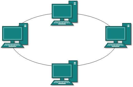 Failure of any host results in failure of the whole ring.Thus, every
connection in the ring is a point of failure. There are methods which
employ one more backup ring.
Failure of any host results in failure of the whole ring.Thus, every
connection in the ring is a point of failure. There are methods which
employ one more backup ring.Mesh Topology
In this type of topology, a host is connected to one or multiple hosts.This topology has hosts in point-to-point connection with every other host or may also have hosts which are in point-to-point connection to few hosts only.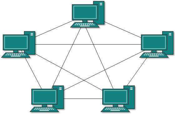 Hosts in Mesh topology also work as relay for other hosts which do
not have direct point-to-point links. Mesh technology comes into two
types:
Hosts in Mesh topology also work as relay for other hosts which do
not have direct point-to-point links. Mesh technology comes into two
types:- Full Mesh: All hosts have a point-to-point connection to every other host in the network. Thus for every new host n(n-1)/2 connections are required. It provides the most reliable network structure among all network topologies.
- Partially Mesh: Not all hosts have point-to-point connection to every other host. Hosts connect to each other in some arbitrarily fashion. This topology exists where we need to provide reliability to some hosts out of all.
Tree Topology
Also known as Hierarchical Topology, this is the most common form of network topology in use presently.This topology imitates as extended Star topology and inherits properties of bus topology.This topology divides the network in to multiple levels/layers of network. Mainly in LANs, a network is bifurcated into three types of network devices. The lowermost is access-layer where computers are attached. The middle layer is known as distribution layer, which works as mediator between upper layer and lower layer. The highest layer is known as core layer, and is central point of the network, i.e. root of the tree from which all nodes fork.
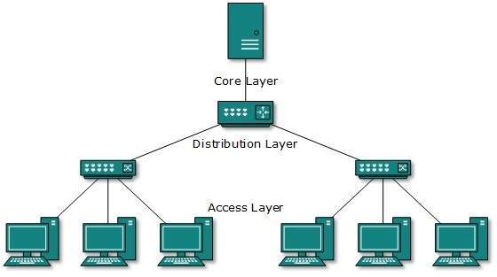 All neighboring hosts have point-to-point connection between
them.Similar to the Bus topology, if the root goes down, then the entire
network suffers even.though it is not the single point of failure.
Every connection serves as point of failure, failing of which divides
the network into unreachable segment.
All neighboring hosts have point-to-point connection between
them.Similar to the Bus topology, if the root goes down, then the entire
network suffers even.though it is not the single point of failure.
Every connection serves as point of failure, failing of which divides
the network into unreachable segment.Daisy Chain
This topology connects all the hosts in a linear fashion. Similar to Ring topology, all hosts are connected to two hosts only, except the end hosts.Means, if the end hosts in daisy chain are connected then it represents Ring topology. Each link in daisy chain topology represents single point of failure.
Every link failure splits the network into two segments.Every
intermediate host works as relay for its immediate hosts.
Each link in daisy chain topology represents single point of failure.
Every link failure splits the network into two segments.Every
intermediate host works as relay for its immediate hosts.Hybrid Topology
A network structure whose design contains more than one topology is said to be hybrid topology. Hybrid topology inherits merits and demerits of all the incorporating topologies.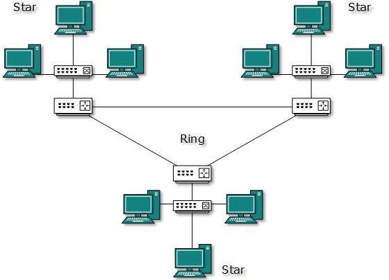 The above picture represents an arbitrarily hybrid topology. The
combining topologies may contain attributes of Star, Ring, Bus, and
Daisy-chain topologies. Most WANs are connected by means of Dual-Ring
topology and networks connected to them are mostly Star topology
networks. Internet is the best example of largest Hybrid topology
The above picture represents an arbitrarily hybrid topology. The
combining topologies may contain attributes of Star, Ring, Bus, and
Daisy-chain topologies. Most WANs are connected by means of Dual-Ring
topology and networks connected to them are mostly Star topology
networks. Internet is the best example of largest Hybrid topologyLayered Tasks
In layered architecture of Network Model, one whole network process is divided into small tasks. Each small task is then assigned to a particular layer which works dedicatedly to process the task only. Every layer does only specific work.In layered communication system, one layer of a host deals with the task done by or to be done by its peer layer at the same level on the remote host. The task is either initiated by layer at the lowest level or at the top most level. If the task is initiated by the-top most layer, it is passed on to the layer below it for further processing. The lower layer does the same thing, it processes the task and passes on to lower layer. If the task is initiated by lower most layer, then the reverse path is taken.
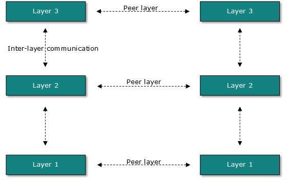 Every layer clubs together all procedures, protocols, and methods
which it requires to execute its piece of task. All layers identify
their counterparts by means of encapsulation header and tail.
Every layer clubs together all procedures, protocols, and methods
which it requires to execute its piece of task. All layers identify
their counterparts by means of encapsulation header and tail.OSI Model
Open System Interconnect is an open standard for all communication systems. OSI model is established by International Standard Organization (ISO). This model has seven layers: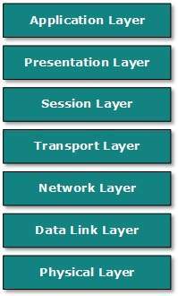
- Application Layer: This layer is responsible for providing interface to the application user. This layer encompasses protocols which directly interact with the user.
- Presentation Layer: This layer defines how data in the native format of remote host should be presented in the native format of host.
- Session Layer: This layer maintains sessions between remote hosts. For example, once user/password authentication is done, the remote host maintains this session for a while and does not ask for authentication again in that time span.
- Transport Layer: This layer is responsible for end-to-end delivery between hosts.
- Network Layer: This layer is responsible for address assignment and uniquely addressing hosts in a network.
- Data Link Layer: This layer is responsible for reading and writing data from and onto the line. Link errors are detected at this layer.
- Physical Layer: This layer defines the hardware, cabling wiring, power output, pulse rate etc.
Internet Model
Internet uses TCP/IP protocol suite, also known as Internet suite. This defines Internet Model which contains four layered architecture. OSI Model is general communication model but Internet Model is what the internet uses for all its communication.The internet is independent of its underlying network architecture so is its Model. This model has the following layers: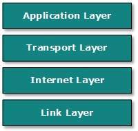
- Application Layer: This layer defines the protocol which enables user to interact with the network.For example, FTP, HTTP etc.
- Transport Layer: This layer defines how data should flow between hosts. Major protocol at this layer is Transmission Control Protocol (TCP). This layer ensures data delivered between hosts is in-order and is responsible for end-to-end delivery.
- Internet Layer: Internet Protocol (IP) works on this layer. This layer facilitates host addressing and recognition. This layer defines routing.
- Link Layer: This layer provides mechanism of sending and receiving actual data.Unlike its OSI Model counterpart, this layer is independent of underlying network architecture and hardware.
All security threats are intentional i.e. they occur only if intentionally triggered. Security threats can be divided into the following categories:
- Interruption
Interruption is a security threat in which availability of resources is attacked. For example, a user is unable to access its web-server or the web-server is hijacked. - Privacy-Breach
In this threat, the privacy of a user is compromised. Someone, who is not the authorized person is accessing or intercepting data sent or received by the original authenticated user. - Integrity
This type of threat includes any alteration or modification in the original context of communication. The attacker intercepts and receives the data sent by the sender and the attacker then either modifies or generates false data and sends to the receiver. The receiver receives the data assuming that it is being sent by the original Sender. - Authenticity
This threat occurs when an attacker or a security violator, poses as a genuine person and accesses the resources or communicates with other genuine users.
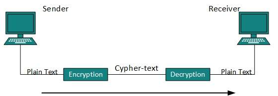 Cryptography is a technique to encrypt the plain-text data which
makes it difficult to understand and interpret. There are several
cryptographic algorithms available present day as described below:
Cryptography is a technique to encrypt the plain-text data which
makes it difficult to understand and interpret. There are several
cryptographic algorithms available present day as described below:- Secret Key
- Public Key
- Message Digest
Secret Key Encryption
Both sender and receiver have one secret key. This secret key is used to encrypt the data at sender’s end. After the data is encrypted, it is sent on the public domain to the receiver. Because the receiver knows and has the Secret Key, the encrypted data packets can easily be decrypted.Example of secret key encryption is Data Encryption Standard (DES). In Secret Key encryption, it is required to have a separate key for each host on the network making it difficult to manage.
Public Key Encryption
In this encryption system, every user has its own Secret Key and it is not in the shared domain. The secret key is never revealed on public domain. Along with secret key, every user has its own but public key. Public key is always made public and is used by Senders to encrypt the data. When the user receives the encrypted data, he can easily decrypt it by using its own Secret Key.Example of public key encryption is Rivest-Shamir-Adleman (RSA).
Message Digest
In this method, actual data is not sent, instead a hash value is calculated and sent. The other end user, computes its own hash value and compares with the one just received.If both hash values are matched, then it is accepted otherwise rejected.Example of Message Digest is MD5 hashing. It is mostly used in authentication where user password is cross checked with the one saved on the server.
Physical layer provides its services to Data-link layer. Data-link layer hands over frames to physical layer. Physical layer converts them to electrical pulses, which represent binary data.The binary data is then sent over the wired or wireless media.
Signals
When data is sent over physical medium, it needs to be first converted into electromagnetic signals. Data itself can be analog such as human voice, or digital such as file on the disk.Both analog and digital data can be represented in digital or analog signals.- Digital Signals
Digital signals are discrete in nature and represent sequence of voltage pulses. Digital signals are used within the circuitry of a computer system. - Analog Signals
Analog signals are in continuous wave form in nature and represented by continuous electromagnetic waves.
Transmission Impairment
When signals travel through the medium they tend to deteriorate. This may have many reasons as given:- Attenuation
For the receiver to interpret the data accurately, the signal must be sufficiently strong.When the signal passes through the medium, it tends to get weaker.As it covers distance, it loses strength. - Dispersion
As signal travels through the media, it tends to spread and overlaps. The amount of dispersion depends upon the frequency used. - Delay distortion
Signals are sent over media with pre-defined speed and frequency. If the signal speed and frequency do not match, there are possibilities that signal reaches destination in arbitrary fashion. In digital media, this is very critical that some bits reach earlier than the previously sent ones. - Noise
Random disturbance or fluctuation in analog or digital signal is said to be Noise in signal, which may distort the actual information being carried. Noise can be characterized in one of the following class:
- Thermal Noise
Heat agitates the electronic conductors of a medium which may introduce noise in the media. Up to a certain level, thermal noise is unavoidable. - Intermodulation
When multiple frequencies share a medium, their interference can cause noise in the medium. Intermodulation noise occurs if two different frequencies are sharing a medium and one of them has excessive strength or the component itself is not functioning properly, then the resultant frequency may not be delivered as expected. - Crosstalk
This sort of noise happens when a foreign signal enters into the media. This is because signal in one medium affects the signal of second medium. - Impulse
This noise is introduced because of irregular disturbances such as lightening, electricity, short-circuit, or faulty components. Digital data is mostly affected by this sort of noise.
- Thermal Noise
Transmission Media
The media over which the information between two computer systems is sent, called transmission media. Transmission media comes in two forms.- Guided Media
All communication wires/cables are guided media, such as UTP, coaxial cables, and fiber Optics. In this media, the sender and receiver are directly connected and the information is send (guided) through it. - Unguided Media
Wireless or open air space is said to be unguided media, because there is no connectivity between the sender and receiver. Information is spread over the air, and anyone including the actual recipient may collect the information.
Channel Capacity
The speed of transmission of information is said to be the channel capacity. We count it as data rate in digital world. It depends on numerous factors such as:- Bandwidth: The physical limitation of underlying media.
- Error-rate: Incorrect reception of information because of noise.
- Encoding: The number of levels used for signaling.
Multiplexing
Multiplexing is a technique to mix and send multiple data streams over a single medium. This technique requires system hardware called multiplexer (MUX) for multiplexing the streams and sending them on a medium, and de-multiplexer (DMUX) which takes information from the medium and distributes to different destinations.Switching
Switching is a mechanism by which data/information sent from source towards destination which are not directly connected. Networks have interconnecting devices, which receives data from directly connected sources, stores data, analyze it and then forwards to the next interconnecting device closest to the destination.Switching can be categorized as:
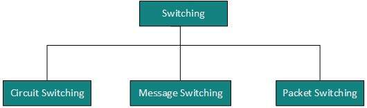
Digital-to-Digital Conversion
This section explains how to convert digital data into digital signals. It can be done in two ways, line coding and block coding. For all communications, line coding is necessary whereas block coding is optional.Line Coding
The process for converting digital data into digital signal is said to be Line Coding. Digital data is found in binary format.It is represented (stored) internally as series of 1s and 0s.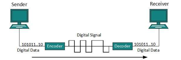 Digital signal is denoted by discreet signal, which represents
digital data.There are three types of line coding schemes available:
Digital signal is denoted by discreet signal, which represents
digital data.There are three types of line coding schemes available: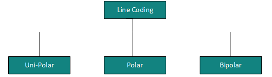
Uni-polar Encoding
Unipolar encoding schemes use single voltage level to represent data. In this case, to represent binary 1, high voltage is transmitted and to represent 0, no voltage is transmitted. It is also called Unipolar-Non-return-to-zero, because there is no rest condition i.e. it either represents 1 or 0.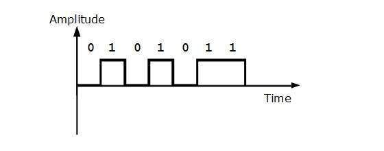
Polar Encoding
Polar encoding scheme uses multiple voltage levels to represent binary values. Polar encodings is available in four types:- Polar Non-Return to Zero (Polar NRZ)
It uses two different voltage levels to represent binary values. Generally, positive voltage represents 1 and negative value represents 0. It is also NRZ because there is no rest condition.
NRZ scheme has two variants: NRZ-L and NRZ-I.
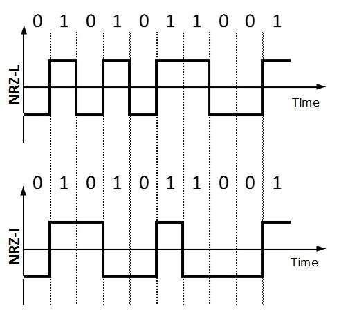 NRZ-L changes voltage level at when a different bit is encountered whereas NRZ-I changes voltage when a 1 is encountered.
 Return to Zero (RZ)
Problem with NRZ is that the receiver cannot conclude when a bit ended and when the next bit is started, in case when sender and receiver’s clock are not synchronized.
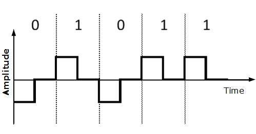 RZ uses three voltage levels, positive voltage to represent 1,
negative voltage to represent 0 and zero voltage for none. Signals
change during bits not between bits.
RZ uses three voltage levels, positive voltage to represent 1,
negative voltage to represent 0 and zero voltage for none. Signals
change during bits not between bits.Manchester
This encoding scheme is a combination of RZ and NRZ-L. Bit time is divided into two halves. It transits in the middle of the bit and changes phase when a different bit is encountered.Differential Manchester
This encoding scheme is a combination of RZ and NRZ-I. It also transit at the middle of the bit but changes phase only when 1 is encountered.
Bipolar Encoding
Bipolar encoding uses three voltage levels, positive, negative and zero. Zero voltage represents binary 0 and bit 1 is represented by altering positive and negative voltages.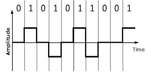
Block Coding
To ensure accuracy of the received data frame redundant bits are used. For example, in even-parity, one parity bit is added to make the count of 1s in the frame even. This way the original number of bits is increased. It is called Block Coding.Block coding is represented by slash notation, mB/nB.Means, m-bit block is substituted with n-bit block where n > m. Block coding involves three steps:
- Division,
- Substitution
- Combination.
Analog-to-Digital Conversion
Microphones create analog voice and camera creates analog videos, which are treated is analog data. To transmit this analog data over digital signals, we need analog to digital conversion.Analog data is a continuous stream of data in the wave form whereas digital data is discrete. To convert analog wave into digital data, we use Pulse Code Modulation (PCM).
PCM is one of the most commonly used method to convert analog data into digital form. It involves three steps:
- Sampling
- Quantization
- Encoding.
Sampling
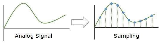 The analog signal is sampled every T interval. Most important factor
in sampling is the rate at which analog signal is sampled. According
to Nyquist Theorem, the sampling rate must be at least two times of the
highest frequency of the signal.
The analog signal is sampled every T interval. Most important factor
in sampling is the rate at which analog signal is sampled. According
to Nyquist Theorem, the sampling rate must be at least two times of the
highest frequency of the signal.Quantization
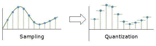 Sampling yields discrete form of continuous analog signal. Every
discrete pattern shows the amplitude of the analog signal at that
instance. The quantization is done between the maximum amplitude value
and the minimum amplitude value. Quantization is approximation of the
instantaneous analog value.
Sampling yields discrete form of continuous analog signal. Every
discrete pattern shows the amplitude of the analog signal at that
instance. The quantization is done between the maximum amplitude value
and the minimum amplitude value. Quantization is approximation of the
instantaneous analog value.Encoding
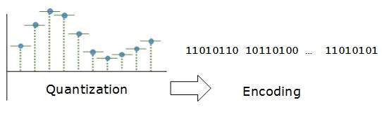 In encoding, each approximated value is then converted into binary format.
Transmission Modes
The transmission mode decides how data is transmitted between two computers.The binary data in the form of 1s and 0s can be sent in two different modes: Parallel and Serial.Parallel Transmission
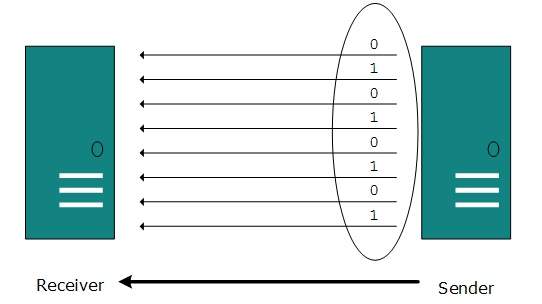 The binary bits are organized in-to groups of fixed length. Both
sender and receiver are connected in parallel with the equal number of
data lines. Both computers distinguish between high order and low order
data lines. The sender sends all the bits at once on all lines.Because
the data lines are equal to the number of bits in a group or data
frame, a complete group of bits (data frame) is sent in one go.
Advantage of Parallel transmission is high speed and disadvantage is the
cost of wires, as it is equal to the number of bits sent in parallel.
The binary bits are organized in-to groups of fixed length. Both
sender and receiver are connected in parallel with the equal number of
data lines. Both computers distinguish between high order and low order
data lines. The sender sends all the bits at once on all lines.Because
the data lines are equal to the number of bits in a group or data
frame, a complete group of bits (data frame) is sent in one go.
Advantage of Parallel transmission is high speed and disadvantage is the
cost of wires, as it is equal to the number of bits sent in parallel.Serial Transmission
In serial transmission, bits are sent one after another in a queue manner. Serial transmission requires only one communication channel.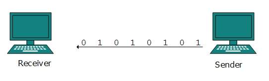 Serial transmission can be either asynchronous or synchronous.
Asynchronous Serial Transmission
It is named so because there’is no importance of timing. Data-bits have specific pattern and they help receiver recognize the start and end data bits.For example, a 0 is prefixed on every data byte and one or more 1s are added at the end.Two continuous data-frames (bytes) may have a gap between them.
Synchronous Serial Transmission
Timing in synchronous transmission has importance as there is no mechanism followed to recognize start and end data bits.There is no pattern or prefix/suffix method. Data bits are sent in burst mode without maintaining gap between bytes (8-bits). Single burst of data bits may contain a number of bytes. Therefore, timing becomes very important.It is up to the receiver to recognize and separate bits into bytes.The advantage of synchronous transmission is high speed, and it has no overhead of extra header and footer bits as in asynchronous transmission.
Bandpass:The filters are used to filter and pass frequencies of interest. A bandpass is a band of frequencies which can pass the filter.
Low-pass: Low-pass is a filter that passes low frequencies signals.
When digital data is converted into a bandpass analog signal, it is called digital-to-analog conversion. When low-pass analog signal is converted into bandpass analog signal, it is called analog-to-analog conversion.
Digital-to-Analog Conversion
When data from one computer is sent to another via some analog carrier, it is first converted into analog signals. Analog signals are modified to reflect digital data.An analog signal is characterized by its amplitude, frequency, and phase. There are three kinds of digital-to-analog conversions:
- Amplitude Shift Keying
In this conversion technique, the amplitude of analog carrier signal is modified to reflect binary data.
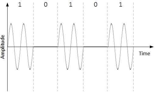 When binary data represents digit 1, the amplitude is held; otherwise
it is set to 0. Both frequency and phase remain same as in the
original carrier signal.
When binary data represents digit 1, the amplitude is held; otherwise
it is set to 0. Both frequency and phase remain same as in the
original carrier signal. - Frequency Shift Keying
In this conversion technique, the frequency of the analog carrier signal is modified to reflect binary data.
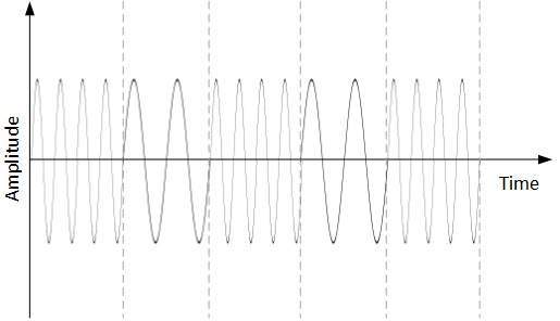 This technique uses two frequencies, f1 and f2. One of them, for
example f1, is chosen to represent binary digit 1 and the other one is
used to represent binary digit 0. Both amplitude and phase of the
carrier wave are kept intact.
This technique uses two frequencies, f1 and f2. One of them, for
example f1, is chosen to represent binary digit 1 and the other one is
used to represent binary digit 0. Both amplitude and phase of the
carrier wave are kept intact. - Phase Shift Keying
In this conversion scheme, the phase of the original carrier signal is altered to reflect the binary data.
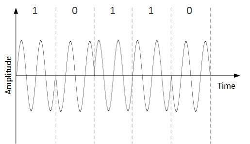 When a new binary symbol is encountered, the phase of the signal is
altered. Amplitude and frequency of the original carrier signal is kept
intact.
When a new binary symbol is encountered, the phase of the signal is
altered. Amplitude and frequency of the original carrier signal is kept
intact.
- Quadrature Phase Shift Keying
QPSK alters the phase to reflect two binary digits at once. This is done in two different phases. The main stream of binary data is divided equally into two sub-streams. The serial data is converted in to parallel in both sub-streams and then each stream is converted to digital signal using NRZ technique. Later, both the digital signals are merged together.
Analog-to-Analog Conversion
Analog signals are modified to represent analog data. This conversion is also known as Analog Modulation. Analog modulation is required when bandpass is used. Analog to analog conversion can be done in three ways: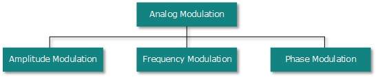
- Amplitude Modulation
In this modulation, the amplitude of the carrier signal is modified to reflect the analog data.
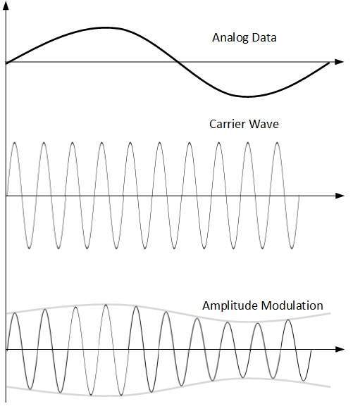 Amplitude modulation is implemented by means of a multiplier. The
amplitude of modulating signal (analog data) is multiplied by the
amplitude of carrier frequency, which then reflects analog data.
Amplitude modulation is implemented by means of a multiplier. The
amplitude of modulating signal (analog data) is multiplied by the
amplitude of carrier frequency, which then reflects analog data.
The frequency and phase of carrier signal remain unchanged. - Frequency Modulation
In this modulation technique, the frequency of the carrier signal is modified to reflect the change in the voltage levels of the modulating signal (analog data).
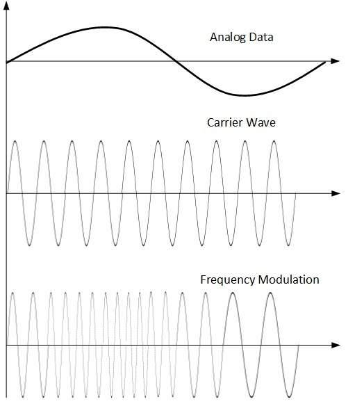 The amplitude and phase of the carrier signal are not altered.
 - Phase Modulation
In the modulation technique, the phase of carrier signal is modulated in order to reflect the change in voltage (amplitude) of analog data signal.
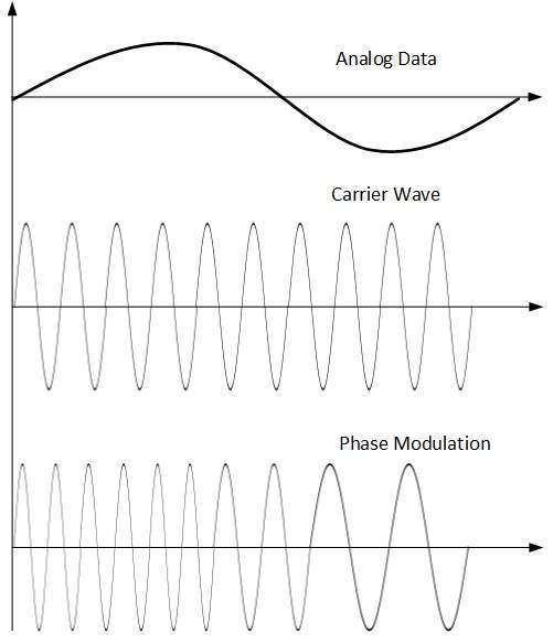 Phase modulation is practically similar to Frequency Modulation, but
in Phase modulation frequency of the carrier signal is not increased.
Frequency of carrier is signal is changed (made dense and sparse) to
reflect voltage change in the amplitude of modulating signal.
Phase modulation is practically similar to Frequency Modulation, but
in Phase modulation frequency of the carrier signal is not increased.
Frequency of carrier is signal is changed (made dense and sparse) to
reflect voltage change in the amplitude of modulating signal.
Magnetic Media
One of the most convenient way to transfer data from one computer to another, even before the birth of networking, was to save it on some storage media and transfer physical from one station to another. Though it may seem old-fashion way in today’s world of high speed internet, but when the size of data is huge, the magnetic media comes into play.For example, a bank has to handle and transfer huge data of its customer, which stores a backup of it at some geographically far-away place for security reasons and to keep it from uncertain calamities. If the bank needs to store its huge backup data then its,transfer through internet is not feasible.The WAN links may not support such high speed.Even if they do; the cost too high to afford.
In these cases, data backup is stored onto magnetic tapes or magnetic discs, and then shifted physically at remote places.
Twisted Pair Cable
A twisted pair cable is made of two plastic insulated copper wires twisted together to form a single media. Out of these two wires, only one carries actual signal and another is used for ground reference. The twists between wires are helpful in reducing noise (electro-magnetic interference) and crosstalk. There are two types of twisted pair cables:
- Shielded Twisted Pair (STP) Cable
- Unshielded Twisted Pair (UTP) Cable
UTP has seven categories, each suitable for specific use. In computer networks, Cat-5, Cat-5e, and Cat-6 cables are mostly used. UTP cables are connected by RJ45 connectors.
Coaxial Cable
Coaxial cable has two wires of copper. The core wire lies in the center and it is made of solid conductor.The core is enclosed in an insulating sheath.The second wire is wrapped around over the sheath and that too in turn encased by insulator sheath.This all is covered by plastic cover. Because of its structure,the coax cable is capable of carrying high
frequency signals than that of twisted pair cable.The wrapped structure
provides it a good shield against noise and cross talk. Coaxial cables
provide high bandwidth rates of up to 450 mbps.
Because of its structure,the coax cable is capable of carrying high
frequency signals than that of twisted pair cable.The wrapped structure
provides it a good shield against noise and cross talk. Coaxial cables
provide high bandwidth rates of up to 450 mbps.There are three categories of coax cables namely, RG-59 (Cable TV), RG-58 (Thin Ethernet), and RG-11 (Thick Ethernet). RG stands for Radio Government.
Cables are connected using BNC connector and BNC-T. BNC terminator is used to terminate the wire at the far ends.
Power Lines
Power Line communication (PLC) is Layer-1 (Physical Layer) technology which uses power cables to transmit data signals.In PLC, modulated data is sent over the cables. The receiver on the other end de-modulates and interprets the data.Because power lines are widely deployed, PLC can make all powered devices controlled and monitored. PLC works in half-duplex.
There are two types of PLC:
- Narrow band PLC
- Broad band PLC
Broadband PLC provides higher data rates up to 100s of Mbps and works at higher frequencies (1.8 – 250 MHz).They cannot be as much extended as Narrowband PLC.
Fiber Optics
Fiber Optic works on the properties of light. When light ray hits at critical angle it tends to refracts at 90 degree. This property has been used in fiber optic. The core of fiber optic cable is made of high quality glass or plastic. From one end of it light is emitted, it travels through it and at the other end light detector detects light stream and converts it to electric data.Fiber Optic provides the highest mode of speed. It comes in two modes, one is single mode fiber and second is multimode fiber. Single mode fiber can carry a single ray of light whereas multimode is capable of carrying multiple beams of light.
 Fiber Optic also comes in unidirectional and bidirectional
capabilities. To connect and access fiber optic special type of
connectors are used. These can be Subscriber Channel (SC), Straight Tip
(ST), or MT-RJ.
Fiber Optic also comes in unidirectional and bidirectional
capabilities. To connect and access fiber optic special type of
connectors are used. These can be Subscriber Channel (SC), Straight Tip
(ST), or MT-RJ.When an antenna is attached to electrical circuit of a computer or wireless device, it converts the digital data into wireless signals and spread all over within its frequency range. The receptor on the other end receives these signals and converts them back to digital data.
A little part of electromagnetic spectrum can be used for wireless transmission.
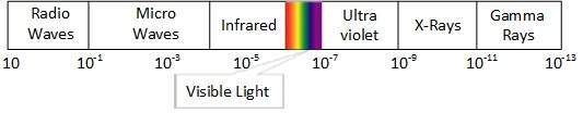
Radio Transmission
Radio frequency is easier to generate and because of its large wavelength it can penetrate through walls and structures alike.Radio waves can have wavelength from 1 mm – 100,000 km and have frequency ranging from 3 Hz (Extremely Low Frequency) to 300 GHz (Extremely High Frequency). Radio frequencies are sub-divided into six bands.Radio waves at lower frequencies can travel through walls whereas higher RF can travel in straight line and bounce back.The power of low frequency waves decreases sharply as they cover long distance. High frequency radio waves have more power.
Lower frequencies such as VLF, LF, MF bands can travel on the ground up to 1000 kilometers, over the earth’s surface.
 Radio waves of high frequencies are prone to be absorbed by rain and
other obstacles. They use Ionosphere of earth atmosphere. High
frequency radio waves such as HF and VHF bands are spread upwards. When
they reach Ionosphere, they are refracted back to the earth.
Radio waves of high frequencies are prone to be absorbed by rain and
other obstacles. They use Ionosphere of earth atmosphere. High
frequency radio waves such as HF and VHF bands are spread upwards. When
they reach Ionosphere, they are refracted back to the earth. 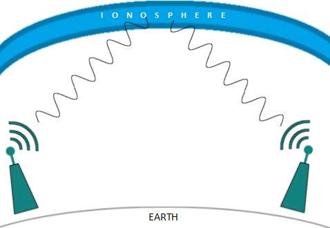
Microwave Transmission
Electromagnetic waves above 100 MHz tend to travel in a straight line and signals over them can be sent by beaming those waves towards one particular station. Because Microwaves travels in straight lines, both sender and receiver must be aligned to be strictly in line-of-sight.Microwaves can have wavelength ranging from 1 mm – 1 meter and frequency ranging from 300 MHz to 300 GHz.
 Microwave antennas concentrate the waves making a beam of it. As
shown in picture above, multiple antennas can be aligned to reach
farther. Microwaves have higher frequencies and do not penetrate wall
like obstacles.
Microwave antennas concentrate the waves making a beam of it. As
shown in picture above, multiple antennas can be aligned to reach
farther. Microwaves have higher frequencies and do not penetrate wall
like obstacles. Microwave transmission depends highly upon the weather conditions and the frequency it is using.
Infrared Transmission
Infrared wave lies in between visible light spectrum and microwaves. It has wavelength of 700-nm to 1-mm and frequency ranges from 300-GHz to 430-THz.Infrared wave is used for very short range communication purposes such as television and it’s remote. Infrared travels in a straight line hence it is directional by nature. Because of high frequency range, Infrared cannot cross wall-like obstacles.
Light Transmission
Highest most electromagnetic spectrum which can be used for data transmission is light or optical signaling. This is achieved by means of LASER.Because of frequency light uses, it tends to travel strictly in straight line.Hence the sender and receiver must be in the line-of-sight. Because laser transmission is unidirectional, at both ends of communication the laser and the photo-detector needs to be installed. Laser beam is generally 1mm wide hence it is a work of precision to align two far receptors each pointing to lasers source.
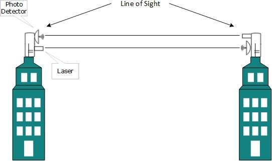 Laser works as Tx (transmitter) and photo-detectors works as Rx (receiver).
 Lasers cannot penetrate obstacles such as walls, rain, and thick fog. Additionally, laser beam is distorted by wind, atmosphere temperature, or variation in temperature in the path.
Laser is safe for data transmission as it is very difficult to tap 1mm wide laser without interrupting the communication channel.
Communication is possible over the air (radio frequency), using a physical media (cable), and light (optical fiber). All mediums are capable of multiplexing.
When multiple senders try to send over a single medium, a device called Multiplexer divides the physical channel and allocates one to each. On the other end of communication, a De-multiplexer receives data from a single medium, identifies each, and sends to different receivers.
Frequency Division Multiplexing
When the carrier is frequency, FDM is used. FDM is an analog technology. FDM divides the spectrum or carrier bandwidth in logical channels and allocates one user to each channel. Each user can use the channel frequency independently and has exclusive access of it. All channels are divided in such a way that they do not overlap with each other. Channels are separated by guard bands. Guard band is a frequency which is not used by either channel.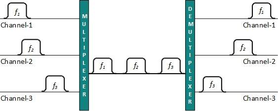
Time Division Multiplexing
TDM is applied primarily on digital signals but can be applied on analog signals as well. In TDM the shared channel is divided among its user by means of time slot. Each user can transmit data within the provided time slot only. Digital signals are divided in frames, equivalent to time slot i.e. frame of an optimal size which can be transmitted in given time slot.TDM works in synchronized mode. Both ends, i.e. Multiplexer and De-multiplexer are timely synchronized and both switch to next channel simultaneously.
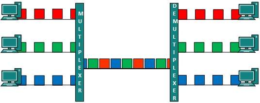 When channel A transmits its frame at one end,the De-multiplexer
provides media to channel A on the other end.As soon as the channel A’s
time slot expires, this side switches to channel B. On the other end,
the De-multiplexer works in a synchronized manner and provides media to
channel B. Signals from different channels travel the path in
interleaved manner.
When channel A transmits its frame at one end,the De-multiplexer
provides media to channel A on the other end.As soon as the channel A’s
time slot expires, this side switches to channel B. On the other end,
the De-multiplexer works in a synchronized manner and provides media to
channel B. Signals from different channels travel the path in
interleaved manner.Wavelength Division Multiplexing
Light has different wavelength (colors). In fiber optic mode, multiple optical carrier signals are multiplexed into an optical fiber by using different wavelengths. This is an analog multiplexing technique and is done conceptually in the same manner as FDM but uses light as signals.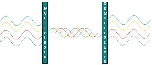 Further, on each wavelength time division multiplexing can be incorporated to accommodate more data signals.
Code Division Multiplexing
Multiple data signals can be transmitted over a single frequency by using Code Division Multiplexing. FDM divides the frequency in smaller channels but CDM allows its users to full bandwidth and transmit signals all the time using a unique code. CDM uses orthogonal codes to spread signals.Each station is assigned with a unique code, called chip. Signals travel with these codes independently, inside the whole bandwidth.The receiver knows in advance the chip code signal it has to receive.
- Connectionless: The data is forwarded on behalf of forwarding tables. No previous handshaking is required and acknowledgements are optional.
- Connection Oriented: Before switching data to be forwarded to destination, there is a need to pre-establish circuit along the path between both endpoints. Data is then forwarded on that circuit. After the transfer is completed, circuits can be kept for future use or can be turned down immediately.
Circuit Switching
When two nodes communicate with each other over a dedicated communication path, it is called circuit switching.There 'is a need of pre-specified route from which data will travels and no other data is permitted.In circuit switching, to transfer the data, circuit must be established so that the data transfer can take place.Circuits can be permanent or temporary. Applications which use circuit switching may have to go through three phases:
- Establish a circuit
- Transfer the data
- Disconnect the circuit
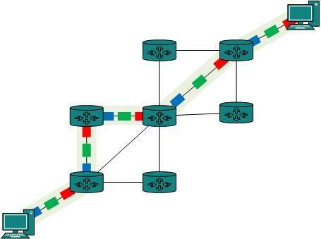 Circuit switching was designed for voice applications. Telephone is
the best suitable example of circuit switching. Before a user can make a
call, a virtual path between caller and callee is established over the
network.
Circuit switching was designed for voice applications. Telephone is
the best suitable example of circuit switching. Before a user can make a
call, a virtual path between caller and callee is established over the
network.Message Switching
This technique was somewhere in middle of circuit switching and packet switching. In message switching, the whole message is treated as a data unit and is switching / transferred in its entirety.A switch working on message switching, first receives the whole message and buffers it until there are resources available to transfer it to the next hop. If the next hop is not having enough resource to accommodate large size message, the message is stored and switch waits.
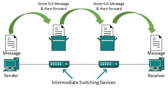 This technique was considered substitute to circuit switching. As in
circuit switching the whole path is blocked for two entities only.
Message switching is replaced by packet switching. Message switching
has the following drawbacks:
This technique was considered substitute to circuit switching. As in
circuit switching the whole path is blocked for two entities only.
Message switching is replaced by packet switching. Message switching
has the following drawbacks:- Every switch in transit path needs enough storage to accommodate entire message.
- Because of store-and-forward technique and waits included until resources are available, message switching is very slow.
- Message switching was not a solution for streaming media and real-time applications.
Packet Switching
Shortcomings of message switching gave birth to an idea of packet switching. The entire message is broken down into smaller chunks called packets. The switching information is added in the header of each packet and transmitted independently.It is easier for intermediate networking devices to store small size packets and they do not take much resources either on carrier path or in the internal memory of switches.
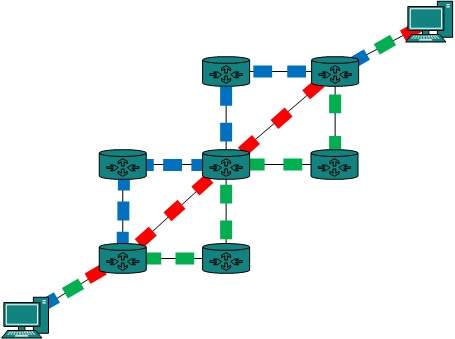 Packet switching enhances line efficiency as packets from multiple
applications can be multiplexed over the carrier. The internet uses
packet switching technique. Packet switching enables the user to
differentiate data streams based on priorities. Packets are stored and
forwarded according to their priority to provide quality of service.
Packet switching enhances line efficiency as packets from multiple
applications can be multiplexed over the carrier. The internet uses
packet switching technique. Packet switching enables the user to
differentiate data streams based on priorities. Packets are stored and
forwarded according to their priority to provide quality of service.Data link layer works between two hosts which are directly connected in some sense. This direct connection could be point to point or broadcast. Systems on broadcast network are said to be on same link. The work of data link layer tends to get more complex when it is dealing with multiple hosts on single collision domain.
Data link layer is responsible for converting data stream to signals bit by bit and to send that over the underlying hardware. At the receiving end, Data link layer picks up data from hardware which are in the form of electrical signals, assembles them in a recognizable frame format, and hands over to upper layer.
Data link layer has two sub-layers:
- Logical Link Control: It deals with protocols, flow-control, and error control
- Media Access Control: It deals with actual control of media
Functionality of Data-link Layer
Data link layer does many tasks on behalf of upper layer. These are:- Framing
Data-link layer takes packets from Network Layer and encapsulates them into Frames.Then, it sends each frame bit-by-bit on the hardware. At receiver’ end, data link layer picks up signals from hardware and assembles them into frames. - Addressing
Data-link layer provides layer-2 hardware addressing mechanism. Hardware address is assumed to be unique on the link. It is encoded into hardware at the time of manufacturing. - Synchronization
When data frames are sent on the link, both machines must be synchronized in order to transfer to take place. - Error Control
Sometimes signals may have encountered problem in transition and the bits are flipped.These errors are detected and attempted to recover actual data bits. It also provides error reporting mechanism to the sender. - Flow Control
Stations on same link may have different speed or capacity. Data-link layer ensures flow control that enables both machine to exchange data on same speed. - Multi-Access
When host on the shared link tries to transfer the data, it has a high probability of collision. Data-link layer provides mechanism such as CSMA/CD to equip capability of accessing a shared media among multiple Systems.
There are many reasons such as noise, cross-talk etc., which may help data to get corrupted during transmission. The upper layers work on some generalized view of network architecture and are not aware of actual hardware data processing.Hence, the upper layers expect error-free transmission between the systems. Most of the applications would not function expectedly if they receive erroneous data. Applications such as voice and video may not be that affected and with some errors they may still function well.
Data-link layer uses some error control mechanism to ensure that frames (data bit streams) are transmitted with certain level of accuracy. But to understand how errors is controlled, it is essential to know what types of errors may occur.
Types of Errors
There may be three types of errors:
- Single bit error
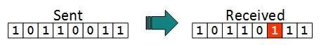 In a frame, there is only one bit, anywhere though, which is corrupt.
 - Multiple bits error
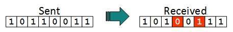 Frame is received with more than one bits in corrupted state.
 - Burst error
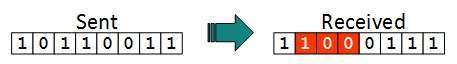 Frame contains more than1 consecutive bits corrupted.
- Error detection
- Error correction
Error Detection
Errors in the received frames are detected by means of Parity Check and Cyclic Redundancy Check (CRC). In both cases, few extra bits are sent along with actual data to confirm that bits received at other end are same as they were sent. If the counter-check at receiver’ end fails, the bits are considered corrupted.Parity Check
One extra bit is sent along with the original bits to make number of 1s either even in case of even parity, or odd in case of odd parity.The sender while creating a frame counts the number of 1s in it. For example, if even parity is used and number of 1s is even then one bit with value 0 is added. This way number of 1s remains even.If the number of 1s is odd, to make it even a bit with value 1 is added.
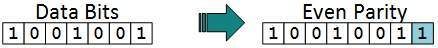 The receiver simply counts the number of 1s in a frame. If the count
of 1s is even and even parity is used, the frame is considered to be
not-corrupted and is accepted. If the count of 1s is odd and odd parity
is used, the frame is still not corrupted.
The receiver simply counts the number of 1s in a frame. If the count
of 1s is even and even parity is used, the frame is considered to be
not-corrupted and is accepted. If the count of 1s is odd and odd parity
is used, the frame is still not corrupted.If a single bit flips in transit, the receiver can detect it by counting the number of 1s. But when more than one bits are erro neous, then it is very hard for the receiver to detect the error.
Cyclic Redundancy Check (CRC)
CRC is a different approach to detect if the received frame contains valid data. This technique involves binary division of the data bits being sent. The divisor is generated using polynomials. The sender performs a division operation on the bits being sent and calculates the remainder. Before sending the actual bits, the sender adds the remainder at the end of the actual bits. Actual data bits plus the remainder is called a codeword. The sender transmits data bits as codewords.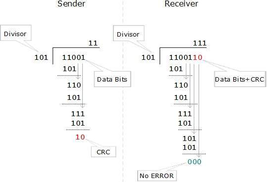 At the other end, the receiver performs division operation on
codewords using the same CRC divisor. If the remainder contains all
zeros the data bits are accepted, otherwise it is considered as there
some data corruption occurred in transit.
At the other end, the receiver performs division operation on
codewords using the same CRC divisor. If the remainder contains all
zeros the data bits are accepted, otherwise it is considered as there
some data corruption occurred in transit.Error Correction
In the digital world, error correction can be done in two ways:- Backward Error Correction When the receiver detects an error in the data received, it requests back the sender to retransmit the data unit.
- Forward Error Correction When the receiver detects some error in the data received, it executes error-correcting code, which helps it to auto-recover and to correct some kinds of errors.
To correct the error in data frame, the receiver must know exactly which bit in the frame is corrupted. To locate the bit in error, redundant bits are used as parity bits for error detection.For example, we take ASCII words (7 bits data), then there could be 8 kind of information we need: first seven bits to tell us which bit is error and one more bit to tell that there is no error.
For m data bits, r redundant bits are used. r bits can provide 2r combinations of information. In m+r bit codeword, there is possibility that the r bits themselves may get corrupted. So the number of r bits used must inform about m+r bit locations plus no-error information, i.e. m+r+1.
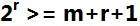
Flow Control
When a data frame (Layer-2 data) is sent from one host to another over a single medium, it is required that the sender and receiver should work at the same speed. That is, sender sends at a speed on which the receiver can process and accept the data. What if the speed (hardware/software) of the sender or receiver differs? If sender is sending too fast the receiver may be overloaded, (swamped) and data may be lost.Two types of mechanisms can be deployed to control the flow:
- Stop and Wait
This flow control mechanism forces the sender after transmitting a data frame to stop and wait until the acknowledgement of the data-frame sent is received.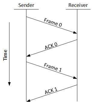
- Sliding Window
In this flow control mechanism, both sender and receiver agree on the number of data-frames after which the acknowledgement should be sent. As we learnt, stop and wait flow control mechanism wastes resources, this protocol tries to make use of underlying resources as much as possible.
Error Control
When data-frame is transmitted, there is a probability that data-frame may be lost in the transit or it is received corrupted. In both cases, the receiver does not receive the correct data-frame and sender does not know anything about any loss.In such case, both sender and receiver are equipped with some protocols which helps them to detect transit errors such as loss of data-frame. Hence, either the sender retransmits the data-frame or the receiver may request to resend the previous data-frame.Requirements for error control mechanism:
- Error detection - The sender and receiver, either both or any, must ascertain that there is some error in the transit.
- Positive ACK - When the receiver receives a correct frame, it should acknowledge it.
- Negative ACK - When the receiver receives a damaged frame or a duplicate frame, it sends a NACK back to the sender and the sender must retransmit the correct frame.
- Retransmission: The sender maintains a clock and sets a timeout period. If an acknowledgement of a data-frame previously transmitted does not arrive before the timeout the sender retransmits the frame, thinking that the frame or it’s acknowledgement is lost in transit.
Stop-and-wait ARQ
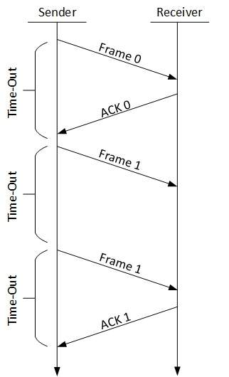 The following transition may occur in Stop-and-Wait ARQ:
- The sender maintains a timeout counter.
- When a frame is sent, the sender starts the timeout counter.
- If acknowledgement of frame comes in time, the sender transmits the next frame in queue.
- If acknowledgement does not come in time, the sender assumes that either the frame or its acknowledgement is lost in transit. Sender retransmits the frame and starts the timeout counter.
- If a negative acknowledgement is received, the sender retransmits the frame.
Go-Back-N ARQ
Stop and wait ARQ mechanism does not utilize the resources at their best.When the acknowledgement is received, the sender sits idle and does nothing. In Go-Back-N ARQ method, both sender and receiver maintain a window.
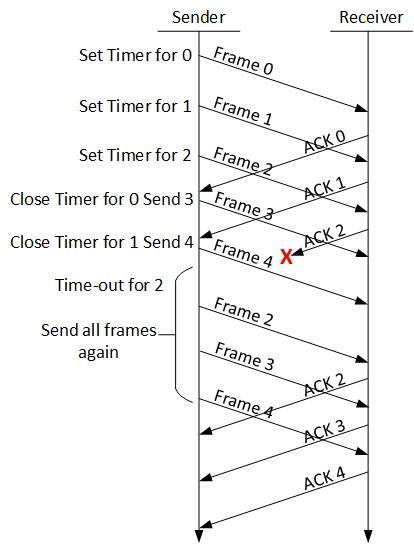 The sending-window size enables the sender to send multiple frames
without receiving the acknowledgement of the previous ones. The
receiving-window enables the receiver to receive multiple frames and
acknowledge them. The receiver keeps track of incoming frame’s sequence
number.
The sending-window size enables the sender to send multiple frames
without receiving the acknowledgement of the previous ones. The
receiving-window enables the receiver to receive multiple frames and
acknowledge them. The receiver keeps track of incoming frame’s sequence
number.
When the sender sends all the frames in window, it checks up to what sequence number it has received positive acknowledgement. If all frames are positively acknowledged, the sender sends next set of frames. If sender finds that it has received NACK or has not receive any ACK for a particular frame, it retransmits all the frames after which it does not receive any positive ACK.
Selective Repeat ARQ
In Go-back-N ARQ, it is assumed that the receiver does not have any buffer space for its window size and has to process each frame as it comes. This enforces the sender to retransmit all the frames which are not acknowledged.
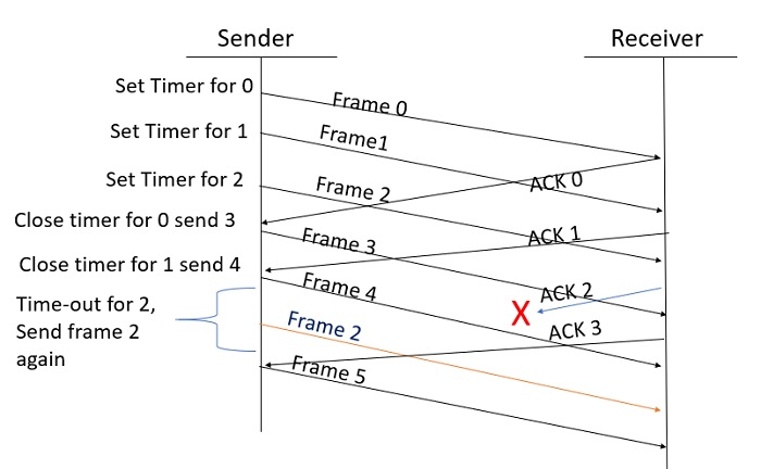 In Selective-Repeat ARQ, the receiver while keeping track of sequence
numbers, buffers the frames in memory and sends NACK for only frame
which is missing or damaged.
In Selective-Repeat ARQ, the receiver while keeping track of sequence
numbers, buffers the frames in memory and sends NACK for only frame
which is missing or damaged.
The sender in this case, sends only packet for which NACK is received .
Network layer takes the responsibility for routing packets from source to destination within or outside a subnet. Two different subnet may have different addressing schemes or non-compatible addressing types. Same with protocols, two different subnet may be operating on different protocols which are not compatible with each other. Network layer has the responsibility to route the packets from source to destination, mapping different addressing schemes and protocols.
Layer-3 Functionalities
Devices which work on Network Layer mainly focus on routing. Routing may include various tasks aimed to achieve a single goal. These can be:- Addressing devices and networks.
- Populating routing tables or static routes.
- Queuing incoming and outgoing data and then forwarding them according to quality of service constraints set for those packets.
- Internetworking between two different subnets.
- Delivering packets to destination with best efforts.
- Provides connection oriented and connection less mechanism.
Network Layer Features
With its standard functionalities, Layer 3 can provide various features as:- Quality of service management
- Load balancing and link management
- Security
- Interrelation of different protocols and subnets with different schema.
- Different logical network design over the physical network design.
- L3 VPN and tunnels can be used to provide end to end dedicated connectivity.
A network address always points to host / node / server or it can represent a whole network. Network address is always configured on network interface card and is generally mapped by system with the MAC address (hardware address or layer-2 address) of the machine for Layer-2 communication.
There are different kinds of network addresses in existence:
- IP
- IPX
- AppleTalk
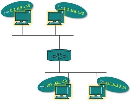 IP addressing provides mechanism to differentiate between hosts and
network. Because IP addresses are assigned in hierarchical manner, a
host always resides under a specific network.The host which needs to
communicate outside its subnet, needs to know destination network
address, where the packet/data is to be sent.
IP addressing provides mechanism to differentiate between hosts and
network. Because IP addresses are assigned in hierarchical manner, a
host always resides under a specific network.The host which needs to
communicate outside its subnet, needs to know destination network
address, where the packet/data is to be sent.Hosts in different subnet need a mechanism to locate each other. This task can be done by DNS. DNS is a server which provides Layer-3 address of remote host mapped with its domain name or FQDN. When a host acquires the Layer-3 Address (IP Address) of the remote host, it forwards all its packet to its gateway. A gateway is a router equipped with all the information which leads to route packets to the destination host.
Routers take help of routing tables, which has the following information:
- Method to reach the network
The next router on the path follows the same thing and eventually the data packet reaches its destination.
Network address can be of one of the following:
- Unicast (destined to one host)
- Multicast (destined to group)
- Broadcast (destined to all)
- Anycast (destined to nearest one)
A router is always configured with some default route. A default route tells the router where to forward a packet if there is no route found for specific destination. In case there are multiple path existing to reach the same destination, router can make decision based on the following information:
- Hop Count
- Bandwidth
- Metric
- Prefix-length
- Delay
Unicast routing
Most of the traffic on the internet and intranets known as unicast data or unicast traffic is sent with specified destination. Routing unicast data over the internet is called unicast routing. It is the simplest form of routing because the destination is already known. Hence the router just has to look up the routing table and forward the packet to next hop.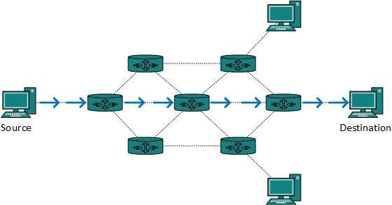
Broadcast routing
By default, the broadcast packets are not routed and forwarded by the routers on any network. Routers create broadcast domains. But it can be configured to forward broadcasts in some special cases. A broadcast message is destined to all network devices.Broadcast routing can be done in two ways (algorithm):
- A router creates a data packet and then sends it to each host one
by one. In this case, the router creates multiple copies of single
data packet with different destination addresses. All packets are sent
as unicast but because they are sent to all, it simulates as if router
is broadcasting.
This method consumes lots of bandwidth and router must destination address of each node. - Secondly, when router receives a packet that is to be
broadcasted, it simply floods those packets out of all interfaces. All
routers are configured in the same way.
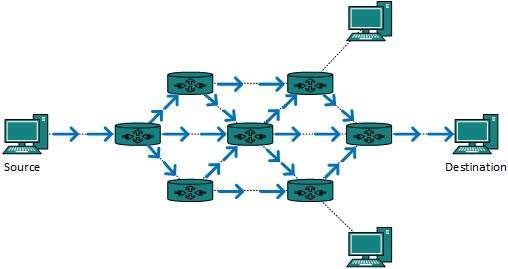 This method is easy on router's CPU but may cause the problem of duplicate packets received from peer routers.
Reverse path forwarding is a technique, in which router knows in advance about its predecessor from where it should receive broadcast. This technique is used to detect and discard duplicates.
Multicast Routing
Multicast routing is special case of broadcast routing with significance difference and challenges. In broadcast routing, packets are sent to all nodes even if they do not want it. But in Multicast routing, the data is sent to only nodes which wants to receive the packets.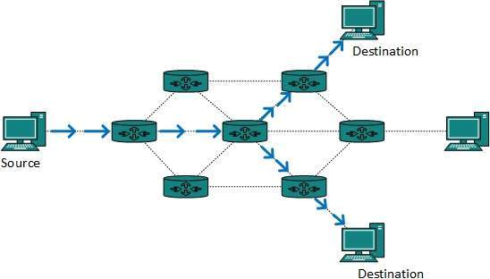 The router must know that there are nodes, which wish to receive
multicast packets (or stream) then only it should forward. Multicast
routing works spanning tree protocol to avoid looping.
The router must know that there are nodes, which wish to receive
multicast packets (or stream) then only it should forward. Multicast
routing works spanning tree protocol to avoid looping.Multicast routing also uses reverse path Forwarding technique, to detect and discard duplicates and loops.
Anycast Routing
Anycast packet forwarding is a mechanism where multiple hosts can have same logical address. When a packet destined to this logical address is received, it is sent to the host which is nearest in routing topology.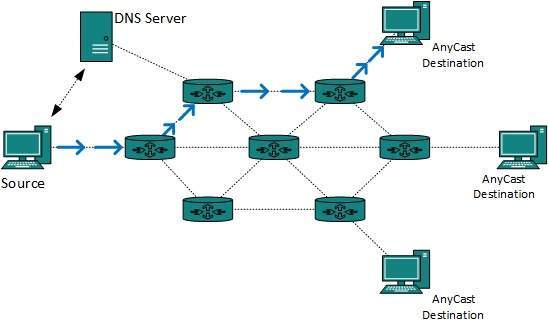 Anycast routing is done with help of DNS server. Whenever an Anycast
packet is received it is enquired with DNS to where to send it. DNS
provides the IP address which is the nearest IP configured on it.
Anycast routing is done with help of DNS server. Whenever an Anycast
packet is received it is enquired with DNS to where to send it. DNS
provides the IP address which is the nearest IP configured on it.Unicast Routing Protocols
There are two kinds of routing protocols available to route unicast packets:Distance Vector Routing Protocol
Distance Vector is simple routing protocol which takes routing decision on the number of hops between source and destination. A route with less number of hops is considered as the best route. Every router advertises its set best routes to other routers. Ultimately, all routers build up their network topology based on the advertisements of their peer routers,
For example Routing Information Protocol (RIP).Link State Routing Protocol
Link State protocol is slightly complicated protocol than Distance Vector. It takes into account the states of links of all the routers in a network. This technique helps routes build a common graph of the entire network. All routers then calculate their best path for routing purposes.for example, Open Shortest Path First (OSPF) and Intermediate System to Intermediate System (ISIS).
Multicast Routing Protocols
Unicast routing protocols use graphs while Multicast routing protocols use trees, i.e. spanning tree to avoid loops. The optimal tree is called shortest path spanning tree.- DVMRP - Distance Vector Multicast Routing Protocol
- MOSPF - Multicast Open Shortest Path First
- CBT - Core Based Tree
- PIM - Protocol independent Multicast
- PIM Dense Mode
This mode uses source-based trees. It is used in dense environment such as LAN. - PIM Sparse Mode
This mode uses shared trees. It is used in sparse environment such as WAN.
Routing Algorithms
The routing algorithms are as follows:Flooding
Flooding is simplest method packet forwarding. When a packet is received, the routers send it to all the interfaces except the one on which it was received. This creates too much burden on the network and lots of duplicate packets wandering in the network.Time to Live (TTL) can be used to avoid infinite looping of packets. There exists another approach for flooding, which is called Selective Flooding to reduce the overhead on the network. In this method, the router does not flood out on all the interfaces, but selective ones.
Shortest Path
Routing decision in networks, are mostly taken on the basis of cost between source and destination. Hop count plays major role here. Shortest path is a technique which uses various algorithms to decide a path with minimum number of hops.Common shortest path algorithms are:
- Dijkstra's algorithm
- Bellman Ford algorithm
- Floyd Warshall algorithm
Networks can be considered different based on various parameters such as, Protocol, topology, Layer-2 network and addressing scheme.
In internetworking, routers have knowledge of each other’s address and addresses beyond them. They can be statically configured go on different network or they can learn by using internetworking routing protocol.
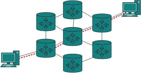 Routing protocols which are used within an organization or
administration are called Interior Gateway Protocols or IGP. RIP, OSPF
are examples of IGP. Routing between different organizations or
administrations may have Exterior Gateway Protocol, and there is only
one EGP i.e. Border Gateway Protocol.
Routing protocols which are used within an organization or
administration are called Interior Gateway Protocols or IGP. RIP, OSPF
are examples of IGP. Routing between different organizations or
administrations may have Exterior Gateway Protocol, and there is only
one EGP i.e. Border Gateway Protocol.Tunneling
If they are two geographically separate networks, which want to communicate with each other, they may deploy a dedicated line between or they have to pass their data through intermediate networks.Tunneling is a mechanism by which two or more same networks communicate with each other, by passing intermediate networking complexities. Tunneling is configured at both ends.
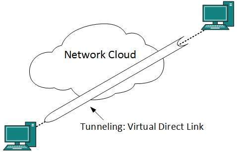 When the data enters from one end of Tunnel, it is tagged. This
tagged data is then routed inside the intermediate or transit network to
reach the other end of Tunnel. When data exists the Tunnel its tag is
removed and delivered to the other part of the network.
When the data enters from one end of Tunnel, it is tagged. This
tagged data is then routed inside the intermediate or transit network to
reach the other end of Tunnel. When data exists the Tunnel its tag is
removed and delivered to the other part of the network.Both ends seem as if they are directly connected and tagging makes data travel through transit network without any modifications.
Packet Fragmentation
Most Ethernet segments have their maximum transmission unit (MTU) fixed to 1500 bytes. A data packet can have more or less packet length depending upon the application. Devices in the transit path also have their hardware and software capabilities which tell what amount of data that device can handle and what size of packet it can process.If the data packet size is less than or equal to the size of packet the transit network can handle, it is processed neutrally. If the packet is larger, it is broken into smaller pieces and then forwarded. This is called packet fragmentation. Each fragment contains the same destination and source address and routed through transit path easily. At the receiving end it is assembled again.
If a packet with DF (don’t fragment) bit set to 1 comes to a router which can not handle the packet because of its length, the packet is dropped.
When a packet is received by a router has its MF (more fragments) bit set to 1, the router then knows that it is a fragmented packet and parts of the original packet is on the way.
If packet is fragmented too small, the overhead is increases. If the packet is fragmented too large, intermediate router may not be able to process it and it might get dropped.
Address Resolution Protocol(ARP)
While communicating, a host needs Layer-2 (MAC) address of the destination machine which belongs to the same broadcast domain or network. A MAC address is physically burnt into the Network Interface Card (NIC) of a machine and it never changes.On the other hand, IP address on the public domain is rarely changed. If the NIC is changed in case of some fault, the MAC address also changes. This way, for Layer-2 communication to take place, a mapping between the two is required.
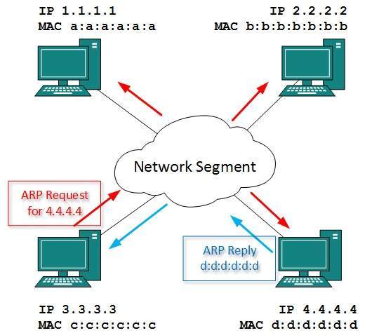 To know the MAC address of remote host on a broadcast domain, a
computer wishing to initiate communication sends out an ARP broadcast
message asking, “Who has this IP address?” Because it is a broadcast,
all hosts on the network segment (broadcast domain) receive this packet
and process it. ARP packet contains the IP address of destination host,
the sending host wishes to talk to. When a host receives an ARP packet
destined to it, it replies back with its own MAC address.
To know the MAC address of remote host on a broadcast domain, a
computer wishing to initiate communication sends out an ARP broadcast
message asking, “Who has this IP address?” Because it is a broadcast,
all hosts on the network segment (broadcast domain) receive this packet
and process it. ARP packet contains the IP address of destination host,
the sending host wishes to talk to. When a host receives an ARP packet
destined to it, it replies back with its own MAC address.Once the host gets destination MAC address, it can communicate with remote host using Layer-2 link protocol. This MAC to IP mapping is saved into ARP cache of both sending and receiving hosts. Next time, if they require to communicate, they can directly refer to their respective ARP cache.
Reverse ARP is a mechanism where host knows the MAC address of remote host but requires to know IP address to communicate.
Internet Control Message Protocol (ICMP)
ICMP is network diagnostic and error reporting protocol. ICMP belongs to IP protocol suite and uses IP as carrier protocol. After constructing ICMP packet, it is encapsulated in IP packet. Because IP itself is a best-effort non-reliable protocol, so is ICMP.Any feedback about network is sent back to the originating host. If some error in the network occurs, it is reported by means of ICMP. ICMP contains dozens of diagnostic and error reporting messages.
ICMP-echo and ICMP-echo-reply are the most commonly used ICMP messages to check the reachability of end-to-end hosts. When a host receives an ICMP-echo request, it is bound to send back an ICMP-echo-reply. If there is any problem in the transit network, the ICMP will report that problem.
Internet Protocol Version 4 (IPv4)
IPv4 is 32-bit addressing scheme used as TCP/IP host addressing mechanism. IP addressing enables every host on the TCP/IP network to be uniquely identifiable.IPv4 provides hierarchical addressing scheme which enables it to divide the network into sub-networks, each with well-defined number of hosts. IP addresses are divided into many categories:
- Class A - it uses first octet for network addresses and last three octets for host addressing
- Class B - it uses first two octets for network addresses and last two for host addressing
- Class C - it uses first three octets for network addresses and last one for host addressing
- Class D - it provides flat IP addressing scheme in contrast to hierarchical structure for above three.
- Class E - It is used as experimental.
Though IP is not reliable one; it provides ‘Best-Effort-Delivery’ mechanism.
Internet Protocol Version 6 (IPv6)
Exhaustion of IPv4 addresses gave birth to a next generation Internet Protocol version 6. IPv6 addresses its nodes with 128-bit wide address providing plenty of address space for future to be used on entire planet or beyond.IPv6 has introduced Anycast addressing but has removed the concept of broadcasting. IPv6 enables devices to self-acquire an IPv6 address and communicate within that subnet. This auto-configuration removes the dependability of Dynamic Host Configuration Protocol (DHCP) servers. This way, even if the DHCP server on that subnet is down, the hosts can communicate with each other.
IPv6 provides new feature of IPv6 mobility. Mobile IPv6 equipped machines can roam around without the need of changing their IP addresses.
IPv6 is still in transition phase and is expected to replace IPv4 completely in coming years. At present, there are few networks which are running on IPv6. There are some transition mechanisms available for IPv6 enabled networks to speak and roam around different networks easily on IPv4. These are:
- Dual stack implementation
- Tunneling
- NAT-PT
Transport layer offers peer-to-peer and end-to-end connection between two processes on remote hosts. Transport layer takes data from upper layer (i.e. Application layer) and then breaks it into smaller size segments, numbers each byte, and hands over to lower layer (Network Layer) for delivery.
Functions
- This Layer is the first one which breaks the information data, supplied by Application layer in to smaller units called segments. It numbers every byte in the segment and maintains their accounting.
- This layer ensures that data must be received in the same sequence in which it was sent.
- This layer provides end-to-end delivery of data between hosts which may or may not belong to the same subnet.
- All server processes intend to communicate over the network are equipped with well-known Transport Service Access Points (TSAPs) also known as port numbers.
End-to-End Communication
A process on one host identifies its peer host on remote network by means of TSAPs, also known as Port numbers. TSAPs are very well defined and a process which is trying to communicate with its peer knows this in advance.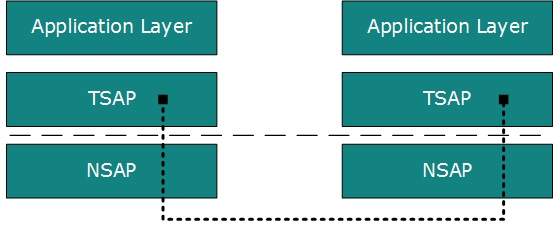 For example, when a DHCP client wants to communicate with remote DHCP
server, it always requests on port number 67. When a DNS client wants
to communicate with remote DNS server, it always requests on port number
53 (UDP).
For example, when a DHCP client wants to communicate with remote DHCP
server, it always requests on port number 67. When a DNS client wants
to communicate with remote DNS server, it always requests on port number
53 (UDP).The two main Transport layer protocols are:
- Transmission Control Protocol
It provides reliable communication between two hosts. - User Datagram Protocol
It provides unreliable communication between two hosts.
Features
- TCP is reliable protocol. That is, the receiver always sends either positive or negative acknowledgement about the data packet to the sender, so that the sender always has bright clue about whether the data packet is reached the destination or it needs to resend it.
- TCP ensures that the data reaches intended destination in the same order it was sent.
- TCP is connection oriented. TCP requires that connection between two remote points be established before sending actual data.
- TCP provides error-checking and recovery mechanism.
- TCP provides end-to-end communication.
- TCP provides flow control and quality of service.
- TCP operates in Client/Server point-to-point mode.
- TCP provides full duplex server, i.e. it can perform roles of both receiver and sender.
Header
The length of TCP header is minimum 20 bytes long and maximum 60 bytes.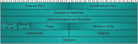
- Source Port (16-bits) - It identifies source port of the application process on the sending device.
- Destination Port (16-bits) - It identifies destination port of the application process on the receiving device.
- Sequence Number (32-bits) - Sequence number of data bytes of a segment in a session.
- Acknowledgement Number (32-bits) - When ACK flag is set, this number contains the next sequence number of the data byte expected and works as acknowledgement of the previous data received.
- Data Offset (4-bits) - This field implies both, the size of TCP header (32-bit words) and the offset of data in current packet in the whole TCP segment.
- Reserved (3-bits) - Reserved for future use and all are set zero by default.
- Flags (1-bit each)
- NS - Nonce Sum bit is used by Explicit Congestion Notification signaling process.
- CWR - When a host receives packet with ECE bit set, it sets Congestion Windows Reduced to acknowledge that ECE received.
- ECE -It has two meanings:
- If SYN bit is clear to 0, then ECE means that the IP packet has its CE (congestion experience) bit set.
- If SYN bit is set to 1, ECE means that the device is ECT capable.
- URG - It indicates that Urgent Pointer field has significant data and should be processed.
- ACK - It indicates that Acknowledgement field has significance. If ACK is cleared to 0, it indicates that packet does not contain any acknowledgement.
- PSH - When set, it is a request to the receiving station to PUSH data (as soon as it comes) to the receiving application without buffering it.
- RST - Reset flag has the following features:
- It is used to refuse an incoming connection.
- It is used to reject a segment.
- It is used to restart a connection.
- SYN - This flag is used to set up a connection between hosts.
- FIN - This flag is used to release a connection and no more data is exchanged thereafter. Because packets with SYN and FIN flags have sequence numbers, they are processed in correct order.
- Windows Size - This field is used for flow control between two stations and indicates the amount of buffer (in bytes) the receiver has allocated for a segment, i.e. how much data is the receiver expecting.
- Checksum - This field contains the checksum of Header, Data and Pseudo Headers.
- Urgent Pointer - It points to the urgent data byte if URG flag is set to 1.
- Options - It facilitates additional options which are not covered by the regular header. Option field is always described in 32-bit words. If this field contains data less than 32-bit, padding is used to cover the remaining bits to reach 32-bit boundary.
Addressing
TCP communication between two remote hosts is done by means of port numbers (TSAPs). Ports numbers can range from 0 – 65535 which are divided as:- System Ports (0 – 1023)
- User Ports ( 1024 – 49151)
- Private/Dynamic Ports (49152 – 65535)
Connection Management
TCP communication works in Server/Client model. The client initiates the connection and the server either accepts or rejects it. Three-way handshaking is used for connection management.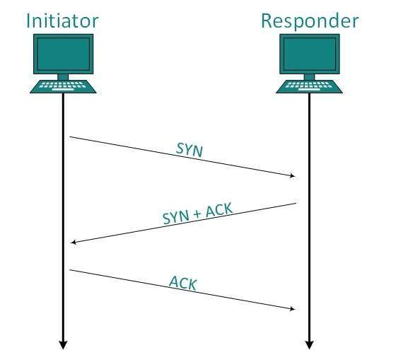
Establishment
Client initiates the connection and sends the segment with a Sequence number. Server acknowledges it back with its own Sequence number and ACK of client’s segment which is one more than client’s Sequence number. Client after receiving ACK of its segment sends an acknowledgement of Server’s response.Release
Either of server and client can send TCP segment with FIN flag set to 1. When the receiving end responds it back by ACKnowledging FIN, that direction of TCP communication is closed and connection is released.Bandwidth Management
TCP uses the concept of window size to accommodate the need of Bandwidth management. Window size tells the sender at the remote end, the number of data byte segments the receiver at this end can receive. TCP uses slow start phase by using window size 1 and increases the window size exponentially after each successful communication.For example, the client uses windows size 2 and sends 2 bytes of data. When the acknowledgement of this segment received the windows size is doubled to 4 and next sent the segment sent will be 4 data bytes long. When the acknowledgement of 4-byte data segment is received, the client sets windows size to 8 and so on.
If an acknowledgement is missed, i.e. data lost in transit network or it received NACK, then the window size is reduced to half and slow start phase starts again.
Error Control &and Flow Control
TCP uses port numbers to know what application process it needs to handover the data segment. Along with that, it uses sequence numbers to synchronize itself with the remote host. All data segments are sent and received with sequence numbers. The Sender knows which last data segment was received by the Receiver when it gets ACK. The Receiver knows about the last segment sent by the Sender by referring to the sequence number of recently received packet.If the sequence number of a segment recently received does not match with the sequence number the receiver was expecting, then it is discarded and NACK is sent back. If two segments arrive with the same sequence number, the TCP timestamp value is compared to make a decision.
Multiplexing
The technique to combine two or more data streams in one session is called Multiplexing. When a TCP client initializes a connection with Server, it always refers to a well-defined port number which indicates the application process. The client itself uses a randomly generated port number from private port number pools.Using TCP Multiplexing, a client can communicate with a number of different application process in a single session. For example, a client requests a web page which in turn contains different types of data (HTTP, SMTP, FTP etc.) the TCP session timeout is increased and the session is kept open for longer time so that the three-way handshake overhead can be avoided.
This enables the client system to receive multiple connection over single virtual connection. These virtual connections are not good for Servers if the timeout is too long.
Congestion Control
When large amount of data is fed to system which is not capable of handling it, congestion occurs. TCP controls congestion by means of Window mechanism. TCP sets a window size telling the other end how much data segment to send. TCP may use three algorithms for congestion control:- Additive increase, Multiplicative Decrease
- Slow Start
- Timeout React
Timer Management
TCP uses different types of timer to control and management various tasks:Keep-alive timer:
- This timer is used to check the integrity and validity of a connection.
- When keep-alive time expires, the host sends a probe to check if the connection still exists.
Retransmission timer:
- This timer maintains stateful session of data sent.
- If the acknowledgement of sent data does not receive within the Retransmission time, the data segment is sent again.
Persist timer:
- TCP session can be paused by either host by sending Window Size 0.
- To resume the session a host needs to send Window Size with some larger value.
- If this segment never reaches the other end, both ends may wait for each other for infinite time.
- When the Persist timer expires, the host re-sends its window size to let the other end know.
- Persist Timer helps avoid deadlocks in communication.
Timed-Wait:
- After releasing a connection, either of the hosts waits for a Timed-Wait time to terminate the connection completely.
- This is in order to make sure that the other end has received the acknowledgement of its connection termination request.
- Timed-out can be a maximum of 240 seconds (4 minutes).
Crash Recovery
TCP is very reliable protocol. It provides sequence number to each of byte sent in segment. It provides the feedback mechanism i.e. when a host receives a packet, it is bound to ACK that packet having the next sequence number expected (if it is not the last segment).When a TCP Server crashes mid-way communication and re-starts its process it sends TPDU broadcast to all its hosts. The hosts can then send the last data segment which was never unacknowledged and carry onwards.
In UDP, the receiver does not generate an acknowledgement of packet received and in turn, the sender does not wait for any acknowledgement of packet sent. This shortcoming makes this protocol unreliable as well as easier on processing.
Requirement of UDP
A question may arise, why do we need an unreliable protocol to transport the data? We deploy UDP where the acknowledgement packets share significant amount of bandwidth along with the actual data. For example, in case of video streaming, thousands of packets are forwarded towards its users. Acknowledging all the packets is troublesome and may contain huge amount of bandwidth wastage. The best delivery mechanism of underlying IP protocol ensures best efforts to deliver its packets, but even if some packets in video streaming get lost, the impact is not calamitous and can be ignored easily. Loss of few packets in video and voice traffic sometimes goes unnoticed.Features
- UDP is used when acknowledgement of data does not hold any significance.
- UDP is good protocol for data flowing in one direction.
- UDP is simple and suitable for query based communications.
- UDP is not connection oriented.
- UDP does not provide congestion control mechanism.
- UDP does not guarantee ordered delivery of data.
- UDP is stateless.
- UDP is suitable protocol for streaming applications such as VoIP, multimedia streaming.
UDP Header
UDP header is as simple as its function.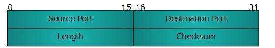 UDP header contains four main parameters:
- Source Port - This 16 bits information is used to identify the source port of the packet.
- Destination Port - This 16 bits information, is used identify application level service on destination machine.
- Length - Length field specifies the entire length of UDP packet (including header). It is 16-bits field and minimum value is 8-byte, i.e. the size of UDP header itself.
- Checksum - This field stores the checksum value generated by the sender before sending. IPv4 has this field as optional so when checksum field does not contain any value it is made 0 and all its bits are set to zero.
UDP application
Here are few applications where UDP is used to transmit data:- Domain Name Services
- Simple Network Management Protocol
- Trivial File Transfer Protocol
- Routing Information Protocol
- Kerberos
A user may or may not directly interacts with the applications. Application layer is where the actual communication is initiated and reflects. Because this layer is on the top of the layer stack, it does not serve any other layers. Application layer takes the help of Transport and all layers below it to communicate or transfer its data to the remote host.
When an application layer protocol wants to communicate with its peer application layer protocol on remote host, it hands over the data or information to the Transport layer. The transport layer does the rest with the help of all the layers below it.
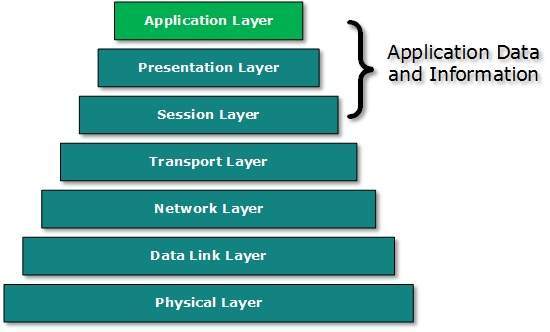 There’is an ambiguity in understanding Application Layer and its
protocol. Not every user application can be put into Application Layer.
except those applications which interact with the communication system.
For example, designing software or text-editor cannot be considered as
application layer programs.
There’is an ambiguity in understanding Application Layer and its
protocol. Not every user application can be put into Application Layer.
except those applications which interact with the communication system.
For example, designing software or text-editor cannot be considered as
application layer programs.On the other hand, when we use a Web Browser, which is actually using Hyper Text Transfer Protocol (HTTP) to interact with the network. HTTP is Application Layer protocol.
Another example is File Transfer Protocol, which helps a user to transfer text based or binary files across the network. A user can use this protocol in either GUI based software like FileZilla or CuteFTP and the same user can use FTP in Command Line mode.
Hence, irrespective of which software you use, it is the protocol which is considered at Application Layer used by that software. DNS is a protocol which helps user application protocols such as HTTP to accomplish its work.
- Peer-to-peer: Both remote processes are executing at same level and they exchange data using some shared resource.
- Client-Server: One remote process acts as a Client and requests some resource from another application process acting as Server.
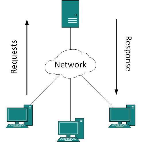 A system can act as Server and Client simultaneously. That is, one
process is acting as Server and another is acting as a client. This may
also happen that both client and server processes reside on the same
machine.
A system can act as Server and Client simultaneously. That is, one
process is acting as Server and another is acting as a client. This may
also happen that both client and server processes reside on the same
machine.Communication
Two processes in client-server model can interact in various ways:- Sockets
- Remote Procedure Calls (RPC)
Sockets
In this paradigm, the process acting as Server opens a socket using a well-known (or known by client) port and waits until some client request comes. The second process acting as a Client also opens a socket but instead of waiting for an incoming request, the client processes ‘requests first’.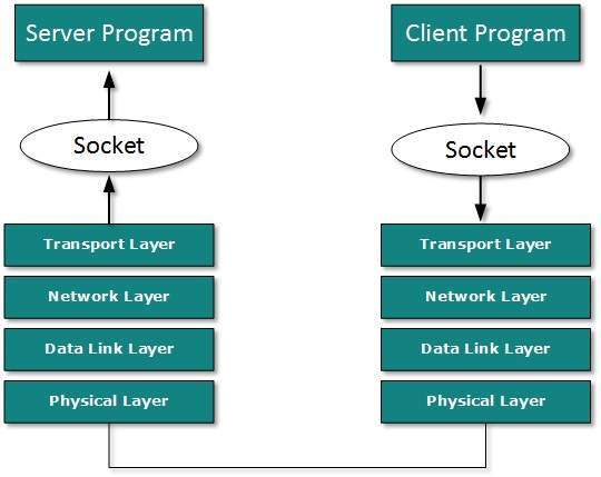 When the request is reached to server, it is served. It can either be an information sharing or resource request.
Remote Procedure Call
This is a mechanism where one process interacts with another by means of procedure calls. One process (client) calls the procedure lying on remote host. The process on remote host is said to be Server. Both processes are allocated stubs. This communication happens in the following way:- The client process calls the client stub. It passes all the parameters pertaining to program local to it.
- All parameters are then packed (marshalled) and a system call is made to send them to other side of the network.
- Kernel sends the data over the network and the other end receives it.
- The remote host passes data to the server stub where it is unmarshalled.
- The parameters are passed to the procedure and the procedure is then executed.
- The result is sent back to the client in the same manner.
- Protocols which are used by users.For email for example, eMail.
- Protocols which help and support protocols used by users.For example DNS.
Domain Name System
The Domain Name System (DNS) works on Client Server model. It uses UDP protocol for transport layer communication. DNS uses hierarchical domain based naming scheme. The DNS server is configured with Fully Qualified Domain Names (FQDN) and email addresses mapped with their respective Internet Protocol addresses.A DNS server is requested with FQDN and it responds back with the IP address mapped with it. DNS uses UDP port 53.
Simple Mail Transfer Protocol
The Simple Mail Transfer Protocol (SMTP) is used to transfer electronic mail from one user to another. This task is done by means of email client software (User Agents) the user is using. User Agents help the user to type and format the email and store it until internet is available. When an email is submitted to send, the sending process is handled by Message Transfer Agent which is normally comes inbuilt in email client software.Message Transfer Agent uses SMTP to forward the email to another Message Transfer Agent (Server side). While SMTP is used by end user to only send the emails, the Servers normally use SMTP to send as well as receive emails. SMTP uses TCP port number 25 and 587.
Client software uses Internet Message Access Protocol (IMAP) or POP protocols to receive emails.
File Transfer Protocol
The File Transfer Protocol (FTP) is the most widely used protocol for file transfer over the network. FTP uses TCP/IP for communication and it works on TCP port 21. FTP works on Client/Server Model where a client requests file from Server and server sends requested resource back to the client.FTP uses out-of-band controlling i.e. FTP uses TCP port 20 for exchanging controlling information and the actual data is sent over TCP port 21.
The client requests the server for a file. When the server receives a request for a file, it opens a TCP connection for the client and transfers the file. After the transfer is complete, the server closes the connection. For a second file, client requests again and the server reopens a new TCP connection.
Post Office Protocol (POP)
The Post Office Protocol version 3 (POP 3) is a simple mail retrieval protocol used by User Agents (client email software) to retrieve mails from mail server.When a client needs to retrieve mails from server, it opens a connection with the server on TCP port 110. User can then access his mails and download them to the local computer. POP3 works in two modes. The most common mode the delete mode, is to delete the emails from remote server after they are downloaded to local machines. The second mode, the keep mode, does not delete the email from mail server and gives the user an option to access mails later on mail server.
Hyper Text Transfer Protocol (HTTP)
The Hyper Text Transfer Protocol (HTTP) is the foundation of World Wide Web. Hypertext is well organized documentation system which uses hyperlinks to link the pages in the text documents. HTTP works on client server model. When a user wants to access any HTTP page on the internet, the client machine at user end initiates a TCP connection to server on port 80. When the server accepts the client request, the client is authorized to access web pages.To access the web pages, a client normally uses web browsers, who are responsible for initiating, maintaining, and closing TCP connections. HTTP is a stateless protocol, which means the Server maintains no information about earlier requests by clients.
HTTP versions
- HTTP 1.0 uses non persistent HTTP. At most one object can be sent over a single TCP connection.
- HTTP 1.1 uses persistent HTTP. In this version, multiple objects can be sent over a single TCP connection.
Directory Services
These services are mapping between name and its value, which can be variable value or fixed. This software system helps to store the information, organize it, and provides various means of accessing it.- Accounting
In an organization, a number of users have their user names and passwords mapped to them. Directory Services provide means of storing this information in cryptic form and make available when requested. - Authentication and Authorization
User credentials are checked to authenticate a user at the time of login and/or periodically. User accounts can be set into hierarchical structure and their access to resources can be controlled using authorization schemes. - Domain Name Services
DNS is widely used and one of the essential services on which internet works. This system maps IP addresses to domain names, which are easier to remember and recall than IP addresses. Because network operates with the help of IP addresses and humans tend to remember website names, the DNS provides website’s IP address which is mapped to its name from the back-end on the request of a website name from the user.
File Services
File services include sharing and transferring files over the network.- File Sharing
One of the reason which gave birth to networking was file sharing. File sharing enables its users to share their data with other users. User can upload the file to a specific server, which is accessible by all intended users. As an alternative, user can make its file shared on its own computer and provides access to intended users. - File Transfer
This is an activity to copy or move file from one computer to another computer or to multiple computers, with help of underlying network. Network enables its user to locate other users in the network and transfers files.
Communication Services
- Email
Electronic mail is a communication method and something a computer user cannot work without. This is the basis of today’s internet features. Email system has one or more email servers. All its users are provided with unique IDs. When a user sends email to other user, it is actually transferred between users with help of email server. - Social Networking
Recent technologies have made technical life social. The computer savvy peoples, can find other known peoples or friends, can connect with them, and can share thoughts, pictures, and videos. - Internet Chat
Internet chat provides instant text transfer services between two hosts. Two or more people can communicate with each other using text based Internet Relay Chat services. These days, voice chat and video chat are very common. - Discussion Boards
Discussion boards provide a mechanism to connect multiple peoples with same interests.It enables the users to put queries, questions, suggestions etc. which can be seen by all other users. Other may respond as well. - Remote Access
This service enables user to access the data residing on the remote computer. This feature is known as Remote desktop. This can be done via some remote device, e.g. mobile phone or home computer.
Application Services
These are nothing but providing network based services to the users such as web services, database managing, and resource sharing.- Resource Sharing
To use resources efficiently and economically, network provides a mean to share them. This may include Servers, Printers, and Storage Media etc. - Databases
This application service is one of the most important services. It stores data and information, processes it, and enables the users to retrieve it efficiently by using queries. Databases help organizations to make decisions based on statistics. - Web Services
World Wide Web has become the synonym for internet.It is used to connect to the internet, and access files and information services provided by the internet servers.
Data Communication Overview
A system of interconnected computers and computerized peripherals such as printers is called computer network. This interconnection among computers facilitates information sharing among them. Computers may connect to each other by either wired or wireless media.Classification of Computer Networks
Computer networks are classified based on various factors.They includes:- Geographical span
- Inter-connectivity
- Administration
- Architecture
Geographical Span
Geographically a network can be seen in one of the following categories:- It may be spanned across your table, among Bluetooth enabled devices,. Ranging not more than few meters.
- It may be spanned across a whole building, including intermediate devices to connect all floors.
- It may be spanned across a whole city.
- It may be spanned across multiple cities or provinces.
- It may be one network covering whole world.
Inter-Connectivity
Components of a network can be connected to each other differently in some fashion. By connectedness we mean either logically , physically , or both ways.- Every single device can be connected to every other device on network, making the network mesh.
- All devices can be connected to a single medium but geographically disconnected, created bus like structure.
- Each device is connected to its left and right peers only, creating linear structure.
- All devices connected together with a single device, creating star like structure.
- All devices connected arbitrarily using all previous ways to connect each other, resulting in a hybrid structure.
Administration
From an administrator’s point of view, a network can be private network which belongs a single autonomous system and cannot be accessed outside its physical or logical domain.A network can be public which is accessed by all.Network Architecture
- Computer networks can be discriminated into various types such as
Client-Server,peer-to-peer or hybrid, depending upon its architecture.
- There can be one or more systems acting as Server. Other being Client, requests the Server to serve requests.Server takes and processes request on behalf of Clients.
- Two systems can be connected Point-to-Point, or in back-to-back fashion. They both reside at the same level and called peers.
- There can be hybrid network which involves network architecture of both the above types.
Network Applications
Computer systems and peripherals are connected to form a network.They provide numerous advantages:- Resource sharing such as printers and storage devices
- Exchange of information by means of e-Mails and FTP
- Information sharing by using Web or Internet
- Interaction with other users using dynamic web pages
- IP phones
- Video conferences
- Parallel computing
- Instant messaging
Computer Network Types
Generally, networks are distinguished based on their geographical span. A network can be as small as distance between your mobile phone and its Bluetooth headphone and as large as the internet itself, covering the whole geographical world,Personal Area Network
A Personal Area Network (PAN) is smallest network which is very personal to a user. This may include Bluetooth enabled devices or infra-red enabled devices. PAN has connectivity range up to 10 meters. PAN may include wireless computer keyboard and mouse, Bluetooth enabled headphones, wireless printers and TV remotes.
For example, Piconet is Bluetooth-enabled Personal Area Network which
may contain up to 8 devices connected together in a master-slave
fashion.Local Area Network
A computer network spanned inside a building and operated under single administrative system is generally termed as Local Area Network (LAN). Usually,LAN covers an organization’ offices, schools, colleges or universities. Number of systems connected in LAN may vary from as least as two to as much as 16 million.LAN provides a useful way of sharing the resources between end users.The resources such as printers, file servers, scanners, and internet are easily sharable among computers.
LANs are composed of inexpensive networking and routing equipment.
It may contains local servers serving file storage and other locally
shared applications. It mostly operates on private IP addresses and
does not involve heavy routing. LAN works under its own local domain
and controlled centrally.LAN uses either Ethernet or Token-ring technology. Ethernet is most widely employed LAN technology and uses Star topology, while Token-ring is rarely seen.
LAN can be wired,wireless, or in both forms at once.
Metropolitan Area Network
The Metropolitan Area Network (MAN) generally expands throughout a city such as cable TV network. It can be in the form of Ethernet,Token-ring, ATM, or Fiber Distributed Data Interface (FDDI).Metro Ethernet is a service which is provided by ISPs. This service enables its users to expand their Local Area Networks. For example, MAN can help an organization to connect all of its offices in a city.
Backbone of MAN is high-capacity and high-speed fiber optics. MAN
works in between Local Area Network and Wide Area Network. MAN provides
uplink for LANs to WANs or internet.Wide Area Network
As the name suggests,the Wide Area Network (WAN) covers a wide area which may span across provinces and even a whole country. Generally, telecommunication networks are Wide Area Network. These networks provide connectivity to MANs and LANs. Since they are equipped with very high speed backbone, WANs use very expensive network equipment.
WAN may use advanced technologies such as Asynchronous Transfer Mode
(ATM), Frame Relay, and Synchronous Optical Network (SONET). WAN may be
managed by multiple administration.Internetwork
A network of networks is called an internetwork, or simply the internet. It is the largest network in existence on this planet.The internet hugely connects all WANs and it can have connection to LANs and Home networks. Internet uses TCP/IP protocol suite and uses IP as its addressing protocol. Present day, Internet is widely implemented using IPv4. Because of shortage of address spaces, it is gradually migrating from IPv4 to IPv6.Internet enables its users to share and access enormous amount of information worldwide. It uses WWW, FTP, email services, audio and video streaming etc. At huge level, internet works on Client-Server model.
Internet uses very high speed backbone of fiber optics. To inter-connect various continents, fibers are laid under sea known to us as submarine communication cable.
Internet is widely deployed on World Wide Web services using HTML linked pages and is accessible by client software known as Web Browsers. When a user requests a page using some web browser located on some Web Server anywhere in the world, the Web Server responds with the proper HTML page. The communication delay is very low.
Internet is serving many proposes and is involved in many aspects of life. Some of them are:
- Web sites
- Instant Messaging
- Blogging
- Social Media
- Marketing
- Networking
- Resource Sharing
- Audio and Video Streaming
Data communications refers to the transmission of this digital data between two or more computers and a computer network or data network is a telecommunications network that allows computers to exchange data. The physical connection between networked computing devices is established using either cable media or wireless media. The best-known computer network is the Internet.
This tutorial should teach you basics of Data Communication and Computer Network (DCN) and will also take you through various advance concepts related to Data Communication and Computer Network.
XO___XO SAW ADA ( ADDRESS DATA ACCUMULATION )
Route analysis concept for Real Accumulation Adresss and Data
Solving a route
analysis can mean finding the quickest, shortest, or even the most
scenic route, depending on the impedance you choose to solve for. If the
impedance is time, then the best route is the quickest route. If the
impedance is a time attribute with live or historical traffic, then the
best route is the quickest route for a given time of day and date.
Hence, the best route can be defined as the route that has the lowest
impedance, or least cost, where the impedance is chosen by you. Any cost
attribute can be used as the impedance when determining the best route.

This shows the route of the quickest path for someone to drive from point A to point B.
Route analysis
ArcMap 10.6
|
Available with Network Analyst license.
Solving a route
analysis can mean finding the quickest, shortest, or even the most
scenic route, depending on the impedance you choose to solve for. If the
impedance is time, then the best route is the quickest route. If the
impedance is a time attribute with live or historical traffic, then the
best route is the quickest route for a given time of day and date.
Hence, the best route can be defined as the route that has the lowest
impedance, or least cost, where the impedance is chosen by you. Any cost
attribute can be used as the impedance when determining the best route.
You
can accumulate any number of impedance attributes in a route analysis,
but accumulated attributes don't play a role in computing the path
along the network. For example, if you choose a time cost attribute as
the impedance attribute and want to accumulate a distance cost
attribute, only the time cost attribute is used to optimize the
solution. The total distance is accumulated and reported, but the path
isn't calculated from distance in this example.
Finding the best route through a series of stops follows the same workflow as other network analyses Route analysis layer
The route analysis layer stores all the inputs, parameters, and results of a route analysis.
Creating a route analysis layer
You can create a route analysis layer from the Network Analyst toolbar by clicking Network Analyst > New Route.

When you create a new route analysis layer, it appears in the Network Analyst window along with its five network analysis classes—Stops, Routes, Point Barriers, Line Barriers, and Polygon Barriers.
The route analysis layer also appears in the Table Of Contents
as a composite layer named Route (or, if a route with the same name
already exists in the map document, Route 1, Route 2, and so on). There
are five feature layers—Stops, Routes, Point Barriers, Line Barriers,
and Polygon Barriers. Each of the five feature layers has default
symbology that can be modified on its Layer Properties dialog box.
Route analysis classes
The route analysis layer is composed of five network analysis classes.
An overview of each class and descriptions of their properties are provided in the following sections.
Stops class
This
network analysis class stores the network locations that are used as
stops in a route analysis. The Stops layer has four default symbols:
located stops, unlocated stops, stops with errors, and stops with time
violations. You can modify the symbology for the Stops layer in the Layer Properties dialog box, where there is a custom symbology category for stops, Network Analyst > Sequenced Points.

When
a new route analysis layer is created, the Stops class is empty. It is
populated only when network locations are added to it. A minimum of two
stops is necessary to create a route.
Stop properties
Some
of the stop properties are only available when a start time is defined
or time windows are enabled, both of which are parameters on the Analysis Settings tab of the Route analysis layer's Layer Properties dialog box.
Input fields of stops
| Input field | Description |
|---|---|
ObjectID
|
The system-managed ID field.
|
Shape
|
The geometry field indicating the geographic location of the network analysis object.
|
Name
|
The name of the network analysis object.
A name, which you can edit, is assigned automatically when the stop is added to the map.
|
RouteName
|
This represents the name of the route to which the stop belongs. By
using this property, stops within one route analysis layer can be
assigned to multiple routes.
|
TimeWindowStart
|
This property stores the earliest time the network location can be visited.
If TimeWindowStart
is set to 10:00 AM and the route arrives at the stop at 9:50 AM, there
is a wait time of 10 minutes that is added to the total time.
If
the network dataset has a time-zone attribute, the time-of-day fields
refer to the same time zone as the edge on which the stop is located.
This property is only available when time windows are enabled on the network analysis layer.
|
TimeWindowEnd
|
This property stores the latest time the network location can be visited.
Together, the TimeWindowStart and TimeWindowEnd properties make up the time window within which a route can visit the network location.
If a location has a TimeWindowEnd
value of 11:00 AM, and the earliest a route can reach the stop is 11:25
AM, a violation of 25 minutes is noted. Additionally, the stop is
symbolized to display that it has a time window violation.
If
the network dataset has a time-zone attribute, the time-of-day fields
refer to the same time zone as the edge on which the stop is located.
This property is only available when time windows are enabled on the network analysis layer.
|
Attr_[Impedance]
(for instance, Attr_Minutes, where Minutes is the impedance for the network)
|
This property specifies how much time will be spent at the network
location when the route visits it; that is, it stores the impedance
value for the network location. A zero or null value indicates the
network location requires no service time.
For
example, if you are finding the best route through three stops using
Drivetime as impedance, the property Attr_Drivetime can be used to store
the amount of time you expect to spend at each stop. If you start from
Stop 1, reach Stop 2 in 10 minutes, spend 10 minutes at Stop 2, and
reach Stop 3 in another 10 minutes, the total time to reach Stop 3 is
displayed as 30 minutes (10 + 10 + 10), even though there is only 20
minutes of traveling to reach Stop 3.
|
Network location fields
|
Together, these four properties describe the point on the network where the object is located.
|
CurbApproach
|
The
CurbApproach property specifies the direction a vehicle may arrive at
and depart from the network location. There are four choices (their
coded values are shown in parentheses):
|
LocationType
|
This property describes the stop type.
|
Input/output fields of stops
| Input/Output field | Description |
|---|---|
Sequence
|
As
an input field, this number represents the order in which the stops
should be visited. Within a route, the sequence number should be greater
than 0 but not greater than the maximum number of stops. Also, the
sequence number should not be duplicated. If the analysis layer
parameter Reorder Stops To Find Optimal Route is not checked, the resulting route visits the stops in the sequence specified.
If
the stops are allowed to be reordered by the solver, the optimal
sequence is discovered, and Sequence is updated during the solve
process.
The recommended way to change the sequence value is by dragging stops above or below other stops in the Network Analyst window.
|
Status
|
This field is constrained by a domain of values, which are listed below (their coded values are shown in parentheses).
After a solve operation, the status can be modified using one of the following status values:
If time windows are used and the route arrives early or late, the value changes to Time window violation (6).
|
Output fields of stops
| Output field | Description |
|---|---|
ArriveCurbApproach
|
Indicates which side of the vehicle the curb is on when the vehicle
approaches the network location. If the network location's CurbApproach
value is set to Right side of vehicle, the ArriveCurbApproach after
solving is Right side of vehicle. However, if the CurbApproach value is
set to Either side of vehicle or No U-Turn, the ArriveCurbApproach could
be on the right or left side depending on which produces the overall
shortest path.
|
DepartCurbApproach
|
Indicates which side of the vehicle the curb is on when the vehicle
departs the network location. If the network location's CurbApproach
value is set to Right side of vehicle, the DepartCurbApproach after
solving is Right side of vehicle. However, if the CurbApproach value is
set to Either side of vehicle or No U-Turn, the DepartCurbApproach could
be on the right or left side depending on which produces the overall
shortest path.
|
Cumul_[Impedance]
(for instance, Cumul_Minutes, where Minutes is the impedance for the network)
|
This property is the total impedance it takes to reach the stop. This
includes the impedance incurred in traveling to the stop, the impedance
of the stop, and the impedances of all the previous stops.
In
the example given for the input attribute, Attr_[Impedance], the
Cumul_Drivetime for Stop 2 would be 20 minutes (10 minutes travel time +
10 minutes spent at Stop 2), and the Cumul_Drivetime for Stop 3 would
be 30 minutes (20 minutes Cumul_Drivetime for Stop 2, plus 10 minutes
travel time from Stop 2 to Stop 3).
|
Wait_[Impedance]
(for instance, Wait_Minutes, where Minutes is the impedance for the network)
|
This property stores the time spent waiting for the time window to open (TimeWindowStart) when the route arrives early.
This property is only available when time windows are enabled on the network analysis layer.
|
CumulWait_[Impedance]
(for instance, CumulWait_Minutes, where Minutes is the impedance for the network)
|
This property stores a sum of how much time has been spent waiting for
time windows to open (TimeWindowStart). It includes the time from the
current stop and all previous stops visited by the route.
This property is only available when time windows are enabled on the network analysis layer.
|
Violation_[Impedance]
|
This property is a measure of how late the route arrived after the time
window closed (TimeWindowEnd). Specifically, it stores the amount of
time between the end of the time window and the arrival of the route.
This property is only available when time windows are enabled on the network analysis layer.
|
CumulViolation_[Impedance]
|
This property stores the cumulative violation time
(Violation_[Impedance]) from the current stop and all previous stops
visited by the route.
This property is only available when time windows are enabled on the network analysis layer.
|
ArriveTime
|
The date and time value indicating the arrival time at the stop.
When
using traffic data that covers multiple time zones, the time zone for
this time-of-day value is taken from the network element on which the
order is located.
|
DepartTime
|
The date and time value indicating the departure time from the stop.
When
using traffic data that covers multiple time zones, the time zone for
this time-of-day value is taken from the network element on which the
order is located.
|
ArriveTimeUTC
|
The date and time value indicating the arrival time in Coordinated Universal Time (UTC).
|
DepartTimeUTC
|
The date and time value indicating the departure time in Coordinated Universal Time (UTC).
|
Routes class
The
Routes class stores the resulting route, or routes, from the analysis.
As with other feature layers, its symbology can be accessed and altered
from its Layer Properties dialog box.
The Routes
class is an output-only class; it is empty until the analysis is
complete. Once the best route is found, it is displayed in the Network Analyst window.
Route properties
Output fields of routes
| Output field | Description |
|---|---|
ObjectID
|
The system-managed ID field.
|
Name
|
The name for the route is assigned automatically when the route layer
is solved, either by reading the value from the RouteName property of
the Stops class or, if that value is null, by integrating the name of
the first stop in the route and the name of the last stop, for example,
Graphic Pick 1 – Graphic Pick 8. You can rename the route in the Network Analyst window.
|
FirstStopID
|
The ObjectID of the route's first stop.
|
LastStopID
|
The ObjectID of the route's last stop.
|
StopCount
|
The number of stops visited by the route.
|
Total_[Impedance]
(for instance, Total_Minutes, where Minutes is the impedance for the network)
|
The total impedance from the beginning of the first stop to the end of
the last stop. The total travel impedance and the Attr_[Impedance] of
the visited stops are included in this value.
|
TotalWait_[Impedance]
(for example, TotalWait_Minutes, where Minutes is the impedance of the network)
|
This property stores the route's overall wait time, which is the time spent at stops waiting for time windows to open.
This property is only available when time windows are enabled on the network analysis layer.
|
TotalViolation_[Impedance]
(for example, TotalViolation_Minutes, where Minutes is the impedance of the network)
|
This
property stores the route's overall violation time at stops. Violation
time is added when the route arrives at a stop after the time window has
ended; it is the difference between the ArriveTime and TimeWindowEnd.
This property is only available when time windows are enabled on the network analysis layer.
|
StartTime
|
The time the route begins.
|
EndTime
|
The time the route is complete.
|
StartTimeUTC
|
The start time of the route in UTC.
|
EndTimeUTC
|
The end time of the route in UTC.
|
Point, line, and polygon barriers
Barriers
serve to temporarily restrict, add impedance to, and scale impedance on
parts of the network. When a new network analysis layer is created, the
barrier classes are empty. They are populated only when you add objects
into them—but adding barriers is not required.
Barriers are available in all network analysis layers; therefore, they are described in a separate topic.
Route analysis parameters
Analysis parameters are set on the Layer Properties dialog box for the analysis layer. The dialog box can be accessed in different ways:
Analysis Settings tab
The following subsections list parameters that you can set on the analysis layer. They are found on the Analysis Settings tab of the analysis layer's Layer Properties dialog box.

Impedance
Any cost attribute can be chosen as the impedance, which is minimized
while determining the best route. For instance, choosing the Minutes
attribute results in the quickest route.
Restrictions
You
can choose which restriction attributes should be respected while
solving the analysis. In most cases, restrictions cause roads to be
prohibited, but they can also cause them to be avoided or preferred. A
restriction attribute, such as Oneway, should be used when finding
solutions for vehicles that must obey one-way streets (for instance,
nonemergency vehicles). Other common restriction attributes include
height or weight limits that prohibit some vehicles from traversing
certain roads or bridges; hazardous materials restrictions that hazmat
drivers need to completely bypass or at least try to avoid; and
designated truck routes that truck drivers should try to follow. You can
choose which restriction attributes should be respected while solving
the analysis. (You can further specify whether the elements that use the
restriction should be prohibited, avoided, or preferred in the Attribute Parameters tab.)
Use Start Time
Use Start Time, in conjunction with the Time of Day and Specific Date or Day of Week
properties, lets you specify when the route will begin from the first
stop. Moreover, if you specify a time-only value in any of the date/time
properties for the route analysis, such as the time window properties,
the date is assumed to be the date you set for Specific Date or Day of Week.
Note
that specifying a start time doesn't require traffic data. However, if
the network dataset includes traffic data, the results of the analysis
are more accurate. That is, the results are calculated for the start
date and time that you set. For example, during rush hour, the route
could take longer than during off-peak hours. Furthermore, the best path
could change depending on traffic conditions at that time.
The
route feature or features that are output by the solver have StartTime
and EndTime properties when a time-based impedance is used with a start
time. The StartTime value will match the value that you enter in the Use Start Time settings of the route analysis layer. The EndTime will be calculated from the start time and the duration of the route. The Directions window will display the start and end times when directions are generated.
Stops
in a route analysis have ArriveTime and DepartTime properties when a
time-based impedance is used with a start time. If you also choose to
display the Time of day column on the Directions Options dialog box, the arrive and depart times at stops will appear in the Directions window. In fact, all directives in the Directions window will display a time of day.
Time of Day
The value you enter here represents the time you want the route, or routes, to begin. The default value for Time of Day is 8:00 AM.
The time must be associated with a date. You can choose between entering a calendar day (Specific Date) or a floating day (Day of Week).
Specific Date
For a calendar date, you provide the day, month, and year that the Time of Day value is associated with.
Day of Week
For a floating day, you can choose Today or any day of the week (Sunday through Saturday)
relative to the current date. Floating days enable you to configure an
analysis layer that can be reused, without having to remember to change
the date.
Floating
days are especially beneficial when used with traffic data, since
traffic changes from minute to minute and day to day. For example, if
you calculate the same routes each day and need accurate times or the
best routes given traffic conditions, you can choose the Day of Week and Today
settings. The solver will generate results based on the traffic for the
current day, which is determined by your computer's operating system.
If you return the next day—for instance, May 5—to update the routes for
that day, you can re-solve the same analysis layer. The solution will
automatically be based on the traffic for May 5 since Day of Week was set to Today.
Likewise, when you choose Monday for the Day of Week
property, and then solve, the solution will be based on the traffic
forecast for the next Monday. However, if today is Monday, the solution
uses today's traffic data. You can solve up to six days ahead relative
to the current day.
Using a start time with traffic data and time zones
If
you use traffic data, the start time refers to the time zone of the
edge or junction on which the first stop is located. There is one case
in which this causes a solve to fail because the time zone can't be
determined beforehand. That situation is created when your stops are
located across multiple time zones, and you check Reorder Stops To Find Optimal Route without preserving the first stop. You can avoid this failure by preassigning the first stop.
Use Time Windows
If
a stop can be visited only during a particular time of day, its time
window can be stored in the TimeWindowStart and TimeWindowEnd properties
of the network location (stop). This check box enables or disables the
usage of those time windows. If time windows are enabled, the route will
be modified such that it honors the time windows. If the route is
unable to honor some time windows, the affected stops will be symbolized
as time-window violations.
Reorder Stops To Find Optimal Route
By default, a route traverses stops in the order you define. However, you can possibly shorten the route further by letting Network Analyst
find the best order. It will account for a variety of variables, such
as time windows. Another option is to preserve the origin and
destination while allowing Network Analyst to reorder the intermediary stops.
When you check this property, the route analysis changes from a shortest-path problem to a traveling salesperson problem (TSP).
U-turns at Junctions
Network Analyst can allow U-turns everywhere, nowhere, only at dead
ends (or culs-de-sac), or only at intersections and dead ends. Allowing
U-turns implies the vehicle can turn around at a junction and double
back on the same street.
Output Shape Type
The route features that are output by the analysis can be represented in one of four ways.
- True Shape gives the exact shape of the resulting route.

- True Shape with Measures
gives the exact shape of the resulting route. Furthermore, the output
includes route measurements for linear referencing. The measurements
increase from the first stop and record the cumulative impedance.
- Straight Line results in a single, straight line between the stops.

- When the output shape type is set to None, no shape is returned.
Use Hierarchy
If
the network dataset has a hierarchy attribute, you can use the
hierarchy during the analysis. Using a hierarchy results in the solver
preferring higher-order edges to lower-order edges. Hierarchical solves
are faster, and they can be used to simulate the driver preference of
traveling on freeways instead of local roads—even if that means a
longer trip. Not using a hierarchy, however, yields an exact route for
the network dataset.
Ignore Invalid Locations
This property allows you to ignore invalid network locations and solve
the analysis layer from valid network locations only. If this option is
not checked and you have unlocated network locations, the solve may
fail. In either case, the invalid locations are ignored in the analysis.
Directions
With the Directions
properties, you can set the units for displaying distance and,
optionally, time (if you have a time attribute). Additionally, you can
choose to open directions automatically after the generation of a route.
(If you choose not to display directions automatically, you can click
the Directions Window button  on the Network Analyst toolbar to display directions.)
on the Network Analyst toolbar to display directions.)Accumulation tab
Under the Accumulation
tab, you can choose cost attributes from the network dataset to be
accumulated on the route objects. These accumulation attributes are
purely for reference; the solver only uses the cost attribute specified
by the analysis layer's Impedance parameter to calculate the route.
For
each cost attribute that is accumulated, a Total_[Impedance] property
is added to the routes that are output by the solver, where [Impedance]
is replaced with the name of the accumulated impedance attribute.
Assume
you set the impedance attribute to Minutes because you want to find a
route that minimizes travel time. Even though you're solving using
travel time, you would also like to know the length of the quickest
route. Suppose you have another cost attribute, Miles, that you check on
in the Accumulation tab. After solving, the output route features will
have properties named Total_Minutes and Total_Miles.
Conversely,
you can find the shortest route and accumulate travel time to determine
when the route will arrive at its stops and how long it will take to
complete the trip. If you have a traffic-enabled network dataset, you
can even find this information for a specific time of day and account
for variable traffic speeds. To do this, choose a distance-based cost
attribute for the impedance of the analysis layer, use a start time, and
accumulate a time-dependent cost attribute.
The Network Locations tab
The parameters on the Network Locations tab are used to find network locations and set values for their properties.
Directions
Directions can be displayed in ArcMap after the generation of a route in route analysis.
To display directions, on the Network Analyst toolbar, click the Directions Window button .
.- The Directions Window displays turn-by-turn directions and maps with the impedance.
- If the impedance is set to time, the Directions Window displays the time taken for each segment of the route. Additionally, the Directions Window can display the length of each segment.
- If the route supports time windows, the Directions Window displays the Attr_[time] and Wait_[time] attributes. However, the Violation_[time] and Attr_[length] attributes are not supported.
XO___XO SAW XX FOR ADA
How Flow Accumulation works
The Flow Accumulation
tool calculates accumulated flow as the accumulated weight of all cells
flowing into each downslope cell in the output raster. If no weight
raster is provided, a weight of 1 is applied to each cell, and the value
of cells in the output raster is the number of cells that flow into
each cell.
In the
graphic below, the top left image shows the direction of travel from
each cell and the top right the number of cells that flow into each
cell.

Cells
with a high flow accumulation are areas of concentrated flow and may be
used to identify stream channels. This is discussed in Identifying stream networks. Cells with a flow accumulation of 0 are local topographic highs and may be used to identify ridges.
Example
A sample usage of the Flow Accumulation
tool with an input weight raster might be to determine how much rain
has fallen within a given watershed. In such a case, the weight raster
may be a continuous raster representing average rainfall during a given
storm. The output from the tool would then represent the amount of rain
that would flow through each cell, assuming that all rain became runoff
and there was no interception, evapotranspiration, or loss to
groundwater. This could also be viewed as the amount of rain that fell
on the surface, upslope from each cell.
The results of Flow Accumulation can be used to create a stream network by applying a threshold value to select cells with a high accumulated flow.
For
example, the procedure to create a raster where the value 1 represents
the stream network on a background of NoData could use one of the
following:
- Perform a conditional operation with the Con tool with the following settings:
- Input conditional raster : FlowaccExpression : Value > 100Input true raster or constant : 1
-
- Alternatively, run the Set Null tool with the following settings:
- Input conditional raster: : FlowaccExpression: : Value <= 100Input false raster or constant: : 1
-
In
both examples, all cells that have more than 100 cells flowing into
them are assigned 1; all other cells are assigned NoData. For future
processing, it is important that the stream network, a set of raster
linear features, be represented as values on a background of NoData.
This
method of deriving accumulated flow from a DEM is presented in Jenson
and Domingue (1988). An analytic method for determining an appropriate
threshold value for stream network delineation is presented in Tarboton
et al. (1991).
Illustration

Usage
- The result of Flow Accumulation is a raster of accumulated flow to each cell, as determined by accumulating the weight for all cells that flow into each downslope cell.
- The Flow Accumulation tool supports three flow modeling algorithms while computing accumulated flow. These are D8, Multiple Flow Direction (MFD) and D-Infinity (DINF) flow methods.
- If the input flow direction raster is not created with the Flow Direction tool, there is a chance that the defined flow could loop. If the flow direction contains a loop, Flow Accumulation will go into an endless cycle and never finish.Input flow direction can be created using the D8, Multiple Flow Direction (MFD) or D-Infinity (DINF) methods. The type of input flow direction raster between these three influences how the Flow Accumulation tool partitions and accumulates flow in each cell. Use the Input flow direction type to specify which method was used when the flow direction raster was created.
- Cells of undefined flow direction will only receive flow; they will not contribute to any downstream flow.For an input D8 flow direction raster, a cell is considered to have an undefined flow direction if its value in the flow direction raster is anything other than 1, 2, 4, 8, 16, 32, 64, or 128.For an input D-Infinity flow direction raster, a cell is considered to have an undefined flow direction if its value in the flow direction raster is -1.
- The accumulated flow is based on the number of total or a fraction of cells flowing into each cell in the output raster. The current processing cell is not considered in this accumulation.
- Output cells with a high flow accumulation are areas of concentrated flow and can be used to identify stream channels.
- Output cells with a flow accumulation of zero are local topographic highs and can be used to identify ridges.
- The Flow Accumulation tool does not honour the Compression environment setting. The output raster will always be uncompressed.
- This tool supports parallel processing. If your computer has multiple processors or processors with multiple cores, better performance may be achieved, particularly on larger datasets. The Parallel processing with Spatial Analyst help topic has more details on this capability and how to configure it.When using parallel processing, temporary data will be written to manage the data chunks being processed. The default temp folder location will be on your local C drive. You can control the location of this folder by setting up a system environment variable named TempFolders and specifying the path to a folder to use (for example, E:\RasterCache). If you have admin privileges on your machine, you can also use a registry key (for example, [HKEY_CURRENT_USER\SOFTWARE\ESRI\ArcGISPro\Raster]).By default, this tool will use 50 percent of the available cores. If the input data is smaller than 5,000 by 5,000 cells in size, fewer cores may be used. You can control the number of cores the tool uses with the Parallel processing factor environment.
- See Analysis environments and Spatial Analyst for additional details on the geoprocessing environments that apply to this tool.
Syntax
FlowAccumulation (in_flow_direction_raster, {in_weight_raster}, {data_type}, {flow_direction_type})
| Parameter | Explanation | Data Type |
in_flow_direction_raster
|
The input raster that shows the direction of flow out of each cell.
The flow direction raster can be created using the Flow Direction tool.
The flow direction raster can be created using D8, Multiple Flow Direction (MFD) and D-Infinity methods. Use the flow_direction_type parameter to specify which method was used when the flow direction raster was created.
| Raster Layer |
in_weight_raster
(Optional)
|
An optional input raster for applying a weight to each cell.
If
no weight raster is specified, a default weight of 1 will be applied to
each cell. For each cell in the output raster, the result will be the
number of cells that flow into it.
| Raster Layer |
data_type
(Optional)
|
The output accumulation raster can be integer, floating point, or double type.
| String |
flow_direction_type
(Optional)
|
The input flow direction raster can be of type D8, Multi Flow Direction (MFD) or D-Infinity (DINF).
| String |
Return Value
| Name | Explanation | Data Type |
| out_accumulation_raster |
The output raster that shows the accumulated flow to each cell.
| Raster |
Code sample
This example creates a raster of accumulated flow into each cell of an input flow direction Grid raster.
import arcpy
from arcpy import env
from arcpy.sa import *
env.workspace = "C:/sapyexamples/data"
outFlowAccumulation = FlowAccumulation("flowdir")
outFlowAccumulation.save("C:/sapyexamples/output/outflowacc01")
This example creates a raster of accumulated flow into each cell of an input flow direction IMG raster.
# Name: FlowAccumulation_Ex_02.py
# Description: Creates a raster of accumulated flow to each cell.
# Requirements: Spatial Analyst Extension

# Import system modules
import arcpy
from arcpy import env
from arcpy.sa import *

# Set environment settings
env.workspace = "C:/sapyexamples/data"

# Set local variables
inFlowDirRaster = "flowdir"
inWeightRaster = ""
dataType = "INTEGER"

# Execute FlowDirection
outFlowAccumulation = FlowAccumulation(inFlowDirRaster, inWeightRaster, dataType)

# Save the output
outFlowAccumulation.save("C:/sapyexamples/output/outflowacc02.img")
Environments
Auto Commit, Cell Size, Compression, Current Workspace, Extent, Geographic Transformations, Mask, Output CONFIG Keyword, Output Coordinate System, Parallel Processing Factor, Scratch Workspace, Snap Raster, Tile Size .
Flow Accumulation
In the process of
simulating runoffs, the flow accumulation is created by calculating the
flow direction. To each cell, the flow accumulation is determined by how
many cells that flows through that cell; if the flow accumulation value
is greater, the area will be easier to form a runoff. The system will
calculate the rasters with the weight of 1 by default, if it is not set.
If a cell has larger
value, it means the cell is in an area where the flows are much focused,
and it will be identified as the valley. 0 indicates that the location
of the cell is at higher elevation, and it will be identified as the
ridges.
The process from calculating flow direction to flow accumulation is like figures as below:
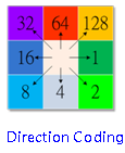
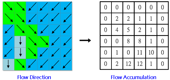
Description of Parameters
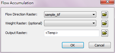
Item
|
Description
|
Data Type
|
Input Direction Raster
|
The direction raster to be performed Flow Accumulation .
|
Raster data
|
Input Weight Raster
|
Limit the output flow by giving weight, the default is 1.
|
Raster data
|
Output Raster
|
The filename and storage path of output raster.
|
Raster data
|
++++++++++++++++++++++++++++++++++++++++++++++++++++++++++++++++++++++++
e- WET ON the system commands the computer's operating system from time to time for ADA
( Address -- Data -- Accumulation ) Station Plan