e- control DIREW on electronic control system circuit , microprocessor , microcontroller so do a series of digital control systems AMNIMARJESLOW GOVERNMENT 91220017 XI XAM PIN PING HUNG CHOP 02096010014 LJBUSAF ___ Thankyume on Lord Jesus Blessing predicate mastery of the system ___ PIT Open Saucer and JESS open Windows ___ Gen. Mac Tech Zone e- Control DIREW 91375

    




                                                     MODERN CONTROL SYSTEM 


A digital computer may serve as a compensator or controller in a feedback control system. Since the computer receives data only at specific intervals, it is necessary to develop a method for describing and analyzing the performance of computer control systems.

The computer system uses data sampled at prespecified intervals, resulting in a time series of signals. These time series, called sampled data, can be transformed to the s-domain and, ultimately, to the z-domain by the relation z = e^ST. The complex frequency domain in terms of zhas properties similar to those of the Laplace s-domain.

We may use the z-transform of a transfer function to analyze the stability and transient response of a system. Thus we may readily determine the response of a closed-loop feedback system with a digital computer serving as the compensator (or controller) block. We can also utilize the root locus method to determine the location of the roots of the characteristic equation. These computer control systems are widely used in industry. They also play an important role in the control of industrial processes, which utilize a combination of a computer and an actuator working together to perform a series of tasks. This chapter concludes with the design of a digital controller for the Sequential Design Example: Disk Drive Read System. 

  

                                             Electronic Systems

It does this with the aid of input devices such as sensors, that respond in some way to this information and then uses electrical energy in the form of an output action to control a physical process or perform some type of mathematical operation on the signal.

But electronic control systems can also be regarded as a process that transforms one signal into another so as to give the desired system response. Then we can say that a simple electronic system consists of an input, a process, and an output with the input variable to the system and the output variable from the system both being signals.

There are many ways to represent a system, for example: mathematically, descriptively, pictorially or schematically. Electronic systems are generally represented schematically as a series of interconnected blocks and signals with each block having its own set of inputs and outputs.

As a result, even the most complex of electronic control systems can be represented by a combination of simple blocks, with each block containing or representing an individual component or complete sub-system. The representing of an electronic system or process control system as a number of interconnected blocks or boxes is known commonly as “block-diagram representation”.

Block Diagram Representation of a Simple Electronic System

Electronic Systems have both Inputs and Outputs with the output or outputs being produced by processing the inputs. Also, the input signal(s) may cause the process to change or may itself cause the operation of the system to change. Therefore the input(s) to a system is the “cause” of the change, while the resulting action that occurs on the systems output due to this cause being present is called the “effect”, with the effect being a consequence of the cause.

In other words, an electronic system can be classed as “causal” in nature as there is a direct relationship between its input and its output. Electronic systems analysis and process control theory are generally based upon this Cause and Effect analysis.

So for example in an audio system, a microphone (input device) causes sound waves to be converted into electrical signals for the amplifier to amplify (a process), and a loudspeaker (output device) produces sound waves as an effect of being driven by the amplifiers electrical signals.

But an electronic system need not be a simple or single operation. It can also be an interconnection of several sub-systems all working together within the same overall system.

Our audio system could for example, involve the connection of a CD player, or a DVD player, an MP3 player, or a radio receiver all being multiple inputs to the same amplifier which in turn drives one or more sets of stereo or home theatre type surround loudspeakers.

But an electronic system can not just be a collection of inputs and outputs, it must “do something”, even if it is just to monitor a switch or to turn “ON” a light. We know that sensors are input devices that detect or turn real world measurements into electronic signals which can then be processed. These electrical signals can be in the form of either voltages or currents within a circuit. The opposite or output device is called an actuator, that converts the processed signal into some operation or action, usually in the form of mechanical movement.

Types of Electronic System

Electronic systems operate on either continuous-time (CT) signals or discrete-time (DT) signals. A continuous-time system is one in which the input signals are defined along a continuum of time, such as an analogue signal which “continues” over time producing a continuous-time signal.

But a continuous-time signal can also vary in magnitude or be periodic in nature with a time period T. As a result, continuous-time electronic systems tend to be purely analogue systems producing a linear operation with both their input and output signals referenced over a set period of time.

For example, the temperature of a room can be classed as a continuous time signal which can be measured between two values or set points, for example from cold to hot or from Monday to Friday. We can represent a continuous-time signal by using the independent variable for time t, and where x(t) represents the input signal and y(t) represents the output signal over a period of time t.

Generally, most of the signals present in the physical world which we can use tend to be continuous-time signals. For example, voltage, current, temperature, pressure, velocity, etc.

On the other hand, a discrete-time system is one in which the input signals are not continuous but a sequence or a series of signal values defined in “discrete” points of time. This results in a discrete-time output generally represented as a sequence of values or numbers.

Generally a discrete signal is specified only at discrete intervals, values or equally spaced points in time. So for example, the temperature of a room measured at 1pm, at 2pm, at 3pm and again at 4pm without regards for the actual room temperature in between these points at say, 1:30pm or at 2:45pm.

However, a continuous-time signal, x(t) can be represented as a discrete set of signals only at discrete intervals or “moments in time”. Discrete signals are not measured versus time, but instead are plotted at discrete time intervals, where n is the sampling interval. As a result discrete-time signals are usually denoted as x(n) representing the input and y(n) representing the output.

Then we can represent the input and output signals of a system as x and y respectively with the signal, or signals themselves being represented by the variable, t, which usually represents time for a continuous system and the variable n, which represents an integervalue for a discrete system as shown.

Continuous-time and Discrete-time System

Interconnection of Systems

One of the practical aspects of electronic systems and block-diagram representation is that they can be combined together in either a series or parallel combinations to form much bigger systems. Many larger real systems are built using the interconnection of several sub-systems and by using block diagrams to represent each subsystem, we can build a graphical representation of the whole system being analysed.

When subsystems are combined to form a series circuit, the overall output at y(t) will be equivalent to the multiplication of the input signal x(t) as shown as the subsystems are cascaded together.

Series Connected System

For a series connected continuous-time system, the output signal y(t) of the first subsystem, “A” becomes the input signal of the second subsystem, “B” whose output becomes the input of the third subsystem, “C” and so on through the series chain giving A x B x C, etc.

Then the original input signal is cascaded through a series connected system, so for two series connected subsystems, the equivalent single output will be equal to the multiplication of the systems, ie, y(t) = G1(s) x G2(s). Where G represents the transfer function of the subsystem.

Note that the term “Transfer Function” of a system refers to and is defined as being the mathematical relationship between the systems input and its output, or output/input and hence describes the behaviour of the system.

Also, for a series connected system, the order in which a series operation is performed does not matter with regards to the input and output signals as: G1(s) x G2(s) is the same as G2(s) x G1(s). An example of a simple series connected circuit could be a single microphone feeding an amplifier followed by a speaker.

Parallel Connected Electronic System

For a parallel connected continuous-time system, each subsystem receives the same input signal, and their individual outputs are summed together to produce an overall output, y(t). Then for two parallel connected subsystems, the equivalent single output will be the sum of the two individual inputs, ie, y(t) = G1(s) + G2(s).

An example of a simple parallel connected circuit could be several microphones feeding into a mixing desk which in turn feeds an amplifier and speaker system.

Electronic Feedback Systems

Another important interconnection of systems which is used extensively in control systems, is the “feedback configuration”. In feedback systems, a fraction of the output signal is “fed back” and either added to or subtracted from the original input signal. The result is that the output of the system is continually altering or updating its input with the purpose of modifying the response of a system to improve stability. A feedback system is also commonly referred to as a “Closed-loop System” as shown.

Closed-Loop Feedback System

Feedback systems are used a lot in most practical electronic system designs to help stabilise the system and to increase its control. If the feedback loop reduces the value of the original signal, the feedback loop is known as “negative feedback”. If the feedback loop adds to the value of the original signal, the feedback loop is known as “positive feedback”.

An example of a simple feedback system could be a thermostatically controlled heating system in the home. If the home is too hot, the feedback loop will switch “OFF” the heating system to make it cooler. If the home is too cold, the feedback loop will switch “ON” the heating system to make it warmer. In this instance, the system comprises of the heating system, the air temperature and the thermostatically controlled feedback loop.

Transfer Function of Systems

Any subsystem can be represented as a simple block with an input and output as shown. Generally, the input is designated as: θi and the output as: θo. The ratio of output over input represents the gain, ( G ) of the subsystem and is therefore defined as: G = θo/θi

In this case, G represents the Transfer Function of the system or subsystem. When discussing electronic systems in terms of their transfer function, the complex operator, s is used, then the equation for the gain is rewritten as: G(s) = θo(s)/θi(s)

Electronic System Summary

We have seen that a simple Electronic System consists of an input, a process, an output and possibly feedback. Electronic systems can be represented using interconnected block diagrams where the lines between each block or subsystem represents both the flow and direction of a signal through the system.

Block diagrams need not represent a simple single system but can represent very complex systems made from many interconnected subsystems. These subsystems can be connected together in series, parallel or combinations of both depending upon the flow of the signals.

We have also seen that electronic signals and systems can be of continuous-time or discrete-time in nature and may be analogue, digital or both. Feedback loops can be used be used to increase or reduce the performance of a particular system by providing better stability and control. Control is the process of making a system variable adhere to a particular value, called the reference value.

In the next tutorial about Electronic Systems, we will look at a types of electronic control system called an Open-loop System which generates an output signal, y(t) based on its present input values and as such does not monitor its output or make adjustments based on the condition of its output.

                                                      XO___XO   Microcontrollers

A microcontroller is a single chip microcomputer made through VLSI fabrication. A microcontroller also called an embedded controller because the microcontroller and its support circuits are often built into, or embedded in, the devices they control. A microcontroller is available in different word lengths like microprocessors (4bit,8bit,16bit,32bit,64bit and 128-bit microcontrollers are available today).

Microcontroller Chip

1) A microcontroller basically contains one or more following components:

• Central processing unit(CPU)
• Random Access Memory)(RAM)
• Read Only Memory(ROM)
• Input/output ports
• Timers and Counters
• Interrupt Controls
• Analog to digital converters
• Digital  analog converters
• Serial interfacing ports
• Oscillatory circuits

2) A microcontroller internally consists of all features required for a computing system and functions as a computer without adding any external digital parts in it.

3) Most of the pins in the microcontroller chip can be made programmable by the user.

4) A microcontroller has many bit handling instructions that can be easily understood by the programmer.

5) A microcontroller is capable of handling Boolean functions.

6) Higher speed and performance.

7) On-chip ROM structure in a microcontroller provides better firmware security.

8 ) Easy to design with low cost and small size.

Microcontroller structure

The basic structure and block diagram of a microcontroller is shown in the fig (1.1).

• CPU

CPU is the brain of a microcontroller. CPU is responsible for fetching the instruction, decodes it, then finally executed. CPU connects every part of a microcontroller into a single system. The primary function of CPU is fetching and decoding instructions. The instruction fetched from program memory must be decoded by the CPU.

• Memory

The function of memory in a microcontroller is the same as a microprocessor. It is used to store data and program. A microcontroller usually has a certain amount of RAM and ROM (EEPROM, EPROM, etc) or flash memories for storing program source codes.

• Parallel input/output ports

Parallel input/output ports are mainly used to drive/interface various devices such as LCD’S, LED’S, printers, memories, etc to a microcontroller.

• Serial ports

Serial ports provide various serial interfaces between a microcontroller and other peripherals like parallel ports.

• Timers/counters

This is the one of the useful function of a microcontroller. A microcontroller may have more than one timer and counters. The timers and counters provide all timing and counting functions inside the microcontroller. The major operations of this section are performed clock functions, modulations, pulse generations, frequency measuring, making oscillations, etc. This also can be used for counting external pulses.

• Analog to Digital Converter (ADC)

ADC converters are used for converting the analog signal to digital form. The input signal in this converter should be in analog form (e.g. sensor output) and the output from this unit is in digital form. The digital output can be used for various digital applications (e.g. measurement devices).

• Digital to Analog Converter (DAC)

DAC perform reversal operation of ADC conversion.DAC converts the digital signal into analog format. It usually used for controlling analog devices like DC motors, various drives, etc.

• Interrupt control

The interrupt control used for providing interrupt (delay) for a working program. The interrupt may be external (activated by using interrupt pin) or internal (by using interrupt instruction during programming).

• Special functioning block

Some microcontrollers used only for some special applications (e.g. space systems and robotics) these controllers containing additional ports to perform such special operations. This considered as special functioning block.

Comparison between Microprocessor and Microcontroller

The main comparison between microprocessor and microcontroller shown in fig (1.2)

Microcontrollers
1	It is only a general purpose computer CPU	It is a microcomputer itself
2	Memory, I/O ports, timers, interrupts are not available inside the chip	All are integrated inside the microcontroller chip
3	This must have many additional digital components to perform its operation	Can function as a microcomputer without any additional components.
4	Systems become bulkier and expensive.	Make the system simple, economic and compact
5	Not capable for handling Boolean functions	Handling Boolean functions
6	Higher accessing time required	Low accessing time
7	Very few pins are programmable	Most of the pins are programmable
8	Very few number of bit handling instructions	Many bit handling instructions
9	Widely Used in modern PC  and laptops	widely in small control systems
E.g.	INTEL 8086,INTEL Pentium series	INTEL8051,89960,PIC16F877

Advantages of Microcontrollers

The main advantages of microcontrollers are given.

a)      Microcontrollers act as a microcomputer without any digital parts.

b)     As the higher integration inside microcontroller reduces cost and size of the system.

c)      Usage of a microcontroller is simple, easy to troubleshoot and system maintaining.

d)     Most of the pins are programmable by the user for performing different functions.

e)      Easily interface additional RAM, ROM,I/O ports.

f)       Low time required for performing operations.

Disadvantages of Microcontrollers

a)      Microcontrollers have got more complex architecture than that of microprocessors.

b)     Only perform a limited number of executions simultaneously.

c)      Mostly used in micro-equipments.

d)     Cannot interface high power devices directly.

Applications

You can find microcontrollers in all kinds of electronic devices these days. Any device that measures, stores, controls, calculates, or displays information must have a microcontroller chip inside. The largest single use for microcontrollers is in the automobile industry (microcontrollers widely used for controlling engines and power controls in automobiles). You can also find microcontrollers inside keyboards, mouse, modems, printers, and other peripherals. In test equipment, microcontrollers make it easy to add features such as the ability to store measurements, to create and store user routines, and to display messages and waveforms. Consumer products that use microcontrollers include digital camcorders, optical players, LCD/LED display units, etc. And these are just a few examples.

Some basic applications of a microcontroller are given below.

a)      Used in biomedical instruments.

b)     Widely used in communication systems.

c)      Used as a peripheral controller in PC.

d)     Used in robotics.

e)      Used in automobile fields.

                   

  CONTROL WITH TIMER ( Count ROLLING WITH TOWARD INTO MEMORY ROUTE )

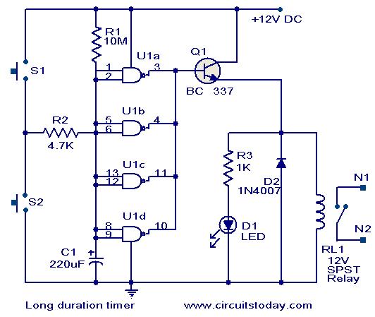
This timer circuit can be used to switch OFF a particular device after around 35 minutes. The circuit can be used to switch OFF devices like radio, TV, fan, pump etc after a preset time of 35 minutes. Such a circuit can surely save a lot of power.

The circuit is based on quad 2 input CMOS IC 4011 (U1).The resistor R1 and capacitor C1 produces the required long time delay. When pushbutton switch S2 is pressed, capacitor C1 discharges and input of the four NAND gates are pulled to zero. The four shorted outputs of U1 go high and activate the transistor Q1 to drive the relay. The appliance connected via the relay is switched ON. When S2 is released the C1 starts charging and when the voltage at its positive pin becomes equal to ½ the supply voltage the outputs of U1 becomes zero and the transistor is switched OFF. This makes the relay deactivated and the appliance connected via the relay is turned OFF. The timer can be made to stop when required by pressing switch S1.

Circuit diagram with Parts list.

Notes.

• Assemble the circuit on a good quality PCB or common board.
  
• The circuit can be powered from a 9V PP3 battery or 12V DC power supply.
  
• The time delay can be varied by varying the values of C1&R1.
  
• The push button switch S2 is for starting the timer and S1 for stopping the time.
  
• The appliance can be connected via contacts N1 & N2 of the relay RL1.
• The IC U1 is 2 input quad NAND gate 4011.

  

          Make a Digital Stop Watch

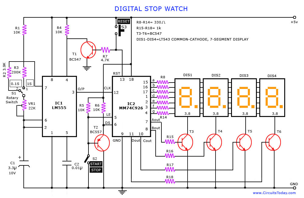
A digital stop watch built around timer IC LM555 and 4-digit counter IC MM74C926  with multiplexed 7-segment LED display. MM74C926 consists of a 4-digit counter, an internal output latch, npn output sourcing drivers for common cathode, 7-segment display and an internal multiplexing circuitry with four multiplexing outputs. The counter advances on negative edge of the clock. The clock is generated by timer IC LM555. The circuit works off a 5V power supply. It can be easily assembled on a general-purpose PCB. Enclose the circuit in a metal box with provisions for four 7-segment displays, rotary switch S1, start/stop switch S2 and reset switch S3

Testing

First, reset the circuit by pressing S3 so that the display shows ‘0000.’ Now open switch S2 for the stop watch to start counting the time. If you want to stop the clock, close S2. Rotary switch S1 is used to select the different time periods at the output of the astable multivibrator (IC1).

Digital Timer Circuit Diagram .

          

               Voltage Multipliers

Voltage multiplier is a modified capacitor filter circuit that delivers a dc voltage twice or rnore times of the peak value (amplitude) of the input ac voltage. Such power supplies are used for high-voltage and low-current devices

 such as cathode-ray tubes (the picture tubes in TV receivers, oscilloscopes and computer display). Here we will consider half-wave voltage doubler, full-wave voltage doubler and voltage tripler and quadrupler.

Half-Wave Voltage Doubler

The circuit of a half-wave voltage doubler is given in figure shown below. During the positive half cycle of the ac input, voltage, diode D₁ being forward biased conducts (diode D₂ does not con­duct because it is reverse-biased) and charges capacitor C₁ upto peak values of secondary voltage V_smax with the polar­ity, as marked in figure shown below.

Half-wave voltage doubler

During the negative half-cycle of the input voltage diode D₂ gets forward biased and conducts charging capacitor C₂. For the negative half cycle, the lower end of the transformer secondary is positive while upper end is negative. The polarity of the capacitor C­₂ has also been marked in the figure. Now starting from the bottom of the transformer secondary and moving clockwise and applying Kirchhoffs voltage law to the outer loop we have

-V_smax – V_c1 + V_c2 = 0

Or

V_c2 = V_smax + V_c1= Vsmax + Vsmax = 2V_smax = Twice the peak value of the transformer secondary voltage. (Since V_c1 = V_smax)

During the next positive half-.cycle diode D₂ is reverse-biased and so acts as an open and capacitor C₂ discharges through the load If there is no load across the capacitor, C₂ both capacitors stay charged – C₁ to V_smax and C₂ to 2V_smax. If, as expected there is a load connected to the output terminals of the voltage doubler, the capacitor C₂ discharges a little bit and consequently the voltage across capacitor C₂ drops slightly. The capacitor C₂ gets recharged again in the next half-cycle. The ripple frequency in this case will be the signal frequency (that is, 50 Hz for supply mains.)

Full-Wave Voltage Doubler

The circuit diagram for a full-wave voltage doubler is given in the figure shown below. During the positive cycle of the ac input voltage, diode D₁ gets forward biased and so conducts charging the capacitor C₁ to a peak voltage V_smax with polarity indicated in the figure, while diode D₂ is reverse-biased and does not conduct.During the negative half-cycle, diode D₂ being forward biased conducts and charges the capacitor C₂ with polarity shown in the figure while diode D₁does not conduct. With no load connected to the output terminals, the output voltage will be equal to sum of voltages across capacitors C₁ and C₂ that is, V_C1 + V_C2 or (V_s max + V_s max) or 2 V_s max. When the load is connected to the output terminals, the output voltage V_L will be somewhat less than 2 V_s max. The input voltage and output voltage waveforms are also shown in the figure below.

Full-wave voltage doubler

Take a look : Comparison Between Half-wave and Full-wave Voltage Doublers

Voltage Tripler and Quadruples

The half-wave voltage doubler, shown in the earlier figure can be extended to provide any multiple of the peak input voltage (that is, 3 V_s max, 4 V_s max or 5 V_s max), as illustrated in the figure shown below. It is obvious from the pattern of the circuit connections how additional diodes and capacitors are to be connected to provide output voltage, 5,6,7 or 8 times the peak input voltage from a supply transformer of rating only V_s max, and each diode in the circuit of PIV rating 2 V_s max. If load is small and the capacitors have little leakage, extremely high dc voltages can be obtained from such a circuit using many sections to step-up the dc voltage.

In operation capacitor C₁ is charged through diode D_l to a peak value of transformer secondary voltage, V_s max during first positive half-cycle of the ac input voltage. During the negative half cycle capacitor C₂ is charged to twice the peak voltage 2 V_s developed by the sum of voltages across capacitor C₁ and the transformer secondary. During the second positive half-cycle, diode D₃ conducts and the voltage across capacitor C₂ charges the capacitor C₃ to the same 2 V_g maxpeak voltage. During the negative half-cycle diodes D₂ and D₄ conduct allowing capacitor C₃ to charge capacitor C₄ to peak voltage 2 V_{S max}. From the fogure shown below it is obvious that the voltage across capacitor C₂ is 2 V_{s max}, across capacitors C₁ and C₃ it is 3 V_s max and across capacitors C₂ and C₄ it is 4 V_s max.

If additional diodes (each diode of PIV rating 2 V_s max) and capacitors (each capacitor of voltage rating 2 V_s max) are used, each capacitor will be charged to 2 V_{s max}. Measuring from the top of the transformer secondary winding (figure below) will give odd multiples of V_g max at the output, while measuring from the bottom of transformer secondary winding will give even multiples of the peak voltage, V_s max.

Voltage Tripler and Quadruplar

Some electronic devices, such as cathode ray tubes (in picture tubes in TV receivers, oscilloscopes and computer display) need dc power supply at high voltage with low current. This requirement can be met with either by employing a step-up transformer with a rectifier circuit or by employing voltage multiplier. Since transformers are very bulky and costly, voltage multipliers are preferred. By using voltage multipliers, the voltage level is usually raised well into the hundreds or thousands of volts. 

   

            Static 0 to 9 display

The circuit shown here is of a simple 0 to 9 display that can be employed in a lot of applications. The circuit is based on asynchronous decade counter 7490(IC2), a 7 segment display (D1), and a seven segment decoder/driver IC 7446 (IC1).
The seven segment display consists of 7 LEDs labelled ‘a’ through ‘g’. By forward biasing different LEDs, we can display the digits 0 through 9. Seven segment displays are of two types, common cathode and common anode. In common anode type anodes of all the seven LEDs are tied together, while in common cathode type all cathodes are tied together. The seven segment display used here is a common anode type .Resistor R1 to R7 are current limiting resistors. IC 7446 is a decoder/driver IC used to drive the seven segment display.
Working of this circuit is very simple. For every clock pulse the BCD output of the IC2 (7490) will advance by one bit. The IC1 (7446) will decode this BCD output to corresponding the seven segment form and will drive the display to indicate the corresponding digit.

Circuit diagram.

Notes.

• The circuit can be assembled on a perf board.
• Use 5V DC for powering the circuit.
• The clock can be given to the pin 14 of IC2.
• D1 must be a seven segment common anode display.
• All ICs must be mounted on holders.

            Triggering of Flip Flops     

 the importance of triggering a flip flop. The output of a flip flop can be changed by bring a small change in the input signal. This small change can be brought with the help of a clock pulse or commonly known as a trigger pulse.

When such a trigger pulse is applied to the input, the output changes and thus the flip flop is said to be triggered. Flip flops are applicable in designing counters or registers which stores data in the form of multi-bit numbers.But such registers need a group of flip flops connected to each other as sequential circuits. And these sequential circuits require trigger pulses.

The number of trigger pulses that is applied to the input of the circuit determines the number in a counter. A single pulse makes the bit move one position, when it is applied onto a register that stores multi-bit data.

In the case of SR Flip Flops, the change in signal level decides the type of trigger that is to be given to the input. But the original level must be regained before giving a second pulse to the circuit.

If a clock pulse is given to the input of the flip flop at the same time when the output of the flip flop is changing, it may cause instability to the circuit. The reason for this instability is the feedback that is given from the output combinational circuit to the memory elements. This problem can be solved to a certain level  by making the flip flop more sensitive to the pulse transition rather than the pulse duration.

There are mainly four types of pulse-triggering methods. They differ in the manner in which the electronic circuits respond to the pulse. They are

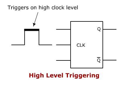
1. High Level Triggering

When a flip flop is required to respond at its HIGH state,  a HIGH level triggering method is used. It is mainly identified from the straight lead from the clock input. Take a look at the symbolic representation shown below.

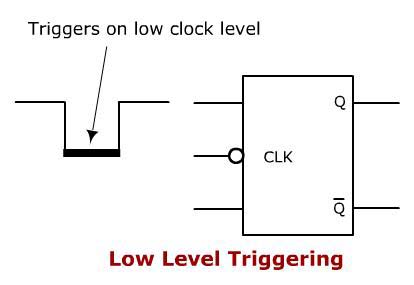
2. Low Level Triggering

When a flip flop is required to respond at its LOW state,  a LOW level triggering method is used.. It is mainly identified from the clock input lead along with a low state indicator bubble. Take a look at the symbolic representation shown below.

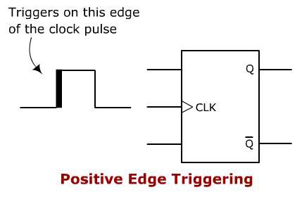
3. Positive Edge Triggering

When a flip flop is required to respond at a LOW to HIGH transition state,  POSITIVE edge triggering method is used. It is mainly identified from the clock input lead along with a triangle. Take a look at the symbolic representation shown below.

4. Negative Edge Triggering

When a flip flop is required to respond during the HIGH to LOW transition state,  a NEGATIVE edge triggering method is used.. It is mainly identified from the clock input lead along with a low-state indicator and a triangle. Take a look at the symbolic representation shown below.

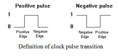
Clock Pulse Transition

The movement of a trigger pulse is always from a 0 to 1 and then 1 to 0 of a signal. Thus it takes two transitions in a single signal. When it moves from 0 to 1 it is called a positive transition and when it moves from 1 to 0 it is called a negative transition. To understand more take a look at the images below.

The clocked flip-flops already introduced are triggered during the 0 to 1 transition of the pulse, and the state transition starts as soon as the pulse reaches the HIGH level. If the other inputs change while the clock is still 1, a new output state may occur. If the flip-flop is made to then the multiple-transition problem can be eliminated.

The multi-transition problem can be stopped is the flip flop is made to respond to the positive or negative edge transition only, other than responding to the entire pulse duration.

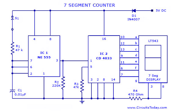
      Seven Segment Counter Display Circuit    

the circuit diagram of a seven segment counter based on the counter IC CD 4033.This circuit can be used in conjunction with various circuits where a counter to display the progress  adds some more attraction.

IC NE 555 is wired as an astable multivibrator for triggering the CD 4033.For each pulse the out put of CD 4033 advances by one count.The output of CD 4033 is displayed by the seven segment LED display LT543.Switch S1 is used to initiate the counting.Diode D1 prevents the risk of accidental polarity reversal.

Seven Segment Circuit Diagram with Parts List.

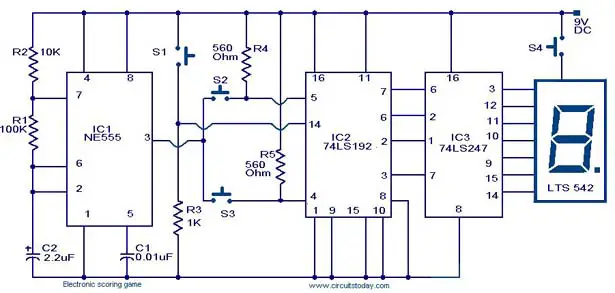
            Scoring game circuit              

A simple scoring game circuit that can be used for all occasions when a dice is needed.The circuit is based on a NE555 timer,a 74LS192 counter,a74LS247 decoder and a & segment LED display.The timer IC1 will produce the clock for the counter IC(IC2) whose frequency is determined by R1 and C2.When S2 is pressed the IC2 will count in up mode and when S3 is pressed the IC2 will count in down mode.The IC 3 will decode the count to display it on the seven segment LED display .Thats about the working of the circuit.The circuit is designed strictly sticking on to the basics of counters and is a good one for beginners.There is nothing big deal.

Circuit diagram with Parts list.

Notes.

• To play the game switch the power ON and press S1 to reset the counter.
• Now press S2 or S3 and release .The IC2 will hold the last count .Now press S4 to see the score on display.That’s your score.Now the second person can try.
• Each time one tries, he should press the S1 to reset the count and then press S2 or S3 and then S4 to see the score.
• Circuit can be powered from a 9V radio cell or a 9V regulated DC power supply .

  Different Types Of Digital Cameras  

Digital cameras are mainly classified according to their use, automatic and manual focus, and also price. Here are the classifications.

1. Compact digital cameras

Compact cameras are the most widely used and the simplest cameras to be ever seen. They are used for ordinary purposes and are thus called “point and shoot cameras”. They are very small in size and are hence portable. Since they are cheaper than the other cameras, they also contain fewer features, thus lessening the picture quality. These cameras are further classified according to their size. The smaller cameras are generally called as ultra-compact cameras. The others are called compact cameras.

Here are some features of this camera

• Compact and simple.
• Images can be stored in computer as JPEG files.
• Live preview can be seen before taking photos.
• Low power flashes are available for taking photos in the dark.
• Contains auto-focus system with closer focusing ability.
• Zoom capability.

Although these features are available, their magnitude may be less compared to other cameras. The flashes may be available only for nearby objects. The preview of the picture to be taken will have less motion capability.  The image sensors used in these cameras have a very small diognal space of about 6mm with a crop factor of 6.

Compact Digital Cameras

2. Bridge cameras

Bridge cameras are most often mistaken for single-lens reflex cameras (SLR). Though they have the same characteristics their features are different. Some of its features are

• Fixed lens
• Small image sensors
• Live preview of the image to be taken
• Auto-focus using contrast-detect method and also manual focus.
• Image stabilization method to reduce sensitivity.
• Image can be stored as a raw data as well as compressed JPEG format.

Though they resemble SLR in many ways, they operate much slower than the latter. They are very big in size and so the fixed lenses are given very high zooming capability and also fast apertures. The autofocus or manual focus is set according to our necessity. The image preview is done using either a LCD or an Electronic View Finder (EVF).

Bridge Cameras

3. Digital single lens reflex cameras (DSLR)

This is one of the most high end cameras obtainable for a decent price. They use the single-lens reflex method just like an ordinary camera with a digital image sensor. The SLR method consists of a mirror which reflects the light passing through the lens with the help of a separate optical viewfinder.

Some features of this camera are

• Special type of sensors is setup in the mirror box for obtaining autofocus.
• Has live preview mode.
• Very high end sensors with crop factors from 2 to 1 with diagonal space from 18mm to 36mm.
• High picture quality even at low light.
• The depth of field is very less at a particular aperture.
• The photographer can choose the lens needed for the situation and can also be easily interchangeable.
• A focal plane shutter is used in front of the imager.
• 

  Digital single lens reflex cameras (DSLR)

4. Electronic viewfinder (EVF)

This is just a combination of very large sensors and also interchangeable lenses. The preview is made using an EVF. There is no complication in mechanism like a DSLR.

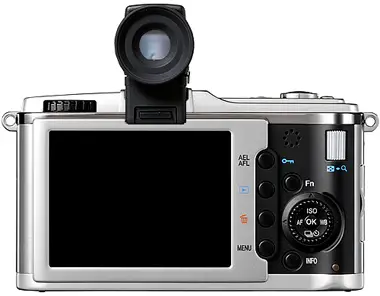
Electronic View Finder

5. Digital rangefinders

This is a special film camera equipped with a rangefinder. With this type of a camera distant photography is possible. Though other cameras can be used to take distant photos, they do not use the rangefinder technique.

Digital rangefinders

6. Line-scan cameras

This type of cameras is used for capturing high image resolutions at a very high speed. To make this mechanism possible, a single pixel of image sensors are used instead of a matrix system. A stream of pictures of constantly moving materials can be taken with this camera. The data produced by a line-scan camera is 1-dimensional. It has to be processed in a computer to make it 2-D. This 2-D data is further processed to obtain our needs.

                     State space analysis.               

State space analysis is an excellent method for the design and analysis of control systems. The conventional and old method for the design and analysis of control systems is the transfer function method. The transfer function method for design and analysis had many drawbacks.

Drawbacks of transfer function analysis.

• Transfer function is defined under zero initial conditions.
• Transfer function approach can be applied only to linear time invariant systems.
• It does not give any idea about the internal state of the system.
• It cannot be applied to multiple input multiple output systems.
• It is comparatively difficult to perform transfer function analysis on computers.

Any way state variable analysis can be performed on any type systems and it is very easy to perform state variable analysis on computers. The most interesting feature of state space analysis is that the state variable we choose for describing the system need not be physical quantities related to the system. Variables that are not related to the physical quantities associated with the system can be also selected as the state variables. Even variables that are immeasurable or unobservable can be selected as state variables.

Advantages of state variable analysis.

• It can be applied to non linear system.
• It can be applied to tile invariant systems.
• It can be applied to multiple input multiple output systems.
• Its gives idea about the internal state of the system.

State of a dynamic system.

The state of a system is the minimum set of variables (state variables) whose knowledge at time t=0, along with the knowledge of the inputs at time t≥ t0 completely describes the behaviour of a dynamic system for a time t >t0 . State variable is a set of variables which fully describes a dynamic system at a given instant of time.

Consider a system having a inputs, b outputs and c state variables. Then,

Output variables = Y1(t), Y2(t), Y3(t)…………………………..Yb(t)

Input variables  = U1(t), U2(t), U3(t)……………………………Ua(t)

State variables =   X1(t), X2(t), X3(t) …………………………….Xc(t)

Then the system can be represented as shown below.

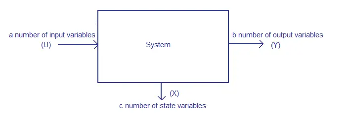
State space representation of a system

         Working of Digital Cameras        

the working of a camera. Almost all the basics of this post have been explained there. Now let us know more about a digital camera, its working, and also advantages.

The digital camera can be considered as an alteration of the conventional analog camera. Most of the associated components are also the same, except that instead of light falling on a photosensitive film like an analog camera, image sensors are used in digital cameras. Though analog cameras are mostly dependent on mechanical and chemical processes, digital cameras are dependent on digital processes. This is a major shift from its predecessor as the concept of saving and sharing audio as well as video contents have been simplified to earth. 

Digital Camera Basics

As told earlier, the basic components are all the same for both analog and digital cameras. But, the only difference is that the images received in an analog camera will be printed on a photographic paper. If you need to send these photos by mail, you will have to digitally convert them. So, the photo has to be digitally scanned.

This difficulty is not seen in digital photos. The photos from a digital camera are already in the digital format which the computer can easily recognize (0 and 1). The 0’s and 1’s in a digital camera are kept as strings of tiny dots called pixels.

The image sensors used in an digital can be either a Charge Coupled Device (CCD) or a Complimentary Metal Oxide Semi-conductor (CMOS). Both these image sensors have been deeply explained earlier.

The image sensor is basically a micro-chip with a width of about 10mm. The chip consists arrays of sensors, which can convert the light into electrical charges. Though both CMOS and CCD are very common, CMOS chips are known to be more cheaper. But for higher pixel range and costly cameras mostly CCD technology is used.

A digital camera has lens/lenses which are used to focus the light that is to be projected and created. This light is made to focus on an image sensor which converts the light signals into electric signals. The light hits the image sensor as soon as the photographer hits the shutter button. As soon as the shutter opens the pixels are illuminated by the light in different intensities. Thus an electric signal is generated. This electric signal is then further broke down to digital data and stored in a computer.

Pixel Resolution of a Digital Camera

The clarity of the photos taken from a digital camera depends on the resolution of the camera. This resolution is always measured in the pixels. If the numbers of pixels are more, the resolution increases, thereby increasing the picture quality. There are many type of resolutions available for cameras. They differ mainly in the price.

• 256×256 – This is the basic resolution a camera has. The images taken in such a resolution will look blurred and grainy. They are the cheapest and also unacceptable.
• 640×480 – This is a little more high resolution camera than 256×256 type. Though a clearer image than the former can be obtained, they are frequently considered to be low end. These type of cameras are suitable for posting pics and images in websites.
• 1216×912 – This resolution is normally used in studios for printing pictures. A total of 1,109,000 pixels are available.
• 1600×1200 – This is the high resolution type. The pictures are in their high end and can be used to make a 4×5 with the same quality as that you would get from a photo lab.
• 2240×1680 – This is commonly referred to as a 4 megapixel cameras. With this resolution you can easily take a photo print up to 16×20 inches.
• 4064×2704 – This is commonly referred to as a 11.1 megapixel camera. 11.1 megapixels takes pictures at this resolution. With this resolution you can easily take a photo print up to 13.5×9 inch prints with no loss of picture quality.
• There are even higher resolution cameras up to 20 million pixels or so.

Color Filtering using Demosaicing Algorithms

The sensors used in digital cameras are actually coloured blind. All it knows is to keep a track of the intensity of light hitting on it. To get the colour image, the photosites use filters so as to obtain the three primary colours. Once these colours are combined the required spectrum is obtained.

For this, a mechanism called interpolation is carried out. A colour filter array is placed over each individual photosite. Thus, the sensor is divided into red, green and blue pixels providing accurate result of the true colour at a particular location. The filter most commonly used for this process is called Bayer filter pattern. In this pattern an alternative row of red and green filters with a row of blue and green filters. The number of green pixels available will be equal to the number of blue and red combined. It is designed in a different proportion as the human eye is not equally sensitive to all three colours. Our eyes will percept a true vision only if the green pixels are more.

The main advantage of this method is that only one sensor is required for the recording of all the colour information. Thus the size of the camera as well as its price can be lessened to a great extent. Thus by using a Bayer Filter a mosaic of all the main colours are obtained in various intensities. These various intensities can be further simplified into equal sized mosaics through a method called demosaicing algorithms. For this the three composite colours from a single pixel are mixed to form a single true colour by finding out the average values of the closest surrounding pixels.

Take a look at the digital camera schematic shown below.

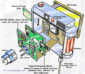
Digital Camera Diagram

Parameters of a Digital Camera

Like a film camera, a digital camera also has certain parameters. These parameters decide the clarity of the image. First of all the amount of light that enters through the lens and hits the sensor has to be controlled. For this, the parameters are

1. Aperture – Aperture refers to the diameter of the opening in the camera. This can be set in automatic as well as the manual mode. Professionals prefer manual mode, as they can bring their own touch to the image.

2. Shutter Speed – Shutter speed refers to the rate and amount of light that passes through the aperture. This can be automatic only. Both the aperture and the shutter speed play important roles in making a good image.

3. Focal Length – The focal length is a factor that is designed by the manufacturer. It is the distance between the lens and the sensor. It also depends on the size of the sensor. If the size of the sensor is small, the focal length will also be reduced by a proportional amount.

4. Lens – There are mainly four types of lenses used for a digital camera. They differ according to the cost of the camera, and also focal length adjustment. They are

• Fixed-focus, fixed-zoom lens – They are very common and are used in inexpensive cameras.
• Optical-zoom lenses with automatic focus – These are lenses with focal length adjustments. They also have the “wide” and “telephoto” options.
• Digital zoom – Full-sized images are produced by taking pixels from the centre of the image sensor. This method also depends on the resolution as well as the sensor used in the camera.
• Replaceable lens systems – Some digital cameras replace their lenses with 35mm camera lenses so as to obtain better images.

Digital Cameras v/s Analog Camera

• The picture quality obtained in a film camera is much better than that in a digital camera.
• The rise of technology has made filming the help of digital techniques easier as well as popular.
• Since the digtal copy can be posted in websites, photos can be sent to anyone in this world.

Though both of them are equally used in cameras, there are some differences in parameters like gain, speed and so on.

Comparison –  Charge Coupled Device and CMOS Active Pixel Sensor

• Both the devices are used to convert light into electric signals and are used for the same applications.  After converting the signals, they have to be read from each cell. This process is different for both the devices.

• The charge from each chip is taken to the end of the array and then read in a CCD. This is then converted into a digital signal with the help of an analog to digital converter (ADC). The process of reading the signal by CMOS Active Pixel Sensor is done by using transistors and amplifiers at each pixel and then the signal is moved using traditional wires.

Difference – Charge Coupled Device and CMOS Active Pixel Sensor

• CCD image sensors create super quality pictures. They also produce lesser noise than CMOS APS.

• In a CMOS all the transistors are kept right next to each pixel. As a result, all the photons that hit the device actually get scattered by hitting the transistors as well. Thus, the sensitivity of CMOS Active Pixel Sensor is lesser than that of a Charge Coupled Device.

• The design of the CCD sensors is in such a way that they require more power for its operation. If both the devices of equal reception are taken, the CCD is considered to consume almost 100 times more power than its equivalent CMOS Active Pixel Sensor.

• All the devices have been using Charge Coupled Device devices far more than CMOS Active Pixel Sensor. As a result a vast study has been done on CCD devices. So, they are more mature and also tend to have higher quality pixels.

Active Pixel Sensor (APS) is an image sensor, made up of an array of pixel sensors. In these pixel sensors, each pixel sensor consists of a photo detector and an amplifier. Out of these APS, the most notable is the CMOS Active Pixel Sensor (CMOS APS). CMOS APS has great applications in cameras and also DSLRs. It is called so as it is manufactured by the CMOS process. This type of image sensor is very similar to that of a Charge Coupled Device (CCD). They are also called active pixel sensor imager and also active pixel image sensor.

The CMOS APS uses a photo detector to detect the light and converts it into electrical signal. This signal is then amplified using several transistors and is then moved using traditional wires.

Introduction of CMOS Active Pixel Sensors

The wide use of CMOS Active Pixel Sensors began during the year 1993. The Jet Propulsion Laboratory developed some prototypes which were later commercialized. After knowing its immense potential in the field high speed, low power motion capture cameras many companies quickly adopted and developed this technology.

During the early 1960’s, before the discovery of active pixel sensors, there were only passive pixel sensors. In this mechanism, the pixels were designed in a 2D structure, with access enable wire shared by pixels in the same row, and output wire shared by column. Each pixel did not have an amplifier and so an amplifier was connected ar the end of each column. High power consumption, greater noise and also slow output were some of its disadvantages. In 1969, the active pixel sensor was first introduced by adding independent amplifiers for each pixel. Thus in 1970, the Charge Coupled Device was invented. Thus they were very useful in the working of cameras. During the early 1990’s the CMOS process was well developed and was considered to be the base for all types of logic devices as well as microprocessors. This further led to the invention of CMOS APS.

Architecture of Active Pixel Sensors

For describing the architecture of a CMOS APS, there are mainly three different parameters. They are

• Pixel

The pixel of a CMOS APS mainly consists of photo detectors like a JFET photogate or pinned photodiode. The whole pixel will be called a 4T (4 transistor) cell. The 4T cell mainly consists of a transfer gate, reset gate, selection gate and also a source follower input transistor connected to the photo detector.

The photo detectors used in this 4T cell were first used for Charge Coupled Devices. But, when it was further connected it to the transfer gate and other components the charge transfer was done at a greater speed and also low noise was generated.

There are 3 transistor (3T) cells used now as well. As they are very simple in fabrication they are more commercially produced.

• Thin Film Transistor APS

APS has applications in the field of X-ray as well. For taking digital X-rays, thin film transistors (TFT) is also used. But, its larger size and low gain makes the number of TFTs limited.

• Array

A 2-D array of pixels is organized into rows and columns. The reset lines are connected to the rows so that when RESET occurs the whole row gets reset. Similar is the case of the select lines. The outputs of each pixel in any given column are tied together. Take a look at the architectural diagram given below.

CMOS active pixel transisitor

Applications

The applications of CMOS APS includes web cameras, motion capture cameras, digital radiography, endoscopy cameras and also X-ray imaging. They are mainly known for their application in filmless cameras.

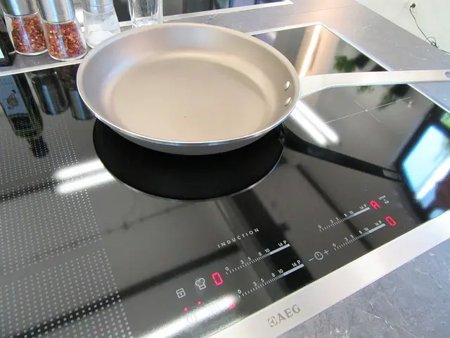
            Working of induction cooktops            

cooktops are very popular in all households. They have lots of advantages over gas and electric cooktops and are more efficient. But have you ever wondered how an induction cooktop works?

The working of an induction cooktop is very simple. It has more to do with electrical engineering than electronics but this caught my eye because an induction cooktop, a product that has a billion dollar market, uses a very base level technology for its working. How amazing is that such simple things can change our lives.

The Science behind induction cooktops

Induction cooktops work using the principle of Magnetic Induction

I am sure you have heard the terms magnetic fields and eddy currents. When current passes through a coil a magnetic field is produced around it. If the current use is AC (Alternating Current) the magnetic field produced keep changing its direction. When an electric conductor is placed in this alternating magnetic field the magnetic lines cut through the surface of the conductor. This generate eddy currents. Eddy currents are basically electricity produced within a conductor due to the presence of an alternating magnetic field and these currents flow in loops through the conductor. Due to the resistance of the material these eddy currents produce heat. This is the basic working principle of induction cooktops

An induction cooktop has two main parts;

1) Induction coil

2) Cookware

Induction coils are made of copper and they produce a highly alternating magnetic field. The cookware does the job of the electric conductor but for this to be done it has to be ferrous. The presence of iron content in the cookware is important because only ferrous materials produce eddy currents when in contact with an alternating magnetic field. The heat for cooking is produced by eddy currents inside the cooking vessel and is passed through the food by conduction.

You can easily check if a cookware is ferrous or not by bringing a magnet near it, if it sticks then the cookware is ferrous. Induction cooktops also have control panels to control temperature, cooking time and other various aspects. 

Unlike other methods of cooking here the heat is produced inside the cooking vessel which reduces any heat loss so the system is very efficient. There are hundreds of these now available in the market.

Controllability and Observability.

Controllability and observability are two very important things related to state space analysis. There are many tests for checking controllability and obervability and these tests are very essential during the design of a control system using state space approach.

Controllability.

Controllability verifies whether is state variable is useful or not. It checks whether a state variable can be manipulated for obtaining the required output. If a state variable is not controllable then there is no meaning in selecting it for any operation. If a particular state variable is found uncontrollable , then it is left untouched and any other state variable which is controllable is selected for operations.

A system is said to be completely state controllable if it is possible to change the system from any initial stage X(t0) to any required stage X(td) using a control vector U(t). Kalman’s test and Gilberts test are the two common methods used for testing controllability.

Gilberts method.

Gilbert’s method for checking controllability is done under two cases.

1)When the eigen values of the system matrix are distinct.

In this case the system matrix can be diagonalized and can be converted to the canonical form by giving a transformation X=MZ. M is the modal matrix derived from the system matrix and Z is the transformed state variable matrix.

Consider a system with state model represented by the equations

X = AX + BU

Y = CX + DU

The model is transformed into the canonical form as follows,

Z = ΛZ + B˜U

Y = C˜Z + DU

Where Λ= MA¯¹M,   B˜ = M¯¹B and C˜ = CM

The system is completely state controllable if the matrix B doesnot have any row with all zeros.

2) Eigen values of the system matrix are repeated.

In this situation it is impossible to diagonalize the system matrix and it can be converted to Jordan canonical form.

Consider a system with state model represented by the equations

X = AX + BU

Y = CX + DU

The model is transformed into the Jordan canonical form as follows,

Z = JZ + Β˜U

Y = C˜Z + DU

Where J = M A¯¹M,   B˜ = M¯¹B and C˜ = CM

The system will be completely state controllable if elements of any row of B that correspond to the last row of each Jordan block are not all zero and the rows corresponding to other state variables must not have all zeros.

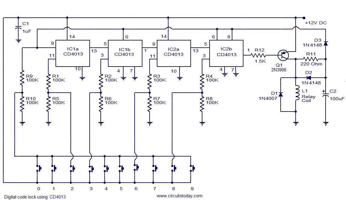
                 Digital code lock                

 a simple but effective code lock circuit that has an automatic reset facility. The circuit is made around the dual flip-flop IC CD4013.Two CD 4013 ICs are used here. Push button switches are used for entering the code number. One side of all the push button switches are connected to +12V DC. The remaining end of push buttons 2,3,6,8 is connected to clock input pins of the filp-flops. The remaining end of other push button switches are shorted and connected to the set pin of the filp-flops.
The relay coil will be activated only if the code is entered in correct sequence and if there is any variation, the lock will be resetted. Here is correct code is 2368.When you press 2 the first flip flop(IC1a) will be triggered and the value at the data in (pin9) will be transferred to the Q output (pin13).Since pin 9 is grounded the value is “0” and so the pin 13 becomes low. For the subsequent pressing of the remaining code digits in the correct sequence the “0” will reach the Q output (pin1) of the last flip flop (IC2b).This makes the transistor ON and the relay is energised.The automatic reset facility is achieved by the resistor R11 and capacitor C2.The positive end of capacitor C2 is connected to the set pin of the filp-flops.When the transistor is switched ON, the capacitor C2 begins to charge and when the voltage across it becomes sufficient the flip-flops are resetted. This makes the lock open for a fixed amount of time and then it locks automatically. The time delay can be adjusted by varying the values of R11 and C2.

Circuit diagram with Parts list.

Notes.

• Assemble the circuit on a good quality PCB.
• The circuit can be powered from 12V DC.
• Mount the ICs on holders.
• The L1 can be a 12V, 200 Ohm SPDT relay.
• Capacitor C1 should be tantalum type.
• The C1 and C2 must be rated at least 25V.

Electronic Combination Lock Circuit

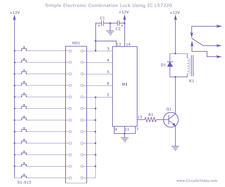
 the circuit diagram of a simple electronic combination lock using IC LS 7220.This circuit can be used to activate a relay for controlling (on & off) any device when a preset combination of 4 digits are pressed.The circuit can be operated from 5V to 12V.

To set the combination connect the appropriate switches to pin 3,4,5 and 6 of the IC through the header.As an example if S1 is connected to pin 3, S2 to pin 4 , S3 to pin 5, S4 to pin 6 of the IC ,the combination will be 1234.This way we can create any 4 digit combinations.Then connect the rest of the switches to pin 2 of IC.This will cause the IC to reset if any invalid key is pressed , and entire key code has to be re entered.

When the correct key combination is pressed the out put ( relay) will be activated for a preset time determined by the capacitor C1.Here it is set to be 6S.Increase C1 to increase on time.

For the key pad, arrange switches in a 3X4 matrix on a PCB.Write the digits on the keys using a marker.Instead of using numbers I wrote some symbols!.The bad guys will be more confused by this.

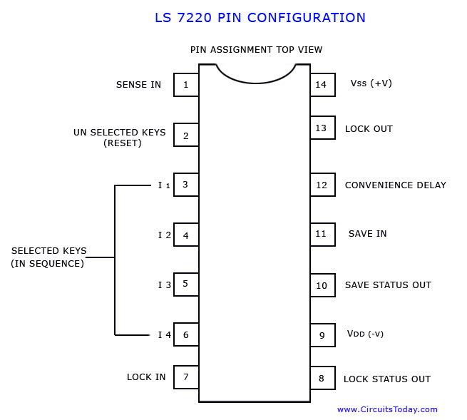
Pin Assignment of LS7220.

Parts List

C1              1   1uF 25V Electrolytic Capacitor
C2              1    220uF 25V Electrolytic Capacitor
R1              1    2.2K 1/4W Resistor
Q1              1    2N3904 NPN Transistor    2N2222
D1              1    1N4148 Rectifier Diode    1N4001-1N4007
K1              1    12V SPDT Relay    Any appropriate relay with 12V coil
U1             1     LS7220 Digital Lock IC
S1-S12    12    SPST Momentary Pushbutton    Keypad (see notes)
HD1          1    12 Position Header

                           Lovotics – A New Robot Race that can Love!!                            

Lovotics

Humans have designed robots for making our tasks easier and simpler. These robots have been used in factories and even at homes as they can work tirelessly everyday and every time and that too without the need of money and food. Till now, no one has ever developed a robot that has the basic human emotions like crying, singing, laughing, dancing, affectionate, angriness, and so on. Of course, we have seen such robots in movies (Bicentennial Man). but in real life…not a chance!!

But, recently, some technicians at the National University of Singapore developed a  robot prototype called Lovotics that can express all these feelings. This robot has the ability to love and to be loved by humans. To develop such a machine, all they did was create a new robot with human behaviour by adding all humanly similar biological and emotional tools.

This may sound complicated, but all the complex hormones that are responsible for a human to get emotions and feelings are given to the robot. These artificial hormones include dopamine, serotonine, oxytocin and endorphin. Apart from these hormones, artificial intelligence process was also conducted to pass on brain signals using MRI scans so that the robots get a better idea on when to react for any kind of emotion.

The robot is taught well to interact with other humans and create emotions like laughter and many more at the right moment, according to the behaviour of the human it is interacting with. During this interaction, touching another analog to affectionate human interaction is very important. .

Just like any other robot, this one will also have the basic structural materials like a a processor with controller and wireless board, a flexible structure, batteries, touch sensors, microphones, an omni-directional base, servo motors, speakers and also LED’s.

                         SPHERES                     

Synchronized Position Hold, Engage, Reorient Experimental Satellites (SPHERES)

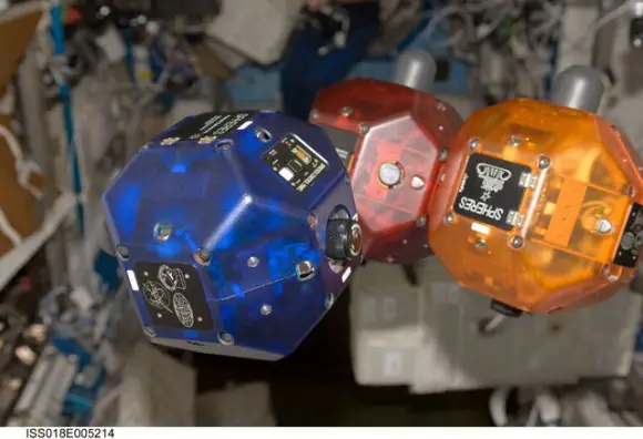
Synchronized Position Hold, Engage, Reorient Experimental Satellites (SPHERES)

SPHERES stands for Synchronized Position Hold, Engage, Reorient Experimental Satellites. This type of NASA Robot mainly consists of 3 miniaturized satellites that can work in extreme climates and environments. These satellites have 8-inch diameters and were originally used in the International Space Station (ISS).

The SPHERE was developed by the Massachusetts Institute of Technology (MIT) Space Systems Laboratory along with Aurora Flight Sciences with high end funding from the Department of Defense and several NASA centres. They wanted to provide the US Air Force and NASA with a long term, renewable, and upgradable platform for formation flight. The main purpose of such a robot is to work in high risk conditions, metrology, and autonomy technologies.

Structure and Design of SPHERES

• The robot has 3 satellites which are micro-sized.
• These satellites are used to control the relative positions and orientations.
• It was made compatible for a 2-D laboratory platform, NASA’s KC-135, and the International Space Station.
• The robot is battery powered and during initial testing the device could fly within the ISS cabin using carbon dioxide to fuel 12 thrusters.

Launch of SPHERES

Initially, 3 SPHERES vehicles were designed and delivered to the ISS in 2006. The first vehicle had the least amount of equipments and was considered only for testing purposes. The second robot had more equipment and was sent along with Space Shuttle flight STS-121. The last vehicle was delivered to the station on Space Shuttle flight STS-116.

Dextre Robots

Dextre is also called the Special Purpose Dexterous Manipulator [SPDM]. It is a NASA robot and was basically designed as a two-armed robot. It was assigned as a telemanipulator in the Mobile Servicing System on the International Space Station [ISS]. The robot was also used for other space oriented jobs. The robot was first launched on March 11, 2008 on mission STS-123.

Dextre was developed and designed by the MDA Space Missions with a joint contract from the Canadian Space Agency. This robot is considered to be a contribution to ISS. The Canadian Space Agency will be responsible for all the future operations that are to be performed by Dextre. Even the training f the station crews will be given by them. The name Dextre was given mainly due to its dextrous nature. The main person behind the design and manufacture of Dextre is MacDonald Dettwiler.

The robot was completely developed by June 2007. Later it was tested for flight verification and shuttle integration at the Kennedy Space Center [KSC], in Florida.

Dextre – Structure

Dextre looks like a headless torso with 2 very strong arms that are 3 metres long. The body is 3.5 meters. The waist of the robot can rotate in a lever system. The body has a claw design which is used to hook on to the larger Space Station Arm. The robot also has built-in jaws, a retractable socket drive; a closed-circuit TV camera, lights, and wires that receive and transmit provide the power, data and video to and from the payload.

All the data storing and transmitting devices are stored in the lower part of the robot. The lower part also stores three types of tools that can be used for performing various tasks in outer space.

State Variable Filters

With the advancement in IC technology, a number of manufacturers now offer universal filters having simultaneous low-pass, high-pass, and band-pass output responses. Notch and all-pass functions are also available by combining these output responses in the uncommitted op-amp. Because of its versatility, this filter is called the universal filter. It provides the user with easy control of the gain and Q-factor. It is also called a state-variable filter.

The filters we have discussed so far are relatively simple single op-amp circuits or several single op-amp circuits cascaded. The state-variable filter, however, makes use of three or four op-amps and two feedback paths. Though a bit more complicated, the state variable configuration offers several features not available with the other simpler filters. First, all three filter types (low-pass, band-pass, and high-pass) are available simultaneously. By properly summing these outputs some very interesting responses can be made. Bandpass filters with high Q can be built. The damping and/or critical frequency could be electroni­cally tuned.

 

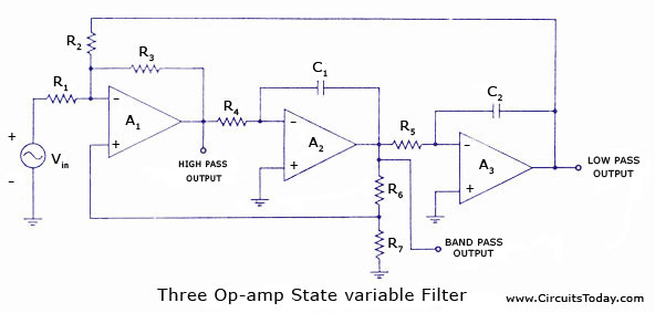
A schematic of a three op-amp, unity gain state variable filter is depicted in figure. Op-amps A₂ and A₃ are integrators while op-amp .A₁ sums the input with the low-pass output and a portion of the bandpass output. The circuit is actually a small analog com­puter designed to solve the differential equation (transfer function) for each filter type.

For proper operation Rj = R₂ = R₃ = R; R₄ = R₅ = R,; and C_x = C₂ = C.

The critical frequencies of each of the three filters are equal and is as given as

The damping is set by R₆ and R7. This determines the types of low-pass and high-pass responses (Bessel, Butterworth, or Chebyshev)

α = 3 [R₇ / R₆+R₇]

It also sets the Q and the gain of the bandpass filter

Q = 1/ α and A_band._pass = Q

The state variable filter produces the standard second-order low-pass band-pass, and high-pass responses. The critical frequencies of each are equal, and the damping is set by the feedback from the bandpass out­put. For all three outputs this damp­ing has precisely the same effect (at the same numerical values) as it did for the single op-amp filters. For low-pass and high-pass, the damp­ing coefficient of 1.414 provides a Butterworth response. Damping of 1.732 provides Bessel response, and α = 0.766 causes 3 db peaks (Chebyshev). The high-pass – 3 db frequencies are similarly shifted by the high-pass correction factor k_hp = 1/k_lp

For the band-pass section, changing the damping coefficient inversely alters the Q and gain (at critical frequency).

But the critical frequency is set by Rf and C. It is not altered by changes in the damping coefficient. This means that changes in damping only (and directly) affect the BW. So tuning of bandpass filter is very convenient. Resistor R adjusts the centre frequency only. Resistors R_A and R_B adjusts the BW only.

At this point, it is critical that we realize that optimum performance from all three outputs cannot be obtained simultaneously. For instance if we want maximum flatness in the passbands of low-pass and high-pass outputs, we must select a Butterworth response with α = 1.414. But a damping coefficient of 1.414 gives a Q and A_f of 0.707 each. The bandpass filter will not be very selective and will attenuate even the centre frequency by 30%.

On the other hand, if Q is selected to be 20 to achieve reasonable selectivity and centre-frequency gain, the low-pass and high-pass outputs will have a damping coefficient of 0.05. This will cause a pass band peak of over 25 db. We can either optimize the bandpass output or the low-pass and high-pass outputs.

NASA Robots

NASA has innovated and designed special robots which can aid them in doing tasks in dangerous environments. The most common works that are done by these robots are the repair of radiation exposed machines, capturing videos in outer space, getting into minute places inside the space craft where astronauts cannot enter and so on. In some cases, the researchers in NASA have even created robots that almost resemble to human beings in the physical structure and also the different degrees of freedom.

Some of the robots that were designed by NASA are described below.

• Robonaut

Robonaut is a robot that resembles to a human being in physical appearance. This prototype was developed in Houston, Texas by the Dextrous Robotics Laboratory at NASA’s Johnson Space Center (JSC). The main idea in creating such a robot was to help and work alongside with astronauts in space. This robot does not have the abilities to lift heavy objects and shift them. But they sure have the skills and grace in physical movement, especially in the movement of hands. Thus, Robonaut is said to be the cleverest than any other robot NASA has ever developed.

Design of Robonaut

The first design of the robot was intended for it to be used as an end-effectors for the robotic arm on the International Space Station. Thus the robot could help in all the maintenance in the external premises of the station. The robot easily became an alternative to human extravehicular activity.

The first prototypes of the robots were named R1A and R1B and had many working partners including DARPA [The Defence Advanced Research Projects Agency]. After its huge success, the second series was released and had the joint partnership of NASA and General Motors.

As time passed, Robonauts were further developed so that they could be used for teleoperation on planetary surfaces. In such operations the Robonaut would explore a planetary surface while receiving instructions from orbiting astronauts above.

Latest Robonaut – R2

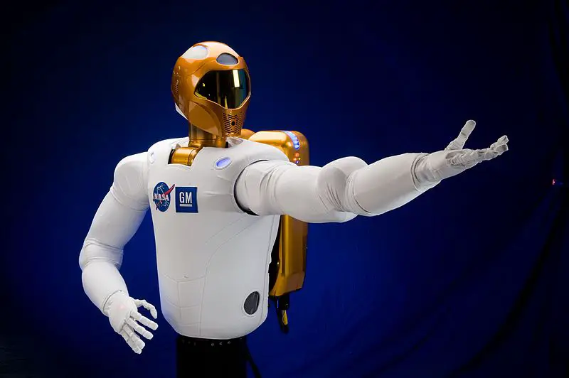
The latest version of Roboanut was named R2. The researchers are still developing it and have decided to launch it on February 24th, 2011 in the space shuttle Discovery on mission STS-133.

This robot is so advanced that it can raise its arm to almost 2 meters in one second and has 40lbs payload capacity. The robot has altogether 350 sensors and is said to have a grasping force of 5lbs. The other features of the robot are explained below.

• The hand has 12 DOF [degrees of freedom] and 2 DOF in wrist.
• Uses the highest levels of robot autonomy including telepresence.
• Has touch sensors at the tips of its fingers.
• Weighs almost 330 pounds. Has a head, a torso, 2 hands and 2 arms.

Anthropomimetic Machines

The Robotics technology has become highly advanced to such a level that even people who have routine jobs [in industries] are replaced by robots. Though the initial cost of such robots may be high, the overall gain will be huge when compared to manual labour.  To us, robots are just machines with two arms and two legs which are connected together by nuts and bolts.

Just when we were thinking that the robots were restricted to a routine job, came the invention of a new class which could even respond mentally. Today, we are going to discuss about such a class, usually referred to as Anthropomimetic Machines.

What is an Anthropomimetic Machine?

An anthropomimetic robot is a machine that can exhibit almost all kinds of human behaviour. By human behaviour, we do not mean only the external behaviour, but also internal. That is, the robot can react and act accordingly to different stimuli like human beings. Thus, this technology is sure to reduce the gap between humans and robots.

Working of Anthropomimetic Machines

• External Behaviour

For a robot to have an efficient movement and flexibility, it is necessary that the make of it should be of high standards. Thus, an Anthropomimetic Machine is made up of a material called thermoplastic polymer as it is the best material for making artificial skeletons. This material is special as it turns to liquid in a hot state and will return to a glassy state when it is cooled. Such a material is used as they mould into a desired shape after they melt and later freeze. With this method, the robot can easily attain all the degrees of freedom [DOF] easily.

The human body has tendons which are used to connect between the bones and the muscles. In a similar fashion the thermoplastic polymer acts as the robot’s tendons and corresponds to the muscles and kitelines of the robot’s body. Thus, the thermoplastic polymer can be defined as an actuator which helps in attaining all the degrees of freedom [DOF] for the robot.

The above explanation clearly defines the external appearance and movement of the robot. Now, let us discuss the internal characteristics.

• Internal Characteristics

By internal behaviour, we mean that the robot will be able to respond to different stimuli like a human being.  This can be done only by creating some basic cognitive characteristics.

For instance, if the robot has stepped on something that is not stable for it, the robot has to do the necessary corrections. This can be done only with the help of some rudimentary sensory-motor controls. Through this control, the motor will start developing ways to develop some form of intelligence. The memory will be developed in its course that after a while when the robot faces a similar obstacle, it will remember the previous incident and do the necessary steps for its survival.

About CRONOS

CRONOS is an advanced version of an anthropomimetic machine which was developed to create an illusion of interacting with humans. It was developed by Rob Knight and Owen Holland for the Machine Consciousness Lab run by the universities of Bristol and Sussex. For the full scale version of this robot, the anthropomimetic machine had to be upgraded with many computers and other sensors.

The researchers at the Essex Campus of Bristol University explained that CRONOS was a prototype actually used for the design study used for investigating materials, actuators, joints, and morphology. After developing the prototype successfully, they built a second version with a much more stable skeletal structure ad high power motors, called CRONOS 2. This robot can not only imitate the motions and stimulations of a human but can also imitate the actual external appearance of a human.

 

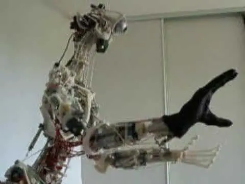
The structure of such a system is perfect that it can easily attain 42 degrees of freedom [DOF] with the help of elastically driven actuators.

CRONOS was made from nothing else but common elements like nuts, bolts, screws, actuators and so on. But CRONOS 2 was a little more advanced as the skeletal structure had to be made stronger. Thus, they made it out of thermoplastic polymorph, tendons of kiteline and so on. The muscles were designed and powered with the help of actuated screwdriver motors. The flexible joints of the muscle and bones were made out of bungee cord. These changes from the prototype to CRONOS 2 made it more identical to an actual human being, when referred to the shape and size.

Future of Anthropomimetic Robots

All these efforts were done to somehow integrating robots into human society. Anthropomimetic Robots and its versions may have succeeded in imitating and responding to human beings with the help of multiple computers and other devices. But, with major funding and research, this idea can be taken to the next level, where all the works that a human does can be done by a robot as well.

Applications

When a certain technology is innovated, they will be used for only two basic purposes. They are – good or evil. The good thing about such machines is that they can be replaced for existing technologies like ATM’s, advanced computing processes, and so on. They can also be used for bomb removal purposes. But, the bad thing is that they can replace human jobs like library assistants, grocery checkout clerks and so on. Though the researchers developed such a robot to integrate with a society, only time can tell how bad the technology can get.

Remote controlled 

appliance switch that can ON or OFF any appliance connected to it using a TV remote.

 IR remote sensor IC TSOP 1738 is used for recieving the signal. Normally when no signal is falling on IC3 the output of it will be high.This makes Q1 OFF.When a signal of 38 KHz from the TV remote falls on the IC3 its output goes low.This makes Q1 conduct and a negative pulse is obtained at pin 2 of IC 1  NE 555.Due to this IC1 wired as a monostable multivibrator produces a 4 Sec  long high signal at its out put.This high out put is the clock for IC 2 which is wired as a Flipflop and of , its two outputs pin 3 goes low and pin 2 goes high.The high output at pin 2 is amplified to drive the relay .For the next signal  the outputs of IC2 toggles state. Result, we get a relay toggling on each press on the remote.Any appliance connected to this circuit can be switched ON or OFF.

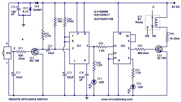
Notes.

• Before wiring the circuit make sure that the carrier frequency  of the TV remote you have is 38 KHz.For that wire the sensor part only ,point your remote to the TSOP1738 and press any switch.If  out put of TSOP1738  goes  low them ok, your remote is of 38Khz type.Nothing to worry almost all TV remote are of this type.
• You can use any switch because for any switch the code only changes,the carrier frequency remains same.We need this carrier frequency only.
• Assemble the circuit on a good quality PCB or common board.
• The appliance can be connected through NO or NC  and contacts of the relay . 

                       

Traffic Lights using 4017 & 555 Timer

traffic light system. Which operates for 1-7 minutes by adjusting 1M potentiometer.

555 timer behaves as a clock pulse generator which is input to binary counter having outputs Q0 – Q9.

Appropriate outputs are combined with diodes to on/off the particular LEDs.

Parts Required: 330R, 22k, 100k 1M Potentiometer 0.1μF, 10μF, 2.2mF 1N4148 x (6) Red, Yellow and green LEDs 555 timer IC 4017 counter IC 9V Battery

Circut Diagram:

                                Electronic Control Systems                                       

                        Model and Remote Control schematics                         

                               Flying Robot Circuit Diagram                                

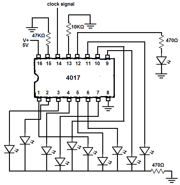
           XO___XO DW  Electronic Control Systems: Basic (Energy Engineering)            

Every piece of energy-consuming equipment has some form of control system associated with it. This article provides information about electronic control systems primarily used to control HVAC equipment. The same principles are used to control other equipment, such as lighting, compressed air systems, process equipment, and production equipment.

INTRODUCTION

Every piece of energy-consuming equipment has some form of control system associated with it. The controls can be as simple as a snap switch or as complicated as a dedicated microcomputer chip system. Larger pieces of equipment, along with buildings and industrial processes, typically use complex computer-based control systems to optimally control and operate them. This article provides information about electronic control systems primarily used to control HVAC equipment. However, the same technologies and principles are used to control other equipment, such as lighting, compressed air systems, process equipment and production equipment.

An electronic control system comprises a sensor, controller and final control element. The sensors used in electronic control systems are simple, low-mass devices that provide stable, wide-range, linear and fast response. The electronic controller is a solid-state device that provides control over a discrete portion of the sensor range and generates an amplified correction signal to control the final control element.

Features of electronic control systems include the following:

• Controllers can be remotely located from sensors and actuators.

• Controllers can accept a variety of inputs.

• Remote adjustments for multiple controls can be located together, even though sensors and actuators are not.

• Electronic control systems can accommodate complex control and override schemes.

• Universal type outputs can interface to many different actuators.

• Display meters can indicate input or output values.

The sensors and output devices (e.g., actuators, relays) used for electronic control systems are usually the same ones used on microprocessor-based systems. The distinction between electronic control systems and microprocessor-based systems is in the handling of the input signals. In an electronic control system, the analog sensor signal is amplified, then compared to a setpoint or override signal through voltage or current comparison and control circuits. In a microprocessor-based system, the sensor input is converted to a digital form, in which discrete instructions (algorithms) perform the process of comparison and control.

Fig. 1 shows a simple electronic control system with a controller that regulates supply water temperature by mixing return water with water from the boiler. The main temperature sensor is located in the hot water supply from the valve. To increase efficiency and energy savings, the controller resets the supply water temperature setpoint as a function of the OA (outdoor air) temperature. The controller analyzes the sensor data and sends a signal to the valve actuator to regulate the mixture of hot water to the unit heaters. These components are described in the section titled “Components.”

A glossary of control system terms is given in the last section of this article.

Electronic control systems usually have the following characteristics:

Controller. Low voltage, solid state. Inputs. 0-1 V d.c., 0-10 V d.c., 4-20 mA, resistance element, thermistor, thermocouple. Outputs. 2-10 V d.c. or 4-20 mA device. Control Mode. Two-position, proportional, proportional plus integral (PI) or step.

Fig. 1 Basic electronic control system.

Circuit diagrams in this article are basic and fairly general. A resistance-temperature input and a 2-10 V d.c. output are used for purposes of discussion. A detailed discussion on control modes can be found in the “Control Fundamentals” section of the Engineering Manual of Automatic Controls.[1]

ELECTRONIC CONTROL SYSTEM COMPONENTS

An electronic control system includes sensors, controllers, output devices such as actuators and relays; final control elements such as valves and dampers; and indicating, interfacing, and accessory devices. Fig. 2 provides a system overview for many electronic system components.

Sensors

A sensing element provides a controller with information concerning changing conditions. Analog sensors are used to monitor continuously changing conditions such as temperature or pressure. The analog sensor provides the controller with a varying signal such as 0-10 V. A digital (two-position) sensor is used if the conditions represent a fixed state such as a pump that is on or off. The digital sensor provides the controller with a discrete signal such as open or closed contacts.

Fig. 2 Typical electronic control system components.

Some electronic sensors use an inherent attribute of their material (e.g., wire resistance) to provide a signal and can be directly connected to the electronic controller. Other sensors require conversion of the sensor signal to a type or level that can be used by the electronic controller. For example, a sensor that detects pressure requires a transducer or transmitter to convert the pressure signal to a voltage that can be used by the electronic controller. Typical sensors used in electronic control systems are included in Fig. 2. A sensor-transducer assembly is called a transmitter.

Temperature Sensors

For electronic control, temperature sensors are classified as follows:

• Resistance temperature devices (RTDs) change resistance with varying temperature. RTDs have a positive temperature coefficient (resistance increases with temperature).

• Thermistors are solid-state resistance-temperature sensors with a negative temperature coefficient.

• Thermocouples directly generate a voltage as a function of temperature.

Resistance Temperature Devices

In general, all RTDs have some common attributes and limitations:

• The resistance of RTD elements varies as a function of temperature. Some elements exhibit large resistance changes, linear changes, or both over wide temperature ranges.

• The controller must provide some power to the sensor and measure the varying voltage across the element to determine the resistance of the sensor. This action can cause the element to heat slightly—called self-heating—and can create an inaccuracy in the temperature measurement. By reducing the supply current or by using elements with higher nominal resistances, the self-heating effect can be minimized.

• Some RTD element resistances are as low as 100 Q. In these cases, the resistance of the lead wires connecting the RTD to the controller may add significantly to the total resistance of the connected RTD, and can create an offset error in the measurement of the temperature. Fig. 3 shows a sensor and controller in relation to wire lead lengths. In this figure, a sensor 25 ft from the controller requires 50 ft of wire. If 18 AWG solid copper wire with a d.c. resistance of 6.39 Q/Mft is used, the 50 ft of wire has a total d.c. resistance of 0.319 Q. If the sensor is a 100-ohm platinum sensor with a temperature coefficient of 0.69 Q/°F, the 50 ft of wire will introduce an error of 0.46°F. If the sensor is a 3000-ohm platinum sensor with a temperature coefficient of 4.8 Q/°F, the 50 ft of wire will introduce an error of 0.066°F.

Fig. 3 Lead wire length.

Significant errors can be removed by adjusting a calibration setting on the controller, or—if the controller is designed for it—a third wire can be run to the sensor and connected to a special compensating circuit designed to remove the lead length effect on the measurement. In early electronic controllers, this three-wire circuit was connected to a Wheatstone Bridge configured for lead wire compensation. In digital controllers, lead wire compensation on low resistance sensors may be handled by software offset.

• The usable temperature range for a given RTD sensor may be limited by non-linearity at very high or low temperatures.

• RTD elements that provide large resistance changes per degree of temperature reduce the sensitivity and complexity of any electronic input circuit. (Linearity may be a concern, however.)

A sensor constructed using a BALCO wire is a commonly used RTD sensor. BALCO is an annealed resistance alloy with a nominal composition of 70 percent nickel and 30 percent iron. A BALCO 500-ohm resistance element provides a relatively linear resistance variation from — 40 to 250°F. The sensor is a low-mass device and responds quickly to changes in temperature.

Another material used in RTD sensors is platinum. It is linear in response and stable over time. In some applications, a short length of wire is used to provide a nominal resistance of 100 Q. However, with a low resistance value, the element can be affected by self-heating and sensor-leadwire resistance. Additionally, due to the small amount of resistance change of the element, additional amplification must be used to increase the signal level.

To use the desirable characteristics of platinum and minimize any offset, one manufacturing technique deposits a film of platinum in a ladder pattern on an insulating base. A laser trimming method (Fig. 4) then burns away a portion of the metal to calibrate the sensor, providing a resistance of 1000 Q at 74°F. This platinum film sensor provides a high resistance-to-temperature relationship. With its high resistance, the sensor is relatively immune to self-heating and sensor-leadwire resistance offsets. In addition, the sensor is an extremely low-mass device and responds quickly to changes in temperature. RTD elements of this type are common.

 Fig.

Fig. 4 Platinum element RTD sensor.

Solid-State Resistance Temperature Devices

Fig. 5 shows examples of solid-state resistance temperature sensors having negative and positive temperature coefficients. Thermistors are negative temperature coefficient sensors typically enclosed in very small cases (similar to glass diodes or small transistors) that provide quick response. As the temperature increases, the resistance of a thermistor decreases (Fig. 6). Selection of a thermistor sensor must consider the highly nonlinear temperature-resistance characteristic.

Fig. 5 Solid-state temperature sensors.

Positive temperature coefficient solid-state temperature sensors may have relatively high resistance values at room temperature. As the temperature increases, the resistance of the sensor increases (Fig. 6). Some solid-state sensors have near-perfect linear characteristics over their usable temperature range.

Thermocouples

In a thermocouple, two dissimilar metals such as iron and constantan are welded together to form a thermocouple junction (Fig. 7). When this junction is exposed to heat, a voltage in the millivolt range is generated and can be measured by the input circuits of an electronic controller. The amount of voltage generated is directly proportional to the temperature (Fig. 8). At room temperatures for typical HVAC applications, these voltage levels are often too small to be used, but are more usable at higher temperatures of 200°F-1600°F. Consequently, thermocouples are most common in high-temperature process applications.

Transmitter/Transducer

The input circuits for many electronic controllers can accept a voltage range of 0-10 V d.c. or a current range of 4-20 mA. The inputs to these controllers are classified as universal inputs because they accept any sensor having the correct output. These sensors are often referred to as transmitters as their outputs are an amplified or conditioned signal. The primary requirement of these transmitters is that they produce the required voltage or current level for an input to a controller over the desired sensing range.

Transmitters measure various conditions such as temperature, relative humidity, airflow, water flow, power consumption, air velocity and light intensity. An example of a transmitter would be a sensor that measures the level of carbon dioxide (CO2) in the return air of an air handling unit. The sensor provides a 4-20 mA signal to a controller input, which can then modulate outdoor/exhaust dampers to maintain acceptable air quality levels. Since electronic controllers are capable of handling voltage, amperage or resistance inputs, temperature transmitters are not usually used as controller inputs within the ranges of HVAC systems due to their high cost.

Relative Humidity Sensor

Various sensing methods are used to determine the percentage of relative humidity, including the measurement of changes of resistance, capacitance, impedance and frequency.

An older method that used resistance to determine relative humidity depended on a layer of hygroscopic salt, such as lithium chloride or carbon powder, deposited between two electrodes (Fig. 9). Both materials absorb and release moisture as a function of the relative humidity, causing a change in resistance of the sensor. An electronic controller connected to this sensor detects the changes in resistance, which it can use to provide control of relative humidity.

A method that uses changes in capacitance to determine relative humidity measures the capacitance between two conductive plates separated by a moisture-sensitive material such as polymer plastic (Fig. 10A). As the material absorbs water, the capacitance between the plates decreases, and the change can be detected by an electronic circuit. To overcome any hindrance of the material’s ability to absorb and release moisture, the two plates and their electric leadwires can be on one side of the polymer plastic, with a third sheet of extremely thin conductive material on the other side of the polymer plastic forming the capacitor (Fig. 10B). This third plate, too thin for attachment of leadwires, allows moisture to penetrate and be absorbed by the polymer, thus increasing sensitivity and response.

A relative humidity sensor that generates changes in both resistance and capacitance to measure moisture level is constructed by anodizing an aluminum strip and then applying a thin layer of gold or aluminum (Fig. 11). The anodized aluminum has a layer of porous oxide on its surface. Moisture can penetrate through the gold layer and fill the pores of the oxide coating, causing changes in both resistance and capacitance that can be measured by an electronic circuit.

Sensors that use changes in frequency to measure relative humidity (Fig. 12) can use a quartz crystal coated with a hygroscopic material such as polymer plastic. When the quartz crystal is energized by an oscillating circuit, it generates a constant frequency. As the polymer material absorbs moisture and changes the mass of the quartz crystal, the frequency of oscillation varies and can be measured by an electronic circuit.

Most relative humidity sensors require electronics at the sensor to modify and amplify the weak signal and are referred to as transmitters. The electronic circuit compensates for the effects of temperature and both amplifies and linearizes the measured level of relative humidity. The transmitters typically provide a voltage or current output that can be used as an input to the electronic controller.

Pressure Sensors

An electronic pressure sensor converts pressure changes into a signal such as voltage, current or resistance that can be used by an electronic controller.

A method that measures pressure by detecting changes in resistance uses a small, flexible diaphragm and a strain gage assembly (Fig. 13). The strain gage assembly includes very fine (serpentine) wire or a thin metallic film deposited on a nonconductive base. The strain gage assembly is stretched or compressed as the diaphragm flexes with pressure variations. The stretching or compressing of the strain gage (shown by a dotted line in Fig. 13) changes the length of its fine wire or thin film metal, which changes the total resistance. The resistance can then be detected and amplified. These changes in resistance are small. Therefore, an amplifier is provided in the sensor assembly to amplify and condition the signal so the level sent to the controller is less susceptible to external noise interference. The sensor thus becomes a transmitter.

Fig. 10 Capacitance-type relative humidity sensor.

Fig. 11 Impedance-type relative humidity sensor.

Another pressure sensing method measures capacitance (Fig. 14). A fixed plate forms one part of the capacitor assembly, and a flexible plate is the other part of the capacitor assembly. As the diaphragm flexes with pressure variations, the flexible plate of the capacitor assembly moves closer to the fixed plate (shown by a dotted line in Fig. 14) and changes the capacitance.

A variation of pressure sensors is one that measures differential pressure using dual pressure chambers (Fig. 15). The force from each chamber acts in an opposite direction with respect to the strain gage. This type of sensor can measure small differential pressure changes even with high static pressure.

Controllers, Output Devices and Indicating Devices

Controller

The electronic controller receives a sensor signal, amplifies and/or conditions it, compares it with the setpoint, and derives a correction if necessary. The output signal typically positions an actuator. Electronic controller circuits allow a wide variety of control functions and sequences, from very simple arrangements to multiple-input circuits with several sequential outputs. Controller circuits use solid-state components, such as transistors, diodes and integrated circuits, and include the power supply and all the adjustments required for proper control.

Fig. 12 Quartz crystal relative humidity sensor.

Fig. 13 Resistance-type pressure sensor.

Input Types

Electronic controllers are categorized by the type or types of inputs they accept, such as temperature, humidity, enthalpy or universal.

Temperature Controllers

Temperature controllers typically require a specific type or category of input sensors. Some have input circuits to

Fig. 14 Capacitance-type pressure transmitters.

accept RTD sensors such as BALCO or platinum elements, while others contain input circuits for thermistor sensors. These controllers have setpoint and throttling range scales labeled in degrees Fahrenheit or Celsius.

Relative Humidity Controllers

The input circuits for relative humidity controllers typically receive the sensed relative humidity signal already converted to a 0-10 V d.c. voltage, or a 4-20 mA current signal. Setpoint and scales for these controllers are in percent relative humidity.

Fig. 15 Differential pressure sensor.

Enthalpy Controllers

Enthalpy controllers are specialized devices that use specific sensors for inputs. In some cases, the sensor may combine temperature and humidity measurements and convert them to a single voltage to represent enthalpy of the sensed air. In other cases, individual dry-bulb temperature sensors and separate wet-bulb or relative humidity sensors provide inputs, and the controller calculates enthalpy. In typical applications, the enthalpy controller provides an output signal based on a comparison of two enthalpy measurements, indoor and outdoor, rather than on the actual enthalpy value. In other cases, the return air enthalpy is assumed constant so that only OA enthalpy is measured. It is compared against the assumed nominal return air value.

Universal Controllers

The input circuits of universal controllers can accept one or more of the standard transmitter or transducer signals. The most common input ranges are 0-10 V d.c. and 4-20 mA. Other input variations in this category include a 2-10 V d.c. and a 0-20 mA signal. Because these inputs can represent a variety of sensed variables, such as a current of 0-15 A or pressure of 0-3000 psi, the settings and scales are often expressed in percent of full scale only.

Control Modes

The control modes of some electronic controllers can be selected to suit the application requirements. Control modes include two-position, proportional and proportional-integral. Other control features include remote setpoint, the addition of a compensation sensor for reset capability, and override or limit control.

Output Control

Electronic controllers provide outputs to a relay or actuator for the final control element. The output is not dependent on the input types or control method. The simplest form of output is two-position, in which the final control element can be in one of two states. For example, an exhaust fan in a mechanical room can be turned either on or off. The most common output form, however, provides a modulating output signal which can adjust the final control device (actuator) between 0 and 100 %, such as in the control of a chilled water valve.

Fig. 16 Two-position control.

Output Devices

Actuators, relays, and transducers (Fig. 2) are output devices which use the controller output signal (voltage, current, or relay contact) to perform a physical function on the final control element such as starting a fan or modulating a valve. Actuators can be categorized as devices that provide two-position action or as those that provide modulating action.

Two-Position

Two-position devices such as relays, motor starters, and solenoid valves have only two discrete states. These devices interface between the controller and the final control element. For example, when a solenoid valve is energized, it allows steam to enter a coil that heats a room (Fig. 16). The solenoid valve provides the final action on the controlled media, steam. Damper actuators can also be designed to be two-position devices.

Modulating

Modulating actuators use a varying control signal to adjust the final control element. For example, a modulating valve controls the amount of chilled water entering a coil so that cool supply air is just sufficient to match the load at a desired setpoint (Fig. 17). The most common modulating actuators accept a varying voltage input of 0-10 V, or 2-10 V d.c., or a current input of 4-20 mA. Another form of actuator requires a pulsating (intermittent) or duty cycling signal to perform modulating functions. One form of pulsating signal is a Pulse Width Modulation (PWM) signal.

Fig. 17 Modulating control.

Fig. 18 Electric-to-pneumatic transducer.

Tranducer

In some applications, a transducer converts a controller output to a signal that is usable by the actuator. For example, Fig. 18 shows an Electronic-to-Pneumatic (E/P) transducer that converts a modulating 2-10 V d.c. signal from the electronic controller to a pneumatic proportional modulating 3-13 psi signal for a pneumatic actuator.

Indicating Devices

An electronic control system can be enhanced with visual displays that show system status and operation. Many electronic controllers have built-in indicators that show power, input signal, deviation signal and output signal. Fig. 19 shows some types of visual displays. An indicator light can show on/off status or, if driven by controller circuits, the brightness of a light can show the relative strength of a signal. If a system requires an analog or digital indicating device and the electronic controller does not include this type of display, separate indicating devices can be provided.

Interface with Other Systems

It is often necessary to interface an electronic control device to a microprocessor-based building management system or other related system. An example is an interface that allows a building management system to adjust the setpoint or amount of reset (compensation) for a specific controller. Compatibility of the two systems must be verified before they are interconnected.

Fig. 19 Indicating devices.

ELECTRONIC CONTROLLER FUNDAMENTALS

General

The electronic controller is the basis for an electronic control system. Fig. 20 shows the basic circuits of an electronic controller including power supply, input, control and output. For greater stability and control, internal feedback correction circuits also can be included, but these are not discussed here. The circuits described provide an overview of the types and methods of electronic controllers.

Power Supply Circuit

The power supply circuit of an electronic controller provides the required voltages to the input, control, and output circuits. Most voltages are regulated DC voltages. The controller design dictates the voltages and current levels required.

All power supply circuits are designed to optimize both line and load regulation requirements within the needs and constraints of the system. Load regulation refers to the ability of the power supply to maintain the voltage output at a constant value even as the current demand (load) changes. Similarly, line regulation refers to the ability of the power supply to maintain the output load voltage at a constant value when the input (AC) power varies. The line regulation abilities or limitations of a controller are usually part of the controller specifications such as 120 V AC + 10%, -15%. The degree of load regulation involves the end-to-end accuracy and repeatability, and is usually not explicitly stated as a specification for controllers.

TYPICAL SYSTEM APPLICATIONS

Fig. 21 shows a typical air-handling system controlled by two electronic controllers, C1 and C2; sequencer S; multi-compensator M; temperature sensors T1 through T4; modulating hot- and chilled-water valves V1 and V2; and outdoor, return, and exhaust air damper actuators. The control sequence is as follows:

• Controller C1 provides outdoor compensated, summer/ winter control of space temperature for a heating/ cooling system which requires PI control with a low limit. Sensor T4 provides the compensation signal through multi-compensator M, which allows one outdoor temperature sensor to provide a common input to several controllers. Controller C1 modulates the hot-and chilled-water valves V1 and V2 in sequence to maintain space temperature measured by sensor T1 at a pre-selected setpoint. Sequencer S allows sequencing the two valve actuators from a single controller. Low-limit sensor T2 assumes control when the discharge air temperature drops to the control range of the low-limit setpoint. A minimum discharge air temperature is maintained regardless of space temperature.

Fig. 20 Electronic controller circuits.

When the outdoor temperature is below the selected reset changeover point set on C1, the controller is in the winter compensation mode. As the outdoor air temperature falls, the space temperature setpoint is raised. When the outdoor temperature is above the reset changeover point, the controller is in the summer compensation mode. As the outdoor temperature rises, the space temperature setpoint is raised.

• Controller C2 provides PI mixed air temperature control with economizer operation. When the OA temperature measured by sensor T4 is below the setting of the economizer startpoint setting, the controller provides proportional control of the dampers to maintain mixed air temperature measured by sensor T3 at the selected setpoint. When the OA temperature is above the economizer startpoint setting, the controller closes the OA dampers to a preset minimum.

Fig. 21 Typical application with electronic controllers.

ADDITIONAL DEFINITIONS

Authority (reset authority or compensation authority). A setting that indicates the relative effect a compensation sensor input has on the main setpoint (expressed in percent).

Compensation change-over. The point at which the compensation effect is reversed in action and changes from summer to winter or vice versa. The percent of compensation effect (authority) may also be changed at the same time.

Control Point. The actual value of a controlled variable (setpoint plus or minus offset).

Deviation. The difference between the setpoint and the value of the controlled variable at any moment. Also called “offset.”

Direct acting. A direct-acting controller increases its output signal on an increase in input signal.

Electric control. A control circuit that operates on line or low voltage, and uses a mechanical means, such as a temperature-sensitive bimetal or bellows, to perform control functions, such as actuating a switch or positioning a potentiometer. The controller signal usually operates or positions an electric actuator, although relays and switches are often controlled.

Electronic control. A control circuit that operates on low voltage and uses solid-state components to amplify input signals and perform control functions, such as operating a relay or providing an output signal to position an actuator. Electronic devices are primarily used as sensors. The controller usually furnishes fixed control routines based on the logic of the solid-state components.

Electronic controller. A solid-state device usually consisting of a power supply, a sensor amplification circuit, a process/comparing circuit, an output driver section, and various components that sense changes in the controlled variable and derive a control output which provides a specific control function. In general, adjustments such as setpoint and throttling range necessary for the process can be done at the controller via potentiometers and/or switches.

Final control element. A device such as a valve or damper that changes the value of the manipulated variable. The final control element is positioned by an actuator.

Integral action (I). An action in which there is a continuous linear relationship between the amount of increase (or decrease) on the output to the final control element and the deviation of the controlled variable to reduce or eliminate the deviation or offset.

Limit sensor. A device which senses a variable that may be other than the controlled variable and overrides the main sensor at a preset limit.

Main sensor. A device or component that measures the variable to be controlled.

Negative (reverse) reset. A compensating action in which a decrease in the compensation variable has the same effect as an increase in the controlled variable. For example, in a heating application, as the outdoor air temperature decreases, the control point of the controlled variable increases. Also called “winter reset or compensation.”

Offset. A sustained deviation between the control point and the setpoint of a proportional control system under stable operating conditions. Also called “deviation.”

Positive (direct) reset. A compensating action in which an increase in the compensation variable has the same effect as an increase in the controlled variable. For example, in a cooling application, as the OA temperature increases, the control point of the controlled variable increases. Also called “summer reset or compensation.”

Proportional band (throttling range). In a proportional controller, the control point range through which the controlled variable must pass to drive the final control element through its full operating range. Proportional band is expressed in percent of the main sensor span. A commonly used equivalent is “throttling range,” which is expressed in values of the controlled variable.

Proportional control (P). A control algorithm or method in which the final control element moves to a position proportional to the deviation of the value of the controlled variable from the setpoint.

Proportional-integral (PI) control. A control algorithm that combines the proportional (proportional response) and integral or deviation control algorithms. Integral action tends to correct the offset resulting from proportional control. Also called “proportional plus reset” or “two-mode” control.

Remote setpoint. A means for adjusting the controller setpoint from a remote location, in lieu of adjusting it at the controller itself. The means of adjustment may be manual with a panel or space mounted potentiometer, or automatic when a separate device provides a signal (voltage or resistive) to the controller.

Reset control. A process of automatically adjusting the control point of a given controller to compensate for changes in a second measured variable such as outdoor air temperature. For example, the hot deck control point is reset upward as the outdoor air temperature decreases. Also known as “compensation control.”

Reset sensor. The system element which senses a variable other than the controlled variable and resets the main sensor control point. The amount of this effect is established by the authority setting.

Reverse acting. A reverse-acting controller decreases its output signal on an increase in input signal.

Setpoint. The value on the controller scale at which the controller is set, such as the desired room temperature set on a thermostat. The setpoint is always referenced to the main sensor (not the reset sensor).

Throttling range. In a proportional controller, the control point range through which the controlled variable must pass to move the final control element through its full operating range. Throttling range is expressed in values of the controlled variable such as temperature in degrees Fahrenheit, relative humidity in percent, or pressure in pounds per square inch. A commonly used equivalent is “proportional band,” which is expressed in percent of sensor span for electronic controls.

Transducer. A device that converts one energy form to another. It amplifies (or reduces) a signal so that the output of a sensor or transducer is usable as an input to a controller or actuator. A transducer can convert a pneumatic signal to an electric signal (P/E transducer) or vice versa (E/P transducer), or it can convert a change in capacitance to an electrical signal.

Transmitter. A device that converts a sensor signal to an input signal usable by a controller or display device.

CONCLUSION

Basic automatic electronic control systems are extremely important to provide desirable operational features of energy-using equipment and systems. Proper control is critical to achieving functional performance, as well as energy-efficient performance in equipment, buildings and processes.

++++++++++++++++++++++++++++++++++++++++++++++++++++++++++++++++++++++++++

                                                       e- Control DIREW                                                

       

++++++++++++++++++++++++++++++++++++++++++++++++++++++++++++++++++++++++++