
Audio Mixer with Multiple Controls
When recording sound from several orchestral instruments being
played by different musicians using a single microphone, the only way to adjust
the sound balance is to change the position of the musicians relative to the
microphone. When recording direct to stereo master tape, it’s crucial to make
sure that all the voices and instruments sound right before you hit the record
button. Presented here is an eight-input audio mixer circuit with bass, treble,
volume and balance controls, which you can use to balance sounds from all the
sources until you have the desired mix. For capturing the sound from various
sources, the audio mixer employs up to eight microphones.


Audio mixer circuit
Fig. 1 shows the block diagram of the audio mixing system along
with the audio power
amplifier, while the circuit of the audio mixer along with tone
controller is shown in Fig. 2. The power supply and audio power amplifier
circuits are shown in Figs 3 and 4, respectively.
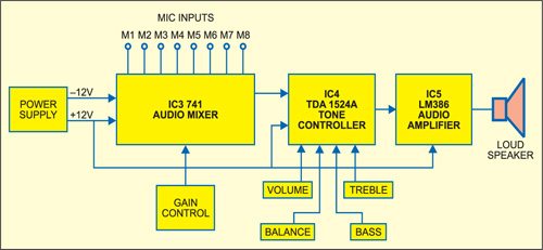
Here, dual operational amplifier IC 747 (IC3) is used for mixing
several inputs without any mutual interaction. The two internal amplifiers
share a common bias network and power supply. The IC has short-circuit
protection and wide common-mode and differential voltage ranges.
In this application, +12V and –12V regulated DC supplies are
used for operation of IC 747. The microphone output signals M1 through M4,
after their individual level adjustments, are mixed and applied across the
differential input terminals (pins 1 and 2). Similarly, microphone outputs M5
through M8 are applied across the differential input terminals (pins 7 and 6)
of the second amplifier inside op-amp IC 747 after their individual level
adjustments.
Circuit operation
For level adjustment, logarithmic variable resistors VR1 through
VR4 and VR5 through VR8, respectively, are employed while feeding the output
from respective microphones to the input of the two amplifiers inside IC 747.
The outputs of the two amplifiers taken from pins 12 and 10, respectively, are
combined at the junction of resistors R9 and R10 before feeding to the next
stage (tone controller) via capacitor C12 (10 µF). The overall gain of
individual amplifiers can be adjusted with the help of potmeters VR9 and VR10,
respectively.
The amplified mixed signal output of IC 747 is applied to
shorted input pins 15 and 4 of stereo tone controller IC TDA1524A (IC4).
TDA1524A is designed as an active stereo-tone/volume control for car radios, TV
receivers and mains-fed equipment. It includes functions for bass and treble
control, volume control with built-in contour (can be switched off) and
balance. All these functions can be controlled by DC voltages or by single
linear potentiometers. This IC serves as an efficient tone controller. Although
it may work reasonably well with 9V DC supply, for better bass response, a 12V
supply can be used. A good heat-sink is necessary for longer life and better
performance of the IC.

Features of TDA1524A are:
1. Simple construction
2. Low noise and distortion
3. Switchable contour (for quick changing of the tonal response)
4. Its output can drive most power amplifiers.
5. Bass emphasis can be increased by incorporating a double-pole, low-pass filter
6. Wide power supply voltage range
1. Simple construction
2. Low noise and distortion
3. Switchable contour (for quick changing of the tonal response)
4. Its output can drive most power amplifiers.
5. Bass emphasis can be increased by incorporating a double-pole, low-pass filter
6. Wide power supply voltage range
General specifications are:
1. DC input: 12V (typical)
2. DC battery: 35 mA
3. Maximum output: 3V RMS
4. Maximum input: 2.5V
5. Maximum gain: 21.5 dB
6. Volume control range: –80 to+121.5 dB
7. THD at 1 kHz: 0.3%
8. Ripple rejection at 100 Hz: 50 dB
1. DC input: 12V (typical)
2. DC battery: 35 mA
3. Maximum output: 3V RMS
4. Maximum input: 2.5V
5. Maximum gain: 21.5 dB
6. Volume control range: –80 to+121.5 dB
7. THD at 1 kHz: 0.3%
8. Ripple rejection at 100 Hz: 50 dB
Potmeters VR11, VR12, VR13 and VR14 are meant for adjustment of
volume, balance, bass and treble, respectively. Switch S2 is contour switch,
which can be used to change the tonal response of the of the IC. The outputs
are available at pins 8 and 11 for right and left channel, respectively. (EFY
note. Since both the left- and right-channel input pins 15 and 4 have been
shorted in this application, the IC acts as a mono volume/tone control
circuit.) .
Audio power amplifier
The audio amplifier circuit shown in Fig. 4 is optional. One can
use much higher-power audio amplifier along with the audio mixer circuit.
The low-power audio amplifier employing IC LM386 (IC5) shown in
Fig. 4 can output a maximum audio power of 1 watt. It gets +12V DC supply at
its pin 6. The audio input from sources like Walkman and audio mixer can be fed
to pin 3 of IC5 through volume control VR15.
The gain of LM386 is internally set to 20 to keep the external
part count low. However, to make LM386 a more versatile amplifier, pins 1 and 8
are provided for setting the gain—externally to any value between 20 and 200—by
using an appropriate combination of a resistor and a capacitor. If only a
capacitor is put between pins 1 and 8 using switch S3 as shown in Fig. 4, the
gain would increase to 200 (46 dB). The amplified output is taken from pin 5
and fed to the loudspeaker through electrolytic capacitor C39 (100 µF). The
higher the value of C39, the higher the pitch of the audio frequency response
in the speaker.
Figure : Digital Audio
The power supply section for the circuit is shown in Fig. 3. It
consists of a step-down transformer (230V AC primary to 12V-0-12V, 1A
secondary), bridge rectifier, filter network and regulator ICs 7812 and 7912 to
provide +12V and –12V regulated DC outputs, respectively. When switch S1 is
closed, the presence of power is indicated by the glowing of LED1.
Construction
Assemble the circuit on any general-purpose PCB. Mount IC bases
on the PCB. There is no soldering method that is ideal for all IC packages. The
use of IC bases prevents damage to the ICs while soldering and also makes it
easy to replace them. Use audio input jack connectors for M1 through M8 input
points. Also use audio output connectors at the outputs of IC4.
A combined actual-size, single-side PCB layout for Figs 2 and 3
is shown in Fig. 5 and its components layout in Fig. 6. The solder-side PCB
layout for Fig. 4 is shown in Fig. 7 and its components layout in Fig. 8.
Note. If you are not using IC base for TDA1524A, the maximum
permissible temperature of the solder is 260°C; solder at this temperature must
not be in contact with the joint for more than five seconds. The total contact
time of successive solder waves must not exceed five seconds while using wave
soldering.
Testing procedure
1.
After assembling the PCB, check the circuit connections before
switching on the power supply.
2.
Use a standard microphone at the first input point M1 and then
keep it near an audio source. You can use the power amplifier circuit given
here for testing or another higher-output power amplifier.
3.
Vary VR1 slowly until a clear and distortion-free amplified
output is obtained.
4.
If the sound output is not clear and VR1 does not help, vary
gain control VR9.
5.
If the problem still persists, check volume, balance, bass and
treble controls.
6.
Check the various controls in your audio power amplifier
section.
Repeat steps 2 through 5 for the rest of the inputs. Having checked all
the inputs, now the audio mixer is ready for use .
INTRODUCTION INTO DIGITAL AUDIO, PSYCHOACOUSTICS AND MSP.
reviewing some principles of digital audio (discrete time and audio in digital systems) and discussed some basic concepts, such as the Nyquist-Shannon theorem, the meaning of word size (or bit depth), vector sizes (audio buffer sizes), and looked at the path a sound wave takes from its physical production into the digital system and after being processed its conversion back into the physical world (see figure below).
We then started producing our first sound in MSP (using the [cycle~] object), used simple arithmetics [*~], [+~] for mixing and scaling signals, and introduced objects for routing audio ([selector~], [gate~]) and sending/receiving audio signals without patch cords ([send~]/[receive~]). We then produced our discussed the properties (time domain and frequency domain) of basic waveforms, namely sine wave, sawtooth, rectangle (or square), and different types of noises.
We then went on discussing perceptual characteristics of sound perception and psychoacoustics, such as pitch perception, and experimented with distorted and stretched/compressed harmonic spectra.
XO__XO Op Amp PID Controller as like as setting program mixing
CIRCUIT
OP_PID1.CIR Download the SPICE file
We've all heard about the wonders of the PID controller, bringing a system's output - temperature, velocity, light - to its desired set point quickly and accurately. But now, your boss says okay, design one for us. Although there's a number of ways to do it, the circuit above nicely separates the three terms into three individual op amp circuits. We'll build it in SPICE, test each term and finally place it inside a motor speed controller for you to tune. If you wish, take a quick review of PID Control.THE PID CONTROLLER
What basic components are needed for a servo system? Many look similar to the circuit below. The error amp gives you a constant reality check. How? It compares where you want to go, Vset, with where you're at now, Vsensor, by calculating the difference between the two, Verr = Vset - Vsensor. The PID controller takes this error and determines the drive voltage applied to the process in an attempt to bring Vset = Vsensor or Verr = 0.
ERROR AMPLIFIER. A classic circuit for calculating the error is a summing op amp. In the controller, XOP1 performs the error calculation. Remembering that the summing amp is an inverting amp, we calculate its output using R1 = R2 = R3 = 10 kΩ.
But how does the summer calculate a difference? Well, it does require that your sensor circuit produce a negative output voltage. Assuming that Vsensor is the negative of the actual sensor voltage Vsensor = - Vsens, you get the difference.Verr = - (Vset / R1 + Vsensor / R2) ∙ R3
= (Vset + Vsensor) ∙ (10 k / 10 k)
= - ( Vset + Vsensor )
You can look at the error amp's function this way. When Vsensor is exactly the negative of Vset, the currents through R1 and R2, equal and opposite, cancel each other as they enter the op amps's summing junction. You end up with zero current through R3 and of course 0V, or zero error, at the output. Any difference between Vset and -Vsensor, results in an error voltage at the output that the PID controller can act upon.Verr = -( Vset - Vsens )
OP AMP PID CONTROLLER. How do we get the PID terms from the error voltage Verr? We enlist three simple op amp circuits. If you need, take a review of the op amp amplifier,integrator and differentiator circuits.
Lastly, we need to add the three PID terms together. Again the summing amplifier XOP5 serves us well. Because the error amp, PID and summing circuits are inverting types, we need to add a final op amp inverter XOP6 to make the final output positive, given a positive Vset.
Term Op Amp Circuit Function P Amplifier: Vo = (RP2 / RP1) ∙ Verr I Integrator: Vo = 1/(RI∙CI) ∙ ∫ Verr dt D Differentiator: Vo = RD∙CD ∙ dVerr / dt
OUTPUT PROCESS. EOUT represents a very simplified model of a process to be controlled, such as motor velocity for example. The gain of 100 could represent an output transfer function of 100 RPM / V. To include the effects of the motor's inertia, we've added some time delay into the output using two cascaded RC filters. Although Vout is simulated in volts, we know it really represents RPM.
SENSOR. The sensor tells you the actual velocity at the motor, 1 V / 100 RPM for this tachometer. ESENSOR models this feedback device. Note, this sensor block actually produces a negative output voltage, the proper input polarity for your error amplifier as mentioned above.
PRE-FLIGHT TEST
Before we close the loop, how do we test our PID terms? Let's apply a signal to the controller and check each term individually. VSET applies a 0.1V step to the error amplifier. Because R2 is initially connected to ground (node 0), the servo loop is essentially opened and the 0.1V step gets applied directly to the PID inputs.
P TEST Run a simulation of the circuit file OP_PID.CIR. Plot the input V(1) and the P Term
at V(6). What voltage should we expect here? With RP2 = 2 kΩ and RP1 = 1 kΩ, you should see a step of
D TEST How much voltage should the derivative term produce? With CD = 0.1 uF, RD = 1 kΩand a voltage rise of 0.1 V in 0.1 ms, the circuit should reach a peak ofV(6) = V(3) ∙ RP2 / RP1
= 0.1 ∙ 2k / 1 k
= 0.2 V
during the rise time of the step voltage.V(9) = CD ∙ RD ∙ ΔV / Δt
= 0.1 uF ∙ 1 kΩ ∙ 0.1 V / 0.1 ms
= 100 mV
I TEST Finally, let's check the integral term. With RI = 100 MΩ, CI = 1uF, V(3) = 0.1 V and a test time of Δt = 10 ms, the integrator should create a ramp that rises to
at 10 ms. Now that we've developed some confidence in our op amp-based controller, let's take the plunge and close the loop.V(11) = V(3) / (RI ∙ CI) ∙ Δt
= 0.1 V / (100 MΩ ∙ 1 uF) ∙ 10 ms
= 10 μV
TUNING THE PID CONTROLLER
Okay, time to pilot the PID controls. What kind of response are we looking for? Typically, one that's quick and accurate. The initial circuit component values make for a weak P and almost negligible I and D terms. To close the loop, connect R2 to the sensor (node 23) by changing R2 0 3 10k to
R2 23 3 10k
Although there are many PID tuning methods under the sun, here's a straightforward one to test our controller.1. SET KP. Starting with KP = 5, KI = 0 and KD = 0. Incrementally increase KP to reduce error until the output starts overshooting and ringing significantly.Extend the simulation time to 100 ms in the .TRAN statement and run a new SPICE simulation. Plot the system input V(1) and the sensor output (23). With Vset = 0.1 V, what should we expect at the sensor output? An ideal controller will bring Vsensor = - 0.1V, equal and opposite of Vset,implying 0 error at V(3). If you wish, you can keep an eye on the PID terms by plotting V(6), V(9) and V(11) in another window.
2. SET KD. Increase KD to reduce the overshoot to an acceptable level.
3. SET KI. Increase KI to bring the final error to zero.
SET KP Although the response at V(23) looks smooth, the sensor voltage falls short of -0.1 V. So let's crank up KP. You can do this by either decreasing RP1 or increasing RP2. Let's increase RP2 to 5 kΩ. Hey, things are improving! But instability stirs just beneath the surface in the form of some overshoot and ringing. Push RP2 up to 10 k, 50 k, or more. Yes, you get closer to -0.1 V, but overshoot gets worse. Eventually, your system will become unstable and begin to sing (oscillate). You can back off RP2 to 50 kΩ or so.
SET KD The derivative term counteracts KP to tame the overshoot and ringing. Start increasing RD from 1k to 10 k, 100 k and so on. You should see stability returning in the form of a smoother response at V(23). But too much KD, and you're back to instability.
SET KI With RP2 = 50 kΩ and RD = 100 kΩ, let's kick up the I term to reel in the last bit of error. To do this, you can decrease RI or CI. Start decreasing RI from 100 M, 10 M and so on. At some point you should see the sensor's output start walking closer toward -0.1 V. You might want to put up a cursor to monitor the exact value of V(23). The bigger you make KI, the faster it will move toward -0.1 V. But like the other terms, there's usually a sweet spot that gives you the a reasonable response.
Congratulations, you've earned your junior wings as an op amp PID tuner! Of course, you'll need plenty of hours on a real system before you can say it boldly, but this is a good start.
PID ADJUSTMENTS
In a real circuit, adjusting the PID gains by swapping resistors and capacitors may be cumbersome. Potentiometers make a better choice. But you still may have to swap Rs and Cs to get you in the ballpark. Once there, you have a few options. I've seen one circuit where three pots were hung from node 3 to ground. At the centertaps of each, components RP1, CD and RI were connected. Another incarnation hung three pots, one at the output of each term - nodes 6, 9 and 11 - with their centertaps connected to summer components R4, R5 and R6. Let me know if you come across other useful adjustment methods.
SIMULATION NOTE
To make the PID controller more realistic, a voltage clamp was added to the op amp model. Tacking zener diodes onto the model simulates the output hitting a ±10 V maximum. Why add this feature? Without the clamp, the simulated PID terms may generate hundreds of volts in an attempt to control the output. This may lead to disappointing results when the actual PID outputs get stuck near the supply rails. You can see if any PID terms hit the rail by plotting V(6), V(9) and V(11). What would happen at different clamp levels or without any clamping? You can change the clamp level via the BV parameter in the DZ model or comment out the clamp diodes all together.
THE DERIVATIVE TERM
Of the PID functions, the derivative can be one of the trickier terms. Why? This circuit brings two challenges to the table. 1) Because the circuit is a high-pass filter by nature, it may amplify unwanted noise and disturbances causing an erratic drive signal. To reduce this undesirable effect, resistor RC places a limit on the high frequency gain to Gmax = RD / RC. To further cut the high frequency gain, many circuits include a feedback cap CF across RD. With CF, the circuit begins to look like a low-pass filter at higher frequencies. For a good starting point, pick CF = CD / 10.
2) The second challenge of the derivative circuit is keeping it stable. The classic Op Amp Differentiator may ring or oscillate if not for resistor RC. This resistor reduces the phase-shift caused by RD and CD especially at high frequencies where it can threaten circuit stability. Capacitor CF brings an added bonus of bringing stability to the differentiator. And to boot, CF helps the differentiator recover in case its output is overdriven to the supply rails.
SPICE FILE
Download the file or copy this netlist into a text file with the *.cir extention.
OP_PID1.CIR - OPAMP PID CONTROLLER
*
* SET POINT
VSET 1 0 PWL(0MS 0MV   0.1MS 0.1V   2000MS 0.1V)
*
* CALCULATE ERROR
R1 1 3 10K
R2 0 3 10K
R3 3 4 10K
XOP1 0 3 4 OPAMP1
*
* P - PROPORTIONAL TERM
RP1 4 5 1K
RP2 5 6 2K
XOP2 0 5 6 OPAMP1
*
* D - DERIVATIVE TERM
CD 4 7 0.1UF
RC 7 8 200
RD 8 9 1K
XOP3 0 8 9 OPAMP1
*
* I - INTEGRAL TERM
RI 4 10 100MEG
CI 10 11 1UF IC=0
XOP4 0 10 11 OPAMP1
*
* SIM PID TERMS
R4 6 12 10K
R5 9 12 10K
R6 11 12 10K
R7 12 13 10K
XOP5 0 12 13 OPAMP1
*
* INVERT SUMMATION
R8 13 14 10K
R9 14 15 10K
XOP6 0 14 15 OPAMP1
*
* PROCESS BLOCK WITH TIME LAG (PHASE SHIFT)
EOUT 20 0 15 0 100
RL1 20 21 10K
CL1 21 0 1UF
RL2 21 22 10K
CL2 22 0 1UF
*
* SENSOR BLOCK (NEG OUT FOR ERROR AMP.)
ESENSOR 23 0 22 0 -0.01
RL3 23 0 10K
*
* OPAMP MACRO MODEL, SINGLE-POLE WITH 10V OUTPUT CLAMP
* connections:      non-inverting input
*                   |   inverting input
*                   |   |   output
*                   |   |   |
.SUBCKT OPAMP1     1   2   6
* INPUT IMPEDANCE
RIN 1 2 10MEG
* DC GAIN=100K AND POLE1=100HZ
* UNITY GAIN = DCGAIN X POLE1 = 10MHZ
EGAIN 3 0 1 2 100K
RP1 3 4 100K
CP1 4 0 0.0159UF
* ZENER LIMITER
D1 4 7 DZ
D2 0 7 DZ
* OUTPUT BUFFER AND RESISTANCE
EBUFFER 5 0 4 0 1
ROUT 5 6 10
*
.model DZ D(Is=0.05u Rs=0.1 Bv=10 Ibv=0.05u)
.ENDS
*
* ANALYSIS
.TRAN  0.1MS 10MS
*
* VIEW RESULTS
.PRINT TRAN V(23)
.PROBE
.END

Why instrumentation amplifiers are the circuits of choice for sensor applications
 Fig 1: The input stage of an INA with RFI input filters
Many industrial and medical applications use instrumentation amplifiers (INA) to condition small signals in the presence of large common-mode voltages and DC potentials.
The three op amp INA architecture can perform this function, with the input stage providing a high input impedance and the output stage filtering out the common mode voltage and delivering the differential voltage. High impedance, coupled with high common mode rejection (CMR), is key to many sensor and biometric applications.
The input offset voltage of all amplifiers, regardless of process technology and architecture, will vary over temperature and time. Manufacturers specify input offset drift over temperature in terms of volts per degree Celsius. Traditional amplifiers will specify this limit as tens of µV/°C.
Offset drift can be problematic in high precision applications and cannot be calibrated out during initial manufacturing. In addition to drift over temperature, an amplifier’s input offset voltage can drift over time and can create significant errors over the life of the product. For obvious reasons, this drift is not specified in datasheets.
Zero drift amplifiers inherently minimise drift over temperature and time by continually self correcting the offset voltage. Some zero drift amplifiers correct the offset at rates of up to 10kHz. Input offset voltage (Vos) is a critical parameter and a source of DC error encountered when using instrumentation amplifiers (INA) to measure sensor signals. Zero drift amplifiers, like the ISL2853x and ISL2863x, can deliver offset drifts as low as 5nV/°C.
Zero drift amplifiers also eliminate 1/f, or flicker noise; a low frequency phenomenon caused by irregularities in the conduction path and noise due to currents within the transistors. This makes zero-drift amplifiers ideal for low frequency input signals near DC, such as outputs from strain gauges, pressure sensors and thermocouples.
Consider that the zero drift amplifier’s sample and hold function turns it into a sampled data system, making it prone to aliasing and foldback effects due to subtraction errors, which cause the wideband components to fold back into the baseband. However, at low frequencies, noise changes slowly, so the subtraction of the two consecutive noise samples results in true cancellation.
Monitoring of sensor health
The ability to monitor changes to the sensor over time can help with the robustness and accuracy of the measurement system. Direct measurements across the sensor will more than likely corrupt the readings. A solution is to use the INA’s input amplifiers as a high impedance buffer. The ISL2853x and ISL2863x give the user access to the output of the input amplifiers for this purpose. VA+ is referenced to the non-inverting input of the difference amplifier, while VA- is referenced to the inverting input. These buffered pins can be used for measuring the input common mode voltage for sensor feedback and health monitoring. By tying two resistors across VA+ and VA-, the buffered input common mode voltage is extracted at the midpoint of the resistors (see fig 1). This voltage can be sent to an A/D converter for sensor monitoring or feedback control, thus improving precision and accuracy over time.
Advantages of a PGA
It is widely accepted that you cannot build a precision differential amplifier using discrete parts and obtain good CMR performance or gain accuracy. This is due to the matching of the four external resistors used to configure the op amp into a differential amplifier. An analysis shows that resistor tolerances can cause the CMR to range from as high as the limits of the op amp to as low as -24.17dB2.
While integrated solutions improve on-chip resistor matching, there remains a problem with absolute matching to the external resistors used to set amplifier gain. This is because the tolerance between on-chip precision resistor values and external resistor values can vary by up to 30%. Another source of error is the difference in thermal performance between internal and external resistors; it is possible for the internal and external resistors to have opposite temperature coefficients.
A programmable gain amplifier solves this problem by having all the resistors on board. The gain error for this type of amplifier can be less than 1%, while offering typical trim capabilities of the order of ±0.05% and ±0.4% maximum across temperature.
The ISL2853x and ISL2863x families offer single ended and differential outputs with three different gain sets. Each gain set has nine settings, with the gain sets determined for specific applications.
Sensor health monitor
A bridge type sensor uses four matched resistive elements to create a balanced differential circuit. The bridge can be a combination of discrete resistors and resistive sensors for quarter, half and full bridge applications. The bridge is driven by a low noise, high accuracy voltage reference on two legs. The other two legs are the differential signal, whose output voltage change is analogous to changes in the sensed environment.
In a bridge circuit, the common mode voltage of the differential signal is the ‘midpoint’ potential voltage of the bridge excitation source. For example, in a single supply system using a +5V reference for excitation, the common mode voltage is +2.5V.
The concept of sensor health monitoring is to keep track of the bridge impedance within the data acquisition system. Changes in the environment, degradation over time or a faulty bridge resistive element will cause measurement errors. Since the bridge differential output common mode voltage is half the excitation voltage, you can use this to monitor the sensor’s impedance health (see fig 2). By monitoring the common mode voltage of the bridge, the user can get an indication of the sensor’s health.

Fig 2: Schematic for a sensor health monitor application
|
Active shield guard drive
Sensors that operate at a distance from signal conditioning circuits are subject to noise that reduces the signal to noise ratio into an amplifier. Reducing the noise that the INA cannot reject (high frequency noise or common mode voltage levels beyond supply rail) improves measuring accuracy. Shielded cables offer excellent rejection of noise coupling into signal lines, but cable impedance mismatch can result in a common mode error into the amplifier. Driving the cable shield to a low impedance potential reduces this mismatch.
The cable shield is usually tied to chassis ground as it is easily accessible. While this works well in dual supply applications, it may not be the best potential voltage to which to tie the shield for single supply amplifiers.
In certain data acquisition systems, the sensor signal amplifiers are powered with dual supplies (±2.5V). Tying the shield to analogue ground (0V) places the shield’s common mode voltage right at the middle of the supply bias, where the best CMR performance is obtained. With single supply amplifiers (5V) becoming more popular for sensor amplification, tying the shield at 0V is at the amplifier’s lower power supply rail, which is typically where CMR performance degrades. Tying the shield at common mode voltage of mid supply results in the best CMR.
An alternative solution is to use the VA+ and VA- pins of the ISL2853x and ISL2863x for sensing common mode and driving the shield to this voltage. Using these pins generates a low impedance reference of the input common mode voltage. Driving the shield to the input common mode voltage reduces cable impedance mismatch and improves CMR performance in single supply sensor applications. For further buffering of the shield driver, the additional unused op amp on ISL2853x devices can be used, reducing the need for an external amplifier.
DIGITAL CIRCUITS AND INFORMATION PROCESSING
In isolation, the microprocessor, the memory and the input/output ports are interesting components, but they cannot do anything useful. In combination, they can form a complete system if they can communicate with each other. This communication is accomplished over bundles of signal wires (known as buses) that connect the parts of the system together.
- There are normally three types of bus in any processor system:
- An address bus: this determines the location in memory that the processor will read data from or write data to.
- A data bus: this contains the contents that have been read from the memory location or are to be written into the memory location.
- A control bus: this manages the information flow between components indicating whether the operation is a read or a write and ensuring that the operation happens at the right time.
Processor Schematic Architecture
Microprocessor and Memory Basics
What is a microprocessor and where are they used?

Close up of an ARM microprocessor
In essence, a microprocessor is the heart of a computer on a microchip. It is the primary means of processing information within a computer and many other modern devices. Microprocessors are therefore the "engines" of all computers and computer-controlled devices. Microprocessors are controlled by programs, which are simply lists of simple instructions. Microprocessors make computers appear to be clever because microprocessors can execute millions of these instructions every second.
Microprocessors are everywhere in the modern world. There are microprocessors in your mobile phone, your digital camera, your MP3 player, your USB drive, and your CD player. There are microprocessors in washing machines, microwaves, televisions, set-top boxes, cars, assembly-line robots, and electronic machine tools - and in millions of personal computers around the world.
Today's microprocessors are small, flexible and cheap - everyday miracles of miniaturised complexity.
A typical system architecture for a computer will have three principal blocks:
- The Microprocessor itself consisting of:
- an Arithmetic/Logic Unit (ALU) that performs mathematical and logical computations;
- a Control Unit that manages the execution of instructions;
- and multiple Registers that are used as temporary storage for instructions and data.
- Memory, which is used to store both the instructions to be executed by the microprocessor and the data to be used in the computation.
- Input and Output ports which interface the processor to the external world, including keyboards, mice, monitors, hard disc drives, etc.
Processor Schematic Architecture
In isolation, the microprocessor, the memory and the input/output ports are interesting components, but they cannot do anything useful. In combination, they can form a complete system if they can communicate with each other. This communication is accomplished over bundles of signal wires (known as buses) that connect the parts of the system together.
- There are normally three types of bus in any processor system:
- An address bus: this determines the location in memory that the processor will read data from or write data to.
- A data bus: this contains the contents that have been read from the memory location or are to be written into the memory location.
- A control bus: this manages the information flow between components indicating whether the operation is a read or a write and ensuring that the operation happens at the right time.
Processor Schematic Architecture
Microprocessor and Memory Basics
The Program Counter
A Fetch-Decode-Execute Cycle Map

The Program Counter (or PC) is a register inside the microprocessor that stores the memory address of the next instruction to be executed. In ARM processors, the Program Counter is a 32-bit register which is also known as R15.
The processor first fetches the instruction from the address stored in the PC. The fetched instruction is then decoded so that it can be interpreted by the microprocessor. Once decoded, the instruction can then be executed and the PC incremented so that it contains the address of the next instruction. This is known as the fetch-decode-execute cycle.
In ARM processors, all instructions take up one word (4 bytes). Hence incrementing the PC actually adds 4 to its value as memory addresses are given in bytes but aligned on word boundaries.
The Arithmetic and Logic Unit
The Arithmetic and Logic Unit (ALU) is responsible for performing most of the computation in a modern processor.
This includes basic arithmetic such as binary addition and subtraction, operations to shift and rotate the bits in a binary number, comparison operations (such as testing for zero, negative numbers, etc.) and logical operations such as AND, OR, XOR (exclusive OR) and NOT (negation).
What constitutes "basic" arithmetic varies according to the processor architecture. Many ARM processors include a coprocessor hardware unit which is used to perform much more complex mathematical operations such as arcsine, cosine, floating-point division, etc.
Inside the ALU is a vast array of logic gates arranged in various subcircuits (such as ripple carry adders and comparators) to perform the necessary operations. In computer design, significant effort is expended in ensuring the ALU is efficiently implemented.
Reading data from memory
The process of reading data from memory is usually referred to as "loading" data from memory into the processor. All three of the system buses are involved in this process.
- 1. Set the address (of the memory location) on the address bus.
- 2. Set the read/write wire of the control bus high (i.e. request a read operation).
- 3. Set the address valid control wire high.
- 4. The address valid signal, together with the value on the address bus will activate the chip select wire on the appropriate memory chip.
- 5. The contents of the memory location will now be placed on the data bus.
- 6. Read the value from the data bus - usually into a register in the microprocessor.
- 7. The read/write, address valid and chip select wires can now all be set low.
The read/write wire is usually labelled R / W
Registers
Registers are used as temporary storage for instructions and data within the microprocessor. In ARM processors:
- Registers R0 to R14 are 32-bit general-purpose registers. These can be used by programmers for almost any purpose.
- R15 is the Program Counter and is also 32-bits wide.
- The Current Program Status Register contains conditional flags and other status bits that reflect computational results (such as arithmetic overflows, carry out results from the ALU, etc.) It is also 32 bits wide but only the first four and last eight bits are currently used. The other bits are reserved for future developments
- The address register is an internal 32-bit register which can store either a future Program Counter address (so that the next instruction can be fetched in advance) or the address of a value (an operand needed for a computation
- The data registers ("data in register" and "data out register") are used to hold data read from memory and data written to memory respectively. Naturally these are 32-bit registers. Other processor architectures have specialized registers known as accumulators which are used to store intermediate arithmetic results and their assembly languages have commands to enable programmers to utilize them..
Memory Read and Write Operations
In the Reading data from memory and Writing data to memory sections, we considered the process of loading and storing data from the perspective of the microprocessor and in terms of signals on control wires and the buses. Now we look at what is involved from the perspective of the Random Access Memory (RAM) chips. At any given time, such RAM chips will be storing the active chunks of programs and associated data of the operating systems, browsers, word processors, compilers, etc. that we may be running on our computer. Computers with more and faster to access RAM generally outperform computers with less or slower RAM as their processors can manipulate more code and data faster without having to swap between memory and the hard drive.
Memory chips (and RAM in particular) have address wires, data wires, the read/write (R / W) wire, and the chip select (CS) wire.
When CS is high, the memory chip does nothing.
When CS is low and R / W is low, the memory chip writes the data on the data bus into the location indicated by the address bus. This allows the microprocessor to store data into memory.
When CS is low and R / W is high, the memory chip drives the data bus with the data from the location indicated by the address bus. This allows the microprocessor to load data out of memory into registers
Calculating storage space
Memory chip showing attendant wires

This memory chip has 20 address wires (sometimes called address lines) and 8 data wires. It can therefore store 8 x 220 = 8388608 bits of information.
1 kilobinary byte = 210 = 1024 bytes = 8192 bytes
1 megabinary byte = 220 = 1024 kilobytes = 1024 x 1024 bytes.
1 megabinary byte = 220 = 1024 kilobytes = 1024 x 1024 bytes.
Kilobyte and megabyte are short for kilobinary byte and megabinary byte.
This memory chip can store 1 Megabyte of data.
Each bit inside the memory chip has its own memory element, which can be set low (0) or high (1). These are arranged as a matrix of rows and columns. There is one row of memory elements for each address and one column for each data wire.
The signals from the address bus are passed to a decoder, which determines which row of memory elements corresponds to the address on the bus. The decoder selects one row out of 2n possibilities where n is the number of address lines feeding into it from the bus.
Microprocessor and Memory Basics
Tri-state buffers
Tri-state buffer symbol

| Tri-state buffer truth table | ||
|---|---|---|
| E | I | Output |
| 1 | 0 | 0 |
| 1 | 1 | 1 |
| 0 | 0 | floating |
| 0 | 1 | floating |
When enable is low, neither transistor is on and the output is not connected to any voltage by this part of the circuit.
Tri-state buffer circuit
Multiple memory chips
The days when a desktop computer only needed 32K for its operating system are sadly long gone. Even a memory chip that can store 1 megabyte will not provide enough storage for the microprocessor on its own.
Our memory chip with its 20 address wires contains 220 locations. If the chip has 8 data lines, then each location can hold a byte. A typical ARM microprocessor has 32 address wires in total, so it can address up to 232 locations. To completely fill the ARM microprocessor address space with these memory chips you would need:
232 / 220 = 212 = 4096 chips (4 Gigabytes)
(Some top-end Pentium desktops are now being sold with 1 GB of memory as standard, so physical memory is catching up with 32-bit address spaces.)
The ARM address space is from 00000000H to FFFFFFFFH. A single 1 megabyte memory chip contains 220= 100000H.
Therefore we need to wire one memory chip such that it responds to addresses 00000000H to 000FFFFFHand the next chip so it responds to addresses 00100000H to 001FFFFFH and so on.
Memory chip connections

Other types of memory
RAM Random Access Memory. This is the memory that we have been describing up until now. It is readable and writeable, but normally "forgets" when the power is switched off. There are two main types of RAM in use, SRAM and DRAM.
SRAM is Static RAM, which has a simple interface, good storage density, speedy access and low power consumption (when not in active use). SRAM is used for fast cache memories on PC motherboards and mobile phone memories (because of its low power consumption).
DRAM has a complex interface because it needs to have its contents refreshed continuously (as it "forgets" in milliseconds). It consumes power even when not in use and is slower than SRAM. However it provides very dense storage and is frequently used as PC main memory.
ROM Read Only Memory. The contents of this memory is set when the chip is manufactured and can never be changed by the microprocessor.
EPROM Erasable Programmable Read Only Memory. This form of memory can be programmed using a special device that uses higher voltages than in a normal microprocessor circuit. EPROMs cannot be changed by the microprocessor. However, they can be erased using ultraviolet light through a small window on the top, or sometimes by applying a higher voltage again (in which case they are known as EEPROMs for Electrically Erasable PROMS).
Most ROMs today are programmable - the bootstrap memory of a PC, "memory sticks" and the SIM cards of mobile phones are examples of memory.
More long-term storage is achieved through the use of magnetic disks (the hard drive of personal computers), CDROMs, and DVDs.
Memory mapped input/output
We want to create input and output ports that each appear to the microprocessor just like a location in memory (enabling the microprocessor to interact with the outside world).
This would enable us to arrange that every byte read from the input port was a character read from the keyboard, and every byte written appeared as a character on the monitor screen.
The diagram shows an input port and an output port both mapped to memory location 00000000H. Reading from location 00000000H reads from the input port. Writing to 00000000H writes to the output port.
If the microprocessor writes a number to location 00000000H and then reads location 00000000H back it will not necessarily get the same number!
Suitable hardware for memory mapped I/O

Writing data to memory
The process of writing data to memory is usually referred to as storing data to memory from the processor. All three of the system buses are involved in this process.
- 1. Set the address (of the memory location) on the address bus.
- 2. Set the read/write wire of the control bus low (i.e. request a write operation).
- 3. Set the address valid control wire high.
- 4. This address valid signal, together with the value on the address bus will activate the chip select wire on the appropriate memory chip.
- 5. Place the value to be stored onto the data bus.
- 6. The value on the data bus is then written into the correct memory location.
- 7. The read/write wire is now set high, while the address valid and chip select wires can now all be set low.
Both the memory write and the memory read timing diagrams are generic examples. Each processor architecture varies in terms of the signal wire names and the exact timings when signals change.
The Address Capacity of Memory
Let a = number of address wires and d = number of data wires. a is the width of the address bus, while d is the width of the data bus.
In many older computers, the address bus was 16 bits wide (a = 16). This meant that there were 16 wires. Such microprocessors could address up to 216 = 65536 memory locations. By increasing the width of the address bus, more memory locations can be directly addressed. Each time the width is increased by one wire, the address capacity is doubled. ARM processors normally have 32-bit wide address buses. A 32-bit ARM processor could address up to 232 = 4,294,967,296 memory locations!
In older computers, the data bus was a mere 8 bits wide (d=8). Each location was an 8-bit byte. Each byte (8 bits) could store either an unsigned number in the range 0-255 or a 2's-complement signed number in the range -128 to 127. By increasing the number of data wires by one, the capacity goes up by 2a bits.
ARM processors have 32-bit wide data buses. Each location is a word which is 4 bytes or 32 bits long. Each word could store either an unsigned number in the range 0-4294967295 or a 2's-complement signed number in the range -2,147,483,648 (-231) to 2,147,483,647 (231-1).
The total addressed capacity in bytes is: 2a
For an ARM processor, the addressable capacity is 232 bytes (or 4 Gigabytes of memory!)
This memory chip has 20 address wires (sometimes called address lines) and 8 data wires. It can therefore store 8 x 220 = 8388608 bits of information.
1 kilobinary byte = 210 = 1024 bytes = 8192 bytes
1 megabinary byte = 220 = 1024 kilobytes = 1024 x 1024 bytes.
1 megabinary byte = 220 = 1024 kilobytes = 1024 x 1024 bytes.
Kilobyte and megabyte are short for kilobinary byte and megabinary byte.
This memory chip can store 1 Megabyte of data.
Each bit inside the memory chip has its own memory element, which can be set low (0) or high (1). These are arranged as a matrix of rows and columns. There is one row of memory elements for each address and one column for each data wire.
The signals from the address bus are passed to a decoder, which determines which row of memory elements corresponds to the address on the bus. The decoder selects one row out of 2n possibilities where n is the number of address lines feeding into it from the bus.
Memory elements array

XO___XO DW stepless frequency control (SFS)
Stepless frequency selection (SFS) is a technology that makes it possible to adjust the system bus frequency of a computer in increments of 1 MHz over a specified range. SFS is appreciated by advanced computer users who like to overclock their systems (that is, set the clock frequency higher than the frequency selected by the manufacturer). Several vendors offer motherboard s with SFS technology.
In wireless communications and general electronics applications, the term SFS is sometimes used in reference to analog frequency control, in which the frequency of reception or transmission is adjustable over a continuous range. Analog frequency control is rarely employed these days, except in low-end or older radio broadcast receivers.
1. Use reference songs to ‘reset’ your hearing, and avoid becoming accustomed to a lumpy frequency balance over time.
2. Unfair comparison
Try to listen to your mix as if it’s the first time you've heard it. Shut your eyes, listen from the sofa at back of the room. Maybe bounce a rough mix so you can check it on headphones on the way to the shops. Imagine you’re playing it to a label A&R, or to your best friend, or to your fiercest rival. Imagine their reactions as the mix progresses: if they’re not digging it, you still have work to do!
3. Don’t skimp on the automation
Automate! Imagine your mix as a journey, with you as the tour guide. Which landmarks are you pointing out at each stage of the journey? Use volume automation to guide the listener’s attention and keep them focused and interested.
4. Master blaster
Don’t forget that the master fader can be automated. You can add a lot of impact to the start of a chorus by subtly fading the volume down just before it, then returning to unity on the downbeat; or even adding a short boost.
5. Master bus processing
Don’t be afraid of full mix processing. Compression or saturation on the two-bus is quite different to compression or saturation applied to individual channels, so if thats what your mix needs, go ahead and do it. If it genuinely makes it sound better (rather than just louder), no competent mastering engineer will object.
6. Return of the max
Treat your effects return channels just like any other element of the mix. EQ them, compress them, saturate them, send them on to other effects, etc. Do whatever it takes to make them fit into the mix, just like your guitars, vocals and drums.
7. Use subgroups
Subgroups provide an easy way to make macro-level changes to your mix balance, but they also allow you to process parts in groups. EQing a group can save a lot of time, compared to EQing individual channels, and non-linear processes such as compression and saturation will behave in more complex and perhaps more interesting ways when running on groups rather than individual channels.
8. Brilliant at the basics
Don’t forget the rudiments. If a part isn’t sitting right in your mix, look at its basic EQ and compression settings before you start playing with fancy sidechaining or parallel processing tricks. The tips in this feature are intended to help add extra polish or spice to your mix; they’re not a substitute for good basic mixing skills.
The tips in this feature are intended to help add extra polish or spice to your mix; they’re not a substitute for good basic mixing skills.
9. Better to know
Don’t get too caught up in gear lust. A small collection of plugins that you know inside out will get you results much quicker than a vast collection of plugins that you’ve barely used before.
10. Use VCA groups
A drum kit VCA will adjust the level of the drums - all relative to each other - before the subgroup compressor, while the group fader comes after, giving you a quick and easy way to change the gain structure through the subgroup processing. Tracks can have multiple VCA assignments, so your drum tracks can also be assigned to a ‘full-band’ VCA. This is a great way to trim the whole mix back down if it starts to get too hot.
11. Stay critical
Learn to trust your ears by learning when you can’t trust them. Your ears can (and will) be fooled by tiny volume changes, visual cues, confirmation bias, ear fatigue, the mood you’re in, or the time of day. This doesn’t mean your ears are bad; it’s just a consequence of the amazingly sophisticated processing going on between our ears and our brain when we listen to music. Accept this fact, and learn to work with it rather than fight it.
12. Learn when to stop
You’ll get closer to perfection on your 100th mix than if you spent 100 times as long on your first. The benefits of doing everything in software can actually work against us and encourage us to overcook sessions. Does the mix feel right? If so, print it and move onto the next.
Colors, Dimension and the Dynamic of your Mix
• Improving room acoustics and listening experience that allows for an „objective as possible“ judgement of our mix
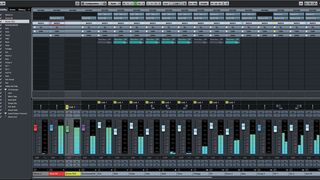
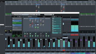
• Creating a well organized mix session in our DAW that assures we can apply our sonic ideas quickly
• Building a strong foundation for our mix by balancing the low end, and saveguard our creativity by always retaining plenty of headroom • giving special attention to the lead vocals, assure they have a round tone, cut through the mix, and have plenty of attitude
• Creating continuity throughout the mix • using parallel compression to add weight and impact on our most important elements in the mix
We now have a very solid foundation, but the mix still sounds one dimensional and static at this point - which is what we’re working on in this chapter to finalize our mix!
EQ-ing
Here’s something you need to get your head around. We’re mixing MUSIC. Try to see the following in every element of your mix:
• Fundamental note/tone
• Harmonics on top of that (often in form of a triad)
• A noise component added to that, mainly in the high frequencies.
The frequencies in your mix should form a smooth texture where the different instruments add up to a rich spectrum of colours. Don’t take this too literally, but think in musical terms when EQing, and keep that in mind while we go through the tools available to create this. Boost frequencies that build a triad, spread wider in the low register, and you can go more narrow in the higher mids. EQ-ing treble is a matter of asking if you want highs on this instrument or not? If yes, how much until they hurt your ears?“ The chart below can help, but always keep in mind, don’t take this too literal. PIANO KEYS TO FREQUENCY CHART Before we have a look at the important types of EQs, and where to use them, know that you will need to use a combination of these to cover all your EQ-needs in a mix. If you are not yet familiar with those classifications, take some time to explore the possibilities of these on different sources. In the context of setting final levels in the mix, which we get to at the end of this chapter, EQs can be used in a very basic way. When you level for example a piano or guitar in the mix, this is as simple as having the upper range of the instruments, including the noise component (piano hammer noises, guitar picking noises) sit right in the mix first, and then use a broad EQ between 200 - 400Hz to adjust the lower range of the instrument by boosting or cutting.
Classic EQ-types

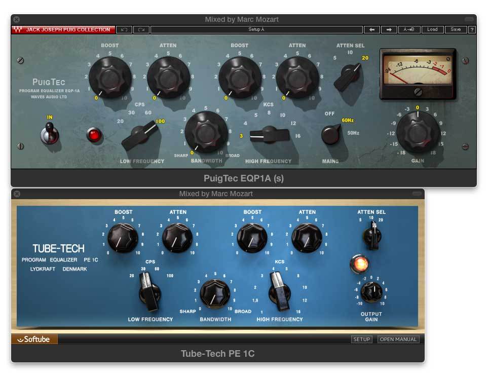
„Pultec“-type EQs
Probably the EQs I personally use the most in my mixes - the hardware-versions of these are tube-compressors that come in two basic types: 1. the EQP-1 „Program Equalizer“ can boost and reduce bass at the same time (in steps from 20 to 100Hz), and has similar controls plus a bandwidth-parameter for treble (switchable boost for 3, 4, 5, 8, 10, 12, 16kHz, Attenuation/Reduction for 5, 10, 20kHz).
The MEQ-1 „Midrange Equalizer“ is an EQ for mids - it has a boost (here called „Peak“) for selectable lower mids (200, 300, 500, 700, 1000Hz), a selectable „DIP“ (reduction) for 200, 300, 500, 700Hz, 1, 1.5, 2, 3, 4, 5, 7kHz and another boost for high mids (switchable between 1.5, 2, 3, 4, 5kHz).

Pultec-type EQs are great for shaping tones in a very natural way. It is difficult to get a bad-sounding result out of them. Even when frequencies are fully boosted, the boost still has a smooth and natural character about it. The reason for this are the Pultecs broad EQ curves. Even when you boost below 100Hz, the boost reaches up to 700Hz. While these EQs have their own character, you can learn from them even if you don’t own one. Simply try out broader curves (smaller Q-factors) with the EQ you have at hand. The EQ-part of the Pultec consists of „passive“ electronics that reduces gain internally, and the tubes are used for a 2 stage line amplifier to make up for the gain lost in the passive EQ-circuit. There are a couple known variations of these from known manufacturers, and an almost endless number of plug-in versions. While the original hardware-versions are amongst the most expensive EQs you can buy for money, plug-ins are of course a way to use these on pretty much every source in your mix. Note that Pultecs add a very desirable and subtle tube saturation to your signal even when the EQ is set flat.
PULTEC EQs – APPLICATION EXAMPLES
Pultec MEQ 5 – WARMTH ON A VOCAL
The Pultec MEQ 5 is usually my first EQ in the vocal chain, using a broad boost between 200 – 500 Hz, but you can simulate these (broad) curves with many stock EQs that come with your DAW. I don’t ever go lower than 200 Hz, and occasionally up to 700Hz. The effect we want to get here is that the vocal gets more weight and warmth in the mix. If the vocal is well tracked, it comes with a lot of that quality in the recording and you may not need to do anything here. This is why people use Neve 1073s and various tube-based equipment (from Tube Mics, Tube Mic-Pres to Tube Compressors) during tracking. However, a lot of modern vocal recordings sound rather thin, and a nice boost in the low mids can fix that. If you like the character you’re adding with the boost, you can even do a little bit too much of it. You can counterbalance it later in the chain, for example by using a gentle compressor like a Fairchild or Summit TLA-100A. In case the vocal already sounds overly „muddy“ or „boomy“, add a Linear Phase EQ at the beginning of the plug-in chain, locate and remove the frequencies that cause this effect. Watch the interdependence of that – once you’ve removed resonances, you have more leeway again to use that broad Pultec-boost again.
Pultec EQP-1a – FINAL EQ ON A VOCAL CHAIN
A Pultec EQP-1a as a final EQ can round off treble and bass. I like a Pultec EQP-1a here, to boost at 20Hz, and Attenuate at 20kHz. Your vocals will sound more analogue when you roll off the top end – I always do that at least slightly, sometimes a lot. Both the boost at 20Hz, and the attenuation at 20kHz should not affect the essence of the tone you have created. The boosts can add little bit of weight, and the cut removes top end energy that only hurts at loud volumes.
Pultec MEQ 5 – WARMTH ON THE STEREO BUS
Similar to the vocal chain, the MEQ 5 is boosting when „warmth“ is needed. Test if our mix bus lacks anything between 200Hz and 700Hz by switching through the frequencies. Don’t boost anything just because you can. Try the same with the upper band as well – a little boost between 1.5k and 7k can add some energy. On all accounts, I’m talking about a +2 or +3dB boost here at best – which is still a very subtle amount on the Pultec.
Pultec EQP-1a – FINAL TONE CONTROL ON THE STEREO BUS
Again the Pultec EQP-1a (never confuse it with the MEQ used above) does a subtle boost here, usually 2dB at 20Hz, and I attenuate treble by 2dB at 20kHz. Another very „esoteric“ setting, the Pultecs on my mix bus are mainly used to add an analogue vibe.
Classic console EQs (SSL, Neve, API)

These are the EQs found on the most popular large format recording consoles from the 1970s until today. You don’t need to own a recording console as all of these are available as hardware from the original manufacturers, for example in the popular 500-series format. Console EQs were designed to be able to shape all kinds of signals. They usually have a shelf EQ for the lows and highs, and 1 or 2 bands or fully parametric EQs for the mids. These can often reach as high or low as the low and high shelf EQs. Today, most people learn about and use them in the form of plug-ins, some of them developed with SSL, Neve or API. I might be a bit simplifying here - but you mainly use these when you want to boost or shape a sound more narrow, or more agressively than what can be achieved with the Pultec-type EQs.
CLASSIC CONSOLE EQs – APPLICATION EXAMPLES
SSL EQ FOR PRESENCE IN A LEAD VOCAL
In a dense mix, we need to create frequencies that make the vocal cut through the rest of the instruments. We can go to extremes here, but before you start playing with the mid boost, set up a compressor that follows it right away. It’s needed to tame the mid boosts as they can get very harsh. Often, less or no boosting in the mids is needed in less populated parts of the song, but when the vocals are up against a wall of sound, you will need a musically composed texture of „cut through“ frequencies there. This is more complicated to get right, compared to creating warmth. Start with an SSL-type EQ and boost the high shelf at 8k +10dB, then pull back again to 0dB and find a great setting for it somewhere in the middle. Try switching between BELL and SHELF characteristics (BELL will just boost around the set frequency, while shelf also includes all frequencies above. If 8k is boosting sibilance too much, go a tiny bit lower. Continue by using the HMF band to boost at 4k. And the LMF to boost 2k. Move these around until you find a good balance – but keep in mind, not boosting anything is always an option. The goal is to create a cluster of mid-boosts that appears as one colourful and musical texture of mid-boosts between 1 and 8k. Chris Lord-Alge is a master of this technique, and you can learn a lot from him by studying the Chris Lord-Alge presets for the Waves SSL Channel. Check specifically the “Rock Vocals” preset. You will probably be able to achieve good results with the stock EQs of your DAW, but there is a reason why SSL EQs are famous for their musicality in the mids. API, Neve works as well. Not a job for a Pultec.
Linear Phase EQs
These are digital EQs, and they were first introduced as super expensive digital outboard boxes for mastering engineers, who have used them for many years. Like everything expensive and digital, it is now available in plug-in form, and for example Logic Pro has a very good linear phase EQ that comes with the software. There is a ton of technical info on linear phase EQs on the web, none of which will help you improve your mix. One thing they all have in common is adding a significant latency to your signal that needs to be compensated for by your DAW. This is a problem when using it on live instruments, but not in mixing. As shown in the chapter on parallel compression, just make sure your plugin delay compensation is switched on across all types of audio tracks, and you’ll be fine using linear phase EQs. The reason for the added latency is that instead of „post ringing“ which we see in traditional EQs, the linear phase EQs adds „pre ringing“, which in turn keeps the phase response linear. All you need to know is that the linear phase behaviour makes these sound more neutral and less drastic. They don’t add harmonics and resonances - their effect is totally isolated to the frequency range you have selected. They can be used for boosting and attenuating, both broad and narrow.

LINEAR PHASE EQs – APPLICATION EXAMPLES LINEAR PHASE EQs – USING NOTCH-FILTERS TO SURGICAL REMOVE “STUFF” & BOOSTING SPECIFIC FREQUENCIES WITHOUT AFFECTING ANYTHING ELSE
Linear Phase EQs are unbeaten to do “surgical” operations on your audio material. If you need to remove a specific frequency, for example a room resonance in a live recording, you can set a very high Q-factor and create a notch filter at this frequency that will not affect anything else. All other EQs listed here operate much broader, even when set to a high Q (note: high Q-factor = narrow EQ = notch filter; low Q-factor = broader EQ-curves). This can also be useful so discretely boost specific frequencies. Very useful when targeting the exact fundamental root note or 1st harmonic on a kick drum. Again, set a very high Q, and a linear phase EQ will boost just that narrow band. Analogue EQs are known to create harmonics above the boosted frequency, and will also start to self-resonate at high gain. Which is what we sometimes want – but not always.
LINEAR PHASE EQs – FINAL TONE CONTROL ON THE MIX BUS
I also use a linear phase EQ as my final control for the overall frequency curve of the mix. I usually add a very broad and subtle boost on the bass, add or remove mids broadly by a maximum of +- 1dB, and check if there’s room for a bit more “sparkle” around 12k. Again, I’ve made all musical EQing before that so I want an EQ here that does not create any harmonics. After all, it’s the final stage of my stereo bus.
Filters
To list filters here is somehow redundant. Filters always come in the package of most EQs, except the Pultec-type. You use them to remove frequencies below a certain frequency (HPF = High Pass Filter = high frequencies are „allowed“ to pass) or above (LPF = Low Pass Filter = low frequencies are passing). The most popular application is a HPF on vocals, to remove low "rumbling", commonly frequencies below 60 - 120 Hz.
FILTERS – APPLICATION EXAMPLES
FILTERS – REMOVING LOW-END RUMBLE ON A VOCAL RECORDING
This is of course a widely known technique – many people use a high pass filter (HPF) set at around 70Hz in their vocal tracking-chain, to remove low-end rumble that is caused by the environment, but doesn’t contain any frequencies from the recorded source.
FILTERS – FOCUSSING A SOUND
You can use a combination of HPF and LPF to focus any sound to a specific frequency range. Sounds tend to “sit” better in the mix when you limit their range. Just as an example, try reducing anything above 10k on a synth-bass. When solo’d it might sound like you take something away from the sound, but in the context of an entire mix there are other instruments that need that space above 10k. Same goes for guitars, pianos, synth-stabs, etc. – by limiting the frequency range an instrument is easier to identify in the mix which in turn contributes to the overall three-dimensionality of your mix. On many, if not most of my DAW-channels, I’m using ALL of these EQs at different stages of the plug-in chain.
A different look at compressors
We all have a basic idea of what a compressor does and how to use it, right? I’ve googled „what does a compressor do?“ and the „top“-results are pretty much all similar but still wrong. Something along these lines: „Compression controls the dynamics of a sound, it raises low volumes, and lowers high volumes“ This sub-chapter is about compressors as a tool to shape the tone of a signal via adding harmonics. There might still some level correction involved, but as pointed out in Chapter 7, correcting drops or peaks of level at the source is preferable to using a compressor for that. Personally, I think of different models of compressors in terms of „how they feel“. The choice becomes intuitive, as a compressor imparts a distinct characteristic on a sound, pushes it into a sonic direction. It took me years of practise to develop that feel for certain types of gear. It’s more difficult to develop when you use only plug-ins, but you can still get to similar results with both hardware and plug-ins. The original hardware counterparts are different in that they show a lot more color and distortion when you drive them to extremes. Those extremes helped me to learn the characteristics. Since that won’t help you - unless you have access to a studio with a large analogue outboard collection - this post is taking an analytic look into popular compressor plug-ins and their characteristics.
TEST SETUP & PROCEDURE
Let’s run some popular compressor plug-ins through a test setup and procedure, then look at what the results tell us!
The Test Oscillator in Logic Pro X feeds a compressor with a test-tone
• the test tone is a sine-wave (as you know, a sine-wave has no added harmonics). • we cycle through 55 Hz, 110 Hz, 220 Hz, 440 Hz tones • then a sweep from 20 Hz to 20.000 Hz • ending the cycle with a 100 Hz tone
we cycle through this 3 times, with rising levels 1st Cycle
• Oscillator hits Compressor with - 18 dB of level • Compressor Threshold is set JUST BEFORE compression • for the compressor NOT to compress (unity gain)
2nd Cycle
• Oscillator hits Compressor with - 12dB of level (6 dB more than on the previous cycle) • Compressor settings stay the same, but of course compression now kicks in!!
3rd Cycle
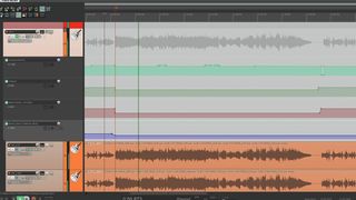
• Oscillator hits Compressor with – 2 dB of level (another 10dB added on top of the previous cycle) • Compressors settings remain the same, but now hitting compression quite hard! The upper track you can see in the videos is the automation curve for the Test Oscillator’s frequencies and levels, the lower track shows a huge analyzer plug-in after the output of the compressor (using Logic Pro X’s Channel EQ), and that shows as the frequency spectrum in realtime. BTW: – 18 dB in your software is a GREAT average level for your recordings and signals in ALL situations. It assures clean and pristine sound and compatibility with all plug-ins.
Summary: on the first cycle, the compressor doesn’t actually change the level of the signal, on the 2nd cycle there is some compression, and on the 3rd cycle: a lot.
Every cycle ends with a 100 Hz tone – that makes it easy to read the added harmonics on the analyzer. 2nd harmonic = 200 Hz 3rd harmonic = 300 Hz 4th harmonic = 400 Hz 5th harmonic = 500 Hz n th harmonic = 100 Hz x n Just for reference, here’s what the test procedure looks like with NO COMPRESSOR inserted in the signal path.
As you can see, the analyzer just shows basic sine-tones, with no added harmonics. Music theory and physics calls this is the 1st “harmonic” – but don’t be confused, that is the term for the original frequency of the sine-tone.
FAIRCHILD 670 COMPRESSOR (1959) – THE ROYAL HARMONICS ORCHESTRA
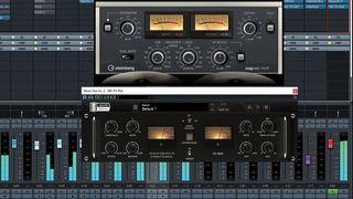
To give you a proper contrast – here’s what this looks like with a plug-in clone of the legendary Fairchild 670 compressor, as some of you might know, the most expensive and sought after vintage tube compressor on the market.
I bet you that the designers of this plug-in looked at a spectrum like that forever, and did endless coding and testing until the plug-in matched the original hardware closely. You can already see some harmonics even when the compressor doesn’t compress, but they really kick in the more you compress. Note: the lower the sine-tone, the more harmonics show up – I can count 13 added harmonics in the 3rd cycle on top of the 50 Hz sine tone. When the oscillator reaches 2000 Hz, the Fairchild doesn’t add more harmonics on top, at least not visible anymore in the spectrum. If you look at the rich harmonics added by the Fairchild, you start understanding how it gives a dull bass-sound or a 808 subsonic kick a richer frequency spectrum. This is very useful as it helps low-end to subsonic sounds to translate better on smaller systems (think laptop, tablet, smartphone, kitchen radio). At the same time, a Fairchild might not be the ideal compressor to purely control volume, because the more you compress, the more it changes the sound of the source. This is not typically what you need if your goal is to level something that is dynamically uneven. On the contrary, you want to make sure that your source is already in control dynamically BEFORE you even hit the Fairchild. There are other ways to achieve a consistent loudness in a performance. Look at waveforms of your recording and just bring the lower parts up in level, reduce loud sections, automate, and a lot of times, a consistent level is what a great performer brings to the table! If your signal is well-levelled and even, you can alter its tone by the amount of drive the signal into compression. I’m almost ready to go into detail on parallel compression at this point – imagine a setup where you’re bring the same low 808 Kick into two mixer channels. The first channel kept unprocessed, the second channel pushed hard into a tube compressor like the Fairchild – the added tube channel will make the 808 come through on smaller systems and adds a nice texture to a sound thats pretty close to a sine-tone. On the parallel channel you can even cut off the low end and just add the harmonics (of course cut off POST compression) – more about that in Part 2 of this article. Essentially, what the added harmonics do is adding frequencies to the original sound that weren’t there before.
PUT THE COMPRESSOR IN THE MIDDLE OF THE SIGNAL-CHAIN
A typical signal chain around a compressor like the Fairchild would look like this:
Source Signal
-> Surgical EQ (to remove unwanted frequencies) -> Compressor (adding harmonics) -> EQ (for color and tonal balance)
PRE COMPRESSION:
Surgical EQ removes unwanted frequencies It’s very important to put an EQ BEFORE the compressor. Use this EQ to remove unwanted frequencies. Typical example would be a High Pass Filter that removes rumbling impact noise on vocal recordings. Imagine how the Compressor would add harmonics to a rumbling noise at 30 Hz and really bring it out – you don’t want that. Same goes for unpleasant room resonances – find them using a narrow EQ boost then set a small notch to remove them. This so-called „surgical EQing“ works best with „Linear Phase EQs“ – many plug-in manufacturers make them, they don’t add coloring resonances. I like the one that comes with Logic Pro X a lot.
POST COMPRESSION:
EQ for color and tonal balance Going back to the example of a low 808 subkick, which is a sound that is very similar to the sine-tone used in our test, there would be no point in EQing a pure sine-tone, right? You can’t add frequencies that are not there – in contrast to a tube compressor, an EQ does NOT generate any frequencies, it can only adjust the tonal balance of the given frequency-content. With that, we have once again turned common audio-knowledge upside down: Compressors can add color to any frequency EQs are static, all they do is adjust the tonal volume That rule is of course not totally holding its own once we look at a few more types of compressors. What we’re interpreting in this article focusses on frequencies and harmonics, which is just one aspect of compressors. The other one is the actual ability of a compressor to level, limit or „grab“ a signal, attributes that all refer to the volume of the sound.
UNIVERSAL AUDIO/UREI LA-3A (1969)
The Waves CLA-3A is a plug-in clone of the original Universal Audio LA-3A Compressor/Limiter. In contrast to the Fairchild, it’s a lot better suited for levelling a signal. The LA-3A adds only one harmonic (the 3rd one). The Fairchild and the LA-3A can co-exist in a signal chain. Use the LA-3A to even out levels, then hit the Fairchild. The LA-3A is typically used as leveller for bass, guitars and even vocals. Less suitable for percussive sounds – it’s not following fast enough to control a drum sound.
TELETRONIX LA-2A (1965)
The Waves CLA-2A is a clone of the Teletronix LA-2A. The design is a few years older than that of the LA-3A. It adds more harmonics than the LA-3A, but still a lot less than the Fairchild. Typically used to control bass, backing vocals or laid-back lead vocals. A fairly slow and laid-back tube compressor.
UNIVERSAL AUDIO 1176 REV. A BLUE STRIPE (1967)
The Waves CLA-76 is a clone of the Universal Audio/UREI 1176. Various revisions were made, the „blue stripe“-version being the first one ever created. Nearly every plug-in manufacturer offers a clone of the 1176. I like the ones made by Waves, and they got their name because Waves developed them with Mr. CLA aka Chris Lord-Alge. The 1176 displays extremely rich harmonics. In comparison to the Fairchild 670, it sounds a lot more agressive and levels superfast. That makes the 1176 very flexible – it can be used on almost any source. Like the Fairchild, the 1176 is a true studio classic and it would be worth writing a dedicated chapter about it. If you have a bunch of those in your rack (or a great plug-in clone in your collection), you could mix an entire project exclusively with those. One of the things it works very well for is making vocals agressive and bring them upfront. You can drive it hard into a lot of compression, and as a result will see a lot of harmonics. It would not be the only compressor in the chain, I’m usually running another compressor for levelling before the 1176.
SOLID STATE LOGIC SSL E/G-SERIES BUS COMPRESSOR (1977)
This is of course one of the most famous compressors ever build. Waves teamed up with SSL to create one of the first true emulations of an original hardware, and this plug-in (as part of the Waves SSL-bundle) is now a classic, just like the original SSL 4000E and G-Series consoles. It does – of course – a great job levelling a signal, and adds more harmonics the harder you hit it. The trick with the SSL Bus Compressor is hit compression with your peaks in your finished mix, e.g. the kick drum. What happens is that the SSL „grabs“ and reduces the peaks in a very clever way, while adding harmonics to them. The SSL bus compressor controls the dynamics and makes the bits it compresses more punchy by enriching it with harmonics (almost like compensating for the lost level). This effect has widely been described as mixbus-“glue” and the reason why everybody loves SSL Bus Compressors.
SOLID STATE LOGIC SSL E-SERIES CHANNEL COMPRESSOR (1977)
The SSL Channel Compressor, also a part of the Waves SSL-bundle, adds a healthy portion of bright and agressive harmonics, and is capable of controlling and “grabbing” percussive signals like no other compressor. Widely used by famous mix engineers on Kick, Snare and any type of percussion – the SSL gives drum sounds a prominent place in the mix, makes drums punchy and cut through.
SUMMIT AUDIO TLA-100A (1984)
The Summit TLA-100A is a very subtle tube compressor. The original analogue hardware has been used by engineer Al Schmidt as a tracking compressor on many of his Grammy-winning projects, for example on Diana Krall’s vocals, to catch some peaks with light compression during vocal recording. The Summit adds some harmonics when you drive it, and works well on a wide selection of sources with 3 easy settings for both attack and release-time. A very subtle leveler for tracking and mixing.
LOGIC PRO X COMPRESSOR (PLATINUM MODE, 1996)
This is the original compressor plug-in that came with the first version of Logic, so the design goes back to the mid-90s. It’s actually the ONLY plug-in in our test that does not colour the signal AT ALL. Contrary to all other compressors tested, this is a compressor suitable for applications where you want to iron out the dynamics of a track without adding harmonics. The later versions of this plug-ins (like the current one in Logic Pro X) added a few more modes you can select, and when you switch from the “Platinum Mode” in any of the others (like “VCA”), the plug-in starts adding harmonics, trying to mimic some of the compressors I just introduced.
u-he PRESSWERK (2015)
If you don’t have a huge collection of outboard and/or plug-in compressors, you can start with just one that delivers a broad range of application. I personally very much like u-he PRESSWERK which is currently the only compressor plug-in on the market, where the amount, dynamics and shape of the added harmonics can be set independently from the amount of compression. If you look at the block diagram, you will see that PRESSWERK unites all the features and topologies found in classic 1950 – 1970 compressors, while giving the user full control over these features and clear labels to access these in detail.  I can see PRESSWERK becoming popular in audio schools, as there’s no other plug-in that will make it that easy to educate someone about the details of ALL vintage compressors in one plug-in. All of the emulations I’ve tested earlier in this chapter, except one, generated harmonic distortion, and these would usually increase in level the more gain reduction (= compression) you’re applying. With PRESSWERK, you have total control over the amount of harmonics that are added, and the DYNAMICS-control can seamlessly adjust between „depending on the volume of the source material“, and „harmonics always added“.
I can see PRESSWERK becoming popular in audio schools, as there’s no other plug-in that will make it that easy to educate someone about the details of ALL vintage compressors in one plug-in. All of the emulations I’ve tested earlier in this chapter, except one, generated harmonic distortion, and these would usually increase in level the more gain reduction (= compression) you’re applying. With PRESSWERK, you have total control over the amount of harmonics that are added, and the DYNAMICS-control can seamlessly adjust between „depending on the volume of the source material“, and „harmonics always added“.
The basic harmonics added look somewhat similar to these of a classic UREI 1176 blue stripe, but the various controls of PRESSWERK’s saturation section can highly customize them, for example apply them either PRE or POST compression, statically or following the dynamics of the material, and you can also balance the spectrum of the harmonics slightly using the COLOR-control which is essentially a „tilt“-type filter/EQ. When you watch the clip, pay attention at me playing with the Saturation-section of PRESSWERK starting at around 1:11min.
You can download a demo of PRESSWERK HERE: Saturation is of course something that occurs - more or less - in all analogue signal processors, not only compressors. It’s worth mentioning a few more „stand-alone“ boxes/plug-ins that can be used to generate harmonics via saturation.
Tape Saturation
Reel to reel analogue tape machines - remember those? A magnetic recording „head“ magnetizes a magnetic tape that can run at different speeds. Analogue tape, when pushed with extreme levels, doesn’t distort the same way as a digital converter does. The more you enter the „red zone“ of a tape machine, you get an effect called „tape saturation“. The sound of tape saturation varies of course with the type of tape recorder, width of tape, and tape speed. The classic analogue studio standards by STUDER or AMPEX are still loved for their sound, but are rarely ever used these days. Plug-in emulations have come a long way and do a really good job getting this type of sound in your DAW.
Mic Pres
Microphone Amplifiers or short „mic pre’s“ come in flavours similar to compressors (minus the gain reduction circuit) - they can be build with tubes, transformers, transistors or modern OP-amps, or a mixture of all of these technologies. Some of them can also be used at line-levels, and also make a great colour in your palette - especially if you do vocal recording as well. The various Neve-models come to mind, they are amongst the most legendary studio classics. While the original versions are extremely costly, both AMS Neve and various other companies build stripped-down alternatives such as 500-series modules. The classic Neve 1073 is also widely been modelled as a plug-in.
Magic Chains
As you expand your knowledge about processing and plug-in chains, I recommend that whenever you have found a combination of settings that works in a mix, save the entire channel strip as a plug-in chain in your DAW. Make sure the name you’re using reminds you about what the application for this preset could be. Over time you will develope a library you can always go back to and further refine.
Reverbs and Delays
Most producers have a very basic set of Reverb Sends and Returns in their DAW sessions: a standard reverb (mostly plate or concert hall), one delay for throws, and maybe a small room simulation with early reflections. All the tracks in the arrangement are accessing the same reverb and delay, if needed. Thats totally fine for arranging and producing, but forget that concept for your mixing-session. If you want to create an impression of a 3-dimensional mix, with lots of space and separation, here are some things you need to think about: you need a huge palette of different reverbs and delays, add to that some modulation FX the reverb you end up with will be a mixture of several reverbs that differ in many ways, from colour and density to reverb time the most important tracks in your mix are accessing completely different reverb and delay sends and returns you need to have banks of different reverbs ready in your DAW template, specialized for different sources like drum room, snare, toms, lead vocals, pads, lead synth, orchestral instrument group the reverb returns together with the instruments they belong to - if you have a drum subgroup or VCA group, the reverb returns for the drums belong to that, and exclusively to that also, you don’t need to create a new send for every reverb - you can send, for example, to 20 different snare reverbs from „Send 5“, and then just unmute and mute them at the aux return, one at a time, until you find what you’re after; this is a very fast and intuitive process, and gives you the option to use one or several reverbs at the same time, and level their balance at the different reverb returns for subgroups or VCA groups to really work, FX belong mostly exclusively to their sources - if you mute the drum group, you mute all drum reverbs with it, but of course NOT the vocal reverb it’s essential to stay very organized in that respect All of the above probably sounds my mixes are drowning in reverb. Don't be fooled - some of these are very subtle. Also, don't be afraid of long reverb times, but keep them super low in level. Many of these you only hear when you switch them off. Here are some examples for types of reverbs that are useful to have at hand, all at the same time: most reverbs deliver sounds in categories like plate, chamber, ambience, rooms, concert halls, church, etc. most classic reverbs (e.g. Lexicon 224, 480, EMT, AMS RMX) are great at less defined, „cloudy“ reverbs, regardless at which reverb time modern reverb plug-ins and hardware reverbs (Bricasti M7 is my favourite) are great at super-realistic room simulation plug-ins using IRs (Impulse Response) can do both - IRs are basically just samples or „fingerprints“ of the original reverbs or even real rooms What I personally have done over the years was simply try a lot of different reverbs and especially IRs, and every time I heard something that I liked, I saved the channel strip settings, reverb, EQ and some compression, to a channel strip preset in Logic. Doing this will allow you to keep developing a go-to library, and certain reverb chains you can not live without after a while, and these make it to your DAW mix template. Delays also come in many different flavours: the typical 1/2, 1/4 or 1/8-note delay „throw“, often used on the last word or syllable of a vocal-line. short slap-back delay complex delays with polyrhythmic patterns, or even unpredicted „weird“ stuff happening in the feedback loop Reverbs and delays are to your mix, what a shadow is in a photography, you don’t want them as sharp and shiney as your main object. Most of my delay returns are sending to reverbs as I don’t like them to be a totally dry „sampled“ copy of my original signal. Look at reverbs (and delays) similar to a shadow in a photography, you don't need them 100% upfront, shiny and dynamic, their purpose is to give you a sense of subliminal depth. Compressing them helps that a lot. I also EQ them contrasting to the direct signal for that reason, so if you've worked hard to make your lead vocal upfront, direct and "in your face", you don't want to send your reverb from that direct signal. BTW, this is one reason why older "vintage" reverbs/delays are still popular - they have a low-res, "grainy" feel about them (example Lexicon 224 or AMS DMX1580). Compressing reverbs also makes them more controllable - you can get away with less reverb in the mix, if you compress the reverbs that you are using.
Creating a three-dimensional sound
There are obviously a lot of small details involved, but for a start, get your head around the following concept: important stuff goes to the center: Kick, Bass, Lead Vocals try panning everything else hard left or right Sounds crazy I know. Try panning a guitar hard left, send it to a small room and pan the room hard right. Now bring the reverb a tiny bit more to the center until it feels well-balanced. The second guitar you might have: pan the dry one hard right, send it to another small room (or delay or chorus) and pan the effect hard left. You get the idea… this works for guitars, keyboards, percussions, noise fx, etc. - I use small rooms/chambers/spaces from the Bricasti M7 reverb for that. There are Impulse Responses for the Bricasti out there - for free, and officially authorized by the guys who designed that reverb.
Modulation FX
re: rhythmic gating, the Tremolo (modulates only volume) in Logic Pro is a secret weapon.

I use this all the time on lifeless or over-compressed tracks - brings some subtle movement into them. From pads to static synth basses to heavy guitar chords to backing vocals. You can even make reverbs groove subtly with the beat.

Subgroups, FX Busses and Routing
As the number of different reverbs (delays, etc.) you are using grows, you need to keep the routing strictly organized. Using the same reverb on several sources quickly becomes messy. You might need to EQ or compress your main reverb in a certain way to improve its sound on the vocals, but as you have used that same reverb on other instruments you are suddenly affecting the balance and sound of your entire mix. I know it sounds counter-intuitive, but you’re better off separating the reverbs you are using for the different instrument groups, which includes the routing and grouping. On my console, I have a pair of channels dedicated to vocal reverbs, another pair for drum reverbs, and they are assigned to their respective VCA groups. On the drums use pre-fader sends, use the drum fx exclusively for drums, and route their returns to the drum bus as well, and/or put them on the same VCA group. Same goes for parallel compression busses, the sends to them are pre-fader, not following automation, but the returns follow the automation of the source - I do that via the Drum VCA group - you get the added bonus that you can treat the FX returns for each group of instruments separately. We want total control in mixing.
Stereo Bus Magic?
A very popular question… „What’s on your mix bus? Are you using PRODUCT X or PRODUCT Z like I do?“ „All in one“ mix bus processors promised to be the one stop solution since the first TC Finalizer that came out in the 90s. You all know the various modern plug-in equivalents of that, and to a certain degree, they work really well. A quick preset can make a song demo more presentable. Things that are involved in these processors are multiband-compression, stereo processors for more width, psychoacoustic loudness treatment, and of course EQs, compressors, limiters, etc. The disappointing truth is that you really need to make your mix happen before the signals gets to the stereo bus. If the mix is rotten at the core - and I refer you to all the things we’ve looked into from the Chapters 3 to this point, multi-band compression can create more density and loudness, but never solve problems that were ignored in the first place. With that, let’s go through my common mix bus signal chain, and allow me to add that every single processor used here is doing only extremely subtle things.
1. Loudness Meter
From the very start, embedded in my template, the first plug-in on my mix bus is a loudness meter - it monitors the level of the signal that comes in. We talked about Gain Staging in Chapter 5, so you know what to look for. Also, at this point let me remind you about best A/Bing practise as discussed in Chapter 3: we can A/B between a treated and untreated version of our mix bus, at matched levels. This is essential when working with plug-ins on the mix bus - you might not need ANYTHING here.
2. blank
I’m not joking. It’s a blank plug-in slot with no plug-in inserted. Leave it like that because if anything comes up, you can insert whatever you might need later on.
3. Midrange
The combination of plug-ins I use here is EXACTLY the same that I’m using on vocal-chains:
A. Pultec MEQ 5
Remember, this was where on the vocal chain, a Pultec is boosting when „warmth“ is needed. Test if our mix bus lacks anything between 200Hz and 700Hz by switching through the frequencies. Don’t boost anything just because you can. Try the same with the upper band as well - sometimes a subtle boost between 1.5k and 7k adds some energy. On all accounts, I’m talking about a +2 or +3dB boost here at best - which is still a very subtle amount on the Pultec.
B. Tube compressor for tone
I use a plug-in version of the classic Fairchild here, and settings could be called „esoteric“. The gain reduction-needle is hardly ever moving, but when I A/B, it ALWAYS sounds better with the Fairchild in the chain. The category here is mid-range, as it adds harmonics.
4. Final Tone and Dynamics Control
A. EQ
Again the Pultec EQP-1a (don’t confuse it with the MEQ used in step 3!) does a subtle boost here, usually 2dB at 20Hz, and I attenuate treble by 2dB at 20kHz. Another very „esoteric“ setting, the Pultecs on my mix bus are mainly used to add an analogue vibe.
B. Final Dynamics
I happen to use Slate FG-X as a final bus compressor, and also use the Transient, ITP and Dynamic Perception Controls to fine tune. I am NOT using FG-X as a brickwall limiter, and my signal is leaving this plug-in with the same amount of headroom left as it’s entering it. The „constant gain monitoring“-button is always pressed for that reason.
C. Linear Phase EQ
This is my final control for the overall frequency curve of the mix. I usually add a very broad and subtle boost on the bass. And one more time: keep going back between these building blocks for fine tuning. Watch the gain staging!
Automation
Let’s go back to a concept that was introduced in chapter 7 - correcting and automating levels PRE and POST plug-in chain. PRE is to create a consistent natural sounding performance, which we already dealt with. The automation we are now working on is the POST plug-in chain automation that creates your dynamic for the song. Of course, even once you start activating the fader automation in your DAW, there will be situations where you need to change the entire relative volume of the track. A simple gain plug-in before the automation fader gives you easy access to the relative level of the entire track - which is a lot easier than always correcting the entire automation. The way this is handled differs slightly between DAWs, and console automation might have other ways to deal with relative levels. Make sure though to find out how to independently deal with relative levels and automation, both POST plug-in chain of course. Another issue we have already dealt with in Chapter 7, but I’ll repeat it here again - if one instrument has completely different levels or settings in different songparts, instead of creating automation for that, just copy the channel settings and have an extra channel for different song-parts. And… another reference to an earlier chapter: automation is best performed or programmed while listening at low levels on your small portable speaker. Automation is a great place to emphasize the natural dynamics of the song. Let’s face it - on a rock-song, the drummer will hit the drums harder on the last chorus. Keep in mind that this is not totally depending on levels, as more intense drumming will reflect in brighter drum tones. But still, a subtle push in volume on the final chorus can create extra excitement. This is where the final balance and automation of the mix can be compared to car racing, and you will face the same dilemma as the race car driver: you want to drive as fast and risky as possible, without destroying the car. Luckily, with a few safety features in place, automating a mix is still a very enjoyable ride (and much less dangerous compared to car racing). These are the safety features: • if you have „nulled“ your faders, like described in Chapter 7, and maintained solid gain staging throughout adding treatment of the individual channels, you have a „unity gain“ default position for your faders, which means there is zero chance to destroying the solid balance you have already created up to this point - you can always go back to start. When you work your automation around the 0dB position of your fader, you have a much broader range to do subtle fader movements. 3dB is still a bit of movement around the 0dB-point - try to perform a 3dB increase when your level sits at -30dB default! Impossible. That goes for both physical faders and visual automation data in your DAW • oh yeah, you have of course saved your project under a new version number on a regular base - so that you can always go back in case your mix gets worse • the stereo bus treatment we’ve setup in this chapter will make sure that your dynamics stay within a certain range. If your bus-compressor has the right setting, it will subtly keep your dynamics within the frame of good gain staging - in other words, if you push signals into the stereo bus with more level, the increased level at the channels will partly be compensated for by the ratio set on the bus compressor. • and one more last time: your portable speakers at low levels will assure that you’re staying in the right frame with your automation With that - go and create excitement in your automation! Go for bold moves! Definitely start learning to automate with faders. Drawing automation with a mouse will never replace your hand on a fader while closing your eyes and listening to the song at low volume. As a final note on automation, know that you will also have to go back and forth between setting levels and EQing. Whenever there is a situation where you feel the track sits great in the mix, but the bottom is to thick or thin, you know where to find the handle for that. The levels of the track are right when you can even hear very subtle level-changes. As long as you can still move the levels of an instrument up and down a few dB, and it makes no difference for the mix, you need to go back to the start of this chapter and use tools other than level to make the signal sit right in the mix.
Reverb Culture - using Reverbs and Delays in the mix.
Most producers have a basic set of Reverb/Delay Sends and Returns in their DAW sessions: a standard reverb (mostly on a 3 sec plate or concert hall setting), a delay for throws (with feedback for repeating echoes), and maybe a small room simulation with early reflections. All the tracks in the arrangement are accessing the same reverb and delay, if needed. Thats totally fine for arranging and producing, but forget that concept for most mixing-sessions. I’ve called this sub-chapter “Reverb Culture” as there is a million things to explore when it comes to reverbs and delays. The more you explore the subtleties of different types and colours of reverbs, you want to start using them in your mix. You can use reverb to improve the “front - back” dimension in your mix, placing certain instruments more distinct on a virtual stage, creating contrast between the upfront/direct and the more unobtrusive elements in the mix, and much more - reverbs offer a microcosm of endless possibilities.
A little bit of reverb history
Hundreds of years ago, classical composers thought about how to set up the musicians on stage, and the traditional setup of an orchestra is arranged in a way that certain instruments have more room ambience added as they are further in the back. A good example would be brass and timpani, which are seated at the back of the orchestra, behind woodwind and strings - you wouldn’t want them to blast their sound into the first row of the audience!

Concert halls were designed and built for orchestral performances, and the first recording studios were modelled after concert halls. To this day, the “concert hall” setting is the most standard reverb you would add to a dry signal in a mix, adding the dimension of a natural sounding to an instrument recorded with a close mic, or an electronic instrument that doesn’t come with natural ambience. Not every recording studio had the size of a concert hall, just look at Motowns legendary “Hitsville U.S.A.”-studios, so in the 1950s all of them were looking for ways to implement artificial reverb and echo. The first solutions were dedicated “reverb chambers” using the send/return approach we know to this day - you’re sending the signal for which you need reverb from the mixing console to a speaker in a “reverb chamber”, and one or several microphones pick up the “wet” signal which can be added to the dry signal via the (effect) return of the console. This is how Bill Putnam used it first in 1947 and of course his United Recording Studios had and to this day still have several great sounding reverb chambers. The Hit Factory/Power Station/Avatar-Studio in New York (yes it kept getting new names!) had a famous five storey staircase which was used for reverb which shows you that the top engineers were always finding creative ways to implement room-sounds into their mix.
Got tape delay?
Analogue tape recorders were the first devices used to create echo aka delays: the physical distance between the magnetic record and playback-head of a tape recorder would allow to hear a signal from tape that was just recorded a fraction of a second before. By varying tape speed and distance between record and playback-head, almost any length of delay could be created (sometimes 2 tape recorders were placed away from each other for long delays).

Not to mention that by varying the speed of the tape recorder you could modulate the delay, and a variation of this technique would even create a double tracking effect for vocals which could create delays that arrived BEFORE the dry signal. So not every tape recorder in an ancient recording studio was a master recorder. Abbey Road in the 60s and 70s for example had batteries of recorders JUST for tape delays. The short delay produced by the tape recorder playback head at high speeds was also ideal to create a pre-delay for reverbs. A little pre-delay would help to distinct the dry and reverb signal from each other, and is of course one of the important parameters to look into when setting a reverb in your mix.
Classic reverbs
A lot of creativity went into developing devices that would create reverb, and while some of them failed in creating a natural sounding reverb (spring reverb!), they all left their imprint on recording history, and we are sometimes after exactly these sounds: - spring reverb (capturing vibrations of a metal spring via a transducer and a pickup; invented by Laurens Hammond in the 1930s and used in his famous Hammond organ) - chamber reverb (using a soundproofed room, and first used by Bill Putnam in 1947, as discussed above) - plate reverb (capturing vibrations of a large sheet of metal, made famous by German Wilhelm Franz of “Elektro-Mess-Technik” aka EMT in the 1950s) In the 1970s, the first generation of digital reverbs was introduced, starting with the EMT 250 (1976), the Lexicon 224 (1978), AMS RMX-16 (1981), followed by many more, and brought to mass-market with reverbs like the Yamaha REV7. This first generation was refined in later units like the Lexicon 224XL, 480L, 300, PCM-60 and PCM-70, which are now considered classic reverb units. If you’re thinking about buying one of those - any of these units keep their resale value, but there are less than a handful people in the world who can fix these if anything goes wrong.
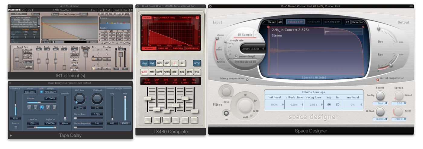
By the end of the 1990s, plug-in reverbs and DAWs were making a real impact on the market. Digital reverb algorithms were now implemented to plugins, and the technology of impulse responses makes it possible to record a “fingerprint” of a room sound, or any hardware reverb, and replicate it via an impulse response reverb plug-in. The most famous one is Altiverb, but these days almost every DAW comes with one (list them). While it is fun to work with original hardware, and there are also great algorithmic reverbs, you can cover most of your needs with impulse response reverbs, but you will of course have to build a library of great impulse responses, and learn how to use them.
Most sought after Reverb Classics
AMS Neve: RMX-16 EMT: 140 Plate, 250, 251 Eventide: SP-2016, H8000 Klark Teknik: DN-780 Lexicon: 480L, 224 (224X, 224XL), 300 (also as 300L with the “LARC”-Remote Control known from the 480L), PCM-70, PCM-60 Quantec: QRS Room Simulator Roland: R-880 Sony: DRE-2000, DRE-S777 (Hardware Impulse Response Reverb, 1999), DPS-V77 Yamaha: REV1, REV5
Bricasti M7 - a 21st century classic
When nobody thought a “new classic reverb” was possible, two former Lexicon-engineers created the Bricasti M7 reverb. Up to this point, the Lexicon 480L was the de facto “industry standard” for professional reverb. It’s successor, the Lexicon 960L, is very powerful, but had disappointed many people who got used to the 480L. Along came the Bricasti M7, and most people pretty much immediately were sold on it. If you really want a hardware unit, this is the one to get.
Your setup for a 3-dimensional mix
The sound of any reverb is highly dependent on the sound source you feed it with. Don’t rely on the same “instant settings” for every mix. What you can do though, is to create a lot of options that can be accessed quickly. The CPU-power of modern computer DAWs makes it easier than ever to access batteries of different reverbs that are set up in a template and can instantly be accessed. If you want to create the impression of a 3-dimensional mix, with lots of space and separation, here are some things to consider: • you need a huge palette of different reverbs and delays, add to that some modulation FX • the reverb you end up using in the mix with will be a mixture of several reverbs that differ in many ways, from colour and density to reverb time • the most important tracks in your mix are accessing completely different reverb and delay sends and returns • you need to have banks of different reverbs ready in your DAW template, specialized for different sources like drum room, snare, toms, lead vocals, pads, lead synth, orchestral instrument • group the reverb returns together with the instruments they belong to - if you have a drum subgroup or VCA group, the reverb returns for the drums belong to that, and exclusively to that • also, you don’t need to create a new send for every reverb - you can send, for example, to 20 different snare reverbs from „Send 5“, and then just unmute and mute them at the aux return, one at a time, until you find what you’re after; this is a very fast and intuitive process, and gives you the option to use one or several reverbs at the same time, and level their balance at the different reverb returns • for subgroups or VCA groups to really work, FX belong mostly exclusively to their sources - if you mute the drum group, you mute all drum reverbs with it, but of course NOT the vocal reverb • it’s essential to stay very organized in that respect All of the above probably sounds like mixes that are drowning in reverb. Don't be fooled - some of these can be very subtle. Also, don't be afraid of long reverb times, but keep them super low in level. Many of these you only hear when you switch them off. Here are some examples for types of reverbs that are useful to have at hand, all at the same time: • most reverbs deliver sounds in traditional categories like plate, chamber, ambience, rooms, concert halls, church reverbs, etc. • most classic reverbs (e.g. Lexicon 224, 480, EMT, AMS RMX) are great at less defined, „cloudy“ reverbs, regardless at which reverb time • modern reverb plug-ins and hardware reverbs (Bricasti M7 is my favourite) are great at super-realistic room simulation • plug-ins using IRs (Impulse Responses) can do both - IRs are basically just samples or „fingerprints“ of the original reverbs or even real rooms What I personally have done over the years was simply try a lot of different reverbs and especially IRs, and everytime I heard something that I liked, I saved the channel strip settings, reverb, EQ and some compression, to a channel strip preset in Logic. Doing this will allow you to keep developing a goto library, and certain reverb chains you can not live without after a while, and these make it to your DAW mix template.
Flavours of Delays
Delays also come in many different flavours: • the typical 1/2, 1/4 or 1/8-note delay „throw“, often used on the last word or syllabel of a vocal-line. • short slap-back delay • super-short microdelays to widen mono signals • complex delays with polyrhythmic patterns, or even unpredicted „weird“ stuff happening in the feedback loop
Philosophical Considerations
Reverbs and delays are to your mix, what a shadow is in a photography, you don’t want them as sharp and shiney as your main object. Most of my delay returns are sending to reverbs as I don’t like them to be a totally dry „sampled“ copy of my original signal. Look at reverbs (and delays) similar to a shadow in a photography, you don't need them 100% upfront, shiny and dynamic, their purpose is to give you a sense of subliminal depth. Compressing them helps that a lot. I also EQ them contrasting to the direct signal for that reason, so if you've worked hard to make your lead vocal upfront, direct and "in your face", you don't want to send your reverb from that direct signal. Compressing reverbs also makes them more controllable - you can get away with less reverb in the mix, if you compress the reverbs that you are using. BTW, this is one reason why older "vintage" reverbs/delays are still popular - they have a low-res, "grainy" feel about them (example Lexicon 224 or AMS DMX1580). Same applies to the character of “tape delays”: because each feedback loop feeds the signal back to the tape head, the saturation effect of analogue tape is very obvious here.
Creating a three-dimensional sound

There are obviously a lot of small details involved, but for a start, get your head around the following concept: important stuff goes to the center: Kick, Bass, Lead Vocals try panning everything else hard left or right Sounds crazy I know. Try panning a guitar hard left, send it to a small room and pan the room hard right. Now bring the reverb a tiny bit more to the center until it feels well-balanced. The second guitar you might have: pan the dry one hard right, send it to another small room (or delay or chorus) and pan the effect hard left. You get the idea… this works for guitars, keyboards, percussions, noise fx, etc. - I use small rooms/chambers/spaces from the Bricasti M7 reverb for that. There are Impulse Responses for the Bricasti out there - for free, and officially authorized by the guys who designed that reverb. To spread stuff out, you can use a super-short delay on some instruments. Logic Pro X has a very useful plug-in called “Sample Delay” that is perfect for that.

Leave one side at 0 ms (original signal bypasses), for the other side try settings under 1000 samples (thats at 44.1k Sample-Rate), values from 300 - 800 work great. Check back and forth in mono, to make sure it doesn’t sound too weird.
Subgroups, FX Busses and Routing

As the number of different reverbs (delays, etc.) you are using grows, you need to keep the routing strictly organized. Using the same reverb on several sources quickly becomes messy. You might need to EQ or compress your main reverb in a certain way to improve its sound on the vocals, but as you have used that same reverb on other instruments you are suddenly affecting the balance and sound of your entire mix. I know it sounds counter-intuitive, but you’re better off separating the reverbs you are using for the different instrument groups, which includes the routing and grouping. On my console, I have a pair of channels dedicated to vocal reverbs, another pair for drum reverbs, and they are assigned to their respective VCA groups. On the drums use pre-fader sends, use the drum fx exclusively for drums, and route their returns to the drum bus as well, and/or put them on the same VCA group. Same goes for parallel compression busses, the sends to them are pre-fader, not following automation, but the returns follow the automation of the source - I do that via the Drum VCA group - you get the added bonus that you can treat the FX returns for each group of instruments separately. We want total control in mixing.
VCA Faders – Balancing the balance.
Balancing the instruments of your song is the essence of mixing. You have a bunch of faders – one for each instrument – and you move ‘em all to a position where your mix sounds great. Easy, right? Well, in theory, thats correct – but there are a bunch of issues that are in the way, such as the following ones, all of which can be resolved by the use of VCA Faders and Groups. Different setups, different problems, same solution. Just a few examples of where VCA Faders and Groups can provide help: • “I don’t even have a mixing console. I do this all in the computer with a mouse.” • “I have a DAW controller with faders, but there is always more tracks than faders.” • “I have the largest SSL console available. But fader 1 and 96 are too far apart. And I only have two hands.” • “The further I progress with my mix, the louder the mix gets, often to the point of distortion. At that point I need to pull all of them down by the same amount. As I’m trying this, the balance also ends up different and I have to start over again.”
Introducing VCA Faders – structure for your mix.
A quick example. You can start a mix by balancing only your drums, then assign all of these drum instruments to the same VCA Fader. Now you are able to control all of the drums with just one fader. The balance you have set will stay intact, and should you need to turn an individual drum instrument up or down, you can still do that, at any time. As a next step, you might add various synthesiser sounds – pads, a lead riff, some melodies – until you got a good balance. The synths are communicating well which each other but once you add vocals you find that the synths are too loud and the drums are collectively too low. At this point you control each group consisting of drums, synths and vocals with just ONE VCA fader each. It definitely makes the mixing process a lot easier. Essentially, a VCA FADER is a fader that controls a group of individual faders, and this VCA GROUP has its own balance within itself. And while the VCA Fader changes the level of each fader in the group proportionally, you can still access the individual faders within the group and make changes to the balance within the VCA GROUP. Essentially, a VCA FADER is a fader that controls a group of individual faders, and this VCA GROUP has its own balance within itself. And while the VCA Fader changes the level of each fader in the group proportionally, you can still access the individual faders within the group and make changes to the balance within the VCA GROUP.
Here’s a quick video of VCA faders in ProTools 12.
If you work with Avid ProTools, Apple Logic Pro X or Steinberg Cubase 8, your DAW has “VCA Faders” or “VCA Groups”. All of these DAW programs have added VCA Faders to the feature list in recent updates. The confusing thing is that earlier versions of Cubase, Logic and ProTools had features that looked similar, but didn’t provide the exact same feature-set as VCA Faders. In other words – the software makers didn’t get it quite right the first time around, and they’re now fixing an old mistake. Unfortunately this shows that the inventors of these programs didn’t really get input from professional mix engineers in the beginning. Ask any pro who has worked with a large analogue console – VCA Faders and Groups were one of THE BIG advantages these always put them ahead of mixing “in the box”. Like many features we enjoy in todays digital DAW world, the functionality of VCA Faders go back to an invention from the analogue world which was essential to the development of early synthesizers like the Minimoog. To fully understand what is going on, let’s get into the details of the underlying analogue technology. What is a VCA? History + Terminology VCA = Voltage Controlled Amplifier
A VCA is an analogue circuit – an amplifier whose volume is controlled by an incoming control voltage.
VCA as used in analogue synthesizers
In a classic analogue synthesizer, for example a Minimoog, the VCA is controlled by an envelope generator – I’m confident you’re familiar with the classic “ADSR”-envelope generator. ADSR stands for “Attack, Decay, Sustain, Release” and describes the volume of a note once triggered by a key on the musical keyboard of an analogue synthesizer (or for that matter, by an incoming MIDI note).

VCA circuit as used in analogue consoles
While the volume of a channel in a mixing console can easily be controlled by running the audio directly through a fader in the mixer which acts as a variable resistor, the manufacturers of professional mixing consoles wanted a more flexibel way to control the volume of each channel. Thats why they added a VCA circuit to each mixer channel (and also the master bus). The VCA circuit could be controlled by any device that would generate the necessary control voltage for the VCA circuit. For example, this could be a range from 0V to 5V which controls the volume from silence to full level. The voltage can be provided from your traditional channel fader, or alternatively by a mix computer that records fader movements and plays them back. The classic SSL mix computer of the E/G-Series consoles is based on this technology. Both the mix computer and the fader of each channel can send a control voltage to the VCA (which is a circuit board located on each mixer channel). The heart of the VCA circuit is a VCA chip. The ones used in the classic SSL consoles were originally manufactured by dbx, and later replaced by VCA chips of manufacturer THATS. If you’re a DIY-nerd, you can purchase those integrated circuits in online electronic shops like Mouser. Different generations of these VCA chips are said to have different audio characteristics, although in theory we want them to sound as neutral as possible. VCA Faders On a classic E/G-Series SSL-Console, EVERY large fader is a VCA-Fader. Audio NEVER passes through the faders – the faders just send a control voltage for the VCA, which can also be recorded to the mix computer in real-time. The mix computer essentially has an A/D and D/A converter which translates and stores the changing voltages for each SMPTE frame of the music’s timeline. Similar to what a DAW does today – only that it records control-voltages instead 24bit audio – not bad for a 1977 computer, right?

VCA Groups
In addition to a fader for each channel, the classic large SSL consoles always had 8 extra faders that control 8 VCA groups. Each large channel fader could be assigned to one of these 8 groups which would (via the VCA group fader) act as a master control for all the channels assigned to each VCA group. Again, no audio signal ever passed through these faders – all they do is provide a control voltage that controls the voltage of the channels according to how they are assigned to the 8 available VCA groups. But there’s a super-tricky thing the SSL console developers invented for the VCA group faders… when the group fader is set to default (= 0dB), they add 0V to the VCA circuits of the assigned groups. If you turn the VCA group fader higher, it adds voltage (= volume) to the channels, if you turn the VCA group fader lower than 0dB, it sends a negative voltage which means it subtracts from the control voltage so all assigned VCAs reduce their relative volume by the same perceived amount. Very simple but effective!
VCA Trim
The use of VCAs in analogue consoles would solve another very common problem every user of analogue consoles would frequently run across. Remember how you sometimes end up pushing all faders higher and higher, and at one point overload your master bus? This is where the “VCA trim” comes into play… it’s basically just one knob that globally adds or subtracts voltage to ALL VCAs in the system.
When to use what.
Audio Subgroups
The most basic audio subgroup every mixer and DAW software has is the Stereobus. But more commonly, we associate audio subgroups with a routing where a number of tracks are submixed before these different groups get summed together in the Stereobus. Audio Subgroups are great for situations when you want to “glue” various elements together with processors like compressors and saturators, or you want to apply similar reverbs on all of them at the same time. A Drum-Subgroup is a great example for the “glue”-situation, where as a subgroup for Backing Vocals is very convenient to add the same kind of Reverb FX on all of them at once. If all you want to do is have one fader for ALL the drums, or ALL the vocals, but your not planning on any “group” processing, you’re better off using VCA Faders.
Fader Groups
When several faders in your mixer are “linked”, many DAWs call this a “Fader Group” or “Fader Link”. The individual faders can have different levels, but they are all linked. When you bring one fader up, the others are brought up as well, proportional to their original settings. Many early DAWs had this feature, but as soon as you wanted to change one of the faders within the group, but not the others, you had to temporarily remove this one fader from the Fader group, change the level, then add it to the group again. Which is of course doable, but not convenient and definitely preventing “intuitive” changes “on the fly”.
VCA Faders
VCA Faders are very similar to “Fader Groups” with the only difference being that you can change the individual level of every fader at any time while they still remain linked to the “fader group”.
How to create a VCA-Fader stack.
Logic Pro X
Select the tracks you want to group to a VCA fader. Then use “Create Track Stack”.
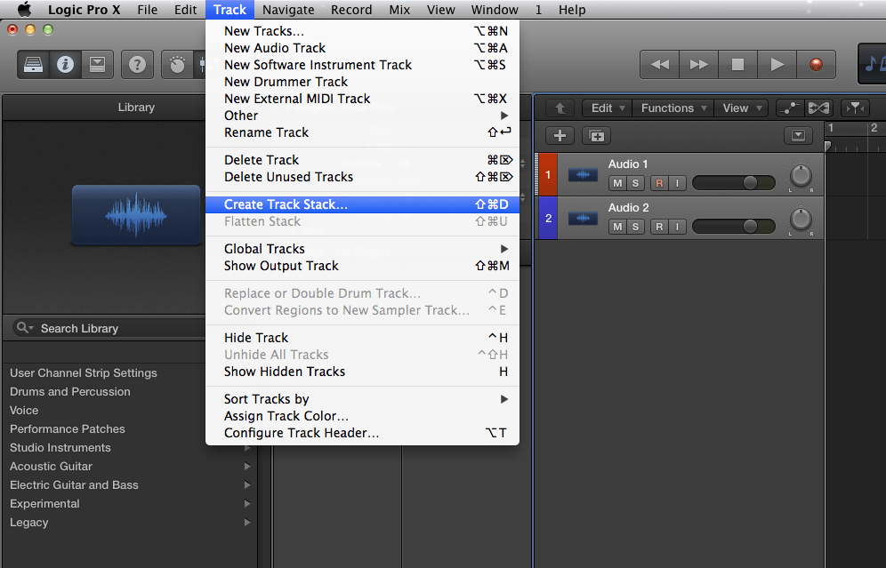
Now you pick “Folder Stack” for the VCA function.” Summing Stack” will create an extra bus for summing.

ProTools 12
First you have to create a new track.
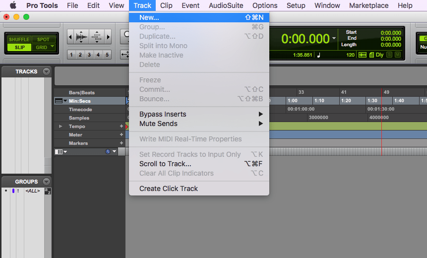
Select “VCA Master” to create a new VCA fader.

Then you can add audio tracks to you session.

Finally group them to the VCA fader you already set up.
 Cubase 8
Open the mixer window and select the track you want to group to a VCA fader. Then right-click on them and pick “Add VCA Fader to Selected Channels”.

The new VCA fader will control the selected tracks now

+++++++++++++++++++++++++++++++++++++++++++++++++++++++++++++++++
e- Mixing Information and data so do control
++++++++++++++++++++++++++++++++++++++++++++++++++++++++++++++++
Tidak ada komentar:
Posting Komentar