Tuning the Economy and tune working capital to electronic economics

I.  General Theory of Employment, Interest and Money to argue that in a depression the government should expand G to increase aggregate demand in order to stimulate the economy back to a state of full employment. the  government could fine tune the economy in order to eliminate the business cycle all together. Consider the following graph:


 

 During the period that the actual GDP is above the GDP trend meaning that the economy is overheated and runs the risk of demand push inflation the government should run a surplus. During a recession when the actual GDP is below the GDP trend the government spends the accumulated surplus to stimulate the economy. Over the business cycle there is no debt. 
example problem : Besides the problem of timing there is a basic political problem in fine tuning the economy . Legislators and the President want to get reelected. Before the tax cut , politicians believed they were obligate to balance the budget . They interpreted Keynesian fine tuning in their self interests of wanting to get reelected and assumed that they never had to balance the budget since given goodies to constituents would get them reelected and such actions could be justified by their interpretation of Keynes. Remember Keyes proposed his policies for a depression not for fine tuning the economy. 
The central tenet of this school of thought is that government intervention can stabilize the economy
Just how important is money? Few would deny that it plays a key role in the economy.­
During the Great Depression of the 1930s, existing economic theory was unable either to explain the causes of the severe worldwide economic collapse or to provide an adequate public policy solution to jump-start production and employment.
British economist John Maynard Keynes spearheaded a revolution in economic thinking that overturned the then-prevailing idea that free markets would automatically provide full employment—that is, that everyone who wanted a job would have one as long as workers were flexible in their wage demands (see box). The main plank of Keynes’s theory, which has come to bear his name, is the assertion that aggregate demand—measured as the sum of spending by households, businesses, and the government—is the most important driving force in an economy. Keynes further asserted that free markets have no self-balancing mechanisms that lead to full employment. Keynesian economists justify government intervention through public policies that aim to achieve full employment and price stability.

The revolutionary idea

Keynes argued that inadequate overall demand could lead to prolonged periods of high unemployment. An economy’s output of goods and services is the sum of four components: consumption, investment, government purchases, and net exports (the difference between what a country sells to and buys from foreign countries). Any increase in demand has to come from one of these four components. But during a recession, strong forces often dampen demand as spending goes down. For example, during economic downturns uncertainty often erodes consumer confidence, causing them to reduce their spending, especially on discretionary purchases like a house or a car. This reduction in spending by consumers can result in less investment spending by businesses, as firms respond to weakened demand for their products. This puts the task of increasing output on the shoulders of the government. According to Keynesian economics, state intervention is necessary to moderate the booms and busts in economic activity, otherwise known as the business cycle.



II. Tuning working capital
  


Walgreen's represents our normal case and arguably shows the best practice in this regard: the company uses LIFO inventory costing, and its LIFO reserve increases year over year. In a period of rising prices, LIFO will assign higher prices to the consumed inventory (cost of goods sold) and is therefore more conservative. Just as COGS on the income statement tends to be higher under LIFO than under FIFO, the inventory account on the balance sheet tends to be understated. For this reason, companies using LIFO must disclose (usually in a footnote) a LIFO reserve, which when added to the inventory balance as reported, gives the FIFO-equivalent inventory balance.

Because GAP Incorporated uses FIFO inventory costing, there is no need for a "LIFO reserve." However, GAP's and Walgreen's gross profit margins are not commensurable. In other words, comparing FIFO to LIFO is not like comparing apples to apples. GAP will get a slight upward bump to its gross profit margin because its inventory method will tend to undercount the cost of goods. There is no automatic solution for this. Rather, we can revise GAP's COGS (in dollar terms) if we make an assumption about the inflation rate during the year. Specifically, if we assume that the inflation rate for the inventory was R% during the year, and if "Inventory Beginning" in the equation below equals the inventory balance under FIFO, we can re-estimate COGS under LIFO with the following equation:



Kohl's Corporation uses LIFO, but its LIFO reserve declined year over year - from $4.98 million to zero. This is known as LIFO liquidation or liquidation of LIFO layers, and indicates that during the fiscal year, Kohl's sold or liquidated inventory that was held at the beginning of the year. When prices are rising, we know that inventory held at the beginning of the year carries a lower cost (because it was purchased in prior years). Cost of goods sold is therefore reduced, sometimes significantly. Generally, in the case of a sharply declining LIFO reserve, we can assume that reported profit margins are upwardly biased to the point of distortion.

Cash Conversion Cycle The cash conversion cycle is a measure of working capital efficiency, often giving valuable clues about the underlying health of a business. The cycle measures the average number of days that working capital is invested in the operating cycle. It starts by adding days inventory outstanding (DIO) to days sales outstanding (DSO). This is because a company "invests" its cash to acquire/build inventory, but does not collect cash until the inventory is sold and the accounts receivable are finally collected.

Receivables are essentially loans extended to customers that consume working capital; therefore, greater levels of DIO and DSO consume more working capital. However, days payable outstanding (DPO), which essentially represent loans from vendors to the company, are subtracted to help offset working capital needs. In summary, the cash conversion cycle is measured in days and equals DIO + DSO – DPO:



Here we extracted two lines from Kohl's (a retail department store) most recent income statement and a few lines from their working capital accounts.


Circled in green are the accounts needed to calculate the cash conversion cycle. From the income statement, you need net sales and COGS. From the balance sheet, you need receivables, inventories and payables. Below, we show the two-step calculation. First, we calculate the three turnover ratios: receivables turnover (sales/average receivables), inventory turnover (COGS/average inventory) and payables turnover (purchases/average payables). The turnover ratios divide into an average balance because the numerators (such as sales in the receivables turnover) are flow measures over the entire year.

Also, for payables turnover, some use COGS/average payables. That's okay, but it's slightly more accurate to divide average payables into purchases, which equals COGS plus the increase in inventory over the year (inventory at end of year minus inventory at beginning of the year). This is better because payables finance all of the operating dollars spent during the period (that is, they are credit extended to the company). And operating dollars, in addition to COGS, may be spent to increase inventory levels.

The turnover ratios do not mean much in isolation; they are used to compare one company to another. But if you divide the turnover ratios into 365 (for example, 365/receivables turnover), you get the "days outstanding" numbers. Below, for example, a receivable turnover of 9.6 becomes 38 days sales outstanding (DSO). This number has more meaning; it means that, on average, Kohl's collects its receivables in 38 days.


Here is a graphic summary of Kohl's cash conversion cycle for 2003. On average, working capital spent 92 days in Kohl's operating cycle:


Let's contrast Kohl's with Limited Brands. Below we perform the same calculations in order to determine the cash conversion cycle for Limited Brands:

While Kohl's cycle is 92 days, Limited Brand's cycle is only 37. Why does this matter? Because working capital must be financed somehow, with either debt or equity, and both companies use debt. Kohl's cost of sales (COGS) is about $6.887 billion per year, or almost $18.9 million per day ($6.887 billion/365 days). Because Kohl's cycle is 92 days, it must finance--that is, fund its working capital needs--to the tune of about $1.7+ billion per year ($18.9 million x 92 days). If interest on its debt is 5%, then the cost of this financing is about $86.8 million ($1.7 billion x 5%) per year. However, if, hypothetically, Kohl's were able to reduce its cash conversion cycle to 37 days--the length of Limited Brands' cycle--its cost of financing would drop to about $35 million ($18.9 million per day x 37 days x 5%) per year. In this way, a reduction in the cash conversion cycle drops directly to the bottom line.

But even better, the year over year trend in the cash conversion cycle often serves as a sign of business health or deterioration. Declining DSO means customers are paying sooner; conversely, increasing DSO could mean the company is using credit to push product. A declining DIO signifies that inventory is moving out rather than "piling up." Finally, some analysts believe that an increasing DPO is a signal of increasing economic leverage in the marketplace. The textbook examples here are Walmart and Dell: these companies can basically dictate the terms of their relationships to their vendors and, in the process, extend their days payable (DPO).

Looking "Under the Hood" for Other Items
Most of the other working capital accounts are straightforward, especially the current liabilities side of the balance sheet. But you do want to be on the alert for the following:

• Off-balance-sheet financing
• Derivatives

For examples of these two items, consider the current assets section of Delta Airlines' fiscal year 2003 balance sheet:


Notice that Delta's receivables more than doubled from 2002 to 2003. Is this a dangerous sign of collections problems? Let's take a look at the footnote:

We were party to an agreement, as amended, under which we sold a defined pool of our accounts receivable, on a revolving basis, through a special-purpose, wholly owned subsidiary, which then sold an undivided interest in the receivables to a third party.... This agreement terminated on its scheduled expiration date of March 31, 2003. As a result, on April 2, 2003, we paid $250 million, which represented the total amount owed to the third party by the subsidiary, and subsequently collected the related receivables. (Note 8, Delta 10-K FY 2003)

Here's the translation: during 2002, most of Delta's receivables were factored in an off-balance sheet transaction. By factored, we mean Delta sold some of its accounts receivables to another company (via a subsidiary) in exchange for cash. In brief, Delta gets paid quickly rather than having to wait for customers to pay. However, the seller (Delta in this case) typically retains some or all of the credit risk - the risk that customers will not pay. For example, they may collateralize the receivables.

We see that during 2003, the factored receivables were put back onto the balance sheet. In economic terms, they never really left but sort of disappeared in 2002. So the 2003 number is generally okay, but there was not a dramatic jump. More importantly, if we were to analyze year 2002, we'd have to be sure to manually "add-back" the off-balance sheet receivables, which would otherwise look artificially favorable for that year.

We also highlighted Delta's increase in "prepaid expenses and other" because this innocent-looking account contains the fair value of Delta's fuel hedge derivatives. Here's what the footnote says:

Prepaid expenses and other current assets increased by 34%, or $120 million, primarily due to an increase in prepaid aircraft fuel as well as an increase in the fair value of our fuel hedge derivative contracts.... Approximately 65%, 56% and 58% of our aircraft fuel requirements were hedged during 2003, 2002 and 2001, respectively. In February 2004, we settled all of our fuel hedge contracts prior to their scheduled settlement dates… and none of our projected aircraft fuel requirements for 2005 or thereafter.

The rules concerning derivatives are complex, but the idea is this: it is entirely likely that working capital accounts contain embedded derivative instruments. In fact, the basic rule is that, if a derivative is a hedge whose purpose is to mitigate risk (as opposed to a hedge whose purpose is to speculate), then the value of the hedge will impact the carrying value of the hedged asset. For example, if fuel oil is an inventory item for Delta, then derivatives contracts meant to lock-in future fuel oil costs will directly impact the inventory balance. Most derivatives, in fact, are not used to speculate but rather to mitigate risks that the company cannot control.

Delta's footnote above has good news and bad news. The good news is that as fuel prices rose, the company made some money on its fuel hedges, which in turn offset the increase in fuel prices - the whole point of their design! But this is overshadowed by news which is entirely bad: Delta settled "all of [their] fuel hedge contracts" and has no hedges in place for 2005 and thereafter! Delta is thus exposed in the case of high fuel prices, which is a serious risk factor for the stock.

Summary Traditional analysis of working capital is defensive; it asks, "Can the company meet its short-term cash obligations?" But working capital accounts also tell you about the operational efficiency of the company. The length of the cash conversion cycle (DSO+DIO-DPO) tells you how much working capital is tied up in ongoing operations. And trends in each of the days-outstanding numbers may foretell improvements or declines in the health of the business.

Investors should check the inventory costing method, and LIFO is generally preferred to FIFO. However, if the LIFO reserve drops precipitously year over year, then the implied inventory liquidation distorts COGS and probably renders the reported profit margin unusable.

Finally, it's wise to check the current accounts for derivatives (or the lack of them, when key risks exist) and off-balance sheet financing.



    
III . Tuning Electronic Economics




    

• Addresses new economic issues and problems that are arising as more and more transactions are conducted electronically
• Explores the emerging network-based, real-time macroeconomy with its own set of economic characteristics
• Covers such topics as pricing schemes for electronic services, electronic trading systems, data mining and high-frequency data, real-time forecasting, filtering, etc.

The journal Netnomics is intended to be an outlet for research in electronic networking as well as in network economics.
As more and more transactions are carried out electronically, important economic issues and problems arise. A network-based real-time macroeconomy has emerged with its own set of economic characteristics, creating a wealth of opportunities for economic research as well as important linkages to information systems. Topics that could be addressed are pricing schemes for electronic services, electronic trading systems, data mining and high-frequency online data as well as big data, real-time forecasting, filtering, economic software agents, distributed database applications, electronic money and tickets, and many more. Evidently, this is only the tip of the iceberg. Moreover, we attempt to disclose important research questions in the field of network economics. This may reflect networks in their widest sense regarding,
for instance, telecommunications, electronic networks, supply chain networks, networks in traffic and transportation such as the airline and maritime shipping industries, or even electricity networks and smart grids. Papers of Netnomics describe cutting edge research and applications in these areas.





  
   

blocking theory for control of closed and open control on mathematical calculations and computer electronics equipment in the future as well as the means of measurement tools in the variables x, y, z ..... etc

The theoretical basis of blocking is the following mathematical result. Given random variables, X and Y

    \operatorname{Var}(X-Y)= \operatorname{Var}(X) + \operatorname{Var}(Y) - 2\operatorname{Cov}(X,Y).

The difference between the treatment and the control can thus be given minimum variance (i.e. maximum precision) by maximising the covariance (or the correlation) between X and Y. 




This reduces sources of variability and thus leads to greater precision.
Use

Reducing known variability is exactly what blocking does. Its principle lies in the fact that a variability that cannot be overcome (e.g. needing two batches of raw material to produce 1 container of a chemical) is confounded or aliased with a(n) (higher/highest order) interaction to eliminate its influence on the end product. High order interactions are usually of the least importance (think of the fact that temperature of a reactor or the batch of raw materials is more important than the combination of the two - this is especially true when more (3, 4, ...) factors are present) thus it is preferable to confound this variability with the higher interaction.

Suppose a process is invented that intends to make the soles of shoes last longer, and a plan is formed to conduct a field trial. Given a group of n volunteers, one possible design would be to give n/2 of them shoes with the new soles and n/2 of them shoes with the ordinary soles, randomizing the assignment of the two kinds of soles. This type of experiment is a completely randomized design. Both groups are then asked to use their shoes for a period of time, and then measure the degree of wear of the soles. This is a workable experimental design, but purely from the point of view of statistical accuracy (ignoring any other factors), a better design would be to give each person one regular sole and one new sole, randomly assigning the two types to the left and right shoe of each volunteer. Such a design is called a randomized complete block design. This design will be more sensitive than the first, because each person is acting as their own control and thus the control group is more closely matched to the treatment group.
Theoretical basis 


blocking instance variable  


The design of experiments (DOE, DOX, or experimental design) is the design of any task that aims to describe or explain the variation of information under conditions that are hypothesized to reflect the variation. The term is generally associated with true experiments in which the design introduces conditions that directly affect the variation, but may also refer to the design of quasi-experiments, in which natural conditions that influence the variation are selected for observation.
In its simplest form, an experiment aims at predicting the outcome by introducing a change of the preconditions, which is reflected in a variable called the predictor. The change in the predictor is generally hypothesized to result in a change in the second variable, hence called the outcome variable. Experimental design involves not only the selection of suitable predictors and outcomes, but planning the delivery of the experiment under statistically optimal conditions given the constraints of available resources.
Main concerns in experimental design include the establishment of validity, reliability, and replicability. For example, these concerns can be partially addressed by carefully choosing the predictor, reducing the risk of measurement error, and ensuring that the documentation of the method is sufficiently detailed. Related concerns include achieving appropriate levels of statistical power and sensitivity.
Correctly designed experiments advance knowledge in the natural and social sciences and engineering. Other applications include marketing and policy making. 



  Lind limited his subjects to men who "were as similar as I could have them", that is he provided strict entry requirements to reduce extraneous variation. He divided them into six pairs, giving each pair different supplements to their basic diet for two weeks. The treatments were all remedies that had been proposed:

• A quart of cider every day.
• Twenty five gutts (drops) of vitriol (sulphuric acid) three times a day upon an empty stomach.
• One half-pint of seawater every day.
• A mixture of garlic, mustard, and horseradish in a lump the size of a nutmeg.
• Two spoonfuls of vinegar three times a day.
• Two oranges and one lemon every day.

The citrus treatment stopped after six days when they ran out of fruit, but by that time one sailor was fit for duty while the other had almost recovered. Apart from that, only group one (cider) showed some effect of its treatment. The remainder of the crew presumably served as a control, but Lind did not report results from any control (untreated) group 

A methodology for designing experiments was proposed by Ronald Fisher, in his innovative books: The Arrangement of Field Experiments (1926) and The Design of Experiments (1935). Much of his pioneering work dealt with agricultural applications of statistical methods. As a mundane example, he described how to test the lady tasting tea hypothesis, that a certain lady could distinguish by flavour alone whether the milk or the tea was first placed in the cup. These methods have been broadly adapted in the physical and social sciences, are still used in agricultural engineering and differ from the design and analysis of computer experiments.

Comparison

In some fields of study it is not possible to have independent measurements to a traceable metrology standard. Comparisons between treatments are much more valuable and are usually preferable, and often compared against a scientific control or traditional treatment that acts as baseline.

Randomization

Random assignment is the process of assigning individuals at random to groups or to different groups in an experiment, so that each individual of the population has the same chance of becoming a participant in the study. The random assignment of individuals to groups (or conditions within a group) distinguishes a rigorous, "true" experiment from an observational study or "quasi-experiment".^[12] There is an extensive body of mathematical theory that explores the consequences of making the allocation of units to treatments by means of some random mechanism such as tables of random numbers, or the use of randomization devices such as playing cards or dice. Assigning units to treatments at random tends to mitigate confounding, which makes effects due to factors other than the treatment to appear to result from the treatment. The risks associated with random allocation (such as having a serious imbalance in a key characteristic between a treatment group and a control group) are calculable and hence can be managed down to an acceptable level by using enough experimental units. However, if the population is divided into several subpopulations that somehow differ, and the research requires each subpopulation to be equal in size, stratified sampling can be used. In that way, the units in each subpopulation are randomized, but not the whole sample. The results of an experiment can be generalized reliably from the experimental units to a larger statistical population of units only if the experimental units are a random sample from the larger population; the probable error of such an extrapolation depends on the sample size, among other things.

Statistical replication

Measurements are usually subject to variation and measurement uncertainty; thus they are repeated and full experiments are replicated to help identify the sources of variation, to better estimate the true effects of treatments, to further strengthen the experiment's reliability and validity, and to add to the existing knowledge of the topic.^[13] However, certain conditions must be met before the replication of the experiment is commenced: the original research question has been published in a peer-reviewed journal or widely cited, the researcher is independent of the original experiment, the researcher must first try to replicate the original findings using the original data, and the write-up should state that the study conducted is a replication study that tried to follow the original study as strictly as possible.^[14]

Blocking

Blocking is the arrangement of experimental units into groups (blocks/lots) consisting of units that are similar to one another. Blocking reduces known but irrelevant sources of variation between units and thus allows greater precision in the estimation of the source of variation under study.

Orthogonality

Example of orthogonal factorial design

Orthogonality concerns the forms of comparison (contrasts) that can be legitimately and efficiently carried out. Contrasts can be represented by vectors and sets of orthogonal contrasts are uncorrelated and independently distributed if the data are normal. Because of this independence, each orthogonal treatment provides different information to the others. If there are T treatments and T – 1 orthogonal contrasts, all the information that can be captured from the experiment is obtainable from the set of contrasts.

Factorial experiments

Use of factorial experiments instead of the one-factor-at-a-time method. These are efficient at evaluating the effects and possible interactions of several factors (independent variables). Analysis of experiment design is built on the foundation of the analysis of variance, a collection of models that partition the observed variance into components, according to what factors the experiment must estimate or test.  

This example is attributed to Harold Hotelling.It conveys some of the flavor of those aspects of the subject that involve combinatorial designs.
Weights of eight objects are measured using a pan balance and set of standard weights. Each weighing measures the weight difference between objects in the left pan vs. any objects in the right pan by adding calibrated weights to the lighter pan until the balance is in equilibrium. Each measurement has a random error. The average error is zero; the standard deviations of the probability distribution of the errors is the same number σ on different weighings; and errors on different weighings are independent. Denote the true weights by

We consider two different experiments:

1. Weigh each object in one pan, with the other pan empty. Let X_i be the measured weight of the object, for i = 1, ..., 8.
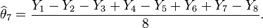
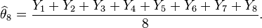
2. Do the eight weighings according to the following schedule and let Y_i be the measured difference for i = 1, ..., 8:

Then the estimated value of the weight θ₁ is

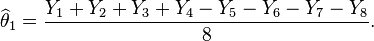
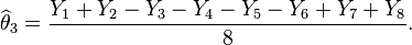
Similar estimates can be found for the weights of the other items. For example

The question of design of experiments is: which experiment is better?
The variance of the estimate X₁ of θ₁ is σ² if we use the first experiment. But if we use the second experiment, the variance of the estimate given above is σ²/8. Thus the second experiment gives us 8 times as much precision for the estimate of a single item, and estimates all items simultaneously, with the same precision. What the second experiment achieves with eight would require 64 weighings if the items are weighed separately. However, note that the estimates for the items obtained in the second experiment have errors that correlate with each other.
Many problems of the design of experiments involve combinatorial designs, as in this example and others.

Avoiding false positives

False positive conclusions, often resulting from the pressure to publish or the author's own confirmation bias, are an inherent hazard in many fields. A good way to prevent biases potentially leading to false positives in the data collection phase is to use a double-blind design. When a double-blind design is used, participants are randomly assigned to experimental groups but the researcher is unaware of what participants belong to which group. Therefore, the researcher can not affect the participants' response to the intervention. Experimental designs with undisclosed degrees of freedom are a problem. This can lead to conscious or unconscious "p-hacking": trying multiple things until you get the desired result. It typically involves the manipulation - perhaps unconsciously - of the process of statistical analysis and the degrees of freedom until they return a figure below the p<.05 level of statistical significance. So the design of the experiment should include a clear statement proposing the analyses to be undertaken. P-hacking can be prevented by preregistering researches, in which researchers have to send their data analysis plan to the journal they wish to publish their paper in before they even start their data collection, so no data mining is possible . Another way to prevent this is taking the double-blind design to the data-analysis phase, where the data are sent to a data-analyst unrelated to the research who scrambles up the data so there is no way to know which participants belong to before they are potentially taken away as outliers.
Clear and complete documentation of the experimental methodology is also important in order to support replication of results.

Discussion topics when setting up an experimental design

An experimental design or randomized clinical trial requires careful consideration of several factors before actually doing the experiment. An experimental design is the laying out of a detailed experimental plan in advance of doing the experiment. Some of the following topics have already been discussed in the principles of experimental design section:

1. How many factors does the design have? and are the levels of these factors fixed or random?
2. Are control conditions needed, and what should they be?
3. Manipulation checks; did the manipulation really work?
4. What are the background variables?
5. What is the sample size. How many units must be collected for the experiment to be generalisable and have enough power?
6. What is the relevance of interactions between factors?
7. What is the influence of delayed effects of substantive factors on outcomes?
8. How do response shifts affect self-report measures?
9. How feasible is repeated administration of the same measurement instruments to the same units at different occasions, with a post-test and follow-up tests?
10. What about using a proxy pretest?
11. Are there lurking variables?
12. Should the client/patient, researcher or even the analyst of the data be blind to conditions?
13. What is the feasibility of subsequent application of different conditions to the same units?
14. How many of each control and noise factors should be taken into account?

The independent variable of a study often has many levels or different groups. In a true experiment, researchers can have an experimental group, which is where their intervention testing the hypothesis is implemented, and a control group, which has all the same element as the experimental group, without the interventional element. Thus, when everything else except for one intervention is held constant, researchers can certify with some certainty that this one element is what caused the observed change. In some instances, having a control group is not ethical. This is sometimes solved using two different experimental groups. In some cases, independent variables are not manipulable, for example when testing the difference between two groups who have a different disease, or testing the difference between genders (obviously variables that would be hard or unethical to assign participants to). In these cases, a quasi-experimental design may be used.

Causal attributions

In the pure experimental design, the independent (predictor) variable is manipulated by the researcher - that is - every participant of the research is chosen randomly from the population, and each participant chosen is assigned randomly to conditions of the independent variable. Only when this is done is it possible to certify with high probability that the reason for the differences in the outcome variables are caused by the different conditions. Therefore, researchers should choose the experimental design over other design types whenever possible. However, the nature of the independent variable does not always allow for manipulation. In those cases, researchers must be aware of not certifying about causal attribution when their design doesn't allow for it. For example, in observational designs, participants are not assigned randomly to conditions, and so if there are differences found in outcome variables between conditions, it is likely that there is something other than the differences between the conditions that causes the differences in outcomes, that is - a third variable. The same goes for studies with correlational design. (Adér & Mellenbergh, 2008).

Statistical control

It is best that a process be in reasonable statistical control prior to conducting designed experiments. When this is not possible, proper blocking, replication, and randomization allow for the careful conduct of designed experiments. To control for nuisance variables, researchers institute control checks as additional measures. Investigators should ensure that uncontrolled influences (e.g., source credibility perception) do not skew the findings of the study. A manipulation check is one example of a control check. Manipulation checks allow investigators to isolate the chief variables to strengthen support that these variables are operating as planned.
One of the most important requirements of experimental research designs is the necessity of eliminating the effects of spurious, intervening, and antecedent variables. In the most basic model, cause (X) leads to effect (Y). But there could be a third variable (Z) that influences (Y), and X might not be the true cause at all. Z is said to be a spurious variable and must be controlled for. The same is true for intervening variables (a variable in between the supposed cause (X) and the effect (Y)), and anteceding variables (a variable prior to the supposed cause (X) that is the true cause). When a third variable is involved and has not been controlled for, the relation is said to be a zero order^{[disambiguation needed]} relationship. In most practical applications of experimental research designs there are several causes (X1, X2, X3). In most designs, only one of these causes is manipulated at a time.

Experimental designs after Fisher

Some efficient designs for estimating several main effects were found independently and in near succession by Raj Chandra Bose and K. Kishen in 1940 at the Indian Statistical Institute, but remained little known until the Plackett-Burman designs were published in Biometrika in 1946. About the same time, C. R. Rao introduced the concepts of orthogonal arrays as experimental designs. This concept played a central role in the development of Taguchi methods by Genichi Taguchi, which took place during his visit to Indian Statistical Institute in early 1950s. His methods were successfully applied and adopted by Japanese and Indian industries and subsequently were also embraced by US industry albeit with some reservations.
In 1950, Gertrude Mary Cox and William Gemmell Cochran published the book Experimental Designs, which became the major reference work on the design of experiments for statisticians for years afterwards.
Developments of the theory of linear models have encompassed and surpassed the cases that concerned early writers. Today, the theory rests on advanced topics in linear algebra, algebra and combinatorics.
As with other branches of statistics, experimental design is pursued using both frequentist and Bayesian approaches: In evaluating statistical procedures like experimental designs, frequentist statistics studies the sampling distribution while Bayesian statistics updates a probability distribution on the parameter space.

Human participant experimental design constraints

 

Laws and ethical considerations preclude some carefully designed experiments with human subjects. Legal constraints are dependent on jurisdiction. Constraints may involve institutional review boards, informed consent and confidentiality affecting both clinical (medical) trials and behavioral and social science experiments. In the field of toxicology, for example, experimentation is performed on laboratory animals with the goal of defining safe exposure limits for humans.Balancing the constraints are views from the medical field. Regarding the randomization of patients, "... if no one knows which therapy is better, there is no ethical imperative to use one therapy or another." (p 380) Regarding experimental design, "...it is clearly not ethical to place subjects at risk to collect data in a poorly designed study when this situation can be easily avoided...". (p 393) 

Plackett–Burman designs are experimental designs presented in 1946 by Robin L. Plackett and J. P. Burman while working in the British Ministry of Supply. Their goal was to find experimental designs for investigating the dependence of some measured quantity on a number of independent variables (factors), each taking L levels, in such a way as to minimize the variance of the estimates of these dependencies using a limited number of experiments. Interactions between the factors were considered negligible. The solution to this problem is to find an experimental design where each combination of levels for any pair of factors appears the same number of times, throughout all the experimental runs (refer table). A complete factorial design would satisfy this criterion, but the idea was to find smaller designs.

Plackett–Burman design for 12 runs and 11 two-level factors^[2] For any two X_i, each combination ( --, -+, +-, ++) appears three - i.e. the same number of times.

Run	X1	X2	X3	X4	X5	X6	X7	X8	X9	X10	X11
1	+	+	+	+	+	+	+	+	+	+	+
2	−	+	−	+	+	+	−	−	−	+	−
3	−	−	+	−	+	+	+	−	−	−	+
4	+	−	−	+	−	+	+	+	−	−	−
5	−	+	−	−	+	−	+	+	+	−	−
6	−	−	+	−	−	+	−	+	+	+	−
7	−	−	−	+	−	−	+	−	+	+	+
8	+	−	−	−	+	−	−	+	−	+	+
9	+	+	−	−	−	+	−	−	+	−	+
10	+	+	+	−	−	−	+	−	−	+	−
11	−	+	+	+	−	−	−	+	−	−	+
12	+	−	+	+	+	−	−	−	+	−	−

For the case of two levels (L=2), Plackett and Burman used the method found in 1933 by Raymond Paley for generating orthogonal matrices whose elements are all either 1 or -1 (Hadamard matrices). Paley's method could be used to find such matrices of size N for most N equal to a multiple of 4. In particular, it worked for all such N up to 100 except N = 92. If N is a power of 2, however, the resulting design is identical to a fractional factorial design, so Plackett–Burman designs are mostly used when N is a multiple of 4 but not a power of 2 (i.e. N = 12, 20, 24, 28, 36 …). If one is trying to estimate less than N parameters (including the overall average), then one simply uses a subset of the columns of the matrix.
For the case of more than two levels, Plackett and Burman rediscovered designs that had previously been given by Raj Chandra Bose and K. Kishen at the Indian Statistical Institute.^[4] Plackett and Burman give specifics for designs having a number of experiments equal to the number of levels L to some integer power, for L = 3, 4, 5, or 7.
When interactions between factors are not negligible, they are often confounded in Plackett–Burman designs with the main effects, meaning that the designs do not permit one to distinguish between certain main effects and certain interactions. This is called aliasing or confounding.

Extended uses

In 1993, Dennis Lin described a construction method via half-fractions of Plackett-Burman designs, using one column to take half of the rest of the columns. The resulting matrix, minus that column, is a "supersaturated design" for finding significant first order effects, under the assumption that few exist.
Box-Behnken designs can be made smaller, or very large ones constructed, by replacing the fractional factorials and incomplete blocks traditionally used for plan and seed matrices, respectively, with Plackett-Burmans. For example, a quadratic design for 30 variables requires a 30 column PB plan matrix of zeroes and ones, replacing the ones in each line using PB seed matrices of -1s and +1s (for 15 or 16 variables) wherever a one appears in the plan matrix, creating a 557 runs design with values, -1, 0, +1, to estimate the 496 parameters of a full quadratic model.
By equivocating certain columns with parameters to be estimated, Plackett-Burmans can also be used to construct mixed categorical and numerical designs, with interactions or high order effects, requiring no more than 4 runs more than the number of model parameters to be estimated. Sort on columns assigned to categorical variable "A", defined as A = 1+int(a*i /(max(i)+.00001)) where i is row number and a is A's number of values. Next sort on columns assigned to any other categorical variables and repeat as needed. Such designs, if large, may otherwise be incomputable by standard search techniques like D-Optimality. For example, 13 variables averaging 3 values each could have well over a million combinations to search. To estimate roughly 100 parameters for a nonlinear model in 13 variables must formally exclude from consideration or compute |X'X| for well over 10⁶C10² or roughly 10⁶⁰⁰ matrices.


Computer simulations are constructed to emulate a physical system. Because these are meant to replicate some aspect of a system in detail, they often do not yield an analytic solution. Therefore, methods such as discrete event simulation or finite element solvers are used. A computer model is used to make inferences about the system it replicates. For example, climate models are often used because experimentation on an earth sized object is impossible.

Objectives

Computer experiments have been employed with many purposes in mind. Some of those include:

• Uncertainty quantification: Characterize the uncertainty present in a computer simulation arising from unknowns during the computer simulation's construction.
• Inverse problems: Discover the underlying properties of the system from the physical data.
• Bias correction: Use physical data to correct for bias in the simulation.
• Data assimilation: Combine multiple simulations and physical data sources into a complete predictive model.
• Systems design: Find inputs that result in optimal system performance measures.

Computer simulation modeling

 

 

Modeling of computer experiments typically uses a Bayesian framework. Bayesian statistics is an interpretation of the field of statistics where which all evidence about the true state of the world is explicitly expressed in the form of probabilities. In the realm of computer experiments, the Bayesian interpretation would imply we must form a prior distribution that represents our prior belief on the structure of the computer model. The use of this philosophy for computer experiments started in the 1980s and is nicely summarized by Sacks et al. (1989) . While the Bayesian approach is widely used, frequentist approaches have been recently discussed .
The basic idea of this framework is to model the computer simulation as an unknown function of a set of inputs. The computer simulation is implemented as a piece of computer code that can be evaluated to produce a collection of outputs. Examples of inputs to these simulations are coefficients in the underlying model, initial conditions and forcing functions. It is natural to see the simulation as a deterministic function that maps these inputs into a collection of outputs. On the basis of seeing our simulator this way, it is common to refer to the collection of inputs as , the computer simulation itself as , and the resulting output as . Both and are vector quantities, and they can be very large collections of values, often indexed by space, or by time, or by both space and time.
Although is known in principle, in practice this is not the case. Many simulators comprise tens of thousands of lines of high-level computer code, which is not accessible to intuition. For some simulations, such as climate models, evaluation of the output for a single set of inputs can require millions of computer hours .

Gaussian process prior

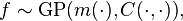
The typical model for a computer code output is a Gaussian process. For notational simplicity, assume is a scalar. Owing to the Bayesian framework, we fix our belief that the function follows a Gaussian process, where is the mean function and is the covariance function. Popular mean functions are low order polynomials and a popular covariance function is Matern covariance, which includes both the exponential () and Gaussian covariances (as ).

Design of computer experiments

 

 

The design of computer experiments has considerable differences from design of experiments for parametric models. Since a Gaussian process prior has an infinite dimensional representation, the concepts of A and D criteria (see Optimal design), which focus on reducing the error in the parameters, cannot be used. Replications would also be wasteful in cases when the computer simulation has no error. Criteria that are used to determine a good experimental design include integrated mean squared prediction error  and distance based criteria .
Popular strategies for design include latin hypercube sampling and low discrepancy sequences.

Problems with massive sample sizes

Unlike physical experiments, it is common for computer experiments to have thousands of different input combinations. Because the standard inference requires matrix inversion of a square matrix of the size of the number of samples (), the cost grows on the . Matrix inversion of large, dense matrices can also cause induce numerical inaccuracies. Currently, this problem is solved by greedy decision tree techniques, allowing effective computations for unlimited dimensionality and sample size patent WO2013055257A1, or avoided by using approximation methods, e.g. .

The instrument effect is an issue in experimental methodology meaning that any change during the measurement, or, the instrument, may influence the research validity. For example, in a control group design experiment, if the instruments used to measure the performance of the experiment group and the control group are different, a wrong conclusion about the experiment would be reached, the research result would be invalid

Loss functions in statistical theory

Traditionally, statistical methods have relied on mean-unbiased estimators of treatment effects: Under the conditions of the Gauss-Markov theorem, least squares estimators have minimum variance among all mean-unbiased estimators. The emphasis on comparisons of means also draws (limiting) comfort from the law of large numbers, according to which the sample means converge to the true mean. Fisher's textbook on the design of experiments emphasized comparisons of treatment means.
However, loss functions were avoided by Ronald A. Fisher.^[6]