fuse the inner workings of a robo, motion planning and control, in order to comply affordable humanoid space. in a large number of degrees of freedom, complexity and nature of the characteristics of conventional humanoid robos and robo on earth, it would be very difficult or impractical to use geometrical methods of analysis or to analyze and get an affordable room humanoid . there are two limitations to the robo on earth are constraints kinematic constraints and balance of workspaces in the tasks they accurately match the expectations of work, many methods of optimization techniques in order, at which point the cutoff point where the limit is reached is formed, the purpose of visualization and audio workspace robo can apply the method of numerical results as an approach to the data base.
The work space robo is defined as the set of points which can be reached by end-effector her. robo workspace can be studied using graphical methods, analytical or numerical.


robos dynamic work that uses the movement of selfish, mobile robot moves to explore the world, so that a humanoid robo combines both types of movement.

motion work expectations robot on the limited space is to get the points of the boundary of the nearest point that can be connected to each one of the extreme point with straight line segments deperti graph regression, to a segment-shaped curve is very smooth and the regression in accordance with the graph is smooth so the movement of the robo is not A broken closer to the characteristics of human movement is soft but has the advantage more quickly and accurately while minimizing fatigue that people can fall in work.


regression of the points we can estimate the density of the dots of the block in the workspace with the following equation :

the points in the working space robo can be regressed in order to give rise to a rapid increase in computation time.


the probability density of the value of x in the interval (0,1):


robo motion graphics in a limited space so that the regression is more subtle :


Point cloud of 3D workspace

Envelope curves in different slices

Cross sectional boundary curve of spatial manipulator in XOZ
Dynamic space robo working area in 3 dimensional space is estimated by the limits of the workspace as polygons. Finally, the volume of work space is calculated by integrating numerical integration based trapezoid and polygon area of each slice in order to produce a smooth motion regression .
Inverse kinematics refers to the use of the kinematics equations of a robo to determine the joint parameters that provide a desired position of the end-effector. Specification of the movement of a robo so that its end-effector achieves a desired task is known as motion planning. Inverse kinematics transforms the motion plan into joint actuator trajectories for the robo.
The movement of a kinematic chain whether it is a robo or an animated character is modeled by the kinematics equations of the chain. These equations define the configuration of the chain in terms of its joint parameters. Forward kinematics uses the joint parameters to compute the configuration of the chain, and inverse kinematics reverses this calculation to determine the joint parameters that achieves a desired configuration.
For example, inverse kinematics formulas allow calculation of the joint parameters that position a robo arm to pick up a part. Similar formulas determine the positions of the skeleton of an animated character that is to move in a particular way.


Kinematic analysis
Kinematic analysis is one of the first steps in the design of most industrial robots. Kinematic analysis allows the designer to obtain information on the position of each component within the mechanical system. This information is necessary for subsequent dynamic analysis along with control paths.Inverse kinematics is an example of the kinematic analysis of a constrained system of rigid bodies, or kinematic chain. The kinematic equations of a robot can be used to define the loop equations of a complex articulated system. These loop equations are non-linear constraints on the configuration parameters of the system. The independent parameters in these equations are known as the degrees of freedom of the system.
While analytical solutions to the inverse kinematics problem exist for a wide range of kinematic chains, computer modeling and animation tools often use Newton's method to solve the non-linear kinematics equations.
Inverse kinematics and 3D animation
Inverse kinematics is important to game programming and 3D animation, where it is used to connect game characters physically to the world, such as feet landing firmly on top of terrain.An animated figure is modeled with a skeleton of rigid segments connected with joints, called a kinematic chain. The kinematics equations of the figure define the relationship between the joint angles of the figure and its pose or configuration. The forward kinematic animation problem uses the kinematics equations to determine the pose given the joint angles. The inverse kinematics problem computes the joint angles for a desired pose of the figure.
It is often easier for computer-based designers, artists and animators to define the spatial configuration of an assembly or figure by moving parts, or arms and legs, rather than directly manipulating joint angles. Therefore, inverse kinematics is used in computer-aided design systems to animate assemblies and by computer-based artists and animators to position figures and characters.
The assembly is modeled as rigid links connected by joints that are defined as mates, or geometric constraints. Movement of one element requires the computation of the joint angles for the other elements to maintain the joint constraints. For example, inverse kinematics allows an artist to move the hand of a 3D human model to a desired position and orientation and have an algorithm select the proper angles of the wrist, elbow, and shoulder joints. Successful implementation of computer animation usually also requires that the figure move within reasonable anthropomorphic limits.
Analytical solutions to inverse kinematics
An analytic solution to an inverse kinematics problem is a closed-form expression that takes the end-effector pose as input and gives joint positions as output, .
Analytical inverse kinematics solvers can be significantly faster than
numerical solvers and provide more than one solution for a given
end-effector pose.
.
Analytical inverse kinematics solvers can be significantly faster than
numerical solvers and provide more than one solution for a given
end-effector pose.Approximating solutions to IK systems
There are many methods of modelling and solving inverse kinematics problems. The most flexible of these methods typically rely on iterative optimization to seek out an approximate solution, due to the difficulty of inverting the forward kinematics equation and the possibility of an empty solution space. The core idea behind several of these methods is to model the forward kinematics equation using a Taylor series expansion, which can be simpler to invert and solve than the original system.The Jacobian inverse technique
The Jacobian inverse technique is a simple yet effective way of implementing inverse kinematics. Let there be variables that govern the forward-kinematics equation, i.e. the
position function. These variables may be joint angles, lengths, or
other arbitrary real values. If the IK system lives in a 3-dimensional
space, the position function can be viewed as a mapping
variables that govern the forward-kinematics equation, i.e. the
position function. These variables may be joint angles, lengths, or
other arbitrary real values. If the IK system lives in a 3-dimensional
space, the position function can be viewed as a mapping  . Let
. Let  give the initial position of the system, and
be the goal position of the system. The Jacobian inverse technique iteratively computes an estimate of
 that minimizes the error given by
  .
.For small
-vectors, the series expansion of the position function gives:
Where
 is the (3 x m) Jacobian matrix of the position function at
  .
.Note that the (i, k)-th entry of the Jacobian matrix can be determined numerically:

Where
 gives the i-th component of the position function,
  is simply with a small delta added to its k-th component, and
  is a reasonably small positive value.
Taking the Moore-Penrose pseudoinverse of the Jacobian (computable using a singular value decomposition) and re-arranging terms results in:

Where
 .
.Applying the inverse Jacobian method once will result in a very rough estimate of the desired
-vector. A line search should be used to scale this to an acceptable value. The estimate for can be improved via the following algorithm (known as the Newton-Raphson method):
Once some
-vector has caused the error to drop close to zero, the algorithm should terminate. Existing methods based on the Hessian matrix of the system have been reported to converge to desired values using fewer iterations, though, in some cases more computational resources. 
321 kinematic structure is a design method for robotic arms (serial manipulators), invented by Donald L. Pieper and used in most commercially produced robotic arms. The inverse kinematics of serial manipulators with six revolute joints, and with three consecutive joints intersecting, can be solved in closed form, i.e. a set of equations can be written that give the joint positions required to place the end of the arm in a particular position and orientation. An arm design that does not follow these design rules typically requires an iterative algorithm to solve the inverse kinematics problem.
The 321 design is an example of a 6R wrist-partitioned manipulator: the three wrist joints intersect, the two shoulder and elbow joints are parallel, the first joint intersects the first shoulder joint orthogonally (at a right angle). Many other industrial robots, such as the PUMA, have a kinematic structure that deviates a little bit from the 321 structure. The offsets move the singular positions of the robo away from places in the workspace where they are likely to cause problems.
Arm solution
In applied mathematics as used in the engineering field of robotics, an arm solution
is a solution of equations that allow the calculation of the precise
design parameters of a robo's arms in such a way as to enable it to
make certain movements.
Going the other way — calculating the angles and slides needed to achieve a desired position and orientation — is much harder. The mathematical procedure for doing this is called an arm solution. For some robot designs, such as the Stanford arm, SCARA robo or cartesian coordinate robos, this can be done in closed form. Other robo designs require an iterative solution.
Forward kinematics


The forward kinematics equations define the trajectory of the end-effector of a PUMA robo reaching for parts.
The kinematics equations of the robo are used in robotics, computer games, and animation. The reverse process that computes the joint parameters that achieve a specified position of the end-effector is known as inverse kinematics.
Kinematics equations
The kinematics equations for the series chain of a robo are obtained using a rigid transformation [Z] to characterize the relative movement allowed at each joint and separate rigid transformation [X] to define the dimensions of each link. The result is a sequence of rigid transformations alternating joint and link transformations from the base of the chain to its end link, which is equated to the specified position for the end link,![[T] = [Z_1][X_1][Z_2][X_2]\ldots[X_{n-1}][Z_n],\!](https://wikimedia.org/api/rest_v1/media/math/render/svg/bf95be75044e9ef0f222808f03ab979f013f3315)
Link transformations
In 1955, Jacques Denavit and Richard Hartenberg introduced a convention for the definition of the joint matrices [Z] and link matrices [X] to standardize the coordinate frame for spatial linkages. This convention positions the joint frame so that it consists of a screw displacement along the Z-axis![[Z_{i}]=\operatorname {Trans}_{{Z_{{i}}}}(d_{i})\operatorname {Rot}_{{Z_{{i}}}}(\theta _{i}),](https://wikimedia.org/api/rest_v1/media/math/render/svg/acd112611a35f4af4eb7cbc7b1d146640e544675)
![[X_{i}]=\operatorname {Trans}_{{X_{i}}}(a_{{i,i+1}})\operatorname {Rot}_{{X_{i}}}(\alpha _{{i,i+1}}).](https://wikimedia.org/api/rest_v1/media/math/render/svg/dc6862b8d910326bb871a9beb5229d78eeb40afd)
![{}^{{i-1}}T_{{i}}=[Z_{i}][X_{i}]=\operatorname {Trans}_{{Z_{{i}}}}(d_{i})\operatorname {Rot}_{{Z_{{i}}}}(\theta _{i})\operatorname {Trans}_{{X_{i}}}(a_{{i,i+1}})\operatorname {Rot}_{{X_{i}}}(\alpha _{{i,i+1}}),](https://wikimedia.org/api/rest_v1/media/math/render/svg/19be395db0e2494e6f9d17bb8f8967799e938c1a)
Kinematics equations revisited
The kinematics equations of a serial chain of n links, with joint parameters θi are given by![[T]={}^{{0}}T_{n}=\prod _{{i=1}}^{n}{}^{{i-1}}T_{i}(\theta _{i}),](https://wikimedia.org/api/rest_v1/media/math/render/svg/db41854357836e8b97260b217048122712eef46e)
 is the transformation matrix from the frame of link
  to link
  . In robotics, these are conventionally described by Denavit–Hartenberg parameters.
The matrices associated with these operations are:


Computer animation
The essential concept of forward kinematic animation is that the positions of particular parts of the model at a specified time are calculated from the position and orientation of the object, together with any information on the joints of an articulated model. So for example if the object to be animated is an arm with the shoulder remaining at a fixed location, the location of the tip of the thumb would be calculated from the angles of the shoulder, elbow, wrist, thumb and knuckle joints. Three of these joints (the shoulder, wrist and the base of the thumb) have more than one degree of freedom, all of which must be taken into account. If the model were an entire human figure, then the location of the shoulder would also have to be calculated from other properties of the model.
Forward kinematic animation can be distinguished from inverse kinematic animation by this means of calculation - in inverse kinematics the orientation of articulated parts is calculated from the desired position of certain points on the model. It is also distinguished from other animation systems by the fact that the motion of the model is defined directly by the animator - no account is taken of any physical laws that might be in effect on the model, such as gravity or collision with other models.
Kinemation
Jacobian matrix and determinant
Suppose f : ℝn → ℝm is a function which takes as input the vector x ∈ ℝn and produces as output the vector f(x) ∈ ℝm. Then the Jacobian matrix J of f is an m×n matrix, usually defined and arranged as follows:

This matrix, whose entries are functions of x, is also denoted by Df, Jf, and ∂(f1,...,fm)/∂(x1,...,xn). (Note that some literature defines the Jacobian as the transpose of the matrix given above.)
The Jacobian matrix is important because if the function f is differentiable at a point x (this is a slightly stronger condition than merely requiring that all partial derivatives exist there), then the Jacobian matrix defines a linear map ℝn → ℝm, which is the best (pointwise) linear approximation of the function f near the point x. This linear map is thus the generalization of the usual notion of derivative, and is called the derivative or the differential of f at x.
If m = n, the Jacobian matrix is a square matrix, and its determinant, a function of x1, …, xn, is the Jacobian determinant of f. It carries important information about the local behavior of f. In particular, the function f has locally in the neighborhood of a point x an inverse function that is differentiable if and only if the Jacobian determinant is nonzero at x (see Jacobian conjecture). The Jacobian determinant occurs also when changing the variables in multiple integrals (see substitution rule for multiple variables).
If m = 1, f is a scalar field and the Jacobian matrix is reduced to a row vector of partial derivatives of f—i.e. the gradient of f.
These concepts are named after the mathematician Carl Gustav Jacob Jacobi (1804–1851).
Joint constraints
Joint constraints are rotational constraints on the joints of an artificial bone system. They are used in an inverse kinematics chain, for such things as 3D animation or robotics. Joint constraints can be implemented in a number of ways, but the most common method is to limit rotation about the X, Y and Z axis independently. An elbow, for instance, could be represented by limiting rotation on Y and Z axis to 0 degrees, and constraining the X-axis rotation to 130 degrees.
To simulate joint constraints more accurately, dot-products can be used with an independent axis to repulse the child bones orientation from the unreachable axis. Limiting the orientation of the child bone to a border of vectors tangent to the surface of the joint, repulsing the child bone away from the border, can also be useful in the precise restriction of shoulder movement.
Levenberg–Marquardt algorithm
In mathematics and computing, the Levenberg–Marquardt algorithm (LMA), also known as the damped least-squares (DLS) method, is used to solve non-linear least squares problems. These minimization problems arise especially in least squares curve fitting.
The LMA is used in many software applications for solving generic curve-fitting problems. However, as for many fitting algorithms, the LMA finds only a local minimum, which is not necessarily the global minimum. The LMA interpolates between the Gauss–Newton algorithm (GNA) and the method of gradient descent. The LMA is more robust than the GNA, which means that in many cases it finds a solution even if it starts very far off the final minimum. For well-behaved functions and reasonable starting parameters, the LMA tends to be a bit slower than the GNA. LMA can also be viewed as Gauss–Newton using a trust region approach.
The algorithm was first published in 1944 by Kenneth Levenberg, while working at the Frankford Army Arsenal. It was rediscovered in 1963 by Donald Marquardt who worked as a statistician at DuPont and independently by Girard, Wynne and Morrison.
The problem
The primary application of the Levenberg–Marquardt algorithm is in the least squares curve fitting problem: given a set of m empirical datum pairs of independent and dependent variables, (xi, yi), optimize the parameters β of the model curve f(x,β) so that the sum of the squares of the deviations

![S({\boldsymbol {\beta }})=\sum _{i=1}^{m}[y_{i}-f(x_{i},\ {\boldsymbol {\beta }})]^{2}](https://wikimedia.org/api/rest_v1/media/math/render/svg/f31c80fa24d114d5f5bb1953bfe20621ba1eae27)
The solution
Like other numeric minimization algorithms, the Levenberg–Marquardt algorithm is an iterative procedure. To start a minimization, the user has to provide an initial guess for the parameter vector, β. In cases with only one minimum, an uninformed standard guess like βT=(1,1,...,1) will work fine; in cases with multiple minima, the algorithm converges to the global minimum only if the initial guess is already somewhat close to the final solution.In each iteration step, the parameter vector, β, is replaced by a new estimate, β + δ. To determine δ, the functions
 are approximated by their linearizations

At the minimum of the sum of squares,
 , the gradient of
  with respect to β will be zero. The above first-order approximation of gives
.

 with respect to δ and setting the result to zero gives:
![\mathbf {(J^{T}J){\boldsymbol {\delta }}=J^{T}[y-f({\boldsymbol {\beta }})]} \!](https://wikimedia.org/api/rest_v1/media/math/render/svg/4b9416e7220dcc0e8835b6f224ddc0d932420b26)
 is the Jacobian matrix whose ith row equals
  , and where
  and
and  are vectors with ith component
  and
and  , respectively. This is a set of linear equations which can be solved for δ.
Levenberg's contribution is to replace this equation by a "damped version",
![\mathbf {(J^{T}J+\lambda I){\boldsymbol {\delta }}=J^{T}[y-f({\boldsymbol {\beta }})]} \!](https://wikimedia.org/api/rest_v1/media/math/render/svg/a8cc01e3cd3c4bd2196eab2212ba6eb929aae9a8)
The (non-negative) damping factor, λ, is adjusted at each iteration. If reduction of S is rapid, a smaller value can be used, bringing the algorithm closer to the Gauss–Newton algorithm, whereas if an iteration gives insufficient reduction in the residual, λ can be increased, giving a step closer to the gradient descent direction. Note that the gradient of S with respect to δ equals
![-2(\mathbf {J} ^{T}[\mathbf {y} -\mathbf {f} ({\boldsymbol {\beta }})])^{T}](https://wikimedia.org/api/rest_v1/media/math/render/svg/3ba99381595ab542f46ec6a9019e4337a27e6fb5) . Therefore, for large values of λ, the step will be taken approximately in the direction of the gradient. If either the length of the calculated step, δ, or the reduction of sum of squares from the latest parameter vector, β + δ, fall below predefined limits, iteration stops and the last parameter vector, β, is considered to be the solution.
. Therefore, for large values of λ, the step will be taken approximately in the direction of the gradient. If either the length of the calculated step, δ, or the reduction of sum of squares from the latest parameter vector, β + δ, fall below predefined limits, iteration stops and the last parameter vector, β, is considered to be the solution.Levenberg's algorithm has the disadvantage that if the value of damping factor, λ, is large, inverting JTJ + λI is not used at all. Marquardt provided the insight that we can scale each component of the gradient according to the curvature so that there is larger movement along the directions where the gradient is smaller. This avoids slow convergence in the direction of small gradient. Therefore, Marquardt replaced the identity matrix, I, with the diagonal matrix consisting of the diagonal elements of JTJ, resulting in the Levenberg–Marquardt algorithm:
.
Choice of damping parameter
Various more-or-less heuristic arguments have been put forward for the best choice for the damping parameter λ. Theoretical arguments exist showing why some of these choices guaranteed local convergence of the algorithm; however these choices can make the global convergence of the algorithm suffer from the undesirable properties of steepest-descent, in particular very slow convergence close to the optimum.The absolute values of any choice depends on how well-scaled the initial problem is. Marquardt recommended starting with a value λ0 and a factor ν > 1. Initially setting λ = λ0 and computing the residual sum of squares S(β) after one step from the starting point with the damping factor of λ = λ0 and secondly with λ0/ν. If both of these are worse than the initial point, then the damping is increased by successive multiplication by ν until a better point is found with a new damping factor of λ0νk for some k.
If use of the damping factor λ/ν results in a reduction in squared residual then this is taken as the new value of λ (and the new optimum location is taken as that obtained with this damping factor) and the process continues; if using λ/ν resulted in a worse residual, but using λ resulted in a better residual, then λ is left unchanged and the new optimum is taken as the value obtained with λ as damping factor.
Example

Poor fit

Better fit

Best fit
 using the Levenberg–Marquardt algorithm implemented in GNU Octave as the leasqr function. The 3 graphs Fig 1,2,3 show progressively better fitting for the parameters a=100, b=102
used in the initial curve. Only when the parameters in Fig 3 are chosen
closest to the original, are the curves fitting exactly. This equation
is an example of very sensitive initial conditions for the
Levenberg–Marquardt algorithm. One reason for this sensitivity is the
existence of multiple minima — the function
using the Levenberg–Marquardt algorithm implemented in GNU Octave as the leasqr function. The 3 graphs Fig 1,2,3 show progressively better fitting for the parameters a=100, b=102
used in the initial curve. Only when the parameters in Fig 3 are chosen
closest to the original, are the curves fitting exactly. This equation
is an example of very sensitive initial conditions for the
Levenberg–Marquardt algorithm. One reason for this sensitivity is the
existence of multiple minima — the function  has minima at parameter value
  and
and 
Physics engine
|
These are four examples of a physics engine simulating an object
falling onto a slope. The examples differ in accuracy of the simulation:
|
|

Description
There are generally two classes of physics engines: real-time and high-precision. High-precision physics engines require more processing power to calculate very precise physics and are usually used by scientists and computer animated movies. Real-time physics engines—as used in video games and other forms of interactive computing—use simplified calculations and decreased accuracy to compute in time for the game to respond at an appropriate rate for gameplay.Scientific engines
| This section needs expansion. |
Physics engines have been commonly used on supercomputers since the 1980s to perform computational fluid dynamics modeling, where particles are assigned force vectors that are combined to show circulation. Due to the requirements of speed and high precision, special computer processors known as vector processors were developed to accelerate the calculations. The techniques can be used to model weather patterns in weather forecasting, wind tunnel data for designing air- and watercraft or motor vehicles including racecars, and thermal cooling of computer processors for improving heat sinks. As with many calculation-laden processes in computing, the accuracy of the simulation is related to the resolution of the simulation and the precision of the calculations; small fluctuations not modeled in the simulation can drastically change the predicted results.
Tire manufacturers use physics simulations to examine how new tire tread types will perform under wet and dry conditions, using new tire materials of varying flexibility and under different levels of weight loading.
Game engines
Main articles: Game engine and Game physics
In most computer games, speed of the processors and gameplay
are more important than accuracy of simulation. This leads to designs
for physics engines that produce results in real-time but that replicate
real world physics only for simple cases and typically with some
approximation. More often than not, the simulation is geared towards
providing a "perceptually correct" approximation rather than a real
simulation. However some game engines, such as Source,
use physics in puzzles or in combat situations. This requires more
accurate physics so that, for example, the momentum of an object can
knock over an obstacle or lift a sinking object.Physics-based character animation in the past only used rigid body dynamics because they are faster and easier to calculate, but modern games and movies are starting to use soft body physics. Soft body physics are also used for particle effects, liquids and cloth. Some form of limited fluid dynamics simulation is sometimes provided to simulate water and other liquids as well as the flow of fire and explosions through the air.
Collision detection
Objects in games interact with the player, the environment, and each other. Typically, most 3D objects in games are represented by two separate meshes or shapes. One of these meshes is the highly complex and detailed shape visible to the player in the game, such as a vase with elegant curved and looping handles. For purpose of speed, a second, simplified invisible mesh is used to represent the object to the physics engine so that the physics engine treats the example vase as a simple cylinder. It would thus be impossible to insert a rod or fire a projectile through the handle holes on the vase, because the physics engine model is based on the cylinder and is unaware of the handles. The simplified mesh used for physics processing is often referred to as the collision geometry. This may be a bounding box, sphere, or convex hull. Engines that use bounding boxes or bounding spheres as the final shape for collision detection are considered extremely simple. Generally a bounding box is used for broad phase collision detection to narrow down the number of possible collisions before costly mesh on mesh collision detection is done in the narrow phase of collision detection.Another aspect of precision in discrete collision detection involves the framerate, or the number of moments in time per second when physics is calculated. Each frame is treated as separate from all other frames, and the space between frames is not calculated. A low framerate and a small fast-moving object causes a situation where the object does not move smoothly through space but instead seems to teleport from one point in space to the next as each frame is calculated. Projectiles moving at sufficiently high speeds will miss targets, if the target is small enough to fit in the gap between the calculated frames of the fast moving projectile. Various techniques are used to overcome this flaw, such as Second Life's representation of projectiles as arrows with invisible trailing tails longer than the gap in frames to collide with any object that might fit between the calculated frames. By contrast, continuous collision detection such as in Bullet or Havok does not suffer this problem.
Soft-body dynamics
An alternative to using bounding box-based rigid body physics systems is to use a finite element-based system. In such a system, a 3-dimensional, volumetric tessellation is created of the 3D object. The tessellation results in a number of finite elements which represent aspects of the object's physical properties such as toughness, plasticity, and volume preservation. Once constructed, the finite elements are used by a solver to model the stress within the 3D object. The stress can be used to drive fracture, deformation and other physical effects with a high degree of realism and uniqueness. As the number of modeled elements is increased, the engine's ability to model physical behavior increases. The visual representation of the 3D object is altered by the finite element system through the use of a deformation shader run on the CPU or GPU. Finite Element-based systems had been impractical for use in games due to the performance overhead and the lack of tools to create finite element representations out of 3D art objects. With higher performance processors and tools to rapidly create the volumetric tessellations, real-time finite element systems began to be used in games, beginning with Star Wars: The Force Unleashed that used Digital Molecular Matter for the deformation and destruction effects of wood, steel, flesh and plants using an algorithm developed by Dr. James O'Brien as a part of his PhD thesis.Brownian motion
In the real world, physics is always active. There is a constant Brownian motion jitter to all particles in our universe as the forces push back and forth against each other. For a game physics engine, such constant active precision is unnecessarily wasting the limited CPU power, which can cause problems such as decreased framerate. Thus, games may put objects to "sleep" by disabling the computation of physics on objects that have not moved a particular distance within a certain amount of time. For example, in the 3D virtual world Second Life, if an object is resting on the floor and the object does not move beyond a minimal distance in about two seconds, then the physics calculations are disabled for the object and it becomes frozen in place. The object remains frozen until physics processing reactivates for the object after collision occurs with some other active physical object.Paradigms
Physics engines for video games typically have two core components, a collision detection/collision response system, and the dynamics simulation component responsible for solving the forces affecting the simulated objects. Modern physics engines may also contain fluid simulations, animation control systems and asset integration tools. There are three major paradigms for the physical simulation of solids:- Penalty methods, where interactions are commonly modelled as mass-spring systems. This type of engine is popular for deformable, or soft-body physics.
- Constraint based methods, where constraint equations are solved that estimate physical laws.
- Impulse based methods, where impulses are applied to object interactions.
Limitations
A primary limit of physics engine realism is the precision of the numbers representing the positions of and forces acting upon objects. When precision is too low, rounding errors affect results and small fluctuations not modeled in the simulation can drastically change the predicted results; simulated objects can behave unexpectedly or arrive at the wrong location. The errors are compounded in situations where two free-moving objects are fit together with a precision that is greater than what the physics engine can calculate. This can lead to an unnatural buildup energy in the object due to the rounding errors that begins to violently shake and eventually blow the objects apart. Any type of free-moving compound physics object can demonstrate this problem, but it is especially prone to affecting chain links under high tension and wheeled objects with actively physical bearing surfaces. Higher precision reduces the positional/force errors, but at the cost of greater CPU power needed for the calculations.Physics Processing Unit (PPU)
A Physics Processing Unit (PPU) is a dedicated microprocessor designed to handle the calculations of physics, especially in the physics engine of video games. Examples of calculations involving a PPU might include rigid body dynamics, soft body dynamics, collision detection, fluid dynamics, hair and clothing simulation, finite element analysis, and fracturing of objects. The idea is that specialized processors offload time consuming tasks from a computer's CPU, much like how a GPU performs graphics operations in the main CPU's place. The term was coined by Ageia's marketing to describe their PhysX chip to consumers. Several other technologies in the CPU-GPU spectrum have some features in common with it, although Ageia's solution was the only complete one designed, marketed, supported, and placed within a system exclusively as a PPU.General Purpose processing on Graphics Processing Unit (GPGPU)
Hardware acceleration for physics processing is now usually provided by graphics processing units that support more general computation, a concept known as General Purpose processing on Graphics Processing Unit. AMD and NVIDIA provide support for rigid body dynamics computations on their latest graphics cards.NVIDIA's GeForce 8 Series supports a GPU-based Newtonian physics acceleration technology named Quantum Effects Technology. NVIDIA provides an SDK Toolkit for CUDA (Compute Unified Device Architecture) technology that offers both a low and high-level API to the GPU.[3] For their GPUs, AMD offers a similar SDK, called Close to Metal (CTM), which provides a thin hardware interface.
PhysX is an example of a physics engine that can use GPGPU based hardware acceleration when it is available.
Generalized inverse
"Pseudoinverse" redirects here. For the Moore–Penrose pseudoinverse, sometimes referred to as "the pseudoinverse", see Moore–Penrose pseudoinverse.
In mathematics, a generalized inverse of a matrix A is a matrix that has some properties of the inverse matrix of A but not necessarily all of them. Formally, given a matrix  and a matrix
  ,
,  is a generalized inverse of
  if it satisfies the condition
  .
.The purpose of constructing a generalized inverse is to obtain a matrix that can serve as the inverse in some sense for a wider class of matrices than invertible ones. A generalized inverse exists for an arbitrary matrix, and when a matrix has an inverse, then this inverse is its unique generalized inverse. Some generalized inverses can be defined in any mathematical structure that involves associative multiplication, that is, in a semigroup.
Motivation for the generalized inverse
Consider the linear system is an  matrix and
  , the range space of . If the matrix is nonsingular then
  will be the solution of the system. Note that, if a matrix is nonsingular
 is singular or
  then we need a right candidate
  of order
  such that
 is a solution of the linear system
  . Equivalently, of order such that matrix , a matrix is said to be generalized inverse of if
Construction of generalized inverse
The following characterizations are easy to verify.
-
- If
is a rank factorization, then
is a g-inverse of
is a right inverse of
and
is left inverse of
.
- If
for any non-singular matrices
and
, then
is a generalized inverse of
and
.
- Let
. Without loss of generality, let
-
- where
is the non-singular submatrix of
is a g-inverse of
- If

Types of generalized inverses
The Penrose conditions are used to define different generalized inverses: for and 
| 1.) | |
| 2.) |  |
| 3.) |  |
| 4.) |  . . |
satisfies condition (1.), it is a generalized inverse of , if it satisfies conditions (1.) and (2.) then it is a generalized reflexive inverse of , and if it satisfies all 4 conditions, then it is a Moore–Penrose pseudoinverse of .Other various kinds of generalized inverses include
- One-sided inverse (left inverse or right inverse) If the matrix A has dimensions
and the right inverse if
- Left inverse is given by
, i.e.
where
is the
identity matrix.
- Right inverse is given by
, i.e.
where
is the
identity matrix.
- Left inverse is given by
- Drazin inverse
- Bott–Duffin inverse
- Moore–Penrose pseudoinverse

Uses
Any generalized inverse can be used to determine if a system of linear equations has any solutions, and if so to give all of them. If any solutions exist for the n × m linear system
 of unknowns and vector b of constants, all solutions are given by
![x=A^{{{\mathrm g}}}b+[I-A^{{{\mathrm g}}}A]w](https://wikimedia.org/api/rest_v1/media/math/render/svg/0f2199a12ca1b84cdb56c3b4a1851577e278337b) is any generalized inverse of
is any generalized inverse of  Solutions exist if and only if
  is a solution – that is, if and only if
Ragdoll physics

Still from an early animation using ragdoll physics, from 1997
In computer physics engines, ragdoll physics is a type of procedural animation that is often used as a replacement for traditional static death animations in video games and animated films.
Introduction
Early video games used manually created animations for characters' death sequences. This had the advantage of low CPU utilization, as the data needed to animate a "dying" character was chosen from a set number of pre-drawn frames. As computers increased in power, it became possible to do limited real-time physical simulations. A ragdoll is therefore a collection of multiple rigid bodies (each of which is ordinarily tied to a bone in the graphics engine's skeletal animation system) tied together by a system of constraints that restrict how the bones may move relative to each other. When the character dies, their body begins to collapse to the ground, honouring these restrictions on each of the joints' motion, which often looks more realistic.
The term ragdoll comes from the problem that the articulated systems, due to the limits of the solvers used, tend to have little or zero joint/skeletal muscle stiffness, leading to a character collapsing much like a toy rag doll, often into comically improbable or compromising positions.
The Jurassic Park licensed game Jurassic Park: Trespasser exhibited ragdoll physics in 1998 but received very polarised opinions; most were negative, as the game had a large number of bugs. It was remembered, however, for being a pioneer in video game physics.
Modern use of ragdoll physics goes beyond death sequences—there are fighting games where the player controls one part of the body of the fighter and the rest follows along, such as Rag Doll Kung Fu, and even racing games such as the FlatOut series.
Recent procedural animation technologies, such as those found in NaturalMotion's Euphoria software, have allowed the development of games that rely heavily on the suspension of disbelief facilitated by realistic whole-body muscle/nervous ragdoll physics as an integral part of the immersive gaming experience, as opposed to the antiquated use of canned-animation techniques. This is seen in Grand Theft Auto IV, Grand Theft Auto V, Red Dead Redemption and Max Payne 3 as well as titles such as LucasArts' Star Wars: The Force Unleashed, and Puppet Army Faction's Kontrol, which features 2d powered ragdoll locomotion on uneven or moving surfaces.
Approaches
Ragdolls have been implemented using Featherstone's algorithm and spring-damper contacts. An alternative approach uses constraint solvers and idealized contacts. While the constrained-rigid-body approach to ragdolls is the most common, other "pseudo-ragdoll" techniques have been used:
- Verlet integration: used by Hitman: Codename 47 and popularized by Thomas Jakobsen, this technique models each character bone as a point connected to an arbitrary number of other points via simple constraints. Verlet constraints are much simpler and faster to solve than most of those in a fully modelled rigid body system, resulting in much less CPU consumption for characters.
- Inverse kinematics post-processing: used in Halo: Combat Evolved and Half-Life, this technique relies on playing a pre-set death animation and then using inverse kinematics to force the character into a possible position after the animation has completed. This means that, during an animation, a character could wind up clipping through world geometry, but after it has come to rest, all of its bones will be in valid space.
- Blended ragdoll: this technique was used in Halo 2, Halo 3, Call of Duty 4: Modern Warfare, Left 4 Dead, Medal of Honor: Airborne, and Uncharted: Drake's Fortune. It works by playing a pre-made animation, but constraining the output of that animation to what a physical system would allow. This helps alleviate the ragdoll feeling of characters suddenly going limp, offering correct environmental interaction as well. This requires both animation processing and physics processing, thus making it even slower than traditional ragdoll alone, though the benefits of the extra realism seem to overshadow the reduction in processing speed. Occasionally the ragdolling player model will appear to stretch out and spin around in multiple directions, as though the character were made of rubber. This erratic behavior has been observed to occur in games that use certain versions of the Havok engine, such as Halo 2 and Fable II.
- Procedural animation: traditionally used in non-realtime media (film/TV/etc), this technique (used in the Medal of Honor series starting from European Assault onward) employs the use of multi-layered physical models in non-playing characters (bones / muscle / nervous systems), and deformable scenic elements from "simulated materials" in vehicles, etc. By removing the use of pre-made animation, each reaction seen by the player is unique, whilst still deterministic.
Robot kinematics
Robot kinematics applies geometry to the study of the movement of multi-degree of freedom kinematic chains that form the structure of robotic systems. The emphasis on geometry means that the links of the robo are modeled as rigid bodies and its joints are assumed to provide pure rotation or translation.
Robo kinematics studies the relationship between the dimensions and connectivity of kinematic chains and the position, velocity and acceleration of each of the links in the robotic system, in order to plan and control movement and to compute actuator forces and torques. The relationship between mass and inertia properties, motion, and the associated forces and torques is studied as part of robo dynamics.
Kinematic equations
A fundamental tool in robo kinematics is the kinematics equations of the kinematic chains that form the robot. These non-linear equations are used to map the joint parameters to the configuration of the robot system. Kinematics equations are also used in biomechanics of the skeleton and computer animation of articulated characters.
Forward kinematics uses the kinematic equations of a robo to compute the position of the end-effector from specified values for the joint parameters. The reverse process that computes the joint parameters that achieve a specified position of the end-effector is known as inverse kinematics. The dimensions of the robo and its kinematics equations define the volume of space reachable by the robo, known as its workspace.
There are two broad classes of robos and associated kinematics equations serial manipulators and parallel manipulators. Other types of systems with specialized kinematics equations are air, land, and submersible mobile robots, hyper-redundant, or snake, robots and humanoid robos.
Forward kinematics
Forward kinematics specifies the joint parameters and computes the configuration of the chain. For serial manipulators this is achieved by direct substitution of the joint parameters into the forward kinematics equations for the serial chain. For parallel manipulators substitution of the joint parameters into the kinematics equations requires solution of the a set of polynomial constraints to determine the set of possible end-effector locations. In case of a Stewart platform there are 40 configurations associated with a specific set of joint parameters.
Inverse kinematics
Inverse kinematics specifies the end-effector location and computes the associated joint angles. For serial manipulators this requires solution of a set of polynomials obtained from the kinematics equations and yields multiple configurations for the chain. The case of a general 6R serial manipulator (a serial chain with six revolute joints) yields sixteen different inverse kinematics solutions, which are solutions of a sixteenth degree polynomial. For parallel manipulators, the specification of the end-effector location simplifies the kinematics equations, which yields formulas for the joint parameters.
Robot Jacobian
The time derivative of the kinematics equations yields the Jacobian of the robot, which relates the joint rates to the linear and angular velocity of the end-effector. The principle of virtual work shows that the Jacobian also provides a relationship between joint torques and the resultant force and torque applied by the end-effector. Singular configurations of the robot are identified by studying its Jacobian.
Velocity kinematics
The robot Jacobian results in a set of linear equations that relate the joint rates to the six-vector formed from the angular and linear velocity of the end-effector, known as a twist. Specifying the joint rates yields the end-effector twist directly.
The inverse velocity problem seeks the joint rates that provide a specified end-effector twist. This is solved by inverting the Jacobian matrix. It can happen that the robot is in a configuration where the Jacobian does not have an inverse. These are termed singular configurations of the robot.
Static force analysis
The principle of virtual work yields a set of linear equations that relate the resultant force-torque six vector, called a wrench, that acts on the end-effector to the joint torques of the robot. If the end-effector wrench is known, then a direct calculation yields the joint torques.
The inverse statics problem seeks the end-effector wrench associated with a given set of joint torques, and requires the inverse of the Jacobian matrix. As in the case of inverse velocity analysis, at singular configurations this problem cannot be solved. However, near singularities small actuator torques result in a large end-effector wrench. Thus near singularity configurations robots have large mechanical advantage.
Denavit–Hartenberg parameters

The Denavit–Hartenberg parameters (also called DH parameters) are the four parameters associated with a particular convention for attaching reference frames to the links of a spatial kinematic chain, or robo manipulator.
Jacques Denavit and Richard Hartenberg introduced this convention in 1955 in order to standardize the coordinate frames for spatial linkages.
Richard Paul demonstrated its value for the kinematic analysis of robotic systems in 1981. While many conventions for attaching references frames have been developed, the Denavit-Hartenberg convention remains a popular approach
A commonly used convention for selecting frames of reference in robotics applications is the Denavit and Hartenberg (D–H) convention which was introduced by Jacques Denavit and Richard S. Hartenberg. In this convention, coordinate frames are attached to the joints between two links such that one transformation is associated with the joint, [Z], and the second is associated with the link [X]. The coordinate transformations along a serial robot consisting of n links form the kinematics equations of the robo ,

In order to determine the coordinate transformations [Z] and [X], the joints connecting the links are modeled as either hinged or sliding joints, each of which have a unique line S in space that forms the joint axis and define the relative movement of the two links. A typical serial robot is characterized by a sequence of six lines Si, i=1,...,6, one for each joint in the robot. For each sequence of lines Si and Si+1, there is a common normal line Ai,i+1. The system of six joint axes Si and five common normal lines Ai,i+1 form the kinematic skeleton of the typical six degree of freedom serial robot. Denavit and Hartenberg introduced the convention that Z coordinate axes are assigned to the joint axes Si and X coordinate axes are assigned to the common normals Ai,i+1.
This convention allows the definition of the movement of links around a common joint axis Si by the screw displacement,
![[Z_{i}]={\begin{bmatrix}\cos \theta _{i}&-\sin \theta _{i}&0&0\\\sin \theta _{i}&\cos \theta _{i}&0&0\\0&0&1&d_{i}\\0&0&0&1\end{bmatrix}},](https://wikimedia.org/api/rest_v1/media/math/render/svg/7ad00713a45a76d0f28944228911f169096cac95)
![[X_{i}]={\begin{bmatrix}1&0&0&r_{{i,i+1}}\\0&\cos \alpha _{{i,i+1}}&-\sin \alpha _{{i,i+1}}&0\\0&\sin \alpha _{{i,i+1}}&\cos \alpha _{{i,i+1}}&0\\0&0&0&1\end{bmatrix}},](https://wikimedia.org/api/rest_v1/media/math/render/svg/b86a6ac69c0311b8a59ae3837c0eb91502e1e7b0)
In summary, the reference frames are laid out as follows:
- the
-axis is in the direction of the joint axis
- the
If there is no unique common normal (parallel(below) is a free parameter. The direction of
is from
to
, as shown in the video below.
- the
-axis follows from the

Four parameters

The following four transformation parameters are known as D–H parameters:.
There is some choice in frame layout as to whether the previous axis or the next
points along the common normal. The latter system allows branching
chains more efficiently, as multiple frames can all point away from
their common ancestor, but in the alternative layout the ancestor can
only point toward one successor. Thus the commonly used notation places
each down-chain axis collinear with the common normal, yielding the transformation calculations shown below.
We can note constraints on the relationships between the axes:
The position of body with respect to
  may be represented by a position matrix indicated with the symbol
  or
or 
to
 submatrix of represents the relative orientation of the two bodies, and the upper right
  represents their relative position.
The position of body with respect to body can be obtained as the product of the matrices representing the pose of
  with respect of and that of with respect of
 is both the transpose and the inverse of the orthogonal matrix
  , i.e.
  .
.
with respect to body can be represented in frame by the matrix
 is the angular velocity of body with respect to body and all the components are expressed in frame ;
  is the velocity of one point of body with respect to body (the pole). The pole is the point of passing through the origin of frame .
The acceleration matrix can be defined as the sum of the time derivative of the velocity plus the velocity squared
of a point of body can be evaluated as
The components of velocity and acceleration matrices are expressed in an arbitrary frame and transform from one frame to another by the following rule
 , the linear and angular momentum
  , and the forces and torques
  applied to a body.
Inertia:
is the mass,  represent the position of the center of mass, and the terms
  represent inertia and are defined as
, containing force  and torque
  :
:
, containing linear  and angular
  momentum
. Transformation of the components from frame to frame follows to rule
Newton's law:
 (force equal mass times acceleration) plus
  (angular acceleration in function of inertia and angular velocity); the
second equation permits the evaluation of the linear and angular
momentum when velocity and inertia are known.
(angular acceleration in function of inertia and angular velocity); the
second equation permits the evaluation of the linear and angular
momentum when velocity and inertia are known.
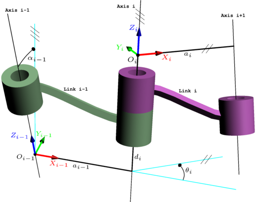 Compared with the classic DH parameters, the coordinates of frame
  is put on axis i-1, not the axis i in classic DH convention. The coordinates of
  is put on the axis i, not the axis i+1 in classic DH convention.
Another difference is that according to the modified convention, the transform matrix is given by the following order of operations:
 and
and  to indicate the length and twist of link n-1 rather than link n. As a consequence,
  is formed only with parameters using the same subscript.
: offset along previous
: angle about previous
: length of the common normal (aka
, but if using this notation, do not confuse with
). Assuming a revolute joint, this is the radius about previous
: angle about common normal, from old
There is some choice in frame layout as to whether the previous
axis or the next
points along the common normal. The latter system allows branching
chains more efficiently, as multiple frames can all point away from
their common ancestor, but in the alternative layout the ancestor can
only point toward one successor. Thus the commonly used notation places
each down-chain axis collinear with the common normal, yielding the transformation calculations shown below.We can note constraints on the relationships between the axes:
- the
- the
- the origin of joint
completes a right-handed reference frame based on
It is common to separate a screw displacement into the product of a pure translation along a line and a pure rotation about the line, so that
![[X_{i}]=\operatorname {Trans}_{{X_{i}}}(r_{{i,i+1}})\operatorname {Rot}_{{X_{i}}}(\alpha _{{i,i+1}}).](https://wikimedia.org/api/rest_v1/media/math/render/svg/158713cb1ead932df740dd529cebcdd2b963cbc9)

![\operatorname{Trans}_{z_{n - 1}}(d_n)
=
\left[
\begin{array}{ccc|c}
1 & 0 & 0 & 0 \\
0 & 1 & 0 & 0 \\
0 & 0 & 1 & d_n \\
\hline
0 & 0 & 0 & 1
\end{array}
\right]](https://wikimedia.org/api/rest_v1/media/math/render/svg/53384aa30ff82a2b85f6433f9cc439b9fecfa719)
![\operatorname{Rot}_{z_{n - 1}}(\theta_n)
=
\left[
\begin{array}{ccc|c}
\cos\theta_n & -\sin\theta_n & 0 & 0 \\
\sin\theta_n & \cos\theta_n & 0 & 0 \\
0 & 0 & 1 & 0 \\
\hline
0 & 0 & 0 & 1
\end{array}
\right]](https://wikimedia.org/api/rest_v1/media/math/render/svg/8f6829532da2c9b95b7838686240621a281d066b)
![\operatorname{Trans}_{x_n}(r_n)
=
\left[
\begin{array}{ccc|c}
1 & 0 & 0 & r_n \\
0 & 1 & 0 & 0 \\
0 & 0 & 1 & 0 \\
\hline
0 & 0 & 0 & 1
\end{array}
\right]](https://wikimedia.org/api/rest_v1/media/math/render/svg/32b9c367824bbe1639372c2a4805c99efd967a5f)
![\operatorname{Rot}_{x_n}(\alpha_n)
=
\left[
\begin{array}{ccc|c}
1 & 0 & 0 & 0 \\
0 & \cos\alpha_n & -\sin\alpha_n & 0 \\
0 & \sin\alpha_n & \cos\alpha_n & 0 \\
\hline
0 & 0 & 0 & 1
\end{array}
\right]](https://wikimedia.org/api/rest_v1/media/math/render/svg/6323ca441a702b252b2d8521dde3ae9c1aa6b662)
![\operatorname{}^{n - 1}T_n
=
\left[
\begin{array}{ccc|c}
\cos\theta_n & -\sin\theta_n \cos\alpha_n & \sin\theta_n \sin\alpha_n & r_n \cos\theta_n \\
\sin\theta_n & \cos\theta_n \cos\alpha_n & -\cos\theta_n \sin\alpha_n & r_n \sin\theta_n \\
0 & \sin\alpha_n & \cos\alpha_n & d_n \\
\hline
0 & 0 & 0 & 1
\end{array}
\right]
=
\left[
\begin{array}{ccc|c}
& & & \\
& R & & T \\
& & & \\
\hline
0 & 0 & 0 & 1
\end{array}
\right]](https://wikimedia.org/api/rest_v1/media/math/render/svg/6963d0c47a3a894ff0719c8df348d188b996074e)
The Denavit and Hartenberg notation gives a standard methodology to write the kinematic equations of a manipulator. This is specially useful for serial manipulators where a matrix is used to represent the pose (position and orientation) of one body with respect to another.
The position of body
with respect to may be represented by a position matrix indicated with the symbol or  to
to ![P_{(n-1)} = M_{n-1,n} P_{(n)} = \left[ \begin{array}{c} x_{n-1} \\y_{n-1} \\z_{n-1} \\ 1 \end{array} \right] = \left[ \begin{array}{ccc|c} X_x & Y_x & Z_x & T_x \\ X_y & Y_y & Z_y & T_y \\ X_z & Y_z & Z_z & T_z \\
\hline
0 & 0 & 0 & 1 \end{array}\right]
\left[ \begin{array}{c} x_{n} \\y_{n} \\z_{n} \\ 1 \end{array} \right]](https://wikimedia.org/api/rest_v1/media/math/render/svg/74ec004742a5c86c744c4073b9d4d6299e7cc46a) submatrix of represents the relative orientation of the two bodies, and the upper right represents their relative position.
submatrix of represents the relative orientation of the two bodies, and the upper right represents their relative position.The position of body
with respect to body can be obtained as the product of the matrices representing the pose of with respect of and that of with respect of 
![M^{-1} =
\left[
\begin{array}{ccc|c}
& & & \\
& R^T & & -R^T T \\
& & & \\
\hline
0 & 0 & 0 & 1
\end{array}
\right]](https://wikimedia.org/api/rest_v1/media/math/render/svg/882df2d7cbe95a1b08c0fc516b7e2d247cf5f84d) is both the transpose and the inverse of the orthogonal matrix , i.e. .
is both the transpose and the inverse of the orthogonal matrix , i.e. .Kinematics
Further matrices can be defined to represent velocity and acceleration of bodies. The velocity of body with respect to body can be represented in frame by the matrix![W_{i,j(k)}=\left[ \begin{array}{ccc|c} 0 & -\omega_z & \omega_y & v_x \\ \omega_z & 0 & -\omega_x & v_y \\ -\omega_y & \omega_x & 0 & v_z \\
\hline
0 & 0 & 0 & 0 \end{array}\right]](https://wikimedia.org/api/rest_v1/media/math/render/svg/e502f568baa4e4d91f1733ea1f5f2ec0d0d41b42) is the angular velocity of body with respect to body and all the components are expressed in frame ; is the velocity of one point of body with respect to body (the pole). The pole is the point of passing through the origin of frame .
is the angular velocity of body with respect to body and all the components are expressed in frame ; is the velocity of one point of body with respect to body (the pole). The pole is the point of passing through the origin of frame .The acceleration matrix can be defined as the sum of the time derivative of the velocity plus the velocity squared
 of a point of body can be evaluated as


The components of velocity and acceleration matrices are expressed in an arbitrary frame
and transform from one frame to another by the following rule

Dynamics
For the dynamics 3 further matrices are necessary to describe the inertia, the linear and angular momentum , and the forces and torques applied to a body.Inertia
:![{\displaystyle J=\left[{\begin{array}{ccc|c}I_{xx}&I_{xy}&I_{xz}&x_{g}m\\I_{yx}&I_{yy}&I_{yz}&y_{g}m\\I_{xz}&I_{yz}&I_{zz}&z_{g}m\\\hline x_{g}m&y_{g}m&z_{g}m&m\end{array}}\right]}](https://wikimedia.org/api/rest_v1/media/math/render/svg/fe721dcdc83f4b02cf7b2b8af820197f125cabc6) is the mass, represent the position of the center of mass, and the terms represent inertia and are defined as
is the mass, represent the position of the center of mass, and the terms represent inertia and are defined as


 , containing force and torque :
![\Phi =\left[{\begin{array}{ccc|c}0&-t_{z}&t_{y}&f_{x}\\t_{z}&0&-t_{x}&f_{y}\\-t_{y}&t_{x}&0&f_{z}\\\hline -f_{x}&-f_{y}&-f_{z}&0\end{array}}\right]](https://wikimedia.org/api/rest_v1/media/math/render/svg/4368085c58c6e9ab64b78ecbb7cca5e33b54f820) , containing linear and angular momentum
, containing linear and angular momentum![\Gamma = \left[ \begin{array}{ccc|c} 0 & -\gamma_z & \gamma_y & \rho_x \\ \gamma_z & 0 & -\gamma_x & \rho_y \\ -\gamma_y & \gamma_x & 0 & \rho_z \\
\hline
-\rho_x & -\rho_y & -\rho_z & 0 \end{array}\right]](https://wikimedia.org/api/rest_v1/media/math/render/svg/73128fb4771872bdccff6c51dc5af41a17610bff) . Transformation of the components from frame to frame follows to rule
. Transformation of the components from frame to frame follows to rule


Newton's law:

 (force equal mass times acceleration) plus
(angular acceleration in function of inertia and angular velocity); the
second equation permits the evaluation of the linear and angular
momentum when velocity and inertia are known.
(force equal mass times acceleration) plus
(angular acceleration in function of inertia and angular velocity); the
second equation permits the evaluation of the linear and angular
momentum when velocity and inertia are known.Modified DH parameters
Some books such as use modified DH parameters. The difference between the classic DH parameters and the modified DH parameters are the locations of the coordinates system attachment to the links and the order of the performed transformations.
Modified DH parameters
is put on axis i-1, not the axis i in classic DH convention. The coordinates of is put on the axis i, not the axis i+1 in classic DH convention.Another difference is that according to the modified convention, the transform matrix is given by the following order of operations:

![\operatorname{}^{n - 1}T_n
=
\left[
\begin{array}{ccc|c}
\cos\theta_n & -\sin\theta_n & 0 & a_{n-1} \\
\sin\theta_n \cos\alpha_{n-1} & \cos\theta_n \cos\alpha_{n-1} & -\sin\alpha_{n-1} & -d_n \sin\alpha_{n-1} \\
\sin\theta_n\sin\alpha_{n-1} & \cos\theta_n \sin\alpha_{n-1} & \cos\alpha_{n-1} & d_n \cos\alpha_{n-1} \\
\hline
0 & 0 & 0 & 1
\end{array}
\right]](https://wikimedia.org/api/rest_v1/media/math/render/svg/c871f4e80e3c6be1cebb018cfb71de2f12e9e340) and to indicate the length and twist of link n-1 rather than link n. As a consequence, is formed only with parameters using the same subscript.
and to indicate the length and twist of link n-1 rather than link n. As a consequence, is formed only with parameters using the same subscript. Robot Inverse Kinematics
|
|
We've seen the forward kinematics problem. The inverse kinematics
problem is much more interesting and its solution is more useful.
At the position level, the problem is stated as, "Given the
desired position of the robot's hand, what must be the angles at all
of the robots joints?" Humans solve this problem all the time without even thinking about it. When you are eating your cereal in the morning you just reach out and grab your spoon. You don't think, "my shoulder needs to do this, my elbow needs to do that, etc." Below we will look at how most robots have to solve the problem. We will start with a very simple example.
The figure above is a schematic of a simple
robot lying in the X-Y plane. The robot has one link of length l
and one joint with angle Ø. The position of the robot's
hand is Xhand. The inverse kinematics problem (at
the position level) for this robot is as follows: Given Xhand
what is the joint angle Ø? We'll start the solution to this
problem by writing down the forward position equation, and
then solve for Ø.
| |||||||||||||||||||||||||||||||||||||||||||||||||||||||||||||||||||||||||||||||||||||||||||||||||||||||