rene decartes in work logic when integrating differntial and integral nodes based on the concept of plotting of laplace dots on the decreasing of both audio and video signal functions within the instrumentation and control systems derived in multi-dimensional moving signals. rene decartes has the principle that a point can move in a multi-dimensional space; the work of rene decartes is continued by Newton where all the points in multi-dimensional space always have an action and reaction force; Newton assumes in the logic of the work of making the formulas that all the dotted objects like the moon always have action and reaction with the nearest star and earth garden then when Einstein gives the logic of his work while continuing the creations of the formula from Newton and rene decartes says that the tick point like the moon always remains when experiencing the action and reaction force of the nearest star unless we meet with a glimmer of light that simultaneously moves with the nearest star when Einstein explains his formula on 4G in G to 4 there is a weak point actually because the weak point is in the conjuntion space adjacent to the multi dimensional on earth for that we need the amplifier of the nearest star and the bright multi-dimensional light rays that move simultaneously toward the nearest point in the multi-dimensional conjuntion space on earth.
XXX . XXX Calculus
Calculus is the mathematical study of continuous change, in the same way that geometry is the study of shape and algebra is the study of generalizations of arithmetic operations. It has two major branches, differential calculus (concerning rates of change and slopes of curves), and integral calculus (concerning accumulation of quantities and the areas under and between curves). These two branches are related to each other by the fundamental theorem of calculus. Both branches make use of the fundamental notions of convergence of infinite sequences and infinite series to a well-defined limit. Generally, modern calculus is considered to have been developed in the 17 th century by Isaac Newton and Gottfried Wilhelm Leibniz. Today, calculus has widespread uses in science, engineering, and economics.
Calculus is a part of modern mathematics education. A course in calculus is a gateway to other, more advanced courses in mathematics devoted to the study of functions and limits, broadly called mathematical analysis. Calculus has historically been called "the calculus of infinitesimals", or "infinitesimal calculus". The term calculus (plural calculi) is also used for naming specific methods of calculation or notation as well as some theories, such as propositional calculus, Ricci calculus, calculus of variations, lambda calculus, and process calculus.
Modern calculus was developed in 17th-century Europe by Isaac Newton and Gottfried Wilhelm Leibniz (independently of each other, first publishing around the same time) but elements of it have appeared in ancient Greece, then in China and the Middle East, and still later again in medieval Europe and in India.

Ancient
The ancient period introduced some of the ideas that led to integral calculus, but does not seem to have developed these ideas in a rigorous and systematic way. Calculations of volume and area, one goal of integral calculus, can be found in the Egyptian Moscow papyrus (13th dynasty,c. 1820 BC), but the formulas are simple instructions, with no indication as to method, and some of them lack major components.[5] From the age ofGreek mathematics, Eudoxus (c. 408–355 BC) used the method of exhaustion, which foreshadows the concept of the limit, to calculate areas and volumes, while Archimedes (c. 287–212 BC) developed this idea further, inventing heuristics which resemble the methods of integral calculus.[6] Themethod of exhaustion was later discovered independently in China by Liu Hui in the 3rd century AD in order to find the area of a circle.[7] In the 5th century AD, Zu Gengzhi, son of Zu Chongzhi, established a method[8][9] that would later be called Cavalieri's principle to find the volume of a sphere.
In the Middle East, Alhazen (c. 965 – c. 1040 ce) derived a formula for the sum of fourth powers. He used the results to carry out what would now be called an integration of this function, where the formulae for the sums of integral squares and fourth powers allowed him to calculate the volume of aparaboloid.[10] In the 14th century, Indian mathematicians gave a non-rigorous method, resembling differentiation, applicable to some trigonometric functions. Madhava of Sangamagrama and the Kerala School of Astronomy and Mathematics thereby stated components of calculus. A complete theory encompassing these components is now well-known in the Western world as the Taylor series or infinite series approximations.[11] However, they were not able to "combine many differing ideas under the two unifying themes of the derivative and the integral, show the connection between the two, and turn calculus into the great problem-solving tool we have today".Medieval
"The calculus was the first achievement of modern mathematics and it is difficult to overestimate its importance. I think it defines more unequivocally than anything else the inception of modern mathematics, and the system of mathematical analysis, which is its logical development, still constitutes the greatest technical advance in exact thinking."Modern
In Europe, the foundational work was a treatise due to Bonaventura Cavalieri, who argued that volumes and areas should be computed as the sums of the volumes and areas of infinitesimally thin cross-sections. The ideas were similar to Archimedes' in The Method, but this treatise is believed to have been lost in the 13th century, and was only rediscovered in the early 20th century, and so would have been unknown to Cavalieri. Cavalieri's work was not well respected since his methods could lead to erroneous results, and the infinitesimal quantities he introduced were disreputable at first.
The formal study of calculus brought together Cavalieri's infinitesimals with the calculus of finite differencesdeveloped in Europe at around the same time. Pierre de Fermat, claiming that he borrowed from Diophantus, introduced the concept of adequality, which represented equality up to an infinitesimal error term.[13] The combination was achieved by John Wallis, Isaac Barrow, and James Gregory, the latter two proving the second fundamental theorem of calculus around 1670.

The product rule and chain rule,[14] the notions of higher derivatives and Taylor series, and of analytic functions were introduced by Isaac Newton in an idiosyncratic notation which he used to solve problems of mathematical physics. In his works, Newton rephrased his ideas to suit the mathematical idiom of the time, replacing calculations with infinitesimals by equivalent geometrical arguments which were considered beyond reproach. He used the methods of calculus to solve the problem of planetary motion, the shape of the surface of a rotating fluid, the oblateness of the earth, the motion of a weight sliding on a cycloid, and many other problems discussed in his Principia Mathematica (1687). In other work, he developed series expansions for functions, including fractional and irrational powers, and it was clear that he understood the principles of the Taylor series. He did not publish all these discoveries, and at this time infinitesimal methods were still considered disreputable.

These ideas were arranged into a true calculus of infinitesimals by Gottfried Wilhelm Leibniz, who was originally accused of plagiarism by Newton.[16] He is now regarded as an independent inventor of and contributor to calculus. His contribution was to provide a clear set of rules for working with infinitesimal quantities, allowing the computation of second and higher derivatives, and providing the product rule andchain rule, in their differential and integral forms. Unlike Newton, Leibniz paid a lot of attention to the formalism, often spending days determining appropriate symbols for concepts.
Today, Leibniz and Newton are usually both given credit for independently inventing and developing calculus. Newton was the first to apply calculus to general physics and Leibniz developed much of the notation used in calculus today. The basic insights that both Newton and Leibniz provided were the laws of differentiation and integration, second and higher derivatives, and the notion of an approximating polynomial series. By Newton's time, the fundamental theorem of calculus was known.
When Newton and Leibniz first published their results, there was great controversy over which mathematician (and therefore which country) deserved credit. Newton derived his results first (later to be published in his Method of Fluxions), but Leibniz published his "Nova Methodus pro Maximis et Minimis" first. Newton claimed Leibniz stole ideas from his unpublished notes, which Newton had shared with a few members of the Royal Society. This controversy divided English-speaking mathematicians from continental European mathematicians for many years, to the detriment of English mathematics. A careful examination of the papers of Leibniz and Newton shows that they arrived at their results independently, with Leibniz starting first with integration and Newton with differentiation. It is Leibniz, however, who gave the new discipline its name. Newton called his calculus "the science of fluxions".
Since the time of Leibniz and Newton, many mathematicians have contributed to the continuing development of calculus. One of the first and most complete works on both infinitesimal and integral calculus was written in 1748 by Maria Gaetana Agnesi.[17][18]

Foundations
Several mathematicians, including Maclaurin, tried to prove the soundness of using infinitesimals, but it would not be until 150 years later when, due to the work of Cauchy and Weierstrass, a way was finally found to avoid mere "notions" of infinitely small quantities.[19] The foundations of differential and integral calculus had been laid. In Cauchy's Cours d'Analyse, we find a broad range of foundational approaches, including a definition of continuity in terms of infinitesimals, and a (somewhat imprecise) prototype of an (ε, δ)-definition of limit in the definition of differentiation.[20] In his work Weierstrass formalized the concept of limit and eliminated infinitesimals (although his definition can actually validate nilsquare infinitesimals). Following the work of Weierstrass, it eventually became common to base calculus on limits instead of infinitesimal quantities, though the subject is still occasionally called "infinitesimal calculus".Bernhard Riemann used these ideas to give a precise definition of the integral. It was also during this period that the ideas of calculus were generalized to Euclidean space and the complex plane.
In modern mathematics, the foundations of calculus are included in the field of real analysis, which contains full definitions and proofs of the theorems of calculus. The reach of calculus has also been greatly extended. Henri Lebesgue invented measure theory and used it to define integrals of all but the most pathological functions. Laurent Schwartzintroduced distributions, which can be used to take the derivative of any function whatsoever.
Limits are not the only rigorous approach to the foundation of calculus. Another way is to use Abraham Robinson's non-standard analysis. Robinson's approach, developed in the 1960s, uses technical machinery from mathematical logic to augment the real number system with infinitesimal and infinite numbers, as in the original Newton-Leibniz conception. The resulting numbers are called hyperreal numbers, and they can be used to give a Leibniz-like development of the usual rules of calculus. There is also smooth infinitesimal analysis, which differs from non-standard analysis in that it mandates neglecting higher power infinitesimals during derivations.
While many of the ideas of calculus had been developed earlier in Greece, China, India, Iraq, Persia, and Japan, the use of calculus began in Europe, during the 17th century, when Isaac Newton and Gottfried Wilhelm Leibniz built on the work of earlier mathematicians to introduce its basic principles. The development of calculus was built on earlier concepts of instantaneous motion and area underneath curves.Significance
Applications of differential calculus include computations involving velocity and acceleration, the slope of a curve, and optimization. Applications of integral calculus include computations involving area, volume, arc length, center of mass, work, and pressure. More advanced applications include power series and Fourier series.
Calculus is also used to gain a more precise understanding of the nature of space, time, and motion. For centuries, mathematicians and philosophers wrestled with paradoxes involving division by zero or sums of infinitely many numbers. These questions arise in the study of motion and area. The ancient Greek philosopher Zeno of Elea gave several famous examples of such paradoxes. Calculus provides tools, especially the limit and the infinite series, that resolve the paradoxes.
Limits and infinitesimalsPrinciples
Calculus is usually developed by working with very small quantities. Historically, the first method of doing so was by infinitesimals. These are objects which can be treated like real numbers but which are, in some sense, "infinitely small". For example, an infinitesimal number could be greater than 0, but less than any number in the sequence 1, 1/2, 1/3, ... and thus less than any positive real number. From this point of view, calculus is a collection of techniques for manipulating infinitesimals. The symbols dx and dy were taken to be infinitesimal, and the derivative was simply their ratio.

The infinitesimal approach fell out of favor in the 19th century because it was difficult to make the notion of an infinitesimal precise. However, the concept was revived in the 20th century with the introduction of non-standard analysis and smooth infinitesimal analysis, which provided solid foundations for the manipulation of infinitesimals.
In the 19th century, infinitesimals were replaced by the epsilon, delta approach to limits. Limits describe the value of a function at a certain input in terms of its values at a nearby input. They capture small-scale behavior in the context of the real number system. In this treatment, calculus is a collection of techniques for manipulating certain limits. Infinitesimals get replaced by very small numbers, and the infinitely small behavior of the function is found by taking the limiting behavior for smaller and smaller numbers. Limits were the first way to provide rigorous foundations for calculus, and for this reason they are the standard approach.
Differential calculus

Differential calculus is the study of the definition, properties, and applications of the derivative of a function. The process of finding the derivative is called differentiation. Given a function and a point in the domain, the derivative at that point is a way of encoding the small-scale behavior of the function near that point. By finding the derivative of a function at every point in its domain, it is possible to produce a new function, called the derivative function or just the derivative of the original function. In formal terms, the derivative is a linear operator which takes a function as its input and produces a second function as its output. This is more abstract than many of the processes studied in elementary algebra, where functions usually input a number and output another number. For example, if the doubling function is given the input three, then it outputs six, and if the squaring function is given the input three, then it outputs nine. The derivative, however, can take the squaring function as an input. This means that the derivative takes all the information of the squaring function—such as that two is sent to four, three is sent to nine, four is sent to sixteen, and so on—and uses this information to produce another function. The function produced by deriving the squaring function turns out to be the doubling function.
In more explicit terms the "doubling function" may be denoted by g(x) = 2x and the "squaring function" by f(x) = x2. The "derivative" now takes the function f(x), defined by the expression "x2", as an input, that is all the information —such as that two is sent to four, three is sent to nine, four is sent to sixteen, and so on— and uses this information to output another function, the function g(x) = 2x, as will turn out.
The most common symbol for a derivative is an apostrophe-like mark called prime. Thus, the derivative of a function called f is denoted by f′, pronounced "f prime". For instance, iff(x) = x2 is the squaring function, then f′(x) = 2x is its derivative (the doubling function g from above). This notation is known as Lagrange's notation.
If the input of the function represents time, then the derivative represents change with respect to time. For example, if f is a function that takes a time as input and gives the position of a ball at that time as output, then the derivative of f is how the position is changing in time, that is, it is the velocity of the ball.
If a function is linear (that is, if the graph of the function is a straight line), then the function can be written as y = mx + b, where x is the independent variable, y is the dependent variable, b is the y-intercept, and:

This gives an exact value for the slope of a straight line. If the graph of the function is not a straight line, however, then the change in y divided by the change in x varies. Derivatives give an exact meaning to the notion of change in output with respect to change in input. To be concrete, let f be a function, and fix a point a in the domain of f.(a, f(a)) is a point on the graph of the function. If h is a number close to zero, then a + h is a number close to a. Therefore, (a + h, f(a + h)) is close to (a, f(a)). The slope between these two points is

This expression is called a difference quotient. A line through two points on a curve is called a secant line, so m is the slope of the secant line between (a, f(a)) and(a + h, f(a + h)). The secant line is only an approximation to the behavior of the function at the point a because it does not account for what happens between a and a + h. It is not possible to discover the behavior at a by setting h to zero because this would require dividing by zero, which is undefined. The derivative is defined by taking the limit as htends to zero, meaning that it considers the behavior of f for all small values of h and extracts a consistent value for the case when h equals zero:

Geometrically, the derivative is the slope of the tangent line to the graph of f at a. The tangent line is a limit of secant lines just as the derivative is a limit of difference quotients. For this reason, the derivative is sometimes called the slope of the function f.
Here is a particular example, the derivative of the squaring function at the input 3. Let f(x) = x2 be the squaring function.


The slope of the tangent line to the squaring function at the point (3, 9) is 6, that is to say, it is going up six times as fast as it is going to the right. The limit process just described can be performed for any point in the domain of the squaring function. This defines the derivative function of the squaring function, or just the derivative of the squaring function for short. A computation similar to the one above shows that the derivative of the squaring function is the doubling function.
Leibniz notation
A common notation, introduced by Leibniz, for the derivative in the example above is

In an approach based on limits, the symbol dydx is to be interpreted not as the quotient of two numbers but as a shorthand for the limit computed above. Leibniz, however, did intend it to represent the quotient of two infinitesimally small numbers, dy being the infinitesimally small change in y caused by an infinitesimally small change dx applied to x. We can also think of ddx as a differentiation operator, which takes a function as an input and gives another function, the derivative, as the output. For example:

In this usage, the dx in the denominator is read as "with respect to x". Even when calculus is developed using limits rather than infinitesimals, it is common to manipulate symbols like dx and dy as if they were real numbers; although it is possible to avoid such manipulations, they are sometimes notationally convenient in expressing operations such as the total derivative.
Integral calculus
Integral calculus is the study of the definitions, properties, and applications of two related concepts, the indefinite integral and the definite integral. The process of finding the value of an integral is called integration. In technical language, integral calculus studies two related linear operators.
The indefinite integral, also known as the antiderivative, is the inverse operation to the derivative. F is an indefinite integral of f when f is a derivative of F. (This use of lower- and upper-case letters for a function and its indefinite integral is common in calculus.)
The definite integral inputs a function and outputs a number, which gives the algebraic sum of areas between the graph of the input and the x-axis. The technical definition of the definite integral involves the limit of a sum of areas of rectangles, called a Riemann sum.
A motivating example is the distances traveled in a given time.

If the speed is constant, only multiplication is needed, but if the speed changes, a more powerful method of finding the distance is necessary. One such method is to approximate the distance traveled by breaking up the time into many short intervals of time, then multiplying the time elapsed in each interval by one of the speeds in that interval, and then taking the sum (a Riemann sum) of the approximate distance traveled in each interval. The basic idea is that if only a short time elapses, then the speed will stay more or less the same. However, a Riemann sum only gives an approximation of the distance traveled. We must take the limit of all such Riemann sums to find the exact distance traveled.


When velocity is constant, the total distance traveled over the given time interval can be computed by multiplying velocity and time. For example, travelling a steady 50 mph for 3 hours results in a total distance of 150 miles. In the diagram on the left, when constant velocity and time are graphed, these two values form a rectangle with height equal to the velocity and width equal to the time elapsed. Therefore, the product of velocity and time also calculates the rectangular area under the (constant) velocity curve. This connection between the area under a curve and distance traveled can be extended to any irregularly shaped region exhibiting a fluctuating velocity over a given time period. If f(x) in the diagram on the right represents speed as it varies over time, the distance traveled (between the times represented by a and b) is the area of the shaded region s.
To approximate that area, an intuitive method would be to divide up the distance between a and b into a number of equal segments, the length of each segment represented by the symbol Δx. For each small segment, we can choose one value of the function f(x). Call that value h. Then the area of the rectangle with base Δx and height h gives the distance (time Δx multiplied by speed h) traveled in that segment. Associated with each segment is the average value of the function above it, f(x) = h. The sum of all such rectangles gives an approximation of the area between the axis and the curve, which is an approximation of the total distance traveled. A smaller value for Δx will give more rectangles and in most cases a better approximation, but for an exact answer we need to take a limit as Δx approaches zero.
The symbol of integration is , an elongated S (the S stands for "sum"). The definite integral is written as:


and is read "the integral from a to b of f-of-x with respect to x." The Leibniz notation dx is intended to suggest dividing the area under the curve into an infinite number of rectangles, so that their width Δx becomes the infinitesimally small dx. In a formulation of the calculus based on limits, the notation

is to be understood as an operator that takes a function as an input and gives a number, the area, as an output. The terminating differential, dx, is not a number, and is not being multiplied by f(x), although, serving as a reminder of the Δx limit definition, it can be treated as such in symbolic manipulations of the integral. Formally, the differential indicates the variable over which the function is integrated and serves as a closing bracket for the integration operator.
The indefinite integral, or antiderivative, is written:

Functions differing by only a constant have the same derivative, and it can be shown that the antiderivative of a given function is actually a family of functions differing only by a constant. Since the derivative of the function y = x2 + C, where C is any constant, is y′ = 2x, the antiderivative of the latter given by:

The unspecified constant C present in the indefinite integral or antiderivative is known as the constant of integration.
Fundamental theorem
The fundamental theorem of calculus states that differentiation and integration are inverse operations. More precisely, it relates the values of antiderivatives to definite integrals. Because it is usually easier to compute an antiderivative than to apply the definition of a definite integral, the fundamental theorem of calculus provides a practical way of computing definite integrals. It can also be interpreted as a precise statement of the fact that differentiation is the inverse of integration.
The fundamental theorem of calculus states: If a function f is continuous on the interval [a, b] and if F is a function whose derivative is f on the interval (a, b), then

Furthermore, for every x in the interval (a, b),

This realization, made by both Newton and Leibniz, who based their results on earlier work by Isaac Barrow, was key to the proliferation of analytic results after their work became known. The fundamental theorem provides an algebraic method of computing many definite integrals—without performing limit processes—by finding formulas for antiderivatives. It is also a prototype solution of a differential equation. Differential equations relate an unknown function to its derivatives, and are ubiquitous in the sciences.

Applications
Calculus is used in every branch of the physical sciences, actuarial science, computer science, statistics, engineering, economics, business, medicine, demography, and in other fields wherever a problem can be mathematically modeled and an optimal solution is desired. It allows one to go from (non-constant) rates of change to the total change or vice versa, and many times in studying a problem we know one and are trying to find the other.
Physics makes particular use of calculus; all concepts in classical mechanics and electromagnetism are related through calculus. The massof an object of known density, the moment of inertia of objects, as well as the total energy of an object within a conservative field can be found by the use of calculus. An example of the use of calculus in mechanics is Newton's second law of motion: historically stated it expressly uses the term "change of motion" which implies the derivative saying The change of momentum of a body is equal to the resultant force acting on the body and is in the same direction. Commonly expressed today as Force = Mass × acceleration, it implies differential calculus because acceleration is the time derivative of velocity or second time derivative of trajectory or spatial position. Starting from knowing how an object is accelerating, we use calculus to derive its path.
Maxwell's theory of electromagnetism and Einstein's theory of general relativity are also expressed in the language of differential calculus. Chemistry also uses calculus in determining reaction rates and radioactive decay. In biology, population dynamics starts with reproduction and death rates to model population changes.
Calculus can be used in conjunction with other mathematical disciplines. For example, it can be used with linear algebra to find the "best fit" linear approximation for a set of points in a domain. Or it can be used in probability theory to determine the probability of a continuous random variable from an assumed density function. In analytic geometry, the study of graphs of functions, calculus is used to find high points and low points (maxima and minima), slope, concavity and inflection points.
Green's Theorem, which gives the relationship between a line integral around a simple closed curve C and a double integral over the plane region D bounded by C, is applied in an instrument known as a planimeter, which is used to calculate the area of a flat surface on a drawing. For example, it can be used to calculate the amount of area taken up by an irregularly shaped flower bed or swimming pool when designing the layout of a piece of property.
Discrete Green's Theorem, which gives the relationship between a double integral of a function around a simple closed rectangular curve C and a linear combination of the antiderivative's values at corner points along the edge of the curve, allows fast calculation of sums of values in rectangular domains. For example, it can be used to efficiently calculate sums of rectangular domains in images, in order to rapidly extract features and detect object; another algorithm that could be used is the summed area table.
In the realm of medicine, calculus can be used to find the optimal branching angle of a blood vessel so as to maximize flow. From the decay laws for a particular drug's elimination from the body, it is used to derive dosing laws. In nuclear medicine, it is used to build models of radiation transport in targeted tumor therapies.
In economics, calculus allows for the determination of maximal profit by providing a way to easily calculate both marginal cost and marginal revenue.
Calculus is also used to find approximate solutions to equations; in practice it is the standard way to solve differential equations and do root finding in most applications. Examples are methods such as Newton's method, fixed point iteration, and linear approximation. For instance, spacecraft use a variation of the Euler method to approximate curved courses within zero gravity environments.
Over the years, many reformulations of calculus have been investigated for different purposes.Varieties
Non-standard calculus
Imprecise calculations with infinitesimals were widely replaced with the rigorous (ε, δ)-definition of limit starting in the 1870s. Meanwhile, calculations with infinitesimals persisted and often led to correct results. This led Abraham Robinson to investigate if it were possible to develop a number system with infinitesimal quantities over which the theorems of calculus were still valid. In 1960, building upon the work of Edwin Hewitt and Jerzy Łoś, he succeeded in developing non-standard analysis. The theory of non-standard analysis is rich enough to be applied in many branches of mathematics. As such, books and articles dedicated solely to the traditional theorems of calculus often go by the title non-standard calculus.
Smooth infinitesimal analysis
This is another reformulation of the calculus in terms of infinitesimals. Based on the ideas of F. W. Lawvere and employing the methods of category theory, it views all functions as being continuous and incapable of being expressed in terms of discrete entities. One aspect of this formulation is that the law of excluded middle does not hold in this formulation.
Constructive analysis
Constructive mathematics is a branch of mathematics that insists that proofs of the existence of a number, function, or other mathematical object should give a construction of the object. As such constructive mathematics also rejects the law of excluded middle. Reformulations of calculus in a constructive framework are generally part of the subject ofconstructive analysis.
XXX . XXX 4% zero Fourier series
In mathematics, a Fourier series (English: /ˈfʊəriˌeɪ/)[1] is a way to represent a function as the sum of simple sine waves. More formally, it decomposes any periodic function or periodic signal into the sum of a (possibly infinite) set of simple oscillating functions, namely sines and cosines (or, equivalently, complex exponentials). The discrete-time Fourier transform is a periodic function, often defined in terms of a Fourier series. The Z-transform, another example of application, reduces to a Fourier series for the important case |z|=1. Fourier series are also central to the original proof of the Nyquist–Shannon sampling theorem. The study of Fourier series is a branch of Fourier analysis.
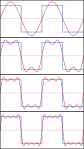
 The first four partial sums of the Fourier series for a square wave
The Fourier series is named in honour of Jean-Baptiste Joseph Fourier (1768–1830), who made important contributions to the study of trigonometric series, after preliminary investigations by Leonhard Euler, Jean le Rond d'Alembert, and Daniel Bernoulli.[nb 1] Fourier introduced the series for the purpose of solving the heat equation in a metal plate, publishing his initial results in his 1807 Mémoire sur la propagation de la chaleur dans les corps solides (Treatise on the propagation of heat in solid bodies), and publishing hisThéorie analytique de la chaleur (Analytical theory of heat) in 1822. The Mémoire introduced Fourier analysis, specifically Fourier series. Through Fourier's research the fact was established that an arbitrary (continuous)[2] function can be represented by a trigonometric series. The first announcement of this great discovery was made by Fourier in 1807, before the French Academy.[3] Early ideas of decomposing a periodic function into the sum of simple oscillating functions date back to the 3rd century BC, when ancient astronomers proposed an empiric model of planetary motions, based on deferents and epicycles.
The heat equation is a partial differential equation. Prior to Fourier's work, no solution to the heat equation was known in the general case, although particular solutions were known if the heat source behaved in a simple way, in particular, if the heat source was a sine or cosine wave. These simple solutions are now sometimes called eigensolutions. Fourier's idea was to model a complicated heat source as a superposition (or linear combination) of simple sine and cosine waves, and to write the solution as a superposition of the corresponding eigensolutions. This superposition or linear combination is called the Fourier series.
From a modern point of view, Fourier's results are somewhat informal, due to the lack of a precise notion of function and integral in the early nineteenth century. Later, Peter Gustav Lejeune Dirichlet[4] and Bernhard Riemann[5][6][7] expressed Fourier's results with greater precision and formality.
Although the original motivation was to solve the heat equation, it later became obvious that the same techniques could be applied to a wide array of mathematical and physical problems, and especially those involving linear differential equations with constant coefficients, for which the eigensolutions are sinusoids. The Fourier series has many such applications in electrical engineering, vibration analysis, acoustics, optics, signal processing, image processing, quantum mechanics, econometrics,[8] thin-walled shell theory,[9]etc.
In this section, s(x) denotes a function of the real variable x, and s is integrable on an interval [x0, x0 + P], for real numbers x0 and P. We will attempt to represent s in that interval as an infinite sum, or series, of harmonically related sinusoidal functions. Outside the interval, the series is periodic with period P (frequency 1/P). It follows that if s also has that property, the approximation is valid on the entire real line. We can begin with a finite summation (or partial sum):Definition

is a periodic function with period P. Using the identities:


we can also write the function in these equivalent forms:

where:

The inverse relationships between the coefficients are:

When the coefficients (known as Fourier coefficients) are computed as follows:[10]


approximates on and the approximation improves as N → ∞. The infinite sum, is called the Fourier series representation of
Both components of a complex-valued function are real-valued functions that can be represented by a Fourier series. The two sets of coefficients and the partial sum are given by:
![\scriptstyle [x_0,\ x_0+P],](https://wikimedia.org/api/rest_v1/media/math/render/svg/e15dd8a7d5176a8625325e2afb151fbdd825a142)


Complex-valued functions
- and


This is the same formula as before except cn and c−n are no longer complex conjugates. The formula for cn is also unchanged:

Convergence


Example 1: a simple Fourier series

![(-\pi ,\pi ]](https://wikimedia.org/api/rest_v1/media/math/render/svg/7fbb1843079a9df3d3bbcce3249bb2599790de9c)

We now use the formula above to give a Fourier series expansion of a very simple function. Consider a sawtooth wave


In this case, the Fourier coefficients are given by

It can be proven that Fourier series converges to s(x) at every point x where s is differentiable, and therefore:
- (Eq.1)
![\begin{align}
s(x) &= \frac{a_0}{2} + \sum_{n=1}^\infty \left[a_n\cos\left(nx\right)+b_n\sin\left(nx\right)\right] \\
&=\frac{2}{\pi}\sum_{n=1}^\infty \frac{(-1)^{n+1}}{n} \sin(nx), \quad \mathrm{for} \quad x - \pi \notin 2 \pi \mathbf{Z}.
\end{align}](https://wikimedia.org/api/rest_v1/media/math/render/svg/e4f7723030e9a65dde2b59bdffde660c5ac6d1a4)
When x = π, the Fourier series converges to 0, which is the half-sum of the left- and right-limit of s at x = π. This is a particular instance of the Dirichlet theorem for Fourier series.

This example leads us to a solution to the Basel problem.
The Fourier series expansion of our function in Example 1 looks more complicated than the simple formula s(x) = x/π, so it is not immediately apparent why one would need the Fourier series. While there are many applications, Fourier's motivation was in solving theheat equation. For example, consider a metal plate in the shape of a square whose side measures π meters, with coordinates (x, y) ∈ [0, π] × [0, π]. If there is no heat source within the plate, and if three of the four sides are held at 0 degrees Celsius, while the fourth side, given by y = π, is maintained at the temperature gradient T(x, π) = x degrees Celsius, for x in (0, π), then one can show that the stationary heat distribution (or the heat distribution after a long period of time has elapsed) is given byExample 2: Fourier's motivation

Here, sinh is the hyperbolic sine function. This solution of the heat equation is obtained by multiplying each term of Eq.1 by sinh(ny)/sinh(nπ). While our example function s(x) seems to have a needlessly complicated Fourier series, the heat distribution T(x, y) is nontrivial. The function T cannot be written as a closed-form expression. This method of solving the heat problem was made possible by Fourier's work.
Another application of this Fourier series is to solve the Basel problem by using Parseval's theorem. The example generalizes and one may compute ζ(2n), for any positive integer n.Other applications
The notation cn is inadequate for discussing the Fourier coefficients of several different functions. Therefore, it is customarily replaced by a modified form of the function (s, in this case), such as or S, and functional notation often replaces subscripting:
Other common notations
![\begin{align}
s_{\infty}(x) &= \sum_{n=-\infty}^\infty \hat{s}(n)\cdot e^{i\tfrac{2\pi nx}{P}} \\
&= \sum_{n=-\infty}^\infty S[n]\cdot e^{j\tfrac{2\pi nx}{P}} &&\scriptstyle \text{common engineering notation}
\end{align}](https://wikimedia.org/api/rest_v1/media/math/render/svg/1948743e8e50b99560a2e018c78b35e14e2111a1)
In engineering, particularly when the variable x represents time, the coefficient sequence is called a frequency domain representation. Square brackets are often used to emphasize that the domain of this function is a discrete set of frequencies.
Another commonly used frequency domain representation uses the Fourier series coefficients to modulate a Dirac comb:
![S(f) \ \stackrel{\mathrm{def}}{=} \ \sum_{n=-\infty}^\infty S[n]\cdot \delta \left(f-\frac{n}{P}\right),](https://wikimedia.org/api/rest_v1/media/math/render/svg/191fd9d4420479ce5300b692fbc43c0e5e703e89)
where f represents a continuous frequency domain. When variable x has units of seconds, f has units of hertz. The "teeth" of the comb are spaced at multiples (i.e. harmonics) of 1/P, which is called the fundamental frequency. can be recovered from this representation by an inverse Fourier transform:

![\begin{align}
\mathcal{F}^{-1}\{S(f)\} &= \int_{-\infty}^\infty \left( \sum_{n=-\infty}^\infty S[n]\cdot \delta \left(f-\frac{n}{P}\right)\right) e^{i 2 \pi f x}\,df, \\
&= \sum_{n=-\infty}^\infty S[n]\cdot \int_{-\infty}^\infty \delta\left(f-\frac{n}{P}\right) e^{i 2 \pi f x}\,df, \\
&= \sum_{n=-\infty}^\infty S[n]\cdot e^{i\tfrac{2\pi nx}{P}} \ \ \stackrel{\mathrm{def}}{=} \ s_{\infty}(x).
\end{align}](https://wikimedia.org/api/rest_v1/media/math/render/svg/3f87bc7f858006ce49e2b5c40d429076b92b96df)
The constructed function S(f) is therefore commonly referred to as a Fourier transform, even though the Fourier integral of a periodic function is not convergent at the harmonic frequencies.[nb 2]
Beginnings[edit]
| “ |
Multiplying both sides by , and then integrating from to yields:
| ” |
| — Joseph Fourier, Mémoire sur la propagation de la chaleur dans les corps solides. (1807) | ||


This immediately gives any coefficient ak of the trigonometrical series for φ(y) for any function which has such an expansion. It works because if φ has such an expansion, then (under suitable convergence assumptions) the integral

can be carried out term-by-term. But all terms involving for j ≠ k vanish when integrated from −1 to 1, leaving only the kth term.

In these few lines, which are close to the modern formalism used in Fourier series, Fourier revolutionized both mathematics and physics. Although similar trigonometric series were previously used by Euler, d'Alembert, Daniel Bernoulli and Gauss, Fourier believed that such trigonometric series could represent any arbitrary function. In what sense that is actually true is a somewhat subtle issue and the attempts over many years to clarify this idea have led to important discoveries in the theories of convergence, function spaces, and harmonic analysis.
When Fourier submitted a later competition essay in 1811, the committee (which included Lagrange, Laplace, Malus and Legendre, among others) concluded: ...the manner in which the author arrives at these equations is not exempt of difficulties and...his analysis to integrate them still leaves something to be desired on the score of generality and evenrigour .
Since Fourier's time, many different approaches to defining and understanding the concept of Fourier series have been discovered, all of which are consistent with one another, but each of which emphasizes different aspects of the topic. Some of the more powerful and elegant approaches are based on mathematical ideas and tools that were not available at the time Fourier completed his original work. Fourier originally defined the Fourier series for real-valued functions of real arguments, and using the sine and cosine functions as the basis set for the decomposition.Birth of harmonic analysis
Many other Fourier-related transforms have since been defined, extending the initial idea to other applications. This general area of inquiry is now sometimes called harmonic analysis. A Fourier series, however, can be used only for periodic functions, or for functions on a bounded (compact) interval.
Extensions
We can also define the Fourier series for functions of two variables x and y in the square [−π, π] × [−π, π]:


Aside from being useful for solving partial differential equations such as the heat equation, one notable application of Fourier series on the square is in image compression. In particular, the jpeg image compression standard uses the two-dimensional discrete cosine transform, which is a Fourier transform using the cosine basis functions.
The three-dimensional Bravais lattice is defined as the set of vectors of the form:Fourier series of Bravais-lattice-periodic-function

where ni are integers and ai are three linearly independent vectors. Assuming we have some function, f(r), such that it obeys the following condition for any Bravais lattice vectorR: f(r) = f(r + R), we could make a Fourier series of it. This kind of function can be, for example, the effective potential that one electron "feels" inside a periodic crystal. It is useful to make a Fourier series of the potential then when applying Bloch's theorem. First, we may write any arbitrary vector r in the coordinate-system of the lattice:

where ai = |ai|.
Thus we can define a new function,

This new function, , is now a function of three-variables, each of which has periodicity a1, a2, a3 respectively:

- .

If we write a series for g on the interval [0, a1] for x1, we can define the following:

And then we can write:

Further defining:
![\begin{align}
h^\mathrm{two}(m_1, m_2, x_3) & := \frac{1}{a_2}\int_0^{a_2} h^\mathrm{one}(m_1, x_2, x_3)\cdot e^{-i 2\pi \frac{m_2}{a_2} x_2}\, dx_2 \\[12pt]
& = \frac{1}{a_2}\int_0^{a_2} dx_2 \frac{1}{a_1}\int_0^{a_1} dx_1 g(x_1, x_2, x_3)\cdot e^{-i 2\pi \left(\frac{m_1}{a_1} x_1+\frac{m_2}{a_2} x_2\right)}
\end{align}](https://wikimedia.org/api/rest_v1/media/math/render/svg/8b375ad1bad97e4cee6cfa9c82d20582af5ba6b4)
We can write g once again as:

Finally applying the same for the third coordinate, we define:
![\begin{align}
h^\mathrm{three}(m_1, m_2, m_3) & := \frac{1}{a_3}\int_0^{a_3} h^\mathrm{two}(m_1, m_2, x_3)\cdot e^{-i 2\pi \frac{m_3}{a_3} x_3}\, dx_3 \\[12pt]
& = \frac{1}{a_3}\int_0^{a_3} dx_3 \frac{1}{a_2}\int_0^{a_2} dx_2 \frac{1}{a_1}\int_0^{a_1} dx_1 g(x_1, x_2, x_3)\cdot e^{-i 2\pi \left(\frac{m_1}{a_1} x_1+\frac{m_2}{a_2} x_2 + \frac{m_3}{a_3} x_3\right)}
\end{align}](https://wikimedia.org/api/rest_v1/media/math/render/svg/bac3a4c30ff78f3abc70b6b65a6274b8899ca038)
We write g as:

Re-arranging:

Now, every reciprocal lattice vector can be written as , where li are integers and gi are the reciprocal lattice vectors, we can use the fact that to calculate that for any arbitrary reciprocal lattice vector K and arbitrary vector in space r, their scalar product is:


And so it is clear that in our expansion, the sum is actually over reciprocal lattice vectors:

where

Assuming

we can solve this system of three linear equations for x, y, and z in terms of x1, x2 and x3 in order to calculate the volume element in the original cartesian coordinate system. Once we have x, y, and z in terms of x1, x2 and x3, we can calculate the Jacobian determinant:
![{\displaystyle {\begin{vmatrix}{\dfrac {\partial x_{1}}{\partial x}}&{\dfrac {\partial x_{1}}{\partial y}}&{\dfrac {\partial x_{1}}{\partial z}}\\[12pt]{\dfrac {\partial x_{2}}{\partial x}}&{\dfrac {\partial x_{2}}{\partial y}}&{\dfrac {\partial x_{2}}{\partial z}}\\[12pt]{\dfrac {\partial x_{3}}{\partial x}}&{\dfrac {\partial x_{3}}{\partial y}}&{\dfrac {\partial x_{3}}{\partial z}}\end{vmatrix}}}](https://wikimedia.org/api/rest_v1/media/math/render/svg/5e5df9134486606d6a55c8ec4a96ee3ca353e924)
which after some calculation and applying some non-trivial cross-product identities can be shown to be equal to:

(it may be advantageous for the sake of simplifying calculations, to work in such a cartesian coordinate system, in which it just so happens that a1 is parallel to the x axis, a2 lies in the x-y plane, and a3 has components of all three axes). The denominator is exactly the volume of the primitive unit cell which is enclosed by the three primitive-vectors a1, a2 anda3. In particular, we now know that

We can write now h(K) as an integral with the traditional coordinate system over the volume of the primitive cell, instead of with the x1, x2 and x3 variables:

And C is the primitive unit cell, thus, is the volume of the primitive unit cell.

Hilbert space interpretation
In the language of Hilbert spaces, the set of functions is an orthonormal basis for the space L2([−π, π]) of square-integrable functions on [−π, π]. This space is actually a Hilbert space with an inner product given for any two elements f and g by


The basic Fourier series result for Hilbert spaces can be written as


This corresponds exactly to the complex exponential formulation given above. The version with sines and cosines is also justified with the Hilbert space interpretation. Indeed, the sines and cosines form an orthogonal set:


(where δmn is the Kronecker delta), and

furthermore, the sines and cosines are orthogonal to the constant function 1. An orthonormal basis forL2([−π,π]) consisting of real functions is formed by the functions 1 and √2 cos(nx), √2 sin(nx) with n = 1, 2,... The density of their span is a consequence of the Stone–Weierstrass theorem, but follows also from the properties of classical kernels like the Fejér kernel.
We say that f belongs to if f is a 2π-periodic function on R which is k times differentiable, and its kth derivative is continuous.
Properties
- If f is an odd function, then an = 0 for all n.
- If f is an even function, then bn = 0 for all n.
- If f is integrable, , and This result is known as the Riemann–Lebesgue lemma.
- A doubly infinite sequence {an} in c0(Z) is the sequence of Fourier coefficients of a function in L1([0, 2π]) if and only if it is a convolution of two sequences in . See [13]
- If , then the Fourier coefficients of the derivative f′ can be expressed in terms of the Fourier coefficients of the function f, via the formula .
- If , then . In particular, since tends to zero, we have that tends to zero, which means that the Fourier coefficients converge to zero faster than the kth power of n.
- Parseval's theorem. If f belongs to L2([−π, π]), then .
- Plancherel's theorem. If are coefficients and then there is a unique function such that for every n.
- The first convolution theorem states that if f and g are in L1([−π, π]), the Fourier series coefficients of the 2π-periodic convolution of f and g are given by:


![f\in L^2([-\pi,\pi])](https://wikimedia.org/api/rest_v1/media/math/render/svg/74d27747bf5e28fa54e94f218bd9296213ef25c5)

 = 2\pi\cdot \hat{f}(n)\cdot\hat{g}(n),](https://wikimedia.org/api/rest_v1/media/math/render/svg/956ea404aa998519c088c08c9a9e9f29c9bd38f0)
- where:
 \ &\stackrel{\mathrm{def}}{=} \int_{-\pi}^{\pi} f(u)\cdot g[\text{pv}(x-u)] du, &&
\big(\text{and }\underbrace{\text{pv}(x) \ \stackrel{\mathrm{def}}{=} \text{Arg}\left(e^{ix}\right)
}_{\text{principal value}}\big)\\
&= \int_{-\pi}^{\pi} f(u)\cdot g(x-u)\, du, &&\scriptstyle \text{when g(x) is 2}\pi\text{-periodic.}\\
&= \int_{2\pi} f(u)\cdot g(x-u)\, du, &&\scriptstyle \text{when both functions are 2}\pi\text{-periodic, and the integral is over any 2}\pi\text{ interval.}
\end{align}](https://wikimedia.org/api/rest_v1/media/math/render/svg/1223be49e9c8285ec78e1a81ac52e7f983702eeb)
- The second convolution theorem states that the Fourier series coefficients of the product of f and g are given by the discrete convolution of the and sequences:


 = [\hat{f}*\hat{g}](n).](https://wikimedia.org/api/rest_v1/media/math/render/svg/0a01ca431cbe51c2353a325265bb70204e5a1ae1)
Compact groups
One of the interesting properties of the Fourier transform which we have mentioned, is that it carries convolutions to pointwise products. If that is the property which we seek to preserve, one can produce Fourier series on any compact group. Typical examples include those classical groups that are compact. This generalizes the Fourier transform to all spaces of the form L2(G), where G is a compact group, in such a way that the Fourier transform carries convolutions to pointwise products. The Fourier series exists and converges in similar ways to the [−π,π] case.
An alternative extension to compact groups is the Peter–Weyl theorem, which proves results about representations of compact groups analogous to those about finite groups.

Riemannian manifolds
If the domain is not a group, then there is no intrinsically defined convolution. However, if X is a compact Riemannian manifold, it has aLaplace–Beltrami operator. The Laplace–Beltrami operator is the differential operator that corresponds to Laplace operator for the Riemannian manifold X. Then, by analogy, one can consider heat equations on X. Since Fourier arrived at his basis by attempting to solve the heat equation, the natural generalization is to use the eigensolutions of the Laplace–Beltrami operator as a basis. This generalizes Fourier series to spaces of the type L2(X), where X is a Riemannian manifold. The Fourier series converges in ways similar to the [−π, π] case. A typical example is to take X to be the sphere with the usual metric, in which case the Fourier basis consists of spherical harmonics.
Locally compact Abelian groups
The generalization to compact groups discussed above does not generalize to noncompact, nonabelian groups. However, there is a straightforward generalization to Locally Compact Abelian (LCA) groups.
This generalizes the Fourier transform to L1(G) or L2(G), where G is an LCA group. If G is compact, one also obtains a Fourier series, which converges similarly to the [−π, π] case, but if G is noncompact, one obtains instead a Fourier integral. This generalization yields the usual Fourier transform when the underlying locally compact Abelian group is R.
An important question for the theory as well as applications is that of convergence. In particular, it is often necessary in applications to replace the infinite series by a finite one,
Approximation and convergence of Fourier series

This is called a partial sum. We would like to know, in which sense does fN(x) converge to f(x) as N → ∞.
We say that p is a trigonometric polynomial of degree N when it is of the formLeast squares property

Note that fN is a trigonometric polynomial of degree N. Parseval's theorem implies that


Convergence
Because of the least squares property, and because of the completeness of the Fourier basis, we obtain an elementary convergence result.
Theorem. If f belongs to L2([−π, π]), then f∞ converges to f in L2([−π, π]), that is, converges to 0 as N → ∞.

We have already mentioned that if f is continuously differentiable, then is the nth Fourier coefficient of the derivative f′. It follows, essentially from the Cauchy–Schwarz inequality, that f∞ is absolutely summable. The sum of this series is a continuous function, equal to f, since the Fourier series converges in the mean to f:

This result can be proven easily if f is further assumed to be C2, since in that case tends to zero as n → ∞. More generally, the Fourier series is absolutely summable, thus converges uniformly to f, provided that f satisfies a Hölder condition of order α > ½. In the absolutely summable case, the inequality proves uniform convergence.


Many other results concerning the convergence of Fourier series are known, ranging from the moderately simple result that the series converges at x if f is differentiable at x, toLennart Carleson's much more sophisticated result that the Fourier series of an L2 function actually converges almost everywhere.
These theorems, and informal variations of them that don't specify the convergence conditions, are sometimes referred to generically as "Fourier's theorem" or "the Fourier theorem".
Since Fourier series have such good convergence properties, many are often surprised by some of the negative results. For example, the Fourier series of a continuous T-periodic function need not converge pointwise. The uniform boundedness principle yields a simple non-constructive proof of this fact.Divergence
In 1922, Andrey Kolmogorov published an article titled "Une série de Fourier-Lebesgue divergente presque partout" in which he gave an example of a Lebesgue-integrable function whose Fourier series diverges almost everywhere. He later constructed an example of an integrable function whose Fourier series diverges everywhere (Katznelson 1976).
ATS theoremSee
- Dirichlet kernel
- Discrete Fourier transform
- Fast Fourier transform
- Fejér's theorem
- Fourier analysis
- Fourier sine and cosine series
- Fourier transform
- Gibbs phenomenon
- Laurent series – the substitution q = eix transforms a Fourier series into a Laurent series, or conversely. This is used in the q-series expansion of the j-invariant.
- Multidimensional transform
- Spectral theory
- Sturm–Liouville theory
Notes
- ^ Since the integral defining the Fourier transform of a periodic function is not convergent, it is necessary to view the periodic function and its transform as distributions. In this sense is a Dirac delta function, which is an example of a distribution.
- ^ These words are not strictly Fourier's. Whilst the cited article does list the author as Fourier, a footnote indicates that the article was actually written by Poisson (that it was not written by Fourier is also clear from the consistent use of the third person to refer to him) and that it is, "for reasons of historical interest", presented as though it were Fourier's original memoire.
- ^ The scale factor is always equal to the period, 2π in this case.

XXX , XXX 4%zero null 0 1 2 3 Saw tooth Wave Generator and its Working Principle
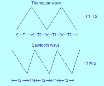
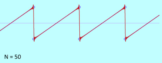
A waveform is a shape that represents changes in amplitude with respect to time. A periodic waveform includes sine wave, square wave, triangular wave, sawtooth wave. On the x-axis, it indicates the time and on y-axis it indicates amplitude. Many people frequently get confused between triangular wave and a sawtooth wave. The sawtooth wave generator is a one kind of linear, non sinusoidal waveform, and the shape of this waveform is a triangular shape in which the fall time and rise time are different. The sawtooth waveform can also be named an asymmetric triangular wave.
Sawtooth Wave Generator
A linear, non-sinusoidal, triangular shape waveform represents a sawtooth waveform in which fall time and rise time are different. A linear, non-sinusoidal, triangular shape waveform represents a pure triangular waveform in which fall time and rise times are equal. The Sawtooth Wave Generator is also known as asymmetric triangular waveform. The graphical representation of a sawtooth waveform is given below:
The applications of a sawtooth waveform are in frequency/tone generation, sampling, thyristor switching, modulation, etc.
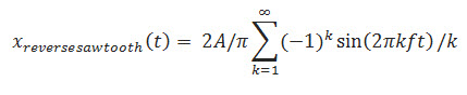
A non-sinusoidal waveform is nothing but a sawtooth waveform. Because its teeth look like a saw, it is named as a sawtooth waveform. In an inverse (or reverse) sawtooth waveform the wave suddenly ramps downwards and then rises sharply.
The infinite Fourier series is
A conventional sawtooth can be constructed using
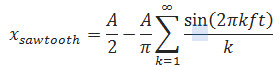
Where, A is the amplitude
By using a fast Fourier transform, this summation can be calculated more efficiently. In the time domain, the waveform is digitally created by using the non-band limited form. Sampling the infinite harmonics results in the tone that contains aliasing distortion.
Working Principle of a Sawtooth Wave Generator using 555
A sawtooth wave generator can be constructed using transistor and a simple 555 timer IC, as shown in the below circuit diagram. It consists of a transistor, a capacitor, a Zener diode, resistors from a constant current source that are used to charge the capacitor. Initially, let us assume that the capacitor is fully discharged. The voltage across the capacitor is zero and the 555’s output is high because of the internal comparators connected to the pin 2.
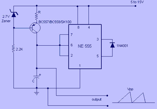
The capacitor starts charging to supply voltage because the internal transistor of 555 shorting the capacitor to ground and it opens. During charging, the 555 output goes low if the voltage increases above 2/3rd of supply voltage. During discharging, the 555 output goes high if the voltage across C decreases below 1/3rd supply voltage. Hence the capacitor charges and discharges between 2/3rd and 1/3rd of supply voltage. But the disadvantage is that it requires a bipolar power supply. The frequency is given by
F = (Vcc-2.7) / (R*C*Vpp)
Where,
Vpp- Peak to peak output voltage
Vcc- Supply voltage
To get the required frequency value, select the proper values for Vcc,Vpp, R, and C
Sawtooth Wave Generator using OP-AMP
A sawtooth waveform is used in pulse width modulation circuits and time-base generators. A potentiometer is used when the wiper moves toward negative voltage(-V); then the rise time becomes more than the fall time. When the wiper moves towards positive voltage(+V), then the rise time becomes less than the fall time.
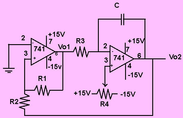
When the comparator output goes negative saturation, a negative voltage is added to the inverting terminal, thereby the wiper moves to a negative supply. This causes a decrease in the potential difference across R1 and hence current through the capacitor and resistor decreases.
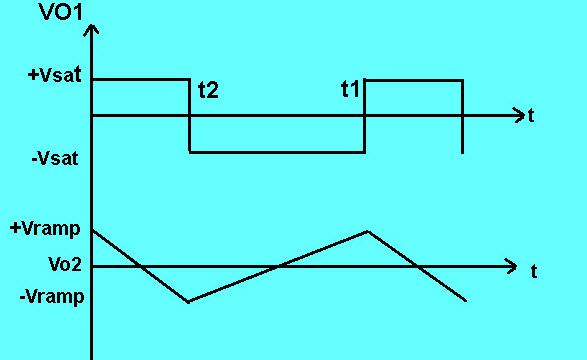
Then the slope decreases and rise time also decrease. When the comparator output is under positive saturation, the potential difference across the R1 increases and current through the capacitor resistor also increases. This is due to the presence of negative voltage at the inverting terminal. Then the slope increases and fall time decreases. And the output is obtained as a sawtooth waveform.
For wiring the circuit, the following are the components:
- Op-amp IC- 741c
- R-47K
- R1- 1K
- R2- 180Ω
What is a Sine Wave?
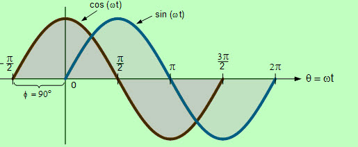
A mathematical curve that describes a smooth repetitive oscillation is said to be a sine wave or sinusoid wave. Often it occurs in pure and in signal processing as well as physics, chemistry, applied mathematics and in many other fields. It is the function of time (t).When added to any other sine wave with the same frequency, phase and magnitude, the sine wave retains its wave shape. It is known to be a periodic waveform that has this type of property. Such an importance leads its usage in Fourier analysis.
Y(x, t) = A sin (kx-ωt+Φ) +D
A is the amplitude
ω = 2πf, is the angular frequency
f is the frequency and it is defined as the number of oscillations per second.
Φ is the phase angle
D is non-zero center amplitude
ω = 2πf, is the angular frequency
f is the frequency and it is defined as the number of oscillations per second.
Φ is the phase angle
D is non-zero center amplitude
What is a Cosine Wave?
The shape of the cosine wave is identical to that of the sine wave except that the cosine wave exactly occurs ¼ cycles earlier than the corresponding sine wave. Sine wave and cosine wave have the same frequency, but the cosine wave leads sine wave by 90˚.
Y = cos x
Applications
- The sawtooth waveform is most common waveform used to create sounds with subtractive virtual and analog music synthesizers. Therefore, it is used in music.
- The sawtooth is the form of horizontal and vertical deflection signals that are used to generate a raster on monitor screens or CRT based television.
- The magnetic field suddenly gets collapsed on the wave’s cliff, which causes the resting position of its electron beam as quickly as possible.
- The magnetic field produced by the deflection yoke drags the electron beam on the wave’s ramp, creating a scan line.
- With much lower frequency, the vertical deflection operates in similar way as the horizontal deflection system.
- The stability of electronic components improves, and hence, there is no need to adjust the picture’s horizontal or vertical linearity.
- The positive voltage causes a deflection in one direction; the negative voltage causes the deflection in other, and the center- mounted deflection uses the screen area to depict a trace.
- The ramp portion must appear as a straight line; otherwise, it indicates the magnetic field, which is produced by the deflection yoke, as not linear,. This results in non-linearity and the television image is squished. Hence, on that side of the picture, the electron beam spends more time.
This is all about Sawtooth wave generator and its working principle. We believe that the information given in this article is helpful for you for a better understanding of this project. Furthermore, for any queries regarding this article or any help in implementing the electrical and electronics projects, you can feel free to approach us by connecting in the comment section below. Here is a question for you, what is the working principle of sawtooth wave generator?
A fully analytical steady state solution is presented for the problem of 3-D conjugate heat transfer in flip chip electronic packages with multiple general areal power sources, cooled by heatsinks using forced convection. The inherent simplicity of the proposed approach allows for expedient yet detailed package cooling/thermal analysis and evaluation of what-if scenarios while requiring only modest computational resources such as a personal computer. The soundness of the approach presented is demonstrated via excellent correlation with the results of experimental tests on flip-chip thermal test packages in a wind tunnel. The techniques developed herein are fairly general and can be readily adapted to other package designs wherein the primary heat transfer path is through the die, die-lid interface, lid, lid-sink interface and heatsink to the airflow through the fins. XXX , XXX 4%zero null 0 1 2 3 4 Pulse Width Modulation (PWM)
Use of PWM as a switching technique
Pulse Width Modulation (PWM) is a commonly used technique for generally controlling DC power to an electrical device, made practical by modern electronic power switches. However it also finds its place in AC choppers. The average value of current supplied to the load is controlled by the switch position and duration of its state. If the On period of the switch is longer compared to its off period, the load receives comparatively higher power. Thus the PWM switching frequency has to be faster.
Typically switching has to be done several times a minute in an electric stove, 120 Hz in a lamp dimmer, from few kilohertz (kHz) to tens of kHz for a motor drive. Switching frequency for audio amplifiers and computer power supplies is about ten to hundreds of kHz. The ratio of the ON time to the time period of the pulse is known as duty cycle. If the duty cycle is low, it implies low power.
The power loss in the switching device is very low, due to almost negligible amount of current flowing in the off state of the device and negligible amount of voltage drop in its OFF state. Digital controls also use PWM technique.PWM has also been used in certain communication systems where its duty cycle has been used to convey information over a communications channel.

PWM can be used to adjust the total amount of power delivered to a load without losses normally incurred when a power transfer is limited by resistive means. The drawbacks are the pulsations defined by the duty cycle, switching frequency and properties of the load. With a sufficiently high switching frequency and, when necessary, using additional passive electronic filters the pulse train can be smoothed and average analogue waveform recovered. High frequency PWM control systems can be easily implemented using semiconductor switches.
As has been already stated above almost no power is dissipated by the switch in either on or off state. However, during the transitions between on and off states both voltage and current are non-zero and thus considerable power is dissipated in the switches. Luckily, the change of state between fully on and fully off is quite rapid (typically less than 100 nanoseconds) relative to typical on or off times, and so the average power dissipation is quite low compared to the power being delivered even when high switching frequencies are used.
Use of PWM to deliver DC power to load
Most of the industrial process requires to be run on the certain parameters where speed of the drive is concerned. The electric drive systems used in many industrial applications require higher performance, reliability, variable speed due to its ease of controllability. The speed control of DC motor is important in applications where precision and protection are of essence. Purpose of a motor speed controller is to take a signal representing the required speed and to drive a motor at that speed.
Pulse-width modulation (PWM), as it applies to motor control, is a way of delivering energy through a succession of pulses rather than a continuously varying (analog) signal. By increasing or decreasing pulse width, the controller regulates energy flow to the motor shaft. The motor’s own inductance acts like a filter, storing energy during the “ON” cycle while releasing it at a rate corresponding to the input or reference signal. In other words, energy flows into the load not so much the switching frequency, but at the reference frequency.
The circuit is used to control speed of DC motor by using PWM technique. Series Variable Speed DC Motor Controller 12V uses a 555 timer IC as a PWM pulse generator to regulate the motor speed DC12 Volt. IC 555 is the popular Timer Chip used to make timer circuits. It was introduced in 1972 by the Signetics. It is called as 555 because there are three 5 K resistors inside. The IC consists of two comparators, a resistor chain, a Flip Flop and an output stage. It works in 3 basic modes- Astable, Monostable (where it acts a one shot pulse generator and Bistable mode. That is, when it is triggered; the output goes high for a period based on the values of the timing resistor and capacitor. In the Astable mode (AMV), the IC works as a free running multivibrator. The output turns high and low continuously to give pulsating output as an oscillator. In the Bistable mode also known as Schmitt trigger, the IC operates as a Flip-Flop with high or low output on each trigger and reset.

In this circuit, IRF540 MOSFET is used. This is N-Channel enhancement MOSFET. It is an advanced power MOSFET designed, tested, and guaranteed to withstand a specified level of energy in the breakdown avalanche mode of operation. This power MOSFETs is designed for applications such as switching regulators, switching convertors, motor drivers, relay drivers, and drivers for high power bipolar switching transistors requiring high speed and low gate drive power. These types can be operated directly from integrated circuits. Working voltage of this circuit can be adjusted according to needs of the driven DC motor. This circuit can work from 5-18VDC.
Above circuit i.e. DC motor speed control by PWM technique varies the duty cycle that in turn control the speed of the motor. IC 555 is connected in astable mode free running multi vibrator. The circuit consists of an arrangement of a potentiometer and two diodes, which is used to change the duty cycle and keep the frequency constant. As the resistance of the variable resistor or potentiometer is varied, the duty cycle of the pulses applied to the MOSFET varies and accordingly the DC power to the motor varies and thus its speed increases as the duty cycle increases.
Use of PWM to deliver AC power to load
Modern semiconductor switches such as MOSFETs or Insulated-gate bipolar transistors (IGBTs) are quite ideal components. Thus high efficiency controllers can be built. Typically frequency converters used to control AC motors have efficiency that is better than 98 %. Switching power supplies have lower efficiency due to low output voltage levels (often even less than 2 V for microprocessors are needed) but still more than 70-80 % efficiency can be achieved.

This kind of control for AC is power known delayed firing angle method. It is cheaper and generates lot of electrical noise and harmonics as compared to the real PWM control that develops negligible noise.
In many applications, such as industrial heating, lighting control, soft start induction motors and speed controllers for fans and pumps requires variable AC voltage from fixed AC source. The phase angle control of regulators has been widely used for these requirements. It offers some advantages such as simplicity and ability of controlling large amount of power economically. However, delayed firing angle causes discontinuity and plentiful harmonics in load current and a lagging power factor occurs at the AC side when the firing angle increased.
These problems can be improved by using PWM AC chopper. This PWM AC chopper offers several advantages such as sinusoidal input current with near unity power factor. However, to reduce the filter size and improve the quality of output regulator the switching frequency should be increased. This causes high switching loss. Another problem is the commutation between the transferring switch S1 with freewheeling switch S2. It cause the current spike if the both switches are turned on at the same time (short circuit), and the voltage spike if the both switches are turned off (no freewheeling path). To avoid these problems, RC snubber were used. However, this increases the power loss in the circuit and is difficult, expensive, bulky and inefficient for high-power applications. The AC chopper with zero current voltage switching (ZCS-ZVS) is proposed. Its output voltage regulator needs to vary switching-off time controlled by PWM signal. Thus, it is required to use frequency control to achieve the soft switching and the general control systems use the PWM techniques producing switching-on time. This technique has advantages such as simple control with sigma-delta modulation and continues input current.
XXX . XXX 4%zero null 0 1 2 3 4 Difference between Time Ratio Control and Current Limit Control
The industrial applications require power from the resources of DC voltage. Many of these applications, but, achieve better in case these are fed from adaptable DC voltage sources. The alteration of fixed DC voltage to a variable DC o/p voltage, the utilization of semiconductor devices is termed as chopping. A chopper is a fixed device, used to convert static DC i/p voltage to a variable o/p voltage straight. It is a high-speed ON/OFF semiconductor switch.For a chopper circuit, force commutated thyristor, GTO, power BJT and power MOSFET are used as the power semiconductor devices. A chopper may be thought of as the DC equivalent of an AC transformer since they perform in an identical manner like a transformer. A chopper is used to step up or step down the fixed DC i/p voltage. The chopper system gives high efficiency, smooth control, regeneration and fast response. There are two kinds of control strategies used in DC choppers namely time ratio controland current limit control.
Difference between Time Ratio Control and Current Limit Control
There are two kinds of control strategies used in DC choppers namely time ratio control and current limit control. In all situations, the average value of the o/p voltage can be changed. The differences between these two can be discussed below.
Time Ratio Control
In the time ratio control the value of the duty ratio, K =TON /T is changed. Here ‘K’ is called the duty cycle. There are two ways to achieve the time ration control, namely variable frequency and constant frequency operation.
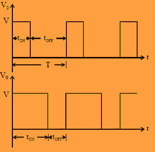
Constant Frequency Operation
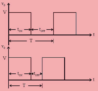
In constant frequency control strategy operation, the ON time TON is changed, keeping the frequency, i.e, f=1/T, or time period ‘T’ constant. This operation is also named as PWM (pulse width modulation control). Hence, the output voltage can be varied by varying ON time.
Variable Frequency Operation
In variable frequency control strategy operation, the frequency (f = 1/T) is changed, then the time period ‘T’ is also changed. This is also named as a frequency modulation control.In both cases, the o/p voltage can be changed with the change in duty ratio.
The disadvantages of Control Strategy include the following
- The frequency has to be changed over an extensive range of the o/p voltage control in FM (frequency modulation). The designing of the filter for wide frequency change is quite difficult.
- For the duty cycle ration control. Frequency change would be varied. As such, there is a possibility of intrusion with systems by positive frequencies like telephone lines and signaling in frequency modulation (FM) technique.
- The huge OFF time in FM (frequency modulation) technique may make the load current irregular, which is unwanted.
- Therefore, the constant frequency system with pulse width modulation is preferred for choppers or DC-DC converters.
Current Limit Control
In a DC to DC converter, the current value varies between the maximum as well as the minimum level of constant voltage. In this method, the DC to DC converter is turned ON & then OFF to confirm that current is preserved constantly between the upper limits and also lower limits. When the current energies beyond the extreme point, the DC-DC converter goes OFF.
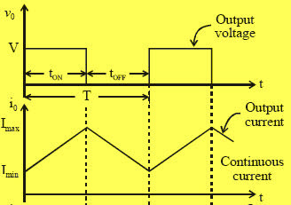
While the switch is in its OFF state, current freewheels through the diode and falls in an exponential manner. The chopper is turned ON when the flow of current spreads the minimum level. This technique can be utilized either when the ON time ‘T’ is endless or when the frequency f=1/T.
Thus, this is all about the differences between time ratio control and current limit control. From the above information, finally, we can conclude that DC-DC converters or choppers are presented along with the operation and its wave forms in each case. The different control strategies used in DC choppers are discussed. We hope that you have got a better understanding of this concept.Furthermore, any queries regarding this concept or to implement any electronic projects,
What is the Difference Between AC and DC Currents
In the today’s world electricity is most important next to the oxygen in the human. When the electricity was invented many changes have taken place over the years. Dark planet turned into a planet of lights. In fact, it made life so simple in all circumstances. All the devices, industries, offices, houses, technology, computers run on electricity. Here energy will be in two forms, i.e. alternating current (AC) and direct current (DC). Regarding these currents and the difference between AC and DC will be discussed in detail, its basic function and uses of it. Its properties are also discussed in a tabular column.
Working and Difference between AC and DC
The difference between AC and DC mainly includes the following
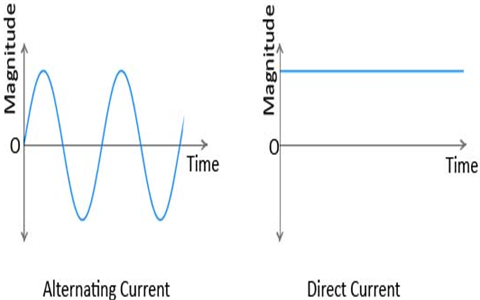
Alternating Current (AC)
Alternating current is defined as the flow of charge that changes direction periodically. The result obtained will be, the voltage level also reverses along with the current. Basically AC is used to deliver power to industries, houses, office buildings, etc.
Generation of AC
AC is produced by using called an alternator. It is designed to produce alternating current.Inside of a magnetic field, a loop of wire is spun, from which induced current will flow along the wire. Here the rotation of the wire may come from any no of means i.e. from, a steam turbine, flowing water, a wind turbine and so on. This is because the wire spins and enters into different magnetic polarity periodically, the current and voltage alternates in the wire.
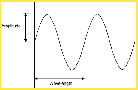
From this, the generated current can be of many waveforms like sine, square and triangle. But in most of the cases sine wave is preferred because it is easy to generate and calculations can be done with ease. However the rest of the wave requires an additional device to covert them into respective waveforms or the shape of the equipment has to be changed and the calculations will be too difficult. Description of Sine waveform is discussed below.
Describing a Sine Wave
Generally, AC waveform can be understood easily with the help of mathematical terms. For this sine wave the three things which are required are amplitude, phase and frequency.
By looking at just voltage, sine wave can be described like the below mathematical function:
V(t) = VP Sin (2πft + Ø)
V(t): It is a function of time a voltage. This means that as time changes our voltage also changes. In the above equation the term which is right of the equal sign describes how the voltage changes over time.
VP: It is the amplitude. This states how maximum the voltage the sine wave could reach in either direction, i.e. -VP volts, +VP volts, or somewhere in between.
The function of sin( ) states that the voltage will be in the form of a periodic sine wave and will act as a smooth oscillation at 0V.
Here 2π is constant. It converts the frequency from cycles in hertz to angular frequency in radians per second.
Here f describes the sine wave frequency. This will be in the form of units per second or hertz. The frequency tells how many times a particular waveform occurs within one second.
Here t is a dependent variable. It is measured in seconds. When the time varies the waveform also varies.
The φ describes about the phase of the sine wave. Phase is defined as how the waveform is shifted with respect to time. It is measured in degrees. The periodic nature of the sine wave shifts by 360° it becomes same waveform when shifted by 0°.
For the above formula, the real time application values are added by taking United States as a reference
Root mean square (RMS) is another small concept which helps in calculating the electrical power.
V(t) = 170 Sin ( 2π60t )
The other waves, i.e. triangle and square are shown below:
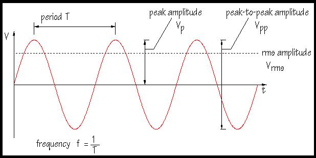
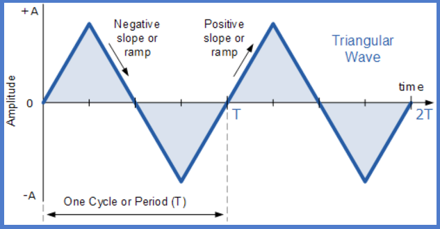
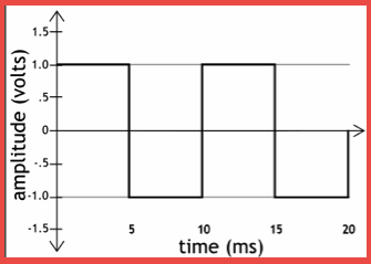
Applications of AC
- Home and office outlets are used AC.
- Generating and transmission of AC power for long distances is easy.
- Less energy is lost in electrical power transmission for high voltages (> 110kV).
- For higher voltages imply lower currents, and for lower currents less heat is generated in the power line which is obviously due to low resistance.
- AC can be easily converted from high voltage to low voltage and vice versa with the help of transformers.
- AC power the electric motors.
- It is also useful for many large appliances like refrigerators, dishwashers etc.
- Direct Current
Direct current (DC) is the movement of electric charge carriers, i.e. electrons in a unidirectional flow. In DC the intensity of the current will vary along with time, but the direction of movement stays the same in all time. Here DC is referred to voltage whose polarity never reverses.
DC Source
In a DC circuit, electrons emerge from the minus or negative pole and move towards the plus or positive pole. Some of the physicists define DC as, it travels from plus to minus.
Generally the basic source of direct current is produced by batteries, electrochemical, and photovoltaic cells. But AC is most preferred across the world. In this scenario AC can be converted to DC. This will happen in multiple steps. Initially, power supply consists of a transformer, which later converted into DC with the help of a rectifier. It prevents the flow of current from reversing and a filter is used to eliminate current pulsations in the output of the rectifier. The is the phenomenon how AC is converted into DC
Example of a Recharging Battery
However, all electronic and computer hardware to function they need DC. Most of the solid-state equipment requires voltage range in between 1.5 and 13.5 volts. Current demands vary accordingly with the devices which are used. For example the range from practically zero for an electronic wristwatch, to more than 100 amperes for a radio communications power amplifier. Equipment using, a high-power radio or broadcast transmitter or television or a CRT (cathode-ray tube) display or vacuum tubes require from about 150 volts to several thousand volts DC.
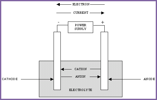
The main Difference between AC and DC is discusses in the following comparision chart
| S No | Alternating Current | Direct Current | |
1
| The amount of energy that can be carried | It is safe to transfer over longer city distances and will provide more power. | Practically the voltage of DC cannot travel very far until it begins to lose energy. |
2
| The cause of the direction of flow of electrons | It is denoted rotating magnet along the wire. | It is denoted steady magnetism along the wire |
3
| Frequency | The frequency of alternating current will be either 50Hz or 60Hz depending upon the country. | The frequency of direct current will be zero. |
4
| Direction | It reverses its direction while flowing in a circuit. | It only flows in one direction in the circuit. |
5
| Current | It is the current of magnitude which is varying with time | It is the current of constant magnitude. |
6
| Flow of Electrons | Here electrons will keep switching the directions – forward and backward. | Electrons move steadily in one direction or ‘forward’. |
7
| Obtained from | The source of availability is A.C Generator and mains. | The source of availability is either Cell or Battery. |
8
| Passive Parameters | It is Impedance. | Only Resistance |
9
| Power Factor | It basically Lies between 0 & 1. | It will be always 1. |
10
| Types | It will of different types like Sinusoidal, Square Trapezoidal, and Triangular. | It will be of Pure and pulsating. |
What Is the Difference between AC and DC currents is explained in detailed. I hope that every point is understood clearly about the alternating current, direct current, waveforms, about equation, differences of AC and DC in tabular columns along with their properties.
The φ describes about the phase of the sine wave. Phase is defined as how the waveform is shifted with respect to time. It is measured in degrees. The periodic nature of the sine wave shifts by 360° it becomes same waveform when shifted by 0°.
For the above formula, the real time application values are added by taking United States as a reference
Root mean square (RMS) is another small concept which helps in calculating the electrical power.
V(t) = 170 Sin ( 2π60t )
The other waves, i.e. triangle and square are shown below:
Applications of AC
- Home and office outlets are used AC.
- Generating and transmission of AC power for long distances is easy.
- Less energy is lost in electrical power transmission for high voltages (> 110kV).
- For higher voltages imply lower currents, and for lower currents less heat is generated in the power line which is obviously due to low resistance.
- AC can be easily converted from high voltage to low voltage and vice versa with the help of transformers.
- AC power the electric motors.
- It is also useful for many large appliances like refrigerators, dishwashers etc.
- Direct Current
Direct current (DC) is the movement of electric charge carriers, i.e. electrons in a unidirectional flow. In DC the intensity of the current will vary along with time, but the direction of movement stays the same in all time
ADP Motor Run Capacitors
ADP (Metalized Polypropylene) motor run capacitors are compact, self-healing products that find greatest utilization as motor-run capacitors in fractional horsepower electric motors. However, the motor run capacitors may be used in a wide variety of 50/60 Hz. AC or DC applications.
The motor run capacitors are available in capacitances up to 30 microfarads and with voltage ratings of 250, 370, and 440 VAC. The metalized polypropylene film dielectric provides excellent electrical characteristics including stable capacitance over time and temperature and a very low Dissipation Factor (internal heating).
The motor run capacitors’ integral mounting ear makes it an excellent choice for difficult to mount applications and the choice of terminal configurations is another big plus. Terminal configuration includes single or double 0.187 or 0.250 spade terminals fast-on, insulated wire leads, or PC-mount pins. ADP motor run capacitors can be supplied with a “lay-down” type bracket which provides additional mounting options. Other options available include P2 protected segmented film (ADP series).
ADP motor run capacitors offer UL, cUL, VDE, TUV, and CE approvals available. All ADP motor run capacitors are also RoHS compliant.
How to Make Flexible AC Transmitter System Using Thyristor Switch Reactance
FACTS is the acronym for Flexible AC Transmitter System. A Flexible AC Transmission System (FACTS) increase the reliability of AC grids. The IEEE defines FACTS as alternating current transmission systems integrating power electronics based and other static controllers to enhance controllability and power transfer ability. previously we have discussed “Need of FACTS and Types“
They improve power quality and transmission efficiency from generation through transmission down to the private and industrial consumers. In this article, we discuss Flexible AC Transmitter System Using Thyristor Switch.
Flexible AC Transmitter System by using TSR
A Flexible AC Transmitter System (FACTS) consists of static equipment which is used for AC transmission of electrical signals. It is used to increase controllability and to increase power transfer capability of an AC transmission system. This project can be enhanced by using firing angle control methodology for smooth control of voltage.
Flexible AC Transmitter System increases the reliability of AC grids and reduces power delivery cost. They also increase the quality of transmission and efficiency of power transmission.
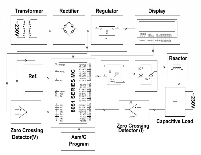
This method is used while charging transmission line or when there is a low load at the receiver end. When there are low load or no load, very low current flows through the transmission lines and the shunt capacitance in the transmission line becomes dominant. This causes voltage amplification due to which the receiver end voltage may become double than the sending end voltage.
To compensate this, the shunt inductors are automatically connected across the transmission line. In this system the lead time between the zero voltage pulse and zero current pulse duly generated by a suitable operational amplifier is fed to two interrupt pins of the microcontroller.
Types of Flexible AC Transmitter System Controllers
- Series Controller
- Shunt Controller
- Combined Series-Series Controller
- Combined Series-Shunt Controller
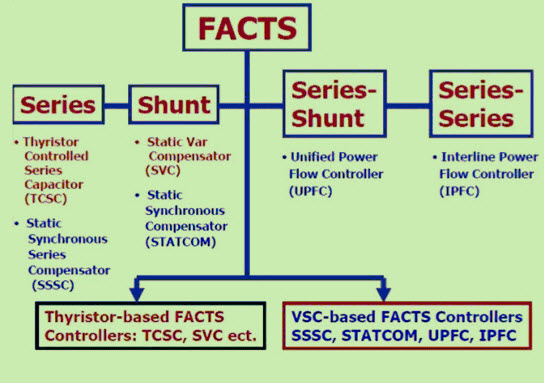
Thyristor
A thyristor is a four-layered, three terminal semiconductor device. The four layers are formed by alternate p-type and n-type semiconductors. Thus forming a p-n junction device. This device is also called as Silicon Controlled Switch (SCS) because of the silicon semiconductor in it and it is a bistable device.
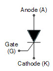
A thyristor is a unidirectional device and can be operated as an open circuit switch or as a rectifying diode. The three terminals of the thyristor are named as the anode (A), the cathode (K) and Gate (G).
The Anode is positive, the cathode is negative and the gate is used to control the input signal. It has two p-n junctions which can be switched ON and OFF at fast rates. The following shows the layers and terminals of the thyristor with its symbol.
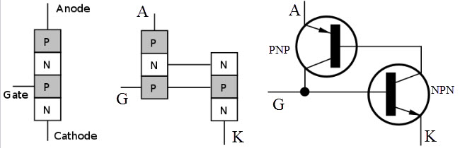
Thyristor has three basic states of operation
- Reverse Blocking
- Forward Blocking
- Forward Conducting
Reverse Blocking: In this mode of operation, the thyristor blocks the current in the same direction as that of a reverse bias diode.
Forward Blocking: In this mode of operation, the thyristor blocks the forward current conduction that is normally carried by a forward bias diode.
Forward Conducting: In this mode of operation the thyristor has been triggered into conduction. It continues conducting until the forward current drops below a threshold level called ‘holding current’.
Thyristor Switched Reactor
A thyristor switched reactor is used in electrical power transmission systems. It is a reactance connected in series with a bidirectional thyristor value. The value of thyristor is phase controlled, which allows the value of delivered reactive power to be adjusted to meet changing system conditions.
TSR can be used to limit the voltage rises on lightly loaded transmission lines. The current in TSR is varied from maximum to zero by varying the firing delay angle.
TSR can be used to limit the voltage rises on lightly loaded transmission lines. The current in TSR is varied from maximum to zero by varying the firing delay angle.
The following circuit shows TSR circuit. When the current flows the reactor is controlled by the firing angle of the thyristor. During every half cycle, the thyristor produces the triggering pulse through the controlled circuit.
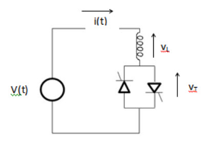
Circuit of TSR
A thyristor switched reactor is a three-phase assembly which is connected in a delta arrangement to provide partial cancellation of harmonics.The main thyristor reactor is split into two halves, with the thyristor valve connected between the two halves.
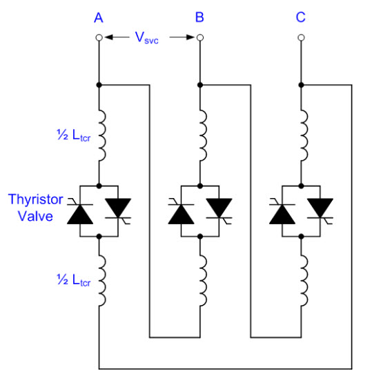
This protects the thyristor reactor circuit valve from damages due to flashovers and lightning strikes.
The main thyristor reactor is split into two halves, with the thyristor valve connected between the two halves.This protects the thyristor reactor circuit valve from damages due to flashovers and lightning strikes.
Operating Principle
The current in the thyristor is varied from maximum to zero by varying the firing delay angle (α). It is defined as the delay angle from the point at which the voltage becomes positive to the point at which the thyristor valve is turned on and the current starts to flow.
Maximum current is obtained when the α is 90o. At this point, TCR is said to be in full conduction. The RMS current is given by
Itcr-max = Vsvc/2πfLtcr
Where
Vsvc is the RMS value of the line to line bus bar voltage
Ltcr is the total TCR transducer for phase
The below waveform is the voltage and current of TCR.
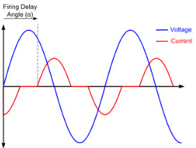
Advantages of Thyristor
- It can handle high current
- It can handle high voltage
Applications of Thyristor
- Used in electrical power transmission
- Used in alternating power circuits to control alternating output power.
- Used in inverters to convert direct current to alternating current
Applications of FACTS
- Used to control power flow
- Damping of power system oscillation
- Reduces generation cost
- Steady state voltage stability
- HVAC (Heating Ventilation and Air Conditioning) application
- Flicker Mitigation
I hope you have understood the concept of the flexible AC transmission system .
Modular Reconfigurable Robots in Space Applications
Robots are automatic electro-mechanical devices resembling humans or animals that are controlled by an electronic circuitry or computer program. There are different types of robots that are used for different types of applications. Recent trends in robotic technology have been developing advanced robots such as surgical robots are remote manipulators that are used for surgeries (especially keyhole surgery), walking robots that are mostly multi legged that are capable to move by walking, microbots and nanobots are microscopic and these nano robots or nano devices that are used in the human body to cure diseases, the rovers are robots with wheels that are used to walk on other planets for space exploration. Typically, robots used in space applications are autonomous robots, modular reconfigurable robots or self-reconfigurable modular robots, and so on.
Modular Reconfigurable Robots
Modular reconfigurable robots are generally autonomous kinematic devices with adjustable morphology. In fixed-morphology robots only the conventional tasks such as actuation, sensing and controlling are only able to perform. But, self-reconfigurable robots or modular reconfigurable robots are capable to change their own shapes by reorganizing their parts connectivity such that for adapting new circumstances, performing new tasks, and to recover from damages.
These self-reconfigurable robots can be defined as robots that can change their shape based on the path they have to pass through. For example, if a robot has to pass through a narrow pipe, then it will reconfigure itself in the shape of a worm and if it has to cross an uneven terrain, then it will reconfigure its shape with spider like legs. If there is a flat terrain, then it will reconfigure itself as a ball like structure for quick movement.
These reconfigurable robots are again classified into two types based on design. Such as homogeneous modular robotic systems consists of several modules with similar design to form a structure such that to perform a required task. A heterogeneous modular robotic system consists of several modules with different designs each of which performs specific functions and these are used to form a structure that performs a required task.
Reconfigurable Robots in Space Applications
As a part of research over the other planets, many countries are frequently launching several satellites or space missions to study the conditions and characteristics of the planets. Thus, for obtaining long term data, long term space missions are being launched and these long term space missions are typically self-reconfigurable systems.
These self-reconfigurable robots are capable of handling unforeseen situations and self-repair in case of any damages. We know that space missions are huge and mass constrained, so it is beneficiary if we use self-configurable robots that can perform multiple tasks instead of multiple robots that each perform only one particular task.
Till date, humans have set foot other than planet earth is only the moon. Whereas, modular robots used in space applications are being launched on many other planets. A series of landers, manipulators, orbiters, and rovers sent to Mars are famous robots used in space applications.
Robotic Manipulators and Rovers
There are various types of tasks that are performed by articulated robots in space. The process of servicing the apparatus or equipment in space is called as space manipulation which is done by articulated robots. Polybot suits well for space station or satellite maintenance and inspection. Robotic manipulators are projected for positioning in space or on other planets for emulating human manipulation abilities. They are generally positioned on free-flyer spacecraft or on orbit tuning of other spacecraft, within space vehicles, planetary landers, and rovers for acquiring samples.
Robotic rovers are projected for positioning on planets for emulating human movement abilities. They are frequently positioned on the terrestrial planets surfaces, small solar systems, aerobots (planetary atmospheres), cydrobots (ice layers), and hydrobots (liquid layers).
Automated Design and Optimization
Modular reconfigurable robots or modular robotic system is combined with software tools for assisting to select and design the finest morphology and control structure for performing each particular task. Although many traits of this design will unavoidably depend on human intelligence for the predictable future, other traits are acquiescent for automated design and optimization. All reconfigurable robots used in space applications must be designed such that capable to survive with launch stresses, radiation in the space, the vacuum, planetary distribution, and environment of the planet (planet on which reconfigurable robots are used or on target planets).
There are two types of designs of reconfigurable robots and they are: Lattice based designs and Chain based designs.
In lattice based designs, reconfiguration is easy, but it is hard to generate motion and this design requires more number of connectors and actuators.
In chain based designs, reconfiguration is hard and has insufficient stiffness, but it is easy to generate motion.
Modular Reconfigurable Robot Simulation
A software simulation environment based on physics, was developed using C++ that facilitates users for constructing reconfigurable robots utilizing a various types of modules. Additional module types are added with compatible connectors for extending the simulation.
Practical Example of Self-Reconfigurable Modular Robot
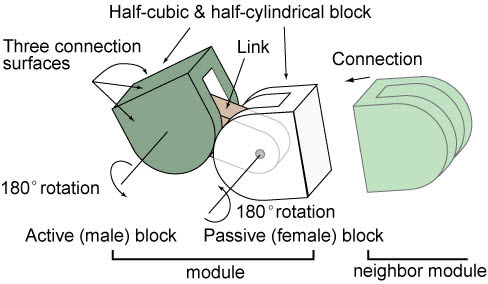
Modular transformer is one of the frequently used reconfigurable robots and these M-TRAN modules are used to form 3-D structure (that can change its own configuration and also capable to generate small robots), multi-DOF robot (that flexibly locomotes), and metamorphosing robot. This modular transformer consists of two actuators and battery.
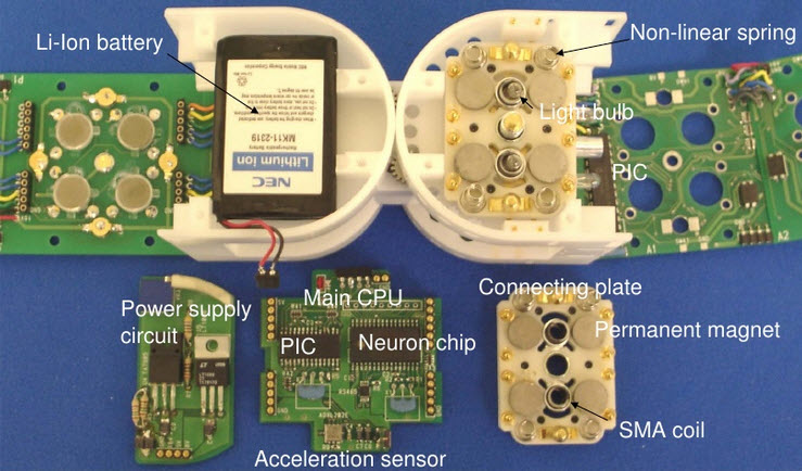
Internal block diagram of the M-TRAN module, it consists of Li-ion battery, non-linear spring, power supply circuit, main CPU, acceleration sensor, permanent magnet, SMA coil, connecting plate, and PIC.
These reconfigurable robots are used in space applications for achieving the specific goals such as telecommunication provision, observation over earth for data return, military feasibility, and navigation purposes.
There are many other robotic based projects and applications:
- Ultrasonic Obstacle Sensed Robotic Vehicle
- Robotic Vehicle Movement by Cell Phone
- Robotic Vehicle Operated by a TV Remote
- Track Sensing Robotic Vehicle Movement
- Fire Fighting Robot
- Voice Controlled Robotic Vehicle
- Pick N Place Robot Controlled by Android Wirelessly
- Metal Detector Robotic Vehicle
- Auto Metro Train to Shuttle between Stations
- RF Controlled Robotic Vehicle
- Touch Screen Based Remote Controlled Robotic Vehicle
+++++++++++++++++++++++++++++++++++++++++++++++++++++++++++
MATH <-------> HTAM FUNCTION LJBUSAF

+++++++++++++++++++++++++++++++++++++++++++++++++++++++++++
Tidak ada komentar:
Posting Komentar