robotic tool wrap so do robotic case packing toothpaste and electronics for ROBO ( Ringing On Boat ) AMNIMARJESLOW GOVERNMENT 91220017 PING HUNG LJBUSAF

 
                                                      ROBOTICS 


                                     


     

                                              


the basic elements of circuit design, with the goal of preparing you to design and build robotic sensors and control systems. The experience of designing and building is at least as important as gaining conceptual understanding. Therefore, this is a hands-on tutorial. Each concept is followed by a number of circuits to design and build, so that your confidence and understanding will have a solid foundation in actual skills.
The circuits and designs are all inexpensive, and may be built on a solder less breadboard with battery power, or with any 6 - 15V DC power supply.

An oscilloscope is an invaluable tool for learning circuit design -- it provides a way of seeing what is actually happening to your signals and wave forms. Unfortuantely, oscilloscopes are somewhat expensive. If you don't have access to a 'scope, it is possible to use the data-logging features of the Lego RCX in its place. For more on using the RCX as an oscilloscope,

Other useful tools include a cheap volt-ohm meter, and a basic logic probe.

Resistors

Voltage dividers are built out of resistors, so it's worth spending a moment looking at these basic components.
Most resistors look like this: IMAGE
And we tend to draw them like this:

Their resistance is measured in Ohms, (often in K Ohms for thousands of Ohms, or M Ohms for millions of Ohms. Their value is written on them with a color code.  Most resistors have a tolerance of 5-10%, but high precision ones are available. In general, it's a bad design that relies on an exact resistor value.
Many of us learned to recite Ohm's law in high school:

V = IR (voltage = current x resistance)

What may not have been emphasized then is that this law does not hold for most electronics components in general, but is more or less unique to resistors.  So, we can think of resistors as convenient current to voltage converters. 

Combining Resistors

We can combine resistors in series, and in parallel.
Resistors in series add values:

     R_total = R₁ + R₂ + ... + R_n

Resistors in parallel work a little differently. The general forumula for computing resistance in parallel is:

1/R_total = 1/R₁ + 1/R₂ + ... + 1/R_n

But this is formula a pain in the neck to work with. A slightly simpler transformaton, for two resistors, is:

     R_total = (R₁R₂)/ (R₁+R₂)

Even this, though, is not very usable. A handy rule of thumb for resistors in parallel is:

2 equal R's in parallel total R/2.
3 equal R's in parallel total R/3, etc.

As an example of how elegant this rule of thumb is, consider this arrangment of resistors:

To analyze it, take the two 10k's in parallel first -- they combine to make a 5k. Now you've got two 5k's in parallel, for a total of 2.5k ohms. Simple!
Here's another example, which makes the rule of thumb seem even more clever:

     =          =     

Instead of reaching for your calculator, think of the 5k as two 10k's in parallel. Now you've got three 10k's in parallel, for a total of 3.3k.
We have one other useful trick: spotting the dominating resistor. Remember that resistor tolerances are usually about 10%, so anything that changes our total resistance by less than 10% can be safely ignored.
In practice, this means we can ignore the effect of R_small in this case: 
And we can ignore the effect of R_big in this case: 
Assuming that R_big is more than ten times the value of R_small.

Resistor Challenge

Now it's time to do some hands-on work. Get a hold of:

• six or eight 1k resistors (brown-black-red)
• a solderless breadboard
• a volt-ohm-meter (VOM)
• needle nose pliers (handy, but not essential)

Become skilled at combining resistors by combining your 1k R's to make resistors of the following values on your breadboard:

• 333 ohms
• 3k
• 1.5k
• 667 ohms (extra challenge -- use only 3 resistors!)

Confirm your each of designs by testing them with the VOM.
Now get a 100k resistor. Put the 100k in parallel with a 1k, and measure ther result. Then put them in series, and measure the result. Which resistor dominates when?
By the way, it's good to work neatly on your breadboard. Use the needle-nose pliers to turn the resistor leads at sharp right angles, and then use the pliers to help slot them firmly into the breadboard holes. Make sure no leads touch each other above the breadboard. Neat construction habits will save you many headaches later on!

Voltage Dividers

Voltage dividers are aptly named -- they divide a voltage level into two parts. Dividers look like this:

This divider creates two potentials, across R1 measured from A to B, and another across R2 measured from B to C. (Incidentally, it's important to remember that a voltage is a difference, so we need to talk about voltages across two points, not voltages at single points.)
The voltages across R1 and R2 are proportional to the ratio of their values, and, of course the two voltages add up to V_in.
So, V_ab = V_inR1/(R1+R2) and V_bc = V_inR2/(R1+R2). But instead of memorizing this, get a feel for how dividers work by checking out a few examples.

	With equal resistor values, the input voltage is split evenly. Vbc is half of Vin: +6 volts. (Vab is also +6V.)
	When R1 is double R2, Vab is double Vbc. So, Vab is +8V, while Vbc +4V.
	R2 is five times R1, so Vab is one fifth Vbc. So, Vab is +2V, while Vbc is +10V.

Finally, it's worth looking at a variable voltage divider, made with a potentiometer. This is the sort of circuit used in places like a light dimmer, or a volume control on a radio. You might also see one used as an absolute angle sensor on a robot arm.

Divider Challenge

Even though the voltage divider looks simple, there are a few surprises in store when you atart to actually build them. For the first few, you'll use your VOM to test your circuits.
Set up your breadboard with +6V (or so) along the top power bus, and ground along the bottom bus (like this).
For each circuit, make a prediction about how it will split the voltage. Then build it and test them with your VOM. Remember that part of your job here is to get good at building with a breadboard, so take your time and work neatly.

	We'll start simple to get your feet wet. What should be the voltages across R1 and R2?
	This one shouldn't be much harder.
	This one looks easy to predict. But what happens when you measure the voltage across R1 and R2 with your VOM? If the results aren't what you expect, don't worry. We'll look at what's going on in the next section.

---

Now try two quick design problems:

• Design and build a divider to create a potential of 1.5V from your 6V source.



• Design and build a divider to create a potential of 0.15V from your 6V source. (Is this any more difficult?)

---

Finally, hook up this circuit, using a 10k pot. Use two VOM's to measure the Vab and Vbc. Turn the pot and see what happens as you measure both voltages at the same time. Impedance & Loading In the last challenge, we saw some strange behavior from this innocent looking divider: It looks like the voltage across R2 should be +3V. But when we measure it with a VOM, we get a value a good deal less than 3 volts -- hard to account for, since it's well outside the 10% tolerance of our components. Let's redraw the picture slightly to see what's going on: Now we can see what's going on -- R3 and R2 are in parallel! Together, they make a new, lower resistance value. Our when we attach the VOM, our circut is no longer a divider of two equal 10M resistors, but rather a divider of 10M and a smaller resistance. That's why the VOM measures a smaller voltage across R2 than we'd expect. Normally the resistance of the VOM is much larger than our R2, so there isn't a noticable difference when the VOM gets attached. But here, where the resistors in the divider are larger than the one in the VOM, the difference becomes a problem. We can generalize this result to talk about the problem of loading. Different circuits have different impedances -- which, for now, we can consider to be equivalent to their resistance. If we want our dividers to work the way we design them to, we should make sure that the impedance of each succesive stage is at least 10 times that of the previous one. Here's a bad chain of voltage dividers. The divider labeled B loads A, and C loads them both. Vout (the voltage between Vout and ground) is going to be hard to predict. Here, the designer followed the rule of making the impedance of each stage at least 10 times greater than the one before it. This gives us a much better chain of voltage dividers, which accomplishes the same idea as the one above while accounting for loading. The Vout here is easy to calculate. Divider A takes in 6V and gives 3V to B. B takes the 3V and gives 2V to C. C takes 2V and sends 1/3 of that, or 1.3V, to Vout. Everything works neatly when we account for loading and impedance. With this in mind, you might be tempted to design always using very low resistor values, like 1 or 2 ohms, for your voltage dividers. The problem with this comes back to V=IR. A divider with very low resistance will draw a lot of current. Excessive current draw will drain batteries quickly, cause overheating, and possibly damage more sensitive components. Later, we'll look at other ways of combating the impedance and loading issue using buffers. Loading Challenge We've got some new tricks in the bag. The first thing we can do is figure out the input impedance of the VOM. Make a divider with two 100k resistors, and use the difference between the measured and expected values to determine the impedance of the VOM. This challenge is easiest with a non-autoscaling VOM. Try different sensitivity ranges and see if they have different impedances. How do you think the VOM works? We can do the same trick with the LEGO RCX. Use 10k and 50k resistors to get 5V from a 6V battery. Feed that 5V to an RCX input port, and view the value on the RCX display. The RCX displays values from 0-5V as numbers from 0-1023. The 5V we're sending it should read 1023. Use the difference between the value we expect and the one we get to calcluate the RCX input impedance. In the Divider Challenge, we tried to make a divider that gave us 0.15V from a 6V source. This was hard because the resistor tolerances are 10%, and 0.15V looks like it stresses out our tolerances. Using our knowledge of loading and impedance, design a chain of voltage dividers that delivers 0.15V -- at least to within 10%. (Remember to account for the loading caused by the VOM.) RC Circuits Capacitors (or caps) are handy little devices made of two charge-carrying surfaces that are near each other, but do not touch. Some devices, like electric razors, use capacitors for their charge capacity. These end up using large capacitors like rechargable batteries. Capacitors have another quality besides their ability to store charge. Since they do not have a direct connection inside, caps block steady volatges. However, caps allow changing signals to pass through them. So, caps can be used as key parts of filtering circuits, and can remove unwanted frequencies from a signal. Sometimes this is handy for data acquisition. Other times, it's used to get rid of line noise or a DC voltage bias. Caps even help to smooth power supplies. We tend to draw caps one of two ways:  The symbol on the left is for an unpolarized cap, like the little brown ceramic capacitors. These caps don't care about polarity. The symbol on the right is for a polarized capacitor, like the electrolytic blue cylinders or yellow mylar caps. These do care about polarity, and will get destroyed if you connect the + end to a - voltage. It's curious that caps add capacity in parallel, while resistors add resistance in series. Conversely, resistors in parallel reduce resistance, while caps in series reduce capacity with the same formula. Luckily, it's not often that you'll need to calculate the value of a network of capacitors. Blocking Cap The first RC circuit doesn't use a resistor at all. A blocking cap is a capacitor that's used to remove any steady, DC bias of a signal. This is useful before amplification of a signal, where you don't want to amplify the bias. Here, the blocking cap removes a DC bias from the signal source, and delivers an unbiased signal to signal out.       Another way of thinking about the blocking cap is to say it removes the mean value from a signal. This can be handy when using statistical processes on the signal information. Blocking Cap Challenge If you have an oscilloscope and signal generator, use the signal generator to make a sine wave with a DC offset of about +5 Volts. View it on the scope while you play with the DC offset, and watch the waveform go up and down. Then, put a 1 micro-Farad capacitor in the signal path as a blocking cap. See how the signal jumps down to center around 0V? Play with the DC offset to see what happens -- also notice the effect of wiggling the DC offset quickly. What's going on? What happens to the waveform shape if you feed in a slow square wave? If you don't have a 'scope, you can still use the RCX. Write a Robolab program to turn a motor port on and off at full power as fast as possible. Feed this signal into one of the input ports, and use the datalogging feature of the RCX to view it. Then, feed the signal to the input port through a blocking cap, and notice the differences. Experiment with different size capacitors -- what changes? RC Time Constant When we charge a capacitor with a voltage level, it's not surprising to find that it takes some time for the cap to adjust to that new level. Exactly how much time it takes to adjust is defined not only by the size of the capacitor, but also by the resistance of the circuit. The RC time constant is a measure that helps us figure out how long it will take a cap to charge to a certain voltage level. The RC constant will also have some handy uses in filtering that we'll see later on. Calculating the RC is straight forward -- multiply the capacitance C, in Farads, by the resistance R, in Ohms. Remember to take care of your powers of 10 -- a micro-Farad is 10-6F, while a pico-Farad is 10-9F. In the circuits we'll look at, RC constants often come out to be in the hundreths of a second or millisecond range. Here's an RC circuit getting charged with a 10V source: Assuming the cap started with 0V, it's rise of voltage over time will look like this: The key points here are to note that after 1 RC, the cap will have reached about 2/3 of the V-in, and after 5 RC's, the cap will be very close to V-in. If, after charging the cap in our RC circuit to 10V, we brought V+ down to ground, the cap would discharge. And here again, the discharge time would be determined by the RC time constant. The RC curve for discharging looks like this: The key points on the discharge curve are at 1 RC, where the voltage is about a third of the original, and at 5 RC, where the voltage across the cap is nearly 0. Low Pass Filter One of the uses of RC circuits is filtering signals. Dr. Fourier tells us that every wave-form is really a composition of sine waves of different frequencies. The low=pass filter lets us filter out the high=frequency components of a signal, letting us focus on the low frequencies we may be interested in. A low pass filter looks like this:      You can think of it as a voltage divider that's frequency dependent. Or, you can think of the high frequencies traveling straight through the cap to ground, and the low frequencies bouncing off the cap and getting sent to Signal Out. The low frequencies keep most of their strength. The high frequencies are reduced. At a certain frequency, called f3db, the filtered strength of the frequency is exactly 3 decibels less than the original (or, about 70%). We can calculate f3db with this formula:   f3db=1/(2*pi*RC) So, if we know what frequencies we wish to filter out, we can choose an f3db accordingly. We can pick an R value to satisfy any impedance concerns, and then solve for the needed value of our capacitor C. High-Pass Filter A high-pass filter is similar to a low-pass filter, but the R and C swap positions. Now we can picture the high frequencies passing smoothly through the cap, while the low frequencies are rejected by it. (Although, again, thinking of the high-pass filter as a frequency dependent voltage divider may be more strictly correct.) Like the low-pass filter, the high pass filter also has an f3db point, defined by the same formula: f3db = 1/(2*pi*RC) Since this filter favors high frequencies, the graph of signal strength to frequency looks like this: With the low-pass and high-pass filters, we can accomplish a number of signal processing tasks, including selecting out a specific frequency band. We'll do more with this when we can include op-amps in our bag of tricks. Filter Challenge 1. Fourier tells us that a square wave is made of many sine waves of different frequencies. Use a low-pass filter to see if he's right. First, use a function generator or an RCX with Robolab to generate a square wave, and measure its frequency with a 'scope or RCX datalogging. Figure out where you'd put the f3db point of a low-pass filter to accept the fundamental frequncy of the square wave, while attenuating the higher frequencies. Then, design and make a low-pass filter with the R and C values set to that f3db value. Send the square wave through your filter and check out the results on the 'scope, or in Robolab. Do you get a pure sine wave? What's happening? What could you do to clean it up? 2. Fourier also tells us that the sharp corners of a square wave are built from very high frequency components. Design and build a high-pass filter with appropriate f3db to help you see the high frequency components prevalent at the corners of your square wave. What else do you see? Other Cap Uses Capacitors and RC circuits are useful for other things than just blocking and filtering. We'll mention a few of them briefly here: Timing. The RC time constant is used by many circuits, like the 555 timer we'll look at later on, to create steady clock pulses. These can be used for anything from flashing lights to driving simple computers. Smoothing. When converting AC line voltage to a DC power supply, caps are used to smooth out the bumps that come along with alternating current. Integrated Circuits. A small ceramic cap between the V+ and Ground pins of an integrated circuit helps it run better, and offers a bit of protection from line noise and brief power spikes. Calculus. When the f3db is low enough, a low-pass filter serves as an effective integrator, while a high-pass filter with a high enough f3db is a useful differentiator. These circuits work very well in combination with op-amps, as we'll see later.  Diodes Diodes are are the one-way arrows of electronics. Drawn sort of like an arrow, they allow current to flow only in the direction they're ponting. When you look at a diode, there will be a stripe around one end. This stripe is like the bar that the arrow points to. Current flows towards the stripe. So, it's important to pay attention to which way you put the diode into your breadboard. Normal diodes are used for rectifying signals and power supplies, and for clamping signals to a certain range. With an op-amp, a diode can be made to calculate logarithms. Finally, zener diodes are special diodes that can be used to establish convenient voltage levels. Diode Drop Strangely, the voltage difference across a diode is nearly constant, at about 0.6 Volts. This means that a diode is another component that pays no attention to Ohm's law. There are some applications where it's handy to have a .6V value, but mostly it's just important to remember that the diode drop is there in your circuit. Quick Challenge: Set up each of the circuits below. Use 1N914 diodes, or similar. Measure the indicated voltage levels with a VOM -- what do you expect to read?     Half-wave Rectifier Since diodes restrict the flow of current to one direction, they can be used to convert an AC power supply, which switches polarity from + to - many times a second, into a straight DC supply. The simplest rectifier uses one diode, like this: Called a half-wave rectifier, this circuit takes an AC signal in and chops off anything that falls below 0 Volts. Signal In:  Signal Out (Half-wave):  The half-wave rectifier is used in AM radios to rectify the signal. But for a rectifier in a power supply, it leaves something to be desired -- we lose half the power! Luckily, we can do better.

Full-wave Rectifier The half-wave rectifier chopped off half our signal. A full-wave rectifier does more clever trick: it flips the - half of the signal up into the + range. When used in a power supply, the full-wave rectifier allows us to convert almost all the incoming AC power to DC. The full-wave rectifier is also the heart of the circuitry that allows sensors to attach to the RCX in either polarity. A full-wave rectifier uses a diode bridge, made of four diodes, like this: At first, this may look just as confusing as the one-way streets of Boston. The thing to realize is that the diodes work in pairs. As the voltage of the signal flips back and forth, the diodes shepard the current to always flow in the same direction for the output. Here's what the circuit looks like to the signal as it alternates:     So, if we feed our AC signal into a full wave rectifier, we'll see both halves of the wave above 0 Volts. Since the signal passes through two diodes, the voltage out will be lower by two diode drops, or 1.2 Volts. AC Wave In:  AC Wave Out (Full-Wave Rectified):  If we're interested in using the full-wave rectifier as a DC power supply, we'll add a smoothing capacitor to the output of the diode bridge.

Rectifiers Challenge First, create an AC signal source. You can do by using a function generator with no DC bias. Or, you can take the output of an RCX pulsing a square wave, and run that through a blocking cap to remove the DC bias. View your signal to confirm that it crosses the 0V line symmetrically. Then rectify your signal, first with a half-wave rectifier, and then with a full-wave rectifer. Use 1N914 diodes, or something similar. View your output waves to make sure that the circuit behaves as it should. Can you see the diode drop? DC Power Supply Before, the output of the full-wave rectifier was bumpy. This will cause problems with our circuits if we try to use it as a power supply. So, to use the full-wave rectifier as a DC power supply, we'll add a smoothing capacitor to the output of the diode bridge. Now, the output of the power supply will be much smoother. We can reduce the size of the ripples by choosing a larger smoothing cap. The shape of the ripples is determined by the AC frequency and the RC time constant of the smoothing cap and circuit impedance. Zener Diodes Normal diodes let current flow with the arrow. But the Zener diode wants to be different. Zeners are designed to let current flow against the arrow. In the process, there is a consistent and very useful voltage drop across the Zener diode. We can use the Zener to give us a specific voltage whenever we need one. This is especially useful when a circuit requires an exact voltage in, but we're using a power supply that may be inconsistent, like batteries that drain over time. Zener's come in a range of values, including the handy 5.1 V Zener. Zener Challenge To get a feel for how the Zener diode works, set up this circuit on your breadboard: You can make a 12V supply by wiring two 6V's in series. Any 10k pot will do. You can use a 1N4733A diode, which is a 5.1V Zener. When you've built the circuit, turn the pot slowly and watch the volt-meter values. Meter A will show the voltage across the Zener, or Vout. Meter B will show the voltage across the pot, or Vin. Experiment a bit. How does the Zener react to quickly changing voltage levels? What happens when Vin drops below 5.1 Volts? Transistors Before 1947, amplification was done with large, hot vacuum tubes, and switching was done with large, hot relays. Then the transistor was invented by the good people of Bell labs, and suddenly electronics gained two new adjectives: small and cool. It's no an exaggeration to say that transistors formed the basis of the first great revolution in electronics that lead to micro-computing, consumer electronics, and practical robotics. Most of the circuits we use will not involve many discrete transistors. But transistors and their cousins lie imbedded in the tens or millions on the various chips we'll become familiar with. Learing about transistors will allow us to understand what's at the heart of them. To start, we'll note that transistors come in two flavors, NPN and PNP, and that each transistor has three terminals, the base, the collector, and the emitter. They look like this:   Transistor Switch We can think of a transistor first like a switch, controlled by a current running into the base. When the current is high enough, the switch turns on. Here, the control signal will turn power on and off to the load. Note that the load sinks current into the NPN transistor when it's made to act as a switch. To see this in action, try building this circuit: Use any small LED -- we'll only be giving it 5mA of current at 5V. The 2N3904 will work fine as a transistor, but the 2N4400 is designed better for the power loads of a transistor switch. The resistors are in the circuit to limit current. You don't need to put in a toggle switch if you build the circuit on a breadboard. Sticking a wire in and out of the breadboard will be just as good. Try it, and convince yourself that the LED only lights when there's current flowing to the base of the transistor. At first, it may seem like the transistor switch is no big deal -- why is it any better than just turning the LED on and off yourself? The key is that with a transistor we now have a switch that can turn other switches on and off. We can use it to build up networks of switches all the way into combinaional logic devices, digital memory, and full computers. The other good thing about a transistor switch is that it allows a small current to control a big one. In robotics, we often have low power devices, like micro-computers, controlling high power devices, like motors. The transistor switch allows the micro-computer to safely control the large currents required by the motors. Emitter Follower There are more subtle uses of transistors than the transistor switch. For these we need a more refined way of thinking about transistors. Where before we thought of them as a switches, now we can think of them as valves. Picture this valve controlling the flow of current the way a valve on a pipe controls the flow of water. Where before we just saw a transistor switch turn on and off, now we can see a transistor allow a little current to flow, or a lot, depending on how open the valve is. This idea allows us to construct a range of handy analog devices. The first of these is the Emitter Follower, which looks like this: The Emitter Follower sends a signal out that is equal to the signal in -- as long as the signal in is within the range of V+ to GND. So, if the circuit just sends out what you send in, what good is it? The utility of the emitter follower lies in impedance. The follower ends up solving many of the impedance issues that we found when trying to chain a series of voltage dividers or other loads. To the signal in, the follower looks like a high impedance device that won't attenuate the signal. To the signal out, the follower looks like a low impedance source that is easy to draw from. The follower makes it possible for us to chain many dividers or loads together without having to worry about their impedances. Transistor Challenge 1. Build a voltage divider with two 10M resistors, driven from a 6V source. Measure the voltage out of the divider with a VOM. What do you expect it to be? What do you measure? What causes the difference? 2. Now send the output of the voltage divider into an emitter follower. Use the VOM to measure the voltage output. What do you measure? Is it different than before? If so, why? Now, change the 10k resistor for a 1k resistor. Can you detect any changes in the circuit's behavior?   Op-Amps Op-Amps, or operational amplifieres are very high gain differential amplifiers set up to utilize the benefits of negative feedback. When we sort out what exactly this means, it'll become clear that they are fantastically useful little chips. Op-amps are drawn like this: The V+ and V- pins power the op-amp. These are also called the rails . Often times, circuit designers will leave the rails off of the diagram of an omp-amp circuit, but we need to remember to include them when we actually build them! The -Input is an inverting input -- think of it as multiplying the signal by -1 before processing. The +Input is non-inverting. We can use these pins together to create negative feedback loops, which make our circuits behave very nicely. Vout is the chip's output. We'll almost always feed a portion of the output back into the inverting input to create out negative feedback loop. We mentioned above that an op-amp has very high gain. When used without negative feedback, the amplifier's gain is somewhere from 1,000,000 to 10,000,000. Very small changes in the input signal would get maginified enormously. Negative feedback will reduce the amplifier's gain a great deal, but the benefit will be smooth amplification, free from distortion. Inverting Amplifier The easiest op-amp application to understand is the inverting amplifier, which looks like this: Notice two things. First, we left out drawing the power supplies, V+ and V- in the diagram, even though they're still in the circuit. This is common practice. Second, see that we're feeding a portion of the output back into the inverting input. This is the heart of the negative feedback loop, which will trades off a reduced gain for clean amplification. What is the gain of the inverting amplifier? It's easy to calculate: Gain = -R2/R1 (There's a clear, detailed explanation of exactly why this formula holds true, found in The Art of Electronics.) Let's take a look at an example circuit: Let's assume we feed it a sine wave that varies from +0.5V to -0.5V, and let's also assume for now that we're powering the chip with +10V on the V+ rail and -10V on the V- rail. What will the signal out look like? First, we'll calculate the gain. R2 is 10k, R1 is 1k, so the gain is -10. So our signals will look like this: This is pretty much as we expect -- the amplifier inverts the signal and multiplies it by ten. But what happens if we feed the same signal into the same amplifier, but change the power rails so that V+ is just +5V, and V- is now Ground (0V)? We're going to run into problems: Here, the output wants to go past the lower power rail of 0V, but gets clipped at about .7V. And it wants to go all the way to 5V, but gets clipped around 4.3V. This clipping happens when the power rails are set too close to the max and min of the output signal, and is something to watch out for. Non-Inverting Amplifier The inverting amp is a useful circuit, allowing us to scale a signal to any voltage range we wish by adjusting the gain accordingly. However, there are two drawbacks to it. First, the signal gets inverted, which can be slightly annoying -- although we can always invert it back with another op-amp. But the real drawback to the inverting amplifier is the amplifier's input impedance, which is equal to R1. As we saw with voltage dividers, we need to take a circuit's impedance into account when using it as part of a larger system of circuits. We need each successive circuit stage to have an input impedance at least 10 times greater than the output of the one preceeding it, to prevent loading. Since the inverting amplifier's input impedance is equal to R1, there may be times we'd be forced to pick unusually large resistors for our feedback loop, which can cause other problems. The solution to our impedance worries lie in the Non-Inverting Amplifier, also made with an op-amp and negative feedback: Here, the signal in goes directly into the non-inverting input, which has a nearly infinite input impedance -- perfect for coupling with any previous stage. Also, the output impedance of the op-amp is nearly zero, which is ideal for connecting with whatever comes next in the circuit. The formula for a non-inverting amplifier's gain is slightly different than the one for the inverting amp. For a non-inverting amp, the gain is: Gain = 1 + (R2/R1) Note that while the inverting amp can have a gain less than one for handy signal scaling, the non-inverting amp must have a gain of at least one. Naturally, we must still power the op-amp with V+ and V- giving enough range to comfortably accomodate our expected signal output. Using Chips Op-Amps are the first components we've used that are integrated circuits, which are also called IC's or chips. IC's are easy to use, but we need to know a few things about them. We'll be using chips that come in a DIP package, which has pins that plug right into our breadboards. Be careful not to order IC's that aren't in the DIP style, as these won't fit right. Static electricty can fry certain chips, especially those using what's called CMOS technology. Before picking up a chip, ground yourself by touching something grounded, like a radiator. Then, try to handle the chip without touching the metal pins. To insert a chip, put the pins across the trough in your breaboard, and gently push down until you feel it lock in. Be careful not to bend the pins. Each pin has a number. Pin 1 is identified by a dot, and is also to the left (looking down) of the notch on the casing. From there, the pin numbers proceed counter-clockwise. Use the datasheet of the chip to tell you what pin does what. For example, here's one from the 324A Op-Amp: Remember that every chip needs power. Connect V+ (also called Vcc) to your top power bus using a red wire. Use a black wire to connect V- to GND (0V), or a blue wire to connect V- to a voltage level below GND. Using the correct color wires will help you keep track of what's going on in your circuit. If your circuit is powered by a source with line noise, like a DC power supply that converts from AC, it's a good idea to put a small ceramic cap between the V+ and V-/GND pins of an IC. This cap will filter out the noise and make your chip work more reliably. Amplifier Challenge 1. Design an inverting amplifier with a gain of -20. Use an LF411 op-amp, or similar. Build your amplifier, and feed it with a .1V square wave, centered around 0V from a function generator or an RCX output, using Robolab. Where should you set the power rails, V+ and V-? Hint: if you're using the RCX, the output swings between 0-5V. Use a voltage divider to get the output from 0-.2V, and use a blocking cap to center the output around 0V. Remember to consider the output impedance of your divider in relation to the input impedance of the amplifier. Use a scope or RCX datalogging to verify the output of your amplifier. Try to overlay the input and output signals to verify that the amplifier inverts the signal. Then, if you have a scope, expand the time axis to look at the vertical edges of the square wave. Do the edges really rise straight up? What's happening? 2. Design a non-inverting amplifier, again using an LF411 or similar, with a gain of 10. Set the power rails at +5V/-5V, and drive the amp with a .2V sine wave if you have a function generator, or a .2V square wave from an RCX, voltage divider, and blocking cap, as above. Watch the output on a scope or RCX with datalogging. Then, drive the amp with a .5V wave. Can you see the clipping? How would you get rid of it? 3. Design a non-inverting amplifier with a gain of exactly one. What use could this have? Op-Amp Buffer So let's look at that third amplifier challenge problem -- design a non-inverting amplifier with a gain of exactly 1. Now, we could have done it with two inverting amplifiers, but there's a better way. We calculate gain for a non-inverting amplifier with the following formula: Gain = 1 + (R2/R1) So, if we make R2 zero, and R1 infinity, we'll have an amp with a gain of exactly 1. How can we do this? The circuit is surprisingly simple. Op-Amp Buffer Here, R2 is a plain wire, which has effectively zero resistance. We can think of R1 as an infinite resistor -- we don't have any connection to ground at all. This arrangement is called an Op-Amp Follower, or Buffer. The buffer has an output that exactly mirrors the input (assuming it's within range of the voltage rails), so it looks kind of useless at first. However, the buffer is an extremely useful circuit, since it helps to solve many impedance issues. The input impedance of the op-amp buffer is very high: close to infinity. And the output impedance is very low: just a few ohms. This means we can use buffers to help chain together sub-circuits in stages without worrying about impedance problems. The buffer gives benefits similar to those of the emitter follower we looked at with transistors, but tends to work more ideally. Buffer Challenge Someone is trying to create a set of voltage dividers that divides an input signal down to 1/12 of its original level. Here's what they've come up with so far: What's the problem here? Try driving the circuit with a square wave to confirm that there are impedance problems between the two divider stages. Then, design and build an improved version, using the same resistor values. One well placed op-amp buffer should do the trick. Confirm your design by driving the circuit with waves of several different amplitudes. Other Op-Amp Ideas Op-Amps are extremely handy for all sorts of analog signal processing tasks. The Art of Electronics spends some 90 pages going through them all. We'll take a quick overview of some of the more interesting op-amp applications for robotics here. You can play with the circuits to learn more about the ones that appeal to you, or look them up in Horowitz and Hill. Op-Amp Current Source This source provides a constant current supply to a circuit load. Note that the transistor current source is inside the feedback loop. Here, R1 and R3 make a voltage divider to set Vref, but Vref could be set by some other voltage signal, instead. The current is determined by the formula: Current Out = (V+ - Vref) / R2 Summing Junction The summing junction takes several signals and adds them together arithmetically. When all the R values are equal, each signal is given equal weight. If the R values are different, the output signal is a weighted sum, where the weight is inversely related to the R value. Although 3 input signals are shown in the diagram, the summing junction can handle as many inputs as you like. Typical Runit value is 10k. Note that the summing junction is an inverting amplifier, so your signal will get flipped around. Remember to use buffers on either end if impedance is as issue for your circuit. After all, op-amps are cheap. The summing junction allows us to do arithmetic on analog signals, like Output = 3X - 2Y. A basic use would be to allow one RCX input to process several different input signals. Sample and Hold The Sample and Hold circuit uses two buffers to keep a voltage level stored in a capacitor. Pressing Ssample will charge the capacitor to the present signal level, while the input buffer ensures the signal won't be changed by the charging process. From there, the output buffer will make sure that the voltage level across the storage cap won't decrease over time. Pressing Sclear will short out the storage cap, discharging it and setting the output to 0V. We can build the Sample and Hold circuit with mechanical pushbutton switches to see it in action. In actual practice, the switches used are various forms of transistor switch, which provides cleaner switching and also allows another circuit to control the sample and clearing operations. Excellent Sample and Hold circuits like the LF398 are available on a single chip for cheap and easy use. Sample and Hold circuits are used internally in Analog to Digital conversion. We might also use them to hold a given signal value from any particular sensor on a robot, for analysis and later use, especially if we don't want to bother encoding it and sending it to the CPU's memory. Integrator This circuit cleverly performs a bit of basic calculus on an input waveform, and outputs its integral as a voltage level. The exact voltage level is given by: where k is a constant. This circuit works quite well -- so well that it integrates small errors like random noise, and can soon float out of the output range. There are two ways of solving this problem. The first solution uses a very large resistor across the cap to drain off the errors accumulated by random noise: In the second solution, we have a switch that resets the integration from time to time. Pushing Sreset shorts out the cap to erase the errors. Here, we've drawn it as a pushbutton switch, but it could also be a transistor switch to allow for control from somewhere else in the circuit. A good use for an op-amp integrator could be as part of a position sensing system. Other Op-Amp Construction Challenge Take a look at the various circuits laid out in the previous section, Other Op-Amp Ideas, and find one that interests you. Design and build an example circuit that shows an application for the Op-Amp idea, and develop a convincing test to demonstrate its effectiveness. This challenge is more open-ended than some of the previous ones. It's a chance for you to get experience with the problems and possibilities of designing a circuit for a specific need, without a cookbook solution worked out by someone else. This is the first step to real fluency with electronics. Timing Circuits As we make the transition from analog to digital electronics, we need to first consider the issues of timing. All computers and robots require some sort of steady clock pulse, delivered by a timing circuit. The ultra-fast clock pulses of a computer are generated by an oscillating crystal. However, for our needs with robotics, we can be content with slightly slower and more flexible timing circuits. The timing circuits we'll look at will revolve around the use of the 555 Timer IC, a small, cheap chip that is rightly considered a true classic. 555 Timer The 555 Timer chip comes in many forms. We'll be using the handy 8 pin DIP package. We can use either the standard 555, or the 7555 which is a slightly improved CMOS version that is completely compatible with regular 555 circuits. The pin diagram of a 555 looks like this: And we tend to draw the 555 schematically in a box, like this: We'll often abbreviate the pin names to save space. Let's go through them one by one to understand what they do:

RC Curve Output To begin with the 555, let's hook it up in a standard configuration: As the circuit runs, let's examine the voltage levels across the capacitor -- that is, the voltage level between point X and Ground. Over time, the waveform looks like this: At first, this seems like a kind of peculiar waveform to be coming out of a circuit. But on closer look, we can see that it's the combination of two RC curves. The rising curve shows the cap charging, as it draws current through Ra and Rb, while the falling curve shows the cap discharging through the drain pin, sending current out only through Rb. The comparators inside the 555 are responsible for changing from charge to discharge when the voltage across the cap reaches 2/3 of the total Vcc, and from discharge to charge when the cap drops to 1/3 Vcc. Armed with this information, we can figure out the period T of the charge/discharge cycle, which is given by the formula: T = .693 C (Ra + 2Rb) For most purposes, changing .693 to .7 keeps us well within component tolerances. And of course, to get the frequency of oscillation, just recall that f = 1/T.

RC Curve Output Challenge 1. Design and build a 555 timer circuit with a slow period -- about 2 seconds. Use a volt-meter to measure the voltage across the capacitor C as you run the circuit. If your Vcc is +5 volts, what values should the meter read? 2. Design and build a 555 timer circuit with a period of about .3 seconds. View the voltage across the cap on your scope. Can you see the RC curve? Now, what should happen if you replace Rb with just a piece of wire? What should happen to the period? What should happen to the shape of the waveform? Try it to confirm.

Square Wave Output Now that we understand how the RC time constant controls the rate of oscillation for the 555, we can look at the more useful output, which is the square wave coming from the OUT pin. Where the waveform generated by the capacitor voltage varied between 1/3 Vcc and 2/3 Vcc, the square wave's amplitude goes all the way from 0V to the full Vcc. The period and frequency calculations for the square wave's HIGH-LOW cycle remain the same as before: T = .693 C (Ra + 2Rb)

Duty Cycle

If we look closely at the square wave graph, we'll notice that the output is HIGH for more than 50% of the time.

The ratio of time that the output is HIGH versus LOW is called the duty cycle. The way the standard 555 circuit is set up, we will always have a duty cycle that's greater than 50%.
To see why the output will be high longer than it is low, let's look at how current flows into and out from the capacitor:

It's clear that to charge, the RC circuit has two resistors in series, Ra and Rb. So, the charge time related to (Ra + Rb).
But the discharge path only flows through Rb. Therefore, the discharge time must be shorter than the charge time.
It might look at first like we could make a 50%-50% duty cycle by setting Ra to zero. However, we need there to be some positive resistance at Ra, to seperate the discharge pin from V+.
The circuit will function properly if we set Rb to zero. What will the resulting output waveform look like?

Square Wave Output Challenge

1. To get started, design and build a 555 circuit with a frequency of 1Hz. Examine the output on a 'scope, or using a voltmeter. How quickly does the voltage level change from HIGH to LOW.
Note: for this and the other 555 circuits, use a Vcc of between +5V and +6V.

---

2. Now, let's use the square wave to drive an LED. Hook the OUT pin of the 555 to the transistor switch we covered earlier. Set the 555 frequency to about 4Hz, and watch the LED blink happily.

---

3. Design and build a 555 timer with a frequency of 10Hz, and a duty cycle of 75%. Confirm your duty cycle by viewing the output on a 'scope.
Now, feed your output into a 74HC04 chip, like this:

Combinational Logic We now move from the realm of analog electronics, where signals can vary over a continuous range, to that of digital electronics, where signals are either HIGH or LOW. HIGH values are most often encoded as +5V, while LOW corresponds to 0V. This encoding allows us design natural, intuitive circuits that model formulas of boolean logic, as well as perform computations in the binary number system. We'll first look at strictly combinational logic circuits -- that is, circuits which respond to inputs, but lack the capacity for memory.

AND

We'll be doing our digital logic with logic chips, which are IC's with various logic gates embedded in them. These logic gates are built up of circuits similar to sets of the transistor switch we looked at before, but we don't need to worry about the individual transistors to use the chips as a whole.
The first gate we'll look at is the AND gate, which models the boolean conjunction ^. We draw AND gates like this:

We can describe the AND gate's behavior with a Truth Table, which maps all possible inputs to the output. We can give the inputs A and B either HIGH or LOW inputs, so the AND truth table looks like this:

A	B	Out
LOW	LOW	LOW
LOW	HIGH	LOW
HIGH	LOW	LOW
HIGH	HIGH	HIGH

In electronics, we often write formulas using the multiplication sign * in place of AND.
So, Y = A * B means Y equals A AND B.
AND gates come on chips of various sizes. One common chip series is the 74HCT series. The 74HCT08 is a quad AND chip, which has four AND gates on a single chip.

Note that in the pin diagram, 1A is input A for gate 1, 1B is input B for gate 1, and 1Y is output for gate 1.
Vcc should be close to 5V. A small ceramic cap between Vcc and GND will help keep the chip operating smoothly. Finally, make sure to tie any unused inputs to GND, as this will keep the chip from overheating.

OR

The OR gate models the boolean disjunction, V. We symbolize it like this:

The OR Truth Table shows that it outputs high when either input is high, or if they're both high.

A	B	Out
LOW	LOW	LOW
LOW	HIGH	HIGH
HIGH	LOW	HIGH
HIGH	HIGH	HIGH

Or is often writen with the + symbol. So, Y = A + B means Y equals A OR B.
The 74HCT0432 is a quad OR chip, similar to the quad AND from the last section.

 

NOT Finally, the last basic logic component is NOT, also called an inverter. In logical symbols, we denote NOT with a bar or ', so A' is the same as NOT A. The truth table for an inverter is pretty trivial: In Out HIGH LOW LOW HIGH Because the inverter is so common and so small, we often combine it with other gate symbols. Here, the NOT gets collapsed down to just a little circle. Note that here the corresponding formula is Y = A' * B. A hex inverter is a chip with 6 inverters in one casing. Here's the pinout for an 74HCT04 hex inverter: Now that we have command of AND, OR, and NOT, we can combine them to generate any formula expressible in boolean logic. For example, imagine we had to design a sensor that returns true when a robot is in the light and it's touching a wall, or when it's not light and it's not touching any walls. Also suppose there are 2 wall touching sensors, and one light sensor. We can begin by writing out our variables, with precise True/False definitions: TouchA = Wall Sensor A reports touching a wall. TouchB = Wall Sensor B reports touching a wall. LightOn = Light Sensor reports light is on. Now we'll write out a formula, using our variables and AND, OR, and NOT. Y = ((TouchA + TouchB) * LightOn) + (LightOn' * (TouchA' * TouchB')) Finally, we'll combine a series of gates to model the formula. Take the time to check through this diagram, and make sure you understand how the diagram reflects the formula. Note that there are some ways to simplify this gate diagram, but they may be slightly counter-intuitive. We'll examine some of those methods later on.

Basic Logic Challenge

1. First, take the time to verify that each gate does what it's supposed to do. Power up the chips with +5V, and use the following pushbutton setup to provide the logic levels:

You will notice that this set-up ties the logic level output to LOW when the button is not pressed, and sends it HIGH (because of the voltage divider) when the button is pressed. This eliminates the possibility of a floating input, that is not actively tied to either HIGH or LOW.
You can send the output of the logic chip to an LED (with 1k limiting resistor), or with a logic probe.
Try each of the gates, and make sure you can verify the truth table for each one.

---

2. Now, translate the following problem into a logical formula. Then, design a set of gates to model that formula. Finally, build the circuit, and test it using pushbutton inputs.
There's a company that needs a Good Taste sensor. The goal is to make an LED light when a piece of furniture is considered to be in good taste. There are three judges, each of whom has a push button. Judge A pushes her button when the furniture is brightly colored. Judge B presses her button when the furniture is old. Judge C presses her button when the furniture is really expensive.
The Good Taste sensor should light the LED if the furniture is brightly colored and not really expensive and not old; or if it's old and really expensive, and not brightly colored.

Max-Term Formulas

Sometimes, it can be tricky to reduce a situation into a logical formula. However, it's always straightforward to develop a truth table that reflects desired behavior. Once we have that truth table, there's a clear algorithm for describing it with a logical formula.
To make a truth table, first list all your variables in a row. Then list all possible states below them in rows. An easy way to do this is to count in binary, using 0 to mean LOW (or false), and 1 to mean HIGH (or true). Here's a three column example, with the boolean variables A, B, and C.

A	B	C
0	0	0
0	0	1
0	1	0
0	1	1
1	0	0
1	0	1
1	1	0
1	1	1

Now, go through every case and evaluate your situation, to see if it should result in a 1 (HIGH or true) value, or a 0 (LOW or false) value. We'll fill in values to model an arbitrary 3 variable boolean function.

A	B	C	Y
0	0	0	0
0	0	1	1
0	1	0	0
0	1	1	0
1	0	0	1
1	0	1	0
1	1	0	1
1	1	1	0

Now, to pull off a logical formula from the truth table, look at each row that results in a 1 output. Write all the variables down for that row, negating those with a 0 in their place with a '. AND these variables together with *'s. Since our example has 3 rows that result in 1's, we'll have three sets of these variables:

(A' * B' * C)
(A * B' * C')
(A * B * C')

Finally, OR each line together with a + to get the complete formula.

Y = (A' * B' * C) + (A * B' * C') + (A * B * C')

These formulas are called Max-Term formulas, because they look at rows in the truth table that give maximum values (1's). From here, it's an easy task to design the gates needed to produce corresponding circuit.
You may notice that while the resulting formula is always correct, it is not always the most efficient one possible. We'll spend a bit more time figuring ways of simplifying these formulas down.

DeMorgan's Rules

As we look at boolean formulas, it's tempting to see something like:

(A + B)'

and try to apply some sort of distributive property to it with the NOT, resulting in something like:

A' + B'

However, if you break down these two statements into truth tables, you'll find they're not equivalent. So, we can't blindly distribute NOT's around.
DeMorgan looked at this problem, and developed a set of rules for dealing with this idea correctly. His rules state that when you're negating a logical expression, you must both:

• Remove the ' from any negated variable, and add a ' to any non-negated variable
AND
• Flip + to *, and * to +

Using DeMorgan's rules, we can see that:

(A + B)' = A' * B'

And:

(A * B)' = A' + B'

We can apply DeMorgan's rules nicely to the following truth table:

A	B	C	Y
0	0	0	1
0	0	1	1
0	1	0	1
0	1	1	0
1	0	0	1
1	0	1	1
1	1	0	1
1	1	1	1

Here, we can see that pulling off a Max-Term formula will give us a very long boolean formula, since there are seven lines that result in 1 values.
We'll cheat, for a second, by focusing on the line that gives a 0 value for Y. We can say we get NOT Y from that line, and only that line. Let's write it out like this:

Y' = A' * B * C

So, it's also true that:

Y = (A' * B * C)'

Now, we can use DeMorgan to simplify:

Y = A + B' + C'

Which is much simpler than a seven line formula.
There are many other logical tricks for simplifying formulas. However, learning them all would be a full course of study in itself. So, for now, we'll be content with getting formulas and circuits that are correct, and at least not obviously inefficient.

Logic Design Challenge

Binary addition is pretty simple. 0+0 = 0. 1+0 = 1. 1+1 = 10. A Full Adder circuit takes three binary numbers, A, B, and C, and outputs two digits. The X digit is the one's place of the sum, while the Cout (or Carry Output) is the two's digit.
Below is the truth table for the X digit of the Full Adder.

A	B	C	X
0	0	0	0
0	0	1	1
0	1	0	1
0	1	1	0
1	0	0	1
1	0	1	0
1	1	0	0
1	1	1	1

Describe this table with a logical formula. Then design and build a set of logical gates to do the addition for the X bit.
Now, figure out the truth table for the Cout bit, and design and build a set of gates to do the addition for that bit. You now have a very simple calculator, that can do sums from 0 to 3.

---

Now, try a greater than or equals circuit. Given three inputs, A, B, and C, design and build a circuit that outputs true when the sum of A and B is greater than or equal to C. Write out a truth table first. DeMorgan may be useful here.

LOW True Logic

As we work toward circuits of greater complexity, it's worth pointing out that many computers and computational circuits are designed to make LOW values reflect the value True. Also called Active-LOW circuits, they are designed for lower power consumption.
For now, all we need to do is be able to spot LOW True logic when we see it. A LOW True pin will always have a little circle around it on the circuit diagram. And the pin label will often include a BAR or a ' sign, to indicate NOT. Together, it looks like this:

Here, we can see that WE' and RE' are both Active-LOW pins. To turn one of those pins on, we need to send it a LOW signal. And tying those pins to HIGH will keep them off.

Encoders & Decoders 1 of 8 Decoder Imagine we had 8 devices we wanted to control, but we wanted to keep the number of control switches to a minimum. One solution would be to use just 3 swithces, and interpret them as binary digits. A binary number 3 digits long can give us 8 values, from 0 to 7. It would be a straight-forward, but tedious, task to design a set of logic circuits to decode our 3 switches into 8 control signals. Luckily, there's a chip already produces that does the job for us. The 74HCT138 is a 1-of-8 decoder, which takes 3 bits of digital input and uses them to activate one of eight possible outputs. Let's walk through the chip pins. A, B, and C are the input pins. We can think of A as the 1's digit, B as the 2's digit, and C as the 3's digit. Note that these pins are LOW=True -- to encode a 0, send them a HIGH signal; and to encode a 1, send them a LOW signal. Y0-Y7 are the output pins. Again, these pins are LOW-True. So, when C is HIGH, B is LOW, and A is LOW, we'll be sending the number 011, or 3. That means that Y3 will send out a LOW signal, and all other pins will remain HIGH. There are also 3 enable pins, G1, G2A', G2B', which can disable the output pins. When G1 is HIGH, G2A' LOW, and G2B' LOW, the chip will operate as a normal decoder. But if we set G1 LOW, or either of G2A' or G2B' HIGH, then all of the outputs will be turned off, and output HIGH regardless of the inputs. These enable pins allow us to control the chip's output within the circuit. 8 to 3 Encoder Now, it may be that we want to get input from 8 different switches, but only have 3 inputs -- a common situation when working with the RCX, for example. Here, we could use an 8-to-3 Encoder. The 74HC148 encoder is one chip that will do the trick. Here, inputs 0-7 are the input signals -- again, these are Active-LOW. The chip encodes the input into a 3 digit output, A0 (1's bit), A1 (2's bit), and A3 (4's bit). EI enables the inputs. When it is LOW, the chip works properly. When it's HIGH, all outputs are set to HIGH regardless of the input. EO and GS are outputs that we can ignore for now. The encoder and decoder chips allow us to maximize the use of inputs and outputs. Since the RCX has only 3 of each, it's handy to be able to get more than 3 pieces of information back and forth at any one time.

Digital Multiplexers Consider a situation where we have many possible input devices, but only want to look at one input at a time. This is a job for the multiplexer, which selects one of many inputs, and sends that value to the output. Schematically, an 8 input multiplexer looks like this: The selector inside the MUX gets a code from the 3 Address bits, A0, A1, and A2. It then chooses the appropriate input, and channels that input value to the output. We can use a MUX not only to channel various input devices to a singal output, but we can also use them to implement arbitrarily complex truth tables. Here's one example: A B C Y 0 0 0 1 0 0 1 0 0 1 0 0 0 1 1 1 1 0 0 1 1 0 1 1 1 1 0 0 1 1 1 0 To use the MUX as a truth table, just connect the input for a given address to HIGH if that line in the truth table is 1, and to LOW if it's a 0. (Assuming an active-HIGH circuit.) Multiplexers come in many shapes and sizes. One common 8 input MUX is the 74HC251. Here, the inputs are labeled I0 through I7, the address selectors are called S0, S1, and S2, and the output is Y. Y' outputs the opposite of the selected data. OE' is the Output Enable. Set OE' to LOW to activate the chip. We'll talk more about output enabling when we get to the idea of the data bus.

Logic Network Challenge 1. Design and build a circuit to deliver the inputs of 8 different switches into the Lego RCX, using an encoder. 2. Design and build a circuit to light any 1 of 8 LED's, and drive it with the 3 outputs of the Lego RCX. 3. Assign prime numbers to each of the buttons you built in part 1, and label the LED's from part 2 with numerals 0-7. Write a Robolab program that allows the user to select two prime numbers P1 and P2 by pressing two buttons, one at a time. The program should output the result of the operation (P1 * P2) MOD 8. 4. Use a 4 input MUX to implement the truth table for a circuit that models XOR -- the exclusive-or function that is modeled by the formula: Y = (A * B') + (A' * B)

Flip-Flops and Counters Up until now, our digital circuits have been strictly combinational -- they take inputs and react to them. While they are capable of complex calculations, they lack the ability to remember what they've done. This lack of memory severly restricts the capabilities of the circuits we can design. The flip-flop is the basic unit of digital memory. A flip-flop can remember one bit of data. Sets of flip-flops are called registers, and can hold bytes of data. Sets of registers are called memories, and can hold many thousands of bits, or more. The basic flip-flop circuit is the classic set of cross-coupled NAND gates. Since nobody buils flip-flops from the gate level anymore, we'll skip past this level of analysis, and move straight into the chips we'll actually use. But if you're interested, The Art of Electronicsdevotes many pages  to the inner workings of flip-flops, from the cross coupled NAND's on up.

D-flops One of the most common kinds of flip-flops (or, just flops) is the D-type flop. Like all flops, it has the ability to remember one bit of digital information. What makes the D-flop special is that it is a clocked flip-flop. We'll spend some time looking at what that means. First, let's go through the pins of a standard D-flop. The diagram above is for half of a 74HCT74 chip, which comes with two D-flops on one IC. D is the Data Input pin. This is where the flop gets its information from. Q is the Output pin. It shows what value the flop is currently remembering. Q' is the Inverted Output pin. It shows the opposite of the value that the flop is remembering. CLK is the clock pin. When a new clock pulse comes in, the flop checks the input pin D, and sets itself up to remember that input value. The D-flop is edge-triggere, which means that it responds to the rising edge of the clock pulse. This will be clearer when we look at a timing diagram, below. R is an Active-LOW Reset pin. When the Reset pin gets a LOW signal, it resets the flop to remember a 0, or LOW value. S (also called PRE on some diagrams) is an Active-Low Set pin. When it gets a LOW signal, it sets the flop to remember a 1, or HIGH value. The flip-flop is the foundation of sequential logic. To understand how to use flops, we need to see how they function over time in reponse to different signals. We'll walk through a sequence, using a timing diagram to help show what's going on. At the beginning of the diagram, the inputs to the D and CLK pins are LOW, and the Q output also happens to be LOW. At point A, the D input goes HIGH. However, since there is no clock pulse, the Q output does not change yet. At point B, the CLK input sees a rising edge. That rising edge tells the flop to remember the D input. A very short time passes from point B to point C, which is the time needed to actually make the flop remember the new value. Note that now the Q output is the same as the D input. At point D, the D-input goes to LOW. However, the Q output does not change, because there is no clock pulse. At point E, we have a falling edge on the CLK input. However, our flop only responds to rising edges, so the output Q still persists. Note that the S and R pins will Set or Reset the flop regardless of the D input or clock pulses. These pins are often used to set the flop to an initial state before our logic circuits begin their work. Here's the pinout of the 74HCT74N, a dual D-type flip-flop. Note that the 'dual' designation means that two flops come on one chip.

Switch Debounce Having a component with memory can help us design circuits to solve a real variety of problems. To see how flexible flops are, we'll look at the problem of switch debounce. Consider this circuit, which is a fairly standard design for getting digital input from a push=button: Now imagine what happens when we actually push button. We'd like the signal to have a sharp transition from LOW to HIGH, so it would look like this: However, since the button is made of physical materials like metal, there will be some elastic vibrations, which result something like the following signal: That switch bounce can wreak havoc on our edge triggered digital circuits, which can and will interpret each of the tiny peaks in the switch bounce as a new signal pulse. We could get rid of the bounce by using a low-pass filter. However, this would slow down our response time, since we'd now have to allow for the RC curve. Instead, we'll feed the output of our physical switch into a D-flop, and clock the flop with regular pulses from a 555 timer. The timing diagram of the switch debouncer will look something like this: The clock pulse should be fast enough to catch the shortest possible switch pressing, but slow enough not to be confused by the switch bounce, which typically lasts for about 1ms. So, if we feed the flop with square waves that have a period of 1.5ms, we'll satisfy both constraints.

Registers

One handy thing about flip-flops is that we can pack them onto chips pretty tightly. When we put 8 flops onto one chip, we have what's called a register. An 8-flop register can hold one byte of digital information.
Registers are very similar to normal D-flops, with a few differences. Here's a schematic diagram for a D-register:

Naturally, the D0 input feeds the Q0 output, and so on. You'll notice that all 8 of the D-flops are driven by a single clock input, marked with the triangle. They also share a single Reset pin. Registers make it handy to work with whole bytes at a time.
Often, we'll feed a register with inputs from a Data Bus. We'll talk more about the idea of the Data Bus later, but for now, we'll see that we don't have to draw 8 seperate lines when we're feeding a byte into a register. Here's a convient schematic for an 8-bit bus:

The convention is that D0 will represent the lowest order (smallest) data bit, while D7 will represent the highest order (largest) bit.
Here's the pinout for an 74HCT273 register:

Flip-Flop Challenge

1. First, set up a pushbutton switch to deliver a logic level input. View its output on a scope, and look at the switch bounce. Measure the duration of the switch bounce.
Then, set up a 555 timer that outputs a square wave with a period of 1.5 times the duration of the bounce for your switch. Finally, use that timer to drive a D-flop that debounces your switch. Use one of the flops on a 74HCT74N chip. View the debounced output on your scope next to the input. How much time delay is there between the input and output signals?
Make sure to tie S and R inputs HIGH (inactive).

---

Now, get ahold of a 74HCT273N D-register. Use the output of your debounced switch to clock the register. Attach 8 logic-level input switches to the D inputs of your register. Attach LED's, or a 7 segment LED to the Q outputs of your register. Remember to tie the R reset HIGH (inactive).
Experiment with your new circuit by pressing down different input buttons and then clocking your register with the debounced switch.
Then, add a logic level input switch to the R reset input. This input should be normally HIGH, but should output LOW when the switch is pressed. Experiment with this Reset button. Which takes priority for the chip, the clock pulse or the reset pulse?

Divide-by-2 Counter Although it may seem obvious to say so, we can't count unless we have some kind of memory. The Divide-by-2 Counter is the first simple counter we can make, now that we have access to memory with flip-flops. Here's the basic circuit: Here, we're feeding the inverted output Q' into the D input. This means that every time we get a rising edge on the clock signal, our output will flip states. So, clearly there's some division going on. But how do we interpret this as counting? Let's look at what happens when we assign numbers to the voltage levels. 0 = LOW, 1 = HIGH. Now, if we interpret the Clock levels as the 1's bit, and the Q out as the two's bit, we can see we've got a binary counter that counts from 0 to 3, and then resets. So, our Divide-by-2 counter allows us to count clock pulses in a meaningful way. However, with one D-flop, we've got a severe limit on how high we can count. We need to find ways of counting past 4 if these circuits are going to be useful.

Ripple Counter A good first thought for making counters that can count higher is to chain Divide-by-2 counters together. We can feed the Q out of one flop into the CLK of the next stage. The result looks something like this: The ripple counter is easy to understand. Each stage acts as a Divide-by-2 counter on the previous stage's signal. The Q out of each stage acts as both an output bit, and as the clock signal for the next stage. We can chain as many ripple counters together as we like. A three bit ripple counter will count 23=8 numbers, and an n-bit ripple counter will cound 2n numbers. The problem with ripple counters is that each new stage put on the counter adds a delay. This propagation delay is seen when we look at a less idealized timing diagram: Now we can see that the propagation delay does not only slow down the counter, but it actually introduces errors into the system. These errors increase as we add additional stages to the ripple counter.

Clocked Counters

To solve the problems of propagation delay introduced by the ripple counter, we'll use a synchronized counter. The synch'd counters are set up so that one clock pulse drives every stage. Since synch counters are readily available as cheap IC's, we'll move straight on to talk about how to use a counter chip.
A counter chip comes with a fair number of features on it. Here's the pinout for a 74HC193, which is a 4-bit binary up/down counter with load and clear.

Let's have a look at the different pins.

Counters Challenge

1. Set up a Divide-by-2 counter using one D-flop from a 74HCT74N chip. Drive the counter with a square wave from a 555 Timer that you've set up to have a period of about half a second. Drive a red LED with the 555 Timer's square wave, and a green LED with the Q output from the D-flop.
At what rate should the green LED blink? How can we interpret the green and red LED's as numbers?

---

2. Add two more stages to the Divide-by-2 counter from above, making a 3-bit ripple counter. Drive an output LED with each Q outout, and watch it count happily.
Now, use a scope to watch two of the Q outputs. Expand the time axis to see the propagation delay. How much delay is there per stage?

---

3. Set up a synchronous counter using an SN74HC193N chip, or similar. Drive the UP and DOWN counters with straight (not-debounced) logic-level pushbutton inputs. Drive LED's from the Q-outputs.
Click along with your pushbutton UP. What problems do you find using a not-debounced switch to clock the counter?

---

4.Add a debouncer to the UP clock. Design and build a Divide-by-5 counter, using only the SN74HC193N, and the debounced UP input. The Divide-by-5 counter should light an LED every 5th time the user has pressed the UP pushbutton.
Hint: you'll need to use the LOAD' function of the chip, in conjunction with CO'. 

Micro-Controllers

A micro-controller is a small, programmable computer that's capable of sending logic level signals in and out of numerous pins. A micro-controller allows us to embed a full computer within a circuit. This allows us to easily design systems of great functional complexity.
Micro-controllers also offer a handy short-cut for making normal combinational logic circuits and sequential logic circuits. They're so flexible and easy to use that sometimes it almost feels like cheating.
If you've used a Lego RCX, you've already encountered a micro-controller. The RCX has a version of the Hitachi-8 chip at its core -- the rest of the RCX system is basically just power supply and user interface.
PIC chips are a series of mirco-controllers that are available in a dizzying array of size, memory, and number of pins. They've become one of the industry standards, and compilers are available to program them in a variety of languages.
The BASIC Stamp is a PIC chip that has been housed in a handy user interface. The BASIC Stamp II (also called a 'Homework Board') is available from parallax.com. Instead of requiring us to learn assembly language, the BASIC Stamp family allows us to program a micro-controller in a friendly, intuitive language.
We'll spend some time here looking at a few different things we can do with a full mirco-controller like the BASIC Stamp II. This section will not attempt to duplicate the excellent documentation, such as the Basic Stamp Programming Manual available at the parallax.comwebsite, but will instead help get you started with a series of challenges.

Button Challenges

We'll start by setting up two simple circuits, driven by Stamp Pins. One is a standard logic-level push-button, the other is a straight LED output. We'll use these two pieces for the first set of challenges.

You'll notice that the BASIC Stamp Homework Board comes with a small breadboard and pins. The Vdd pins correspond to +5V. The Vss pins correspond to GND. The input/output (i/o) pins are marked P0 to P15. You can use any i/o pins you like, so long as you keep track of what's what.

---

1. Use the BUTTON and TOGGLE commands to write a program to toggle the LED on and off. Every time the user presses the button, the LED should switch from on to off, or off to on.
Note that the BASIC Stamp takes care of debouncing your switch for you. Brilliant!
2. Use the BUTTON, IF, WHILE, HIGH and LOW commands, in conjunction with a word-length variable, to make a system that measures how long the user presses the button. The system should then PAUSE for a short time, and then light the LED for the same length of time that the user pressed the button.
What problems may occur if the user presses the button for a very long time? How could we combat this?

Logic Challenges

For these challenges, set up three logic-level push-button inputs. Also set up a Green LED and a Red LED for output.

---

1. Write and run a program that lights the Green LED if exactly one button is pushed, the Red LED if exactly two buttons are pushed, and lights both Red and Green if all three buttons are pushed. If no buttons are being pushed, the LEDs should be off.

---

2. Write and run a program for a Loan Approver. The three buttons should represent the following conditions:

• A -- the applicant is steadily employed
• B -- the applicant has strong credit
• C -- the applicant is a graduate student

The Green LED should light if the applicant is steadily employed and has strong credit. The Green LED should also light if the applicant is steadily employed and is a graduate student.

However, if the applicant ever claims to have strong credit and be a graduate student, then surely the applicant is a liar, and the Loan Approver should call for Sxecurity by blinking the Red and Green LEDs back and forth. The Approver should light the Red LED on any other combination of inputs, and should turn the lights off if no button is being pressed.

Sensors

Sensors allow our circuits to get information from the outside world. Many of our circuits have already used the simplest sensor -- the pushbutton switch. The pushbutton switch is fairly crude, in that it does not offer much in the way of resolution. It can tell us if someone (or something) is pressing it, but it can't tell us how hard, or who it might be.
Most sensors fall into one of three basic categories. There are those sensors that change resitance to convey informatio, those that provide a change in voltage, and finally those that deliver digital information and describe their sensory information with numbers.

Variable Resistance Sensors Some friendly sensors provide information in the form of a changing resistance. Pot's are sometimes used in this way as absolute angle sensors. Thermal resistors change resistance with temperature. And pressure sensors work by changing resistance in repsonse to pressure. With any of these devices, the trick is to figure out how to make our circuit recognize what the resistance value is. If we're using a BASIC Stamp, we can use the RCTIME command, with an RC circuit set-up. Choose a cap value that gives a reasonable range of RC time constants for your expected range of resistances. If, on the other hand, we're using a Lego RCX, we can have the RCX read the resistance as a sensor. The RCX converts an external resistance into a RAW value (between 0-1023), with this formula: RAW = 1023 * R / (10000 + R) Where does this formula come from? There's a 10k pullup resistor inside the RCX, so your R and the 10k resistor are in parallel. The formula calculates the parallel reistance (10k * R)/(10k + R), and then scales that parallel resistance to the desired range(1020/10k).

Variable Resistance Challenge

Make a pressure sensor using anti-static foam, which comes with most IC chips. Put a chunk of the anti-static foam between two pennies, and solder wires to the outsides of the pennies. Wrap the whole thing in electrical tape to keep it together.

---

1. Test your pressure sensor by measuring the resistance values you get under different pressures, using a VOM.

---

2. Hook up the pressure sensor to a Lego RCX, which drives a robot car. Write and run a program that allows the user to squeeze the pressure sensor to determine the car's forward speed.

---

3. Hook up the pressure sensor to a BASIC Stamp, using an RC circuit. Hook up a 7 segment LED display. Write and run a program that outputs the sensor's pressure on a realative scale from 0-9 on the LED display.

Digital to Analog Conversion

For now, check out the RCX digital interface


                                                  XXX  . XXX  Packing ROBOTICS  


                                            

Packing Robots

(877) 759-8151

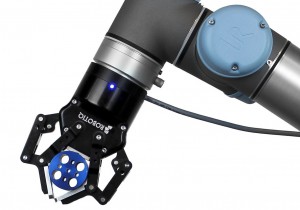
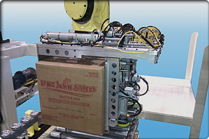
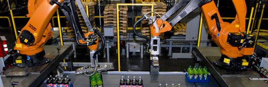
Whether you are packing cartons in cases, pouches in cases, or products in trays, Remtec packing robots can greatly improve the speed and flexibility of you packaging operation. But the robot is only part of the story.

All of Remtec’s packing robots feature highly reliable Lantech case erectors and sealers, which are available in a wide range of tape-seal and glue-seal configurations. In addition, Remtec’s case handling conveyors and flap management systems are designed for maximum reliability and adjustability over a wide range of SKU’s.

All of Remtec’s robotic packing Systems are equipped with standard Allen-Bradley controllers, which eliminate the need for robot programming expertise on the packaging floor. A simple touch screen operator interface is provided so that the system can be operated without specialized training.

Packing Robot System features matched to your needs:

• Turn-key system design
• Conveyors included
• Carton erectors and sealers

picking robot system solutions:

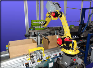
• Case packing of cartons – Remtec’s packing robots are capable of packing individual items or entire product layers at rates up to 25 cases per minute. 

                    

                           Robotic Automation 

According to International Federation of Robotics estimates, there are over 1 million industrial robots in operation today. The majority of industrial robots are deployed in the automotive industry, which was the first industry to adopt robots for production. Remtec Corporation was there in the early growth days of the robotic industry and continues to be a leading innovator in robotic automation.

• Robotic Palletizing
• Automated Packaging
• Automated Material Handling

Today, robotic automation is widely applied across a range of industries. Taken together, packaging and material handling applications represent the largest area of opportunity for realizing the benefits that industrial robots offer, including:

• Reduction in unskilled labor costs
• Safety and elimination of labor-related injuries
• Improved capital allocation through multi-shift operations
• Enhanced production speed and accuracy
• Flexibility and ease of product changeover

An investment in robotic automation offers attractive return on investment because industrial robots can be redeployed many times over an estimated service life of 10-12 years. 

Robotic Palletizing

(877) 759-8151

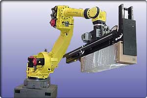
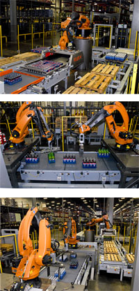
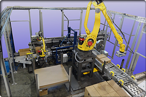The potentially labor intensive process of industrial palletizing, including loading and unloading parts, boxes or other items, is ideally suited to robotic palletizing automation. Robotic palletizing allows a wide range of repetitive labor processes to be performed automatically.

Robotic palletizing has enhanced productivity in many industries including food processing, consumer goods manufacturing, and durable goods manufacturing.  Various end-of-arm-tooling technologies offer flexibility in a variety of palletizing operations.

• Case Palletizing
• Depalletizing 

Remtec’s robotic palletizers provide significant benefits in flexibility and uptime compared to traditional dedicated equipment. Whether you need a low-cost, single-line system that can be set up within a few hours, or a more complex solution with multiple infeeds and outfeeds, Remtec has pre-engineered robotic solutions ready to go. And with Remtec’s simple touchscreen controls interface, SKU setup and changeover is greatly reduced. Remtec offers solutions for:

• Palletizing cases, bags, bundles, and containers
• Palletizing of components or Work-in-Process Inventory
• Depalletizing cases, carton flats, or components 
• Mixed / Rainbow load palletizing

Automated Packaging

(877) 759-8151

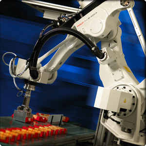In the past, automated packaging was accomplished by relatively inflexible, special purpose machines.  Recently, rapid advances in robot technology offer substantial benefits in higher-rate handling applications such as case packing, tray packing, and kitting.

Robot cycle rates above 100 picks per minute are now common, and integrated vision capability improves product changeover time and reduces system cost. Robotic automated packaging has increased productivity in a wide range of industries including food processing, manufacturing, and consumer goods.  Custom engineered robotic systems offer flexibility in a variety of packaging operations.

• Picking Robots
• Packing Robots
• Kitting Robots

Remtec’s automated packaging robots can significantly improve the efficiency of your upstream packaging operations. Robot systems are highly flexible, with demonstrated abilities in secondary packaging applications such as:

• Packing Robots (case packing, tray packing)
• High speed picking and bag-in-box or pouch-in-box applications
• Kitting and creation of product assortments 

Automated Material Handling

(877) 759-8151

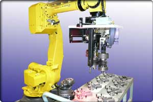In addition to secondary packaging and end of line processes such as packing and palletizing, Remtec has many years of experience in the application of robots to upstream automated material handling Processes. Typical applications include:

• Tending of machine tools, casting machinery, and injection molding machinery
• Product assembly
• Product inspection and gauging
• Buffering and storage/retrieval of in-process inventory

As with all of Remtec’s robotic systems, each automated material handling system is designed for maximum flexibility and ease of use.

• Machine Tool Tending
• Part Handling and Inspection
• Robotic Assembly 

About Packaging Robotics

About Packaging Robotics is dedicated to providing customized solutions to all your package-handling needs.

Since 1981, About Packaging Robotics has been committed to producing high quality, yet affordable robotic package handling systems. Our products are engineered to open, fill, transport, seal, code and label as variety of pre-made pouches and bags. About Packaging Robotics' fine line of packaging and systems for on demand product identification are currently used in the medical, industrial and food industries, with a product line that is efficient and reliable.

Our systems fill the gap between operator-dependent, high-maintenance-personnel-cost; Form-Fill and Seal machines and costly manual package handling.

About Packaging Robotics is dedicated to providing customized solutions to all your package-handling needs. An experienced staff of engineers and technicians comprise the cornerstone of our company. Custom Engineering ensures operational dependability and system integration.

About Packaging Robotics cleanroom compatible systems are designed to handle premade pouches, bags, and flat media. We provide affordable miniature, PLC controlled, Robotic Processing systems to open, fill and seal pouches with only minutes for pouch size changeover. Our systems provide user friendly control systems for the unskilled machine operator and reduce your employee exposure to carpal tunnel syndrome. We include FDA validation and calibration protocols and firmware for the technician and Quality Assurance Department.

Automation and Robotics can lower production costs, stabilize daily output, and enhance consistency and quality of your packages. Our products can free employees from performing simple tasks and utilize their skills in more cost-effective ways to IMPROVE YOUR PROFITS.

Robotics

We produce high quality, yet affordable robotic package handling systems. Our products are engineered to open, fill, transport, seal, code and label as variety of pre-made pouches and bags.

Robotic Palletizing

---

Palletizing refers to the operation of loading an object such as a corrugated carton on a pallet or a similar device in a defined pattern. Depalletizing refers to the operation of unloading the loaded object in the reverse pattern.

Many factories and plants today have automated their application with a palletizing robot solution of some kind. Robotic palletizing technology increases productivity and profitability while allowing for more flexibility to run products for longer periods of time.

A robot control system with a built-in palletizing function makes it possible to load and unload an object without spending a lot of time on teaching. Robotic work cells can be integrated towards any project. With current advancements in end of arm tooling (EOAT), robot palletizing work cells have been introduced to many factory floors.

In Order Fulfillment, there a few robotic solutions that are really revolutionizing the material handling world. These include Layer Forming and Inline Palletizing, Layer Depalletizing and Palletizing, and Mixed Case Palletizing, each have specific benefits that can truly improve a client’s operations with marked productivity, flexibility, and reliability.

Types of Robotic Palletizing Solutions
Inline Palletizing
Layer Depalletizing & Palletizing
Mixed Case Palletizing
Layer Palletizing in the Freezer

---

Types of Robotic Solutions - Inline Palletizing

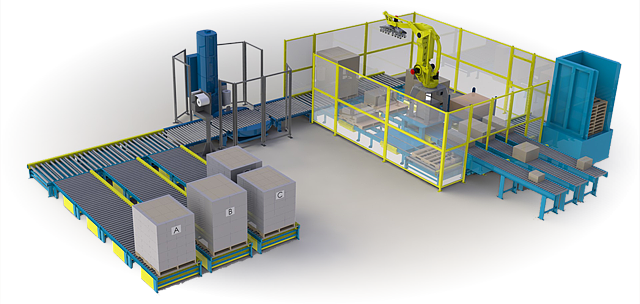
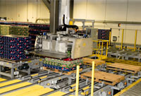
In the past decade, the automated end of line palletizing of same package types has become proven technology. The economic justification of a palletizing system is mainly driven by the achievable throughput (cases per hour), the system availability, the required floor space and the utilization rate of the complete production line. Especially for high throughput demands, e.g. in the beverage industry, robots set new standards in Inline Palletizing. The use of articulated robot enables the implementation of new innovative robot based concepts for the high speed inline palletizing. With form fitting gripper systems, the incoming packages are moved actively and accurately into the correct target positions on a mesh belt conveyor. Hereby the robot motion is synchronized with the conveyor speed thus allowing a reliable layer forming process. Since the packages are gripped actively, the process does not depend on friction and packaging characteristics, which is often a challenge for shrink wrapped items. During the layer forming process, a little gap between the packages is added in order to avoid potential collisions. Once a layer has been completed, a mechanical end stop is lowered and the layer is conveyed to the pick-up position of the layer picking robot. Immediately after the layer has passed the end stop, the end stop is raised again and the next layer can be assembled. The layer picking robot can pull the whole layer with an integrated puller onto the gripper. Inside this gripper the layer is finally centered, thus a compact layer can be placed accurately onto the target pallet. As an option, the layer gripper can add a slip sheet. Depending on the production line speed, the robot-based inline palletizing system can be adapted to its required system performance. E.g., by adding another layer forming robot, the throughput can be doubled.

Seeing the Benefits

• One stop shop solution, from the planning to the world wide after sales support
• High palletizing performance means a high profitability
• A scalable system concept adapted to your production needs
• Small floor space
• High reliability due to layer forming based on form fitted gripping principle
• No package damages to due gentle product handling
• Fast, easy and automated switch over to different package types and dimensions
• Safe and accurate palletizing with layer gripper and integrated centering device
• Universal control architecture
• Robot equipment can easily be re-used in case of production change
• Slip sheet handling can be simply be added to overall system concept (Optional)

---

Types or Robotic Solutions - Layer Depalletizing & Palletizing

Economical automation can only be achieved if the installed equipment is optimally utilized. Transferred into layer picking systems, this implies that you are able to control the process and that the deployed technology can handle the highest percentage of your entire range of products and packaging types.

The variety of different product and packaging types (e.g. corrugated cardboard boxes, shrink wrapped items, open trays or boxes) in a distribution center have little in common, which makes automatic depalletizing and order picking difficult. However, as most package types have at least a flat bottom, universal gripping system has been designed to incorporate a roll-up principle. This enables you to handle layers of products where most other conventional technologies fail.

In this process, two servo driven rubber rollers are pushing against the pallet layer from opposite sides. The packages are thereby lifted up and rolled onto two symmetrical carrier plates. The gripper control software automatically adjusts the contact pressure and height position of the rubber rollers to suit the package weight and dimensions.

The roll-up principle supports a multiple layer pick cycle; thus, the overall picking performance can be significantly increased. The maximum layer number is limited by either the maximum payload weight or the maximum payload height.

Seeing the Benefits

• One stop shop solution, from the planning to the world wide after sales support
• Handling of a wide range of product and packaging types
• High palletizing performance means a high profitability
• No package damages due to gentle product handling and adaptive gripping process
• High system availability and easy operation
• Increased throughput due to multiple layer picking capability (e.g., picking two layers of open trays with cans in one cycle
• Low noise level due to servo drive approach
• Accurate layer placement due to integrated layer centering
• No product drop in case of a power failure
• Safe gripping of layers even with holes and gaps in the pallet pattern
• High flexibility of palletizing line due to the use of robots
• High standardization (reduction of costs)

---

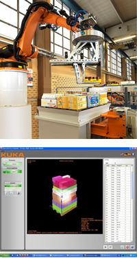
Types of Robotic Solutions - Mixed Case Palletizing

In the past decade, true mixed package type palletizing has become proven technology. The economic justification of a palletizing system is mainly driven by the achievable throughput (cases per hour), the system availability, the required floor space and the utilization rate of the complete production line. As SKU proliferation has escalated, this task has also become very labor intensive as well The demands made on automated order picking in distribution centers grow by the day. Orders, articles, and a wide variety of containers must be picked and palletized, whether on pallets or pushcarts, right on schedule and with a minimum of errors The range of articles and the dimensions and materials of the packaging units are virtually unlimited, be it open or closed trays or beverages wrapped in PET film. In response to these demands, an application module called Pallet-MIX for automated palletizing has been developed. The primary objective was the development of an application module using service, proven jointed-arm robots together with innovative software and gripper technology. A conscious decision was made in favor of a jointed-arm robot with six degrees of freedom, in order to avoid the need for external turning of the packaging unit. This represents a significant advantage over gantry solutions. Performance and reliable palletizing of the packages were the prime criteria, with the aim of achieving high throughput rates.

Seeing the Benefits

• Single-source solution, from the planning to the world wide after sales support
• Wide range of palletizable packing units
• Short cycle times, giving maximum cost-effectiveness
• Gentle handling using a servo gripper
• Minimized number of pallets
• Maximized packing density
• High system flexibility through the use of jointed-arm robots (no additional turning station required)
• High level of standardization (reduction of costs)

---

Types of Robotic Solutions - Layer Palletizing in the Freezer

During the past decades the proportion of deep frozen products in the food market has increased continuously in Europe and in the US. The main advantage for the customer is evident: a long storage life. These products have to be order-picked in a very cold distribution center. Up to now, this process has been done manually resulting in a high fluctuation of the work force.

At this temperature level (-30 °C; -22 °F), not only do the workers have to keep themselves warm, but the technical equipment is adversely affected: Lubricants lose their viscosity, plastics become hard and brittle, microelectronics (controller hardware) and sensors are usually not specified for such temperatures.

One or two companies have taken up these particular challenges and have developed a system for layer-wise order picking that can cope with these harsh environmental conditions. In this solution, source pallets are placed alternately on two in-feeding chain conveyors. The robot depalletizes the required number of layers from the source pallet and transfers them onto the target pallet, which is transported on a third conveyor. The picking sequence is specified by the customer’s order lines and the valid stacking rules; Thus the source pallets have to be supplied in the pre-defined order.

The gripper concept combines vacuum and clamping technology. The deployed components have been carefully selected to ensure a reliable operation in these extreme temperatures. Due to this approach, technology has proven that a wide range of deep frozen products can be handled successfully using standard packages. The servo-driven side clamps are used and moved to the optimum clamping position in relation to the product height. Sensors detect the current height of the top layer and the existence of slip sheets.

Slip sheets are picked with a reduced vacuum level and are transferred onto a slip sheet deposit position or onto the target pallet depending on the customer’s preference. If necessary, the side clamps can also pick up empty pallets. Thus the robot can remove empty pallets from the source conveyors or provide itself a new empty starter pallet onto the target conveyor.

Seeing the Benefits

• One stop shop solution, from the planning to the world wide after sales support
• High palletizing performance means a high profitability
• Distinct reduction on hard physical labor in a harsh environment
• A scalable system concept adaptable to your production needs
• Small floor space
• High system availability
• No package damages to due gentle product handling
• Safe and accurate palletizing with layer gripper and integrated centering device
• Universal control architecture
• Robot equipment can easily be re-used in case of production change
• Handling of slip sheets and empty pallets already integrated into the concept

      

  

Control and Robotic Systems (CRS)

Research in this area covers control and robotic systems technologies and their applications in next-generation industry robots, manufacturing automation, aeronautical and aerospace systems, autonomous vehicles, energy systems, intelligent transportation, medical and healthcare systems.

 

Packaging

KEY INDUSTRY EXPERTISE

• Pick and Place
• Small Electronic Parts Assembly
• Labeling
• Load and Unload
• Marking and Printing
• Scribing
• High-Speed Registration
• Electronic Gearing

The Total Package

Aerotech manufactures motion control systems and components for automated packaging equipment and packaging systems, and is well-versed in applications such as load and unload, marking and printing, labeling, scribing, high-speed registration, electronic gearing and others. We can customize an automated packaging equipment system to meet your needs or you can choose from our wide array of components including gantries, rotary and linear and lift stages, PWM and linear drives, brush and brushless rotary motors and linear motors, and advanced motion controllers. This makes us a complete packaging equipment solution provider, as well as a source for high-performance components for retrofit of existing automated packaging equipment systems.

A Gantry for Every Occasion

Aerotech gantry systems use our own brushless linear servomotors to meet the needs of a variety of gantry customers, from packaging applications to electronic assembly and electronic manufacturing to vision systems and industrial automation. These industrial robots are available in models from low-cost modular linear actuators assembled in a gantry configuration with matching motion control and drives, to sophisticated gantry models with the largest travel, highest speed and highest acceleration available.

Control is Key

Aerotech motion controllers are used in our own positioning systems and in motion control and positioning systems throughout the world. The Automation 3200 multi-axis motion controller is software-based (no PC slots required) and marries a robust, high performance motion engine with vision, PLC, robotics, and I/O in one unified programming environment. The Ensemble™ stand-alone 1-10 axis motion controller is Aerotech's next-generation controller for moderate- to high-performance applications with high-speed communication through 10/100 Base T Ethernet or USB interfaces. The Soloist™ is a single-axis servo controller that combines a power supply, amplifier and position controller in a single package. 

Motion Solutions for your Electronics Manufacturing Applications

With over 45 years of precision motion excellence, Aerotech offers world-class motion solutions for various applications in electronics manufacturing, including laser direct imaging, stencil cutting, micro-electronics assembly, PCB processing, and back-end semiconductor processes including die inspection, dicing, and IC bonding. From high-performance components, to fully-integrated electro-mechanical subsystems, Aerotech has a solution that will suit your needs. Whatever precision motion is required for your specific application, Aerotech can offer a solution optimized for your performance objectives by our engineering team.

Aerotech manufactures many systems for standard industrial environments, but also has competencies in numerous types of systems requiring special environmental and process considerations, including:

• Electrostatic Discharge Protection
• Cleanroom Ready Systems
• Vacuum Ready Systems

In addition to precision mechanics, Aerotech also offers highly advanced software packages to control your motion system. The A3200 Software-Based Controller is among the most powerful motion controllers on the market with unique features and capabilities seamlessly control and coordinate any combination of servo, galvo, and piezo systems. Our A3200 controller has numerous built-in algorithms and features specifically designed for electronics manufacturing applications, including:

• Enhanced Tracking Control: Improves following errors in contouring motion and reduces move and settle time in point-to-point positioning
• Enhanced Throughput Module: Counteracts disturbances caused by outside forces and vibrations
• Command Shaping: Improves settling time and dynamic performance by eliminating errors caused by system resonances (included in Dynamic Controls Toolbox)
• EasyTune: Avoid the hassles of tuning a mechatronic motion system; automatically tune your system in minutes with just a single click of a button

Related Industry Solution PagesMicro-Electronics Assembly
Printed Electronics/Dispensing
Via Drilling
Wafer Dicing

Gold Standard Gantries

Aerotech's industrial robots are available in models from low-cost, modular, linear actuators assembled in a gantry configuration, to sophisticated gantry models with the largest travel, highest speed and highest acceleration available. Aerotech’s world-class gantries are used in a wide array of electronics manufacturing applications around the world, including pick-and-place, printing circuits, drilling vias in PCBs, manufacturing laser-cut stencils, and many more high-precision processes. Aerotech's experience in brushless linear motor design, motion controllers, and drives enables us to offer a complete gantry solution that perfectly fits your gantry application.

Piezo Nanopositioners

Aerotech’s QNP™ series and QNP_HD series of piezo nanopositioning stages offer sub-nanometer-level performance in a compact, high-stiffness package. A variety of travel (100 µm to 600 µm) and feedback options make this the ideal solution for applications ranging from microscopy to optics alignment. For electronics manufacturing applications that require sub-micron levels of motion control, piezo stages can be the perfect solution. If your system requires both piezo stages and servo stages, our A3200 controller has the unprecedented capability of controlling and coordinating motion between both axes, despite their fundamental functional differences. 

++++++++++++++++++++++++++++++++++++++++++++++++++++++++

                       PACKAGING  AND WRAP  WITH ELECTRONICS ROBO

++++++++++++++++++++++++++++++++++++++++++++++++++++++++