
Math Center
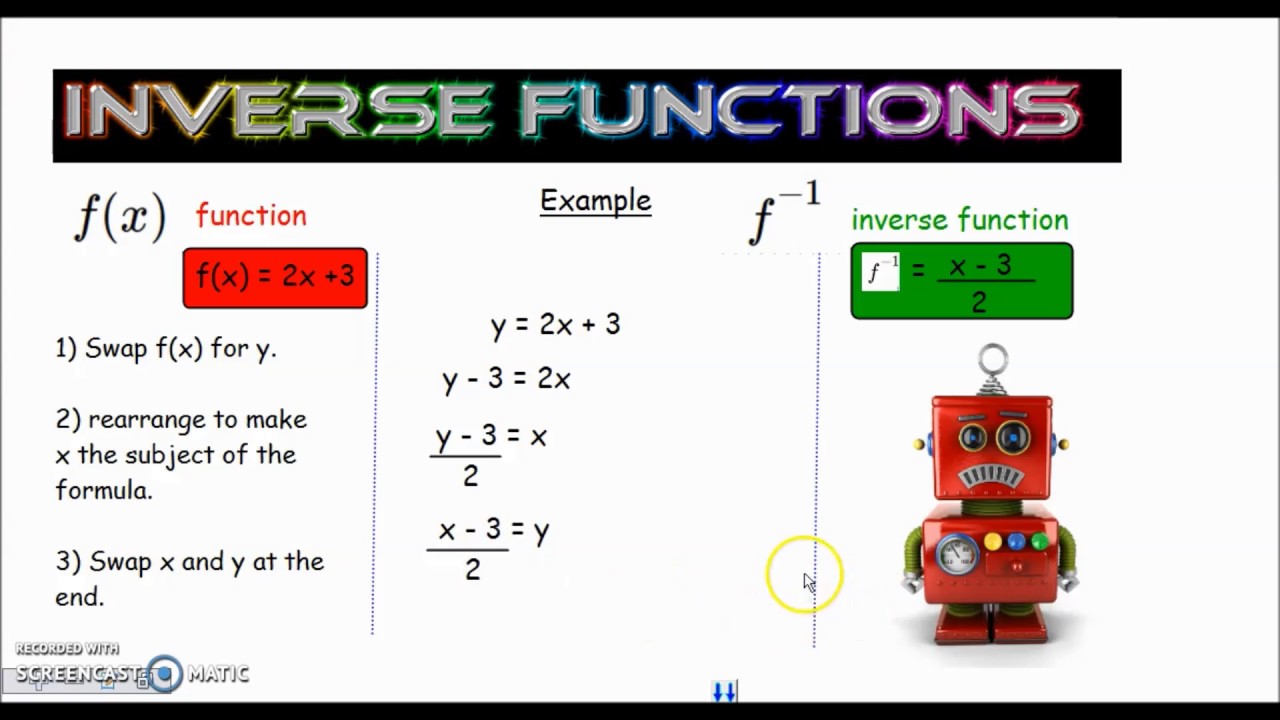
Inverse Functions
Two functions are inverses of one another if they "undo each other" in the following sense: if the output of one is used as input to the other, they leave the original input unchanged.
To be precise, two functions and are inverses of each other if and only if for every value of in the domain of and for every value of in the domain of .
Graphs of Inverse Functions

The Horizontal Line Test
Not every function is invertible. Fortunately, we can tell which functions are invertible from those that are not by a quick examination of their graphs
Inverse Operations and Functions
An operation we might do with a glove is put on. Another operation that could be done is take off. If we start with a bare hand:
If we start with a glove on:

The operations put on and take off undo each other. If we do one operation then the other, we end up where we started. Put on is the inverse operation to take off. Take off is the inverse operation of put on. Such operations form an operation-inverse operation pair.
The same is true in mathematics. Most operations have an inverse operation. Starting with the simplest operations:
Let's think about exponents. We can get from a number to that number to the power of 2 by squaring the number. To get back to the original number we need to take the square root.
Sometimes an operation is its own inverse. Take a bus is an example.

XXX . XXX All About XOR
Boolean operators are the bedrock of computer logic. Michael Lewin investigates a common one and shows there’s more to it than meets the eye.
You probably already know what XOR is, but let’s take a moment to formalise it. XOR is one of the sixteen possible binary operations on Boolean operands. That means that it takes 2 inputs (it’s binary) and produces one output (it’s an operation), and the inputs and outputs may only take the values of TRUE or FALSE (it’s Boolean) – see Figure 1. We can (and will) interchangeably consider these values as being 1 or 0 respectively, and that is why XOR is typically represented by the symbol ⊕: it is equivalent to the addition operation on the integers modulo 2 (i.e. we wrap around so that 1 + 1 = 0)1 [SurreyUni]. I will use this symbol throughout, except in code examples where I will use the C operator
Certain Boolean operations are analogous to set operations (see Figure 2): AND is analogous to intersection, OR is analogous to union, and XOR is analogous to set difference. This is not just a nice coincidence; mathematically it is known as an isomorphism2 and it provides us with a very neat way to visualise and reason about such operations.
The last, and most powerful, interpretation of XOR is in terms of parity, i.e. whether something is odd or even. For any n bits, A1 ⊕ A2 ⊕ … ⊕ An = 1 if and only if the number of 1s is odd. This can be proved quite easily by induction and use of associativity. It is the crucial observation that leads to many of the properties that follow, including error detection, data protection and adding.
Toggling in this way is very similar to the concept of a flip-flop in electronics: a ‘circuit that has two stable states and can be used to store state information’ [Wikipedia-1].
Perhaps there is some retribution for this much maligned idea, however. This is more than just a devious trick when we consider it in the context of assembly language. In fact XOR’ing a register with itself is the fastest way for the compiler to zero the register.
Note that the nodes at either end store the address of their neighbours. This is consistent because conceptually we have XOR’ed that address with 0. Then the code to traverse the list looks like Listing 1, which was adapted from Stackoverflow [Stackoverflow].
This uses the same idea as before, that one state is the key to getting at the other. If we know the address of any consecutive pair of nodes, we can derive the address of their neighbours. In particular, by starting from one end we can traverse the list in its entirety. A nice feature of this function is that this same code can be used to traverse either forwards or backwards. One important caveat is that it cannot be used in conjunction with garbage collection, since by obfuscating the nodes’ addresses in this way the nodes would get marked as unreachable and so could be garbage collected prematurely.
The choice of key here is crucial to the strength of the encryption. If it is short, then the code could easily be cracked using the centuries-old technique of frequency analysis. As an extreme example, if the key is just 1 byte then all we have is a substitution cipher that consistently maps each letter of the alphabet to another one. However, if the key is longer than the message, and generated using a ‘truly random’ hardware random number generator, then the code is unbreakable [Wikipedia-3]. In practice, this ‘truly random’ key could be of fixed length, say 128 bits, and used to define a linear feedback shift register that creates a pseudorandom sequence of arbitrary length known as a keystream. This is known as a stream cipher, and in a real-worl situation this would also be combined with a secure hash function such as md5 or SHA-1.
Another type of cipher is the block cipher which operates on the message in blocks of fixed size with an unvarying transformation. An example of XOR in this type of encryption is the International Data Encryption Algorithm (IDEA) [Wikipedia-4].
The best-known encryption method is the RSA algorithm. Even when the above algorithm is made unbreakable, it has one crucial disadvantage: it is not a public key system like RSA. Using RSA, I can publish the key others need to send me encrypted messages, but keep secret my private key used to decrypt them. On the other hand, in XOR encryption the same key is used to encrypt and decrypt (again we see an example of toggling). Before you can send me encrypted messages I must find a way to secretly tell you the key to use. If an adversary intercepts that attempt, my code is compromised because they will be able to decrypt all the messages you send me.
Checksums and cyclic redundancy checks (CRC) extend the concept to longer check values and reducing the likelihood of collisions and are widely used. It’s important to note that such checks are error-detecting but not error-correcting: we can tell that an error has occurred, but we don’t know where it occurred and so can’t recover the original message. Examples of error-correcting codes that also rely on XOR are BCH and Reed-Solomon [Wikipedia-5][IEEEXplore].
A* = A1 ⊕ A2 ⊕ … ⊕ An
This introduces redundancy: if a failure occurs on one drive, say A1, we can restore it from the others since:
This is the same reasoning used to explain toggling earlier, but applied to n inputs rather than just 2.
In the (highly unlikely) event that 2 drives fail simultaneously, the above would not be applicable so there would be no way to recover the data.
Computers are built from logic gates, which are in turn built from transistors. A transistor is simply a switch that can be turned on or off using an electrical signal (as opposed to a mechanical switch that requires a human being to operate it). So for example, the AND gate can be built from two transistors in series, since both switches must be closed to allow current to flow, whereas the OR gate can be built from two transistors in parallel, since closing either switch will allow the current to flow.
Most binary logical operations can be constructed from two or fewer transistors; of all 16 possible operations, the only exception is XOR (and its complement, XNOR, which shares its properties). Until recently, the simplest known way to construct XOR required six transistors [Hindawi]: the simplest way to see this is in the diagram below, which comprises three gates, each of which requires two transistors. In 2000, Bui et al came up with a design using only four transistors [Bui00] – see Figure 5.
A new mortgage application might be evaluated using this model to determine whether the applicant is likely to default.
Not all problems are neatly separable in this way. That means we either need more than one boundary line, or we need to apply some kind of non-linear transformation into a new space in which it is linearly separable: this is how machine learning techniques such as neural networks and support vector machines work. The transformation process might be computationally expensive or completely unachievable. For example, the most commonly used and rigorously understood type of neural network is the multi-layer perceptron. With a single layer it is only capable of classifying linearly separable problems. By adding a second layer it can transform the problem space into a new space in which the data is linearly separable, but there’s no guarantee on how long it may take to converge to a solution.
So where does XOR come into all this? Let’s picture our binary Boolean operations as classification tasks, i.e. we want to classify our four possible inputs into the class that outputs TRUE and the class that outputs FALSE. Of all the 16 possible binary Boolean operations, XOR is the only one (with its complement, XNOR) that is not linearly separable with a single boundary line: two lines are required, as the diagram in Figure 7 demonstrates.
Now of course we want to do a lot more than just add two bits: just like you learnt in primary school, we need to carry the ‘carry bit’ along because it will play a part in the calculation of the higher order bits. For that we need to augment what we have into a full adder. We’ve added a third input that enables us to pass in a carry bit from some other adder. We begin with a half adder to add our two input bits. Then we need another half adder to add the result to the input carry bit. Finally we use an OR gate to combine the carry bits output by these two half adders into our overall output carry bit. (If you’re not convinced of this last step, try drawing the truth table.) This structure is represented in Figure 9.
Now we are able to chain as many of these adders together as we wish in order to add numbers of any size. The diagram below shows an 8-bit adder array, with the carry bits being passed along from one position to the next. Everything in electronics is modular, so if you want to add 32-bit numbers you could buy four of these components and connect them together (see Figure 10).
If you are interested in learning more about the conceptual building blocks of a modern computer, Charles Petzold’s book Code comes highly recommended.
An algebraic structure is simply a mathematical object (S, ~) comprising a set S and a binary operation ~ defined on the set.
A group is an algebraic structure such that the following 4 properties hold:
Two groups are said to be isomorphic if there is a one-to-one mapping between the elements of the sets that preserves the operation. I won’t write that out formally (it’s easy enough to look up) or prove the isomorphisms below (let’s call that an exercise for the reader). Instead I will just define them and state that they are isomorphisms.
The group ({T, F}N, XOR) is isomorphic to the group ({0, 1}N, +) of addition modulo 2 over the set of vectors whose elements are integers mod 2. The isomorphism simply maps T to 1 and F to 0.
The group ({T, F}N, XOR) is also isomorphic to the group (P(S), Δ) of symmetric difference Δ over the power set of N elements3: the isomorphism maps T to ‘included in the set’ and F to ‘excluded from the set’ for each of the N entries of the Boolean vector.
Let’s take things one step further by considering a new algebraic structure called a ring. A ring (S,+, ×) comprises a set S and a pair of binary operations + and × such that S is an Abelian group under + and a semigroup4 under ×. Also × is distributive over +. The symbols + and × are chosen deliberately because these properties mean that the two operations behave like addition and multiplication.
We’ve already seen that XOR is an Abelian group over the set of Boolean vectors, so it can perform the role of the + operation in a ring. It turns out that AND fulfils the role of the * operation. Furthermore we can extend the isomorphisms above by mapping AND to multiplication modulo 2 and set intersection respectively. Thus we have defined three isomorphic rings in the spaces of Boolean algebra, modulo arithmetic and set theory.
^ to represent XOR.
| ||||||||||||||||||
| Figure 1 | ||||||||||||||||||
 |
 |
 |
| Figure 2 |
Important properties of XOR
There are 4 very important properties of XOR that we will be making use of. These are formal mathematical terms but actually the concepts are very simple.- Commutative: A ⊕ B = B ⊕ A This is clear from the definition of XOR: it doesn’t matter which way round you order the two inputs.
- Associative: A ⊕ ( B ⊕ C ) = ( A ⊕ B ) ⊕ C This means that XOR operations can be chained together and the order doesn’t matter. If you aren’t convinced of the truth of this statement, try drawing the truth tables.
- Identity element: A ⊕ 0 = A This means that any value XOR’d with zero is left unchanged.
- Self-inverse: A ⊕ A = 0 This means that any value XOR’d with itself gives zero.
Interpretations
We can interpret the action of XOR in a number of different ways, and this helps to shed light on its properties. The most obvious way to interpret it is as its name suggests, ‘exclusive OR’: A ⊕ B is true if and only if precisely one of A and B is true. Another way to think of it is as identifying difference in a pair of bytes: A ⊕ B = ‘the bits where they differ’. This interpretation makes it obvious that A ⊕ A = 0 (byte A does not differ from itself in any bit) and A ⊕ 0 = A (byte A differs from 0 precisely in the bit positions that equal 1) and is also useful when thinking about toggling and encryption later on.The last, and most powerful, interpretation of XOR is in terms of parity, i.e. whether something is odd or even. For any n bits, A1 ⊕ A2 ⊕ … ⊕ An = 1 if and only if the number of 1s is odd. This can be proved quite easily by induction and use of associativity. It is the crucial observation that leads to many of the properties that follow, including error detection, data protection and adding.
Toggling
Armed with these ideas, we are ready to explore some applications of XOR. Consider the following simple code snippet: for (int n=x; true; n ^= (x ^ y))
printf("%d ", n);
This will toggle between two values x and y, alternately printing one and then the other. How does it work? Essentially the combined value x ^ y ‘remembers’ both states, and one state is the key to getting at the other. To prove that this is the case we will use all of the properties covered earlier:| B ⊕ ( A ⊕ B ) | (commutative ) |
| = B ⊕ ( B ⊕ A ) | (associative) |
| = (B ⊕ B) ⊕ A | (self-inverse) |
| = 0 ⊕ A | (identity element) |
| = A |
Save yourself a register
Toggling is all very well, but it’s probably not that useful in practice. Here’s a function that is more useful. If you haven’t encountered it before, see if you can guess what it does. void s(int& a, int& b)
{
a = a ^ b;
b = a ^ b;
a = a ^ b;
}
Did you work it out? It’s certainly not obvious, and the below equivalent function is even more esoteric: void s(int& a, int& b)
{
a ^= b ^= a ^= b;
}
It’s an old trick that inspires equal measures of admiration and vilification. In fact there is a whole repository of interview questions whose name is inspired by this wily puzzle: http://xorswap.com/. That’s right, it’s a function to swap two variables in place without having to use a temporary variable. Analysing the first version: the first line creates the XOR’d value. The second line comprises an expression that evaluates to a and stores it in b, just as the toggling example did. The third line comprises an expression that evaluates to b and stores it in a. And we’re done! Except there’s a bug: what happens if we call s(myVal, myVal)? This is an example of aliasing, where two arguments to a function share the same location in memory, so altering one will affect the other. The outcome is that myVal == 0 which is certainly not the semantics we expect from a swap function!Perhaps there is some retribution for this much maligned idea, however. This is more than just a devious trick when we consider it in the context of assembly language. In fact XOR’ing a register with itself is the fastest way for the compiler to zero the register.
Doubly linked list
A node in a singly linked list contains a value and a pointer to the next node. A node in a doubly linked list contains the same, plus a pointer to the previous node. But in fact it’s possible to do away with that extra storage requirement. Instead of storing either pointer directly, suppose we store the XOR’d value of the previous and next pointers [Wikipedia-2] – see Figure 3. |
| Figure 3 |
// traverse the list given either the head or
// the tail
void traverse( Node *endPoint )
{
  Node* prev = endPoint;
  Node* cur = endPoint;

  while ( cur )
  // loop until we reach a null pointer
  {
    printf( "value = %d\n", cur->value);
    if ( cur == prev )

// only true on first iteration
      cur = cur->prevXorNext;
      // move to next node in the list
    else
    {
      Node* temp = cur;
      cur = (Node*)((uintptr_t)prev
         ^ (uintptr_t)cur->prevXorNext);
      // move to next node in the list
      prev = temp;
    }
  }
}
|
| Listing 1 |
Pseudorandom number generator
XOR can also be used to generate pseudorandom numbers in hardware. A pseudorandom number generator (whether in hardware or software e.g. std::rand() ) is not truly random; rather it generates a deterministic sequence of numbers that appears random in the sense that there is no obvious pattern to it. This can be achieved very fast in hardware using a linear feedback shift register. To generate the next number in the sequence, XOR the highest 2 bits together and put the result into the lowest bit, shifting all the other bits up by one. This is a simple algorithm but more complex ones can be constructed using more XOR gates as a function of more than 2 of the lowest bits [Yikes]. By choosing the architecture carefully, one can construct it so that it passes through all possible states before returning to the start of the cycle again (Figure 4). |
| Figure 4 |
Encryption
The essence of encryption is to apply some key to an input message in order to output a new message. The encryption is only useful if it is very hard to reverse the process. We can achieve this by applying our key over the message using XOR (see Listing 2).string EncryptDecrypt(string inputMsg,string key)
{
string outputMsg(inputMsg);
short unsigned int keyLength = key.length();
short unsigned int strLength =
inputMsg.length();
for(int v=0, k=0;v<strLength;++v)
{
outputMsg[v] = inputMsg[v]^key[k];
++k;
k = k % keyLength;
}
return outputMsg;
}
|
| Listing 2 |
Another type of cipher is the block cipher which operates on the message in blocks of fixed size with an unvarying transformation. An example of XOR in this type of encryption is the International Data Encryption Algorithm (IDEA) [Wikipedia-4].
The best-known encryption method is the RSA algorithm. Even when the above algorithm is made unbreakable, it has one crucial disadvantage: it is not a public key system like RSA. Using RSA, I can publish the key others need to send me encrypted messages, but keep secret my private key used to decrypt them. On the other hand, in XOR encryption the same key is used to encrypt and decrypt (again we see an example of toggling). Before you can send me encrypted messages I must find a way to secretly tell you the key to use. If an adversary intercepts that attempt, my code is compromised because they will be able to decrypt all the messages you send me.
Error detection
Now we will see the first application of XOR with respect to parity. There are many ways to defend against data corruption when sending digital information. One of the simplest is to use XOR to combine all the bits together into a single parity bit which gets appended to the end of the message. By comparing the received parity bit with the calculated one, we can reliably determine when a single bit has been corrupted (or indeed any odd number of bits). But if 2 bits have been corrupted (or indeed any even number of bits) this check will not help us.Checksums and cyclic redundancy checks (CRC) extend the concept to longer check values and reducing the likelihood of collisions and are widely used. It’s important to note that such checks are error-detecting but not error-correcting: we can tell that an error has occurred, but we don’t know where it occurred and so can’t recover the original message. Examples of error-correcting codes that also rely on XOR are BCH and Reed-Solomon [Wikipedia-5][IEEEXplore].
RAID data protection
The next application of XOR’s parity property is RAID (Redundant Arrays of Inexpensive Disks) [Mainz] [DataClinic]. It was invented in the 1980s as a way to recover from hard drive corruption. If we have n hard drives, we can create an additional one which contains the XOR value of all the others:A* = A1 ⊕ A2 ⊕ … ⊕ An
This introduces redundancy: if a failure occurs on one drive, say A1, we can restore it from the others since:
| A2 ⊕ … ⊕ An ⊕ A* | |
| = A2 ⊕ … ⊕ An ⊕ (A1 ⊕ A2 ⊕ … ⊕ An) | (definition of A*) |
| = A1 ⊕ (A2 ⊕ A2) ⊕… ⊕ (An ⊕ An) | (commutative and associative: rearrange terms) |
| = A1 ⊕ 0 ⊕… ⊕ 0 | (self-inverse) |
| = A1 | (identity element) |
In the (highly unlikely) event that 2 drives fail simultaneously, the above would not be applicable so there would be no way to recover the data.
Building blocks of XOR
Let’s take a moment to consider the fundamentals of digital computing, and we will see that XOR holds a special place amongst the binary logical operations.Computers are built from logic gates, which are in turn built from transistors. A transistor is simply a switch that can be turned on or off using an electrical signal (as opposed to a mechanical switch that requires a human being to operate it). So for example, the AND gate can be built from two transistors in series, since both switches must be closed to allow current to flow, whereas the OR gate can be built from two transistors in parallel, since closing either switch will allow the current to flow.
Most binary logical operations can be constructed from two or fewer transistors; of all 16 possible operations, the only exception is XOR (and its complement, XNOR, which shares its properties). Until recently, the simplest known way to construct XOR required six transistors [Hindawi]: the simplest way to see this is in the diagram below, which comprises three gates, each of which requires two transistors. In 2000, Bui et al came up with a design using only four transistors [Bui00] – see Figure 5.
 |
| Figure 5 |
Linear separability
Another way in which XOR stands apart from other such operations is to do with linear separability. This is a concept from Artificial Intelligence relating to classification tasks. Suppose we have a set of data that fall into two categories. Our task is to define a single boundary line (or, extending the notion to higher dimensions, a hyperplane) that neatly partitions the data into its two categories. This is very useful because it gives us the predictive power required to correctly classify new unseen examples. For example, we might want to identify whether or not someone will default on their mortgage payments using only two clues: their annual income and the size of their property. Figure 6 is a hypothetical example of how this might look. |
| Figure 6 |
Not all problems are neatly separable in this way. That means we either need more than one boundary line, or we need to apply some kind of non-linear transformation into a new space in which it is linearly separable: this is how machine learning techniques such as neural networks and support vector machines work. The transformation process might be computationally expensive or completely unachievable. For example, the most commonly used and rigorously understood type of neural network is the multi-layer perceptron. With a single layer it is only capable of classifying linearly separable problems. By adding a second layer it can transform the problem space into a new space in which the data is linearly separable, but there’s no guarantee on how long it may take to converge to a solution.
So where does XOR come into all this? Let’s picture our binary Boolean operations as classification tasks, i.e. we want to classify our four possible inputs into the class that outputs TRUE and the class that outputs FALSE. Of all the 16 possible binary Boolean operations, XOR is the only one (with its complement, XNOR) that is not linearly separable with a single boundary line: two lines are required, as the diagram in Figure 7 demonstrates.
 |
 |
| Figure 7 |
Inside your ALU
XOR also plays a key role inside your processor’s arithmetic logic unit (ALU). We’ve already seen that it is analogous to addition modulo 2, and in fact that is exactly how your processor calculates addition too. Suppose first of all that you just want to add 2 bits together, so the output is a number between 0 and 2. We’ll need two bits to represent such a number. The lower bit can be calculated by XOR’ing the inputs. The upper bit (referred to as the ‘carry bit’) can be calculated with an AND gate because it only equals 1 when both inputs equal 1. So with just these two logic gates, we have a module that can add a pair of bits, giving a 2-bit output. This structure is called a half adder and is depicted in Figure 8. |
| Figure 8 |
 |
| Figure 9 |
 |
| Figure 10 |
More detail on the Group Theory
For those comfortable with the mathematics, here is a bit more detail of how XOR fits into group theory.An algebraic structure is simply a mathematical object (S, ~) comprising a set S and a binary operation ~ defined on the set.
A group is an algebraic structure such that the following 4 properties hold:
- ~ is closed over X, i.e. the outcome of performing ~ is always an element of X
- ~ is associative
- An identity element e exists that, when combined with any other element of X, leaves it unchanged
- Every element in X has some inverse that, when combined with it, gives the identity element
std::vector, which has variable length.)We have already seen that XOR is associative, that the vector (F, … F) is the identity element and that every element has itself as an inverse. It’s easy to see that it is also closed over the set. Hence (S, XOR) is a group. In fact it is an Abelian group because we showed above that XOR is also commutative.Two groups are said to be isomorphic if there is a one-to-one mapping between the elements of the sets that preserves the operation. I won’t write that out formally (it’s easy enough to look up) or prove the isomorphisms below (let’s call that an exercise for the reader). Instead I will just define them and state that they are isomorphisms.
The group ({T, F}N, XOR) is isomorphic to the group ({0, 1}N, +) of addition modulo 2 over the set of vectors whose elements are integers mod 2. The isomorphism simply maps T to 1 and F to 0.
The group ({T, F}N, XOR) is also isomorphic to the group (P(S), Δ) of symmetric difference Δ over the power set of N elements3: the isomorphism maps T to ‘included in the set’ and F to ‘excluded from the set’ for each of the N entries of the Boolean vector.
Let’s take things one step further by considering a new algebraic structure called a ring. A ring (S,+, ×) comprises a set S and a pair of binary operations + and × such that S is an Abelian group under + and a semigroup4 under ×. Also × is distributive over +. The symbols + and × are chosen deliberately because these properties mean that the two operations behave like addition and multiplication.
We’ve already seen that XOR is an Abelian group over the set of Boolean vectors, so it can perform the role of the + operation in a ring. It turns out that AND fulfils the role of the * operation. Furthermore we can extend the isomorphisms above by mapping AND to multiplication modulo 2 and set intersection respectively. Thus we have defined three isomorphic rings in the spaces of Boolean algebra, modulo arithmetic and set theory.
- Formally, the actions of XOR and AND on {0,1}N form a ring that is isomorphic to the actions of set difference and union on sets. For more details see the appendix.
- The power set means the set of all possible subsets, i.e. this is the set of all sets containing up to N elements.
- A semigroup is a group without the requirement that every element has an inverse.
XXX . XXX 4%zero FINDING INVERSE FUNCTIONS
(switch input/output names method)
(switch input/output names method)
In this lesson and the previous one, we look at two common techniques for getting a formula for .
This author strongly prefers the mapping diagram method of the previous lesson,
because it emphasizes the fact that does something, and undoes it.
That method, however, only works when the formula for contains exactly one appearance of the input variable.
The method discussed in this lesson, dubbed the ‘Switch Input/Output Names’ method, is more widely applicable.
However, it tends to be quite mechanical—if you're not careful, you can just ‘go through the motions’ and forget the underlying idea!
Input/Output Roles for a Function and its Inverse are Switched
The input/output roles for a function and its inverse are switched—the inputs to one are the outputs from the other.If a function takes to , then takes back to .
In other words, if , then .
This is the reason we ‘switch the names’ in the method discussed next!
‘SWITCH INPUT/OUTPUT NAMES’ METHOD FOR FINDING
- replace the function notation
by the variable
;
this is the equation - switch
and
;
this new equation is - solve this new equation for
;
this yields the equation - switch to function notation by replacing by
Example: the ‘Switch Input/Output Names’ Method
In this example, the ‘switch input/output names’ method for finding the inverse is applied to the function .Note that the mapping diagram method cannot be used for this function,
since it contains two appearances of the input variable .
- Start with
.
Replace the function notation with , giving:
In this equation, is the input to and is the output from . - Switch the names
and
to get:
Now, represents an output from , which is an input to .
Now, represents an input to , which is output from . - Solve this new equation for
. This is the part that requires some work:
you must get all the variables ‘upstairs’, on the same side of the equation start by clearing fractions multiply out rearrange: get all terms containing on the same side; move other terms to the other side factor out solve for - Switch to function notation, by renaming
as
:
Done!
Checking: Great Practice with Function Composition
It's fantastic practice to check that and .Along the way you end up with ‘complex fractions’—fractions within fractions.
Note the multiply-by-one technique used to turn these complex fractions into ‘simple‘ fractions!
Push switch
- A push to make switch allows electricity to flow between its two contacts when held in. When the button is released, the circuit is broken. This type of switch is also known as a Normally Open (NO) Switch. (Examples: doorbell, computer case power switch, calculator buttons, individual keys on a keyboard)

- A push to break switch does the opposite, i.e. when the button is not pressed, electricity can flow, but when it is pressed the circuit is broken. This type of switch is also known as a Normally Closed (NC) Switch. (Examples: Fridge Light Switch, Alarm Switches in Fail-Safe circuits)
Many Push switches are designed to function as both push to make and push to break switches. For these switches, the wiring of the switch determines whether the switch functions as a push to make or as a push to break switch.


Inverse of a fuzzy matrix of fuzzy
The aim of this paper is to extend the concept of inverse of a matrix with fuzzy numbers as its elements, which may be used to model uncertain and imprecise aspects of real-world problems. We pursue two main ideas based on employing real scenarios and arithmetic operators. In each case, exact and inexact strategies are provided. In the first idea, we give some necessary and sufficient conditions for invertibility of fuzzy matrices based on regularity of their scenarios. And then Zadeh's extension principle and interpolation on Rohn's approach for inverting interval matrices are followed to compute fuzzy inverse. In the second idea, Dubois and Prade's arithmetic operators will be employed for the same purpose. But with respect to the inherent difficulties which are derived from the positivity restriction on spreads of fuzzy numbers, the concept of ϵ-inverse of a fuzzy matrix and its relaxation are generalized and some useful theorems will be revealed. Finally fuzzifying the defuzzified version of the original problem for introducing fuzzy inverse, which can be followed by each idea, will be presented .
How do you inverse the function of a LDR (Light Dependent Resistor) ....?

the transistor as a switch. When the voltage across BE goes above a certain voltage it allows current to flow between C and E, powering the LED. The potentiometer allows you to vary the ratio of the potential divider and hence the level of light at which the LED turns on.
the transistor needs minimum 0.7volts to function ..
so we use it as a switch ...
The LDR on BRIGHTNESS.. LOWERS the resistance .. which in turn will LOWER the voltage drop across B and E of the transistor i.e. below 0.7V and the LED WON'T work ..
The LDR on DARKNESS ... INCREASES the resistance.. which in turn will INCREASE the voltage drop across the B and E of the transistor i.e. above 0.7V and the LED WILL emit light ...
Math definitely pulls out the life force in me. Maybe others are experiencing that too. Since almost everyone has a fear of figures and numbers, they fear math. Only mathematicians, businessmen, and geniuses love it. They love it because they love to compute. As for mathematicians, they love to compute equations. As for businessmen, they love to compute money. As for geniuses, they just love to answer challenging math problems. As for me, I will only love math if I become a successful businessman or entrepreneur. For now, I’m not loving it. Math uses calculators for computing large sums of money, but I only use my fingers to count my pennies.
Math is incorporated in our daily lives. When we go shopping, we deal with math. How much is that and this? How much is my change? Even when we are eating, math never leaves our side. Give her a portion or two slices of cake. I want a glass of juice or a liter of Coke. We also deal with math when we are doing our jobs. When will I get my salary? How much will be deducted when I pay taxes? You see, math is like sticky gum stuck in our hair. We cannot remove the gum unless we cut it.
When we were in high school, we tackled the terms “inverse” and “reciprocal.” If you would define it according to the English context, “inverse” means “the opposite” while “reciprocal” means “shared.” However, in math, they have more complicated meanings and explanations. For those who dislike math right to the core, you won’t care as much as I do. Nevertheless, let us define the differences between “inverse” and “reciprocal” on their many contexts.
As I browsed the ‘net for the differences between inverse and reciprocal, I have come across many definitions, but they are only pointing at almost the same thing.
In a physics forum, one explained that inverse can be applied to many situations. If you are talking about inverse in the arithmetic perspective, here’s how it goes. If you add (+)2 with a (-)2, the negative 2 is called the additive inverse. So, the additive inverse for a positive three is negative three and so on. On the other hand, the multiplicative inverse of a number is actually its reciprocal. For example, the multiplicative inverse (reciprocal) of 2 is ½. Why? If you multiply 2 by ½, the answer is 1. You will just invert the numerator and denominator to get the multiplicative inverse (reciprocal). A whole number always has an invisible 1 as its denominator. To have a better image of it, here’s how: 2 = 2/1, 3 = 3/1 and so on. If you would get the multiplicative inverse of ¾, the answer would be 4/3. The forum also mentioned about functions, but let’s get done with it. I don’t have the mathematical mind for it.
Another one explained “inverse” and “reciprocal” in layman’s terms. He said that “reciprocal” means “equality.” He compared the terms when someone smiles at you. So, to reciprocate a smile, means to smile back. “Inverse” means “the opposite.” So, to invert a smile means to frown. Fantastic explanation. Then the reciprocal of laughing is laughing, while its inverse is crying. The reciprocal of weak is weak. Its inverse would be strong. Okay, enough with the word playing.
And that’s how it is! The difference between “inverse” and “reciprocal” is just that. Thank you for reading.
Summary:
- “Inverse” and “reciprocal” are terms often used in mathematics.
- “Inverse” means “opposite.”
- “Reciprocal” means “equality,” and it is also called the multiplicative inverse.
XXX . XXX 4%zero null 0 1 2 3 Inverse problems
Inverse problems
Inverse problems constitute an active and expanding research field of mathematics and its applications. Inverse problems are encountered in several areas of applied sciences such as biomedical engineering and imaging, geosciences, volcano logy, remote sensing, and non-destructive material evaluation. To put it short, a forward problem is to deduce consequences of a cause, while the corresponding inverse problem is to find the causes of a known consequence. Inverse problems are typically encountered when one has indirect observations of the quantity of interest.
A fundamental feature of inverse problems is that they are ill-posed: Small errors in the measured data can cause arbitrarily large errors in the estimates of the parameters of interest, or can even render the problem unsolvable. It may also occur that an inverse problem does not have a unique solution, i.e., there are several different parameter values that could produce the same observed data. In consequence, to successfully tackle inverse problems, one needs to have comprehensive understanding of the uniqueness and stability of the solution as well as state-of-the-art methods for incorporating prior information into the inverse solver algorithms.
Tidak ada komentar:
Posting Komentar