
The Case study Triggering and Stabilization and exploration skill training in : Oscilloscopes - Function generators - Spectrum analyzers - Data loggers - Multimeters - Automotive diagnostics TiePie engineering - Data acquisition, data processing and data generation.
Triggering


Everything We need to know about triggering oscilloscope measurements
Introduction
Most oscilloscopes are equipped with a trigger circuit to start measuring when a certain condition occurs in the input signal. Triggering is used both for capturing unique signal events and to stabilize the display of repetitive signals. Without triggering, signals are measured and displayed at random times. The trigger circuit has several settings which are divided into instrument trigger settings and channel trigger settings .
 Most trigger settings are combined in the Trigger properties dialog. To open the trigger properties dialog, click the
  button on the instrument toolbar. The trigger properties dialog allows to view and control instrument and channel trigger settings. Additionally, it gives an explanation on the selected trigger type and examples that do cause a trigger (left column) and do not cause a trigger (right column). There is a dialog available for each opened instrument.
Trigger properties dialog
button on the instrument toolbar. The trigger properties dialog allows to view and control instrument and channel trigger settings. Additionally, it gives an explanation on the selected trigger type and examples that do cause a trigger (left column) and do not cause a trigger (right column). There is a dialog available for each opened instrument. Instrument trigger settings
This section treats the instrument trigger settings. These settings affect the whole instrument, as opposed to the channel trigger settings, which affect only one channel of the instrument.

Trigger source
Several different trigger settings are available which determine how the system will trigger on a signal. The trigger source setting of the instrument determines which trigger signals are used to trigger the instrument.
The trigger source can be set to a single channel or to any combination of channels or other trigger sources. The sources can be logically combined using an OR function. In the image below, the trigger source is set to Ch1 OR EXT1.
 When no trigger source is selected, the trigger system is disabled and the instrument is free-running: it will start measuring the post samples directly.
The trigger source can be set to a single channel or to any combination of channels or other trigger sources. The sources can be logically combined using an OR function. In the image below, the trigger source is set to Ch1 OR EXT1.
Changing the trigger source
Changing the trigger source of an instrument in the Multi Channel oscilloscope software can be done in various different ways:
- Opening the Trigger properties dialog and selecting the required trigger source using the source selector. The option Advanced gives the possibility to set a combination of multiple trigger sources.
- Clicking the trigger source label in the combined Time-out + Trigger source indicator
 on the instrument toolbar and selecting the required value from the popup menu.
 - Dragging the trigger symbol (

 , etc.) from one axis to another axis in a graph.
 - Right-clicking the instrument in the Object Tree and selecting Trigger source and then the required value in the popup menu.
- Right-clicking the trigger symbol on an axis and selecting Move to and then the required value in the popup menu.
- Using the Trigger source enable button
 on the channel toolbar for the required channel.
Trigger sources
Channel trigger
Channels can be used as trigger source. Channel triggers are configurable through Trigger type, Trigger level, Trigger hysteresis, Trigger condition and Trigger condition time properties.
Digital external
Besides the normal input channel triggers, most TiePie engineering instruments have an external trigger input, which can be used to connect a external digital trigger signal. Trigger level and hysteresis can not be set for this trigger input, but the edge (rising or falling) the system should react to can be set.
Generator-trigger
The Handyscope HS5 and Handyscope HS3 are equipped with an Arbitrary Waveform Generator. This generator has internal trigger signals that can be used as trigger source:
- Generator Start
This signal is generated when continuous generation or burst generation is started, either by the Start button or by an external trigger signal. - Generator New Period
This signal is generated when the whole buffer of the Arbitrary waveform generator has been processed and the Arbitrary waveform generator starts at the beginning of the buffer again. - Generator Stop
This signal is generated when continuous generation of burst generation is stopped by the Stop button or burst generation is stopped because the required number of periods has been generated.
Pre trigger / Pre samples
With digital storage oscilloscopes, the record length determines the number of samples that are measured. All these samples can be measured after the trigger has occurred. It is however possible to measure (a part of) the record before the trigger occurs, by selecting pre samples.
The total record will then be divided in a pre trigger part and a post trigger part, respectively containing pre samples and post samples. This way it is possible to "look back in time" since the pre samples were captured before the trigger moment.
With the TiePie engineering instruments it's possible to define the trigger moment at any position in the record.
Changing the trigger moment in the Multi Channel oscilloscope software can be done in various different ways:
- By clicking the increase/decrease pre trigger percentage buttons
 and
and  on the instrument toolbar.
 - By using hotkeys Shift + ← and Shift + →.
- By dragging the small triangle on the slider in the horizontal scrollbar under the graph displaying signals from the instrument left or right. The position of the triangle in the scrollbar represents the trigger moment in the measured record.
- By using the pre samples turning knob
 on the instrument toolbar.
 - By right-clicking the horizontal scrollbar under the graph displaying signals from the instrument and selecting Pre trigger and then the appropriate pre trigger percentage in the popup menu.
- By right-clicking the instrument in the Object Tree, selecting Pre trigger and then the appropriate pre trigger percentage in the popup menu.
Trigger hold-off
When pre samples are selected, the trigger system is not activated yet until a specified amount of samples are measured after starting the measurement. This amount of samples is called the trigger hold-off. When the input signal(s) meet the trigger requirements during the trigger hold-off period, this will not generate a trigger and the system will remain sampling pre samples. After the trigger hold-off has passed, at the first occasion that the trigger conditions are met, the system will start measuring post samples. This will ensure that at least that specified amount of pre samples will be measured.
The trigger hold-off can is set as a number of samples. Two special settings are also available: Presamples valid or Off.
In the setting Presamples valid, the trigger hold-off value will always be equal to the number of pre samples that are selected. This will ensure that the complete pre sample buffer is always filled with measured samples.
When trigger hold-off is switched off, the trigger system is activated immediately after starting the measurement. The system will not first fill the pre sample buffer before the trigger system is activated. Depending on the measured signal and the moment the measurement was started, this may result in a situation where not all pre samples are measured, but the first pre samples remain 0 V.
Trigger hold-off = off is useful when measuring once-only events, because in this way never a trigger will be missed. If the system would first fill the pre samples buffer before activating the trigger system, it might happen that the event that should cause a trigger would take place while still filling the pre samples buffer and therefore not generate a trigger. No measurement would take place.
Not all TiePie engineering instruments support trigger hold-off. When trigger hold-off is not supported, the trigger system functions as if trigger hold-off was switched off.
Trigger delay
Trigger delay allows to start measuring a specified time after the trigger occurred. This allows to capture events that are more than one full record length past the trigger moment. Changing the trigger delay in the Multi Channel oscilloscope software can be done in several ways:
- Opening the trigger properties dialog, selecting trigger source "Advanced" and adjusting the trigger delay.
- Right-clicking the instrument in the Object Tree and selecting Trigger delay in the popup menu. The delay can then be set by entering the required value in seconds.
Trigger time-out
Once the trigger conditions are set and the measurement is started, the instrument will wait until the trigger conditions are met before the post samples are measured and the measurement is finalized.
If the trigger conditions are set in such a way that the input signal(s) will never meet the trigger settings, the instrument will wait forever. When no measurement is performed, no signals will be displayed.
To avoid that the system will wait infinitely, a trigger time-out is added to the trigger system. When after a user defined amount of time after starting the measurement still no trigger has occurred, the trigger time-out will force a trigger. This will ensure a minimum number of measurements per second. On conventional desktop oscilloscopes, this is called Trigger mode AUTO and the used value is approximately 20 ms.
The trigger time-out is entered as a number, representing the delay in seconds. There are two special values for the trigger time-out setting:
- trigger time-out = 0
Immediately after starting a measurement a trigger is forced. Basically this bypasses the trigger system and the instrument always measures immediately. No pre samples are recorded. The instruments is free-running, just like when no trigger source is selected. - trigger-time-out = infinite
The system will wait infinitely for a trigger. The software will never force a trigger, only when the trigger conditions are met, a trigger will occur and a measurement will take place. This setting is particularly useful for single shot measurements. On conventional desktop oscilloscopes, this is called Trigger mode NORM.
- Opening the trigger properties dialog and adjusting the trigger time-out.
- Clicking the
 button on the instrument toolbar or pressing hotkey W will toggle the trigger time-out between the set value and infinite.
 - Clicking the
 button on the instrument toolbar or pressing hotkey 1 will toggle the trigger time-out between the set value and infinite.
 - Clicking the
 button on the instrument toolbar or pressing hotkey 0 will toggle the trigger time-out between the set value and zero.
Force a trigger
Besides using the available trigger sources and the trigger time-out to start a measurement, it is also possible to stop waiting for the trigger time out and to start measuring the post samples right away by forcing the trigger of the instrument.
Forcing a trigger of an instrument in the Multi Channel oscilloscope software can be done in different ways:
Forcing a trigger of an instrument in the Multi Channel oscilloscope software can be done in different ways:
- Using hotkey space bar.
- Using the Trigger now! button
 on the instrument toolbar.
Channel trigger settings
Channel trigger circuits monitor the channels continuously and generate a trigger signal when the input signals meet some predefined trigger condition. To change this condition, several channel trigger settings are available which can be adjusted for all channels individually.
Trigger type
There are several different trigger types:
Changing the trigger type of a channel in the Multi Channel oscilloscope software can be done in various different ways:
| Trigger type | Description |
|---|---|
| edge trigger | trigger on an rising, falling or any edge in the signal |
| window trigger | trigger when the signal enters or leaves a certain window or range, optionally shorter/longer than a specified time |
| pulse width trigger | trigger on a positive or negative pulse in the signal wider/narrower than a specified width, or inside/outside a specified time frame |
| period trigger | trigger on a periodical signal with a period time shorter/longer than a specified length, or inside/outside a specified time frame |
- Opening the trigger properties dialog and selecting the required trigger type from the list of available trigger types.
- Right-clicking the trigger symbol on an axis and selecting Trigger type and then the required value in the popup menu.
- Double-clicking the trigger symbol to toggle between:
Without Ctrl With Ctrl ↔ ↔ 
↔ 
↔ 
↔ 

↔ 
↔ 
↔ 
↔ 
↔ - Right-clicking the channel in the Object Tree and selecting Trigger type and then the required value in the popup menu.
Trigger level
All oscilloscope channel trigger types use one or two trigger levels. Trigger levels can be set for each channel individually. The trigger level is set either in absolute values or in relative values, depending on the selected Trigger level mode. Changing a trigger level of a channel in the Multi Channel oscilloscope software can be done in several ways:
- Dragging/moving the trigger symbol (, , etc.) on an axis of an oscilloscope channel that is used as trigger source. The trigger level can be changed by moving the edge of the symbol associated with the level, or by moving the whole symbol.
- Opening the trigger properties dialog and adjusting the required trigger level(s).
- Right-clicking the trigger symbol on an axis or the associated channel in the Object Tree and selecting Trigger level or Trigger level 2 in the popup menu. The level can then be set by selecting one of the pre defined values. A User defined... setting is available that also allows to an arbitrary value.
- Using hotkeys F7 and F8 in combination with the appropriate channel selection hotkey(s) (only trigger level 1).
- Clicking the increase/decrease trigger level buttons
 and
and  on the channel toolbar (only trigger level 1).
Trigger hysteresis
All oscilloscope channel trigger types use one or two trigger hystereses. The hysteresis defines the distance between the firing level and the arming level and determines the sensitivity of the trigger system. A small hysteresis means that the arming and firing level are close to each other and a small signal change will be enough to cause a trigger. A large hysteresis means that the signal change must be large before a trigger is generated. This makes the trigger system less sensitive to noise.
Trigger hysteresis can be set for each channel individually. Changing the trigger hysteresis of a channel in the Multi Channel oscilloscope software can be done in various different ways:
Trigger hysteresis can be set for each channel individually. Changing the trigger hysteresis of a channel in the Multi Channel oscilloscope software can be done in various different ways:
- Dragging/moving an edge of the trigger symbol (, , etc.) on an axis of an oscilloscope channel that is used as trigger source.
- Opening the trigger properties dialog and adjusting the required trigger hysteresis.
- Right-clicking the trigger symbol on an axis or the associated channel in the Object Tree and selecting Trigger hysteresis or Trigger hysteresis 2 in the popup menu. The hysteresis can then be set as a percentage of the full scale input range of the channel by selecting one of the pre defined percentage values. The corresponding voltage is also displayed. A User defined... setting is available that also allows to set the trigger hysteresis as a voltage.
- Using hotkeys [ and ] in combination with the appropriate channel selection hotkey(s) (only trigger hysteresis 1).
- Clicking the increase/decrease trigger hysteresis buttons
 and
and  on the channel toolbar (only trigger hysteresis 1).
Trigger condition
Several oscilloscope channel trigger types can have an additional trigger condition and corresponding trigger condition time. Some trigger conditions have two trigger times, defining a trigger condition time frame. The following trigger conditions are available:
Setting the trigger condition in the Multi Channel oscilloscope software can be done in several ways:
XXX . XXX Digital data acquisition
All digital oscilloscopes measure by sampling the analog input signals and digitizing the values.
Differential measurements
Voltage is defined as the electrical potential difference between two points. So, when measuring a voltage, it is measured between two points.
 Some oscilloscopes are equipped with a differential input. A differential input is not referenced to ground, but both sides of the input are "floating".
 It is therefore possible to connect one side of the input to one point in the circuit and the other side of the input to the other point in the circuit and measure the voltage difference directly.
 Advantages of a differential input:
XXX . XXX 1 Minute Timer Circuit

1 Minute Timer Circuit using IC 555 As the name suggest 555 timer is basically a “Timer”, which create an oscillating pulse. It means for some time output pin 3 is HIGH and for some time it remains LOW, that will create a oscillating output. We can use this property of 555 timer to create various timer circuits like 1 minute timer circuit, 5 minute timer circuit, 10 minute timer circuit, 15 minute timer circuit, etc. All we need to change the value of Resistor R1 and/or Capacitor C1. We need to set 555 timer in Monostable mode to build Timer. In monostable mode, the duration for which the PIN 3 would remain HIGH, is given by the below formulae:

A variable resistor of 1M is used here and set on 55k ohm (measured by multimeter). We can easily calculate the resistor value for 5 minute, 10 minute and 15 minute timer circuit:
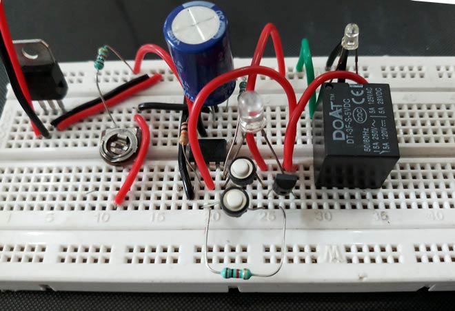
 Simple Time Delay Circuit using 555 TimerIn this project we are going to design a Simple Time Delay Circuit Using 555 Timer IC. This circuit consists of 2 switches one for start the delay time and other for reset. It also has a potentiometer to adjust the time delay, where you can increase of decrease the time delay by just rotating the potentiometer.


The 555 timer is produced as an eight-pin DIL package containing 25 transistors, two diodes and 16 resistors. The 555 can be used as either an astable timer or a monostable timer.
You can calculate the duration of the mark and the space using the following formulae:
Notice how the switch only needs to be pressed once. When the switch makes contact, the timing process begins. The time period depends on the value of resistor R1 and capacitor C1.
The duration of the period is calculated using the formula:
Op-amps are integrated circuits that cram the equivalent of many transistors, resistors and capacitors into a small silicon chip. They are represented in circuit diagrams as follows:

An op-amp has two separate inputs:


This is achieved by restricting the gain using negative feedback. Part of the output signal is returned to the inverting input. This needs a feedback resistor (Rf) and an input resistor (Rin).
The gain of an op-amp with negative feedback is calculated by:
Gain = -50000 / 5000 = -10.
Gain has no units and is just a mathematical value. The '-' sign shows that the output will always be inverted when compared to the input. This means that the op-amp in this example is functioning as an inverting amplifier.
A common comparator is the temperature controller or thermostat on a central heating system. This uses a circuit containing a thermistor to sense temperature and an op-amp. The non-inverting input is set so that the signal going in to it is the same as a particular temperature (say 20°C). The op-amp compares this reference temperature to the actual temperature of the room. If the voltage at the non-inverting input is greater than the voltage at the inverting input, this means that the room is less than the set temperature, and the op-amp switches on the heating system.
The diagram shows an op-amp used as a temperature controller with a thermistor providing the non-inverting input.

The most common counter is the 4017 decade counter IC, which can be set to count to any value between one and 10, over and over again.
A decade counter has 10 outputs. When it is turned on, the counter switches from one output to the next. The speed at which each output turns on or 'goes high' is determined by a timer connected to an input. The counter is switched on and off using either a manual switch or with an astable 555 timer (using pin 3 on the 555 as the output).
Below is a pin-out diagram showing the arrangement of pins in a 4017 counter chip, and a guide to what each pin does.


Integrated circuits (ICs) are self-contained circuits with many separate components such as transistors, diodes, resistors and capacitors etched into a tiny silicon chip.

The chip inside an IC is usually packaged inside a piece of black plastic with tiny pins protruding to allow connections to the circuit. In ICs the pins are arranged in a dual-in-line (DIL) configuration.
The DIL-configuration IC can be used with an IC socket. This prevents damage to the IC caused by heat when manual soldering. It also allows the IC to be changed if necessary, for example during a repair.
ICs can also be configured as a surface-mount chip with either 8, 14 or 16 pins. The surface mount chip is much smaller and is designed for machines to build the circuits.
XXX . XXX 4%zero null 0 SUGGESTED TRIGGER LOGIC AND ELECTRONICS
This is a suggested logic setup for the GEN experiment. The basic trigger is a coincidence between an electron in the HMS (e) and an event in the neutron detector bars (N). If charged particle rates are high, a veto on the paddles (P) may be necessary. In addition, we need to record pedestals (PED)and laser-driven (L) events, and a cosmic ray (C) trigger may be useful to exercise the detector when the beam is off. The logic shown here is designed to minimize transit time of the signal through the logic. It also assumes that no CAMAC reads will be made on an event-by-event basis, so all event information is to be stored in Fast Bus TDCs and ADCs. Main logic Figure 1 shows the main logic. The signals from the neutron bars and paddles are fed to LRS4413 discriminators, set to 25ns width, to allow proper overlap in succeeding circuits. LRS4516 logic circuits form two-fold coincidences between the ends. The 1-8 and 9-16 ORs (on NIM cable) are then sent to an LRS4564. The bars use inputs A1-A10, and the paddles input C1-C5. The OR output of the A section is jumpered to output 13, which is set to 30 ns, while the OR output of the C section is jumpered to output 14. These two signals go to a P7126 ECL-NIM converter, as the 'N' ('nucleon' bar) and 'P' (paddle) signals. The N and P signals then go as NIM signals to the input of the Trigger Supervisor circuits, and to the retiming circuits. Figure 1 -- Main trigger logic
Function of units
Calibration trigger logic Being worked on. Figure 3 shows a suggested cosmic ray trigger, using the paddles and the second neutron bar layer in coincidence. Pedestal triggers may come from the HMS pedestal trigger system, and laser triggers would come from a diode or PMT looking at the laser. Possibly the PMT would be in the neutron cave.
Figure 3 -- Calibration trigger logic

XXX . XXX 4% zero null 0 1 2 3 4 Image stabilization
The explanation triggering and stabilization on Image :
Image stabilization (IS) is a family of techniques that reduce blurring associated with the motion of a camera or other imaging device during exposure. Generally, it compensates for pan and tilt (angular movement, equivalent to yaw and pitch) of the imaging device, though electronic image stabilization can also compensate for rotation. It is used in image-stabilized binoculars, still and video cameras, astronomical telescopes, and also smartphones, mainly the high-end. With still cameras, camera shake is particularly problematic at slow shutter speeds or with long focal length (telephoto or zoom) lenses. With video cameras, camera shake causes visible frame-to-frame jitter in the recorded video. In astronomy, the problem of lens-shake is amplified by variation in the atmosphere over time, which changes the apparent positions of objects over time.
The rule of thumb to determine the slowest shutter speed possible for hand-holding without noticeable blur due to camera shake is to take the reciprocal of the 35 mm equivalent focal length of the lens, also known as the "1/mm rule". For example, at a focal length of 125 mm on a 35 mm camera, vibration or camera shake could affect sharpness if the shutter speed is slower than 1/125 second. As a result of the 2–4.5 stops slower shutter speeds allowed by IS, an image taken at 1/125 second speed with an ordinary lens could be taken at 1/15 or 1/8 second with an IS-equipped lens and produce almost the same quality. The sharpness obtainable at a given speed can increase dramatically. When calculating the effective focal length, it is important to take into account the image format a camera uses. For example, many digital SLR cameras use an image sensor that is 2/3, 5/8, or 1/2 the size of a 35 mm film frame. This means that the 35 mm frame is 1.5, 1.6, or 2 times the size of the digital sensor. The latter values are referred to as the crop factor, field-of-view crop factor, focal-length multiplier, or format factor. On a 2x crop factor camera, for instance, a 50 mm lens produces the same field of view as a 100 mm lens used on a 35 mm film camera, and can typically be handheld at 1/100 of a second.
However, image stabilization does not prevent motion blur caused by the movement of the subject or by extreme movements of the camera. Image stabilization is only designed for and capable of reducing blur that results from normal, minute shaking of a lens due to hand-held shooting. Some lenses and camera bodies include a secondary panning mode or a more aggressive 'active mode', both described in greater detail below under optical image stabilization.
Image-stabilization features can also be a benefit in astrophotography, when the camera is technically—but not effectively—fixed in place. The Pentax K-5 and K-r can use their sensor-shift capability to reduce star trails in reasonable exposure times, when equipped with the O-GPS1 GPS accessory for position data. In effect, the stabilization compensates for the Earth's motion, not the camera's.
There are two types of implementation—lens-based, or body-based stabilization. These refer to where the stabilizing system is located. Both have their advantages and disadvantages.
An optical image stabilizer, often abbreviated OIS, IS, or OS, is a mechanism used in a still camera or video camera that stabilizes the recorded image by varying the optical path to the sensor. This technology is implemented in the lens itself, as distinct from in-body image stabilization, which operates by moving the sensor as the final element in the optical path. The key element of all optical stabilization systems is that they stabilize the image projected on the sensor before the sensor converts the image into digital information.
Different companies have different names for the OIS technology, for example:
Mainly for using video while walking to compensate jitter, Panasonic introduced Power Hybrid O.I.S + with 5-axis correction: axis rotation, horizontal rotation, vertical rotation, horizontal and vertical.
Some of Nikon's more recent VR-enabled lenses offer an "active" mode for shooting from a moving vehicle, such as a car or boat, which is supposed to correct for larger shakes than the "normal" mode. However, active mode used for normal shooting can produce poorer results than normal mode. This is because active mode is optimized for reducing higher angular velocity movements (typically when shooting from a heavily moving platform using faster shutter speeds), where normal mode tries to reduce lower angular velocity movements over a larger amplitude and timeframe (typically body and hand movement when standing on a stationary or slowly moving platform while using slower shutter speeds).
Most manufacturers suggest that the IS feature of a lens be turned off when the lens is mounted on a tripod as it can cause erratic results and is generally unnecessary. Many modern image stabilization lenses (notably Canon's more recent IS lenses) are able to auto-detect that they are tripod-mounted (as a result of extremely low vibration readings) and disable IS automatically to prevent this and any consequent image quality reduction.The system also draws battery power, so deactivating it when not needed extends the battery charge.
A disadvantage of lens-based image stabilization is cost. Each lens requires its own image stabilization system. Also, not every lens is available in an image-stabilized version. This is often the case for fast primes and wide-angle lenses. However, the fastest lens with image stabilization is the Nocticron with a speed of f/1.2. While the most obvious advantage for image stabilization lies with longer focal lengths, even normal and wide-angle lenses benefit from it in low-light applications.
Lens-based stabilization also has advantages over in-body stabilization. In low-light or low-contrast situations, the autofocus system (which has no stabilized sensors) is able to work more accurately when the image coming from the lens is already stabilized. In cameras with optical viewfinders, the image seen by the photographer through the stabilized lens (as opposed to in-body stabilization) reveals more detail because of its stability, and it also makes correct framing easier. This is especially the case with longer telephoto lenses. This advantage does not occur on compact system cameras, because the sensor output to the screen or electronic viewfinder would be stabilized.
The advantage with moving the image sensor, instead of the lens, is that the image can be stabilized even on lenses made without stabilization. This may allow the stabilization to work with many otherwise-unstabilized lenses, and reduces the weight and complexity of the lenses. Further, when sensor-based image stabilization technology improves, it requires replacing only the camera to take advantage of the improvements, which is typically far less expensive than replacing all existing lenses if relying on lens-based image stabilization. Some sensor-based image stabilization implementations are capable of correcting camera roll rotation, a motion that is easily excited by pressing the shutter button. No lens-based system can address this potential source of image blur. A by-product of available "roll" compensation is that the camera can automatically correct for tilted horizons in the optical domain, provided it is equipped with an electronic spirit level, such as the Pentax K-7/K-5 cameras.
One of the primary disadvantages of moving the image sensor itself is that the image projected to the viewfinder is not stabilized. However, this is not an issue on cameras that use an electronic viewfinder (EVF), since the image projected on that viewfinder is taken from the image sensor itself. Similarly, the image projected to a phase-detection autofocus system, if used, is not stabilized.
Some, but not all, camera-bodies capable of in-body stabilization can be pre-set manually to a given focal length. Their stabilization system corrects as if that focal length lens is attached, so the camera can stabilize older lenses, and lenses from other makers. This isn't viable with zoom lenses, because their focal length is variable. Some adapters communicate focal length information from the maker of one lens to the body of another maker. Some lenses that do not report their focal length can have a chip added to the lens, which reports a pre-programmed focal-length to the camera body. Sometimes, none of these techniques works, and image-stabilization simply cannot be used with such lenses.
In-body image stabilization requires the lens to have a larger output image circle because the sensor is moved during exposure and thus uses a larger part of the image. Compared to lens movements in optical image stabilization systems the sensor movements are quite large, so the effectiveness is limited by the maximum range of sensor movement, where a typical modern optically-stabilized lens has greater freedom. Both the speed and range of the required sensor movement increase with the focal length of the lens being used, making sensor-shift technology less suited for very long telephoto lenses, especially when using slower shutter speeds, because the available motion range of the sensor quickly becomes insufficient to cope with the increasing image displacement.
 Starting with the Panasonic Lumix DMC-GX8, announced in July 2015, and subsequently in the Panasonic Lumix DC-GH5, Panasonic, who formerly only equipped lens-based stabilization in its interchangeable lens camera system (of the Micro Four Thirds standard), introduced sensor-shift stabilization that works in concert with the existing lens-based system ("Dual IS").
In the mean time (2016), Olympus is also offering two lenses with image stabilization that can be synchronized with the in-built image stabilization system of the image sensors of Olympus' Micro Four Thirds cameras ("Sync IS"). With this technology a gain of 6.5 f-stops can be achieved without blurred images. This is limited by the rotational movement of the surface of the Earth, that fools the accelerometers of the camera. Therefore, depending on the angle of view, the maximum exposure time should not exceed 1/3 second for long telephoto shots (with a 35-mm equivalent focal length of 800 millimeters) and a little more than ten seconds for wide angle shots (with a 35-mm equivalent focal length of 24 millimeters), if the movement of the Earth is not taken into consideration by the image stabilization process.
In 2015, the Sony E camera system also allowed the combination of the image stabilization systems of lenses and camera bodies, but without synchronizing the same degrees of freedom. In this case only the independent compensation degrees of the in-built image sensor stabilization will be activated to support lens stabilization.
Some still camera manufacturers marketed their cameras as having "digital image stabilization" when they really only had a high-sensitivity mode that uses a short exposure time—producing pictures with less motion blur, but more noise. It reduces blur when photographing something that is moving, as well as from camera shake.
Others now also use digital signal processing (DSP) to reduce blur in stills, for example by sub-dividing the exposure into several shorter exposures in rapid succession, discarding blurred ones, re-aligning the sharpest sub-exposures and adding them together, and using the gyroscope to detect the best time to take each frame.
Online services, including Google's YouTube, are also beginning to provide video stabilization as a post-processing step after content is uploaded. This has the disadvantage of not having access to the realtime gyroscopic data, but the advantage of more computing power and the ability to analyze images both before and after a particular frame.
This has been integrated into camcorders by allowing the sensor and lens assembly to move together within the camera housing.
Another technique for stabilizing a video or motion picture camera body is the Steadicam system, which isolates the camera from the operator's body using a harness and a camera boom with a counterweight.
In close-up photography, using rotation sensors to compensate for changes in camera-pointing-direction becomes insufficient. Moving, rather than tilting, the camera up/down or left/right by a fraction of a millimeter becomes noticeable if you are trying to resolve millimeter-size details on the object. Linear accelerometers in the camera, coupled with information such as the lens focal length and focused distance, can feed a secondary correction into the drive that moves the sensor or optics, to compensate for linear as well as rotational shake.
++++++++++++++++++++++++++++++++++++++++++++++++++++++++++++++++++++++
TRIGGERING AND STABILIZATION ON ELECTRONICs MEDIUM CIRCUIT

+++++++++++++++++++++++++++++++++++++++++++++++++++++++++++++++++++++++

| Trigger condition | Description |
|---|---|
| None | there is no additional trigger condition. |
| Shorter than | the signal requirements defined by the trigger type must last shorter than the specified trigger condition time to cause a trigger. |
| Longer than | the signal requirements defined by the trigger type must last longer than the specified trigger condition time to cause a trigger. |
| Inside | the length that the signal requirements defined by the trigger type last, must be inside the trigger condition time frame to cause a trigger. |
| Outside | the length that the signal requirements defined by the trigger type last, must be shorter than or longer than the trigger condition time frame, in other words outside the trigger condition time frame to cause a trigger. |
- Using the Condition selector in the trigger properties dialog.
- Right-clicking the trigger symbol on an axis or the associated channel in the Object Tree and selecting Trigger condition and then the required value in the popup menu.
Trigger condition time(s)
The trigger condition time specifies the duration of a specific signal condition, in seconds. When two trigger condition times are available, the two times define a trigger condition time frame, in seconds.
Setting the trigger condition time(s) in the Multi Channel oscilloscope software can be done in several ways:
- Entering the required value in the Condition time or Condition time 2 box in the trigger properties dialog.
- Right-clicking the trigger symbol on an axis or the associated channel in the Object Tree and selecting Trigger condition time or Trigger condition time 2 in the popup menu. The time is entered in seconds.
XXX . XXX Digital data acquisition
All digital oscilloscopes measure by sampling the analog input signals and digitizing the values.
Sampling
When an oscilloscope samples an input signal, samples are taken at fixed intervals. At these intervals, the size of the input signal is converted to a number. The accuracy of this number depends on the resolution of the oscilloscope. The higher the resolution, the smaller the voltage steps in which the input range of the instrument is divided. The acquired numbers can be used for various purposes, e.g. to create a graph.
 The sine wave in the above picture is sampled at the dot positions. By connecting the adjacent samples, the original signal can be reconstructed from the samples. You can see the result in the next illustration.

Sample frequency
The rate at which samples are taken by the oscilloscope is called the sample frequency, the number of samples per second. A higher sample frequency corresponds to a shorter interval between the samples. As is visible in the picture below, with a higher sample frequency, the original signal can be reconstructed much better from the measured samples.
 The sample frequency must be higher than 2 times the highest frequency in the input signal. This is called the Nyquist frequency. Theoretically it is possible to reconstruct the input signal with more than 2 samples per period. In practice, at least 10 to 20 samples per period are recommended to be able to examine the signal thoroughly in an oscilloscope. When the sample frequency is not high enough, aliasing will occur.
Changing the sample frequency of an instrument in the Multi Channel oscilloscope software can be done in various different ways:
Changing the sample frequency of an instrument in the Multi Channel oscilloscope software can be done in various different ways:
- Clicking the Sample frequency indicator
 on the channel toolbar and selecting the required sample frequency from the popup menu
 - Clicking the decrease/increase sample frequency buttons
 and
and  on the instrument toolbar
 - Using hotkeys F3 (lower) and F4 (higher).
- Clicking the Sample frequency label in the combined Record length + Sample frequency + Resolution indicator
 on the instrument toolbar and selecting the required value from the popup menu.
 - Right-clicking the horizontal scrollbar under the graph displaying signals from the instrument and selecting Sample frequency and then the appropriate value in the popup menu.
- Right-clicking the instrument in the Object Tree, selecting Sample frequency and then the appropriate sample frequency value in the popup menu
Depending on the instrument settings, the instrument can have certain limitations with respect to the available sample frequencies. When a user defined value is requested that is not available, the software will use the closest available value.
Aliasing
When sampling an analog signal with a certain sampling frequency, signals appear in the output with frequencies equal to the sum and difference of the signal frequency and multiples of the sampling frequency. For example, when the sampling frequency is 1000 Hz and the signal frequency is 1250 Hz, the following signal frequencies will be present in the output data:
As stated before, when sampling a signal, only frequencies lower than half the sampling frequency can be reconstructed. In this case the sampling frequency is 1000 Hz, so we can we only observe signals with a frequency ranging from 0 to 500 Hz. This means that from the resulting frequencies in the table, we can only see the 250 Hz signal in the sampled data. This signal is called an alias of the original signal.
If the sampling frequency is lower than 2 times the frequency of the input signal, aliasing will occur. The following illustration shows what happens.
 In this picture, the green input signal (top) is a triangular signal with a frequency of 1.25 kHz. The signal is sampled with a frequency of 1 kHz. The corresponding sampling interval is 1/( 1000 Hz ) = 1 ms. The positions at which the signal is sampled are depicted with the blue dots.
The red dotted signal (bottom) is the result of the reconstruction. The period time of this triangular signal appears to be 4 ms, which corresponds to an apparent frequency (alias) of 250 Hz (1.25 kHz - 1 kHz).
In practice, to avoid aliasing, always start measuring at the highest sampling frequency and lower the sampling frequency if required. Use function keys F3 (lower) and F4 (higher) to change the sampling frequency in a quick and easy way. The next illustration gives an example of what aliasing can look like.
 In this picture, a sine wave signal with a frequency of 257 kHz is sampled at a frequency of 50 kHz. The minimum sampling frequency for correct reconstruction is 514 kHz. For proper analysis, the sampling frequency should have been approximately 5 MHz.
| Multiple of sampling frequency | 1250 Hz signal | -1250 Hz signal | ||
|---|---|---|---|---|
| ... | ||||
| -1000 | -1000 + 1250 = | 250 | -1000 - 1250 = | -2250 |
| 0 | 0 + 1250 = | 1250 | 0 - 1250 = | -1250 |
| 1000 | 1000 + 1250 = | 2250 | 1000 - 1250 = | -250 |
| 2000 | 2000 + 1250 = | 3250 | 2000 - 1250 = | 750 |
| ... | ||||
If the sampling frequency is lower than 2 times the frequency of the input signal, aliasing will occur. The following illustration shows what happens.
The red dotted signal (bottom) is the result of the reconstruction. The period time of this triangular signal appears to be 4 ms, which corresponds to an apparent frequency (alias) of 250 Hz (1.25 kHz - 1 kHz).
In practice, to avoid aliasing, always start measuring at the highest sampling frequency and lower the sampling frequency if required. Use function keys F3 (lower) and F4 (higher) to change the sampling frequency in a quick and easy way. The next illustration gives an example of what aliasing can look like.
Record Length
With a given sampling frequency, the number of samples that is taken determines the duration of the measurement. This number of samples is called record length. Increasing the record length, will increase the total measuring time. The result is that more of the measured signal is visible. In the images below, three measurements are displayed, one with a record length of 12 samples, one with 24 samples and one with 36 samples.


 The total duration of a measurement can easily be calculated, using the sampling frequency and the record length:
Measurement duration in seconds = record length in samples / sampling frequency in Hz
Changing the record length of an instrument in the Multi Channel oscilloscope software can be done in various different ways: - Clicking the Record length indicator
 on the instrument toolbar and selecting the required value from the popup menu.
 - Clicking the decrease/increase record length buttons
 and
and  on the instrument toolbar.
 - Using hotkeys F11 (shorter) and F12 (longer).
- Clicking the Record length label in the combined Record length + Sample frequency + Resolution indicator on the instrument toolbar and selecting the required value from the popup menu.
- Right-clicking the horizontal scrollbar under the graph displaying signals from the instrument and selecting Record length and then the appropriate value in the popup menu.
- Right-clicking the instrument in the Object Tree, selecting Record length and then the appropriate value in the popup menu.
Depending on the instrument settings, the instrument can have certain limitations with respect to the available record lengths. When a user defined value is requested that is not available, the software will use the closest available value.
Time base
The combination of sampling frequency and record length forms the time base of an oscilloscope. To setup the time base properly, the total measurement duration and the required time resolution have to be taken in account.
There are several ways to find the required time base setting. With the required measurement duration and sampling frequency, the required number of samples can be determined:
The Multi Channel oscilloscope software also provides controls to change record length and sample frequency simultaneously to specific combinations to obtain certain time/div values:
There are several ways to find the required time base setting. With the required measurement duration and sampling frequency, the required number of samples can be determined:
record length in samples = Measurement duration in seconds * sampling frequency in Hz
With a known record length in samples and the required measurement duration, the necessary sampling frequency can be calculated: sampling frequency in Hz = record length in samples / Measurement duration in seconds
In the Multi Channel oscilloscope software, both record length and sampling frequency can be set independently, to give the best flexibility. They can be selected from menu's, using toolbar buttons but also keyboard short cuts are available, for more information, refer to: The Multi Channel oscilloscope software also provides controls to change record length and sample frequency simultaneously to specific combinations to obtain certain time/div values:
- Clicking the decrease/increase Time/div buttons
 and
and  on the instrument toolbar.
 - Clicking the Time/div indicator
 on the instrument toolbar and selecting the required time/div value from the popup menu.
 - Using hotkeys Ctrl + F11 (lower) and Ctrl + F12 (higher)
Resolution
When digitizing the samples, the voltage at each sample time is converted to a number. This is done by comparing the voltage with a number of levels. The resulting number is the number of the highest level that's still lower than the voltage. The number of levels is determined by the resolution. The higher the resolution, the more levels are available and the more accurate the input signal can be reconstructed. In the image below, the same signal is digitized, using three different amounts of levels: 16, 32 and 64.


 The number of available levels is determined by the resolution:
The used resolutions in the previous image are respectively: 4 bits, 5 bits and 6 bits.
The smallest detectable voltage difference depends on the resolution and the input range. This voltage can be calculated as:
Changing the resolution of an instrument in the Multi Channel oscilloscope software can be done in various different ways:
number of levels = 2 resolution in bits The used resolutions in the previous image are respectively: 4 bits, 5 bits and 6 bits.
The smallest detectable voltage difference depends on the resolution and the input range. This voltage can be calculated as:
minimum voltage = full scale range / number of levels
In the 200 mV range, the full scale ranges from -200 mV to +200 mV, the full range is 400 mV. When a 12 bit resolution is used, there are 212 = 4096 levels. This results in a smallest detectable voltage step of 0.400 V / 4096 = 97.7 µV. In 16 bit resolution this step is 0.400 V / 65536 = 6.1 µV Changing the resolution of an instrument in the Multi Channel oscilloscope software can be done in various different ways:
- Right-clicking the instrument in the Object Tree, selecting Resolution and then the appropriate resolution value in the popup menu
- Clicking the decrease/increase resolution buttons
 and
and  on the instrument toolbar
 - Clicking the resolution indicator
 on the instrument toolbar and selecting the required resolution from the popup menu
Differential measurements
Voltage is defined as the electrical potential difference between two points. So, when measuring a voltage, it is measured between two points.
Single ended oscilloscope inputs
Most oscilloscopes are equipped with standard, single ended inputs, which are referenced to ground. This means that one side of the input is always connected to ground and the other side to the point of interest in the circuit under test.
 Therefore the voltage that is measured with an oscilloscope with standard, single ended inputs is always measured between that specific point and ground.
What if the voltage you're interested in is not referenced to ground? Connecting a standard single ended oscilloscope input to the two points would create a short circuit between one of the points and ground, possibly damaging the circuit and the oscilloscope.
A safe way would be to measure the voltage at one of the two points, in reference to ground and at the other point, in reference to ground and then calculate the voltage difference between the two points. On most oscilloscopes this can be done by connecting one of the channels to one point and another channel to the other point and then use the math function Ch1 - Ch2 in the oscilloscope to display the actual voltage difference.
 There are some disadvantages to this method:
What if the voltage you're interested in is not referenced to ground? Connecting a standard single ended oscilloscope input to the two points would create a short circuit between one of the points and ground, possibly damaging the circuit and the oscilloscope.
A safe way would be to measure the voltage at one of the two points, in reference to ground and at the other point, in reference to ground and then calculate the voltage difference between the two points. On most oscilloscopes this can be done by connecting one of the channels to one point and another channel to the other point and then use the math function Ch1 - Ch2 in the oscilloscope to display the actual voltage difference.
- to measure one signal, two channels are occupied.
- by using two channels, the measurement error is increased, the errors made on each channel will be combined, resulting in a larger total measurement error.
- The Common Mode Rejection Ratio of this method is relatively low. If both points have a relative high voltage, but the voltage difference between the two points is small, the voltage difference can only be measured in a high input range, resulting in a low resolution.
Differential oscilloscope inputs
Some oscilloscopes are equipped with a differential input. A differential input is not referenced to ground, but both sides of the input are "floating". - No possibility to create a short circuit to ground through the oscilloscope.
- Only one channel is used to measure the signal.
- More accurate measurement, since only one channel introduces a measurement error.
- The Common Mode Rejection Ratio of a differential input is high. If both points have a relative high voltage, but the voltage difference between the two points is small, the voltage difference can be measured in a low input range, resulting in a high resolution.
Applications
There are various applications for oscilloscopes with differential inputs.
Power systems
One applications for oscilloscopes with differential inputs is measurements in (switch mode) power supplies, motor drives, frequency inverters. The high common mode voltages and low voltage differences make an oscilloscope with differential inputs the ideal measuring instrument. It also reduces the risk of creating short circuits, resulting in damaged circuits and/or measuring instruments.
Communication buses
Oscilloscopes with differential inputs can also be used very well when measuring at (high speed) digital communication buses like e.g. USB and CAN.
To improve signal integrity, such buses use two differential signal lines and a common ground line. The two signal lines transport the same signal, with the difference that they are each others inverse. This reduces the effect of external influences, since most external disturbances are additive and cause the same offset error in both signal lines. The voltage difference will remain the same, so the actual signal is not affected. To measure the actual signal, a differential input is required.
To improve signal integrity, such buses use two differential signal lines and a common ground line. The two signal lines transport the same signal, with the difference that they are each others inverse. This reduces the effect of external influences, since most external disturbances are additive and cause the same offset error in both signal lines. The voltage difference will remain the same, so the actual signal is not affected. To measure the actual signal, a differential input is required.
Audio systems
Another application for oscilloscopes with differential inputs is measuring in professional audio systems. Just as for the digital buses described above, also in professional audio systems two signal lines and a ground line are used to improve the signal integrity (here called "balanced").
Products
TiePie engineering has a number of products for measuring with differential inputs.
SCR Protection Circuits Handyprobe HP3
The Handyprobe HP3 high voltage oscilloscope is a portable USB oscilloscope with a full differential high voltage input that will measure voltages up to 800 V DC / 566 V RMS (CAT II).
 The Handyprobe HP3 high voltage oscilloscope combines a high voltage input with 10 bit resolution, 100 MSamples/second and 1 MSamples record length.
For more information and specifications, refer to the page about the Handyprobe HP3
For more information and specifications, refer to the page about the Handyprobe HP3
Handyscope HS4 DIFF
The Handyscope HS4 DIFF is a powerful computer controlled measuring instrument that features four built-in differential input channels.
 The USB connected Handyscope HS4 DIFF features a user selectable 12 bit, 14 bit or 16 bit resolution, 200 mV to 80 V full scale input range, 128 Ksamples record length per channel and a sampling frequency up to 50 MHz on all four channels simultaneously.
For more information and specifications, refer to the page about the Handyscope HS4 DIFF
For more information and specifications, refer to the page about the Handyscope HS4 DIFF
Differential attenuators
To increase the input range of a differential input, a special differential attenuator is required. For a differential input, both sides of the input need to be attenuated.
 Standard oscilloscope probes and attenuators only attenuate one side of the signal path. These are not suitable to be used with a differential input. Using these on a differential input will have a negative effect on the CMRR and will introduce measurement errors.
 To increase the input range of the Handyscope HS4 DIFF, it comes with four differential 1:10 attenuators, the Differential attenuator TP-DA10. These differential attenuators are specially designed to be used with the Handyscope HS4 DIFF.

Differential measurement cables
The Handyscope HS4 DIFF comes with four special measurement cables, the Measure lead TP-C812B, suitable to perform differential measurements.
 The supplied cables, with a BNC at one end and two banana jacks at the other end, ensure a good CMRR.
Differential probe SI-9002
To provide an existing oscilloscope with one or more differential inputs, the Differential probe SI-9002 is the ideal solution.
 This Differential Probe provides any general oscilloscope with a high voltage differential input. Both the positive and negative sides of the balanced input possess high voltage differential input up to 700 V, and its sensitivity can extend down to 100 mV.

Single-phase electric furnace temperature control with SCR zero trigger circuit using NE555, C302

SCR Control circuits
Single-phase electric furnace temperature control with SCR zero trigger circuit using NE555, C302
9 second digital readout countdown timer
This circuit provides a visual 9 second delay using a 7 segment digital readout LED. When the switch is closed, the CD4010 up/down counter is preset to 9 and the 555 timer is disabled with the output held high.. SCR Control circuits
90° Phase Control of SCR.
 Phase control of SCR

Phase control of SCR
In ac circuits, the SCR can be turned on by the gate at any angle a with respect to the applied voltage. This angle α is called the firing angle. Power control is obtained by varying the firing angle and this is known as phase control. In the phase-control circuit given in fig. 1, the gate triggering voltage is derived from the ac supply through resistors R1, R2 and R3. The variable resistance R2 limits the gate current during positive half cycles of the supply. If the moving contact is set to the top of resistor R2, resistance in the circuit is the lowest and the SCR may trigger almost immediately at the commencement of the positive half cycle of the input. If, on the other hand, the moving contact is set to the bottom of resistor R2, resistance in the circuit is maximum, the SCR may not switch on until the peak of the positive half-cycle. By adjusting R2 between these two extremes, SCR can be switched on somewhere between the commencement and peak of the positive half-cycle, that is between 0° and 90°. If the triggering voltage VT is not large enough to trigger SCR at 90°, the device will not trigger on at all, because VT has the maximum value at the peak of the input and decreases with the fall in voltage. This operation is sometimes referred to as half-wave variable-resistance phase control. It is an effective method of controlling the load power.
Diode D is provided to protect the SCR gate from the negative voltage that would otherwise be applied during the negative half cycle of the input. It can be seen from the circuit diagram shown in fig.a, that at the instant of turning on of the SCR gate current flows through RL and diode. So
VT=VD + VG + IGRL
180 degree Phase Control.
 Phase Control-SCR

Phase Control-SCR
The circuit shown in figure, can trigger the SCR from 0° to 180° of the input waveform. In the circuit shown here, the resistor R and capacitor C determine the point in the input cycle at which the SCR triggers. During the negative half cycle of the input, capacitor C is charged negatively (with the polarity shown in the figure) through diode D2 to the peak of the input voltage because diode D2 is forward-biased. When the peak of the input negative half cycle is passed, diode D2 gets reverse-biased and capacitor C commences to discharge through resistor R. Depending upon the time constant, that is CR, the capacitor C may be almost completely discharged at the commencement of the positive half cycle of the input, or it may retain a partially negative charge until almost 180° of positive half cycle has passed. So long as the capacitor C remains negatively charged, diode D1, is reverse-biased and the gate cannot go positive to trigger the SCR into conduction. Thus R and /or C can be adjusted to affect SCR triggering anywhere from 0° to 180° of the input ac cycle.
Pulse Control of an SCR.
 Pulse Control Circuit

Pulse Control Circuit
The simplest of SCR control circuits is shown in figure. If SCR were an ordinary rectifier, it would develop half-wave rectified ac voltage across the load RL. The same would be true if the gate of the SCR had a continuous bias voltage to keep it on when the anode-cathode voltage VAK goes positive. A trigger pulse applied to the gate can switch the device at any time during the positive half-cycle of the input. The resultant load waveform is a portion of positive half cycle commencing at the instant at which the SCR is triggered. Resistor RG holds the gate-cathode voltage, VG at zero when no trigger input is present. The instantaneous level of load current can/be determined from the following relation
How to protect an SCR using protection circuits ?
SCRs are sensitive to high voltage, over-current, and any form of transients. For satisfactory and reliable operation they are required to be protected against such abnormal operating conditions. Because of complex and expensive protection, usually some margin is provided in the equipment by selecting devices with ratings higher (3 or 4 times higher) than those required for normal operation. But it is always not economical to use devices of higher ratings, hence their protection is imperative.
Over-voltage Protection.
 SCR Over Voltage Protection

SCR Over Voltage Protection
High forward voltage protection is inherent in SCRs. The SCR will breakdown and start conducting before the peak forward voltage is attained so that the high voltage is transferred to another part of the circuit (usually the load). The turn-on of SCR causes a large current to flow and poses a problem of over-current protection.
Over-current Protection.
 SCR Over Current Protection

SCR Over Current Protection
Over-current protection can be provided by connecting a circuit breaker and a fuse in series with the SCR, as usually done for the protection of any circuit. However, there are some reservations to their use. A semiconductor device is capable of taking overloads for a limited period, so the fuse used should have high breaking capacity and rapid interruption of current. There must be a similarity of SCR and fuse I2t rating without developing high voltage transients which endanger those SCRs in the off or infinite impedance condition. These are contradictory requirements necessitating voltage protection when fast-acting fuses are employed. Fuses when used, their arc voltages are kept below 1.5 times the peak circuit voltage. For small power applications it is pointless to employ high speed fuses for circuit protection because it may cost more than the SCR. Current magnitude detection can be employed and is used in many applications. When an over-current is detected the gate circuits are controlled either to turn-off the appropriate SCRs, or in phase commutation, to reduce the conduction period and so the average value of the current.
If the output to the load from the SCR circuit is alternating current, LC resonance provides over-current protection as well as filtering. A current limiting device employing a saturable reactor is shown in figure. With normal currents the saturable reactor L1 offers high impedance and C and L are in series resonance to offer zero impedance to the flow of current of the fundamental harmonic. An over-current saturates L1 and so gives negligible impedance. There is LC parallel resonance and hence infinite impedance to the flow of current at the resonant frequency.
Protection against Voltage Surges.
There are many types of failure due to voltage surges as SCRs do not really have a safety factor included in their ratings. External voltage surges cannot be controlled by the SCR circuit designer. Voltage surges often lead to either malfunctioning of the circuit by unintentional turn-on of SCR or permanent damage to the device due to reverse breakdown. SCR can be protected against voltage surges by employing shunt connected non-linear resistance devices. Such protective devices register a fall in resistance with the increase in voltage and so develop a virtual short-circuit across the SCR when a high voltage is applied. An over-voltage protection circuit employing thyrector-diode, which has low resistance at high voltage and vice-versa, is shown in figure. Inductor L and capacitor C provides protection to SCR against large dV/dt and dI/dt.
XXX . XXX 1 Minute Timer Circuit
1 Minute Timer Circuit using IC 555 As the name suggest 555 timer is basically a “Timer”, which create an oscillating pulse. It means for some time output pin 3 is HIGH and for some time it remains LOW, that will create a oscillating output. We can use this property of 555 timer to create various timer circuits like 1 minute timer circuit, 5 minute timer circuit, 10 minute timer circuit, 15 minute timer circuit, etc. All we need to change the value of Resistor R1 and/or Capacitor C1. We need to set 555 timer in Monostable mode to build Timer. In monostable mode, the duration for which the PIN 3 would remain HIGH, is given by the below formulae:
T = 1.1 * R1*C1
So to build 1 minute (60 seconds) timer we need resistor of value 55k ohm and capacitor of 1000uF:
1.1*55k*1000uF
(1.1*55*1000*1000)/1000000 = 60.5 ~ 60 seconds.

A variable resistor of 1M is used here and set on 55k ohm (measured by multimeter). We can easily calculate the resistor value for 5 minute, 10 minute and 15 minute timer circuit:
5*60 = 1.1 * R1 * 1000 uF
R1 = 272.7 k ohm
So to build a 5 minute timer circuit, we would be simply changing the resitor value to 272.7k ohm in above given 1 minute timer circuit.
10 Minute Timer Circuit
10*60 = 1.1*R1*1000 uF
R1 = 545.4 k ohm
Similarly to create a 10 minute timer we would be changing the resistor value to 545.4 k ohm.
15 Minute Timer Circuit
15*60 = 1.1*R1*1000 uF
R1 = 818.2 k ohm
As per above calculations, for a 15 minute timer circuit, we need the value of resistor to 818.2k ohm.
We should note here that we have used LED at reverse logic, means when OUTPUT pin 3 is low, LED will be ON, and when OUTPUT is HIGH then LED will be OFF. So we have calculated OFF time above, means after the calculated time LED will be turned ON. LED will be ON initially (OUTPUT PIN 3 LOW), as soon as we press push button (trigger the 555 via TRIGGER PIN 2), the timer will start, and LED will become OFF (OUTPUT PIN 3 LOW), after the calculated time duration, PIN 3 will again become LOW, and LED get turned ON.
Here we have used 9 V battery and 5V optional relay for switching the AC load. A 5v voltage regulator is used for giving 5v regular supply to the circuit. Also check our 1 minute timer circuit using 555.
Required Components:
- 555 timer IC
- Resistor- 1k (3)
- Resistor- 10k
- Variable Resistor – 1000k
- Capacitor – 200uF, 0.01uF
- LED- Red and green
- Push Buttons- 2
555 Timer IC:
Before going into detail of Time Delay Circuit, first we need to learn about 555 Timer IC first.
Pin 1. Ground: This pin should be connected to ground.
Pin 2. TRIGGER: Trigger pin is dragged from the negative input of comparator two. The comparator two output is connected to SET pin of flip-flop. With the comparator two output high we get high voltage at the timer output. If this pin is connected to ground (or less than Vcc/3), the output will be always high.
Pin 3. OUTPUT: This pin also has no special function. This is output pin where Load is connected.
Pin 4. Reset: There is a flip-flop in the timer chip. Reset pin is directly connected to MR (Master Reset) of the flip-flop. This pin is connected to VCC for the flip-flop to stop from hard resetting.
Pin 5. Control Pin: The control pin is connected from the negative input pin of comparator one. Normally this pin is pulled down with a capacitor (0.01uF), to avoid unwanted noise interference with the working.
Pin 6. THRESHOLD: Threshold pin voltage determines when to reset the flip-flop in the timer. The threshold pin is drawn from positive input of comparator1. If the control pin is open. Then a voltage equal to or greater than VCC*(2/3) (i.e.6V for a 9V supply) will reset the flip-flop. So the output goes low.
Pin 7. DISCHARGE: This pin is drawn from the open collector of transistor. Since the transistor (on which discharge pin got taken, Q1) got its base connected to Qbar. Whenever the output goes low or the flip-flop gets reset, the discharge pin is pulled to ground.
Pin 8. Power or VCC: It is connected to positive voltage (+3.6v to +15v).
Monostable Mode of 555 Timer IC:
555 Timer IC is configured in the Monostable mode for this Time Delay circuit. So here we are explaining the Monostable mode of 555 Timer IC.
Below is the Internal structure of 555 Timer IC:
Operation is simple, initially 555 is in stable state i.e. OUPUT at PIN 3 is low. We know that Non-inverting end of Lower Comparator is at 1/3Vcc, so when we apply negative (< 1/3Vcc) voltage to the Trigger PIN 2 by connecting it to Ground (through a PUSH button switch), two things happens:
- First is, Lower comparator becomes HIGH and Flip flop gets Set and we get HIGH OUTPUT at PIN 3.
- And second thing is, Transistor Q1 becomes OFF, and Timing capacitor C1 get disconnected from the Ground and start charging though the Resistor R1.
This state is called the quasi stable state and remains for some time (T). Now when capacitor starts charging and reaches to the voltage slightly greater than 2/3 Vcc, voltage at Threshold PIN 6 becomes greater than the voltage at inverting end (2/3Vcc) of Upper comparator, again two things happens:
- Firstly, Upper comparator becomes HIGH and Flip flop gets Resets and the OUTPUT of the chip at PIN 3 becomes LOW.
- And secondly, Transistor Q2 becomes ON, and capacitor starts discharging to the ground, through the Discharge PIN 7.
So 555 IC automatically fall back to the stable state (LOW) after the time determined by the RC network. This duration of quasi stable state can be calculated using this 555 Monostable Calculator or can be calculated with the formulae given below:
T= 1.1*R1*C1 Seconds where R1 is in OHM and C1 is in Farads.
So now we can see that MONOSTABLE mode has only one stable state and require a negative pulse at PIN 2, for the transition to Quasi stable state. Quasi stable state only remains for 1.1*R1*C1 seconds and then it automatically switch back to stable state. Remember one thing, while designing this circuit, that Trigger pulse at PIN 2 must be shorter enough to the OUPUT pulse, so that the capacitor gets enough time to charge and discharge.
Circuit Diagram:
Below is the Circuit Diagram for Simple Delay Circuit using 555 IC:

Working of Time Delay Circuit:
The entire circuit is powered by 5V using 7805 voltage regulator. Initially when no button is pressed the output of the 555 IC remains LOW and the circuit remains in this state, until you press the START button and the capacitor C1 remains in discharged condition.
As we explained above, the time delay for the quasi stable state (unstable) is depend upon the value Timing capacitor and resistor. As you change the value of these, the time delay for quasi stable state will also be changed. Here the Blue LED glows in quasi stable state for the particular time and Red LED glows in stable state. So here we have replaced this timing Resistor with the Variable Resistor, so that we can adjust the time delay just by rotating the knob of potentiometer on the board itself. Here we have also connected a optional Relay for triggering the AC appliance after a the time delay.
When you press the Start button, the countdown timer starts and Blue LED turns on and after the particular time (defined by the formula T= 1.1*R1*C1) the 555 timer goes in stable state, where Red LED turns ON and blue LED turns Off. You can increase and decrease the time delay by using the potentiometer .
Timer circuits
Timer circuits are used to control sequences of events in electronic systems by changing the circuit from one state to another at preset times.The 555 timer is produced as an eight-pin DIL package containing 25 transistors, two diodes and 16 resistors. The 555 can be used as either an astable timer or a monostable timer.
An astable timer
An astable circuit is a useful process block that is often called a pulse generator. When the astable timer is switched on it will give a constant on/off digital output. So the timer will make a LED flash, at a rate determined by a capacitor in the circuit.Mark/space time
The period when the timer/LED is on is called the mark and the period when the timer/LED is off is called the space. The mark and the space can be set to be the same or they can be different. If they are the same, then the on and off times of the pulse will be equal. If they are different, then the on and off will not be equal: eg there might be a short pulse, followed by a long space before the next one.You can calculate the duration of the mark and the space using the following formulae:
Mark (time on) = 0.7 x (R1 + R2) x C1
Space (time off) = 0.7 x R1 x C1
R1 is the value of resistor R1 (in ohms), R2 is value of resistor R2 (in ohms) and C1 is the value of the capacitor (in microfarads). The frequency can be adjusted by changing the values of R1, R2 and C1. The ratio of the mark to space (time on to time off) can be changed by changing the value of R2.Space (time off) = 0.7 x R1 x C1
A monostable timer
Monostable timers are often called one-shot timers. When the timer is switched on it will stay on for a certain length of time and then stay off until it is switched on again.Notice how the switch only needs to be pressed once. When the switch makes contact, the timing process begins. The time period depends on the value of resistor R1 and capacitor C1.
The duration of the period is calculated using the formula:
Time on (seconds) = 1.1 x R1 x C1
R1 is the value of resistor R1 (in ohms) and C1 is the value of the capacitor (in microfarads).Two examples
- Question
- An astable 555 timer has the following external component values: R1 = 100 kilo-ohms; R2 = 47 kilo-ohms; C1 = 10 microfarads. What is the mark and space?
- Answer
- Mark (time on) = 0.7 x (100,000 + 47,000) x 0.00001 = 1 second
Space (time off) = 0.7 x 100,000 x 0.00001 = 0.7 seconds
- Question
- A monostable 555 timer has the following component values: R1 is 100 kilo-ohms and C1 is 100 microfarads. Calculate the length of time that the timer will stay on.
- Answer
- Time on = 1.1 x 100 000 x 0.0001 = 11 seconds .
Operational amplifiers
Amplifiers are devices which take a relatively weak signal as an input and produce a much stronger signal as an output. The operational amplifier (or op-amp) is a special kind of amplifier used in equipment such as stereo equipment and medical cardiographs (which amplify the heart beat).Op-amps are integrated circuits that cram the equivalent of many transistors, resistors and capacitors into a small silicon chip. They are represented in circuit diagrams as follows:
An op-amp has two separate inputs:
- the inverting input
- the non-inverting input
Operational amplifier circuit diagram
- Offset/null
- Inverting input
- Non-inverting input
- Negative supply
- Not used
- Output
- Positive supply
- Offset/null
Gain of an op-amp
Op-amps have a voltage gain of 100,000. This makes them very sensitive to small changes. For example, a difference between the input pins of just 0.0001 V would give a potential change in output of more that the full power supplied to the circuit by a 9V battery. Sometimes it is necessary to make them less sensitive, so that larger changes can be reliably detected.Using negative feedback to control the gain of an op-amp
This is achieved by restricting the gain using negative feedback. Part of the output signal is returned to the inverting input. This needs a feedback resistor (Rf) and an input resistor (Rin).
The gain of an op-amp with negative feedback is calculated by:
Gain = -Rf / Rin
For example, where Rf = 50 kilo-ohms and Rin = 5 kilo-ohms:Gain = -50000 / 5000 = -10.
Gain has no units and is just a mathematical value. The '-' sign shows that the output will always be inverted when compared to the input. This means that the op-amp in this example is functioning as an inverting amplifier.
Op-amps as comparators
Op-amps are often used as comparators. This means that they are used to compare two inputs (the inverting input and the non-inverting input).A common comparator is the temperature controller or thermostat on a central heating system. This uses a circuit containing a thermistor to sense temperature and an op-amp. The non-inverting input is set so that the signal going in to it is the same as a particular temperature (say 20°C). The op-amp compares this reference temperature to the actual temperature of the room. If the voltage at the non-inverting input is greater than the voltage at the inverting input, this means that the room is less than the set temperature, and the op-amp switches on the heating system.
The diagram shows an op-amp used as a temperature controller with a thermistor providing the non-inverting input.
Counter circuits
Counter circuits record the number of times an event takes place.The most common counter is the 4017 decade counter IC, which can be set to count to any value between one and 10, over and over again.
A decade counter has 10 outputs. When it is turned on, the counter switches from one output to the next. The speed at which each output turns on or 'goes high' is determined by a timer connected to an input. The counter is switched on and off using either a manual switch or with an astable 555 timer (using pin 3 on the 555 as the output).
Below is a pin-out diagram showing the arrangement of pins in a 4017 counter chip, and a guide to what each pin does.
- Pins 1 to 7 and pin 9 and pin 11 are outputs for the counter.
- Pin 8 is the negative power supply.
- Pin 12 is the carry-out pin (this could be connected to another 4017).
- Pin 13 is the enable pin. It can be used to stop the count.
- Pin 14 is the clock pin. This will be connected to a manual switch or to an astable 555 timer.
- Pin 15 is the reset pin. This returns counter to zero. The counter can be made to count to numbers less than 10 by the count number above the maximum required to pin 15.
- Pin 16 is the positive power supply pin. It runs at a voltage between 3V and 16V.
Integrated circuits are the basic component of modern microelectronics. They are important process blocks in electronic systems. There is a wide range of integrated circuits available, including timer circuits, operational amplifiers and counter circuits.
Advantages of integrated circuits
Integrated circuits (ICs) are self-contained circuits with many separate components such as transistors, diodes, resistors and capacitors etched into a tiny silicon chip.
Advantages ICs have over conventional circuits with discrete components
- ICs take up very little space, allowing products to be made much smaller.
- ICs normally cost much less to make than the individual components needed to do the same function.
Dual-in-line configuration (DIL)
The chip inside an IC is usually packaged inside a piece of black plastic with tiny pins protruding to allow connections to the circuit. In ICs the pins are arranged in a dual-in-line (DIL) configuration.
The DIL-configuration IC can be used with an IC socket. This prevents damage to the IC caused by heat when manual soldering. It also allows the IC to be changed if necessary, for example during a repair.
ICs can also be configured as a surface-mount chip with either 8, 14 or 16 pins. The surface mount chip is much smaller and is designed for machines to build the circuits.
XXX . XXX 4%zero null 0 SUGGESTED TRIGGER LOGIC AND ELECTRONICS
This is a suggested logic setup for the GEN experiment. The basic trigger is a coincidence between an electron in the HMS (e) and an event in the neutron detector bars (N). If charged particle rates are high, a veto on the paddles (P) may be necessary. In addition, we need to record pedestals (PED)and laser-driven (L) events, and a cosmic ray (C) trigger may be useful to exercise the detector when the beam is off. The logic shown here is designed to minimize transit time of the signal through the logic. It also assumes that no CAMAC reads will be made on an event-by-event basis, so all event information is to be stored in Fast Bus TDCs and ADCs. Main logic Figure 1 shows the main logic. The signals from the neutron bars and paddles are fed to LRS4413 discriminators, set to 25ns width, to allow proper overlap in succeeding circuits. LRS4516 logic circuits form two-fold coincidences between the ends. The 1-8 and 9-16 ORs (on NIM cable) are then sent to an LRS4564. The bars use inputs A1-A10, and the paddles input C1-C5. The OR output of the A section is jumpered to output 13, which is set to 30 ns, while the OR output of the C section is jumpered to output 14. These two signals go to a P7126 ECL-NIM converter, as the 'N' ('nucleon' bar) and 'P' (paddle) signals. The N and P signals then go as NIM signals to the input of the Trigger Supervisor circuits, and to the retiming circuits. Figure 1 -- Main trigger logic
Function of units
- Disc (LRS4413). Input: PMT signals. Outputs: ECL to gates, and ECL to TDCs vi LDU.
- And gate (LRS4516). Inputs: A-signals from left side of bars or paddles, from disc, B-right side of bars. Outputs: NIM-level ORs on rear panel to NIM-ECL converter for conversion and fan-out. ECL outputs on layer 2 and paddles go to a 4564 to form cosmic ray trigger.
- NIM-ECL converter (P7126). Inputs: 10 NIM signals from bars, 5 from paddles. Outputs: 10 ECL signals to input A of 4564, 5 to input C. 15 NIM signals to NIM-ECL and thence to LDU and TDCs and scalers.
- Logic unit 4564. Forms OR of A inputs and OR of C units. Inputs: 10 signals from bars on A, 5 from paddles on B. Outputs: Shaped (30 ns) ECL signals on pins 13 and 14.
- ECL-NIM (P7126). Converts output of 4564 to NIM and gives fan out for retiming.
Calibration trigger logic Being worked on. Figure 3 shows a suggested cosmic ray trigger, using the paddles and the second neutron bar layer in coincidence. Pedestal triggers may come from the HMS pedestal trigger system, and laser triggers would come from a diode or PMT looking at the laser. Possibly the PMT would be in the neutron cave.
Figure 3 -- Calibration trigger logic
XXX . XXX 4% zero null 0 1 2 3 4 Image stabilization
The explanation triggering and stabilization on Image :
Image stabilization (IS) is a family of techniques that reduce blurring associated with the motion of a camera or other imaging device during exposure. Generally, it compensates for pan and tilt (angular movement, equivalent to yaw and pitch) of the imaging device, though electronic image stabilization can also compensate for rotation. It is used in image-stabilized binoculars, still and video cameras, astronomical telescopes, and also smartphones, mainly the high-end. With still cameras, camera shake is particularly problematic at slow shutter speeds or with long focal length (telephoto or zoom) lenses. With video cameras, camera shake causes visible frame-to-frame jitter in the recorded video. In astronomy, the problem of lens-shake is amplified by variation in the atmosphere over time, which changes the apparent positions of objects over time.
Application in still photography
In photography, image stabilization can facilitate shutter speeds 2–4.5 stops slower (exposures 4–22.5 times longer), and even slower effective speeds have been reported.The rule of thumb to determine the slowest shutter speed possible for hand-holding without noticeable blur due to camera shake is to take the reciprocal of the 35 mm equivalent focal length of the lens, also known as the "1/mm rule". For example, at a focal length of 125 mm on a 35 mm camera, vibration or camera shake could affect sharpness if the shutter speed is slower than 1/125 second. As a result of the 2–4.5 stops slower shutter speeds allowed by IS, an image taken at 1/125 second speed with an ordinary lens could be taken at 1/15 or 1/8 second with an IS-equipped lens and produce almost the same quality. The sharpness obtainable at a given speed can increase dramatically. When calculating the effective focal length, it is important to take into account the image format a camera uses. For example, many digital SLR cameras use an image sensor that is 2/3, 5/8, or 1/2 the size of a 35 mm film frame. This means that the 35 mm frame is 1.5, 1.6, or 2 times the size of the digital sensor. The latter values are referred to as the crop factor, field-of-view crop factor, focal-length multiplier, or format factor. On a 2x crop factor camera, for instance, a 50 mm lens produces the same field of view as a 100 mm lens used on a 35 mm film camera, and can typically be handheld at 1/100 of a second.
However, image stabilization does not prevent motion blur caused by the movement of the subject or by extreme movements of the camera. Image stabilization is only designed for and capable of reducing blur that results from normal, minute shaking of a lens due to hand-held shooting. Some lenses and camera bodies include a secondary panning mode or a more aggressive 'active mode', both described in greater detail below under optical image stabilization.
Image-stabilization features can also be a benefit in astrophotography, when the camera is technically—but not effectively—fixed in place. The Pentax K-5 and K-r can use their sensor-shift capability to reduce star trails in reasonable exposure times, when equipped with the O-GPS1 GPS accessory for position data. In effect, the stabilization compensates for the Earth's motion, not the camera's.
There are two types of implementation—lens-based, or body-based stabilization. These refer to where the stabilizing system is located. Both have their advantages and disadvantages.
Techniques
Optical image stabilization

Different companies have different names for the OIS technology, for example:
- Vibration Reduction (VR) - Nikon (produced the first optical stabilized lens, a 38–105 mm f/4-7.8 zoom built into the Nikon Zoom 700VR (US: Zoom-Touch 105 VR) camera in 1994)[5]
- Image Stabilizer (IS) - Canon (introduced the first optically two-axis stabilized lens (the EF 75-300mm F4-5.6 IS USM) in 1995. In 2009, they introduced their first lens (the EF 100mm F2.8 Macro L) to use a four-axis Hybrid IS.)
- Anti-Shake (AS) - Minolta and Konica Minolta (Minolta introduced the first sensor-based 2-axis image stabilizer with the DiMAGE A1 in 2003)
- IBIS - In Body Image Stabilisation - Olympus
- Optical SteadyShot (OSS) - Sony (for Cyber-shot and several α E-mount lenses)
- MegaOIS, PowerOIS - Panasonic and Leica
- SteadyShot (SS), Super SteadyShot (SSS), SteadyShot INSIDE (SSI) - Sony (based on Konica Minolta's Anti-Shake originally, Sony introduced a 2-axis full-frame variant for the DSLR-A900 in 2008 and a 5-axis stabilizer for the full-frame ILCE-7M2 in 2014)
- Optical Stabilization (OS) - Sigma
- Vibration Compensation (VC) - Tamron
- Shake Reduction (SR) - Pentax
- PureView - Nokia (produced the first cell phone optical stabilised sensor, built into the Lumia 920)
- UltraPixel - HTC (Image Stabilization is only available for the 2013 HTC One & 2016 HTC 10 with UltraPixel. It is not available for the HTC One (M8) or HTC Butterfly S, which also have UltraPixel)
Lens-based
In Nikon and Canon's implementation, it works by using a floating lens element that is moved orthogonally to the optical axis of the lens using electromagnets.Vibration is detected using two piezoelectric angular velocity sensors (often called gyroscopic sensors), one to detect horizontal movement and the other to detect vertical movement. As a result, this kind of image stabilizer corrects only for pitch and yaw axis rotations, and cannot correct for rotation around the optical axis. Some lenses have a secondary mode that counteracts vertical-only camera shake. This mode is useful when using a panning technique, and switching into this mode depends on the lens; sometimes it is done by using a switch on the lens, or it can be automatic.Mainly for using video while walking to compensate jitter, Panasonic introduced Power Hybrid O.I.S + with 5-axis correction: axis rotation, horizontal rotation, vertical rotation, horizontal and vertical.
Some of Nikon's more recent VR-enabled lenses offer an "active" mode for shooting from a moving vehicle, such as a car or boat, which is supposed to correct for larger shakes than the "normal" mode. However, active mode used for normal shooting can produce poorer results than normal mode. This is because active mode is optimized for reducing higher angular velocity movements (typically when shooting from a heavily moving platform using faster shutter speeds), where normal mode tries to reduce lower angular velocity movements over a larger amplitude and timeframe (typically body and hand movement when standing on a stationary or slowly moving platform while using slower shutter speeds).
Most manufacturers suggest that the IS feature of a lens be turned off when the lens is mounted on a tripod as it can cause erratic results and is generally unnecessary. Many modern image stabilization lenses (notably Canon's more recent IS lenses) are able to auto-detect that they are tripod-mounted (as a result of extremely low vibration readings) and disable IS automatically to prevent this and any consequent image quality reduction.The system also draws battery power, so deactivating it when not needed extends the battery charge.
A disadvantage of lens-based image stabilization is cost. Each lens requires its own image stabilization system. Also, not every lens is available in an image-stabilized version. This is often the case for fast primes and wide-angle lenses. However, the fastest lens with image stabilization is the Nocticron with a speed of f/1.2. While the most obvious advantage for image stabilization lies with longer focal lengths, even normal and wide-angle lenses benefit from it in low-light applications.
Lens-based stabilization also has advantages over in-body stabilization. In low-light or low-contrast situations, the autofocus system (which has no stabilized sensors) is able to work more accurately when the image coming from the lens is already stabilized. In cameras with optical viewfinders, the image seen by the photographer through the stabilized lens (as opposed to in-body stabilization) reveals more detail because of its stability, and it also makes correct framing easier. This is especially the case with longer telephoto lenses. This advantage does not occur on compact system cameras, because the sensor output to the screen or electronic viewfinder would be stabilized.
Sensor-shift
The sensor capturing the image can be moved in such a way as to counteract the motion of the camera, a technology often referred to as mechanical image stabilization. When the camera rotates, causing angular error, gyroscopes encode information to the actuator that moves the sensor.[15] The sensor is moved to maintain the projection of the image onto the image plane, which is a function of the focal length of the lens being used. Modern cameras can automatically acquire focal length information from modern lenses made for that camera. Some lenses can be retrofitted with a chip that communicates the focal length. Minolta and Konica Minolta used a technique called Anti-Shake (AS) now marketed as SteadyShot (SS) in the Sony α line and Shake Reduction (SR) in the Pentax K-series and Q series cameras, which relies on a very precise angular rate sensor to detect camera motion.[16] Olympus introduced image stabilization with their E-510 D-SLR body, employing a system built around their Supersonic Wave Drive.[17] Other manufacturers use DSPs to analyze the image on the fly and then move the sensor appropriately. Sensor shifting is also used in some cameras by Fujifilm, Samsung, Casio Exilim and Ricoh Caplio.[18]The advantage with moving the image sensor, instead of the lens, is that the image can be stabilized even on lenses made without stabilization. This may allow the stabilization to work with many otherwise-unstabilized lenses, and reduces the weight and complexity of the lenses. Further, when sensor-based image stabilization technology improves, it requires replacing only the camera to take advantage of the improvements, which is typically far less expensive than replacing all existing lenses if relying on lens-based image stabilization. Some sensor-based image stabilization implementations are capable of correcting camera roll rotation, a motion that is easily excited by pressing the shutter button. No lens-based system can address this potential source of image blur. A by-product of available "roll" compensation is that the camera can automatically correct for tilted horizons in the optical domain, provided it is equipped with an electronic spirit level, such as the Pentax K-7/K-5 cameras.
One of the primary disadvantages of moving the image sensor itself is that the image projected to the viewfinder is not stabilized. However, this is not an issue on cameras that use an electronic viewfinder (EVF), since the image projected on that viewfinder is taken from the image sensor itself. Similarly, the image projected to a phase-detection autofocus system, if used, is not stabilized.
Some, but not all, camera-bodies capable of in-body stabilization can be pre-set manually to a given focal length. Their stabilization system corrects as if that focal length lens is attached, so the camera can stabilize older lenses, and lenses from other makers. This isn't viable with zoom lenses, because their focal length is variable. Some adapters communicate focal length information from the maker of one lens to the body of another maker. Some lenses that do not report their focal length can have a chip added to the lens, which reports a pre-programmed focal-length to the camera body. Sometimes, none of these techniques works, and image-stabilization simply cannot be used with such lenses.
In-body image stabilization requires the lens to have a larger output image circle because the sensor is moved during exposure and thus uses a larger part of the image. Compared to lens movements in optical image stabilization systems the sensor movements are quite large, so the effectiveness is limited by the maximum range of sensor movement, where a typical modern optically-stabilized lens has greater freedom. Both the speed and range of the required sensor movement increase with the focal length of the lens being used, making sensor-shift technology less suited for very long telephoto lenses, especially when using slower shutter speeds, because the available motion range of the sensor quickly becomes insufficient to cope with the increasing image displacement.
Dual

Free-hand museum shot of a historic universal theodolite taken without flash light but with dual image stabilization. The image was taken with a Panasonic Lumix DMC-GX8 and a Nocticron with almost two times the normal focal length of the camera system (42.5 mm) at F-Number 1.2 and with a polarizing filter in order to remove reflections from the transparent glass of the display case. ISO speed = 800, exposure time = 1/8 s, exposure value = 0.5.
In the mean time (2016), Olympus is also offering two lenses with image stabilization that can be synchronized with the in-built image stabilization system of the image sensors of Olympus' Micro Four Thirds cameras ("Sync IS"). With this technology a gain of 6.5 f-stops can be achieved without blurred images. This is limited by the rotational movement of the surface of the Earth, that fools the accelerometers of the camera. Therefore, depending on the angle of view, the maximum exposure time should not exceed 1/3 second for long telephoto shots (with a 35-mm equivalent focal length of 800 millimeters) and a little more than ten seconds for wide angle shots (with a 35-mm equivalent focal length of 24 millimeters), if the movement of the Earth is not taken into consideration by the image stabilization process.
In 2015, the Sony E camera system also allowed the combination of the image stabilization systems of lenses and camera bodies, but without synchronizing the same degrees of freedom. In this case only the independent compensation degrees of the in-built image sensor stabilization will be activated to support lens stabilization.
Digital image stabilization
Real-time digital image stabilization—also called electronic image stabilization (EIS)—is used in some video cameras. This technique shifts the electronic image from frame to frame of video, enough to counteract the motion. It uses pixels outside the border of the visible frame to provide a buffer for the motion. This technique reduces distracting vibrations from videos by smoothing the transition from one frame to another. This technique does not affect the noise level of the image, except in the extreme borders when the image is extrapolated. It cannot do anything about existing motion blur, which may result in an image seemingly losing focus as motion is compensated.
Some still camera manufacturers marketed their cameras as having "digital image stabilization" when they really only had a high-sensitivity mode that uses a short exposure time—producing pictures with less motion blur, but more noise. It reduces blur when photographing something that is moving, as well as from camera shake.
Others now also use digital signal processing (DSP) to reduce blur in stills, for example by sub-dividing the exposure into several shorter exposures in rapid succession, discarding blurred ones, re-aligning the sharpest sub-exposures and adding them together, and using the gyroscope to detect the best time to take each frame.
Stabilization filters
Many video non-linear editing systems use stabilization filters that can correct a non-stabilized image by tracking the movement of pixels in the image and correcting the image by moving the frame. The process is similar to digital image stabilization but since there is no larger image to work with the filter either crops the image down to hide the motion of the frame or attempts to recreate the lost image at the edge through spatial or temporal extrapolation.Online services, including Google's YouTube, are also beginning to provide video stabilization as a post-processing step after content is uploaded. This has the disadvantage of not having access to the realtime gyroscopic data, but the advantage of more computing power and the ability to analyze images both before and after a particular frame.
Orthogonal transfer CCD
Used in astronomy, an orthogonal transfer CCD (OTCCD) actually shifts the image within the CCD itself while the image is being captured, based on analysis of the apparent motion of bright stars. This is a rare example of digital stabilization for still pictures. An example of this is in the upcoming gigapixel telescope Pan-STARRS being constructed in Hawaii.Stabilizing the camera body
A technique that requires no additional capabilities of any camera body–lens combination consists of stabilizing the entire camera body externally rather than using an internal method. This is achieved by attaching a gyroscope to the camera body, usually using the camera's built-in tripod mount. This lets the external gyro stabilize the camera, and is typically used in photography from a moving vehicle, when a lens or camera offering another type of image stabilization is not available.
This has been integrated into camcorders by allowing the sensor and lens assembly to move together within the camera housing.
Another technique for stabilizing a video or motion picture camera body is the Steadicam system, which isolates the camera from the operator's body using a harness and a camera boom with a counterweight.
Camera stabilizer
A camera stabilizer is any device or object that externally stabilizes the camera. This can refer to a Steadicam, a tripod, the camera operator's hand, or a combination of these.In close-up photography, using rotation sensors to compensate for changes in camera-pointing-direction becomes insufficient. Moving, rather than tilting, the camera up/down or left/right by a fraction of a millimeter becomes noticeable if you are trying to resolve millimeter-size details on the object. Linear accelerometers in the camera, coupled with information such as the lens focal length and focused distance, can feed a secondary correction into the drive that moves the sensor or optics, to compensate for linear as well as rotational shake.
In biological eyes
In many animals, including human beings, the inner ear functions as the biological analogue of an accelerometer in camera image stabilization systems, to stabilize the image by moving the eyes. When a rotation of the head is detected, an inhibitory signal is sent to the extraocular muscles on one side and an excitatory signal to the muscles on the other side. The result is a compensatory movement of the eyes. Typically eye movements lag the head movements by less than 10 ms.++++++++++++++++++++++++++++++++++++++++++++++++++++++++++++++++++++++
TRIGGERING AND STABILIZATION ON ELECTRONICs MEDIUM CIRCUIT
+++++++++++++++++++++++++++++++++++++++++++++++++++++++++++++++++++++++
Tidak ada komentar:
Posting Komentar