Industrial electronics with PLC technology AMNIMARJESLOW GOVERNMENT 91220017 LOR ELSYSTEM TO AUTO SET EL INDUSTRY 02096010014 'AND THEN MEASURE CLOSE LOOP LJBUSAF INTEGRATION AUTOMATION RELAY IF TIMER DO CLOCK " INTEL DOING XWAM PROOF @

                                      Industrial electronics with PLC technology 


the function Industrial electronics with PLC technology  understanding of industrial electronics and essential troubleshooting techniques necessary to maintain, repair and program a wide array of industrial electronic equipment including robotics, servos and programmable logic controllers.

What You Will Learn

Start with the basics and then move on to more advanced electronics and PLC training topics:

• Identifying components
• AC and DC circuit theory
• Working with printed circuit boards
• Designing and troubleshooting motion control circuits
• Pressure systems and flow control
• Robotics
• Programmable logic controllers
• PLC programming
• PLC troubleshooting
• Servomechanisms
• Servo motors
• Systematic troubleshooting and more!

understanding of the electronics technology found in Industrial Electronics along with the knowledge of how to program and troubleshoot PLCs with the PLC training lab.
In addition, students gain the ability to read and understand many different types of schematics and operational manuals.

 



 

What is a PLC?

A programmable logic controller (PLC) is a computer-based device capable of controlling many types of industrial equipment and entire automated systems.
The advent of low cost computers has made the PLC the most common choice for manufacturing controls today. They can be programmed to do a variety of functions through a simple ladder logic program.
PLCs have a strong presence on the factory floor and will probably remain predominant for some time to come. They are used in just about every industry all across the globe.
PLCs are inexpensive, flexible and can operate for years before failure.




                  X  .  I  Understanding a Programming Logic Controller (PLC)

PLC stands for Programmable Logic Controllers. They are basically used to control automated systems in industries. They are one of the most advanced and simplest forms of control systems which are now replacing hard wired logic relays at a large scale.

Programming Logic Controller (PLC)

Advantages:

Before getting into details about PLCs, lets us know 3 reasons why PLCs are being widely used these days

• They are user friendly and easy to operate
• They eliminate the need for hard wired relay logic
• They are fast
• It is suitable for automation in industries.
• Its input and output modules can be extended depending upon the requirements

PLC Architecture:

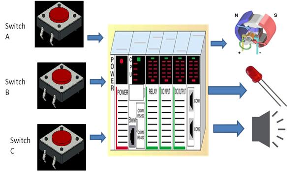
PLC Internal Architecture

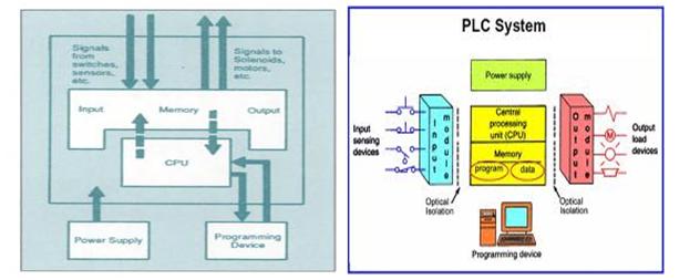
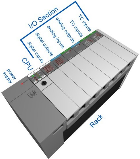
A basic PLC system consists of the following sections:

• Input/ Output Section: The input section or input module consists of devices like sensors, switches and many other real world input sources. The input from the sources is connected to the PLC through the input connector rails. The output section or output module can be a motor or a solenoid or a lamp or a heater, whose functioning is controlled by varying the input signals.
• CPU or Central Processing Unit: It is the brain of the PLC. It can be a hexagonal or an octal microprocessor. It carries out all the processing related to the input signals in order to control the output signals based on the control program.
• Programming Device: It is the platform where the program or the control logic is written. It can be a handheld device or a laptop or a computer itself.
• Power Supply: It generally works on a power supply of about 24 V, used to power input and output devices.
• Memory: The memory is divided into two parts- The data memory and the program memory. The program information or the control logic is stored in the user memory or the program memory from where the CPU fetches the program instructions. The input and output signals and the timer and counter signals are stored in the input and output external image memory respectively.

Working of a PLC

PLC Working Schematic by Edgefx Kits

Working of PLC by Edgefx Kits

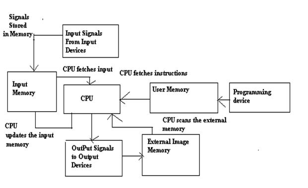
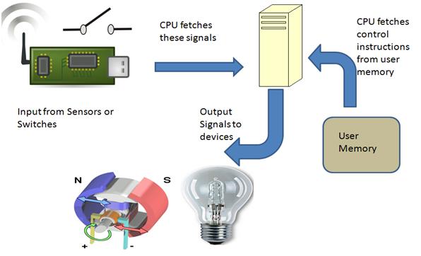
• The input sources convert the real time analog electric signals to suitable digital electric signals and these signals are applied to the PLC through the connector rails.
• These input signals are stored in the PLC external image memory in locations known as bits. This is done by the CPU
• The control logic or the program instructions are written onto the programming device through symbols or through mnemonics and stored in the user memory.
• The CPU fetches these instructions from the user memory and executes the input signals by manipulating, computing, processing them to control the output devices.
• The execution results are then stored in the external image memory which controls the output drives.
• The CPU also keeps a check on the output signals and keeps updating the contents of the input image memory according to the changes in the output memory.
• The CPU also performs internal programming functioning like setting and resetting of the timer, checking the user memory.

Programming in PLC

The basic functioning of the PLC relies on the control logic or the programming technique used. Programming can be done using flowcharts or using ladder logic or using statement logics or mnemonics.

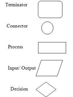
Interlinking all these, let us see how we can actually write a program in PLC.

• Compute the flowchart. A flowchart is the symbolic representation of the instructions. It is the most basic and simplest form of control logic which involves only logic decisions. Different symbols are as given below:

• Write the Boolean expression for the different logic. Boolean algebra usually involves logic operations like AND, OR, NOT, NAND and NOR. The different symbols are:

+   OR operator
.     AND operator
!     NOT operator.

• Write the instructions in simple statement forms like below:

IF Input1 AND Input2 Then SET Output1 ELSE SET Output

 

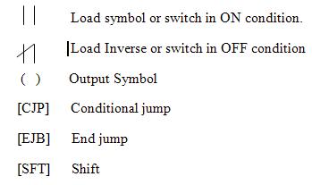
• Write the ladder logic program. It is the most important part of PLC programming. Before explaining about ladder logic programming, let us know about few symbols and terminologies

Rung: One step in the ladder is called a rung. In simpler words, the basic statement or one control logic is called a Rung.
Y- Normal Output signals
M – Motor symbol

T – Timer
C – Counter
Symbols:

Basic Logic Functions using Ladder Logic

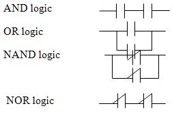
• Writing Mnemonics: Mnemonics are instructions written in symbolic form. They are also known as Opcode and are used in handheld programming devices. Different Symbols are as given below:

Ldi – Load Inverse
Ld- Load
AND- And logic
OR- Or logic
ANI – NAND logic
ORI- NOR logic
Out – Output

A Simple PLC Application

So, now that we have had a brief idea about programming in PLC, lets get into developing one simple application.

Problem: Design a simple line follower robotic system to start a motor when a switch is on and simultaneously switch on the LED.  The sensor on the motor detects any obstacle and another switch is on to indicate the presence of the obstacle and the motor is simultaneously switched off and the buzzer is switched on and LED is off.

Solution:

Solution by Edgefx Kits

Let us first assign our symbols or tags to the inputs and outputs
M – Motor  ,
A – Input Switch 1  ,
B- Input Switch 2 ,
L – LED ,
Bu –Buzzer
Now let us design the Flow Chart

Flowchart for the Design by Edgefx Kits

Next Step is writing the Boolean expressions
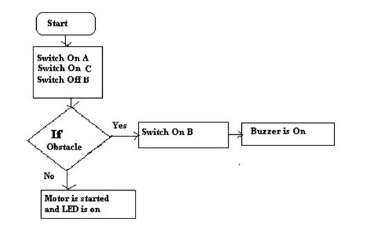
M = A. (! B)
L = C. (! B)
Bu = B. (! A.! C)
The next step involves drawing the ladder logic program

Ladder Logic Program

The final step involves writing the mnemonics to be fed to the handheld device
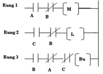
Ld A ANI Ldi B
Ld C ANI Ldi B
Ld B ANI Ldi A AND Ldi C
So, now that I have demonstrated the basic control function using PLC, do let me know more about the ideas of control designs using PLC.



                                      X  .  II  Knowing the basics of PLCs 

Programmable logic controllers provide dependable, high-speed control and monitoring demanded by a wide variety of automated applications.

Programmable logic controllers(PLCs) have gained a substantial hold in the industrial manufacturing arena, and we would be remiss if this technology were not given the due attention it has earned. As such, we are featuring a series of articles based on the fundamentals of PLCs in this new EC&M department covering the technology of solid-state industrial automation. Throughout this series on PLC fundamentals, we'll cover PLC hardware modules; software capabilities; current applications; installation parameters; testing and troubleshooting; and hardware/software maintenance.
What is a PLC?
The National Electrical Manufacturers Association (NEMA) defines a PLC as a "digitally operating electronic apparatus which uses a programmable memory for the internal storage of instructions by implementing specific functions, such as logic, sequencing, timing, counting, and arithmetic to control through digital or analog I/O modules various types of machines or processes."
One PLC manufacturer defines it

as a "solid-state industrial control device which receives signals from user supplied controlled devices, such as senors and switches, implements them in a precise pattern determined by ladder-diagram-based application progress stored in user memory, and provides outputs for control of processes or user-supplied devices, such as relays or motor starters."

Basically, it's a solid-state, programmable electrical/electronic interface that can manipulate, execute, and/or monitor, at a very fast rate, the state of a process or communication system. It operates on the basis of programmable data contained in an integral microprocessor-based system.

 

A PLC is able to receive (input) and transmit (output) various types of electrical and electronic signals and can control and monitor practically any kind of mechanical and/or electrical system. Therefore, it has enormous flexibility in interfacing with computers, machines, and many other peripheral systems or devices.
It's usually programmed in relay ladder logic and is designed to operate in an industrial environment.
What's it look like?
PLCs come in various sizes. Generally, the space or size that a PLC occupies is in direct relation to the user systems and input/output requirements as well as the chosen manufacturer's design/packaging capabilities.
The chassis of a PLC may be of the open or enclosed type. The individual modules plug into the back plane of the chassis.
The electronic components are mounted on printed circuit boards (PCBs) that are contained within a module.
Where did it come from?
The first PLC was introduced in the late 1960s and was an outgrowth of the programmable controller or PC (not to be confused with the notation as used for the personal computer). PCs have been around the industry since the early 60s.
The need for better and faster control relays that fit into less space as well as the frustration over program inflexibility (hard-wired relays, stepping switches, and drum programmers) gave birth to the PC.
Although the PC and PLC have been interchanged in speech, the difference between them is that a PC is dedicated to control functions in a fixed program, similar in a sense to the past problem of limited ability. A PLC, on the other hand, only requires that its software logic be rewritten to meet any new demands of the system being controlled. Thus, a PLC can adapt to changes in many processes or monitoring application requirements.
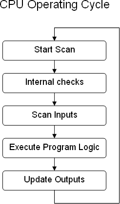
How does a PLC work?
To know how the PLC works, it is essential that we have an understanding of its central processing unit's (CPU's) scan sequence. The methodology basically is the same for all PLCs. However, as special hardware modules are added into the system, additional scanning cycles are required.

Here's one simple scanning process that involves every PLC. First, the I/O hardware modules are scanned by the ladder logic software program as follows.
Upon power-up, the processor scans the input module and transfers the data contents to the input's image table or register. Data from the output image table is transferred to the output module.
Next, the software program is scanned, and each statement is checked to see if the condition has been met. If the conditions are met, the processor writes a digital bit "1" into the output image table, and a peripheral device will be energized. If the conditions are not met, the processor writes a "0" into the output image table, and a peripheral device (using "positive logic") remains deenergized.
A PLC interfaces numerous types of external electrical and electronic signals. These signals can be AC or DC currents or voltages. Typically, they range from 4 to 20 milliamperes (mA) or 0 to 120VAC, and 0 to 48VDC. These signals are referred to as I/O (input/output) points. Their total is called the PLC's I/O capability. From an electronic point-of-view, this number is based on how many points the PLC's CPU is able to look at, or scan, in a specified amount of time. This performance characteristic is called scan time. From the practical perspective of the user, however, the number of I/O modules needed as well as the number of I/O points contained on each I/O module will drive what the system's I/O capability should be.
It's important to have sufficient I/O capability in your PLC system. It's better to have more than less so that, when more I/O points are required at a future time, it's easier to write the existing spare I/O points into the software (since the hardware is already there). There's no harm to the operating system in having spare I/O points; the software can be programmed to ignore them, and these points will have a negligible effect on the PLC's scan time.

The PLC's software program
The software program is the heart of a PLC and is written by a programmer who uses elements, functions, and instructions to design the system that the PLC is to control or monitor. These elements are placed on individually numbered rungs in the relay ladder logic (RLL). The software's RLL is executed by the processor in the CPU module or controller module (same module, different name).
There are many types of PLC software design packages available. One frequently selected software package is of the RLL format and includes contacts, coils, timers, counters, registers, digital comparison blocks, and other types of special data handling functions. Using these elements, the programmer designs the control system. The external devices and components are then wired into the system identical to that of the programmer's software ladder logic. Not all of the software elements will have a hard-wired, physical counterpart, however.
As the PLC's processor scans (topdown) through the software program (rung-by-rung), each rung of RLL is executed. The hard-wired device that the software is mirroring then becomes active. The software is thus the controlling device and provides the programmer or technician the flexibility to either "force a state" or "block a device" from the system operation. For example, a coil or contact can be made to operate directly from the software (independent of the control cabinet's hard-wiring to source or field input devices). Or, a device can be made to appear invisible (removed from the system's operation), even though it's electrically hard-wired and physically in place.
Individual PLC sections
Common to all PLCs are four sections, each of which can be subdivided into smaller but equally important sections. These primary sections include the power supply section, which provides the operating DC power to the PLC and I/O base modules and includes battery backup; the program software section; the CPU module, which contains the processor and holds the memory; and the I/O section, which controls peripheral devices and contains the input and output modules.
Power supply section. The power supply (PS) section gets its input power from an external 120VAC or 240VAC source (line voltage), which is usually fused and fed through a control relay and filter external to the PS. In addition, the PS has its own integral AC input fuse.
This line voltage is then stepped-down, rectified, filtered, regulated, voltage- and current-protected, and status-monitored, with status indication displayed on the front of the PS in the form of several LEDs (light-emitting diodes). The PS can have a key switch for protecting the memory or selecting a particular programming mode.
The output of the PS provides low DC voltage(s) to the PLC's various modules (typically, with a total current capability of 20A or 50A) as well as to its integral lithium battery, which is used for the memory backup. Should the PS fail or its input line voltage drop below a specific value, the memory contents will not change from what they were prior to the failure.
The PS output provides power to every module in the PLC; however, it does not provide the DC voltages to the PLC's peripheral I/O devices.
CPU module. "CPU," "controller," or "processor" are all terms used by different manufacturers to denote the same module that performs basically the same functions. The CPU module can be divided into two sections: the processor section and the memory section.
The processor section makes the decisions needed by the PLC so that it can operate and communicate with other modules. It communicates along either a serial or parallel data-bus. An I/O base interface module or individual on-board interface I/O circuitry provides the signal conditioning required to communicate with the processor. The processor section also executes the programmer's RLL software program.
The memory section stores (electronically) retrievable digital information in three dedicated locations of the memory. These memory locations are routinely scanned by the processor. The memory will receive ("write" mode) digital information or have digital information accessed ("read" mode) by the processor. This read/write (R/W) capability provides an easy way to make program changes.
The memory contains data for several types of information. Usually, the data tables, or image registers, and the software program RLL are in the CPU module's memory. The program messages may or may not be resident with the other memory data.
A battery backup is used by some manufacturers to protect the memory contents from being lost should there be a power or memory module failure. Still others use various integrated circuit (IC) memory technologies and design schemes that will protect the memory contents without the use of a battery backup.
A typical memory section of the CPU module has a memory size of 96,000 (96K) bytes. This size tells us how many locations are available in the memory for storage. Additional memory modules can be added to your PLC system as the need arises for greater memory size. These expansion modules are added to the PLC system as the quantity of I/O modules are added or the software program becomes larger. When this is done, the memory size can be as high as 1,024,000 (1024K) bytes.
Manufacturers will state memory size in either "bytes" or "words." A byte is eight bits, and a bit is the smallest digit in the binary code. It's either a logic "1" or a logic "0." A word is equal in length to two bytes or 16 bits. Not all manufacturers use 16-bit words, so be aware of what your PLC manufacturer has defined as its memory word bit size.
Software program. The PLC not only requires electronic components to operate, it also needs a software program. The PLC programmer is not limited to writing software in one format. There are many types available, each lending itself more readily to one application over and above another. Typical is the RLL type previously discussed. Other S/W programs include "C," State Language, and SFC (Sequential Function Charts).
Regardless of which software is chosen, it will be executed by the PLC's CPU module. The software can be written and executed with the processor in an online state (while the PLC is actually running) or in the off-line state (whereby the S/W execution does not affect current operation of the I/O base).
In the RLL software program, we find several types of programming elements and functions to control processes both internal to the PLC (memory and register) as well as external (field) devices. Listed below are some of the more common types of elements, functions, and instructions:
* Contacts (can be either normally opened or closed; highlighted on the monitor means they are active).
* Coils (can be normal or latched; highlighted means they are energized).
* Timers (coil can either be ON or OFF for the specified delay).
* Counters (can count by increments either up or down).
* Bit shift registers (can shift data by one bit when active).
* One-shot (meaning active for one scan time; useful for pulse timer).
* Drums (can be sequenced based on a time or event).
* Data manipulation instructions (enable movement, comparison of digital values).
* Arithmetic instructions (enable addition, subtraction, multiplication, and division of digital values).
Peripheral devices
Peripheral devices to the PLC and its I/O base(s) can be anything from a host computer and control console to a motor drive unit or field limit switch. Printers and industrial terminals used for programming are also peripheral devices.
Peripheral devices can generate or receive AC or DC voltages and currents as well as digital pulse trains or single pulses of quick length (pulse width).
These external operating devices, with their sometimes harsh and/or fast signal characteristics, must be able to interface with the PLC's sensitive microprocessor. Various types of I/O modules (using the proper shielded cabling) are available to do this job.
Input module
The input module has two functions: reception of an external signal and status display of that input point. In other words, it receives the peripheral sensing unit's signal and provides signal conditioning, termination, isolation and/or indication for that signal's state.
The input to an input module is in either a discrete or analog form. If the input is an ON-OFF type, such as with a push button or limit switch, the signal is considered to be of a discrete nature. If, on the other hand, the input varies, such as with temperature, pressure, or level, the signal is analog in nature.
Peripheral devices sending signals to input modules that describe external conditions can be switches (limit, proximity, pressure, or temperature), push buttons, or logic, binary coded decimal (BCD) or analog-to-digital (A/D) circuits. These input signal points are scanned, and their status is communicated through the interface module or circuitry within each individual PLC and I/O base. Some typical types of input modules are listed below.
* DC voltage (110, 220, 14, 24, 48, 15-30V) or current (4-20 mA).
* AC voltage (110, 240, 24, 48V) or current (4-20 mA).
* TTL (transistor transistor logic) input (3-15VDC).
* Analog input (12-bit).
* Word input (16-bit/parallel).
* Thermocouple input.
* Resistance temperature detector.
* High current relay.
* Low current relay.
* Latching input (24VDC/110VAC).
* Isolated input (24VDC/85-132VAC).
* Intelligent input (contains a microprocessor).
* Positioning input.
* PID (proportional, intregal, differentiation) input.
* High-speed pulse.
Output module
The output module transmits discrete or analog signals to activate various devices such as hydraulic actuators, solenoids, motor starters, and displays the status (through the use of LEDs) of the connected output points. Signal conditioning, termination, and isolation are also part of the output module's functions. The output module is treated in the same manner as the input module by the processor.
Some typical output modules available today include the following:
* DC voltage (24, 48,110V) or current (4-20 mA).
* AC voltage (110, 240v) or current (4-20 mA).
* Isolated (24VDC).
* Analog output (12-bit).
* Word output (16-bit/parallel).
* Intelligent output.
* ASCII output.
* Dual communication port.
TERMS TO KNOW
A/D: A device or module that transforms an analog signal into a digital word.
Address: A numbered location (storage number) in the PLC's memory to store information.
Analog input: A varying signal supplying process change information to the analog input module.
Analog output: A varying signal transmitting process change information from the analog output module.
Baud rate: The number of bits per second that is either transmitted or received; also the speed of digital transmission acceptable by a device.
BCD: Binary coded decimal. A method used to express the 0-thru-9 (base 10) numbering system as a binary (base 2) equivalent.
Bit: A single binary digit.
Byte: Eight bits.
Central Processing Unit (CPU): An integrated circuit (IC) that interprets, decides, and executes instructions.
D/A: A device or module that transforms a digital word into an analog signal
Electrically Erasable Programmable Read-Only Memory (EEPROM): Same as EPROM but can be erased electrically.
Erasable Programmable Read-Only Memory (EPROM): A memory that a user can erase and load with new data many times, but when used in application, it functions as a ROM. EPROMs will not lose data during the loss of electrical power. They are nonvolatile memories.
Image register/image table: A dedicated memory location reserved for I/O bit status.
Input module: Processes digital or analog signals from field devices.
I/O points: Terminal points on I/O modules that connect the input and output field devices.
Millisecond: One thousandth of a second (1/1000 sec, 0.001 sec).
Modem: Modem is an acronym for modulator/demodulator. This is a device that modulates (mixes) and demodulates (separates) signals.
Operator interface: Devices that allow the system operators to have access to PLC and I/O base conditions.
Output module: Controls field devices.
Parallel data: Data whose bytes or words are transmitted or received with all their bits present at the same time.
Program: One or more instructions or statements that accomplish a task.
Programming device: A device used to tell a PLC what to do and when it should be done.
Random Access Memory (RAM): A memory where data can be accessed at any address without having to read a number of sequential addresses. Data can be read from and written to storage locations. RAM has volatile memory, meaning a loss of power will cause the contents in the RAM to be lost.
Read-Only Memory (ROM): A memory from which data can be read but not written. ROMs are often used to keep programs or data from being destroyed due to user intervention.
Software: One or more programs that control a process.
\




                                                   X  .  III  How PLCs Work


A programmable logic controller is a specialized computer used to control machines and processes.  It therefore shares common terms with typical PCs like central processing unit, memory, software and communications.  Unlike a personal computer though the PLC is designed to survive in a rugged industrial atmosphere and to be very flexible in how it interfaces with inputs and outputs to the real world.
The components that make a PLC work can be divided into three core areas.

• The power supply and rack
• The central processing unit (CPU)
• The input/output (I/O) section

PLCs come in many shapes and sizes.  They can be so small as to fit in your shirt pocket while more involved controls systems require large PLC racks.  Smaller PLCs (a.k.a. “bricks”) are typically designed with fixed I/O points.  For our consideration, we’ll look at the more modular rack based systems.  It’s called “modular” because the rack can accept many different types of I/O modules that simply slide into the rack and plug in.

The Power Supply and Rack

So let’s start off by removing all our modules which leaves us with a naked PLC with only the power supply and the rack.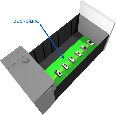

 
The rack is the component that holds everything together.  Depending on the needs of the control system it can be ordered in different sizes to hold more modules.  Like a human spine the rack has a backplane at the rear which allows the cards to communicate with the CPU.  The power supply plugs into the rack as well and supplies a regulated DC power to other modules that plug into the rack.  The most popular power supplies work with 120 VAC or 24 VDC sources.

The CPU

The brain of the whole PLC is the CPU module.  This module typically lives in the slot beside the power supply.  Manufacturers offer different types of CPUs based on the complexity needed for the system.
The CPU consists of a microprocessor, memory chip and other integrated circuits to control logic, monitoring and communications.  The CPU has different operating modes.  In programming mode it accepts the downloaded logic from a PC.  The CPU is then placed in run mode so that it can execute the program and operate the process.

 
Since a PLC is a dedicated controller it will only process this one program over and over again.  One cycle through the program is called a scan time and involves reading the inputs from the other modules, executing the logic based on these inputs and then updated the outputs accordingly.  The scan time happens very quickly (in the range of 1/1000th of a second).  The memory in the CPU stores the program while also holding the status of the I/O and providing a means to store values.

 

I/O System

The I/O system provides the physical connection between the equipment and the PLC.  Opening the doors on an I/O card reveals a terminal strip where the devices connect.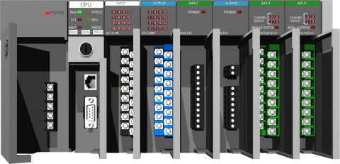

 
There are many different kinds of I/O cards which serve to condition the type of input or output so the CPU can use it for it’s logic.  It's simply a matter of determining what inputs and outputs are needed, filling the rack with the appropriate cards and then addressing them correctly in the CPUs program.

 
Inputs
Input devices can consist of digital or analog devices.  A digital input card handles discrete devices which give a signal that is either on or off such as a pushbutton, limit switch, sensors or selector switches.  An analog input card converts a voltage or current (e.g. a signal that can be anywhere from 0 to 20mA) into a digitally equivalent number that can be understood by the CPU.  Examples of analog devices are pressure transducers, flow meters and thermocouples for temperature readings
Outputs
Output devices can also consist of digital or analog types.  A digital output card either turns a device on or off such as lights, LEDs, small motors, and relays.  An analog output card will convert a digital number sent by the CPU to it’s real world voltage or current.  Typical outputs signals can range from 0-10 VDC or 4-20mA and are used to drive mass flow controllers, pressure regulators and position controls.

Programming a PLC

In these modern times a PC with specially dedicated software from the PLC manufacturer is used to program a PLC.  The most widely used form of programming is called ladder logic.  Ladder logic uses symbols, instead of words, to emulate the real world relay logic control, which is a relic from the PLC's history.  These symbols are interconnected by lines to indicate the flow of current through relay like contacts and coils.  Over the years the number of symbols has increased to provide a high level of functionality. 
The completed program looks like a ladder but in actuality it represents an electrical circuit.  The left and right rails indicate the positive and ground of a power supply.  The rungs represent the wiring between the different components which in the case of a PLC are all in the virtual world of the CPU.  So if you can understand how basic electrical circuits work then you can understand ladder logic.
In this simplest of examples a digital input (like a button connected to the first position on the card) when it is pressed turns on an output which energizes an indicator light.

 
The completed program is downloaded from the PC to the PLC using a special cable that’s connected to the front of the CPU.  The CPU is then put into run mode so that it can start scanning the logic and controlling the outputs.

A Programmable Logic Controller is a device that a user can program to perform a series or sequence of events. These events are triggered by stimuli (called inputs) received at the programmable logic controller through delayed actions such as time delays or counted occurrences.

Once an event triggers, it actuates in the outside world by switching on or off electronic control gear or the physical actuation of devices. A Programmable Logic Controllers will continually loop through its user defined program waiting for inputs and giving outputs at the specific programmed times.

As you would imagine in the world of computers they have their own language. This language is used to program the Programmable Logic Controller can be used in three formats, ladder, instruction list and logic symbol. More about this a bit later on.

Programmable Logic Controllers first came about as a replacement for automatic control systems that used tens and hundreds (maybe even thousands) of hard wired relays, motor driven cam timers and rotary sequencers.

More often then not, a single PLC can be programmed to replace thousands of relays and timers. These Programmable Logic Controllers were first befriended by the automotive manufacturing industry, this enabled software revision to replace the laborious re-wiring of control panels when a new production model was introduced.

Many of the earliest Programmable Logic Controllers expressed all decision making logic in a program format called Ladder Logic, which from its appearance was very similar to electrical schematic diagrams.

This of course was perfect for the electricians of the day, whom quite able to follow and trace out circuit problems with electrical schematic diagrams.

So using ladder logic became second nature to them allowing the electricians an relatively easy transition from hard wired circuits to software driven circuits.

This is the reason this program notation was chosen, to reduce training time for the existing technicians. Other early Programmable Logic Controllers used an instruction list type form of programming, based on a stack-based logic solver. Which was far most difficult to master.

So, what’s a Program?

I’m glad to description the program ;

A program is a connected series of instructions written in a language that the Programmable Logic Controller can understand. There are three forms of program format for PLC’s these are Ladder, Instruction and SFC/STL. Not all programming tools can work with all programming formats.

Generally hand held programming panels only work with instruction format while most graphic programming tools work with both instruction and ladder format. Specialist programming software will also allow SFC style programming but that’s for another time.

We will only be concerning ourselves with Ladder Logic programming here, because it's the most widespread in use today, probably because it's the easiest to grasp and get into the quickest.

Now, there's one big difference between a PLC and a PC type computer; as mentioned above, they only have one program to run. Unlike the PC, which is capable of running several programs at once within the Windows framework. Any of these could one or many many more of the different programs that could be installed on the PC. Why? In one word, speed.

A PLC will be designed to run its one program at a very fast speed, only branching out from within the main bit when an event happens. Events that happen in real time. This gives our little PLC beastie the ability to respond very quickly to any of the events under its control via an input.

Its response would then be carried out via an output. For example controlling a machines production running at 30,000 units an hour! Such as an offset web printing press churning out newspapers or book pages.

Ladder Logic, (the PLC programming language) is very closely associated to relay logic. In relay logic there are both contacts and coils that can be loaded and driven in different configurations. As there are in ladder logic, but a lot more configurations are possible. However the basic principal remains the same.

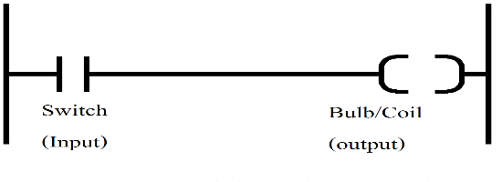
The program is written to switch the desired outputs for a given set of inputs energized. The 'hello world' program equivalent for a PLC would be a light bulb and a switch (see below). The switch is the input and the bulb would be controlled by the output. So, when the switch (input) is on, the bulb (output) is on.

A coil (relay logic terminology) drives outputs of the PLC (a ‘Y’ device, e.g. Y01) or drives internal coils (‘M’ device) timers, counters or flags. Each coil has associated contacts. These contacts are available in both normally open (NO) and normally closed (NC) configurations.

The term normally refers to the status of the contacts when the coil is not energized. Using a relay analogy, when the coil is off, a NO contact would have no current flow, that is, a load being supplied through a NO contact would not operate. However, a NC contact would allow current to flow, hence the connected load would be active.

Activating the coil reverses the contact status, that is, the current would flow in a NO contact and a NC contact would then inhibit the flow.

Physical inputs to the PLC (X devices) have no programmable coil. These devices may only be used in a contact format, again with NO and NC types available.

Because of the close relay logic association, ladder logic programs can be read as current flowing from the left vertical line to the right vertical line. This current must pass through the input (switch) configuration in order to switch the output coil Y0 on.

Therefore in the example below, switching X0 on and X1 being off would causes the output Y0 to also to switch on. However, if X1 were to switch on while X0 was on, the output coil would then switch off.

This is a very basic example of course, as they are very capable of automating a complete warehouse or running very complex machines on their own.

Then, as you would imagine, the program it would be running would have many twists and turns to respond to the 10's and quite possibly even 100's of inputs and outputs. These inputs in conjunction with the program would be dictating the on and off pattern of the outputs at any given time.

Here are just a few examples of Programmable Logic Controller programming applications that have been successfully completed and are in use today.

• Manufacturing Industry
  - Lead acid battery plant, complete manufacturing system
  - Extruder factory, silo feeding control system
• Travel Industry
  - Escalator operation, monitored safety control system
  - Lift operation, monitored safety control system
• Aerospace
  - Water tank quenching system
• Printing Industry
  - Offset web press print register control system
  - Multistage screen washing system
• Food Industry
  - Filling machine control system
  - Main factory feed water pump duty changeover system
• Textile Industry
  - Industrial batch washing machine control system
  - Closed loop textile shrinkage system
• Hospitals
  - Coal fired boiler fan change-over system
• Film Industry
  - Servo axis controlled camera positioning system
• Corrugating
  - Main corrugation machine control system
  - BOBST platten press drive and control system
• Plastics Industry
  - Extruder factory, silo feeding control system
  - Injection moulding control system
• Agriculture
  - Glasshouse heating, ventilation & watering system
• Foundry
  - Overhead transportation system from casting process to shoot blasting machine
• Leisure
  - Roller coaster ride and effects control system
  - Greyhound track 'Rabbit' drive system

As we said these are just a few examples of plc programming applications, there are many many more in use today. In point of fact, there are far too many to list here, the PLC is today's unseen hero controlling a massive range of equipment.

Manufacturers such as Mitsubishi, Allen Bradley, Omron and Siemens have been around for a long time and produce very high quality equipment through years of development (they should be paying me for advertising). It is quite probable that your machines have one of these makes controlling it.

                                X  .  IIII  Programmable Logic Controllers (PLC) 


Before the advent of solid-state logic circuits, logical control systems were designed and built exclusively around electromechanical relays. Relays are far from obsolete in modern design, but have been replaced in many of their former roles as logic-level control devices, relegated most often to those applications demanding high current and/or high voltage switching.
Systems and processes requiring “on/off” control abound in modern commerce and industry, but such control systems are rarely built from either electromechanical relays or discrete logic gates. Instead, digital computers fill the need, which may be programmed to do a variety of logical functions.

In the late 1960’s an American company named Bedford Associates released a computing device they called the MODICON. As an acronym, it meant Modular Digital Controller, and later became the name of a company division devoted to the design, manufacture, and sale of these special-purpose control computers. Other engineering firms developed their own versions of this device, and it eventually came to be known in non-proprietary terms as a PLC, or Programmable Logic Controller. The purpose of a PLC was to directly replace electromechanical relays as logic elements, substituting instead a solid-state digital computer with a stored program, able to emulate the interconnection of many relays to perform certain logical tasks.
A PLC has many “input” terminals, through which it interprets “high” and “low” logical states from sensors and switches. It also has many output terminals, through which it outputs “high” and “low” signals to power lights, solenoids, contactors, small motors, and other devices lending themselves to on/off control. In an effort to make PLCs easy to program, their programming language was designed to resemble ladder logic diagrams. Thus, an industrial electrician or electrical engineer accustomed to reading ladder logic schematics would feel comfortable programming a PLC to perform the same control functions.
PLCs are industrial computers, and as such their input and output signals are typically 120 volts AC, just like the electromechanical control relays they were designed to replace. Although some PLCs have the ability to input and output low-level DC voltage signals of the magnitude used in logic gate circuits, this is the exception and not the rule.
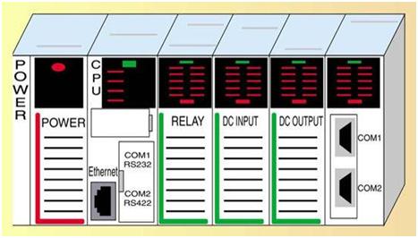
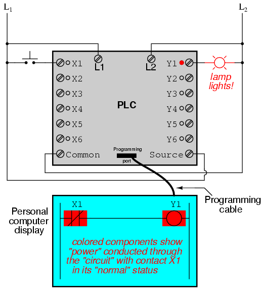
Signal connection and programming standards vary somewhat between different models of PLC, but they are similar enough to allow a “generic” introduction to PLC programming here. The following illustration shows a simple PLC, as it might appear from a front view. Two screw terminals provide connection to 120 volts AC for powering the PLC’s internal circuitry, labeled L1 and L2. Six screw terminals on the left-hand side provide connection to input devices, each terminal representing a different input “channel” with its own “X” label. The lower-left screw terminal is a “Common” connection, which is generally connected to L2 (neutral) of the 120 VAC power source.



Inside the PLC housing, connected between each input terminal and the Common terminal, is an opto-isolator device (Light-Emitting Diode) that provides an electrically isolated “high” logic signal to the computer’s circuitry (a photo-transistor interprets the LED’s light) when there is 120 VAC power applied between the respective input terminal and the Common terminal. An indicating LED on the front panel of the PLC gives visual indication of an “energized” input:



Output signals are generated by the PLC’s computer circuitry activating a switching device (transistor, TRIAC, or even an electromechanical relay), connecting the “Source” terminal to any of the “Y-” labeled output terminals. The “Source” terminal, correspondingly, is usually connected to the L1 side of the 120 VAC power source. As with each input, an indicating LED on the front panel of the PLC gives visual indication of an “energized” output:



In this way, the PLC is able to interface with real-world devices such as switches and solenoids.
The actual logic of the control system is established inside the PLC by means of a computer program. This program dictates which output gets energized under which input conditions. Although the program itself appears to be a ladder logic diagram, with switch and relay symbols, there are no actual switch contacts or relay coils operating inside the PLC to create the logical relationships between input and output. These are imaginary contacts and coils, if you will. The program is entered and viewed via a personal computer connected to the PLC’s programming port.
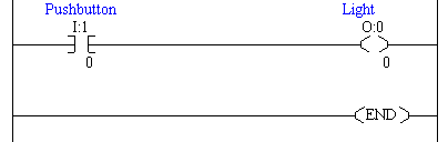
Consider the following circuit and PLC program:



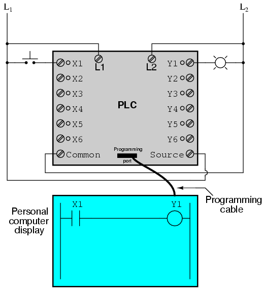
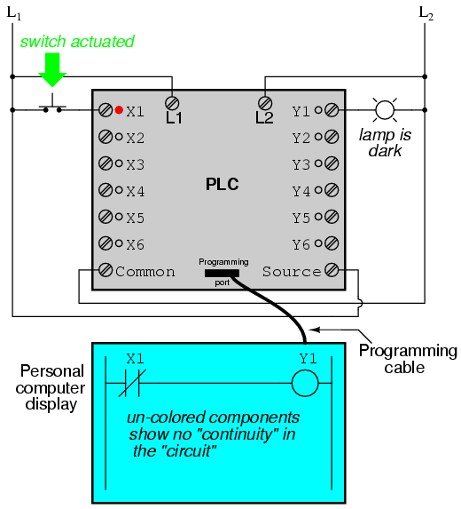
When the pushbutton switch is unactuated (unpressed), no power is sent to the X1 input of the PLC. Following the program, which shows a normally-open X1 contact in series with a Y1 coil, no “power” will be sent to the Y1 coil. Thus, the PLC’s Y1 output remains de-energized, and the indicator lamp connected to it remains dark.
If the pushbutton switch is pressed, however, power will be sent to the PLC’s X1 input. Any and all X1 contacts appearing in the program will assume the actuated (non-normal) state, as though they were relay contacts actuated by the energizing of a relay coil named “X1”. In this case, energizing the X1 input will cause the normally-open X1 contact will “close,” sending “power” to the Y1 coil. When the Y1 coil of the program “energizes,” the real Y1 output will become energized, lighting up the lamp connected to it:



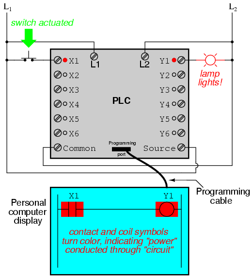
It must be understood that the X1 contact, Y1 coil, connecting wires, and “power” appearing in the personal computer’s display are all virtual. They do not exist as real electrical components. They exist as commands in a computer program—a piece of software only—that just happens to resemble a real relay schematic diagram.
Equally important to understand is that the personal computer used to display and edit the PLC’s program is not necessary for the PLC’s continued operation. Once a program has been loaded to the PLC from the personal computer, the personal computer may be unplugged from the PLC, and the PLC will continue to follow the programmed commands. I include the personal computer display in these illustrations for your sake only, in aiding to understand the relationship between real-life conditions (switch closure and lamp status) and the program’s status (“power” through virtual contacts and virtual coils).
The true power and versatility of a PLC is revealed when we want to alter the behavior of a control system. Since the PLC is a programmable device, we can alter its behavior by changing the commands we give it, without having to reconfigure the electrical components connected to it. For example, suppose we wanted to make this switch-and-lamp circuit function in an inverted fashion: push the button to make the lamp turn off, and release it to make it turn on. The “hardware” solution would require that a normally-closed pushbutton switch be substituted for the normally-open switch currently in place. The “software” solution is much easier: just alter the program so that contact X1 is normally-closed rather than normally-open.
In the following illustration, we have the altered system shown in the state where the pushbutton is unactuated (not being pressed):



In this next illustration, the switch is shown actuated (pressed):



One of the advantages of implementing logical control in software rather than in hardware is that input signals can be re-used as many times in the program as is necessary. For example, take the following circuit and program, designed to energize the lamp if at least two of the three pushbutton switches are simultaneously actuated:



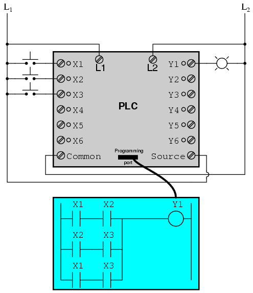
To build an equivalent circuit using electromechanical relays, three relays with two normally-open contacts each would have to be used, to provide two contacts per input switch. Using a PLC, however, we can program as many contacts as we wish for each “X” input without adding additional hardware, since each input and each output is nothing more than a single bit in the PLC’s digital memory (either 0 or 1), and can be recalled as many times as necessary.
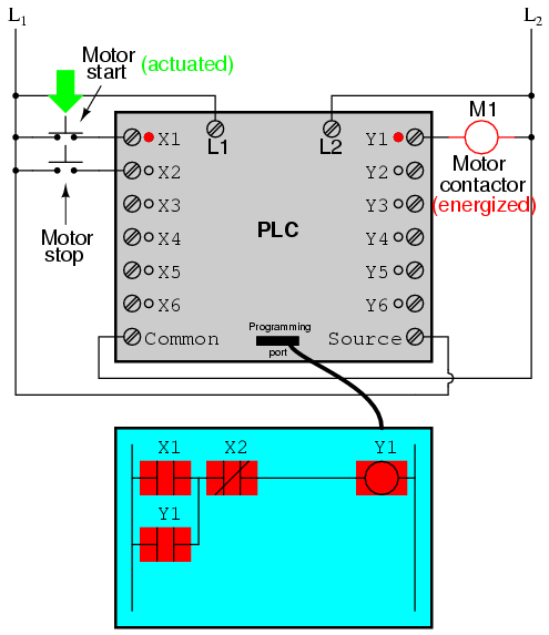
Furthermore, since each output in the PLC is nothing more than a bit in its memory as well, we can assign contacts in a PLC program “actuated” by an output (Y) status. Take for instance this next system, a motor start-stop control circuit:




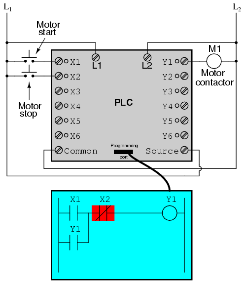
The pushbutton switch connected to input X1 serves as the “Start” switch, while the switch connected to input X2 serves as the “Stop.” Another contact in the program, named Y1, uses the output coil status as a seal-in contact, directly, so that the motor contactor will continue to be energized after the “Start” pushbutton switch is released. You can see the normally-closed contact X2 appear in a colored block, showing that it is in a closed (“electrically conducting”) state.
If we were to press the “Start” button, input X1 would energize, thus “closing” the X1 contact in the program, sending “power” to the Y1 “coil,” energizing the Y1 output and applying 120 volt AC power to the real motor contactor coil. The parallel Y1 contact will also “close,” thus latching the “circuit” in an energized state:



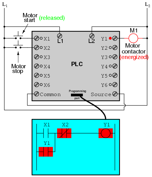
Now, if we release the “Start” pushbutton, the normally-open X1 “contact” will return to its “open” state, but the motor will continue to run because the Y1 seal-in “contact” continues to provide “continuity” to “power” coil Y1, thus keeping the Y1 output energized:



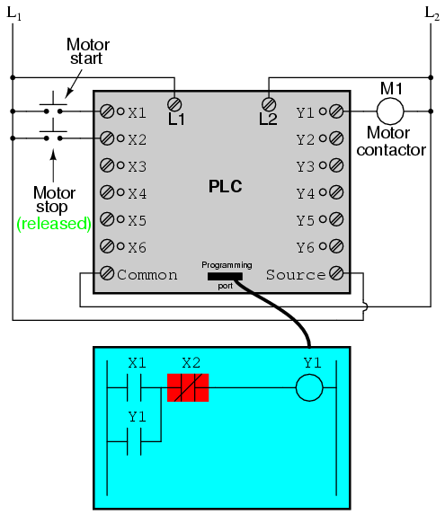
To stop the motor, we must momentarily press the “Stop” pushbutton, which will energize the X2 input and “open” the normally-closed “contact,” breaking continuity to the Y1 “coil:”



When the “Stop” pushbutton is released, input X2 will de-energize, returning “contact” X2 to its normal, “closed” state. The motor, however, will not start again until the “Start” pushbutton is actuated, because the “seal-in” of Y1 has been lost:




An important point to make here is that fail-safe design is just as important in PLC-controlled systems as it is in electromechanical relay-controlled systems. One should always consider the effects of failed (open) wiring on the device or devices being controlled. In this motor control circuit example, we have a problem: if the input wiring for X2 (the “Stop” switch) were to fail open, there would be no way to stop the motor!
The solution to this problem is a reversal of logic between the X2 “contact” inside the PLC program and the actual “Stop” pushbutton switch:



When the normally-closed “Stop” pushbutton switch is unactuated (not pressed), the PLC’s X2 input will be energized, thus “closing” the X2 “contact” inside the program. This allows the motor to be started when input X1 is energized, and allows it to continue to run when the “Start” pushbutton is no longer pressed. When the “Stop” pushbutton is actuated, input X2 will de-energize, thus “opening” the X2 “contact” inside the PLC program and shutting off the motor. So, we see there is no operational difference between this new design and the previous design.
However, if the input wiring on input X2 were to fail open, X2 input would de-energize in the same manner as when the “Stop” pushbutton is pressed. The result, then, for a wiring failure on the X2 input is that the motor will immediately shut off. This is a safer design than the one previously shown, where a “Stop” switch wiring failure would have resulted in an inability to turn off the motor.
In addition to input (X) and output (Y) program elements, PLCs provide “internal” coils and contacts with no intrinsic connection to the outside world. These are used much the same as “control relays” (CR1, CR2, etc.) are used in standard relay circuits: to provide logic signal inversion when necessary.
To demonstrate how one of these “internal” relays might be used, consider the following example circuit and program, designed to emulate the function of a three-input NAND gate. Since PLC program elements are typically designed by single letters, I will call the internal control relay “C1” rather than “CR1” as would be customary in a relay control circuit:



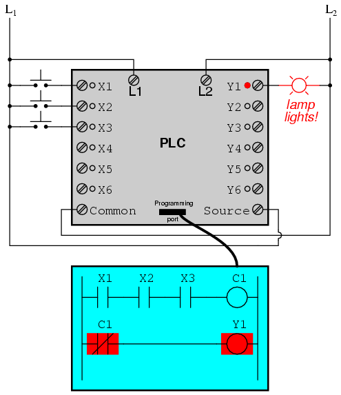
In this circuit, the lamp will remain lit so long as any of the pushbuttons remain unactuated (unpressed). To make the lamp turn off, we will have to actuate (press) all three switches, like this:



This section on programmable logic controllers illustrates just a small sample of their capabilities. As computers, PLCs can perform timing functions (for the equivalent of time-delay relays), drum sequencing, and other advanced functions with far greater accuracy and reliability than what is possible using electromechanical logic devices. Most PLCs have the capacity for far more than six inputs and six outputs. The following photograph shows several input and output modules of a single Allen-Bradley PLC.



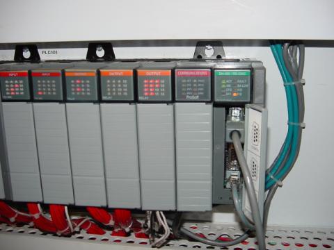
With each module having sixteen “points” of either input or output, this PLC has the ability to monitor and control dozens of devices. Fit into a control cabinet, a PLC takes up little room, especially considering the equivalent space that would be needed by electromechanical relays to perform the same functions:



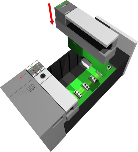
One advantage of PLCs that simply cannot be duplicated by electromechanical relays is remote monitoring and control via digital computer networks. Because a PLC is nothing more than a special-purpose digital computer, it has the ability to communicate with other computers rather easily. The following photograph shows a personal computer displaying a graphic image of a real liquid-level process (a pumping, or “lift,” station for a municipal wastewater treatment system) controlled by a PLC. The actual pumping station is located miles away from the personal computer display:






“Ladder” Diagrams  

Ladder diagrams are specialized schematics commonly used to document industrial control logic systems. They are called “ladder” diagrams because they resemble a ladder, with two vertical rails (supply power) and as many “rungs” (horizontal lines) as there are control circuits to represent. If we wanted to draw a simple ladder diagram showing a lamp that is controlled by a hand switch, it would look like this:




The “L₁” and “L₂” designations refer to the two poles of a 120 VAC supply unless otherwise noted. L₁ is the “hot” conductor, and L₂ is the grounded (“neutral”) conductor. These designations have nothing to do with inductors, just to make things confusing. The actual transformer or generator supplying power to this circuit is omitted for simplicity. In reality, the circuit looks something like this:



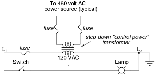
Typically in industrial relay logic circuits, but not always, the operating voltage for the switch contacts and relay coils will be 120 volts AC. Lower voltage AC and even DC systems are sometimes built and documented according to “ladder” diagrams:



So long as the switch contacts and relay coils are all adequately rated, it really doesn’t matter what level of voltage is chosen for the system to operate with.
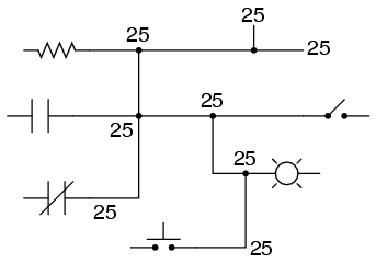
Note the number “1” on the wire between the switch and the lamp. In the real world, that wire would be labeled with that number, using heat-shrink or adhesive tags, wherever it was convenient to identify. Wires leading to the switch would be labeled “L₁” and “1,” respectively. Wires leading to the lamp would be labeled “1” and “L₂,” respectively. These wire numbers make assembly and maintenance very easy. Each conductor has its own unique wire number for the control system that its used in. Wire numbers do not change at any junction or node, even if wire size, color, or length changes going into or out of a connection point. Of course, it is preferable to maintain consistent wire colors, but this is not always practical. What matters is that any one, electrically continuous point in a control circuit possesses the same wire number. Take this circuit section, for example, with wire #25 as a single, electrically continuous point threading to many different devices:



In ladder diagrams, the load device (lamp, relay coil, solenoid coil, etc.) is almost always drawn at the right-hand side of the rung. While it doesn’t matter electrically where the relay coil is located within the rung, it does matter which end of the ladder’s power supply is grounded, for reliable operation.
Take for instance this circuit:



Here, the lamp (load) is located on the right-hand side of the rung, and so is the ground connection for the power source. This is no accident or coincidence; rather, it is a purposeful element of good design practice. Suppose that wire #1 were to accidentally come in contact with ground, the insulation of that wire having been rubbed off so that the bare conductor came in contact with grounded, metal conduit. Our circuit would now function like this:



With both sides of the lamp connected to ground, the lamp will be “shorted out” and unable to receive power to light up. If the switch were to close, there would be a short-circuit, immediately blowing the fuse.
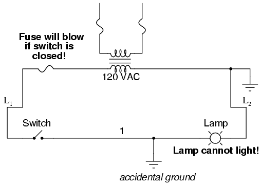
However, consider what would happen to the circuit with the same fault (wire #1 coming in contact with ground), except this time we’ll swap the positions of switch and fuse (L₂ is still grounded):



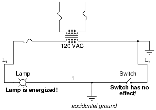
This time the accidental grounding of wire #1 will force power to the lamp while the switch will have no effect. It is much safer to have a system that blows a fuse in the event of a ground fault than to have a system that uncontrollably energizes lamps, relays, or solenoids in the event of the same fault. For this reason, the load(s) must always be located nearest the grounded power conductor in the ladder diagram.

• REVIEW:
• Ladder diagrams (sometimes called “ladder logic”) are a type of electrical notation and symbology frequently used to illustrate how electromechanical switches and relays are interconnected.
• The two vertical lines are called “rails” and attach to opposite poles of a power supply, usually 120 volts AC. L₁ designates the “hot” AC wire and L₂ the “neutral” (grounded) conductor.
• Horizontal lines in a ladder diagram are called “rungs,” each one representing a unique parallel circuit branch between the poles of the power supply.
• Typically, wires in control systems are marked with numbers and/or letters for identification. The rule is, all permanently connected (electrically common) points must bear the same label.

Digital Logic Functions

We can construct simple logic functions for our hypothetical lamp circuit, using multiple contacts, and document these circuits quite easily and understandably with additional rungs to our original “ladder.” If we use standard binary notation for the status of the switches and lamp (0 for unactuated or de-energized; 1 for actuated or energized), a truth table can be made to show how the logic works:



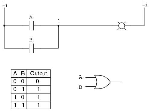
Now, the lamp will come on if either contact A or contact B is actuated, because all it takes for the lamp to be energized is to have at least one path for current from wire L₁ to wire 1. What we have is a simple OR logic function, implemented with nothing more than contacts and a lamp.
We can mimic the AND logic function by wiring the two contacts in series instead of parallel:



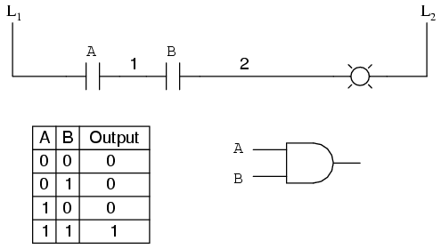
Now, the lamp energizes only if contact A and contact B are simultaneously actuated. A path exists for current from wire L₁ to the lamp (wire 2) if and only if both switch contacts are closed.
The logical inversion, or NOT, function can be performed on a contact input simply by using a normally-closed contact instead of a normally-open contact:



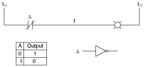
Now, the lamp energizes if the contact is not actuated, and de-energizes when the contact is actuated.

If we take our OR function and invert each “input” through the use of normally-closed contacts, we will end up with a NAND function. In a special branch of mathematics known as Boolean algebra, this effect of gate function identity changing with the inversion of input signals is described by DeMorgan’s Theorem, a subject to be explored in more detail in a later chapter.



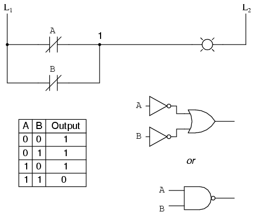
The lamp will be energized if either contact is unactuated. It will go out only if both contacts are actuated simultaneously.
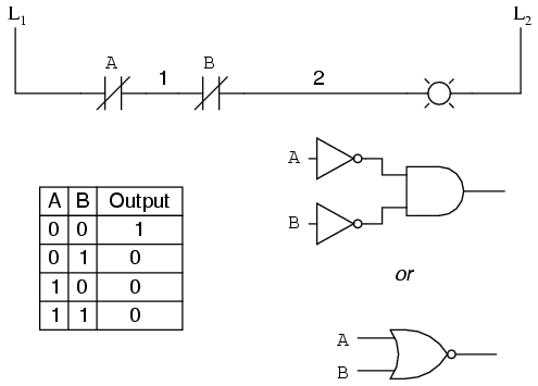
Likewise, if we take our AND function and invert each “input” through the use of normally-closed contacts, we will end up with a NOR function:




A pattern quickly reveals itself when ladder circuits are compared with their logic gate counterparts:

• Parallel contacts are equivalent to an OR gate.
• Series contacts are equivalent to an AND gate.
• Normally-closed contacts are equivalent to a NOT gate (inverter).

We can build combinational logic functions by grouping contacts in series-parallel arrangements, as well. In the following example, we have an Exclusive-OR function built from a combination of AND, OR, and inverter (NOT) gates:



The top rung (NC contact A in series with NO contact B) is the equivalent of the top NOT/AND gate combination. The bottom rung (NO contact A in series with NC contact B) is the equivalent of the bottom NOT/AND gate combination. The parallel connection between the two rungs at wire number 2 forms the equivalent of the OR gate, in allowing either rung 1 or rung 2 to energize the lamp.
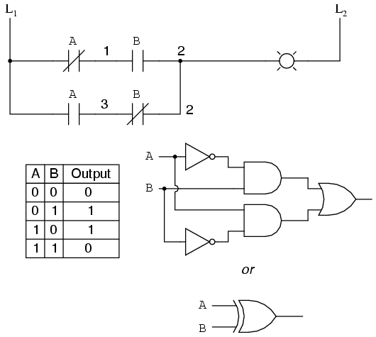
To make the Exclusive-OR function, we had to use two contacts per input: one for direct input and the other for “inverted” input. The two “A” contacts are physically actuated by the same mechanism, as are the two “B” contacts. The common association between contacts is denoted by the label of the contact. There is no limit to how many contacts per switch can be represented in a ladder diagram, as each new contact on any switch or relay (either normally-open or normally-closed) used in the diagram is simply marked with the same label.
Sometimes, multiple contacts on a single switch (or relay) are designated by a compound labels, such as “A-1” and “A-2” instead of two “A” labels. This may be especially useful if you want to specifically designate which set of contacts on each switch or relay is being used for which part of a circuit. For simplicity’s sake, I’ll refrain from such elaborate labeling in this lesson. If you see a common label for multiple contacts, you know those contacts are all actuated by the same mechanism.
If we wish to invert the output of any switch-generated logic function, we must use a relay with a normally-closed contact. For instance, if we want to energize a load based on the inverse, or NOT, of a normally-open contact, we could do this:



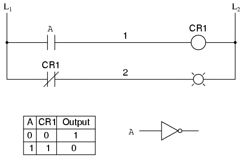
We will call the relay, “control relay 1,” or CR₁. When the coil of CR₁ (symbolized with the pair of parentheses on the first rung) is energized, the contact on the second rung opens, thus de-energizing the lamp. From switch A to the coil of CR₁, the logic function is noninverted. The normally-closed contact actuated by relay coil CR₁ provides a logical inverter function to drive the lamp opposite that of the switch’s actuation status.
Applying this inversion strategy to one of our inverted-input functions created earlier, such as the OR-to-NAND, we can invert the output with a relay to create a noninverted function:



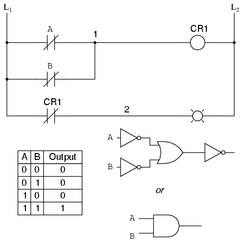
From the switches to the coil of CR₁, the logical function is that of a NAND gate. CR₁‘s normally-closed contact provides one final inversion to turn the NAND function into an AND function.

• REVIEW:
• Parallel contacts are logically equivalent to an OR gate.
• Series contacts are logically equivalent to an AND gate.
• Normally closed (N.C.) contacts are logically equivalent to a NOT gate.
• A relay must be used to invert the output of a logic gate function, while simple normally-closed switch contacts are sufficient to represent inverted gate inputs.

Permissive and Interlock Circuits 

A practical application of switch and relay logic is in control systems where several process conditions have to be met before a piece of equipment is allowed to start. A good example of this is burner control for large combustion furnaces. In order for the burners in a large furnace to be started safely, the control system requests “permission” from several process switches, including high and low fuel pressure, air fan flow check, exhaust stack damper position, access door position, etc. Each process condition is called a permissive, and each permissive switch contact is wired in series, so that if any one of them detects an unsafe condition, the circuit will be opened:



If all permissive conditions are met, CR₁ will energize and the green lamp will be lit. In real life, more than just a green lamp would be energized: usually, a control relay or fuel valve solenoid would be placed in that rung of the circuit to be energized when all the permissive contacts were “good:” that is, all closed. If any one of the permissive conditions are not met, the series string of switch contacts will be broken, CR₂ will de-energize, and the red lamp will light.
Note that the high fuel pressure contact is normally-closed. This is because we want the switch contact to open if the fuel pressure gets too high. Since the “normal” condition of any pressure switch is when zero (low) pressure is being applied to it, and we want this switch to open with excessive (high) pressure, we must choose a switch that is closed in its normal state.
Another practical application of relay logic is in control systems where we want to ensure two incompatible events cannot occur at the same time. An example of this is in reversible motor control, where two motor contactors are wired to switch polarity (or phase sequence) to an electric motor, and we don’t want the forward and reverse contactors energized simultaneously:



When contactor M₁ is energized, the 3 phases (A, B, and C) are connected directly to terminals 1, 2, and 3 of the motor, respectively. However, when contactor M₂ is energized, phases A and B are reversed, A going to motor terminal 2 and B going to motor terminal 1. This reversal of phase wires results in the motor spinning the opposite direction. Let’s examine the control circuit for these two contactors:



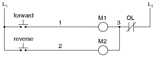
Take note of the normally-closed “OL” contact, which is the thermal overload contact activated by the “heater” elements wired in series with each phase of the AC motor. If the heaters get too hot, the contact will change from its normal (closed) state to being open, which will prevent either contactor from energizing.
This control system will work fine, so long as no one pushes both buttons at the same time. If someone were to do that, phases A and B would be short-circuited together by virtue of the fact that contactor M₁ sends phases A and B straight to the motor and contactor M₂ reverses them; phase A would be shorted to phase B and vice versa. Obviously, this is a bad control system design!

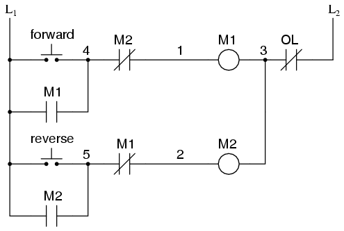
To prevent this occurrence from happening, we can design the circuit so that the energization of one contactor prevents the energization of the other. This is called interlocking, and it is accomplished through the use of auxiliary contacts on each contactor, as such:



Now, when M₁ is energized, the normally-closed auxiliary contact on the second rung will be open, thus preventing M₂ from being energized, even if the “Reverse” pushbutton is actuated. Likewise, M₁‘s energization is prevented when M₂ is energized. Note, as well, how additional wire numbers (4 and 5) were added to reflect the wiring changes.

It should be noted that this is not the only way to interlock contactors to prevent a short-circuit condition. Some contactors come equipped with the option of a mechanical interlock: a lever joining the armatures of two contactors together so that they are physically prevented from simultaneous closure. For additional safety, electrical interlocks may still be used, and due to the simplicity of the circuit there is no good reason not to employ them in addition to mechanical interlocks.

• REVIEW:
• Switch contacts installed in a rung of ladder logic designed to interrupt a circuit if certain physical conditions are not met are called permissive contacts, because the system requires permission from these inputs to activate.
• Switch contacts designed to prevent a control system from taking two incompatible actions at once (such as powering an electric motor forward and backward simultaneously) are called interlocks.

Motor Control Circuits 

The interlock contacts installed in the previous section’s motor control circuit work fine, but the motor will run only as long as each push button switch is held down. If we wanted to keep the motor running even after the operator takes his or her hand off the control switch(es), we could change the circuit in a couple of different ways: we could replace the push button switches with toggle switches, or we could add some more relay logic to “latch” the control circuit with a single, momentary actuation of either switch. Let’s see how the second approach is implemented since it is commonly used in industry:




When the “Forward” pushbutton is actuated, M₁ will energize, closing the normally-open auxiliary contact in parallel with that switch. When the pushbutton is released, the closed M₁ auxiliary contact will maintain current to the coil of M₁, thus latching the “Forward” circuit in the “on” state. The same sort of thing will happen when the “Reverse” pushbutton is pressed. These parallel auxiliary contacts are sometimes referred to as seal-in contacts, the word “seal” meaning essentially the same thing as the word latch.
However, this creates a new problem: how to stop the motor! As the circuit exists right now, the motor will run either forward or backward once the corresponding pushbutton switch is pressed and will continue to run as long as there is power. To stop either circuit (forward or backward), we require some means for the operator to interrupt power to the motor contactors. We’ll call this new switch, Stop:



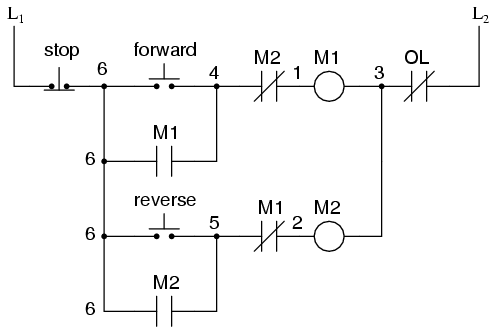
Now, if either forward or reverse circuits are latched, they may be “unlatched” by momentarily pressing the “Stop” pushbutton, which will open either forward or reverse circuit, de-energizing the energized contactor, and returning the seal-in contact to its normal (open) state. The “Stop” switch, having normally-closed contacts, will conduct power to either forward or reverse circuits when released.
So far, so good. Let’s consider another practical aspect of our motor control scheme before we quit adding to it. If our hypothetical motor turned a mechanical load with a lot of momentum, such as a large air fan, the motor might continue to coast for a substantial amount of time after the stop button had been pressed. This could be problematic if an operator were to try to reverse the motor direction without waiting for the fan to stop turning. If the fan was still coasting forward and the “Reverse” pushbutton was pressed, the motor would struggle to overcome that inertia of the large fan as it tried to begin turning in reverse, drawing excessive current and potentially reducing the life of the motor, drive mechanisms, and fan. What we might like to have is some kind of a time-delay function in this motor control system to prevent such a premature startup from happening.
Let’s begin by adding a couple of time-delay relay coils, one in parallel with each motor contactor coil. If we use contacts that delay returning to their normal state, these relays will provide us a “memory” of which direction the motor was last powered to turn. What we want each time-delay contact to do is to open the starting-switch leg of the opposite rotation circuit for several seconds, while the fan coasts to a halt.



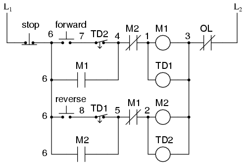
If the motor has been running in the forward direction, both M₁ and TD₁ will have been energized. This being the case, the normally-closed, timed-closed contact of TD₁ between wires 8 and 5 will have immediately opened the moment TD₁ was energized. When the stop button is pressed, contact TD₁ waits for the specified amount of time before returning to its normally-closed state, thus holding the reverse pushbutton circuit open for the duration so M₂ can’t be energized. When TD₁ times out, the contact will close and the circuit will allow M₂ to be energized if the reverse pushbutton is pressed. In like manner, TD₂ will prevent the “Forward” pushbutton from energizing M₁ until the prescribed time delay after M₂ (and TD₂) have been de-energized.
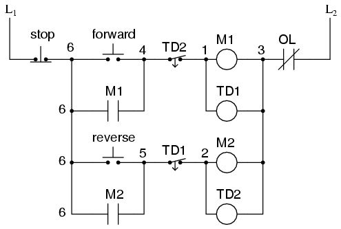
The careful observer will notice that the time-interlocking functions of TD₁ and TD₂ render the M₁ and M₂ interlocking contacts redundant. We can get rid of auxiliary contacts M₁ and M₂ for interlocks and just use TD₁ and TD₂‘s contacts, since they immediately open when their respective relay coils are energized, thus “locking out” one contactor if the other is energized. Each time delay relay will serve a dual purpose: preventing the other contactor from energizing while the motor is running and preventing the same contactor from energizing until a prescribed time after motor shutdown. The resulting circuit has the advantage of being simpler than the previous example:

• REVIEW:
• Motor contactor (or “starter”) coils are typically designated by the letter “M” in ladder logic diagrams.
• Continuous motor operation with a momentary “start” switch is possible if a normally-open “seal-in” contact from the contactor is connected in parallel with the start switch so that once the contactor is energized it maintains power to itself and keeps itself “latched” on.
• Time delay relays are commonly used in large motor control circuits to prevent the motor from being started (or reversed) until a certain amount of time has elapsed from an event.

Fail-safe Design 

Logic circuits, whether comprised of electromechanical relays or solid-state gates, can be built in many different ways to perform the same functions. There is usually no one “correct” way to design a complex logic circuit, but there are usually ways that are better than others.
In control systems, safety is (or at least should be) an important design priority. If there are multiple ways in which a digital control circuit can be designed to perform a task, and one of those ways happens to hold certain advantages in safety over the others, then that design is the better one to choose.
Let’s take a look at a simple system and consider how it might be implemented in relay logic. Suppose that a large laboratory or industrial building is to be equipped with a fire alarm system, activated by any one of several latching switches installed throughout the facility. The system should work so that the alarm siren will energize if any one of the switches is actuated. At first glance, it seems as though the relay logic should be incredibly simple: just use normally-open switch contacts and connect them all in parallel with each other:



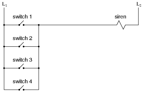
Essentially, this is the OR logic function implemented with four switch inputs. We could expand this circuit to include any number of switch inputs, each new switch being added to the parallel network, but I’ll limit it to four in this example to keep things simple. At any rate, it is an elementary system and there seems to be little possibility of trouble.
Except in the event of a wiring failure, that is. The nature of electric circuits is such that “open” failures (open switch contacts, broken wire connections, open relay coils, blown fuses, etc.) are statistically more likely to occur than any other type of failure. With that in mind, it makes sense to engineer a circuit to be as tolerant as possible to such a failure. Let’s suppose that a wire connection for Switch #2 were to fail open:



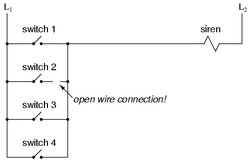
If this failure were to occur, the result would be that Switch #2 would no longer energize the siren if actuated. This, obviously, is not good in a fire alarm system. Unless the system were regularly tested (a good idea anyway), no one would know there was a problem until someone tried to use that switch in an emergency.
What if the system were re-engineered so as to sound the alarm in the event of an open failure? That way, a failure in the wiring would result in a false alarm, a scenario much more preferable than that of having a switch silently fail and not function when needed. In order to achieve this design goal, we would have to re-wire the switches so that an open contact sounded the alarm, rather than a closed contact. That being the case, the switches will have to be normally-closed and in series with each other, powering a relay coil which then activates a normally-closed contact for the siren:



When all switches are unactuated (the regular operating state of this system), relay CR₁ will be energized, thus keeping contact CR₁ open, preventing the siren from being powered. However, if any of the switches are actuated, relay CR₁ will de-energize, closing contact CR₁ and sounding the alarm. Also, if there is a break in the wiring anywhere in the top rung of the circuit, the alarm will sound. When it is discovered that the alarm is false, the workers in the facility will know that something failed in the alarm system and that it needs to be repaired.
Granted, the circuit is more complex than it was before the addition of the control relay, and the system could still fail in the “silent” mode with a broken connection in the bottom rung, but it’s still a safer design than the original circuit, and thus preferable from the standpoint of safety.

This design of circuit is referred to as fail-safe, due to its intended design to default to the safest mode in the event of a common failure such as a broken connection in the switch wiring. Fail-safe design always starts with an assumption as to the most likely kind of wiring or component failure and then tries to configure things so that such a failure will cause the circuit to act in the safest way, the “safest way” being determined by the physical characteristics of the process.
Take for example an electrically-actuated (solenoid) valve for turning on cooling water to a machine. Energizing the solenoid coil will move an armature which then either opens or closes the valve mechanism, depending on what kind of valve we specify. A spring will return the valve to its “normal” position when the solenoid is de-energized. We already know that an open failure in the wiring or solenoid coil is more likely than a short or any other type of failure, so we should design this system to be in its safest mode with the solenoid de-energized.
If it’s cooling water we’re controlling with this valve, chances are it is safer to have the cooling water turn on in the event of a failure than to shut off, the consequences of a machine running without coolant usually being severe. This means we should specify a valve that turns on (opens up) when de-energized and turns off (closes down) when energized. This may seem “backwards” to have the valve set up this way, but it will make for a safer system in the end.
One interesting application of fail-safe design is in the power generation and distribution industry, where large circuit breakers need to be opened and closed by electrical control signals from protective relays. If a 50/51 relay (instantaneous and time overcurrent) is going to command a circuit breaker to trip (open) in the event of excessive current, should we design it so that the relay closes a switch contact to send a “trip” signal to the breaker, or opens a switch contact to interrupt a regularly “on” signal to initiate a breaker trip? We know that an open connection will be the most likely to occur, but what is the safest state of the system: breaker open or breaker closed?
At first, it would seem that it would be safer to have a large circuit breaker trip (open up and shut off power) in the event of an open fault in the protective relay control circuit, just like we had the fire alarm system default to an alarm state with any switch or wiring failure. However, things are not so simple in the world of high power. To have a large circuit breaker indiscriminately trip open is no small matter, especially when customers are depending on the continued supply of electric power to supply hospitals, telecommunications systems, water treatment systems, and other important infrastructures. For this reason, power system engineers have generally agreed to design protective relay circuits to output a closed contact signal (power applied) to open large circuit breakers, meaning that any open failure in the control wiring will go unnoticed, simply leaving the breaker in the status quo position.
Is this an ideal situation? Of course not. If a protective relay detects an overcurrent condition while the control wiring is failed open, it will not be able to trip open the circuit breaker. Like the first fire alarm system design, the “silent” failure will be evident only when the system is needed. However, to engineer the control circuitry the other way—so that any open failure would immediately shut the circuit breaker off, potentially blacking out large potions of the power grid—really isn’t a better alternative.
An entire book could be written on the principles and practices of good fail-safe system design. At least here, you know a couple of the fundamentals: that wiring tends to fail open more often than shorted, and that an electrical control system’s (open) failure mode should be such that it indicates and/or actuates the real-life process in the safest alternative mode. These fundamental principles extend to non-electrical systems as well: identify the most common mode of failure, then engineer the system so that the probable failure mode places the system in the safest condition.

• REVIEW:
• The goal of fail-safe design is to make a control system as tolerant as possible to likely wiring or component failures.
• The most common type of wiring and component failure is an “open” circuit, or broken connection. Therefore, a fail-safe system should be designed to default to its safest mode of operation in the case of an open circuit.

A Binary Adder   Principles Of Digital Computing 


Suppose we wanted to build a device that could add two binary bits together. Such a device is known as a half-adder, and its gate circuit looks like this:



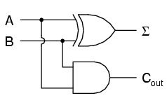
The Σ symbol represents the “sum” output of the half-adder, the sum’s least significant bit (LSB). C_out represents the “carry” output of the half-adder, the sum’s most significant bit (MSB).
If we were to implement this same function in ladder (relay) logic, it would look like this:



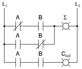
Either circuit is capable of adding two binary digits together. The mathematical “rules” of how to add bits together are intrinsic to the hard-wired logic of the circuits. If we wanted to perform a different arithmetic operation with binary bits, such as multiplication, we would have to construct another circuit. The above circuit designs will only perform one function: add two binary bits together. To make them do something else would take re-wiring, and perhaps different componentry.

In this sense, digital arithmetic circuits aren’t much different from analog arithmetic (operational amplifier) circuits: they do exactly what they’re wired to do, no more and no less. We are not, however, restricted to designing digital computer circuits in this manner. It is possible to embed the mathematical “rules” for any arithmetic operation in the form of digital data rather than in hard-wired connections between gates. The result is unparalleled flexibility in operation, giving rise to a whole new kind of digital device: the programmable computer.
While this chapter is by no means exhaustive, it provides what I believe is a unique and interesting look at the nature of programmable computer devices, starting with two devices often overlooked in introductory textbooks: look-up table memories and finite-state machines.



Look-up Tables  

Having learned about digital memory devices in the last chapter, we know that it is possible to store binary data within solid-state devices. Those storage “cells” within solid-state memory devices are easily addressed by driving the “address” lines of the device with the proper binary value(s). Suppose we had a ROM memory circuit written, or programmed, with certain data, such that the address lines of the ROM served as inputs and the data lines of the ROM served as outputs, generating the characteristic response of a particular logic function. Theoretically, we could program this ROM chip to emulate whatever logic function we wanted without having to alter any wire connections or gates.
Consider the following example of a 4 x 2 bit ROM memory (a very small memory!) programmed with the functionality of a half adder:



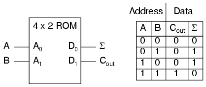
If this ROM has been written with the above data (representing a half-adder’s truth table), driving the A and B address inputs will cause the respective memory cells in the ROM chip to be enabled, thus outputting the corresponding data as the Σ (Sum) and C_out bits. Unlike the half-adder circuit built of gates or relays, this device can be set up to perform any logic function at all with two inputs and two outputs, not just the half-adder function. To change the logic function, all we would need to do is write a different table of data to another ROM chip. We could even use an EPROM chip which could be re-written at will, giving the ultimate flexibility in function.

It is vitally important to recognize the significance of this principle as applied to digital circuitry. Whereas the half-adder built from gates or relays processes the input bits to arrive at a specific output, the ROM simply remembers what the outputs should be for any given combination of inputs. This is not much different from the “times tables” memorized in grade school: rather than having to calculate the product of 5 times 6 (5 + 5 + 5 + 5 + 5 + 5 = 30), school-children are taught to remember that 5 x 6 = 30, and then expected to recall this product from memory as needed. Likewise, rather than the logic function depending on the functional arrangement of hard-wired gates or relays (hardware), it depends solely on the data written into the memory (software).

Such a simple application, with definite outputs for every input, is called a look-up table, because the memory device simply “looks up” what the output(s) should to be for any given combination of inputs states.

This application of a memory device to perform logical functions is significant for several reasons:

• Software is much easier to change than hardware.
• Software can be archived on various kinds of memory media (disk, tape), thus providing an easy way to document and manipulate the function in a “virtual” form; hardware can only be “archived” abstractly in the form of some kind of graphical drawing.
• Software can be copied from one memory device (such as the EPROM chip) to another, allowing the ability for one device to “learn” its function from another device.
• Software such as the logic function example can be designed to perform functions that would be extremely difficult to emulate with discrete logic gates (or relays!).

The usefulness of a look-up table becomes more and more evident with increasing complexity of function. Suppose we wanted to build a 4-bit adder circuit using a ROM. We’d require a ROM with 8 address lines (two 4-bit numbers to be added together), plus 4 data lines (for the signed output):



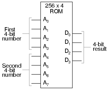
With 256 addressable memory locations in this ROM chip, we would have a fair amount of programming to do, telling it what binary output to generate for each and every combination of binary inputs. We would also run the risk of making a mistake in our programming and have it output an incorrect sum, if we weren’t careful. However, the flexibility of being able to configure this function (or any function) through software alone generally outweighs that costs.

Consider some of the advanced functions we could implement with the above “adder.” We know that when we add two sets of numbers in 2’s complement signed notation, we risk having the answer overflow. For instance, if we try to add 0111 (decimal 7) to 0110 (decimal 6) with only a 4-bit number field, the answer we’ll get is 1001 (decimal -7) instead of the correct value, 13 (7 + 6), which cannot be expressed using 4 signed bits. If we wanted to, we could avoid the strange answers given in overflow conditions by programming this look-up table circuit to output something else in conditions where we know overflow will occur (that is, in any case where the real sum would exceed +7 or -8). One alternative might be to program the ROM to output the quantity 0111 (the maximum positive value that can be represented with 4 signed bits), or any other value that we determined to be more appropriate for the application than the typical overflowed “error” value that a regular adder circuit would output. It’s all up to the programmer to decide what he or she wants this circuit to do, because we are no longer limited by the constraints of logic gate functions.

The possibilities don’t stop at customized logic functions, either. By adding more address lines to the 256 x 4 ROM chip, we can expand the look-up table to include multiple functions:



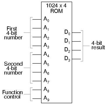
With two more address lines, the ROM chip will have 4 times as many addresses as before (1024 instead of 256). This ROM could be programmed so that when A8 and A9 were both low, the output data represented the sum of the two 4-bit binary numbers input on address lines A0 through A7, just as we had with the previous 256 x 4 ROM circuit. For the addresses A8=1 and A9=0, it could be programmed to output the difference (subtraction) between the first 4-bit binary number (A0 through A3) and the second binary number (A4 through A7). For the addresses A8=0 and A9=1, we could program the ROM to output the difference (subtraction) of the two numbers in reverse order (second - first rather than first - second), and finally, for the addresses A8=1 and A9=1, the ROM could be programmed to compare the two inputs and output an indication of equality or inequality. What we will have then is a device that can perform four different arithmetical operations on 4-bit binary numbers, all by “looking up” the answers programmed into it.

If we had used a ROM chip with more than two additional address lines, we could program it with a wider variety of functions to perform on the two 4-bit inputs. There are a number of operations peculiar to binary data (such as parity check or Exclusive-ORing of bits) that we might find useful to have programmed in such a look-up table.

Devices such as this, which can perform a variety of arithmetical tasks as dictated by a binary input code, are known as Arithmetic Logic Units (ALUs), and they comprise one of the essential components of computer technology. Although modern ALUs are more often constructed from very complex combinational logic (gate) circuits for reasons of speed, it should be comforting to know that the exact same functionality may be duplicated with a “dumb” ROM chip programmed with the appropriate look-up table(s). In fact, this exact approach was used by IBM engineers in 1959 with the development of the IBM 1401 and 1620 computers, which used look-up tables to perform addition, rather than binary adder circuitry. The machine was fondly known as the “CADET,” which stood for “Can’t Add, Doesn’t Even Try.”

A very common application for look-up table ROMs is in control systems where a custom mathematical function needs to be represented. Such an application is found in computer-controlled fuel injection systems for automobile engines, where the proper air/fuel mixture ratio for efficient and clean operation changes with several environmental and operational variables. Tests performed on engines in research laboratories determine what these ideal ratios are for varying conditions of engine load, ambient air temperature, and barometric air pressure. The variables are measured with sensor transducers, their analog outputs converted to digital signals with A/D circuitry, and those parallel digital signals used as address inputs to a high-capacity ROM chip programmed to output the optimum digital value for air/fuel ratio for any of these given conditions.

Sometimes, ROMs are used to provide one-dimensional look-up table functions, for “correcting” digitized signal values so that they more accurately represent their real-world significance. An example of such a device is a thermocouple transmitter, which measures the millivoltage signal generated by a junction of dissimilar metals and outputs a signal which is supposed to directly correspond to that junction temperature. Unfortunately, thermocouple junctions do not have perfectly linear temperature/voltage responses, and so the raw voltage signal is not perfectly proportional to temperature. By digitizing the voltage signal (A/D conversion) and sending that digital value to the address of a ROM programmed with the necessary correction values, the ROM’s programming could eliminate some of the nonlinearity of the thermocouple’s temperature-to-millivoltage relationship, so that the final output of the device would be more accurate. The popular instrumentation term for such a look-up table is a digital characterizer.



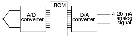
Another application for look-up tables is in special code translation. A 128 x 8 ROM, for instance, could be used to translate 7-bit ASCII code to 8-bit EBCDIC code:



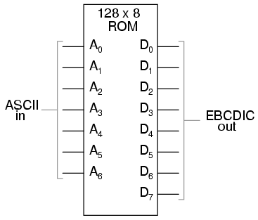
Again, all that is required is for the ROM chip to be properly programmed with the necessary data so that each valid ASCII input will produce a corresponding EBCDIC output code.




Finite-state Machine   

Feedback is a fascinating engineering principle. It can turn a rather simple device or process into something substantially more complex. We’ve seen the effects of feedback intentionally integrated into circuit designs with some rather astounding effects:

• Comparator + negative feedback—————-> controllable-gain amplifier
• Comparator + positive feedback—————-> comparator with hysteresis
• Combinational logic + positive feedback—> multivibrator

In the field of process instrumentation, feedback is used to transform a simple measurement system into something capable of control:

• Measurement system + negative feedback—-> closed-loop control system

Feedback, both positive and negative, has the tendency to add whole new dynamics to the operation of a device or system. Sometimes, these new dynamics find useful application, while other times they are merely interesting. With look-up tables programmed into memory devices, feedback from the data outputs back to the address inputs creates a whole new type of device: the Finite State Machine, or FSM:



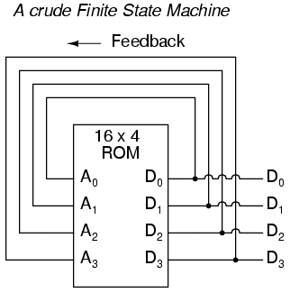
The above circuit illustrates the basic idea: the data stored at each address becomes the next storage location that the ROM gets addressed to. The result is a specific sequence of binary numbers (following the sequence programmed into the ROM) at the output, over time. To avoid signal timing problems, though, we need to connect the data outputs back to the address inputs through a 4-bit D-type flip-flop, so that the sequence takes place step by step to the beat of a controlled clock pulse:



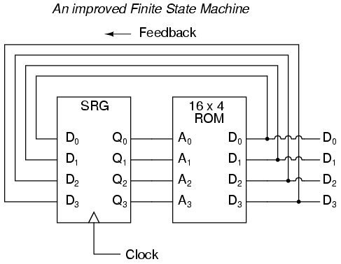
An analogy for the workings of such a device might be an array of post-office boxes, each one with an identifying number on the door (the address), and each one containing a piece of paper with the address of another P.O. box written on it (the data). A person, opening the first P.O. box, would find in it the address of the next P.O. box to open. By storing a particular pattern of addresses in the P.O. boxes, we can dictate the sequence in which each box gets opened, and therefore the sequence of which paper gets read.

Having 16 addressable memory locations in the ROM, this Finite State Machine would have 16 different stable “states” in which it could latch. In each of those states, the identity of the next state would be programmed in to the ROM, awaiting the signal of the next clock pulse to be fed back to the ROM as an address. One useful application of such an FSM would be to generate an arbitrary count sequence, such as Gray Code:

Address  -----> Data          Gray Code count sequence:
0000   -------> 0001                 0   0000
0001   -------> 0011                 1   0001
0010   -------> 0110                 2   0011
0011   -------> 0010                 3   0010
0100   -------> 1100                 4   0110
0101   -------> 0100                 5   0111
0110   -------> 0111                 6   0101
0111   -------> 0101                 7   0100
1000   -------> 0000                 8   1100
1001   -------> 1000                 9   1101
1010   -------> 1011                10   1111
1011   -------> 1001                11   1110
1100   -------> 1101                12   1010
1101   -------> 1111                13   1011
1110   -------> 1010                14   1001
1111   -------> 1110                15   1000

Try to follow the Gray Code count sequence as the FSM would do it: starting at 0000, follow the data stored at that address (0001) to the next address, and so on (0011), and so on (0010), and so on (0110), etc. The result, for the program table shown, is that the sequence of addressing jumps around from address to address in what looks like a haphazard fashion, but when you check each address that is accessed, you will find that it follows the correct order for 4-bit Gray code. When the FSM arrives at its last programmed state (address 1000), the data stored there is 0000, which starts the whole sequence over again at address 0000 in step with the next clock pulse.

We could expand on the capabilities of the above circuit by using a ROM with more address lines, and adding more programming data:



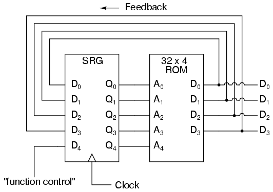
Now, just like the look-up table adder circuit that we turned into an Arithmetic Logic Unit (+, -, x, / functions) by utilizing more address lines as “function control” inputs, this FSM counter can be used to generate more than one count sequence, a different sequence programmed for the four feedback bits (A0 through A3) for each of the two function control line input combinations (A4 = 0 or 1).

Address  -----> Data            Address  -----> Data 
00000  -------> 0001            10000  -------> 0001 
00001  -------> 0010            10001  -------> 0011 
00010  -------> 0011            10010  -------> 0110 
00011  -------> 0100            10011  -------> 0010 
00100  -------> 0101            10100  -------> 1100 
00101  -------> 0110            10101  -------> 0100 
00110  -------> 0111            10110  -------> 0111 
00111  -------> 1000            10111  -------> 0101 
01000  -------> 1001            11000  -------> 0000 
01001  -------> 1010            11001  -------> 1000 
01010  -------> 1011            11010  -------> 1011 
01011  -------> 1100            11011  -------> 1001 
01100  -------> 1101            11100  -------> 1101 
01101  -------> 1110            11101  -------> 1111 
01110  -------> 1111            11110  -------> 1010 
01111  -------> 0000            11111  -------> 1110

If A4 is 0, the FSM counts in binary; if A4 is 1, the FSM counts in Gray Code. In either case, the counting sequence is arbitrary: determined by the whim of the programmer. For that matter, the counting sequence doesn’t even have to have 16 steps, as the programmer may decide to have the sequence recycle to 0000 at any one of the steps at all. It is a completely flexible counting device, the behavior strictly determined by the software (programming) in the ROM.

We can expand on the capabilities of the FSM even more by utilizing a ROM chip with additional address input and data output lines. Take the following circuit, for example:





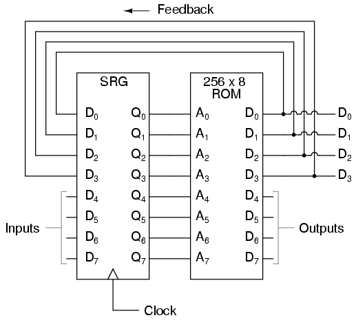
Here, the D0 through D3 data outputs are used exclusively for feedback to the A0 through A3 address lines. Date output lines D4 through D7 can be programmed to output something other than the FSM’s “state” value. Being that four data output bits are being fed back to four address bits, this is still a 16-state device. However, having the output data come from other data output lines gives the programmer more freedom to configure functions than before. In other words, this device can do far more than just count! The programmed output of this FSM is dependent not only upon the state of the feedback address lines (A0 through A3), but also the states of the input lines (A4 through A7). The D-type flip/flop’s clock signal input does not have to come from a pulse generator, either. To make things more interesting, the flip/flop could be wired up to clock on some external event, so that the FSM goes to the next state only when an input signal tells it to.

Now we have a device that better fulfills the meaning of the word “programmable.” The data written to the ROM is a program in the truest sense: the outputs follow a pre-established order based on the inputs to the device and which “step” the device is on in its sequence. This is very close to the operating design of the Turing Machine, a theoretical computing device invented by Alan Turing, mathematically proven to be able to solve any known arithmetic problem, given enough memory capacity


Microprocessors 

Early computer science pioneers such as Alan Turing and John Von Neumann postulated that for a computing device to be really useful, it not only had to be able to generate specific outputs as dictated by programmed instructions, but it also had to be able to write data to memory, and be able to act on that data later. Both the program steps and the processed data were to reside in a common memory “pool,” thus giving way to the label of the stored-program computer. Turing’s theoretical machine utilized a sequential-access tape, which would store data for a control circuit to read, the control circuit re-writing data to the tape and/or moving the tape to a new position to read more data. Modern computers use random-access memory devices instead of sequential-access tapes to accomplish essentially the same thing, except with greater capability.

A helpful illustration is that of early automatic machine tool control technology. Called open-loop, or sometimes just NC (numerical control), these control systems would direct the motion of a machine tool such as a lathe or a mill by following instructions programmed as holes in paper tape. The tape would be run one direction through a “read” mechanism, and the machine would blindly follow the instructions on the tape without regard to any other conditions. While these devices eliminated the burden of having to have a human machinist direct every motion of the machine tool, it was limited in usefulness. Because the machine was blind to the real world, only following the instructions written on the tape, it could not compensate for changing conditions such as expansion of the metal or wear of the mechanisms. Also, the tape programmer had to be acutely aware of the sequence of previous instructions in the machine’s program to avoid troublesome circumstances (such as telling the machine tool to move the drill bit laterally while it is still inserted into a hole in the work), since the device had no memory other than the tape itself, which was read-only. Upgrading from a simple tape reader to a Finite State control design gave the device a sort of memory that could be used to keep track of what it had already done (through feedback of some of the data bits to the address bits), so at least the programmer could decide to have the circuit remember “states” that the machine tool could be in (such as “coolant on,” or tool position). However, there was still room for improvement.

The ultimate approach is to have the program give instructions which would include the writing of new data to a read/write (RAM) memory, which the program could easily recall and process. This way, the control system could record what it had done, and any sensor-detectable process changes, much in the same way that a human machinist might jot down notes or measurements on a scratch-pad for future reference in his or her work. This is what is referred to as CNC, or Closed-loop Numerical Control.

Engineers and computer scientists looked forward to the possibility of building digital devices that could modify their own programming, much the same as the human brain adapts the strength of inter-neural connections depending on environmental experiences (that is why memory retention improves with repeated study, and behavior is modified through consequential feedback). Only if the computer’s program were stored in the same writable memory “pool” as the data would this be practical. It is interesting to note that the notion of a self-modifying program is still considered to be on the cutting edge of computer science. Most computer programming relies on rather fixed sequences of instructions, with a separate field of data being the only information that gets altered.

To facilitate the stored-program approach, we require a device that is much more complex than the simple FSM, although many of the same principles apply. First, we need read/write memory that can be easily accessed: this is easy enough to do. Static or dynamic RAM chips do the job well, and are inexpensive. Secondly, we need some form of logic to process the data stored in memory. Because standard and Boolean arithmetic functions are so useful, we can use an Arithmetic Logic Unit (ALU) such as the look-up table ROM example explored earlier. Finally, we need a device that controls how and where data flows between the memory, the ALU, and the outside world. This so-called Control Unit is the most mysterious piece of the puzzle yet, being comprised of tri-state buffers (to direct data to and from buses) and decoding logic which interprets certain binary codes as instructions to carry out. Sample instructions might be something like: “add the number stored at memory address 0010 with the number stored at memory address 1101,” or, “determine the parity of the data in memory address 0111.” The choice of which binary codes represent which instructions for the Control Unit to decode is largely arbitrary, just as the choice of which binary codes to use in representing the letters of the alphabet in the ASCII standard was largely arbitrary. ASCII, however, is now an internationally recognized standard, whereas control unit instruction codes are almost always manufacturer-specific.

Putting these components together (read/write memory, ALU, and control unit) results in a digital device that is typically called a processor. If minimal memory is used, and all the necessary components are contained on a single integrated circuit, it is called a microprocessor. When combined with the necessary bus-control support circuitry, it is known as a Central Processing Unit, or CPU.

CPU operation is summed up in the so-called fetch/execute cycle. Fetch means to read an instruction from memory for the Control Unit to decode. A small binary counter in the CPU (known as the program counter or instruction pointer) holds the address value where the next instruction is stored in main memory. The Control Unit sends this binary address value to the main memory’s address lines, and the memory’s data output is read by the Control Unit to send to another holding register. If the fetched instruction requires reading more data from memory (for example, in adding two numbers together, we have to read both the numbers that are to be added from main memory or from some other source), the Control Unit appropriately addresses the location of the requested data and directs the data output to ALU registers. Next, the Control Unit would execute the instruction by signaling the ALU to do whatever was requested with the two numbers, and direct the result to another register called the accumulator. The instruction has now been “fetched” and “executed,” so the Control Unit now increments the program counter to step the next instruction, and the cycle repeats itself.

 Microprocessor (CPU)

--------------------------------------
|       ** Program counter **        |
|  (increments address value sent to |
|  external memory chip(s) to fetch  |==========> Address bus
|  the next instruction)             |          (to RAM memory)
--------------------------------------
|        ** Control Unit **          |<=========> Control Bus
|  (decodes instructions read from   | (to all devices sharing
|  program in memory, enables flow   | address and/or data busses;
|  of data to and from ALU, internal | arbitrates all bus communi- 
|  registers, and external devices)  | cations)
-------------------------------------- 
| ** Arithmetic Logic Unit (ALU) **  |
|    (performs all mathematical      |
|     calculations and Boolean       |
|     functions)                     |
--------------------------------------
|          ** Registers **           |
|    (small read/write memories for  |<=========> Data Bus
|     holding instruction codes,     | (from RAM memory and other
|     error codes, ALU data, etc;    |  external devices)
|     includes the "accumulator")    |
--------------------------------------

As one might guess, carrying out even simple instructions is a tedious process. Several steps are necessary for the Control Unit to complete the simplest of mathematical procedures. This is especially true for arithmetic procedures such as exponents, which involve repeated executions (“iterations”) of simpler functions. Just imagine the sheer quantity of steps necessary within the CPU to update the bits of information for the graphic display on a flight simulator game! The only thing which makes such a tedious process practical is the fact that microprocessor circuits are able to repeat the fetch/execute cycle with great speed.

In some microprocessor designs, there are minimal programs stored within a special ROM memory internal to the device (called microcode) which handle all the sub-steps necessary to carry out more complex math operations. This way, only a single instruction has to be read from the program RAM to do the task, and the programmer doesn’t have to deal with trying to tell the microprocessor how to do every minute step. In essence, its a processor inside of a processor; a program running inside of a program.




Microprocessor Programming 

The “vocabulary” of instructions which any particular microprocessor chip possesses is specific to that model of chip. An Intel 80386, for example, uses a completely different set of binary codes than a Motorola 68020, for designating equivalent functions. Unfortunately, there are no standards in place for microprocessor instructions. This makes programming at the very lowest level very confusing and specialized.

When a human programmer develops a set of instructions to directly tell a microprocessor how to do something (like automatically control the fuel injection rate to an engine), they’re programming in the CPU’s own “language.” This language, which consists of the very same binary codes which the Control Unit inside the CPU chip decodes to perform tasks, is often referred to as machine language. While machine language software can be “worded” in binary notation, it is often written in hexadecimal form, because it is easier for human beings to work with. For example, I’ll present just a few of the common instruction codes for the Intel 8080 micro-processor chip:

Hexadecimal    Binary              Instruction description
-----------   --------   -----------------------------------------
|   7B        01111011   Move contents of register A to register E
|
|   87        10000111   Add contents of register A to register D
|
|   1C        00011100   Increment the contents of register E by 1
|
|   D3        11010011   Output byte of data to data bus

Even with hexadecimal notation, these instructions can be easily confused and forgotten. For this purpose, another aid for programmers exists called assembly language. With assembly language, two to four letter mnemonic words are used in place of the actual hex or binary code for describing program steps. For example, the instruction 7B for the Intel 8080 would be “MOV A,E” in assembly language. The mnemonics, of course, are useless to the microprocessor, which can only understand binary codes, but it is an expedient way for programmers to manage the writing of their programs on paper or text editor (word processor). There are even programs written for computers called assemblers which understand these mnemonics, translating them to the appropriate binary codes for a specified target microprocessor, so that the programmer can write a program in the computer’s native language without ever having to deal with strange hex or tedious binary code notation.

Once a program is developed by a person, it must be written into memory before a microprocessor can execute it. If the program is to be stored in ROM (which some are), this can be done with a special machine called a ROM programmer, or (if you’re masochistic), by plugging the ROM chip into a breadboard, powering it up with the appropriate voltages, and writing data by making the right wire connections to the address and data lines, one at a time, for each instruction. If the program is to be stored in volatile memory, such as the operating computer’s RAM memory, there may be a way to type it in by hand through that computer’s keyboard (some computers have a mini-program stored in ROM which tells the microprocessor how to accept keystrokes from a keyboard and store them as commands in RAM), even if it is too dumb to do anything else. Many “hobby” computer kits work like this. If the computer to be programmed is a fully-functional personal computer with an operating system, disk drives, and the whole works, you can simply command the assembler to store your finished program onto a disk for later retrieval. To “run” your program, you would simply type your program’s filename at the prompt, press the Enter key, and the microprocessor’s Program Counter register would be set to point to the location (“address”) on the disk where the first instruction is stored, and your program would run from there.

Although programming in machine language or assembly language makes for fast and highly efficient programs, it takes a lot of time and skill to do so for anything but the simplest tasks, because each machine language instruction is so crude. The answer to this is to develop ways for programmers to write in “high level” languages, which can more efficiently express human thought. Instead of typing in dozens of cryptic assembly language codes, a programmer writing in a high-level language would be able to write something like this . . .

Print "Hello, world!" 

. . . and expect the computer to print “Hello, world!” with no further instruction on how to do so. This is a great idea, but how does a microprocessor understand such “human” thinking when its vocabulary is so limited?

The answer comes in two different forms: interpretation, or compilation. Just like two people speaking different languages, there has to be some way to transcend the language barrier in order for them to converse. A translator is needed to translate each person’s words to the other person’s language, one way at a time. For the microprocessor, this means another program, written by another programmer in machine language, which recognizes the ASCII character patterns of high-level commands such as Print (P-r-i-n-t) and can translate them into the necessary bite-size steps that the microprocessor can directly understand. If this translation is done during program execution, just like a translator intervening between two people in a live conversation, it is called “interpretation.” On the other hand, if the entire program is translated to machine language in one fell swoop, like a translator recording a monologue on paper and then translating all the words at one sitting into a written document in the other language, the process is called “compilation.”

Interpretation is simple, but makes for a slow-running program because the microprocessor has to continually translate the program between steps, and that takes time. Compilation takes time initially to translate the whole program into machine code, but the resulting machine code needs no translation after that and runs faster as a consequence. Programming languages such as BASIC and FORTH are interpreted. Languages such as C, C++, FORTRAN, and PASCAL are compiled. Compiled languages are generally considered to be the languages of choice for professional programmers, because of the efficiency of the final product.

Naturally, because machine language vocabularies vary widely from microprocessor to microprocessor, and since high-level languages are designed to be as universal as possible, the interpreting and compiling programs necessary for language translation must be microprocessor-specific. Development of these interpreters and compilers is a most impressive feat: the people who make these programs most definitely earn their keep, especially when you consider the work they must do to keep their software product current with the rapidly-changing microprocessor models appearing on the market!

To mitigate this difficulty, the trend-setting manufacturers of microprocessor chips (most notably, Intel and Motorola) try to design their new products to be backwardly compatible with their older products. For example, the entire instruction set for the Intel 80386 chip is contained within the latest Pentium IV chips, although the Pentium chips have additional instructions that the 80386 chips lack. What this means is that machine-language programs (compilers, too) written for 80386 computers will run on the latest and greatest Intel Pentium IV CPU, but machine-language programs written specifically to take advantage of the Pentium’s larger instruction set will not run on an 80386, because the older CPU simply doesn’t have some of those instructions in its vocabulary: the Control Unit inside the 80386 cannot decode them.

Building on this theme, most compilers have settings that allow the programmer to select which CPU type he or she wants to compile machine-language code for. If they select the 80386 setting, the compiler will perform the translation using only instructions known to the 80386 chip; if they select the Pentium setting, the compiler is free to make use of all instructions known to Pentiums. This is analogous to telling a translator what minimum reading level their audience will be: a document translated for a child will be understandable to an adult, but a document translated for an adult may very well be gibberish to a child


                                        X  .  IIIII  Programmable logic controller 

A programmable logic controller (PLC), or programmable controller is an industrial digital computer which has been ruggedised and adapted for the control of manufacturing processes, such as assembly lines, or robotic devices, or any activity that requires high reliability control and ease of programming and process fault diagnosis.
They were first developed in the automobile industry to provide flexible, ruggedised and easily programmable controllers to replace hard-wired relays and timers. Since then they have been widely adopted as high-reliability automation controllers suitable for harsh environments. A PLC is an example of a "hard" real-time system since output results must be produced in response to input conditions within a limited time, otherwise unintended operation will result.

PLCs can range from small "building brick" devices with tens of inputs and outputs (I/O), in a housing integral with the processor, to large rack-mounted modular devices with a count of thousands of I/O, and which are often networked to other PLC and SCADA systems.
They can be designed for multiple arrangements of digital and analog I/O, extended temperature ranges, immunity to electrical noise, and resistance to vibration and impact. Programs to control machine operation are typically stored in battery-backed-up or non-volatile memory.
It was from the automotive industry in the USA that the PLC was born. Before the PLC, control, sequencing, and safety interlock logic for manufacturing automobiles was mainly composed of relays, cam timers, drum sequencers, and dedicated closed-loop controllers. Since these could number in the hundreds or even thousands, the process for updating such facilities for the yearly model change-over was very time consuming and expensive, as electricians needed to individually rewire the relays to change their operational characteristics.
When digital computers became available, being general-purpose programmable devices, they were soon applied to control sequential and combinatorial logic in industrial processes. However these early computers required specialist programmers and stringent operating environmental control for temperature, cleanliness, and power quality. To meet these challenges the PLC was developed with several key attributes. It would tolerate the shop-floor environment, it would support discrete (bit-form) input and output in an easily extensible manner, it would not require years of training to use, and it would permit its operation to be monitored. Since many industrial processes have timescales easily addressed by millisecond response times, modern (fast, small, reliable) electronics greatly facilitate building reliable controllers, and performance could be traded off for reliability.

Invention and early development

In 1968 GM Hydra-Matic (the automatic transmission division of General Motors) issued a request for proposals for an electronic replacement for hard-wired relay systems based on a white paper written by engineer Edward R. Clark. The winning proposal came from Bedford Associates of Bedford, Massachusetts. The first PLC, designated the 084 because it was Bedford Associates' eighty-fourth project, was the result.^[2] Bedford Associates started a new company dedicated to developing, manufacturing, selling, and servicing this new product: Modicon, which stood for MOdular DIgital CONtroller. One of the people who worked on that project was Dick Morley, who is considered to be the "father" of the PLC.^[3] The Modicon brand was sold in 1977 to Gould Electronics, later acquired by German Company AEG, and then by French Schneider Electric, the current owner.
One of the very first 084 models built is now on display at Schneider Electric's facility in North Andover, Massachusetts. It was presented to Modicon by GM, when the unit was retired after nearly twenty years of uninterrupted service. Modicon used the 84 moniker at the end of its product range until the 984 made its appearance.
The automotive industry is still one of the largest users of PLCs.
Early PLCs were designed to replace relay logic systems. These PLCs were programmed in "ladder logic", which strongly resembles a schematic diagram of relay logic. This program notation was chosen to reduce training demands for the existing technicians. Other early PLCs used a form of instruction list programming, based on a stack-based logic solver.
Modern PLCs can be programmed in a variety of ways, from the relay-derived ladder logic to programming languages such as specially adapted dialects of BASIC and C. Another method is state logic, a very high-level programming language designed to program PLCs based on state transition diagrams. The majority of PLC systems today adhere to the IEC 61131/3 control systems programming standard that defines 5 languages: Ladder Diagram (LD), Structured Text (ST), Function Block Diagram (FBD), Instruction List (IL) and Sequential Flow Chart (SFC).
Many early PLCs did not have accompanying programming terminals that were capable of graphical representation of the logic, and so the logic was instead represented as a series of logic expressions in some version of Boolean format, similar to Boolean algebra. As programming terminals evolved, it became more common for ladder logic to be used, for the aforementioned reasons and because it was a familiar format used for electromechanical control panels. Newer formats such as state logic and Function Block (which is similar to the way logic is depicted when using digital integrated logic circuits) exist, but they are still not as popular as ladder logic. A primary reason for this is that PLCs solve the logic in a predictable and repeating sequence, and ladder logic allows the programmer (the person writing the logic) to see any issues with the timing of the logic sequence more easily than would be possible in other formats.

Programming

Early PLCs, up to the mid-1990s, were programmed using proprietary programming panels or special-purpose programming terminals, which often had dedicated function keys representing the various logical elements of PLC programs.^[2] Some proprietary programming terminals displayed the elements of PLC programs as graphic symbols, but plain ASCII character representations of contacts, coils, and wires were common. Programs were stored on cassette tape cartridges. Facilities for printing and documentation were minimal due to lack of memory capacity. The oldest PLCs used non-volatile magnetic core memory.
More recently, PLCs are programmed using application software on personal computers, which now represent the logic in graphic form instead of character symbols. The computer is connected to the PLC through USB, Ethernet, RS-232, RS-485, or RS-422 cabling. The programming software allows entry and editing of the ladder-style logic. In some software packages, it is also possible to view and edit the program in function block diagrams, sequence flow charts and structured text. Generally the software provides functions for debugging and troubleshooting the PLC software, for example, by highlighting portions of the logic to show current status during operation or via simulation. The software will upload and download the PLC program, for backup and restoration purposes. In some models of programmable controller, the program is transferred from a personal computer to the PLC through a programming board which writes the program into a removable chip such as an EPROM.

Basics of programming

There are two types of contacts in PLC's and they are normally open and normally closed switches. A normally open contact means the contact is on when pressed/closed, and a normally closed contact is on when open/not pressed. Contacts represent the states of real world inputs like sensors, switches, if the part is present, empty, full, etc. PLC's also consist of coils, which are outputs like motors, pumps, lights, timers, etc. The PLC examines inputs and turns coils on or off whenever it is needed. They can also be used as inputs to other rungs in the ladder diagram.

Functionality

The functionality of the PLC has evolved over the years to include sequential relay control, motion control, process control, distributed control systems, and networking. The data handling, storage, processing power, and communication capabilities of some modern PLCs are approximately equivalent to desktop computers. PLC-like programming combined with remote I/O hardware, allow a general-purpose desktop computer to overlap some PLCs in certain applications. Desktop computer controllers have not been generally accepted in heavy industry because the desktop computers run on less stable operating systems than do PLCs, and because the desktop computer hardware is typically not designed to the same levels of tolerance to temperature, humidity, vibration, and longevity as the processors used in PLCs. Operating systems such as Windows do not lend themselves to deterministic logic execution, with the result that the controller may not always respond to changes of input status with the consistency in timing expected from PLCs. Desktop logic applications find use in less critical situations, such as laboratory automation and use in small facilities where the application is less demanding and critical, because they are generally much less expensive than PLCs.

Basic and complex functions

The most basic function of a Programmable logic controller (PLC) is to receive inputs from status components, which can be from sensors or switches. Some of the basic components of a PLC are input modules, a central processing unit, output modules, and a programming device. When an input is activated, some output will also be activated by whatever the machine is told to do. Some examples of this are setting a timer to 10ms, activating the timer and once 10ms have passed a siren goes off. Some advantages to using a PLC over other programming devices are the user doesn't have to rewire anything, the PLC has very little downtime in between running different programs, the user can program off-line, and PLC's aren't time constrained. If the user tells the PLC to perform an output in 10ms, it will perform the output in 10ms unlike other programs like LabView which can have a delay in activation. ^[5]

Timers and counters

The main function of a timer is to keep an output on for a specific length of time. A good example of this is a garage light, where you want power to be cut off after 2 minutes so as to give someone time to go into the house. The three different types of timers that are commonly used are a Delay-OFF, a Delay-ON, and a Delay-ON-Retentive. A Delay-OFF timer activates immediately when turned on, counts down from a programmed time before cutting off, and is cleared when the enabling input is off. A Delay-ON timer is activated by input and starts accumulating time, counts up to a programmed time before cutting off, and is cleared when the enabling input is turned off. A Delay-ON-Retentive timer is activated by input and starts accumulating time, retains the accumulated value even if the (ladder-logic) rung goes false, and can be resets only by a RESET contact.
Counters are primarily used for counting items such as cans going into a box on an assembly line. This is important because once something is filled to its max the item needs to be moved on so something else can be filled. Many companies use counters in PLC's to count boxes, count how many feet of something is covered, or to count how many pallets are on a truck. There are three types of counters, Up counters, Down counters, and Up/Down counters. Up counters count up to the preset value, turn on the CTU (CounT Up output) when the preset value is reached, and are cleared upon receiving a reset. Down counters count down from a preset value, turns on the CTD (CounT Down output) when 0 is reached, and are cleared upon reset. Up/Down counters count up on CU, count down on CD, turn on CTUD (CounT Up/Down output) when the preset value is reached, and cleared on reset. ^[6]

Programmable logic relay (PLR)

In more recent years, small products called PLRs (programmable logic relays), and also by similar names, have become more common and accepted. These are much like PLCs, and are used in light industry where only a few points of I/O (i.e. a few signals coming in from the real world and a few going out) are needed, and low cost is desired. These small devices are typically made in a common physical size and shape by several manufacturers, and branded by the makers of larger PLCs to fill out their low end product range. Popular names include PICO Controller, NANO PLC, and other names implying very small controllers. Most of these have 8 to 12 discrete inputs, 4 to 8 discrete outputs, and up to 2 analog inputs. Size is usually about 4" wide, 3" high, and 3" deep. Most such devices include a tiny postage-stamp-sized LCD screen for viewing simplified ladder logic (only a very small portion of the program being visible at a given time) and status of I/O points, and typically these screens are accompanied by a 4-way rocker push-button plus four more separate push-buttons, similar to the key buttons on a VCR remote control, and used to navigate and edit the logic. One company, Preferred Utilities, in Danbury, CT, has a slightly larger model with a 5-inch screen. Most have a small plug for connecting via RS-232 or RS-485 to a personal computer so that programmers can use simple Windows applications for programming instead of being forced to use the tiny LCD and push-button set for this purpose. Unlike regular PLCs that are usually modular and greatly expandable, the PLRs are usually not modular or expandable, but their price can be two orders of magnitude less than a PLC, and they still offer robust design and deterministic execution of the logics.

PLC topics

Features

Control panel with PLC (grey elements in the center). The unit consists of separate elements, from left to right; power supply, controller, relay units for in- and output

Control panel with an Allen-Bradley PLC user interface for thermal oxidizer regulation.

The main difference from most other computing devices is that PLCs are intended-for and therefore tolerant-of more severe conditions (such as dust, moisture, heat, cold), while offering extensive input/output (I/O) to connect the PLC to sensors and actuators. PLC input can include simple digital elements such as limit switches, analog variables from process sensors (such as temperature and pressure), and more complex data such as that from positioning or machine vision systems.^[7] PLC output can include elements such as indicator lamps, sirens, electric motors, pneumatic or hydraulic cylinders, magnetic relays, solenoids, or analog outputs. The input/output arrangements may be built into a simple PLC, or the PLC may have external I/O modules attached to a computer network that plugs into the PLC.

Scan time

A PLC program generally loops i.e. executes repeatedly, as long as the controlled system is running. At the start of each execution loop, the status of all physical inputs are copied to an area of memory, sometimes called the "I/O Image Table", which is accessible to the processor. The program then runs from its first instruction rung down to the last rung. It takes some time for the processor of the PLC to evaluate all the rungs and update the I/O image table with the status of outputs.^[8] Scan times of a few milliseconds may be encountered for small programs and fast processors, but for older processors and very large programs much longer scan times (on the order of 100 ms) may be encountered. Excessively long scan times may mean the response of the PLC to changing inputs or process conditions is too slow to be useful.
As PLCs became more advanced, methods were developed to change the sequence of ladder execution, and subroutines were implemented.^[9] This simplified programming could be used to save scan time for high-speed processes; for example, parts of the program used only for setting up the machine could be segregated from those parts required to operate at higher speed.
Special-purpose I/O modules may be used where the scan time of the PLC is too long to allow predictable performance. Precision timing modules, or counter modules for use with shaft encoders, are used where the scan time would be too long to reliably count pulses or detect the sense of rotation of an encoder. This allows even a relatively slow PLC can still interpret the counted values to control a machine, as the accumulation of pulses is done by a dedicated module that is unaffected by the speed of program execution.

Process of a scan cycle

There are 5 main steps in a scan cycle:

1. Reading inputs
2. Executing the program
3. Processing communication requests
4. Executing CPU diagnostics
5. Writing outputs

To read the inputs, the user writes values to reserved bytes in image table for input values. When executing the program, the ladder is read from left to right, and top to bottom. When processing communication requests, the user processes any message received from the communications port. To execute the CPU Self-Diagnostic test, check the firmware, check the program, and check the status of the modules.

System scale

A small PLC will have a fixed number of connections built in for inputs and outputs. Typically, expansions are available if the base model has insufficient I/O.
Modular PLCs have a chassis (also called a rack) into which are placed modules with different functions. The processor and selection of I/O modules are customized for the particular application. Several racks can be administered by a single processor, and may have thousands of inputs and outputs. Either a special high speed serial I/O link or comparable communication method is used so that racks can be distributed away from the processor, reducing the wiring costs for large plants. Options are also available to mount I/O points directly to the machine and utilize quick disconnecting cables to sensors and valves, saving time for wiring and replacing components.

User interface

 

PLCs may need to interact with people for the purpose of configuration, alarm reporting, or everyday control. A human-machine interface (HMI) is employed for this purpose. HMIs are also referred to as man-machine interfaces (MMIs) and graphical user interfaces (GUIs). A simple system may use buttons and lights to interact with the user. Text displays are available as well as graphical touch screens. More complex systems use programming and monitoring software installed on a computer, with the PLC connected via a communication interface.

Communications

PLCs have built-in communications ports, usually 9-pin RS-232, RS-422, RS-485, Ethernet. Various protocols are usually included. Many of these protocols are vendor specific.
Most modern PLCs can communicate over a network to some other system, such as a computer running a SCADA (Supervisory Control And Data Acquisition) system or web browser.
PLCs used in larger I/O systems may have peer-to-peer (P2P) communication between processors. This allows separate parts of a complex process to have individual control while allowing the subsystems to co-ordinate over the communication link. These communication links are also often used for HMI devices such as keypads or PC-type workstations.
Formerly, some manufacturers offered dedicated communication modules as an add-on function where the processor had no network connection built-in.

Programming

PLC programs are typically written in a special application on a personal computer, then downloaded by a direct-connection cable or over a network to the PLC. The program is stored in the PLC either in battery-backed-up RAM or some other non- volatile flash memory. Often, a single PLC can be programmed to replace thousands of relays.^[11]
Under the IEC 61131-3 standard, PLCs can be programmed using standards-based programming languages. The most commonly used programming language is Ladder diagram (LD) also known as Ladder logic. It uses Contact-Coil logic to make programs like an electrical control diagram. A graphical programming notation called Sequential Function Charts is available on certain programmable controllers. A model which emulated electromechanical control panel devices (such as the contact and coils of relays) which PLCs replaced. This model remains common today.
IEC 61131-3 currently defines five programming languages for programmable control systems: function block diagram (FBD), ladder diagram (LD), structured text (ST; similar to the Pascal programming language), instruction list (IL; similar to assembly language), and sequential function chart (SFC).^[12] These techniques emphasize logical organization of operations.^[11]
While the fundamental concepts of PLC programming are common to all manufacturers, differences in I/O addressing, memory organization, and instruction sets mean that PLC programs are never perfectly interchangeable between different makers. Even within the same product line of a single manufacturer, different models may not be directly compatible.

Control example shown in ladder diagram

This is a programming example in ladder diagram which shows the control system. A ladder diagram is a method of drawing control circuits which pre-dates PLCs. The ladder diagram resembles the schematic diagram of a system built with electromechanical relays.
As an example, say a facility needs to store water in a tank. The water is drawn from the tank by another system, as needed, and our example system must manage the water level in the tank by controlling the valve that refills the tank. . Shown are:

• Two inputs (from the low and high level switches) represented by contacts of the float switches
• An output to the fill valve, labelled as the fill valve which it controls
• An "internal" contact, representing the output signal to the fill valve which is created in the program.
• A logical control scheme created by the interconnection of these items in software

In ladder diagram, the contact symbols represent the state of bits in processor memory, which corresponds to the state of physical inputs to the system. If a discrete input is energized, the memory bit is a 1, and a "normally open" contact controlled by that bit will pass a logic "true" signal on to the next element of the ladder. Therefore, the contacts in the PLC program that "read" or look at the physical switch contacts in this case must be "opposite" or open in order to return a TRUE for the closed physical switches. Internal status bits, corresponding to the state of discrete outputs, are also available to the program.
In the example, the physical state of the float switch contacts must be considered when choosing "normally open" or "normally closed" symbols in the ladder diagram. The PLC has two discrete inputs from float switches (Low Level and High Level). Both float switches (normally closed) open their contacts when the water level in the tank is above the physical location of the switch.
When the water level is below both switches, the float switch physical contacts are both closed, and a true (logic 1) value is passed to the Fill Valve output. Water begins to fill the tank. The internal "Fill Valve" contact latches the circuit so that even when the "Low Level" contact opens (as the water passes the lower switch), the fill valve remains on. Since the High Level is also normally closed, water continues to flow as the water level remains between the two switch levels. Once the water level rises enough so that the "High Level" switch is off (opened), the PLC will shut the inlet to stop the water from overflowing; this is an example of seal-in (latching) logic. The output is sealed in until a high level condition breaks the circuit. After that the fill valve remains off until the level drops so low that the Low Level switch is activated, and the process repeats again.

| (N.C. physical   (N.C. physical                             |
|   Switch)          Switch)                                  |
|   Low Level       High Level                Fill Valve      |
|------[ ]------|------[ ]----------------------(OUT)---------|
|               |                                             |
|               |                                             |
|               |                                             |
|   Fill Valve  |                                             |
|------[ ]------|                                             |
|                                                             |
|                                                             |

A complete program may contain thousands of rungs, evaluated in sequence. Typically the PLC processor will alternately scan all its inputs and update outputs, then evaluate the ladder logic; input changes during a program scan will not be effective until the next I/O update. A complete program scan may take only a few milliseconds, much faster than changes in the controlled process.
Programmable controllers vary in their capabilities for a "rung" of a ladder diagram. Some only allow a single output bit. There are typically limits to the number of series contacts in line, and the number of branches that can be used. Each element of the rung is evaluated sequentially. If elements change their state during evaluation of a rung, hard-to-diagnose faults can be generated, although sometimes (as above) the technique is useful. Some implementations forced evaluation from left-to-right as displayed and did not allow reverse flow of a logic signal (in multi-branched rungs) to affect the output.

Security

Prior to the discovery of the Stuxnet computer worm in June 2010, security of PLCs received little attention. PLCs generally contain a real-time operating system such as OS-9 or VxWorks, and exploits for these systems exist much as they do for desktop computer operating systems such as Microsoft Windows. PLCs can also be attacked by gaining control of a computer they communicate with.^[13]

Simulation

PLCLogix PLC Simulation Software

In order to properly understand the operation of a PLC, it is necessary to spend considerable time programming, testing, and debugging PLC programs. PLC systems are inherently expensive, and down-time is often very costly. In addition, if a PLC is programmed incorrectly it can result in lost productivity and dangerous conditions. PLC simulation software such as PLCLogix can save time in the design of automated control applications and can also increase the level of safety associated with equipment since various "what if" scenarios can be tried and tested before the system is activated.

Redundancy

Some special processes need to work permanently with minimum unwanted down time. Therefore, it is necessary to design a system which is fault-tolerant and capable of handling the process with faulty modules. In such cases to increase the system availability in the event of hardware component failure, redundant CPU or I/O modules with the same functionality can be added to hardware configuration for preventing total or partial process shutdown due to hardware failure.

PLC compared with other control systems

Allen-Bradley PLC installed in a control panel

Control center with an Allen-Bradley PLC for a RTO.

PLCs are well adapted to a range of automation tasks. These are typically industrial processes in manufacturing where the cost of developing and maintaining the automation system is high relative to the total cost of the automation, and where changes to the system would be expected during its operational life. PLCs contain input and output devices compatible with industrial pilot devices and controls; little electrical design is required, and the design problem centers on expressing the desired sequence of operations. PLC applications are typically highly customized systems, so the cost of a packaged PLC is low compared to the cost of a specific custom-built controller design. On the other hand, in the case of mass-produced goods, customized control systems are economical. This is due to the lower cost of the components, which can be optimally chosen instead of a "generic" solution, and where the non-recurring engineering charges are spread over thousands or millions of units.
For high volume or very simple fixed automation tasks, different techniques are used. For example, a cheap consumer dishwasher would be controlled by an electromechanical cam timer costing only a few dollars in production quantities.
A microcontroller-based design would be appropriate where hundreds or thousands of units will be produced and so the development cost (design of power supplies, input/output hardware, and necessary testing and certification) can be spread over many sales, and where the end-user would not need to alter the control. Automotive applications are an example; millions of units are built each year, and very few end-users alter the programming of these controllers. However, some specialty vehicles such as transit buses economically use PLCs instead of custom-designed controls, because the volumes are low and the development cost would be uneconomical.^[15]
Very complex process control, such as used in the chemical industry, may require algorithms and performance beyond the capability of even high-performance PLCs. Very high-speed or precision controls may also require customized solutions; for example, aircraft flight controls. Single-board computers using semi-customized or fully proprietary hardware may be chosen for very demanding control applications where the high development and maintenance cost can be supported. "Soft PLCs" running on desktop-type computers can interface with industrial I/O hardware while executing programs within a version of commercial operating systems adapted for process control needs.^[15]
Programmable controllers are widely used in motion, positioning, and/or torque control. Some manufacturers produce motion control units to be integrated with PLC so that G-code (involving a CNC machine) can be used to instruct machine movements.^{[16][citation needed]}
PLCs may include logic for single-variable feedback analog control loop, a proportional, integral, derivative (PID) controller. A PID loop could be used to control the temperature of a manufacturing process, for example. Historically PLCs were usually configured with only a few analog control loops; where processes required hundreds or thousands of loops, a distributed control system (DCS) would instead be used. As PLCs have become more powerful, the boundary between DCS and PLC applications has been blurred.
PLCs have similar functionality as remote terminal units. An RTU, however, usually does not support control algorithms or control loops. As hardware rapidly becomes more powerful and cheaper, RTUs, PLCs, and DCSs are increasingly beginning to overlap in responsibilities, and many vendors sell RTUs with PLC-like features, and vice versa. The industry has standardized on the IEC 61131-3 functional block language for creating programs to run on RTUs and PLCs, although nearly all vendors also offer proprietary alternatives and associated development environments.
In recent years "safety" PLCs have started to become popular, either as standalone models or as functionality and safety-rated hardware added to existing controller architectures (Allen-Bradley Guardlogix, Siemens F-series etc.). These differ from conventional PLC types as being suitable for use in safety-critical applications for which PLCs have traditionally been supplemented with hard-wired safety relays. For example, a safety PLC might be used to control access to a robot cell with trapped-key access, or perhaps to manage the shutdown response to an emergency stop on a conveyor production line. Such PLCs typically have a restricted regular instruction set augmented with safety-specific instructions designed to interface with emergency stops, light screens, and so forth. The flexibility that such systems offer has resulted in rapid growth of demand for these controllers.

Discrete and analog signals

Discrete signals behave as binary switches, yielding simply an On or Off signal (1 or 0, True or False, respectively). Push buttons, limit switches, and photoelectric sensors are examples of devices providing a discrete signal. Discrete signals are sent using either voltage or current, where a specific range is designated as On and another as Off. For example, a PLC might use 24 V DC I/O, with values above 22 V DC representing On, values below 2VDC representing Off, and intermediate values undefined. Initially, PLCs had only discrete I/O.
Analog signals are like volume controls, with a range of values between zero and full-scale. These are typically interpreted as integer values (counts) by the PLC, with various ranges of accuracy depending on the device and the number of bits available to store the data. As PLCs typically use 16-bit signed binary processors, the integer values are limited between -32,768 and +32,767. Pressure, temperature, flow, and weight are often represented by analog signals. Analog signals can use voltage or current with a magnitude proportional to the value of the process signal. For example, an analog 0 to 10 V or 4-20 mA input would be converted into an integer value of 0 to 32767.
Current inputs are less sensitive to electrical noise (e.g. from welders or electric motor starts) than voltage inputs.
PLCs are at the forefront of manufacturing automation. An engineer working in a manufacturing environment will at least encounter some PLCs, if not use them on a regular basis. Electrical engineering students should have basic knowledge of PLCs because of their widespread use in industrial applications





  
       X  .  IIIIII  PC-Based Controls vs. PLC-Based Controls for Machine Automation 

PLC-based controls for a material handling system

PC-based controls were all the rage a decade or so ago. I saw many systems delivered with PC-based controls touting advantages ranging from less cost to more functionality. From my perspective, it seems as though the tide has turned in recent years back to PLCs.
After having been through the implementation of controls systems using both approaches, let’s take a minute to reflect—from my perspective—on the actual pros and cons of each.

PC-Based Controls

PC-based controls are programmed on a Windows computer and used to communicate with and monitor an entire material handling system or specific material handling equipment.
Advantages

• Not tied to any one hardware platform
• Fast communication between controls programming and equipment
• Supports more programming languages

Disadvantages

• Difficult to upgrade as new versions of Windows are released
• Difficult to implement system changes down the road because it is hard to find controls engineers familiar with the platform (You tend to be locked into using the OEM as they have the “specialists” necessary for implementation.)
• Long-term product support, which ties back to the various version of Windows that the PC-based controls must support

PLC-Based Controls

A programmable logic controller (PLC) is a small computer, often located inside a larger electrical control panel, programmed to run an entire system or specific equipment. Unlike a typical computer, a PLC can only be used to handle programming language for machine automation.
Advantages

• Durability: Industrially hardened and extremely stable (no Windows limitations)
• Reliability: In over 20 years, I personally have only seen one PLC fail, and it was bad out of the box.
• Long life: Life cycle of a PLC is 20+ years
• Familiarity: Thousands of controls engineers are familiar with how to program the primary PLC manufacturers (Allen-Bradley, Siemens, etc.).
• Maintainability: It is much easier for electricians and controls technicians to troubleshoot systems using PLCs. They tend to be intimidated by PC-based controls. The ladder logic used in PLCs is familiar to them.
• Easy integration: PLC manufacturers make their branded hardware easy to integrate with their PLCs, which also means lots of built-in features.

Disadvantages

• Perceived to be expensive: You must take true life cycle costs into consideration, though.
• Limited IO options: You tend to be tied to the PLC manufacturer

From my perspective, the vast majority of applications are better suited for PLC implementations. There certainly could be projects where PC-based control would be advantageous, but the disadvantages need to be seriously considered. To me, the single biggest issue is uptime. If a computer running a PC- based controller crashes, and you don’t have a backup ready to go, you could be down for days. The worst case scenario with a PLC is you have to run across town, buy a PLC, download the project onto the PLC, and you are up and running in a matter of minutes.



   
                                    X  .  IIIIIII   Industrial control system  

Industrial control system (ICS) is a general term that encompasses several types of control systems and associated instrumentation used for industrial process control.
Such systems can range from a few modular panel-mounted controllers to large interconnected and interactive distributed control systems with many thousands of field connections. All systems receive data received from remote sensors measuring process variables (PVs), compare these with desired set points (SPs) and derive command functions which are used to control a process though the final control elements (FCEs), such as control valves.
The larger systems are usually implemented by Supervisory Control and Data Acquisition (SCADA) systems, or distributed control systems (DCS), and programmable logic controllers (PLCs), though SCADA and PLC systems are scalable down to small systems with few control loops.^[1] Such systems are extensively used in industries such as chemical processing, pulp and paper manufacture, power generation, oil and gas processing and telecommunications.

Discrete controllers

Panel mounted controllers with integral hard displays. The process value (PV), and setvalue (SV) or setpoint are on the same scale for easy comparison. The controller output CO is shown as MV (Manipulated variable) range 0-100%

A control loop using a discrete controller. Field signals are process variable (PV) from the sensor, and control output to the valve (the Final Control Equipment - FCE). A valve positioner ensures correct valve operation.

The simplest control systems are based around small discrete controllers with a single control loop each. These are usually panel mounted which allows direct viewing of the front panel and provides means of manual intervention by the operator, either to manually control the process or to change control setpoints. Originally these would be pneumatic controllers, a few of which are still in use, but nearly all are now electronic.
Quite complex systems can be created with networks of these controllers communicating using industry standard protocols, which allow the use of local or remote SCADA operator interfaces, and enable the cascading and interlocking of controllers. However, as the number of control loops increase for a system design there is a point where the use of a PLC or DCS system is more cost-effective.

Distributed control systems

 

A Distributed Control System (DCS) is a digital processor control system for a process or plant, wherein controller functions and field connection modules are distributed throughout the system. They are used when the number of control loops makes DCS more cost effective than discrete controllers, and enable a supervisory view over large industrial processes. In a DCS a hierarchy of controllers is connected by communication networks, allowing centralised control rooms and local on-plant monitoring and control.
The introduction of DCSs enables easy configuration of plant controls such as cascaded loops and interlocks, and easy interfacing with other computer systems such as production control and scheduling. It also enabled more sophisticated alarm handling, introduced automatic event logging, removed the need for physical records such as chart recorders, allowed the control racks to be networked and thereby located locally to plant to reduce cabling.

DCS structure

Functional manufacturing control levels, DCS and SCADA operate on levels 1 and 2.

A DCS typically uses custom-designed processors as controllers, and uses either proprietary interconnections or standard protocols for communication.Input and output modules form the peripheral components of the system.
The processors receive information from input modules, process the information and decide control actions to be performed by the output modules. The input modules receive information from sensing instruments in the process (or field) and the output modules transmit instructions to the final control elements, such as control valves.
The field inputs and outputs can either be continuously changing analog signals e.g. 4~ 20mA dc current loop or 2 state signals that switch either "on" or "off", such as relay contacts or a semiconductor switch.
DCS systems can normally also support such as Foundation Fieldbus, profibus, HART, Modbus, PC Link and other digital communication bus that carries not only input and output signals but also advanced messages such as error diagnostics and status signals  

Programmable logic controllers

 

Siemens Simatic S7-400 system in a rack, left-to-right: power supply unit (PSU), CPU, interface module (IM) and communication processor (CP).

PLCs can range from small "building brick" devices with tens of I/O in a housing integral with the processor, to large rack-mounted modular devices with a count of thousands of I/O, and which are often networked to other PLC and SCADA systems.
They can be designed for multiple arrangements of digital and analog inputs and outputs (I/O), extended temperature ranges, immunity to electrical noise, and resistance to vibration and impact. Programs to control machine operation are typically stored in battery-backed-up or non-volatile memory.
It was in the automotive industry in the USA that the PLC was created. Before the PLC, the control, sequencing, and safety interlock logic for manufacturing automobiles was mainly composed of relays, cam timers, drum sequencers, and dedicated closed-loop controllers. Since these could number in the hundreds or even thousands, the process for updating such facilities for the yearly model change-over was very time consuming and expensive, as electricians needed to individually rewire the relays to change their operational characteristics.
When digital computers became available, being general-purpose programmable devices, they were soon applied to control sequential and combinatorial logic in industrial processes. However these early computers required specialist programmers, and stringent operating environmental control for temperature, cleanliness, and power quality. To meet these challenges this the PLC was developed with several key attributes. It would tolerate the shop-floor environment, it would support discrete input and output, and it was easily maintained and programmed. Another option is the use of several small embedded controls attached to an industrial computer via a network. Examples are the Lantronix Xport^[4] and Digi/ME.

 

A pre-DCS era central control room. Whilst the controls are centralised in one place, they are still discrete and not integrated into one system.

A DCS control room where plant information and controls are displayed on computer graphics screens. The operators are seated as they can view and control any part of the process from their screens, whilst retaining a plant overview.

Process control of large industrial plants has evolved through many stages. Initially, control would be from panels local to the process plant. However this required a large manpower resource to attend to these dispersed panels, and there was no overall view of the process. The next logical development was the transmission of all plant measurements to a permanently-manned central control room. Effectively this was the centralisation of all the localised panels, with the advantages of lower manning levels and easier overview of the process. Often the controllers were behind the control room panels, and all automatic and manual control outputs were individually transmitted back to plant in the form of pneumatic or electrical signals.
However, whilst providing a central control focus, this arrangement was inflexible as each control loop had its own controller hardware so system changes required reconfiguration of signals by re-piping or re-wiring. It also required continual operator movement within a large control room in order to monitor the whole process. With coming of electronic processors, high speed electronic signalling networks and electronic graphic displays it became possible to replace these discrete controllers with computer-based algorithms, hosted on a network of input/output racks with their own control processors. These could be distributed around the plant and would communicate with the graphic displays in the control room. The concept of "distributed control" was realised.
The introduction of distributed control allowed flexible interconnection and re-configuration of plant controls such as cascaded loops and interlocks, and easy interfacing with other production computer systems. It enabled sophisticated alarm handling, introduced automatic event logging, removed the need for physical records such as chart recorders, allowed the control racks to be networked and thereby located locally to plant to reduce cabling runs, and provided high level overviews of plant status and production levels. For large control systems, the general commercial name "Distributed Control System" (DCS) was coined to refer to proprietary modular systems from many manufacturers which had high speed networking and a full suite of displays and control racks which all seamlessly integrated.
Whilst the DCS was tailored to meet the needs of large industrial continuous processes, in industries where combinatoric and sequential logic was the primary requirement, the PLC (programmable logic controller) evolved out of a need to replace racks of relays and timers used for event-driven control. The old controls were difficult to re-configure and fault-find, and PLC control enabled networking of signals to a central control area with electronic displays. PLC were first developed for the automotive industry on vehicle production lines, where sequential logic was becoming very complex. It was soon adopted in a large number of other event-driven applications as varied as printing presses and water treatment plants.
SCADA's history is rooted in distribution applications, such as power, natural gas, and water pipelines, where there is a need to gather remote data through potentially unreliable or intermittent low-bandwidth and high-latency links. SCADA systems use open-loop control with sites that are widely separated geographically. A SCADA system uses RTUs (remote terminal units, also referred to as remote telemetry units) to send supervisory data back to a control center. Most RTU systems always did have some limited capacity to handle local controls while the master station is not available. However, over the years RTU systems have grown more and more capable of handling local controls.
The boundaries between DCS and SCADA/PLC systems are blurring as time goes on.^[5] The technical limits that drove the designs of these various systems are no longer as much of an issue. Many PLC platforms can now perform quite well as a small DCS, using remote I/O and are sufficiently reliable that some SCADA systems actually manage closed loop control over long distances. With the increasing speed of today's processors, many DCS products have a full line of PLC-like subsystems that weren't offered when they were initially developed.
This led to the concept and realisation of a PAC - programmable automation controller - which is programmed in a modern programming language such as C or C++, - that is an amalgamation of these three concepts



                 X  .  IIIIIII  PLC Integration, Software Integration & Factory Automation

Allen – Bradley PLC Hardware

PLC & Software Integration Services ; for example ayoka made in .

Industrial customers, from manufacturing to distribution, regularly engage Ayoka to work hands-on with their operations team to automate control systems and provide near real time transaction data: from the shop floor to enterprise resource planning (ERP) systems.  In addition to systems integration with commercial products, Ayoka has performed custom software development and custom mobile applications development for industrial businesses throughout the Dallas / Fort Worth area.

Programmable Logic Controller (PLC)

Compact, low-cost, and advanced process-control engineering can be achieved based on Programmable Logic Controllers. The main strength of a PLC is their gusto. They are armored for severe conditions, such as dust, moisture, heat, and cold, and have the facility for extensive input/output (I/O) arrangements. Popular brands of PLC hardware include Allen – Bradley and Omron. Ayoka designs and integrates factory automation software that provides a wide range of functionality including:

• Remote equipment monitoring
• Machine controls
• Temperature and vibration monitoring
• Data Acquisition
• Motion Control
• Pressure monitoring
• Distributed control systems
• Sequential relay control

By their very nature, industrial manufacturers face unique challenges that require unique solutions. Slight variances in operating temperature or speed and resistance of machines components .

Factory Automation Software

Omron PLC Integration in Setting

Automation and integration of factory machine controls can replace up to thousands of relayers, drum sequencers, and cam timers with a single, integrated automation system. Factory automation software addresses a variety of industrial and manufacturing processes and delivers precise, real time data on industrial machine settings for process control and acquisition and analysis of data.
Ayoka’s experience in manufacturing software development, software integration, remote monitoring, custom software development, and PLC integration improves employee productivity at manufacturing facilities. Often, improving manufacturing operations begins with PLC integration devices that can be accessed remotely. Through advanced software development techniques, it is possible to use a web browser as the human machine interface (HMI), providing much broader access to machine controls and monitoring. In addition to remote monitoring over the web, a data warehouse can be developed for reporting and business intelligence applications.
The Ayoka business model enables an agile software development environment that instills confidence, work ethic, and creativity, while providing software development services to American entrepreneurs right here on our soil. This keeps America competitive both in education and on the global technology front. Ayoka’s approach to software design and database integration is based on our long-standing goal of building partnerships by becoming intimately familiar with your business, approaching challenges with creative thinking and technical expertise.




========= MA  THE  FACTORY  AUTO SET  WITH  ELECTRONIC PLC MATIC =========