fungsi implisit adalah fungsi yang mana variabel takbebas tidak diberikan secara "eksplisit" dalam bentuk variabel bebas. Menyatakan sebuah fungsi f secara eksplisit adalah memberikan cara untuk menentukan nilai keluaran dari sebuah fungsi y dari nilai masukan x:


Secara formal, sebuah fungsi f:X→Y dikatakan sebagai fungsi implisit apabila fungsi tersebut memenuhi persamaan:

Fungsi implisit sering berguna dalam keadaan yang tidak memudahkan buat memecahkan persamaan dalam bentuk R(x,y) = 0 untuk y yang dinyatakan dalam x. Bahkan bila memungkinkan untuk menyusun ulang persamaan ini untuk memperoleh y sebagai fungsi eksplisit f(x), hal ini boleh jadi tidak diinginkan, karena pernyataan f jauh lebih rumit dari pernyataan R. Dalam keadaan lain, persamaan R(x,y) = 0 mungkin tidak dapat menyatakan suatu fungsi sama sekali, dan sebenarnya mendefinisikan fungsi bernilai ganda. Bagaimanapun, dalam banyak keadaan, bekerja dengan fungsi implisit masih dimungkinkan. Beberapa teknik dari kalkulus, seperti turunan, dapat dilakukan dengan relatif mudah menggunakan fungsi implisit.
Teorema Fungsi
example graffic
f : ℝn → ℝm is a function which takes as input the vector x ∈ ℝn and produces as output the vector f(x) ∈ ℝm. Then the Jacobian matrix J of f is an m×n matrix, usually defined and arranged as follows:


The Jacobian matrix is important because if the function f is differentiable at a point x (this is a slightly stronger condition than merely requiring that all partial derivatives exist there), then the Jacobian matrix defines a linear map ℝn → ℝm, which is the best linear approximation of the function f near the point x. This linear map is thus the generalization of the usual notion of derivative, and is called the derivative or the differential of f at x.
The Jacobian generalizes the gradient of a scalar-valued function of multiple variables, which itself generalizes the derivative of a scalar-valued function of a single variable. In other words, the Jacobian for a scalar-valued multivariable function is the gradient and that of a scalar-valued function of single variable is simply its derivative. The Jacobian can also be thought of as describing the amount of "stretching", "rotating" or "transforming" that a transformation imposes locally. For example, if (x′, y′) = f(x, y) is used to transform an image, the Jacobian Jf(x, y), describes how the image in the neighborhood of (x, y) is transformed.
If a function is differentiable at a point, its derivative is given in coordinates by the Jacobian, but a function doesn't need to be differentiable for the Jacobian to be defined, since only the partial derivatives are required to exist.
If p is a point in ℝn and f is differentiable at p, then its derivative is given by Jf(p). In this case, the linear map described by Jf(p) is the best linear approximation of f near the point p, in the sense that

Compare this to a Taylor series for a scalar function of a scalar argument, truncated to first order:

The Jacobian of the gradient of a scalar function of several variables has a special name: the Hessian matrix, which in a sense is the "second derivative" of the function in question.
If m=n, then f is a function from ℝn to itself and the Jacobian matrix is a square matrix. We can then form its determinant, known as the Jacobian determinant. The Jacobian determinant is occasionally referred to as "the Jacobian".
The Jacobian determinant at a given point gives important information about the behavior of f near that point. For instance, the continuously differentiable function f is invertible near a point p ∈ ℝn if the Jacobian determinant at p is non-zero. This is the inverse function theorem. Furthermore, if the Jacobian determinant at p is positive, then f preserves orientation near p; if it is negative, f reverses orientation. The absolute value of the Jacobian determinant at p gives us the factor by which the function f expands or shrinks volumes near p; this is why it occurs in the general substitution rule.
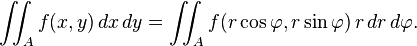
The Jacobian determinant is used when making a change of variables when evaluating a multiple integral of a function over a region within its domain. To accommodate for the change of coordinates the magnitude of the Jacobian determinant arises as a multiplicative factor within the integral. This is because the n-dimensional dV element is in general a parallelepiped in the new coordinate system, and the n-volume of a parallelepiped is the determinant of its edge vectors.
The Jacobian can also be used to solve systems of differential equations at an equilibrium point or approximate solutions near an equilibrium point.

A nonlinear map f : R2 → R2 sends a small square to a distorted parallelepiped close to the image of the square under the best linear approximation of f near the point.
According to the inverse function theorem, the matrix inverse of the Jacobian matrix of an invertible function is the Jacobian matrix of the inverse function. That is, if the Jacobian of the function f : ℝn → ℝn is continuous and nonsingular at the point p in ℝn, then f is invertible when restricted to some neighborhood of p and
The (unproved) Jacobian conjecture is related to global invertibility in the case of a polynomial functions, that is a function defined by n polynomials in n variables. It asserts that, if the Jacobian determinant is a non-zero constant (or, equivalently, that it does not have any complex zero), then the function is invertible and its inverse is a polynomial function.
If f : ℝn → ℝm is a differentiable function, a critical point of f is a point where the rank of the Jacobian matrix is not maximal. This means that the rank at the critical point is lower than the rank at some neighbour point. In other words, let k be the maximal dimension of the open balls contained in the image of f; then a point is critical if all minors of rank k of f are zero.
In the case where 1 = m = n = k, a point is critical if the Jacobian determinant is zero.
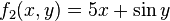
Consider the function f : ℝ2 → ℝ2 given by


![\mathbf J_{\mathbf f}(x, y) = \begin{bmatrix}
\dfrac{\partial f_1}{\partial x} & \dfrac{\partial f_1}{\partial y}\\[1em]
\dfrac{\partial f_2}{\partial x} & \dfrac{\partial f_2}{\partial y} \end{bmatrix}
= \begin{bmatrix}
2 x y & x^2 \\
5 & \cos y \end{bmatrix}](https://upload.wikimedia.org/math/7/0/d/70d7932e0a9abbebcc72e37260ec1ab1.png)
- The transformation from polar coordinates (r, φ) to Cartesian coordinates (x, y), is given by the function F: ℝ+ × [0, 2 π) → ℝ2 with components:

![\mathbf J(r, \varphi) = \begin{bmatrix}
\dfrac{\partial x}{\partial r} & \dfrac{\partial x}{\partial\varphi}\\[1em]
\dfrac{\partial y}{\partial r} & \dfrac{\partial y}{\partial\varphi} \end{bmatrix}
= \begin{bmatrix}
\cos\varphi & - r\sin \varphi \\
\sin\varphi & r\cos \varphi \end{bmatrix}](https://upload.wikimedia.org/math/b/d/0/bd068b8f6aa058df2b84641218b81466.png)

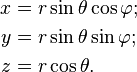
The transformation from spherical coordinates (r, θ, φ) to Cartesian coordinates (x, y, z), is given by the function F: ℝ+ × [0, π] × [0, 2 π) → ℝ3 with components:
![\mathbf J_{\mathbf F}(r, \theta, \varphi) = \begin{bmatrix}
\dfrac{\partial x}{\partial r} & \dfrac{\partial x}{\partial \theta} & \dfrac{\partial x}{\partial \varphi} \\[1em]
\dfrac{\partial y}{\partial r} & \dfrac{\partial y}{\partial \theta} & \dfrac{\partial y}{\partial \varphi} \\[1em]
\dfrac{\partial z}{\partial r} & \dfrac{\partial z}{\partial \theta} & \dfrac{\partial z}{\partial \varphi}\end{bmatrix}
= \begin{bmatrix}
\sin \theta \cos \varphi & r \cos \theta \cos \varphi & - r \sin \theta \sin \varphi \\
\sin \theta \sin \varphi & r \cos \theta \sin \varphi & r \sin \theta \cos \varphi \\
\cos \theta & - r \sin \theta & 0 \end{bmatrix}.](https://upload.wikimedia.org/math/4/7/2/472351c9d6dc5756c0a89c221ffdadca.png)
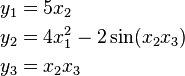
The Jacobian matrix of the function F : ℝ3 → ℝ4 with components

![\mathbf J_{\mathbf F}(x_1, x_2, x_3) = \begin{bmatrix}
\dfrac{\partial y_1}{\partial x_1} & \dfrac{\partial y_1}{\partial x_2} & \dfrac{\partial y_1}{\partial x_3} \\[1em]
\dfrac{\partial y_2}{\partial x_1} & \dfrac{\partial y_2}{\partial x_2} & \dfrac{\partial y_2}{\partial x_3} \\[1em]
\dfrac{\partial y_3}{\partial x_1} & \dfrac{\partial y_3}{\partial x_2} & \dfrac{\partial y_3}{\partial x_3} \\[1em]
\dfrac{\partial y_4}{\partial x_1} & \dfrac{\partial y_4}{\partial x_2} & \dfrac{\partial y_4}{\partial x_3} \end{bmatrix}
= \begin{bmatrix}
1 & 0 & 0 \\
0 & 0 & 5 \\
0 & 8 x_2 & -2 \\
x_3\cos x_1 & 0 & \sin x_1 \end{bmatrix}.](https://upload.wikimedia.org/math/3/2/8/3283bcdca6a874242f506371bbb7ad4a.png)
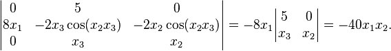
The Jacobian determinant of the function F : ℝ3 → ℝ3 with components
The Jacobian serves as a linearized design matrix in statistical regression and curve fitting; see non-linear least squares.
Dynamical systems
Consider a dynamical system of the form x′ = F(x), where x′ is the (component-wise) time derivative of x, and F : ℝn → ℝn is differentiable. If F(x0) = 0, then x0 is a stationary point (also called a critical point; this is not to be confused with fixed points). The behavior of the system near a stationary point is related to the eigenvalues of JF(x0), the Jacobian of F at the stationary point.[2] Specifically, if the eigenvalues all have real parts that are negative, then the system is stable near the stationary point, if any eigenvalue has a real part that is positive, then the point is unstable. If the largest real part of the eigenvalues is zero, the Jacobian matrix does not allow for an evaluation of the stability.Change of Variables
Back in Calculus I we had the substitution rule that told us
that,
|
|
|
In essence this is taking an integral in terms of x’s and changing it into terms of u’s.
We want to do something similar for double and triple integrals. In fact we’ve already done this to a certain
extent when we converted double integrals to polar coordinates and when we
converted triple integrals to cylindrical or spherical coordinates. The main difference is that we didn’t
actually go through the details of where the formulas came from. If you recall, in each of those cases we
commented that we would justify the formulas for dA and dV
eventually. Now is the time to do that
justification.
While often the reason for changing variables is to
get us
an integral that we can do with the new variables, another reason for
changing
variables is to convert the region into a nicer region to work with.
When we were converting the polar, cylindrical
or spherical coordinates we didn’t worry about this change since it was
easy
enough to determine the new limits based on the given region. That is
not always the case however. So, before we move into changing variables
with multiple integrals we first need to see how the region may change
with a
change of variables.
First we need a little notation out of the way. We call the equations that define the change
of variables a transformation. Also we will typically start out with a
region, R, in xy-coordinates and transform it into a region in uv-coordinates.
|
Example 1 Determine
the new region that we get by applying the given transformation to the region
R.
Solution
There really isn’t too much to do with this one other than
to plug the transformation into the equation for the ellipse and see what we
get.
 
So, we started out with an ellipse and after the
transformation we had a disk of radius 2.
As with the first part we’ll need to plug the
transformation into the equation, however, in this case we will need to do it
three times, once for each equation.
Before we do that let’s sketch the graph of the region and see what
we’ve got.
|


So, we have a triangle.
Now, let’s go through the transformation. We will apply the transformation to each
edge of the triangle and see where we get.
Let’s do 


The first boundary transforms very nicely into a much
simpler equation.
Now let’s take a look at 


Again, a much nicer equation that what we started with.
Finally, let’s transform 


So, again, we got a somewhat simpler equation, although
not quite as nice as the first two.
Let’s take a look at the new region that we get under the
transformation.

We still get a triangle, but a much nicer one.
Note that we can’t always expect to transform a specific
type of region (a triangle for example) into the same kind of region. It is completely possible to have a triangle
transform into a region in which each of the edges are curved and in no way
resembles a triangle.
Notice that in each of the above examples we took a two
dimensional region that would have been somewhat difficult to integrate over
and converted it into a region that would be much nicer in integrate over. As we noted at the start of this set of
examples, that is often one of the points behind the transformation. In addition to converting the integrand into
something simpler it will often also transform the region into one that is much
easier to deal with.
Now that we’ve seen a couple of examples of transforming
regions we need to now talk about how we actually do change of variables in the
integral. We will start with double
integrals. In order to change variables
in a double integral we will need the Jacobian
of the transformation. Here is the definition
of the Jacobian.
Definition
|
The Jacobian of
the transformation
  |
The Jacobian is defined as a determinant of a 2x2 matrix, if
you are unfamiliar with this that is okay.
Here is how to compute the determinant.
 |
|
Therefore, another formula for the determinant is,
  |
|
Now that we have the Jacobian out of the way we can give the
formula for change of variables for a double integral.
Tidak ada komentar:
Posting Komentar