In daily activities we know the title of clock or scheduling in the running time.
Electronics components are known as 555 tesla integrated circuit wire
Timer (Self-timer)
INTERCOM WITH 555 TESLA COUNT ROLLING ( CONTROLL )
Timer
Timer circuit is a series of multivibrator (frequency / pulse generator) where we can control the time to turn on or off. IC NE 555 is an example of a timer IC (timer). This series of groups is used to correctly determine the time delay. Unlike op amp741, this tool can only provide high or low output voltages.
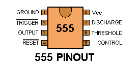
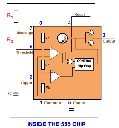
IC NE 555 has 8 pins with the following Physical Conditions

Note:
1.The tension For Vcc foot is between 5-12 V
2. foot No2 (trigger) is active low so to enable should be given zero logic
3. Feet No. 4 (reset) is a foot with low active condition, so if exposed to logic LOW IC will restart, and in circuit usually connected to VCC
4.output is at the foot no 3
There are two types of 555 ie IC work as
Monostable circuit or as astable circuit.
Timer monostable Multivibrator

Work principle :
- Monostabil means he will only be setabil when fired (in trigger). On the use of this ignition can use SW1, when it is released then the triger active and led will be on for a certain time. Or the input can use a touch of the hand, the led will light up for a time equal to the R and C values.
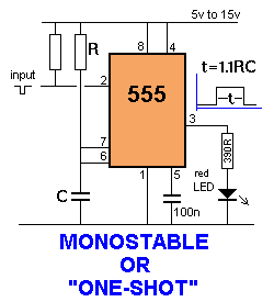
- The length of time the output is in high condition is determined by the magnitude of the values of the C1 and the resistor R1. The width of the pulse is a time interval when the output voltage is high. For the circuit shown in the figure, the width of the T pulse is given by the equation
T = 1.1 x R2 x C1
- keep in mind that trigger is active LOW
-The pulse diagram of the input and output relationships is illustrated

Timer for Multivibrator A Stable

monostable Multivibrator
555 timer chip tester

IC 555 timer tester is a simple circuit that serves to test the condition of IC 555. 555 timer circuit tester, in principle, start the timer 555 in astable multivibrator mode. As an indicator of the status of the timer 555 good condition or damaged to use 2 pieces LED which will light up in a blink alternately when the timer 555 in good condition.
And only one will turn on or off all the timer 555 when the condition is broken. 555 timer circuit tester is powered using 9 Volt DC voltage source. Complete circuit tester 555 as follows.
 |
| Tester schematic |
How to use 555 timer tester is in conjunction with IC 555 to test the existing IC socket according to the order button. Then activate the power switch to begin testing the 555 timer IC. Then live we observe the LED indicators 2buah before, whether flashing alternately (good) or not blink or even die all (timer 555 damaged).
 The servo motor tester circuit
 How to use IC 555 tesla
THE 555 The 555 is everywhere. It is possibly the most-frequency used chip and is easy to use.
But if you want to use it in a "one-shot" or similar circuit, you need to know how the chip will "sit."
For this you need to know about the UPPER THRESHOLD (pin 6) and LOWER THRESHOLD (pin 2):
The 555 is fully covered in a 3 page article on Talking Electronics website (see left index: 555 P1 P2 P3)
Here is the pin identification for each pin:
When drawing a circuit diagram, always draw the 555 as a building block with the pins in the following locations. This will help you instantly recognise the function of each pin:
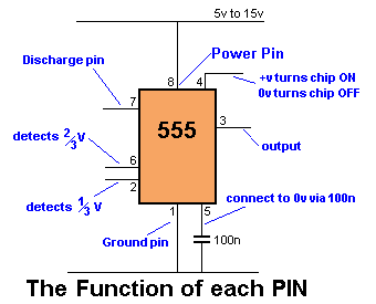
Note: Pin 7 is "in phase" with output Pin 3 (both are low at the same time).
Pin 7 "shorts" to 0v via the transistor. It is pulled HIGH via R1.
Maximum supply voltage 16v - 18v
Current consumption approx 10mA
Output Current sink @5v = 5 - 50mA @15v = 50mA
Output Current source @5v = 100mA @15v = 200mA
Maximum operating frequency 300kHz - 500kHz
Faults with Chip:
Consumes about 10mA when sitting in circuit
Output voltage up to 2.5v less than rail voltage
Output is 0.5v to 1.5v above ground
Sources up to 200mA but sinks only 50mA
HOW TO USE THE 555
There are many ways to use the 55.
(a) Astable Multivibrator - constantly oscillates
(b) Monostable - changes state only once per trigger pulse - also called a ONE SHOT
(c) Voltage Controlled Oscillator
ASTABLE MULTIVIBRATOR The output frequency of a 555 can be worked out from the following graph:
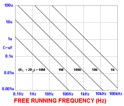
The graph applies to the following Astable circuit:
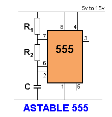 | The capacitor C charges via R1 and R2 and when the voltage on the capacitor reaches 2/3 of the supply, pin 6 detects this and pin 7 connects to 0v. The capacitor discharges through R2 until its voltage is 1/3 of the supply and pin 2 detects this and turns off pin7 to repeat the cycle. The top resistor is included to prevent pin 7 being damaged as it shorts to 0v when pin 6 detects 2/3 rail voltage. Its resistance is small compared to R2 and does not come into the timing of the oscillator. |
Using the graph:
Suppose R1 = 1k, R2 = 10k and C = 0.1 (100n).
Using the formula on the graph, the total resistance = 1 + 10 + 10 = 21k
The scales on the graph are logarithmic so that 21k is approximately near the "1" on the 10k. Draw a line parallel to the lines on the graph and where it crosses the 0.1u line, is the answer. The result is approx 900Hz.
Suppose R1 = 10k, R2 = 100k and C = 1u
Using the formula on the graph, the total resistance = 10 + 100 + 100 = 210k
The scales on the graph are logarithmic so that 210k is approximately near the first "0" on the 100k. Draw a line parallel to the lines on the graph and where it crosses the 1u line, is the answer. The result is approx 9Hz.
The frequency of an astable circuit can also be worked out from the following formula:
| frequency = | 1.4 |
| (R1 + 2R2) × C |
| ||||||||||||||||||||||||||||
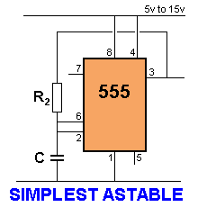 | The simplest Astable uses one resistor and one capacitor. Output pin 3 is used to charge and discharge the capacitor. |
| LOW FREQUENCY OSCILLATORS | |
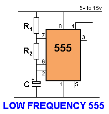 | If the capacitor is replaced with an electrolytic, the frequency of oscillation will reduce. When the frequency is less than 1Hz, the oscillator circuit is called a timer or "delay circuit." The 555 will produce delays as long as 30 minutes but with long delays, the timing is not accurate. |
| ||||||||||||||||||||
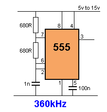
Here are circuits that operate from 300kHz to 30 minutes:
(300kHz is the absolute maximum as the 555 starts to malfunction with irregular bursts of pulses at this high frequency and 30 minutes is about the longest you can guarantee the cycle will repeat.)
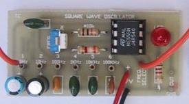
 SQUARE WAVE OSCILLATOR
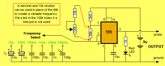
A square wave oscillator kit can be purchased from Talking Electronics for approx $10.00
See website: Square Wave OscillatorIt has adjustable (and settable) frequencies from 1Hz to 100kHz and is an ideal piece of Test Equipment.
555 Monostable or "one Shot"
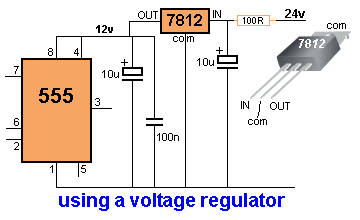
 USING A VOLTAGE REGULATORThis circuit shows how to use a voltage regulator to convert a 24v supply to 12v for a 555 chip. Note: the pins on the regulator (commonly called a 3-terminal regulator) are: IN, COMMON, OUT and these must match-up with: In, Common, Out on the circuit diagram.
 If the current requirement is less than 500mA, a 100R "safety resistor" can be placed on the 24v rail to prevent spikes damaging the regulator.
| POLICE LIGHTS These three circuits flash the left LEDs 3 times then the right LEDs 3 times, then repeats. The only difference is the choice of chips. 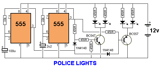 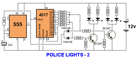 |
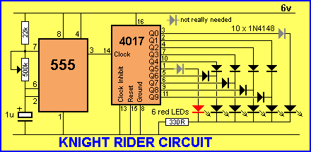
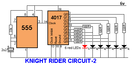
KNIGHT RIDERIn the Knight Rider circuit, the 555 is wired as an oscillator. It can be adjusted to give the desired speed for the display. The output of the 555 is directly connected to the input of a Johnson Counter (CD 4017). The input of the counter is called the CLOCK line.
The 10 outputs Q0 to Q9 become active, one at a time, on the rising edge of the waveform from the 555. Each output can deliver about 20mA but a LED should not be connected to the output without a current-limiting resistor (330R in the circuit above).
The first 6 outputs of the chip are connected directly to the 6 LEDs and these "move" across the display. The next 4 outputs move the effect in the opposite direction and the cycle repeats. The animation above shows how the effect appears on the display.
Using six 3mm LEDs, the display can be placed in the front of a model car to give a very realistic effect. The same outputs can be taken to driver transistors to produce a larger version of the display.
Here is a simple Knight Rider circuit using resistors to drive the LEDs. This circuit consumes 22mA while only delivering 7mA to each LED. The outputs are "fighting" each other via the 100R resistors (except outputs Q0 and Q5).
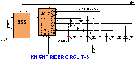
This circuit drives 11 LEDs with a cross-over effect:

KNIGHT RIDER "RUNNING HOLE" EFFECT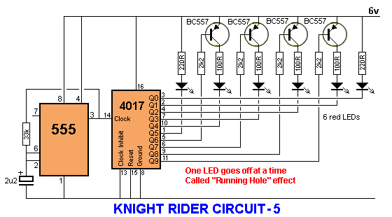

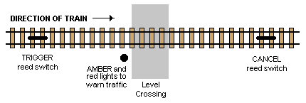
CROSSING LIGHTS
A magnet on the train activates the TRIGGER reed switch to turn on the amber LED for a time determined by the value of the first 10u and 47k.
When the first 555 IC turns off, the 100n is uncharged because both ends are at rail voltage and it pulses pin 2 of the middle 555 LOW. This activates the 555 and pin 3 goes HIGH. This pin supplies rail voltage to the third 555 and the two red LEDs are alternately flashed. When the train passes the CANCEL reed switch, pin 4 of the middle 555 is taken LOW and the red LEDs stop flashing.
See it in action: Movie (4MB)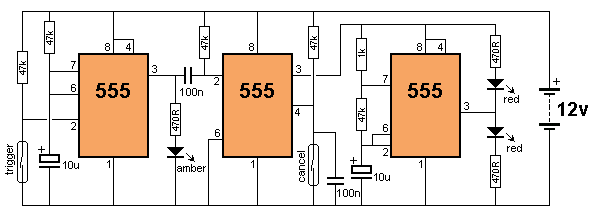
 KNIGHT RIDER "RUNNING HOLE" EFFECT
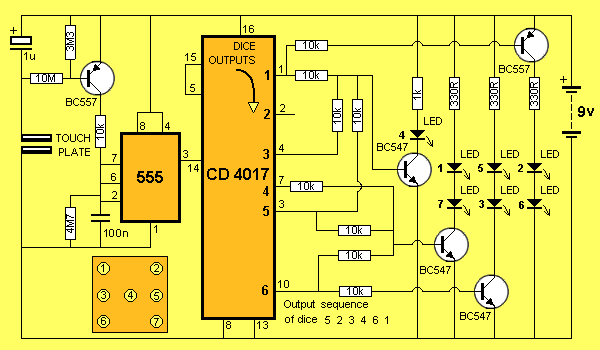
LED DICE
This circuit produces a realistic effect of the "pips" on the face of a dice. The circuit has "slow-down" to give the effect of the dice "rolling."
See the full project: LED DICE
A SIMPLER CIRCUIT:
The circuit above can be simplified and output Pin 12 can be used to illuminate two of the LEDs as this line is HIGH for the times when Q0, Q1, Q2, Q3, and Q4 are HIGH and goes LOW when Q5 - Q9 is HIGH.
This means the 4017 starts with Q0 HIGH. But Q0 is not an output. This means that when Q0 is HIGH, "carry out" is HIGH and "2" will be displayed. The next clock cycle will produce "3" on the display when Q1 is HIGH, then "4" when Q2 is HIGH, "5" when Q3 is HIGH and "6" when Q4 is HIGH. When Q5 goes HIGH, it illuminates "1" on the display because "carry out" goes LOW.
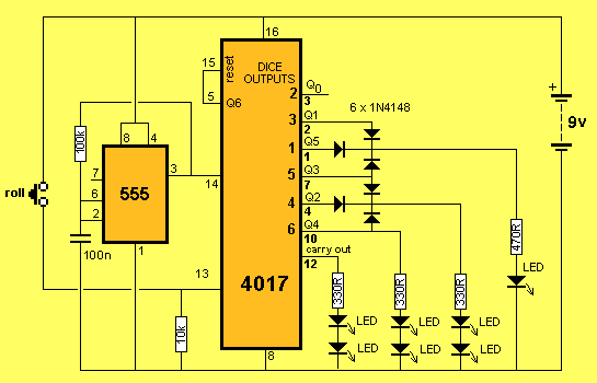 LED DICE - minimum components
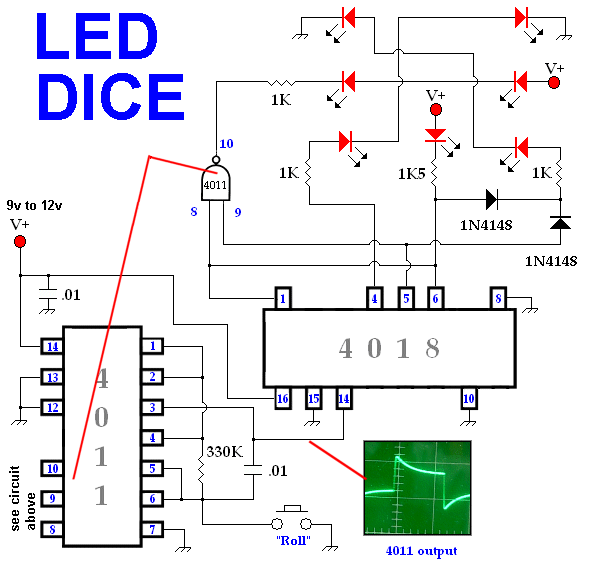 LED DICE - using CD4018 5-bit Counter
X . I
ELECTRONIC SYSTEM COUNT ROLLING ( CONTROLL )

It does this with the aid of input devices such as sensors, that respond in some way to this information and then uses electrical energy in the form of an output action to control a physical process or perform some type of mathematical operation on the signal.
But electronic control systems can also be regarded as a process that transforms one signal into another so as to give the desired system response. Then we can say that a simple electronic system consists of an input, a process, and an output with the input variable to the system and the output variable from the system both being signals.
There are many ways to represent a system, for example: mathematically, descriptively, pictorially or schematically. Electronic systems are generally represented schematically as a series of interconnected blocks and signals with each block having its own set of inputs and outputs.
As a result, even the most complex of electronic control systems can be represented by a combination of simple blocks, with each block containing or representing an individual component or complete sub-system. The representing of an electronic system or process control system as a number of interconnected blocks or boxes is known commonly as “block-diagram representation”.
 Electronic Systems have both inputs and outputs with the output or outputs being produced by processing the inputs. Also, the input signal(s) may cause the process to change or may itself cause the operation of the system to change. Therefore the input(s) to a system is the “cause” of the change, while the resulting action that occurs on the systems output due to this cause being present is called the “effect”, with the effect being a consequence of the cause.
In other words, an electronic system can be classed as “causal” in nature as there is a direct relationship between its input and its output. Electronic systems analysis and process control theory are generally based upon this Cause and Effect analysis.
So for example in an audio system, a microphone (input device) causes sound waves to be converted into electrical signals for the amplifier to amplify (a process), and a loudspeaker (output device) produces sound waves as an effect of being driven by the amplifiers electrical signals.
But an electronic system need not be a simple or single operation. It can also be an interconnection of several sub-systems all working together within the same overall system.
Our audio system could for example, involve the connection of a CD player, or a DVD player, an MP3 player, or a radio receiver all being multiple inputs to the same amplifier which in turn drives one or more sets of stereo or home theatre type surround loudspeakers.
But an electronic system can not just be a collection of inputs and outputs, it must “do something”, even if it is just to monitor a switch or to turn “ON” a light. We know that sensors are input devices that detect or turn real world measurements into electronic signals which can then be processed. These electrical signals can be in the form of either voltages or currents within a circuit. The opposite or output device is called an actuator, that converts the processed signal into some operation or action, usually in the form of mechanical movement.
But a continuous-time signal can also vary in magnitude or be periodic in nature with a time period T. As a result, continuous-time electronic systems tend to be purely analogue systems producing a linear operation with both their input and output signals referenced over a set period of time.
 For example, the temperature of a room can be classed as a continuous time signal which can be measured between two values or set points, for example from cold to hot or from Monday to Friday. We can represent a continuous-time signal by using the independent variable for time t, and where x(t) represents the input signal and y(t) represents the output signal over a period of time t.
Generally, most of the signals present in the physical world which we can use tend to be continuous-time signals. For example, voltage, current, temperature, pressure, velocity, etc.
On the other hand, a discrete-time system is one in which the input signals are not continuous but a sequence or a series of signal values defined in “discrete” points of time. This results in a discrete-time output generally represented as a sequence of values or numbers.
Generally a discrete signal is specified only at discrete intervals, values or equally spaced points in time. So for example, the temperature of a room measured at 1pm, at 2pm, at 3pm and again at 4pm without regards for the actual room temperature in between these points at say, 1:30pm or at 2:45pm.
 However, a continuous-time signal, x(t) can be represented as a discrete set of signals only at discrete intervals or “moments in time”. Discrete signals are not measured versus time, but instead are plotted at discrete time intervals, where n is the sampling interval. As a result discrete-time signals are usually denoted as x(n) representing the input and y(n) representing the output.
Then we can represent the input and output signals of a system as x and y respectively with the signal, or signals themselves being represented by the variable, t, which usually represents time for a continuous system and the variable n, which represents an integer value for a discrete system as shown.

When subsystems are combined to form a series circuit, the overall output at y(t) will be equivalent to the multiplication of the input signal x(t) as shown as the subsystems are
cascaded together.
 For a series connected continuous-time system, the output signal y(t) of the first subsystem, “A” becomes the input signal of the second subsystem, “B” whose output becomes the input of the third subsystem, “C” and so on through the series chain giving A x B x C, etc.
Then the original input signal is cascaded through a series connected system, so for two series connected subsystems, the equivalent single output will be equal to the multiplication of the systems, ie, y(t) = G1(s) x G2(s). Where G represents the transfer function of the subsystem.
Note that the term “Transfer Function” of a system refers to and is defined as being the mathematical relationship between the systems input and its output, or output/input and hence describes the behaviour of the system.
Also, for a series connected system, the order in which a series operation is performed does not matter with regards to the input and output signals as: G1(s) x G2(s) is the same as G2(s) x G1(s). An example of a simple series connected circuit could be a single microphone feeding an amplifier followed by a speaker.
 For a parallel connected continuous-time system, each subsystem receives the same input signal, and their individual outputs are summed together to produce an overall output, y(t). Then for two parallel connected subsystems, the equivalent single output will be the sum of the two individual inputs, ie, y(t) = G1(s) + G2(s).
An example of a simple parallel connected circuit could be several microphones feeding into a mixing desk which in turn feeds an amplifier and speaker system.
 Feedback systems are used a lot in most practical electronic system designs to help stabilise the system and to increase its control. If the feedback loop reduces the value of the original signal, the feedback loop is known as “negative feedback”. If the feedback loop adds to the value of the original signal, the feedback loop is known as “positive feedback”.
An example of a simple feedback system could be a thermostatically controlled heating system in the home. If the home is too hot, the feedback loop will switch “OFF” the heating system to make it cooler. If the home is too cold, the feedback loop will switch “ON” the heating system to make it warmer. In this instance, the system comprises of the heating system, the air temperature and the thermostatically controlled feedback loop.
 Any subsystem can be represented as a simple block with an input and output as shown. Generally, the input is designated as: θi and the output as: θo. The ratio of output over input represents the gain, ( G ) of the subsystem and is therefore defined as: G = θo/θi
In this case, G represents the Transfer Function of the system or subsystem. When discussing electronic systems in terms of their transfer function, the complex operator, s is used, then the equation for the gain is rewritten as: G(s) = θo(s)/θi(s)
Block diagrams need not represent a simple single system but can represent very complex systems made from many interconnected subsystems. These subsystems can be connected together in series, parallel or combinations of both depending upon the flow of the signals.
We have also seen that electronic signals and systems can be of continuous-time or discrete-time in nature and may be analogue, digital or both. Feedback loops can be used be used to increase or reduce the performance of a particular system by providing better stability and control. Control is the process of making a system variable adhere to a particular value, called the reference value.
Understanding And Excess Microcontroller
Microcontroller, as a breakthrough microprocessor technology and microcomputer is a new technology to meet market needs. Microcontroller as a new technology, semiconductor technology with more transistor content but requires only a small space so that microcontroller can be mass produced (in large quantities) make the price cheaper (compared to microprocessors). Microcontroller as a market need, microcontroller is present to meet the tastes of industry and consumers will the needs and desires of tools and toys even better and more sophisticated.
Unlike computer systems, capable of handling a variety of application programs (eg word processing, number processing and so on), microcontrollers can only be used for a particular application (only one program can be stored). Another difference lies in the ratio of RAM and ROM. In computer systems the ratio of RAM and ROM is large, meaning that user programs are stored in relatively large RAM space, while hardware interface routines are stored in small ROM spaces. While on the Microcontroller, the ratio of ROM and RAM is large, it means that the control program is stored in ROM (can Masked ROM or Flash PEROM) which is relatively larger, while RAM is used as a temporary storage, including the registers used in microcontroller Concerned
There are several members of microcontroller MCS51 that has internal memory, one of them is microcontroller AT89C51 which is EEPROM version of 80C51 where this internal memory can be programmed and removed electrically and produced by ATMEL Corporation. AT89C51 is made compatible with the MCS-51 standard industrial output and output cells that have 4Kbyte of internal RAM with EEPROM flash technology that can store data even when the power supply is turned off.
The MCS-51 family is an 8 bit microcontroller as shown in the following table:
X . II
OPEN LOOP SYSTEM

Likewise, if something happens to disturb the systems output without any change to the input value, the output must respond by returning back to its previous set value. In the past, electrical control systems were basically manual or what is called an Open-loop System with very few automatic control or feedback features built in to regulate the process variable so as to maintain the desired output level or value.
For example, an electric clothes dryer. Depending upon the amount of clothes or how wet they are, a user or operator would set a timer (controller) to say 30 minutes and at the end of the 30 minutes the drier will automatically stop and turn-off even if the clothes are still wet or damp.
In this case, the control action is the manual operator assessing the wetness of the clothes and setting the process (the drier) accordingly.
So in this example, the clothes dryer would be an open-loop system as it does not monitor or measure the condition of the output signal, which is the dryness of the clothes. Then the accuracy of the drying process, or success of drying the clothes will depend on the experience of the user (operator).
However, the user may adjust or fine tune the drying process of the system at any time by increasing or decreasing the timing controllers drying time, if they think that the original drying process will not be met. For example, increasing the timing controller to 40 minutes to extend the drying process. Consider the following open-loop block diagram.
 Then an Open-loop system, also referred to as non-feedback system, is a type of continuous control system in which the output has no influence or effect on the control action of the input signal. In other words, in an open-loop control system the output is neither measured nor “fed back” for comparison with the input. Therefore, an open-loop system is expected to faithfully follow its input command or set point regardless of the final result.
Also, an open-loop system has no knowledge of the output condition so cannot self-correct any errors it could make when the preset value drifts, even if this results in large deviations from the preset value.
Another disadvantage of open-loop systems is that they are poorly equipped to handle disturbances or changes in the conditions which may reduce its ability to complete the desired task. For example, the dryer door opens and heat is lost. The timing controller continues regardless for the full 30 minutes but the clothes are not heated or dried at the end of the drying process. This is because there is no information fed back to maintain a constant temperature.
 Then we can see that open-loop system errors can disturb the drying process and therefore requires extra supervisory attention of a user (operator). The problem with this anticipatory control approach is that the user would need to look at the process temperature frequently and take any corrective control action whenever the drying process deviated from its desired value of drying the clothes. This type of manual open-loop control which reacts before an error actually occurs is called Feed forward Control
The objective of feed forward control, also known as predictive control, is to measure or predict any potential open-loop disturbances and compensate for them manually before the controlled variable deviates too far from the original set point. So for our simple example above, if the dryers door was open it would be detected and closed allowing the drying process to continue.
 If applied correctly, the deviation from wet clothes to dry clothes at the end of the 30 minutes would be minimal if the user responded to the error situation (door open) very quickly. However, this feed forward approach may not be completely accurate if the system changes, for example the drop in drying temperature was not noticed during the 30 minute process.
Then we can define the main characteristics of an “Open-loop system” as being:
Generally, we do not have to manipulate the open-loop block diagram to calculate its actual transfer function. We can just write down the proper relationships or equations from each block diagram, and then calculate the final transfer function from these equations as shown.
 The Transfer Function of each block is:
 The overall transfer function is:
 Then the Open-loop Gain is given simply as:
 When G represents the Transfer Function of the system or subsystem, it can be rewritten as: G(s) = θo(s)/θi(s)
Open-loop control systems are often used with processes that require the sequencing of events with the aid of “ON-OFF” signals. For example a washing machines which requires the water to be switched “ON” and then when full is switched “OFF” followed by the heater element being switched “ON” to heat the water and then at a suitable temperature is switched “OFF”, and so on.
This type of “ON-OFF” open-loop control is suitable for systems where the changes in load occur slowly and the process is very slow acting, necessitating infrequent changes to the control action by an operator.
An “open-loop system” is defined by the fact that the output signal or condition is neither measured nor “fed back” for comparison with the input signal or system set point. Therefore open-loop systems are commonly referred to as “Non-feedback systems”.
Also, as an open-loop system does not use feedback to determine if its required output was achieved, it “assumes” that the desired goal of the input was successful because it cannot correct any errors it could make, and so cannot compensate for any external disturbances to the system.
 If the potentiometer is moved to the top of the resistance the maximum positive voltage will be supplied to the amplifier representing full speed. Likewise, if the potentiometer wiper is moved to the bottom of the resistance, zero voltage will be supplied representing a very slow speed or stop.
Then the position of the potentiometers slider represents the input, θi which is amplified by the amplifier (controller) to drive the DC motor (process) at a set speed N representing the output, θo of the system. The motor will continue to rotate at a fixed speed determined by the position of the potentiometer.
As the signal path from the input to the output is a direct path not forming part of any loop, the overall gain of the system will the cascaded values of the individual gains from the potentiometer, amplifier, motor and load. It is clearly desirable that the output speed of the motor should be identical to the position of the potentiometer, giving the overall gain of the system as unity.
However, the individual gains of the potentiometer, amplifier and motor may vary over time with changes in supply voltage or temperature, or the motors load may increase representing external disturbances to the open-loop motor control system.
But the user will eventually become aware of the change in the systems performance (change in motor speed) and may correct it by increasing or decreasing the potentiometers input signal accordingly to maintain the original or desired speed.
The advantages of this type of “open-loop motor control” is that it is potentially cheap and simple to implement making it ideal for use in well-defined systems were the relationship between input and output is direct and not influenced by any outside disturbances. Unfortunately this type of open-loop system is inadequate as variations or disturbances in the system affect the speed of the motor. Then another form of control is required.

But the goal of any electrical or electronic control system is to measure, monitor, and control a process and one way in which we can accurately control the process is by monitoring its output and “feeding” some of it back to compare the actual output with the desired output so as to reduce the error and if disturbed, bring the output of the system back to the original or desired response.
The quantity of the output being measured is called the “feedback signal”, and the type of control system which uses feedback signals to both control and adjust itself is called a Close-loop System.
A Closed-loop Control System, also known as a feedback control system is a control system which uses the concept of an open loop system as its forward path but has one or more feedback loops (hence its name) or paths between its output and its input. The reference to “feedback”, simply means that some portion of the output is returned “back” to the input to form part of the systems excitation.
Closed-loop systems are designed to automatically achieve and maintain the desired output condition by comparing it with the actual condition. It does this by generating an error signal which is the difference between the output and the reference input. In other words, a “closed-loop system” is a fully automatic control system in which its control action being dependent on the output in some way.
So for example, consider our electric clothes dryer from the previous open-loop tutorial. Suppose we used a sensor or transducer (input device) to continually monitor the temperature or dryness of the clothes and feed a signal relating to the dryness back to the controller as shown below.
 This sensor would monitor the actual dryness of the clothes and compare it with (or subtract it from) the input reference. The error signal (error = required dryness – actual dryness) is amplified by the controller, and the controller output makes the necessary correction to the heating system to reduce any error. For example if the clothes are too wet the controller may increase the temperature or drying time. Likewise, if the clothes are nearly dry it may reduce the temperature or stop the process so as not to overheat or burn the clothes, etc.
Then the closed-loop configuration is characterised by the feedback signal, derived from the sensor in our clothes drying system. The magnitude and polarity of the resulting error signal, would be directly related to the difference between the required dryness and actual dryness of the clothes.
Also, because a closed-loop system has some knowledge of the output condition, (via the sensor) it is better equipped to handle any system disturbances or changes in the conditions which may reduce its ability to complete the desired task.
For example, as before, the dryer door opens and heat is lost. This time the deviation in temperature is detected by the feedback sensor and the controller self-corrects the error to maintain a constant temperature within the limits of the preset value. Or possibly stops the process and activates an alarm to inform the operator.
As we can see, in a closed-loop control system the error signal, which is the difference between the input signal and the feedback signal (which may be the output signal itself or a function of the output signal), is fed to the controller so as to reduce the systems error and bring the output of the system back to a desired value. In our case the dryness of the clothes. Clearly, when the error is zero the clothes are dry.
The term Closed-loop control always implies the use of a feedback control action in order to reduce any errors within the system, and its “feedback” which distinguishes the main differences between an open-loop and a closed-loop system.The accuracy of the output thus depends on the feedback path, which in general can be made very accurate and within electronic control systems and circuits, feedback control is more commonly used than open-loop or feed forward control.
Closed-loop systems have many advantages over open-loop systems. The primary advantage of a closed-loop feedback control system is its ability to reduce a system’s sensitivity to external disturbances, for example opening of the dryer door, giving the system a more robust control as any changes in the feedback signal will result in compensation by the controller.
Then we can define the main characteristics of Closed-loop Control as being:
 CROSS A NEW TESTAMENT PID / PITa memory flyer
The symbol used to represent a summing point in closed-loop systems block-diagram is that of a circle with two crossed lines as shown. The summing point can either add signals together in which a Plus ( + ) symbol is used showing the device to be a “summer” (used for positive feedback), or it can subtract signals from each other in which case a Minus ( − ) symbol is used showing that the device is a “comparator” (used for negative feedback) as shown.
CROSS A NEW TESTAMENT PID / PITa memory flyer
The symbol used to represent a summing point in closed-loop systems block-diagram is that of a circle with two crossed lines as shown. The summing point can either add signals together in which a Plus ( + ) symbol is used showing the device to be a “summer” (used for positive feedback), or it can subtract signals from each other in which case a Minus ( − ) symbol is used showing that the device is a “comparator” (used for negative feedback) as shown.
 Note that summing points can have more than one signal as inputs either adding or subtracting but only one output which is the algebraic sum of the inputs. Also the arrows indicate the direction of the signals. Summing points can be cascaded together to allow for more input variables to be summed at a given point.
 Where: block G represents the open-loop gains of the controller or system and is the forward path, and block H represents the gain of the sensor, transducer or measurement system in the feedback path.
To find the transfer function of the closed-loop system above, we must first calculate the output signal θo in terms of the input signal θi. To do so, we can easily write the equations of the given block-diagram as follows.
The output from the system is equal to: Output = G x Error
Note that the error signal, θe is also the input to the feed-forward block: G
The output from the summing point is equal to: Error = Input - H x Output
If H = 1 (unity feedback) then:
The output from the summing point will be: Error (θe) = Input - Output
Eliminating the error term, then:
The output is equal to: Output = G x (Input - H x Output)
Therefore: G x Input = Output + G x H x Output
Rearranging the above gives us the closed-loop transfer function of:
 The above equation for the transfer function of a closed-loop system shows a Plus ( + ) sign in the denominator representing negative feedback. With a positive feedback system, the denominator will have a Minus ( − ) sign and the equation becomes: 1 - GH.
We can see that when H = 1 (unity feedback) and G is very large, the transfer function approaches unity as:
 Also, as the systems steady state gain G decreases, the expression of: G/(1 + G) decreases much more slowly. In other words, the system is fairly insensitive to variations in the systems gain represented by G, and which is one of the main advantages of a closed-loop system.
Consider the multi-loop system below.
 Any cascaded blocks such as G1 and G2 can be reduced, as well as the transfer function of the inner loop as shown.
 After further reduction of the blocks we end up with a final block diagram which resembles that of the previous single-loop closed-loop system.
 And the transfer function of this multi-loop system becomes:
 Then we can see that even complex multi-block or multi-loop block diagrams can be reduced to give one single block diagram with one common system transfer function.
Then the position of the potentiometers slider represents the input, θi which is amplified by the amplifier (controller) to drive the DC motor at a set speed N representing the output, θo of the system, and the tachometer T would be the closed-loop back to the controller. The difference between the input voltage setting and the feedback voltage level gives the error signal as shown.
 Any external disturbances to the closed-loop motor control system such as the motors load increasing would create a difference in the actual motor speed and the potentiometer input set point.
This difference would produce an error signal which the controller would automatically respond too adjusting the motors speed. Then the controller works to minimize the error signal, with zero error indicating actual speed which equals set point.
Electronically, we could implement such a simple closed-loop tachometer-feedback motor control circuit using an operational amplifier (op-amp) for the controller as shown.
 This simple closed-loop motor controller can be represented as a block diagram as shown.
 A closed-loop motor controller is a common means of maintaining a desired motor speed under varying load conditions by changing the average voltage applied to the input from the controller. The tachometer could be replaced by an optical encoder or Hall-effect type positional or rotary sensor.
In a closed-loop system, a controller is used to compare the output of a system with the required condition and convert the error into a control action designed to reduce the error and bring the output of the system back to the desired response. Then closed-loop control systems use feedback to determine the actual input to the system and can have more than one feedback loop.
Closed-loop control systems have many advantages over open-loop systems. One advantage is the fact that the use of feedback makes the system response relatively insensitive to external disturbances and internal variations in system parameters such as temperature. It is thus possible to use relatively inaccurate and inexpensive components to obtain the accurate control of a given process or plant.
However, system stability can be a major problem especially in badly designed closed-loop systems as they may try to over-correct any errors which could cause the system to loss control and oscillate.
In the next tutorial about Electronics Systems, we will look at the different ways in which we can incorporate a summing point into the input of a system and the different ways in which we can feed signals back to it.

Simple analogue feedback control circuits can be constructed using individual or discrete components, such as transistors, resistors and capacitors, etc, or by using microprocessor-based and integrated circuits (IC’s) to form more complex digital feedback systems.
As we have seen, open-loop systems are just that, open ended, and no attempt is made to compensate for changes in circuit conditions or changes in load conditions due to variations in circuit parameters, such as gain and stability, temperature, supply voltage variations and/or external disturbances. But the effects of these “open-loop” variations can be eliminated or at least considerably reduced by the introduction of Feedback.
A feedback system is one in which the output signal is sampled and then fed back to the input to form an error signal that drives the system. In the previous tutorial about Closed-loop Systems, we saw that in general, feedback is comprised of a sub-circuit that allows a fraction of the output signal from a system to modify the effective input signal in such a way as to produce a response that can differ substantially from the response produced in the absence of such feedback.
Feedback Systems are very useful and widely used in amplifier circuits, oscillators, process control systems as well as other types of electronic systems. But for feedback to be an effective tool it must be controlled as an uncontrolled system will either oscillate or fail to function. The basic model of a feedback system is given as:
 This basic feedback loop of sensing, controlling and actuation is the main concept behind a feedback control system and there are several good reasons why feedback is applied and used in electronic circuits:
However, in electronic and control systems to much praise and positive feedback can increase the systems gain far too much which would give rise to oscillatory circuit responses as it increases the magnitude of the effective input signal.
An example of a positive feedback systems could be an electronic amplifier based on an operational amplifier, or op-amp as shown.
 Positive feedback control of the op-amp is achieved by applying a small part of the output voltage signal at Vout back to the non-inverting ( + ) input terminal via the feedback resistor, RF.
If the input voltage Vin is positive, the op-amp amplifies this positive signal and the output becomes more positive. Some of this output voltage is returned back to the input by the feedback network.
Thus the input voltage becomes more positive, causing an even larger output voltage and so on. Eventually the output becomes saturated at its positive supply rail.
Likewise, if the input voltage Vin is negative, the reverse happens and the op-amp saturates at its negative supply rail. Then we can see that positive feedback does not allow the circuit to function as an amplifier as the output voltage quickly saturates to one supply rail or the other, because with positive feedback loops “more leads to more” and “less leads to less”.
Then if the loop gain is positive for any system the transfer function will be: Av = G / (1 – GH). Note that if GH = 1 the system gain Av = infinity and the circuit will start to self-oscillate, after which no input signal is needed to maintain oscillations, which is useful if you want to make an oscillator.
Although often considered undesirable, this behaviour is used in electronics to obtain a very fast switching response to a condition or signal. One example of the use of positive feedback is hysteresis in which a logic device or system maintains a given state until some input crosses a preset threshold. This type of behaviour is called “bi-stability” and is often associated with logic gates and digital switching devices such as multivibrators.
We have seen that positive or regenerative feedback increases the gain and the possibility of instability in a system which may lead to self-oscillation and as such, positive feedback is widely used in oscillatory circuits such as Oscillators and Timing circuits.
Because negative feedback produces stable circuit responses, improves stability and increases the operating bandwidth of a given system, the majority of all control and feedback systems is degenerative reducing the effects of the gain.
An example of a negative feedback system is an electronic amplifier based on an operational amplifier as shown.
 Negative feedback control of the amplifier is achieved by applying a small part of the output voltage signal at Vout back to the inverting ( – ) input terminal via the feedback resistor, Rf.
If the input voltage Vin is positive, the op-amp amplifies this positive signal, but because its connected to the inverting input of the amplifier, and the output becomes more negative. Some of this output voltage is returned back to the input by the feedback network of Rf.
Thus the input voltage is reduced by the negative feedback signal, causing an even smaller output voltage and so on. Eventually the output will settle down and become stabilised at a value determined by the gain ratio of Rf ÷ Rin.
Likewise, if the input voltage Vin is negative, the reverse happens and the op-amps output becomes positive (inverted) which adds to the negative input signal. Then we can see that negative feedback allows the circuit to function as an amplifier, so long as the output is within the saturation limits.
So we can see that the output voltage is stabilised and controlled by the feedback, because with negative feedback loops “more leads to less” and “less leads to more”.
Then if the loop gain is positive for any system the transfer function will be: Av = G / (1 + GH).
The use of negative feedback in amplifier and process control systems is widespread because as a rule negative feedback systems are more stable than positive feedback systems, and a negative feedback system is said to be stable if it does not oscillate by itself at any frequency except for a given circuit condition.
Another advantage is that negative feedback also makes control systems more immune to random variations in component values and inputs. Of course nothing is for free, so it must be used with caution as negative feedback significantly modifies the operating characteristics of a given system.
Based on the input quantity being amplified, and on the desired output condition, the input and output variables can be modelled as either a voltage or a current. As a result, there are four basic classifications of single-loop feedback system in which the output signal is fed back to the input and these are:
 For the series-shunt connection, the configuration is defined as the output voltage, Vout to the input voltage, Vin. Most inverting and non-inverting operational amplifier circuits operate with series-shunt feedback producing what is known as a “voltage amplifier”. As a voltage amplifier the ideal input resistance, Rin is very large, and the ideal output resistance, Rout is very small.
Then the “series-shunt feedback configuration” works as a true voltage amplifier as the input signal is a voltage and the output signal is a voltage, so the transfer gain is given as: Av = Vout ÷ Vin. Note that this quantity is dimensionless as its units are volts/volts.
 For the shunt-series connection, the configuration is defined as the output current, Iout to the input current, Iin. In the shunt-series feedback configuration the signal fed back is in parallel with the input signal and as such its the currents, not the voltages that add.
This parallel shunt feedback connection will not normally affect the voltage gain of the system, since for a voltage output a voltage input is required. Also, the series connection at the output increases output resistance, Rout while the shunt connection at the input decreases the input resistance, Rin.
Then the “shunt-series feedback configuration” works as a true current amplifier as the input signal is a current and the output signal is a current, so the transfer gain is given as: Ai = Iout ÷ Iin. Note that this quantity is dimensionless as its units are amperes/amperes.
 For the series-series connection, the configuration is defined as the output current, Iout to the input voltage, Vin. Because the output current, Iout of the series connection is fed back as a voltage, this increases both the input and output impedances of the system. Therefore, the circuit works best as a transconductance amplifier with the ideal input resistance, Rin being very large, and the ideal output resistance, Rout is also very large.
Then the “series-series feedback configuration” functions as transconductance type amplifier system as the input signal is a voltage and the output signal is a current. then for a series-series feedback circuit the transfer gain is given as: Gm = Iout ÷ Vin.
 For the shunt-shunt connection, the configuration is defined as the output voltage, Vout to the input current, Iin. As the output voltage is fed back as a current to a current-driven input port, the shunt connections at both the input and output terminals reduce the input and output impedance. therefore the system works best as a transresistance system with the ideal input resistance, Rin being very small, and the ideal output resistance, Rout also being very small.
Then the shunt voltage configuration works as transresistance type voltage amplifier as the input signal is a current and the output signal is a voltage, so the transfer gain is given as: Rm = Vout ÷ Iin.
Feedback will always change the performance of a system and feedback arrangements can be either positive (regenerative) or negative (degenerative) type feedback systems. If the feedback loop around the system produces a loop-gain which is negative, the feedback is said to be negative or degenerative with the main effect of the negative feedback is in reducing the systems gain.
If however the gain around the loop is positive, the system is said to have positive feedback or regenerative feedback. The effect of positive feedback is to increase the gain which can cause a system to become unstable and oscillate especially if GH = -1.
We have also seen that block-diagrams can be used to demonstrate the various types of feedback systems. In the block diagrams above, the input and output variables can be modelled as either a voltage or a current and as such there are four combinations of inputs and outputs that represent the possible types of feedback, namely: Series Voltage Feedback, Shunt Voltage Feedback, Series Current Feedback and Shunt Current Feedback.
The names for these different types of feedback systems are derived from the way that the feedback network connects between the input and output stages either in parallel (shunt) or series.
In the next THEME about Feedback Systems, we will look at the effects of Negative Feedback on a system and see how it can be used to improve a control systems stability.
X . IIIII
Negative Feedback Systems

Feedback is the process by which a fraction of the output signal, either a voltage or a current, is used as an input. If this feed back fraction is opposite in value or phase (“anti-phase”) to the input signal, then the feedback is said to be Negative Feedback, or degenerative feedback.
Negative feedback opposes or subtracts from the input signals giving it many advantages in the design and stabilisation of control systems. For example, if the systems output changes for any reason, then negative feedback affects the input in such a way as to counteract the change.
Feedback reduces the overall gain of a system with the degree of reduction being related to the systems open-loop gain. Negative feedback also has effects of reducing distortion, noise, sensitivity to external changes as well as improving system bandwidth and input and output impedances.
Feedback in an electronic system, whether negative feedback or positive feedback is unilateral in direction. Meaning that its signals flow one way only from the output to the input of the system. This then makes the loop gain, G of the system independent of the load and source impedances.
As feedback implies a closed-loop system it must therefore have a summing point. In a negative feedback system this summing point or junction at its input subtracts the feedback signal from the input signal to form an error signal, β which drives the system. If the system has a positive gain, the feedback signal must be subtracted from the input signal in order for the feedback to be negative as shown.
 The circuit represents a system with positive gain, G and feedback, β. The summing junction at its input subtracts the feedback signal from the input signal to form the error signal Vin - βG, which drives the system.
Then using the basic closed-loop circuit above we can derive the general feedback equation as being:
 We see that the effect of the negative feedback is to reduce the gain by the factor of: 1 + βG. This factor is called the “feedback factor” or “amount of feedback” and is often specified in decibels (dB) by the relationship of 20 log (1+ βG).
 Then we can see that the system has a loop gain of 10,000 and a closed-loop gain of 34dB.
 Then we can see from the two examples that without feedback, after 5 years of use the systems gain has fallen from 80dB down to 60dB, (10,000 to 1,000) a drop in open loop gain of about 25%.
However with the addition of negative feedback the systems gain has only fallen from 34dB to 33.5dB, a reduction of less than 1.5%, which proves that negative feedback gives added stability to a systems gain.
Therefore we can see that by applying negative feedback to a system greatly reduces its overall gain compared to its gain without feedback.
The systems gain without feedback can be very large but not precise as it may change from one system device to the next, then it is possible to design a system with sufficient open-loop gain that, after the negative feedback has been added, the overall gain matches the desired value.
Also, if the feedback network is constructed from passive elements having stable characteristics, the overall gain becomes very steady and unaffected by variation in the systems inherent open-loop gain.
The typical value of AVOL for a 741 op-amp is more than 200,000 (106dB). So an input voltage signal of only 1mV, would result in an output voltage of over 200 volts! forcing the output immediately into saturation. Obviously this high open-loop voltage gain needs to be controlled in some way, and we can do just that by using negative feedback.
The use of negative feedback can significantly improve the performance of an operational amplifier and any op-amp circuit that does not use negative feedback is considered too unstable to be useful. But how can we use negative feedback to control an op-amp. Well consider the circuit below of a Non-inverting Operational Amplifier.

The generalised closed-loop feedback equation we derived above is given as:
 By rearranging the feedback formula we get a feedback fraction, β of:
 Then putting the values of: A = 320,000 and G = 20, into the above equation we get the value of β as:
 Because in this case the open-loop gain of the op-amp is very high ( A = 320,000 ), the feedback fraction, β will be roughly equal to the reciprocal of the closed-loop gain 1/G only as the value of 1/A will be incredibly small. Then β (the feedback fraction) is equal to 1/20 = 0.05.
As the resistors, R1 and R2 form a simple series-voltage potential divider network across the non-inverting amplifier, the closed-loop voltage gain of the circuit will be determined by the ratios of these resistances as:
 If we assume resistor R2 has a value of 1,000Ω, or 1kΩ, then the value of resistor R1 will be:
 Then for the non-inverting amplifier circuit about to have a closed-loop gain of 20, the values of the negative feedback resistors required will be in this case, R1 = 19kΩ and R2 = 1kΩ, giving us a non-inverting amplifier circuit of:
 There are many advantages to using feedback within a systems design, but the main advantages of using Negative Feedback in amplifier circuits is to greatly improve their stability, better tolerance to component variations, stabilisation against DC drift as well as increasing the amplifiers bandwidth. Examples of negative feedback in common amplifier circuits include the resistor Rf in op-amp circuits as we have seen above, resistor, RS in FET based amplifiers and resistor, RE in bipolar transistor (BJT) amplifiers.

The reason for transforming the voltage to a much higher level is that higher distribution voltages implies lower currents for the same power and therefore lower I2R losses along the networked grid of cables. These higher AC transmission voltages and currents can then be reduced to a much lower, safer and usable voltage level where it can be used to supply electrical equipment in our homes and workplaces, and all this is possible thanks to the basic Voltage Transformer.

A Typical Voltage Transformer
The Voltage Transformer can be thought of as an electrical component rather than an electronic component. A transformer basically is very simple static (or stationary) electro-magnetic passive electrical device that works on the principle of Faraday’s law of induction by converting electrical energy from one value to another.
The transformer does this by linking together two or more electrical circuits using a common oscillating magnetic circuit which is produced by the transformer itself. A transformer operates on the principals of “electromagnetic induction”, in the form of Mutual Induction.
Mutual induction is the process by which a coil of wire magnetically induces a voltage into another coil located in close proximity to it. Then we can say that transformers work in the “magnetic domain”, and transformers get their name from the fact that they “transform” one voltage or current level into another.
Transformers are capable of either increasing or decreasing the voltage and current levels of their supply, without modifying its frequency, or the amount of electrical power being transferred from one winding to another via the magnetic circuit.
A single phase voltage transformer basically consists of two electrical coils of wire, one called the “Primary Winding” and another called the “Secondary Winding”. For this tutorial we will define the “primary” side of the transformer as the side that usually takes power, and the “secondary” as the side that usually delivers power. In a single-phase voltage transformer the primary is usually the side with the higher voltage.
These two coils are not in electrical contact with each other but are instead wrapped together around a common closed magnetic iron circuit called the “core”. This soft iron core is not solid but made up of individual laminations connected together to help reduce the core’s losses.
The two coil windings are electrically isolated from each other but are magnetically linked through the common core allowing electrical power to be transferred from one coil to the other. When an electric current passed through the primary winding, a magnetic field is developed which induces a voltage into the secondary winding as shown.
 In other words, for a transformer there is no direct electrical connection between the two coil windings, thereby giving it the name also of an Isolation Transformer. Generally, the primary winding of a transformer is connected to the input voltage supply and converts or transforms the electrical power into a magnetic field. While the job of the secondary winding is to convert this alternating magnetic field into electrical power producing the required output voltage as shown.

However, a third condition exists in which a transformer produces the same voltage on its secondary as is applied to its primary winding. In other words, its output is identical with respect to voltage, current and power transferred. This type of transformer is called an “Impedance Transformer” and is mainly used for impedance matching or the isolation of adjoining electrical circuits.
The difference in voltage between the primary and the secondary windings is achieved by changing the number of coil turns in the primary winding ( NP ) compared to the number of coil turns on the secondary winding ( NS ).
As the transformer is basically a linear device, a ratio now exists between the number of turns of the primary coil divided by the number of turns of the secondary coil. This ratio, called the ratio of transformation, more commonly known as a transformers “turns ratio”, ( TR ). This turns ratio value dictates the operation of the transformer and the corresponding voltage available on the secondary winding.
It is necessary to know the ratio of the number of turns of wire on the primary winding compared to the secondary winding. The turns ratio, which has no units, compares the two windings in order and is written with a colon, such as 3:1 (3-to-1). This means in this example, that if there are 3 volts on the primary winding there will be 1 volt on the secondary winding, 3 volts-to-1 volt. Then we can see that if the ratio between the number of turns changes the resulting voltages must also change by the same ratio, and this is true.
Transformers are all about “ratios”. The ratio of the primary to the secondary, the ratio of the input to the output, and the turns ratio of any given transformer will be the same as its voltage ratio. In other words for a transformer: “turns ratio = voltage ratio”. The actual number of turns of wire on any winding is generally not important, just the turns ratio and this relationship is given as:
 Assuming an ideal transformer and the phase angles: ΦP ≡ ΦS
Note that the order of the numbers when expressing a transformers turns ratio value is very important as the turns ratio 3:1 expresses a very different transformer relationship and output voltage than one in which the turns ratio is given as: 1:3.
 This ratio of 3:1 (3-to-1) simply means that there are three primary windings for every one secondary winding. As the ratio moves from a larger number on the left to a smaller number on the right, the primary voltage is therefore stepped down in value as shown.
 Again confirming that the transformer is a “step-down” transformer as the primary voltage is 240 volts and the corresponding secondary voltage is lower at 80 volts.
Then the main purpose of a transformer is to transform voltages at preset ratios and we can see that the primary winding has a set amount or number of windings (coils of wire) on it to suit the input voltage. If the secondary output voltage is to be the same value as the input voltage on the primary winding, then the same number of coil turns must be wound onto the secondary core as there are on the primary core giving an even turns ratio of 1:1 (1-to-1). In other words, one coil turn on the secondary to one coil turn on the primary.
If the output secondary voltage is to be greater or higher than the input voltage, (step-up transformer) then there must be more turns on the secondary giving a turns ratio of 1:N (1-to-N), where N represents the turns ratio number. Likewise, if it is required that the secondary voltage is to be lower or less than the primary, (step-down transformer) then the number of secondary windings must be less giving a turns ratio of N:1 (N-to-1).
We have said previously that a transformer basically consists of two coils wound around a common soft iron core. When an alternating voltage ( VP ) is applied to the primary coil, current flows through the coil which in turn sets up a magnetic field around itself, called mutual inductance, by this current flow according to Faraday’s Law of electromagnetic induction. The strength of the magnetic field builds up as the current flow rises from zero to its maximum value which is given as dΦ/dt.
 As the magnetic lines of force setup by this electromagnet expand outward from the coil the soft iron core forms a path for and concentrates the magnetic flux. This magnetic flux links the turns of both windings as it increases and decreases in opposite directions under the influence of the AC supply.
However, the strength of the magnetic field induced into the soft iron core depends upon the amount of current and the number of turns in the winding. When current is reduced, the magnetic field strength reduces.
When the magnetic lines of flux flow around the core, they pass through the turns of the secondary winding, causing a voltage to be induced into the secondary coil. The amount of voltage induced will be determined by: N.dΦ/dt (Faraday’s Law), where N is the number of coil turns. Also this induced voltage has the same frequency as the primary winding voltage.
Then we can see that the same voltage is induced in each coil turn of both windings because the same magnetic flux links the turns of both the windings together. As a result, the total induced voltage in each winding is directly proportional to the number of turns in that winding. However, the peak amplitude of the output voltage available on the secondary winding will be reduced if the magnetic losses of the core are high.
If we want the primary coil to produce a stronger magnetic field to overcome the cores magnetic losses, we can either send a larger current through the coil, or keep the same current flowing, and instead increase the number of coil turns ( NP ) of the winding. The product of amperes times turns is called the “ampere-turns”, which determines the magnetising force of the coil.
So assuming we have a transformer with a single turn in the primary, and only one turn in the secondary. If one volt is applied to the one turn of the primary coil, assuming no losses, enough current must flow and enough magnetic flux generated to induce one volt in the single turn of the secondary. That is, each winding supports the same number of volts per turn.
As the magnetic flux varies sinusoidally, Φ = Φmax sinωt, then the basic relationship between induced emf, ( E ) in a coil winding of N turns is given by:

Also please note that as transformers require an alternating magnetic flux to operate correctly, transformers cannot therefore be used to transform or supply DC voltages or currents, since the magnetic field must be changing to induce a voltage in the secondary winding. In other words, transformers DO NOT operate on steady state DC voltages, only alternating or pulsating voltages.
If a transformers primary winding was connected to a DC supply, the inductive reactance of the winding would be zero as DC has no frequency, so the effective impedance of the winding will therefore be very low and equal only to the resistance of the copper used. Thus the winding will draw a very high current from the DC supply causing it to overheat and eventually burn out, because as we know I = V/R.
a). The maximum flux in the core.
 b). The cross-sectional area of the core.
 c). The secondary induced emf.

In an ideal transformer (ignoring any losses), the power available in the secondary winding will be the same as the power in the primary winding, they are constant wattage devices and do not change the power only the voltage to current ratio. Thus, in an ideal transformer the Power Ratio is equal to one (unity) as the voltage, V multiplied by the current, I will remain constant.
That is the electric power at one voltage/current level on the primary is “transformed” into electric power, at the same frequency, to the same voltage/current level on the secondary side. Although the transformer can step-up (or step-down) voltage, it cannot step-up power. Thus, when a transformer steps-up a voltage, it steps-down the current and vice-versa, so that the output power is always at the same value as the input power. Then we can say that primary power equals secondary power, ( PP = PS ).
 Where: ΦP is the primary phase angle and ΦS is the secondary phase angle.
Note that since power loss is proportional to the square of the current being transmitted, that is: I2R, increasing the voltage, let’s say doubling ( ×2 ) the voltage would decrease the current by the same amount, ( ÷2 ) while delivering the same amount of power to the load and therefore reducing losses by factor of 4. If the voltage was increased by a factor of 10, the current would decrease by the same factor reducing overall losses by factor of 100.
Copper losses, also known as I2R loss is the electrical power which is lost in heat as a result of circulating the currents around the transformers copper windings, hence the name. Copper losses represents the greatest loss in the operation of a transformer. The actual watts of power lost can be determined (in each winding) by squaring the amperes and multiplying by the resistance in ohms of the winding (I2R).
Iron losses, also known as hysteresis is the lagging of the magnetic molecules within the core, in response to the alternating magnetic flux. This lagging (or out-of-phase) condition is due to the fact that it requires power to reverse magnetic molecules; they do not reverse until the flux has attained sufficient force to reverse them.
Their reversal results in friction, and friction produces heat in the core which is a form of power loss. Hysteresis within the transformer can be reduced by making the core from special steel alloys.
The intensity of power loss in a transformer determines its efficiency. The efficiency of a transformer is reflected in power (wattage) loss between the primary (input) and secondary (output) windings. Then the resulting efficiency of a transformer is equal to the ratio of the power output of the secondary winding, PS to the power input of the primary winding, PP and is therefore high.
An ideal transformer is 100% efficient because it delivers all the energy it receives. Real transformers on the other hand are not 100% efficient and at full load, the efficiency of a transformer is between 94% to 96% which is quiet good. For a transformer operating with a constant voltage and frequency with a very high capacity, the efficiency may be as high as 98%. The efficiency, η of a transformer is given as:

 It is sometimes easier to remember the relationship between the transformers input, output and efficiency by using pictures. Here the three quantities of VA, W and η have been superimposed into a triangle giving power in watts at the top with volt-amps and efficiency at the bottom. This arrangement represents the actual position of each quantity in the efficiency formulas.
 and transposing the above triangle quantities gives us the following combinations of the same equation:
 Then, to find Watts (output) = VA x eff., or to find VA (input) = W/eff., or to find Efficiency, eff. = W/VA, etc.
Both the primary and secondary coil windings are wrapped around a common soft iron core made of individual laminations to reduce eddy current and power losses. The primary winding of the transformer is connected to the AC power source which must be sinusoidal in nature, while the secondary winding supplies power to the load.
We can represent the transformer in block diagram form as follows:
 The ratio of the transformers primary and secondary windings with respect to each other produces either a step-up voltage transformer or a step-down voltage transformer with the ratio between the number of primary turns to the number of secondary turns being called the “turns ratio” or “transformer ratio”.
If this ratio is less than unity, n < 1 then NS is greater than NP and the transformer is classed as a step-up transformer. If this ratio is greater than unity, n > 1, that is NP is greater than NS, the transformer is classed as a step-down transformer. Note that single phase step-down transformer can also be used as a step-up transformer simply by reversing its connections and making the low voltage winding its primary, and vice versa as long as the transformer is operated within its original VA design rating.
If the turns ratio is equal to unity, n = 1 then both the primary and secondary have the same number of windings, therefore the voltages and currents are the same for both windings.
This type of transformer is classed as an isolation transformer as both the primary and secondary windings of the transformer have the same number of volts per turn. The efficiency of a transformer is the ratio of the power it delivers to the load to the power it absorbs from the supply. In an ideal transformer there are no losses so no loss of power then Pin = Pout.


Core-type Construction

Transformer Cores


 In the next tutorial about Transformers we will look at Transformer Loading of the secondary winding with respect to an electrical load and see the effect a “NO-load” and a “ON-load” connected transformer has on the primary winding current.
X . IIIIIIII
Transformer Loading

However, in real world transformers there will always be losses associated with the transformers loading as the transformer is put “on-load”. But what do we mean by: Transformer Loading.
Well first let’s look at what happens to a transformer when it is in this “no-load” condition, that is with no electrical load connected to its secondary winding and therefore no secondary current flowing.
A transformer is said to be on “no-load” when its secondary side winding is open circuited, in other words, nothing is attached and the transformer loading is zero. When an AC sinusoidal supply is connected to the primary winding of a transformer, a small current, IOPEN will flow through the primary coil winding due to the presence of the primary supply voltage.
With the secondary circuit open, nothing connected, a back EMF along with the primary winding resistance acts to limit the flow of this primary current. Obviously, this no-load primary current ( Io ) must be sufficient to maintain enough magnetic field to produce the required back emf. Consider the circuit below.
 The ammeter above will indicate a small current flowing through the primary winding even though the secondary circuit is open circuited. This no-load primary current is made up of the following two components:
Note that this no-load primary current, Io is very small compared to the transformers normal full-load current. Also due to the iron losses present in the core as well as a small amount of copper losses in the primary winding, Io does not lag behind the supply voltage, Vp by exactly 90o, ( cosφ = 0 ), there will be some small phase angle difference.

The secondary current, IS which is determined by the characteristics of the load, creates a self-induced secondary magnetic field, ΦS in the transformer core which flows in the exact opposite direction to the main primary field, ΦP. These two magnetic fields oppose each other resulting in a combined magnetic field of less magnetic strength than the single field produced by the primary winding alone when the secondary circuit was open circuited.
This combined magnetic field reduces the back EMF of the primary winding causing the primary current, IP to increase slightly. The primary current continues to increase until the cores magnetic field is back at its original strength, and for a transformer to operate correctly, a balanced condition must always exist between the primary and secondary magnetic fields. This results in the power to be balanced and the same on both the primary and secondary sides. Consider the circuit below.
 We know that the turns ratio of a transformer states that the total induced voltage in each winding is proportional to the number of turns in that winding and also that the power output and power input of a transformer is equal to the volts times amperes, ( V x I ). Therefore:
 But we also know previously that the voltage ratio of a transformer is equal to the turns ratio of a transformer as: “voltage ratio = turns ratio”. Then the relationship between the voltage, current and number of turns in a transformer can be linked together and is therefore given as:

As a transformers ratio is the relationships between the number of turns in the primary and secondary, the voltage across each winding, and the current through the windings, we can rearrange the above transformer ratio equation to find the value of any unknown voltage, ( V ) current, ( I ) or number of turns, ( N ) as shown.
 The total current drawn from the supply by the primary winding is the vector sum of the no-load current, Io and the additional supply current, I1 as a result of the secondary transformer loading and which lags behind the supply voltage by an angle of Φ. We can show this relationship as a phasor diagram.
 If we are given currents, IS and Io, we can calculate the primary current, IP by the following methods.


 You may have noticed that the phase angle of the primary current, φP is very nearly the same as that of the secondary current phase angle, φS. This is due to the fact that the no-load current of 3 amperes is very small compared to the larger 56 amperes drawn by the primary winding from the supply.
Actual real life, transformer windings have impedances of both XL and R. These impedances need to be taken into account when drawing the phasor diagrams as these internal impedances cause voltage drops to occur within the transformers windings. The internal impedances are due to the resistance of the windings and an inductance drop called the leakage reactance resulting from the leakage flux. These internal impedances are given as:
 So the primary and secondary windings of a transformer possess both resistance and reactance. Sometimes, it can be more convenient if all these impedances are on the same side of the transformer to make the calculations easier. It is possible to move the primary impedances to the secondary side or the secondary impedances to the primary side. The combined values of R and L impedances are called “Referred Impedances” or “Referred Values”. The object here is to group together the impedances within the transformer and have just one value of R and XL in our calculations as shown.
 In order to move a resistance from one side of the transformer to the other, we must first multiply them by the square of the turns ratio, ( Turns Ratio2 ) in our calculations. So for example, to move a resistance of 2Ω from one side to the other in a transformer that has a turns ratio of 8:1 will have a new resistive value of: 2 x 82 = 128Ω’s.
Note that if you move a resistance from a higher voltage side the new resistance value will increase and if you move the resistance from a lower voltage side its new value will decrease. This applies to the load resistance and reactance as well.
Voltage regulation is expressed as a percentage (or per unit) of the no-load voltage. Then if E represents the no-load secondary voltage and V represents the full-load secondary voltage, the percentage regulation of a transformer is given as:
 So for example, a transformer delivers 100 volts at no-load and the voltage drops to 95 volts at full load, the regulation would be 5%. The value of E – V will depend upon the internal impedance of the winding which includes its resistance, R and more significantly its AC reactance X, the current and the phase angle.
Also voltage regulation generally increases as the power factor of the load becomes more lagging (inductive). Voltage regulation with regards to the transformer loading can be either positive or negative in value, that is with the no-load voltage as reference, the change down in regulation as the load is applied, or with the full-load as reference and the change up in regulation as the load is reduced or removed.
In general, the regulation of the core type transformer when the transformer loading is high is not as good as the shell type transformer. This is because the shell type transformer has better flux distribution due to the interlacing of the coil windings.
X . IIIIIIII
Multiple Winding Transformers

But the beauty of transformers is that they allow us to have more than just one winding in either the primary or secondary side. Transformers which have more than one winding are known commonly as Multiple Winding Transformers.
The principal of operation of a multiple winding transformer is no different from that of an ordinary transformer. Primary and secondary voltages, currents and turns ratios are all calculated the same, the difference this time is that we need to pay special attention to the voltage polarities of each coil winding, the dot convention marking the positive (or negative) polarity of the winding, when we connect them together.
Multiple winding transformers, also known as a multi-coil, or multi-winding transformer, contain more than one primary or more than one secondary coil, hence their name, on a common laminated core. They can be either a single-phase transformer or a three-phase transformer, (multi-winding, multi-phase transformer) the operation is the same.
Multiple Winding Transformers can also be used to provide either a step-up, a step-down, or a combination of both between the various windings. In fact a multiple winding transformers can have several secondary windings on the same core with each one providing a different voltage or current level output.
As transformers operate on the principal of mutual induction, each individual winding of a multiple winding transformer supports the same number of volts per turn, therefore the volt-ampere product in each winding is the same, that is NP/NS = VP/VS with any turns ratio between the individual coil windings being relative to the primary supply.
In electronic circuits, one transformer is often used to supply a variety of lower voltage levels for different components in the electronic circuitry. A typical application of multiple winding transformers is in power supplies and triac switching converters. So a transformer may have a number of different secondary windings, each of which is electrically isolated from the others, just as it is electrically isolated from the primary. Then each of the secondary coils will produce a voltage that is proportional to its number of coil turns for example.
 Above shows an example of a typical “multiple winding transformer” which has a number of different secondary windings supplying various voltage levels. The primary windings can be used individually or connected together to operate the transformer from a higher supply voltages.
The secondary windings can be connected together in various configurations producing a higher voltage or current supply. It must be noted that connecting together in parallel transformer windings is only possible if the two windings are electrically identical. That is their current and voltage ratings are the same.
 Here the transformer has two primary windings and two secondary windings, four in total. The connections to the primary or secondary windings must be made correctly with dual voltage transformers. If connected improperly, it is possible to create a dead short that will usually destroy the transformer when it is energized.
We said previously that dual voltage transformers can be connected to operate from power supplies of different voltage levels, hence their name “dual voltage transformers”. Then for example, lets say that the primary winding could have a voltage rating of 240/120V on the primary and 12/24V on the secondary. To achieve this, each of the two primary windings is, therefore, rated at 120V, and each secondary winding is rated at 12V. The transformer must be connected so that each primary winding receives the proper voltage. Consider the circuit below.
 Here in this example, the two 120V rated primary windings are connected together in series across a 240V supply as the two windings are identical, half the supply voltage, namely 120V, is dropped across each winding and the same primary current flows through both. The two secondary windings rated at 12V, 2.5A each are connected in series with the secondary terminal voltage being the sum of the two individual winding voltages giving 24 Volts.
As the two windings are connected in series, the same amount of current flows through each winding, then the secondary current is the same at 2.5 Amps. So for a series connected secondary, the output in our example above is rated at 24 Volts, 2.5 Amps. Consider the parallel connected transformer below.
 Here we have kept the two primary windings the same but the two secondary windings are now connected in a parallel combination. As before, the two secondary windings are rated at 12V, 2.5A each, therefore the secondary terminal voltage will be the same at 12 Volts but the current adds. Then for a parallel connected secondary, the output in our example above is rated at 12 Volts, 5.0 Amps.
Of course different dual voltage transformers will produce different amounts of secondary voltage and current but the principal is the same. Secondary windings must be correctly connected together to produce the required voltage or current output.
Dot orientation is used on the windings to indicate the terminals that have the same phase relationship. For example connecting two secondary windings together in opposite dot-orientation will cause the two magnetic flux’s to cancel each other out resulting in zero output.
Another type of dual voltage transformer which has only one secondary winding that is “tapped” at its electrical center point is called the Center-tap Transformer.
 Above shows a typical center-tap transformer. The tapping point is in the exact center of the secondary winding providing a common connection for two equal but opposite secondary voltages. With the center-tap grounded, the output VA will be positive in nature with respect to the ground, while the voltage at the other secondary, VB will be negative and opposite in nature, that is they are 180o electrical degrees out-of-phase with each other.
However, there is one disadvantage of using an ungrounded center tapped transformer and that is it can produce unbalanced voltages in the two secondary windings due to unsymmetrical currents flowing in the common third connection because of unbalanced loads.
We can also produce a center-tap transformer using the dual voltage transformer from above. By connecting the secondary windings in series, we can use the center link as the tap as shown. If the output from each secondary is V, the total output voltage for the secondary winding will be equal to 2V as shown.
 Multiple Winding Transformers have many uses in electrical and electronic circuits. They can be used to supply different secondary voltages to different loads. Have their windings connected together in series or parallel combinations to provide higher voltages or currents, or have their secondary windings connected together in series to produce a center tapped transformer.
In the next tutorial about Transformers we will look at how Autotransformers work and see that they have only one main primary winding and no separate secondary winding.
X . IIIIIIIII

This single winding is “tapped” at various points along its length to provide a percentage of the primary voltage supply across its secondary load. Then the autotransformer has the usual magnetic core but only has one winding, which is common to both the primary and secondary circuits.
Therefore in an autotransformer the primary and secondary windings are linked together both electrically and magnetically. The main advantage of this type of transformer design is that it can be made a lot cheaper for the same VA rating, but the biggest disadvantage of an autotransformer is that it does not have the primary/secondary winding isolation of a conventional double wound transformer.
The section of winding designated as the primary part of the winding is connected to the AC power source with the secondary being part of this primary winding. An autotransformer can also be used to step the supply voltage up or down by reversing the connections. If the primary is the total winding and is connected to a supply, and the secondary circuit is connected across only a portion of the winding, then the secondary voltage is “stepped-down” as shown.
 When the primary current IP is flowing through the single winding in the direction of the arrow as shown, the secondary current, IS, flows in the opposite direction. Therefore, in the portion of the winding that generates the secondary voltage, VS the current flowing out of the winding is the difference of IP and IS.
The Autotransformer can also be constructed with more than one single tapping point. Auto-transformers can be used to provide different voltage points along its winding or increase its supply voltage with respect to its supply voltage VP as shown.
 The standard method for marking an auto-transformer windings is to label it with capital (upper case) letters. So for example, A, B, Z etc to identify the supply end. Generally the common neutral connection is marked as N or n. For the secondary tapping’s, suffix numbers are used for all tapping points along the auto-transformers primary winding. These numbers generally start at number 1 and continue in ascending order for all tapping points as shown.
 An autotransformer is used mainly for the adjustments of line voltages to either change its value or to keep it constant. If the voltage adjustment is by a small amount, either up or down, then the transformer ratio is small as VP and VS are nearly equal. Currents IP and IS are also nearly equal.
Therefore, the portion of the winding which carries the difference between the two currents can be made from a much smaller conductor size, since the currents are much smaller saving on the cost of an equivalent double wound transformer.
However, the regulation, leakage inductance and physical size (since there is no second winding) of an autotransformer for a given VA or KVA rating are less than for a double wound transformer.
Autotransformer’s are clearly much cheaper than conventional double wound transformers of the same VA rating. When deciding upon using an autotransformer it is usual to compare its cost with that of an equivalent double wound type.
This is done by comparing the amount of copper saved in the winding. If the ratio “n” is defined as the ratio of the lower voltage to the higher voltage, then it can be shown that the saving in copper is: n.100%. For example, the saving in copper for the two autotransformers would be:

 Thus the primary current is 45.4 amperes, the secondary current drawn by the load is 40 amperes and 5.4 amperes flows through the common winding. The economy of copper is 88%.
An autotransformer can also be made from conventional two-winding transformers by connecting the primary and secondary windings together in series and depending upon how the connection is made, the secondary voltage may add to, or subtract from, the primary voltage.
 The construction of a variable autotransformer, or variac, is the same as for the fixed type. A single primary winding wrapped around a laminated magnetic core is used as in the auto transformer but instead of being fixed at some predetermined tapping point, the secondary voltage is tapped through a carbon brush.
This carbon brush is rotated or allowed to slide along an exposed section of the primary winding, making contact with it as it moves supplying the required voltage level.
Then a variable autotransformer contains a variable tap in the form of a carbon brush that slides up and down the primary winding which controls the secondary winding length and hence the secondary output voltage is fully variable from the primary supply voltage value to zero volts.
The variable autotransformer is usually designed with a significant number of primary windings to produce a secondary voltage which can be adjusted from a few volts to fractions of a volt per turn. This is achieved because the carbon brush or slider is always in contact with one or more turns of the primary winding. As the primary coil turns are evenly spaced along its length. Then the output voltage becomes proportional to the angular rotation.
 We can see that the variac can adjust the voltage to the load smoothly from zero to the rated supply voltage. If the supply voltage was tapped at some point along the primary winding, then potentially the output secondary voltage could be higher than the actual supply voltage. Variable autotransformer’s can also be used for the dimming of lights and when used in this type of application, they are sometimes called “dimmerstats”.
Variacs are also very useful in electrical and electronics workshops and labs as they can be used to provide a variable AC supply. But caution needs to be taken with suitable fuse protection to ensure that the higher supply voltage is not present at the secondary terminals under fault conditions.
The Autotransformer have many advantages over conventional double wound transformers. They are generally more efficient for the same VA rating, are smaller in size, and as they require less copper in their construction, their cost is less compared to double wound transformers of the same VA rating. Also, their core and copper losses, I2R are lower due to less resistance and leakage reactance giving a superior voltage regulation than the equivalent two winding transformer.
In the next tutorial about Transformers we will look at another design of transformer which does not have a conventional primary winding wound around its core. This type of transformer is commonly called a Current Transformer and is used to supply ammeters and other such electrical power indicators.
X . IIIIIIIII
The Current Transformer

Current transformers reduce high voltage currents to a much lower value and provide a convenient way of safely monitoring the actual electrical current flowing in an AC transmission line using a standard ammeter. The principal of operation of a basic current transformer is slightly different from that of an ordinary voltage transformer.

Typical Current Transformer
Unlike the voltage or power transformer looked at previously, the current transformer consists of only one or very few turns as its primary winding. This primary winding can be of either a single flat turn, a coil of heavy duty wire wrapped around the core or just a conductor or bus bar placed through a central hole as shown.
Due to this type of arrangement, the current transformer is often referred too as a “series transformer” as the primary winding, which never has more than a very few turns, is in series with the current carrying conductor supplying a load.
The secondary winding however, may have a large number of coil turns wound on a laminated core of low-loss magnetic material. This core has a large cross-sectional area so that the magnetic flux density created is low using much smaller cross-sectional area wire, depending upon how much the current must be stepped down as it tries to output a constant current, independent of the connected load.
The secondary winding will supply a current into either a short circuit, in the form of an ammeter, or into a resistive load until the voltage induced in the secondary is big enough to saturate the core or cause failure from excessive voltage breakdown.
Unlike a voltage transformer, the primary current of a current transformer is not dependent of the secondary load current but instead is controlled by an external load. The secondary current is usually rated at a standard 1 Ampere or 5 Amperes for larger primary current ratings.
There are three basic types of current transformers: wound, toroidal and bar.
 Generally current transformers and ammeters are used together as a matched pair in which the design of the current transformer is such as to provide a maximum secondary current corresponding to a full-scale deflection on the ammeter. In most current transformers an approximate inverse turns ratio exists between the two currents in the primary and secondary windings. This is why calibration of the CT is generally for a specific type of ammeter.
Most current transformers have a the standard secondary rating of 5 amps with the primary and secondary currents being expressed as a ratio such as 100/5. This means that the primary current is 20 times greater than the secondary current so when 100 amps is flowing in the primary conductor it will result in 5 amps flowing in the secondary winding. A current transformer of say 500/5, will produce 5 amps in the secondary for 500 amps in the primary conductor, 100 times greater.
By increasing the number of secondary windings, N2, the secondary current can be made much smaller than the current in the primary circuit being measured because as N2 increases, I2 goes down by a proportional amount. In other words, the number of turns and the current in the primary and secondary windings are related by an inverse proportion.
A current transformer, like any other transformer, must satisfy the amp-turn equation and we know from our tutorial on double wound voltage transformers that this turns ratio is equal to:
 from which we get:
 The current ratio will sets the turns ratio and as the primary usually consists of one or two turns whilst the secondary can have several hundred turns, the ratio between the primary and secondary can be quite large. For example, assume that the current rating of the primary winding is 100A. The secondary winding has the standard rating of 5A. Then the ratio between the primary and the secondary currents is 100A-to-5A, or 20:1. In other words, the primary current is 20 times greater than the secondary current.
It should be noted however, that a current transformer rated as 100/5 is not the same as one rated as 20/1 or subdivisions of 100/5. This is because the ratio of 100/5 expresses the “input/output current rating” and not the actual ratio of the primary to the secondary currents. Also note that the number of turns and the current in the primary and secondary windings are related by an inverse proportion.
But relatively large changes in a current transformers turns ratio can be achieved by modifying the primary turns through the CT’s window where one primary turn is equal to one pass and more than one pass through the window results in the electrical ratio being modified.
So for example, a current transformer with a relationship of say, 300/5A can be converted to another of 150/5A or even 100/5A by passing the main primary conductor through its interior window two or three times as shown. This allows a higher value current transformer to provide the maximum output current for the ammeter when used on smaller primary current lines.

Secondary Current:
 Voltage across Ammeter:
 We can see above that since the secondary of the current transformer is connected across the ammeter, which has a very small resistance, the voltage drop across the secondary winding is only 1.0 volts at full primary current. If the ammeter was removed, the secondary winding becomes open-circuited and the transformer acts as a step-up transformer due to the very large increase in magnetising flux in the secondary core as there is no opposing current in the secondary winding to prevent this.
The results is a very high voltage induced in the secondary winding equal to the ratio of: Vp(Ns/Np) being developed across the secondary winding. So for example, assume our current transformer from above is used on a 480 volt three-phase power line. Therefore:
 For this reason a current transformer should never be left open-circuited or operated with no-load attached when the main primary current is flowing through it just as a voltage transformer should never operate into a short circuit. If the ammeter (or load) is to be removed, a short-circuit should be placed across the secondary terminals first to eliminate the risk of shock.
This high voltage is because when the secondary is open-circuited the iron core of the autotransformer operates at a high degree of saturation and with nothing to stop it, it produces an abnormally large secondary voltage, and in our simple example above, this was calculated at 76.8kV!. This high secondary voltage could damage the insulation or cause electric shock if the CT’s terminals are accidentally touched.
 There are many specialized types of current transformers now available. A popular and portable type which can be used to measure circuit loading are called “clamp meters” as shown.
Clamp meters open and close around a current carrying conductor and measure its current by determining the magnetic field around it, providing a quick measurement reading usually on a digital display without disconnecting or opening the circuit.
As well as the handheld clamp type CT, split core current transformers are available which has one end removable so that the load conductor or bus bar does not have to be disconnected to install it. These are available for measuring currents from 100 up to 5000 amps, with square window sizes from 1″ to over 12″ (25-to-300mm).
Then to summarise, the Current Transformer, (CT) is a type of instrument transformer used to convert a primary current into a secondary current through a magnetic medium. Its secondary winding then provides a much reduced current which can be used for detecting overcurrent, undercurrent, peak current, or average current conditions.
A current transformers primary coil is always connected in series with the main conductor giving rise to it also being referred to as a series transformer. The nominal secondary current is rated at 1A or 5A for ease of measurement. Construction can be one single primary turn as in Toroidal, Doughnut, or Bar types, or a few wound primary turns, usually for low current ratios.
Current transformers are intended to be used as proportional current devices. Therefore a current transformers secondary winding should never be operated into an open circuit, just as a voltage transformer should never be operated into a short circuit.
Very high voltages will result from open circuiting the secondary circuit of an energized CT so their terminals must be short-circuited if the ammeter is to be removed or when a CT is not in use before powering up the system.
X . IIIIIIIIII
Three Phase Transformers

But voltage transformers can also be constructed for connection to not only one single phase, but for two-phases, three-phases, six-phases and even elaborate combinations up to 24-phases for some DC rectification transformers.
If we take three single-phase transformers and connect their primary windings to each other and their secondary windings to each other in a fixed configuration, we can use the transformers on a three-phase supply.
Three-phase, also written as 3-phase or 3φ supplies are used for electrical power generation, transmission, and distribution, as well as for all industrial uses. Three-phase supplies have many electrical advantages over single-phase power and when considering three-phase transformers we have to deal with three alternating voltages and currents differing in phase-time by 120 degrees as shown below.
 Where: VL is the line-to-line voltage, and VP is the phase-to-neutral voltage.
A transformer can not act as a phase changing device and change single-phase into three-phase or three-phase into single phase. To make the transformer connections compatible with three-phase supplies we need to connect them together in a particular way to form a Three Phase Transformer Configuration.
A three phase transformer or 3φ transformer can be constructed either by connecting together three single-phase transformers, thereby forming a so-called three phase transformer bank, or by using one pre-assembled and balanced three phase transformer which consists of three pairs of single phase windings mounted onto one single laminated core.
The advantages of building a single three phase transformer is that for the same kVA rating it will be smaller, cheaper and lighter than three individual single phase transformers connected together because the copper and iron core are used more effectively. The methods of connecting the primary and secondary windings are the same, whether using just one Three Phase Transformer or three separate Single Phase Transformers. Consider the circuit below:
 The primary and secondary windings of a transformer can be connected in different configuration as shown to meet practically any requirement. In the case of three phase transformer windings, three forms of connection are possible: “star” (wye), “delta” (mesh) and “interconnected-star” (zig-zag).
The combinations of the three windings may be with the primary delta-connected and the secondary star-connected, or star-delta, star-star or delta-delta, depending on the transformers use. When transformers are used to provide three or more phases they are generally referred to as a Polyphase Transformer.
The three available voltages, which themselves are each displaced from the other by 120 electrical degrees, not only decided on the type of the electrical connections used on both the primary and secondary sides, but determine the flow of the transformers currents.
With three single-phase transformers connected together, the magnetic flux’s in the three transformers differ in phase by 120 time-degrees. With a single the three-phase transformer there are three magnetic flux’s in the core differing in time-phase by 120 degrees.
The standard method for marking three phase transformer windings is to label the three primary windings with capital (upper case) letters A, B and C, used to represent the three individual phases of RED, YELLOW and BLUE. The secondary windings are labelled with small (lower case) letters a, b and c. Each winding has two ends normally labelled 1 and 2 so that, for example, the second winding of the primary has ends which will be labelled B1 and B2, while the third winding of the secondary will be labelled c1 and c2 as shown.
 Symbols are generally used on a three phase transformer to indicate the type or types of connections used with upper case Y for star connected, D for delta connected and Z for interconnected star primary windings, with lower case y, d and z for their respective secondaries. Then, Star-Star would be labelled Yy, Delta-Delta would be labelled Dd and interconnected star to interconnected star would be Zz for the same types of connected transformers.
We now know that there are four different ways in which three single-phase transformers may be connected together between their primary and secondary three-phase circuits. These four standard configurations are given as: Delta-Delta (Dd), Star-Star (Yy), Star-Delta (Yd), and Delta-Star (Dy).
Transformers for high voltage operation with the star connections has the advantage of reducing the voltage on an individual transformer, reducing the number of turns required and an increase in the size of the conductors, making the coil windings easier and cheaper to insulate than delta transformers.
The delta-delta connection nevertheless has one big advantage over the star-delta configuration, in that if one transformer of a group of three should become faulty or disabled, the two remaining ones will continue to deliver three-phase power with a capacity equal to approximately two thirds of the original output from the transformer unit.
 In a delta connected ( Dd ) group of transformers, the line voltage, VL is equal to the supply voltage, VL = VS. But the current in each phase winding is given as: 1/√3 × IL of the line current, where IL is the line current.
One disadvantage of delta connected three phase transformers is that each transformer must be wound for the full-line voltage, (in our example above 100V) and for 57.7 per cent, line current. The greater number of turns in the winding, together with the insulation between turns, necessitate a larger and more expensive coil than the star connection. Another disadvantage with delta connected three phase transformers is that there is no “neutral” or common connection.
In the star-star arrangement ( Yy ), (wye-wye), each transformer has one terminal connected to a common junction, or neutral point with the three remaining ends of the primary windings connected to the three-phase mains supply. The number of turns in a transformer winding for star connection is 57.7 per cent, of that required for delta connection.
The star connection requires the use of three transformers, and if any one transformer becomes fault or disabled, the whole group might become disabled. Nevertheless, the star connected three phase transformer is especially convenient and economical in electrical power distributing systems, in that a fourth wire may be connected as a neutral point, ( n ) of the three star connected secondaries as shown.
 The voltage between any line of the three-phase transformer is called the “line voltage”, VL, while the voltage between any line and the neutral point of a star connected transformer is called the “phase voltage”, VP. This phase voltage between the neutral point and any one of the line connections is 1/√3 × VL of the line voltage. Then above, the primary side phase voltage, VP is given as.
 The secondary current in each phase of a star-connected group of transformers is the same as that for the line current of the supply, then IL = IS.
Then the relationship between line and phase voltages and currents in a three-phase system can be summarised as:
Where again, VL is the line-to-line voltage, and VP is the phase-to-neutral voltage on either the primary or the secondary side.
Other possible connections for three phase transformers are star-delta Yd, where the primary winding is star-connected and the secondary is delta-connected or delta-star Dy with a delta-connected primary and a star-connected secondary.
Delta-star connected transformers are widely used in low power distribution with the primary windings providing a three-wire balanced load to the utility company while the secondary windings provide the required 4th-wire neutral or earth connection.
When the primary and secondary have different types of winding connections, star or delta, the overall turns ratio of the transformer becomes more complicated. If a three-phase transformer is connected as delta-delta ( Dd ) or star-star ( Yy ) then the transformer could potentially have a 1:1 turns ratio. That is the input and output voltages for the windings are the same.
However, if the 3-phase transformer is connected in star–delta, ( Yd ) each star-connected primary winding will receive the phase voltage, VP of the supply, which is equal to 1/√3 × VL.
Then each corresponding secondary winding will then have this same voltage induced in it, and since these windings are delta-connected, the voltage 1/√3 × VL will become the secondary line voltage. Then with a 1:1 turns ratio, a star–delta connected transformer will provide a √3:1 step-down line-voltage ratio.
Then for a star–delta ( Yd ) connected transformer the turns ratio becomes:
 Likewise, for a delta–star ( Dy ) connected transformer, with a 1:1 turns ratio, the transformer will provide a 1:√3 step-up line-voltage ratio. Then for a delta-star connected transformer the turns ratio becomes:
 Then for the four basic configurations of a three-phase transformer, we can list the transformers secondary voltages and currents with respect to the primary line voltage, VL and its primary line current IL as shown in the following table.
Where: n equals the transformers “turns ratio” (T.R.) of the number of secondary windings NS, divided by the number of primary windings NP. ( NS/NP ) and VL is the line-to-line voltage with VP being the phase-to-neutral voltage.
Given Data: transformer rating, 50VA, supply voltage, 100v, primary turns 500, secondary turns, 100.
 Then the secondary side of the transformer supplies a line voltage, VL of about 35v giving a phase voltage, VP of 20v at 0.834 amperes.
A three-phase transformer generally has the three magnetic circuits that are interlaced to give a uniform distribution of the dielectric flux between the high and low voltage windings. The exception to this rule is a three-phase shell type transformer. In the shell type of construction, even though the three cores are together, they are non-interlaced.
 The three-limb core-type three-phase transformer is the most common method of three-phase transformer construction allowing the phases to be magnetically linked. Flux of each limb uses the other two limbs for its return path with the three magnetic flux’s in the core generated by the line voltages differing in time-phase by 120 degrees. Thus the flux in the core remains nearly sinusoidal, producing a sinusoidal secondary supply voltage.
The shell-type five-limb type three-phase transformer construction is heavier and more expensive to build than the core-type. Five-limb cores are generally used for very large power transformers as they can be made with reduced height. A shell-type transformers core materials, electrical windings, steel enclosure and cooling are much the same as for the larger single-phase types.

X . IIIIIIIIIII
Johnson Ring Counter

This serial movement of data through the resister occurs after a preset number of clock cycles thereby allowing the SISO register to act as a sort of time delay circuit to the original input data signal.
But what if we were to connect the output of this shift register back to its input so that the output from the last flip-flop, QD becomes the input of the first flip-flop, DA. We would then have a closed loop circuit that “recirculates” the same bit of DATA around a continuous loop for every state of its sequence, and this is the principal operation of a Ring Counter.
Then by looping the output back to the input, (feedback) we can convert a standard shift register circuit into a ring counter. Consider the circuit below.
 The synchronous Ring Counter example above, is preset so that exactly one data bit in the register is set to logic “1” with all the other bits reset to “0”. To achieve this, a “CLEAR” signal is firstly applied to all the flip-flops together in order to “RESET” their outputs to a logic “0” level and then a “PRESET” pulse is applied to the input of the first flip-flop ( FFA ) before the clock pulses are applied. This then places a single logic “1” value into the circuit of the ring counter.
So on each successive clock pulse, the counter circulates the same data bit between the four flip-flops over and over again around the “ring” every fourth clock cycle. But in order to cycle the data correctly around the counter we must first “load” the counter with a suitable data pattern as all logic “0’s” or all logic “1’s” outputted at each clock cycle would make the ring counter invalid.
This type of data movement is called “rotation”, and like the previous shift register, the effect of the movement of the data bit from left to right through a ring counter can be presented graphically as follows along with its timing diagram:

 Since the ring counter example shown above has four distinct states, it is also known as a “modulo-4” or “mod-4” counter with each flip-flop output having a frequency value equal to one-fourth or a quarter (1/4) that of the main clock frequency.
The “MODULO” or “MODULUS” of a counter is the number of states the counter counts or sequences through before repeating itself and a ring counter can be made to output any modulo number. A “mod-n” ring counter will require “n” number of flip-flops connected together to circulate a single data bit providing “n” different output states.
For example, a mod-8 ring counter requires eight flip-flops and a mod-16 ring counter would require sixteen flip-flops. However, as in our example above, only four of the possible sixteen states are used, making ring counters very inefficient in terms of their output state usage.
The main advantage of this type of ring counter is that it only needs half the number of flip-flops compared to the standard ring counter then its modulo number is halved. So a “n-stage” Johnson counter will circulate a single data bit giving sequence of 2n different states and can therefore be considered as a “mod-2n counter”.
 This inversion of Q before it is fed back to input D causes the counter to “count” in a different way. Instead of counting through a fixed set of patterns like the normal ring counter such as for a 4-bit counter, “0001”(1), “0010”(2), “0100”(4), “1000”(8) and repeat, the Johnson counter counts up and then down as the initial logic “1” passes through it to the right replacing the preceding logic “0”.
A 4-bit Johnson ring counter passes blocks of four logic “0” and then four logic “1” thereby producing an 8-bit pattern. As the inverted output Q is connected to the input D this 8-bit pattern continually repeats. For example, “1000”, “1100”, “1110”, “1111”, “0111”, “0011”, “0001”, “0000” and this is demonstrated in the following table below.
As well as counting or rotating data around a continuous loop, ring counters can also be used to detect or recognise various patterns or number values within a set of data. By connecting simple logic gates such as the AND or the OR gates to the outputs of the flip-flops the circuit can be made to detect a set number or value.
Standard 2, 3 or 4-stage Johnson Ring Counters can also be used to divide the frequency of the clock signal by varying their feedback connections and divide-by-3 or divide-by-5 outputs are also available.
For example, a 3-stage Johnson Ring Counter could be used as a 3-phase, 120 degree phase shift square wave generator by connecting to the data outputs at A, B and NOT-B.
The standard 5-stage Johnson counter such as the commonly available CD4017 is generally used as a synchronous decade counter/divider circuit.
Other combinations such as the smaller 2-stage circuit which is also called a “Quadrature” (sine/cosine) Oscillator or Generator can be used to produce four individual outputs that are each 90 degrees “out-of-phase” with respect to each other to produce a 4-phase timing signal as shown below.

As the four outputs, A to D are phase shifted by 90 degrees with regards to each other, they can be used with additional circuitry, to drive a 2-phase full-step stepper motor for position control or the ability to rotate a motor to a particular location as shown below.
 The speed of rotation of the Stepper Motor will depend mainly upon the clock frequency and additional circuitry would be require to drive the “power” requirements of the motor. As this section is only intended to give the reader a basic understanding of Johnson Ring Counters and its applications, other good websites explain in more detail the types and drive requirements of stepper motors.
Johnson Ring Counters are available in standard TTL or CMOS IC form, such as the CD4017 5-Stage, decade Johnson ring counter with 10 active HIGH decoded outputs or the CD4022 4-stage, divide-by-8 Johnson counter with 8 active HIGH decoded outputs.
X . IIIIIIIIII
Multivibrators

But for these types of circuits to operate in a “sequential” way, they require the addition of a clock pulse or timing signal to cause them to change their state. Clock pulses are generally continuous square or rectangular shaped waveform that is produced by a single pulse generator circuit such as a Multivibrator.
A multivibrator circuit oscillates between a “HIGH” state and a “LOW” state producing a continuous output. Astable multivibrators generally have an even 50% duty cycle, that is that 50% of the cycle time the output is “HIGH” and the remaining 50% of the cycle time the output is “OFF”. In other words, the duty cycle for an astable timing pulse is 1:1.
Sequential logic circuits that use the clock signal for synchronization are dependent upon the frequency and and clock pulse width to activate there switching action. Sequential circuits may also change their state on either the rising or falling edge, or both of the actual clock signal as we have seen previously with the basic flip-flop circuits. The following list are terms associated with a timing pulse or waveform.
Related Products: Logic and Timing Misc | PLL

Clock Signal Waveform
There are basically three types of clock pulse generation circuits:
These timing circuits are often used because of there simplicity and are also useful if a logic circuit is designed that has unused gates which can be utilised to create the monostable or astable oscillator. This simple type of RC Oscillator network is sometimes called a “Relaxation Oscillator”.
This trigger pulse signal initiates a timing cycle which causes the output of the monostable to change state at the start of the timing cycle, ( t1 ) and remain in this second state until the end of the timing period, ( t2 ) which is determined by the time constant of the timing capacitor, CT and the resistor, RT.
The monostable multivibrator now stays in this second timing state until the end of the RC time constant and automatically resets or returns itself back to its original (stable) state. Then, a monostable circuit has only one stable state. A more common name for this type of circuit is simply a “Flip-Flop” as it can be made from two cross-coupled NAND gates (or NOR gates) as we have seen previously. Consider the circuit below.
Related Products: Clock Generator and Synthesizer
 Suppose that initially the trigger input T is held HIGH at logic level “1” by the resistor R1 so that the output from the first NAND gate U1 is LOW at logic level “0”, (NAND gate principals). The timing resistor, RT is connected to a voltage level equal to logic level “0”, which will cause the capacitor, CT to be discharged. The output of U1 is LOW, timing capacitor CT is completely discharged therefore junction V1 is also equal to “0” resulting in the output from the second NAND gate U2, which is connected as an inverting NOT gate will therefore be HIGH.
The output from the second NAND gate, ( U2 ) is fed back to one input of U1 to provide the necessary positive feedback. Since the junction V1 and the output of U1 are both at logic “0” no current flows in the capacitor CT. This results in the circuit being Stable and it will remain in this state until the trigger input T changes.
If a negative pulse is now applied either externally or by the action of the push-button to the trigger input of the NAND gate U1, the output of U1 will go HIGH to logic “1” (NAND gate principles).
Since the voltage across the capacitor cannot change instantaneously (capacitor charging principals) this will cause the junction at V1 and also the input to U2 to also go HIGH, which in turn will make the output of the NAND gate U2 change LOW to logic “0” The circuit will now remain in this second state even if the trigger input pulse T is removed. This is known as the Meta-stable state.
The voltage across the capacitor will now increase as the capacitor CT starts to charge up from the output of U1 at a time constant determined by the resistor/capacitor combination. This charging process continues until the charging current is unable to hold the input of U2 and therefore junction V1 HIGH.
When this happens, the output of U2 switches HIGH again, logic “1”, which in turn causes the output of U1 to go LOW and the capacitor discharges into the output of U1 under the influence of resistor RT. The circuit has now switched back to its original stable state.
Thus for each negative going trigger pulse, the monostable multivibrator circuit produces a LOW going output pulse. The length of the output time period is determined by the capacitor/resistor combination (RC Network) and is given as the Time Constant T = 0.69RC of the circuit in seconds. Since the input impedance of the NAND gates is very high, large timing periods can be achieved.
As well as the NAND gate monostable type circuit above, it is also possible to build simple monostable timing circuits that start their timing sequence from the rising-edge of the trigger pulse using NOT gates, NAND gates and NOR gates connected as inverters as shown below.
 As with the NAND gate circuit above, initially the trigger input T is HIGH at a logic level “1” so that the output from the first NOT gate U1 is LOW at logic level “0”. The timing resistor, RT and the capacitor, CT are connected together in parallel and also to the input of the second NOT gate U2. As the input to U2 is LOW at logic “0” its output at Q is HIGH at logic “1”.
When a logic level “0” pulse is applied to the trigger input T of the first NOT gate it changes state and produces a logic level “1” output. The diode D1 passes this logic “1” voltage level to the RC timing network. The voltage across the capacitor, CT increases rapidly to this new voltage level, which is also connected to the input of the second NOT gate. This in turn outputs a logic “0” at Q and the circuit stays in this Meta-stable state as long as the trigger input T applied to the circuit remains LOW.
When the trigger signal returns HIGH, the output from the first NOT gate goes LOW to logic “0” (NOT gate principals) and the fully charged capacitor, CT starts to discharge itself through the parallel resistor, RT connected across it. When the voltage across the capacitor drops below the lower threshold value of the input to the second NOT gate, its output switches back again producing a logic level “1” at Q. The diode D1 prevents the timing capacitor from discharging itself back through the first NOT gates output.
Then, the Time Constant for a NOT gate Monostable Multivibrator is given as T = 0.8RC + Trigger in seconds.
One main disadvantage of Monostable Multivibrators is that the time between the application of the next trigger pulse T has to be greater than the RC time constant of the circuit.
As with the previous monostable multivibrator circuit above, the timing cycle is determined by the RC time constant of the resistor-capacitor, RC Network. Then the output frequency can be varied by changing the value(s) of the resistors and capacitor in the circuit.
 The astable multivibrator circuit uses two CMOS NOT gates such as the CD4069 or the 74HC04 hex inverter ICs, or as in our simple circuit below a pair of CMOS NAND such as the CD4011 or the 74LS132 and an RC timing network. The two NAND gates are connected as inverting NOT gates.
Suppose that initially the output from the NAND gate U2 is HIGH at logic level “1”, then the input must therefore be LOW at logic level “0” (NAND gate principles) as will be the output from the first NAND gate U1. Capacitor, C is connected between the output of the second NAND gate U2 and its input via the timing resistor, R2. The capacitor now charges up at a rate determined by the time constant of R2 and C.
As the capacitor, C charges up, the junction between the resistor R2 and the capacitor, C, which is also connected to the input of the NAND gate U1 via the stabilizing resistor, R2 decreases until the lower threshold value of U1 is reached at which point U1 changes state and the output of U1 now becomes HIGH. This causes NAND gate U2 to also change state as its input has now changed from logic “0” to logic “1” resulting in the output of NAND gate U2 becoming LOW, logic level “0”.
Capacitor C is now reverse biased and discharges itself through the input of NAND gate U1. Capacitor, C charges up again in the opposite direction determined by the time constant of both R2 and C as before until it reaches the upper threshold value of NAND gate U1. This causes U1 to change state and the cycle repeats itself over again.
Then, the time constant for a NAND gate Astable Multivibrator is given as T = 2.2RC in seconds with the output frequency given as f = 1/T.
For example: if the resistor R2 = 10kΩ and the capacitor C = 45nF, the oscillation frequency of the circuit would be given as:
 Then the output frequency is calculated as being 1kHz, which equates to a time constant of 1mS so the output waveform would look like:

 The simplest way to make a Bistable Latch is to connect together a pair of Schmitt NAND gates to form a SR latch as shown above. The two NAND gates, U2 and U3 form the bistable which is triggered by the input NAND gate, U1. This U1 NAND gate can be omitted and replaced by a single toggle switch to make a switch debounce circuit as seen previously in the SR Flip-flop tutorial.
When the input pulse goes “LOW” the bistable latches into its “SET” state, with its output at logic level “1”, until the input goes “HIGH” causing the bistable to latch into its “RESET” state, with its output at logic level “0”. The output of a bistable multivibrator will stay in this “RESET” state until another input pulse is applied and the whole sequence will start again.
Then a Bistable Latch or “Toggle Latch” is a two-state device in which both states either positive or negative, (logic “1” or logic “0”) are stable.
Bistable Multivibrators have many applications such as frequency dividers, counters or as a storage device in computer memories but they are best used in circuits such as Latches and Counters.
The 555 Timer is a very versatile low cost timing IC that can produce a very accurate timing periods with good stability of around 1% and which has a variable timing period from between a few micro-seconds to many hours with the timing period being controlled by a single RC network connected to a single positive supply of between 4.5 and 16 volts.
The NE555 timer and its successors, ICM7555, CMOS LM1455, DUAL NE556 etc, are covered in the 555 Oscillator tutorial and other good electronics based websites, so are only included here for reference purposes as a clock pulse generator. The 555 connected as an Astable Multivibrator is shown below.
Related Products: Real Time Clock
 Here the 555 timer is connected as a basic Astable Multivibrator producing a continuous output waveform. Pins 2 and 6 are connected together so that it will re-trigger itself on each timing cycle, thereby functioning as an Astable oscillator. Capacitor, C1 charges up through resistor, R1 and resistor, R2 but discharges only through resistor, R2 as the other side of R2 is connected to the discharge terminal, pin 7. Then the timing period of t1 and t2 is given as:
In the next tutorial about Sequential Logic Circuits, we will look another type of clock controlled flop-flop called a Data Latch. Data latches are very useful sequential circuits which can be made from any standard gated SR flip-flop and used for frequency division to produce various ripple counters, frequency dividers and latches.
X . IIIIIIIIIIIII
Sequential Logic Circuits

This means that sequential logic circuits are able to take into account their previous input state as well as those actually present, a sort of “before” and “after” effect is involved with sequential circuits.
In other words, the output state of a “sequential logic circuit” is a function of the following three states, the “present input”, the “past input” and/or the “past output”. Sequential Logic circuits remember these conditions and stay fixed in their current state until the next clock signal changes one of the states, giving sequential logic circuits “Memory”.
Sequential logic circuits are generally termed as two state or Bistable devices which can have their output or outputs set in one of two basic states, a logic level “1” or a logic level “0” and will remain “latched” (hence the name latch) indefinitely in this current state or condition until some other input trigger pulse or signal is applied which will cause the bistable to change its state once again.
 The word “Sequential” means that things happen in a “sequence”, one after another and in Sequential Logic circuits, the actual clock signal determines when things will happen next. Simple sequential logic circuits can be constructed from standard Bistable circuits such as: Flip-flops, Latches and Counters and which themselves can be made by simply connecting together universal NAND Gates and/or NOR Gates in a particular combinational way to produce the required sequential circuit.
Related Products: Direct Digital Synthesizer
 As well as the two logic states mentioned above logic level “1” and logic level “0”, a third element is introduced that separates sequential logic circuits from their combinational logic counterparts, namely TIME. Sequential logic circuits return back to their original steady state once reset and sequential circuits with loops or feedback paths are said to be “cyclic” in nature.
We now know that in sequential circuits changes occur only on the application of a clock signal making it synchronous, otherwise the circuit is asynchronous and depends upon an external input. To retain their current state, sequential circuits rely on feedback and this occurs when a fraction of the output is fed back to the input and this is demonstrated as:
 The two inverters or NOT gates are connected in series with the output at Q fed back to the input. Unfortunately, this configuration never changes state because the output will always be the same, either a “1” or a “0”, it is permanently set. However, we can see how feedback works by examining the most basic sequential logic components, called the SR flip-flop.
Then the SR description stands for “Set-Reset”. The reset input resets the flip-flop back to its original state with an output Q that will be either at a logic level “1” or logic “0” depending upon this set/reset condition.
A basic NAND gate SR flip-flop circuit provides feedback from both of its outputs back to its opposing inputs and is commonly used in memory circuits to store a single data bit. Then the SR flip-flop actually has three inputs, Set, Reset and its current output Q relating to it’s current state or history. The term “Flip-flop” relates to the actual operation of the device, as it can be “flipped” into one logic Set state or “flopped” back into the opposing logic Reset state.

Again NAND gate principals. If the reset input R changes state, and goes HIGH to logic “1” with S remaining HIGH also at logic level “1”, NAND gate Y inputs are now R = “1” and B = “0”. Since one of its inputs is still at logic level “0” the output at Q still remains HIGH at logic level “1” and there is no change of state. Therefore, the flip-flop circuit is said to be “Latched” or “Set” with Q = “1” and Q = “0”.
If the set input, S now changes state to logic “1” with input R remaining at logic “1”, output Q still remains LOW at logic level “0” and there is no change of state. Therefore, the flip-flop circuits “Reset” state has also been latched and we can define this “set/reset” action in the following truth table.
It can be seen that when both inputs S = “1” and R = “1” the outputs Q and Q can be at either logic level “1” or “0”, depending upon the state of the inputs S or R BEFORE this input condition existed. Therefore the condition of S = R = “1” does not change the state of the outputs Q and Q.
However, the input state of S = “0” and R = “0” is an undesirable or invalid condition and must be avoided. The condition of S = R = “0” causes both outputs Q and Q to be HIGH together at logic level “1” when we would normally want Q to be the inverse of Q. The result is that the flip-flop looses control of Q and Q, and if the two inputs are now switched “HIGH” again after this condition to logic “1”, the flip-flop becomes unstable and switches to an unknown data state based upon the unbalance as shown in the following switching diagram.
 This unbalance can cause one of the outputs to switch faster than the other resulting in the flip-flop switching to one state or the other which may not be the required state and data corruption will exist. This unstable condition is generally known as its Meta-stable state.
Then, a simple NAND gate SR flip-flop or NAND gate SR latch can be set by applying a logic “0”, (LOW) condition to its Set input and reset again by then applying a logic “0” to its Reset input. The SR flip-flop is said to be in an “invalid” condition (Meta-stable) if both the set and reset inputs are activated simultaneously.
As we have seen above, the basic NAND gate SR flip-flop requires logic “0” inputs to flip or change state from Q to Q and vice versa. We can however, change this basic flip-flop circuit to one that changes state by the application of positive going input signals with the addition of two extra NAND gates connected as inverters to the S and R inputs as shown.
 As well as using NAND gates, it is also possible to construct simple one-bit SR Flip-flops using two cross-coupled NOR gates connected in the same configuration. The circuit will work in a similar way to the NAND gate circuit above, except that the inputs are active HIGH and the invalid condition exists when both its inputs are at logic level “1”, and this is shown below.

This gives rise to a series of individual pulses which can be as long as tens of milliseconds that an electronic system or circuit such as a digital counter may see as a series of logic pulses instead of one long single pulse and behave incorrectly. For example, during this bounce period the output voltage can fluctuate wildly and may register multiple input counts instead of one single count. Then set-reset SR Flip-flops or Bistable Latch circuits can be used to eliminate this kind of problem and this is demonstrated below.
 Depending upon the current state of the output, if the set or reset buttons are depressed the output will change over in the manner described above and any additional unwanted inputs (bounces) from the mechanical action of the switch will have no effect on the output at Q.
When the other button is pressed, the very first contact will cause the latch to change state, but any additional mechanical switch bounces will also have no effect. The SR flip-flop can then be RESET automatically after a short period of time, for example 0.5 seconds, so as to register any additional and intentional repeat inputs from the same switch contacts, such as multiple inputs from a keyboards “RETURN” key.
Commonly available IC’s specifically made to overcome the problem of switch bounce are the MAX6816, single input, MAX6817, dual input and the MAX6818 octal input switch debouncer IC’s. These chips contain the necessary flip-flop circuitry to provide clean interfacing of mechanical switches to digital systems.
Set-Reset bistable latches can also be used as Monostable (one-shot) pulse generators to generate a single output pulse, either high or low, of some specified width or time period for timing or control purposes. The 74LS279 is a Quad SR Bistable Latch IC, which contains four individual NAND type bistable’s within a single chip enabling switch debounce or monostable/astable clock circuits to be easily constructed.

 When the Enable input “EN” is at logic level “0”, the outputs of the two AND gates are also at logic level “0”, (AND Gate principles) regardless of the condition of the two inputs S and R, latching the two outputs Q and Q into their last known state. When the enable input “EN” changes to logic level “1” the circuit responds as a normal SR bistable flip-flop with the two AND gates becoming transparent to the Set and Reset signals.
This additional enable input can also be connected to a clock timing signal (CLK) adding clock synchronisation to the flip-flop creating what is sometimes called a “Clocked SR Flip-flop“. So a Gated Bistable SR Flip-flop operates as a standard bistable latch but the outputs are only activated when a logic “1” is applied to its EN input and deactivated by a logic “0”.
X . IIIIIIIIIIII
APPLICATION 555 TESLA ON INTERCOM
No complex switching required, Simple circuitry, 6-12V supply
This design allows to operate two intercom stations leaving the operator free of using his/her hands in some other occupation, thus avoiding the usual “push-to-talk” operation mode. No complex changeover switching is required: the two units are connected together by means of a thin screened cable. As both microphones and loudspeakers are always in operation, a special circuit is used to avoid that the loudspeaker output can be picked-up by the microphone enclosed in the same box, causing a very undesirable and loud “howl”, i.e. the well known “Larsen effect”. A “Private” switch allows microphone muting, if required.
 Circuit operation:
The circuit uses the TDA7052 audio power amplifier IC, capable of delivering about 1 Watt of output power at a supply voltage comprised in the 6 – 12V range. The unusual feature of this design is the microphone amplifier Q1: its 180° phase-shifted audio output taken at the Collector and its in-phase output taken at the Emitter are mixed by the C3, C4, R7 and R8 network and R7 is trimmed until the two incoming signals almost cancel out. In this way, the loudspeaker will reproduce a very faint copy of the signals picked-up by the microphone.
At the same time, as both Collectors of the two intercom units are tied together, the 180° phase-shifted signal will pass to the audio amplifier of the second unit without attenuation, so it will be loudly reproduced by its loudspeaker. The same operation will occur when speaking into the microphone of the second unit: if R7 will be correctly set, almost no output will be heard from its loudspeaker but a loud and clear reproduction will be heard at the first unit output.
Parts:
P1_____________22K Log. Potentiometer
R1_____________22K 1/4W Resistor
R2,R3__________100K 1/4W Resistors
R4_____________47K 1/4W Resistor
R5_____________2K2 1/4W Resistor (See Notes)
R6_____________6K8 1/4W Resistor
R7_____________22K 1/2W Carbon or Cermet Trimmer
R8_____________2K7 1/4W Resistor
C1,C6__________100nF 63V Polyester or Ceramic Capacitors
C2,C3__________10µF 63V Electrolytic Capacitors
C4_____________22µF 25V Electrolytic Capacitor
C5_____________22nF 63V Polyester or Ceramic Capacitor
C7_____________470µF 25V Electrolytic Capacitor
Q1_____________BC547 45V 100mA NPN Transistor
IC1____________TDA7052 Audio power amplifier IC
SW1___________SPST miniature Switch
MIC____________Miniature electret microphone
SPKR__________8 Ohm Loudspeaker
Screened cable (See Text)
Notes:
This circuit was requested by an school teacher. It is a simple intercom that anyone can put together and get to work. It is based on the LM380 IC chip. This chip is able to put out 2 watts of power if it is heat sink properly. The following pins should be grounded and attached to a foil to dissipate the heat. Pins 3,4,5,10,11,12 should all be grounded. The circuit works as follows. Switch 1 is a double pole double throw switch. In one position is the talk position and in the other is the listen position. In the diagram shown the switch is in the talk position for the speaker on the left. Talking into the speaker inputs a signal to the IC chip through the matching transformer T1. The output from the IC chip goes to the speaker on the right. If you put the switch in the other position the speaker on the right is the talking unit and the speaker on the left listens. Volume is controlled by the 1meg ohm pot R1. This circuit is very basic but is a good start for a child or anyone starting new in electronics.

 Thanks to the video switch module described here, which should be installed on the street side not too far away from the two cameras, you need only one monitor inside the house and you don’t need to install any additional video cables. Along with a video switch, the circuit includes a video amplifier that has been used with good results in many other electronics projects, which allows the brightness and the contrast to be adjusted separately. This amplifier is included because the distance between the street and the house may be rather large, so it is helpful to be able to compensate for cable attenuation in this manner.
The switch stage is built around the well known 4060 IC, in which switches IC2a and IC2d alternately pass one of the two signals to the output. They are driven by switches IC2b and IC2c, which generate control signals that are 180 degrees out of phase. The switching rate for the video signals is determined by a clock signal from an ‘old standby’ 555 IC, which causes the signals to swap every 2 seconds with the specified component values. Naturally, this circuit can also used in many other situations, such as where two cameras are needed for surveillance but only one video cable is available.
H-Bridge circuit With speed regulator using PWM as like as basic 555 tesla

as like as

PWM, Pulse Width Modulation: HHO Generator?
1 x 555-Timer
2 x 1N4148 Diode
1 x 1K-Ohm Resistor
1 x 5K-Ohm Resistor
1 x 1N-Cap
1 x 100N-Cap
1 x 470Ohm Resistor
1 x 1N4004 Diode
1 x BD679
1 x Motor
Details:
Item Number: 555PWMCon
Input Voltage 6V
PWM (Pulse Width Modulation) is used to regulate the amount of power being supplied to a device, using PWM you can change the speed of a motor, how bright a light is, or even generate Hydrogen by Splitting Water.


The 555 is a very common chip and can be found almost everywhere, it's one of the most-rugged inexpensive Integrated Circuit chips on the market. The TTL-555 will operate from 4v to about 18v and has a costs from $0.20 cents to $1.20 depending on the quantity and distributor.
The 555-TTL circuitry (inside the chip) requires 10mA to operate even when the output is not driving a load, meaning it's not suitable for battery operation if the chip's powered continually.
555's can be found as a CMOS IC with part numbers: "ICM7555", "ICL7555", "TLC555" this CMOS version operates at a voltage of 2v to 18v and takes 60uA for the circuitry inside the chip to work properly, the CMOS "7555" has a price tag from $0.60 cents to $2.00ea depending on the supplier and Qty procured.
The Non CMOS version TTL555 can be found as a single timer in an 8-pin package or a dual timer (556) in a 14 pin package.
The CMOS Version 7555 can be found as a single timer in an 8-pin package or a dual timer (7556) in a 14 pin package.
The 555 and 7555 are called TIMERS or Timer Chips and contain about 28 transistors, for you to create a circuit the only extra components you need are called timing components, these components are resistors and capacitors; when a capacitor is connected to voltage, it takes a period of time to charge, just like a battery, now if a resistor is placed in series with the capacitor the timing can be changed because the power supplied can be increased or reduced, the chip detects the rising and falling voltage on the capacitor and changes with it.
When the voltage on the capacitor is 2-thirds of the supply the output goes LOW (off) and when the voltage falls to 1-third the output goes HIGH (on).
Other things the chip can do include things such as "freezing" or halting its operation, or allowing it to produce a single HIGH-LOW (on-off) on the output pin called a "ONE-SHOT" or MONOSTABLE OPERATION.
When the chip produces an output frequency above 1 cycle per second, (1Hz), the 555 becomes an OSCILLATOR, anything cycling below one (1Hz), it is concidered a timer, since the chip is diverse it shouldn't be called a "555 Timer" it should be referred to as simply a "555." (triple 5)
Be-aware, the voltage on output pin 3, is about 1-2v less than rail voltage and does not go to 0v (about 0.7v for 10mA and up to 1900mV for 200mA sinking current). For instance, to get an output swing of 10v you will need a 12.6v supply, the 555 has very poor sinking and sourcing capabilities


555 Timer Photovore Robot
This is a simple robot that I made for my cousin, it only uses 2 LDRs, 2 geared motors, and a 555 timer IC.
I reused a Tamiya Tank tread kit and gearbox for locomotion. All powered by 4 AA batteries. The batteries, IC, and switch are all housed in an Altoids tin.
Not much more to say about this robot
Requested pictures:
Schematic I found from the internet.
There's not much to see on the inside because i DeadBugged the 555 Timer.


next time auto robo intercom control
KNIGHT RIDER FOR HIGH-POWER LEDS (constant current)This circuit provides constant current for high-power LEDs. The battery voltage for a car can range from 11v to nearly 16v, depending on the state-of-charge and the RPM of the engine.
This circuit provides constant current so the LEDs are not over-driven.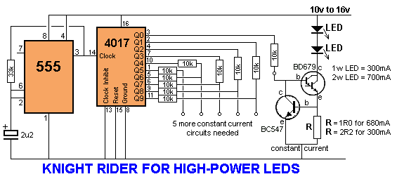
This circuit provides constant current so the LEDs are not over-driven.
KNIGHT RIDER "RUNNING HOLE" EFFECT
KNIGHT RIDER "RUNNING HOLE" EFFECT
CROSSING LIGHTS
A magnet on the train activates the TRIGGER reed switch to turn on the amber LED for a time determined by the value of the first 10u and 47k.
When the first 555 IC turns off, the 100n is uncharged because both ends are at rail voltage and it pulses pin 2 of the middle 555 LOW. This activates the 555 and pin 3 goes HIGH. This pin supplies rail voltage to the third 555 and the two red LEDs are alternately flashed. When the train passes the CANCEL reed switch, pin 4 of the middle 555 is taken LOW and the red LEDs stop flashing.
See it in action: Movie (4MB)
The circuit can also be constructed with a 40106 HEX Schmitt trigger IC (74C14). The 555 circuit consumes about 30mA when sitting and waiting. The 40106 circuit consumes less than 1mA. 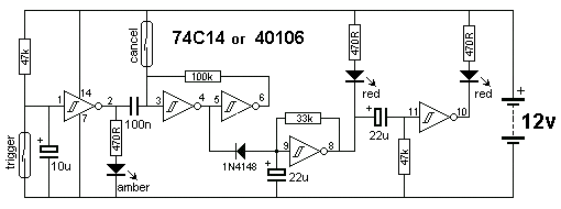
LED DICE
This circuit produces a realistic effect of the "pips" on the face of a dice. The circuit has "slow-down" to give the effect of the dice "rolling."
See the full project: LED DICE
A SIMPLER CIRCUIT:
The circuit above can be simplified and output Pin 12 can be used to illuminate two of the LEDs as this line is HIGH for the times when Q0, Q1, Q2, Q3, and Q4 are HIGH and goes LOW when Q5 - Q9 is HIGH.
This means the 4017 starts with Q0 HIGH. But Q0 is not an output. This means that when Q0 is HIGH, "carry out" is HIGH and "2" will be displayed. The next clock cycle will produce "3" on the display when Q1 is HIGH, then "4" when Q2 is HIGH, "5" when Q3 is HIGH and "6" when Q4 is HIGH. When Q5 goes HIGH, it illuminates "1" on the display because "carry out" goes LOW.
LED DICE - minimum componentsLED DICE - using CD4018 5-bit Counter X . I
ELECTRONIC SYSTEM COUNT ROLLING ( CONTROLL )
Electronic Systems
An Electronic System is a physical interconnection of components, or parts, that gathers various amounts of information together.It does this with the aid of input devices such as sensors, that respond in some way to this information and then uses electrical energy in the form of an output action to control a physical process or perform some type of mathematical operation on the signal.
But electronic control systems can also be regarded as a process that transforms one signal into another so as to give the desired system response. Then we can say that a simple electronic system consists of an input, a process, and an output with the input variable to the system and the output variable from the system both being signals.
There are many ways to represent a system, for example: mathematically, descriptively, pictorially or schematically. Electronic systems are generally represented schematically as a series of interconnected blocks and signals with each block having its own set of inputs and outputs.
As a result, even the most complex of electronic control systems can be represented by a combination of simple blocks, with each block containing or representing an individual component or complete sub-system. The representing of an electronic system or process control system as a number of interconnected blocks or boxes is known commonly as “block-diagram representation”.
Block Diagram Representation of a Simple Electronic System
In other words, an electronic system can be classed as “causal” in nature as there is a direct relationship between its input and its output. Electronic systems analysis and process control theory are generally based upon this Cause and Effect analysis.
So for example in an audio system, a microphone (input device) causes sound waves to be converted into electrical signals for the amplifier to amplify (a process), and a loudspeaker (output device) produces sound waves as an effect of being driven by the amplifiers electrical signals.
But an electronic system need not be a simple or single operation. It can also be an interconnection of several sub-systems all working together within the same overall system.
Our audio system could for example, involve the connection of a CD player, or a DVD player, an MP3 player, or a radio receiver all being multiple inputs to the same amplifier which in turn drives one or more sets of stereo or home theatre type surround loudspeakers.
But an electronic system can not just be a collection of inputs and outputs, it must “do something”, even if it is just to monitor a switch or to turn “ON” a light. We know that sensors are input devices that detect or turn real world measurements into electronic signals which can then be processed. These electrical signals can be in the form of either voltages or currents within a circuit. The opposite or output device is called an actuator, that converts the processed signal into some operation or action, usually in the form of mechanical movement.
Types of Electronic System
Electronic systems operate on either continuous-time (CT) signals or discrete-time (DT) signals. A continuous-time system is one in which the input signals are defined along a continuum of time, such as an analogue signal which “continues” over time producing a continuous-time signal.But a continuous-time signal can also vary in magnitude or be periodic in nature with a time period T. As a result, continuous-time electronic systems tend to be purely analogue systems producing a linear operation with both their input and output signals referenced over a set period of time.
Generally, most of the signals present in the physical world which we can use tend to be continuous-time signals. For example, voltage, current, temperature, pressure, velocity, etc.
On the other hand, a discrete-time system is one in which the input signals are not continuous but a sequence or a series of signal values defined in “discrete” points of time. This results in a discrete-time output generally represented as a sequence of values or numbers.
Generally a discrete signal is specified only at discrete intervals, values or equally spaced points in time. So for example, the temperature of a room measured at 1pm, at 2pm, at 3pm and again at 4pm without regards for the actual room temperature in between these points at say, 1:30pm or at 2:45pm.
Then we can represent the input and output signals of a system as x and y respectively with the signal, or signals themselves being represented by the variable, t, which usually represents time for a continuous system and the variable n, which represents an integer value for a discrete system as shown.
Continuous-time and Discrete-time System
Interconnection of Systems
One of the practical aspects of electronic systems and block-diagram representation is that they can be combined together in either a series or parallel combinations to form much bigger systems. Many larger real systems are built using the interconnection of several sub-systems and by using block diagrams to represent each subsystem, we can build a graphical representation of the whole system being analysed.When subsystems are combined to form a series circuit, the overall output at y(t) will be equivalent to the multiplication of the input signal x(t) as shown as the subsystems are
cascaded together.
Series Connected System
Then the original input signal is cascaded through a series connected system, so for two series connected subsystems, the equivalent single output will be equal to the multiplication of the systems, ie, y(t) = G1(s) x G2(s). Where G represents the transfer function of the subsystem.
Note that the term “Transfer Function” of a system refers to and is defined as being the mathematical relationship between the systems input and its output, or output/input and hence describes the behaviour of the system.
Also, for a series connected system, the order in which a series operation is performed does not matter with regards to the input and output signals as: G1(s) x G2(s) is the same as G2(s) x G1(s). An example of a simple series connected circuit could be a single microphone feeding an amplifier followed by a speaker.
Parallel Connected Electronic System
An example of a simple parallel connected circuit could be several microphones feeding into a mixing desk which in turn feeds an amplifier and speaker system.
Electronic Feedback Systems
Another important interconnection of systems which is used extensively in control systems, is the “feedback configuration”. In feedback systems, a fraction of the output signal is “fed back” and either added to or subtracted from the original input signal. The result is that the output of the system is continually altering or updating its input with the purpose of modifying the response of a system to improve stability. A feedback system is also commonly referred to as a “Closed-loop System” as shown.Closed-Loop Feedback System
An example of a simple feedback system could be a thermostatically controlled heating system in the home. If the home is too hot, the feedback loop will switch “OFF” the heating system to make it cooler. If the home is too cold, the feedback loop will switch “ON” the heating system to make it warmer. In this instance, the system comprises of the heating system, the air temperature and the thermostatically controlled feedback loop.
Transfer Function of Systems
In this case, G represents the Transfer Function of the system or subsystem. When discussing electronic systems in terms of their transfer function, the complex operator, s is used, then the equation for the gain is rewritten as: G(s) = θo(s)/θi(s)
Electronic System Summary
We have seen that a simple Electronic System consists of an input, a process, an output and possibly feedback. Electronic systems can be represented using interconnected block diagrams where the lines between each block or subsystem represents both the flow and direction of a signal through the system.Block diagrams need not represent a simple single system but can represent very complex systems made from many interconnected subsystems. These subsystems can be connected together in series, parallel or combinations of both depending upon the flow of the signals.
We have also seen that electronic signals and systems can be of continuous-time or discrete-time in nature and may be analogue, digital or both. Feedback loops can be used be used to increase or reduce the performance of a particular system by providing better stability and control. Control is the process of making a system variable adhere to a particular value, called the reference value.
Understanding And Excess Microcontroller
Microcontroller, as a breakthrough microprocessor technology and microcomputer is a new technology to meet market needs. Microcontroller as a new technology, semiconductor technology with more transistor content but requires only a small space so that microcontroller can be mass produced (in large quantities) make the price cheaper (compared to microprocessors). Microcontroller as a market need, microcontroller is present to meet the tastes of industry and consumers will the needs and desires of tools and toys even better and more sophisticated.
Unlike computer systems, capable of handling a variety of application programs (eg word processing, number processing and so on), microcontrollers can only be used for a particular application (only one program can be stored). Another difference lies in the ratio of RAM and ROM. In computer systems the ratio of RAM and ROM is large, meaning that user programs are stored in relatively large RAM space, while hardware interface routines are stored in small ROM spaces. While on the Microcontroller, the ratio of ROM and RAM is large, it means that the control program is stored in ROM (can Masked ROM or Flash PEROM) which is relatively larger, while RAM is used as a temporary storage, including the registers used in microcontroller Concerned
There are several members of microcontroller MCS51 that has internal memory, one of them is microcontroller AT89C51 which is EEPROM version of 80C51 where this internal memory can be programmed and removed electrically and produced by ATMEL Corporation. AT89C51 is made compatible with the MCS-51 standard industrial output and output cells that have 4Kbyte of internal RAM with EEPROM flash technology that can store data even when the power supply is turned off.
The MCS-51 family is an 8 bit microcontroller as shown in the following table:
Device
|
Internal memory program
|
Internal memory data
|
Timer/efen Counter
|
Interupts
|
| 8052AH 8051AH 8051 8032AH 8031AH 8031 8751H 8751H-12 8751H-88 | 8K x 8ROM 4K x 8ROM 4K x 8ROM None None None 4K x 8ROM 4K x 8ROM 4K x 8ROM | 256 x 8RAM 128 x 8RAM 128 x 8RAM 256 x 8RAM 128 x 8RAM 128 x 8RAM 128 x 8RAM 128 x 8RAM 128 x 8RAM | 3 x 16 Bit 2 x 16 Bit 2 x 16 Bit 2 x 16 Bit 2 x 16 Bit 2 x 16 Bit 2 x 16 Bit 2 x 16 Bit 2 x 16 Bit | 6 5 5 6 5 5 5 5 5 |
X . II
OPEN LOOP SYSTEM
Open-loop System
In the last tutorial about Electronic Systems, we saw that a system can be a collection of subsystems which direct or control an input signal. The function of any electronic system is to automatically regulate the output and keep it within the systems desired input value or “set point”. If the systems input changes for whatever reason, the output of the system must respond accordingly and change itself to reflect the new input value.Likewise, if something happens to disturb the systems output without any change to the input value, the output must respond by returning back to its previous set value. In the past, electrical control systems were basically manual or what is called an Open-loop System with very few automatic control or feedback features built in to regulate the process variable so as to maintain the desired output level or value.
For example, an electric clothes dryer. Depending upon the amount of clothes or how wet they are, a user or operator would set a timer (controller) to say 30 minutes and at the end of the 30 minutes the drier will automatically stop and turn-off even if the clothes are still wet or damp.
In this case, the control action is the manual operator assessing the wetness of the clothes and setting the process (the drier) accordingly.
So in this example, the clothes dryer would be an open-loop system as it does not monitor or measure the condition of the output signal, which is the dryness of the clothes. Then the accuracy of the drying process, or success of drying the clothes will depend on the experience of the user (operator).
However, the user may adjust or fine tune the drying process of the system at any time by increasing or decreasing the timing controllers drying time, if they think that the original drying process will not be met. For example, increasing the timing controller to 40 minutes to extend the drying process. Consider the following open-loop block diagram.
Open-loop Drying System
Also, an open-loop system has no knowledge of the output condition so cannot self-correct any errors it could make when the preset value drifts, even if this results in large deviations from the preset value.
Another disadvantage of open-loop systems is that they are poorly equipped to handle disturbances or changes in the conditions which may reduce its ability to complete the desired task. For example, the dryer door opens and heat is lost. The timing controller continues regardless for the full 30 minutes but the clothes are not heated or dried at the end of the drying process. This is because there is no information fed back to maintain a constant temperature.
The objective of feed forward control, also known as predictive control, is to measure or predict any potential open-loop disturbances and compensate for them manually before the controlled variable deviates too far from the original set point. So for our simple example above, if the dryers door was open it would be detected and closed allowing the drying process to continue.
Then we can define the main characteristics of an “Open-loop system” as being:
- There is no comparison between actual and desired values.
- An open-loop system has no self-regulation or control action over the output value.
- Each input setting determines a fixed operating position for the controller.
- Changes or disturbances in external conditions does not result in a direct output change.
(unless the controller setting is altered manually)
Generally, we do not have to manipulate the open-loop block diagram to calculate its actual transfer function. We can just write down the proper relationships or equations from each block diagram, and then calculate the final transfer function from these equations as shown.
Open-loop System
Open-loop control systems are often used with processes that require the sequencing of events with the aid of “ON-OFF” signals. For example a washing machines which requires the water to be switched “ON” and then when full is switched “OFF” followed by the heater element being switched “ON” to heat the water and then at a suitable temperature is switched “OFF”, and so on.
This type of “ON-OFF” open-loop control is suitable for systems where the changes in load occur slowly and the process is very slow acting, necessitating infrequent changes to the control action by an operator.
Open-loop Control Systems Summary
We have seen that a controller can manipulate its inputs to obtain the desired effect on the output of a system. One type of control system in which the output has no influence or effect on the control action of the input signal is called an Open-loop system.An “open-loop system” is defined by the fact that the output signal or condition is neither measured nor “fed back” for comparison with the input signal or system set point. Therefore open-loop systems are commonly referred to as “Non-feedback systems”.
Also, as an open-loop system does not use feedback to determine if its required output was achieved, it “assumes” that the desired goal of the input was successful because it cannot correct any errors it could make, and so cannot compensate for any external disturbances to the system.
Open-loop Motor Control
So for example, assume the DC motor controller as shown. The speed of rotation of the motor will depend upon the voltage supplied to the amplifier (the controller) by the potentiometer. The value of the input voltage could be proportional to the position of the potentiometer.Then the position of the potentiometers slider represents the input, θi which is amplified by the amplifier (controller) to drive the DC motor (process) at a set speed N representing the output, θo of the system. The motor will continue to rotate at a fixed speed determined by the position of the potentiometer.
As the signal path from the input to the output is a direct path not forming part of any loop, the overall gain of the system will the cascaded values of the individual gains from the potentiometer, amplifier, motor and load. It is clearly desirable that the output speed of the motor should be identical to the position of the potentiometer, giving the overall gain of the system as unity.
However, the individual gains of the potentiometer, amplifier and motor may vary over time with changes in supply voltage or temperature, or the motors load may increase representing external disturbances to the open-loop motor control system.
But the user will eventually become aware of the change in the systems performance (change in motor speed) and may correct it by increasing or decreasing the potentiometers input signal accordingly to maintain the original or desired speed.
The advantages of this type of “open-loop motor control” is that it is potentially cheap and simple to implement making it ideal for use in well-defined systems were the relationship between input and output is direct and not influenced by any outside disturbances. Unfortunately this type of open-loop system is inadequate as variations or disturbances in the system affect the speed of the motor. Then another form of control is required.
X . III
CLOSED LOOP SYSTEM
Closed-loop Systems
Systems in which the output quantity has no effect upon the input to the control process are called open-loop control systems, and that open-loop systems are just that, open ended non-feedback systems.But the goal of any electrical or electronic control system is to measure, monitor, and control a process and one way in which we can accurately control the process is by monitoring its output and “feeding” some of it back to compare the actual output with the desired output so as to reduce the error and if disturbed, bring the output of the system back to the original or desired response.
The quantity of the output being measured is called the “feedback signal”, and the type of control system which uses feedback signals to both control and adjust itself is called a Close-loop System.
A Closed-loop Control System, also known as a feedback control system is a control system which uses the concept of an open loop system as its forward path but has one or more feedback loops (hence its name) or paths between its output and its input. The reference to “feedback”, simply means that some portion of the output is returned “back” to the input to form part of the systems excitation.
Closed-loop systems are designed to automatically achieve and maintain the desired output condition by comparing it with the actual condition. It does this by generating an error signal which is the difference between the output and the reference input. In other words, a “closed-loop system” is a fully automatic control system in which its control action being dependent on the output in some way.
So for example, consider our electric clothes dryer from the previous open-loop tutorial. Suppose we used a sensor or transducer (input device) to continually monitor the temperature or dryness of the clothes and feed a signal relating to the dryness back to the controller as shown below.
Closed-loop Control
Then the closed-loop configuration is characterised by the feedback signal, derived from the sensor in our clothes drying system. The magnitude and polarity of the resulting error signal, would be directly related to the difference between the required dryness and actual dryness of the clothes.
Also, because a closed-loop system has some knowledge of the output condition, (via the sensor) it is better equipped to handle any system disturbances or changes in the conditions which may reduce its ability to complete the desired task.
For example, as before, the dryer door opens and heat is lost. This time the deviation in temperature is detected by the feedback sensor and the controller self-corrects the error to maintain a constant temperature within the limits of the preset value. Or possibly stops the process and activates an alarm to inform the operator.
As we can see, in a closed-loop control system the error signal, which is the difference between the input signal and the feedback signal (which may be the output signal itself or a function of the output signal), is fed to the controller so as to reduce the systems error and bring the output of the system back to a desired value. In our case the dryness of the clothes. Clearly, when the error is zero the clothes are dry.
The term Closed-loop control always implies the use of a feedback control action in order to reduce any errors within the system, and its “feedback” which distinguishes the main differences between an open-loop and a closed-loop system.The accuracy of the output thus depends on the feedback path, which in general can be made very accurate and within electronic control systems and circuits, feedback control is more commonly used than open-loop or feed forward control.
Closed-loop systems have many advantages over open-loop systems. The primary advantage of a closed-loop feedback control system is its ability to reduce a system’s sensitivity to external disturbances, for example opening of the dryer door, giving the system a more robust control as any changes in the feedback signal will result in compensation by the controller.
Then we can define the main characteristics of Closed-loop Control as being:
- To reduce errors by automatically adjusting the systems input.
- To improve stability of an unstable system.
- To increase or reduce the systems sensitivity.
- To enhance robustness against external disturbances to the process.
- To produce a reliable and repeatable performance.
Closed-loop Summing Points
For a closed-loop feedback system to regulate any control signal, it must first determine the error between the actual output and the desired output. This is achieved using a summing point, also referred to as a comparison element, between the feedback loop and the systems input. These summing points compare a systems set point to the actual value and produce a positive or negative error signal which the controller responds too. where: Error = Set point – Actual CROSS A NEW TESTAMENT PID / PITa memory flyer Summing Point Types
Closed-loop System Transfer Function
The Transfer Function of any electrical or electronic control system is the mathematical relationship between the systems input and its output, and hence describes the behaviour of the system. Note also that the ratio of the output of a particular device to its input represents its gain. Then we can correctly say that the output is always the transfer function of the system times the input. Consider the closed-loop system below.Typical Closed-loop System Representation
To find the transfer function of the closed-loop system above, we must first calculate the output signal θo in terms of the input signal θi. To do so, we can easily write the equations of the given block-diagram as follows.
The output from the system is equal to: Output = G x Error
Note that the error signal, θe is also the input to the feed-forward block: G
The output from the summing point is equal to: Error = Input - H x Output
If H = 1 (unity feedback) then:
The output from the summing point will be: Error (θe) = Input - Output
Eliminating the error term, then:
The output is equal to: Output = G x (Input - H x Output)
Therefore: G x Input = Output + G x H x Output
Rearranging the above gives us the closed-loop transfer function of:
We can see that when H = 1 (unity feedback) and G is very large, the transfer function approaches unity as:
Multi-loop Closed-loop System
Whilst our example above is of a single input, single output closed-loop system, the basic transfer function still applies to more complex multi-loop systems. Most practical feedback circuits have some form of multiple loop control, and for a multi-loop configuration the transfer function between a controlled and a manipulated variable depends on whether the other feedback control loops are open or closed.Consider the multi-loop system below.
Closed-loop Motor Control
So how can we use Closed-loop Systems in Electronics. Well consider our DC motor controller from the previous open-loop tutorial. If we connected a speed measuring transducer, such as a tachometer to the shaft of the DC motor, we could detect its speed and send a signal proportional to the motor speed back to the amplifier. A tachometer, also known as a tacho-generator is simply a permanent-magnet DC generator which gives a DC output voltage proportional to the speed of the motor.Then the position of the potentiometers slider represents the input, θi which is amplified by the amplifier (controller) to drive the DC motor at a set speed N representing the output, θo of the system, and the tachometer T would be the closed-loop back to the controller. The difference between the input voltage setting and the feedback voltage level gives the error signal as shown.
Closed-loop Motor Control
This difference would produce an error signal which the controller would automatically respond too adjusting the motors speed. Then the controller works to minimize the error signal, with zero error indicating actual speed which equals set point.
Electronically, we could implement such a simple closed-loop tachometer-feedback motor control circuit using an operational amplifier (op-amp) for the controller as shown.
Closed-loop Motor Controller Circuit
Block Diagram for the Feedback Controller
Closed-loop Systems Summary
We have seen that an electronic control system with one or more feedback paths is called a Closed-loop System. Closed-loop control systems are also called “feedback control systems” are very common in process control and electronic control systems. Feedback systems have part of their output signal “fed back” to the input for comparison with the desired set point condition. The type of feedback signal can result either in positive feedback or negative feedback.In a closed-loop system, a controller is used to compare the output of a system with the required condition and convert the error into a control action designed to reduce the error and bring the output of the system back to the desired response. Then closed-loop control systems use feedback to determine the actual input to the system and can have more than one feedback loop.
Closed-loop control systems have many advantages over open-loop systems. One advantage is the fact that the use of feedback makes the system response relatively insensitive to external disturbances and internal variations in system parameters such as temperature. It is thus possible to use relatively inaccurate and inexpensive components to obtain the accurate control of a given process or plant.
However, system stability can be a major problem especially in badly designed closed-loop systems as they may try to over-correct any errors which could cause the system to loss control and oscillate.
In the next tutorial about Electronics Systems, we will look at the different ways in which we can incorporate a summing point into the input of a system and the different ways in which we can feed signals back to it.
X . IIII
FEEDBACK SYSTEM
Feedback Systems
Feedback Systems process signals and as such are signal processors. The processing part of a feedback system may be electrical or electronic, ranging from a very simple to a highly complex circuits.Simple analogue feedback control circuits can be constructed using individual or discrete components, such as transistors, resistors and capacitors, etc, or by using microprocessor-based and integrated circuits (IC’s) to form more complex digital feedback systems.
As we have seen, open-loop systems are just that, open ended, and no attempt is made to compensate for changes in circuit conditions or changes in load conditions due to variations in circuit parameters, such as gain and stability, temperature, supply voltage variations and/or external disturbances. But the effects of these “open-loop” variations can be eliminated or at least considerably reduced by the introduction of Feedback.
A feedback system is one in which the output signal is sampled and then fed back to the input to form an error signal that drives the system. In the previous tutorial about Closed-loop Systems, we saw that in general, feedback is comprised of a sub-circuit that allows a fraction of the output signal from a system to modify the effective input signal in such a way as to produce a response that can differ substantially from the response produced in the absence of such feedback.
Feedback Systems are very useful and widely used in amplifier circuits, oscillators, process control systems as well as other types of electronic systems. But for feedback to be an effective tool it must be controlled as an uncontrolled system will either oscillate or fail to function. The basic model of a feedback system is given as:
Feedback System Block Diagram Model
- Circuit characteristics such as the systems gain and response can be precisely controlled.
- Circuit characteristics can be made independent of operating conditions such as supply voltages or temperature variations.
- Signal distortion due to the non-linear nature of the components used can be greatly reduced.
- The Frequency Response, Gain and Bandwidth of a circuit or system can be easily controlled to within tight limits.
Positive Feedback Systems
In a “positive feedback control system”, the set point and output values are added together by the controller as the feedback is “in-phase” with the input. The effect of positive (or regenerative) feedback is to “increase” the systems gain, ie, the overall gain with positive feedback applied will be greater than the gain without feedback. For example, if someone praises you or gives you positive feedback about something, you feel happy about yourself and are full of energy, you feel more positive.However, in electronic and control systems to much praise and positive feedback can increase the systems gain far too much which would give rise to oscillatory circuit responses as it increases the magnitude of the effective input signal.
An example of a positive feedback systems could be an electronic amplifier based on an operational amplifier, or op-amp as shown.
Positive Feedback System
If the input voltage Vin is positive, the op-amp amplifies this positive signal and the output becomes more positive. Some of this output voltage is returned back to the input by the feedback network.
Thus the input voltage becomes more positive, causing an even larger output voltage and so on. Eventually the output becomes saturated at its positive supply rail.
Likewise, if the input voltage Vin is negative, the reverse happens and the op-amp saturates at its negative supply rail. Then we can see that positive feedback does not allow the circuit to function as an amplifier as the output voltage quickly saturates to one supply rail or the other, because with positive feedback loops “more leads to more” and “less leads to less”.
Then if the loop gain is positive for any system the transfer function will be: Av = G / (1 – GH). Note that if GH = 1 the system gain Av = infinity and the circuit will start to self-oscillate, after which no input signal is needed to maintain oscillations, which is useful if you want to make an oscillator.
Although often considered undesirable, this behaviour is used in electronics to obtain a very fast switching response to a condition or signal. One example of the use of positive feedback is hysteresis in which a logic device or system maintains a given state until some input crosses a preset threshold. This type of behaviour is called “bi-stability” and is often associated with logic gates and digital switching devices such as multivibrators.
We have seen that positive or regenerative feedback increases the gain and the possibility of instability in a system which may lead to self-oscillation and as such, positive feedback is widely used in oscillatory circuits such as Oscillators and Timing circuits.
Negative Feedback Systems
In a “negative feedback control system”, the set point and output values are subtracted from each other as the feedback is “out-of-phase” with the original input. The effect of negative (or degenerative) feedback is to “reduce” the gain. For example, if someone criticises you or gives you negative feedback about something, you feel unhappy about yourself and therefore lack energy, you feel less positive.Because negative feedback produces stable circuit responses, improves stability and increases the operating bandwidth of a given system, the majority of all control and feedback systems is degenerative reducing the effects of the gain.
An example of a negative feedback system is an electronic amplifier based on an operational amplifier as shown.
Negative Feedback System
If the input voltage Vin is positive, the op-amp amplifies this positive signal, but because its connected to the inverting input of the amplifier, and the output becomes more negative. Some of this output voltage is returned back to the input by the feedback network of Rf.
Thus the input voltage is reduced by the negative feedback signal, causing an even smaller output voltage and so on. Eventually the output will settle down and become stabilised at a value determined by the gain ratio of Rf ÷ Rin.
Likewise, if the input voltage Vin is negative, the reverse happens and the op-amps output becomes positive (inverted) which adds to the negative input signal. Then we can see that negative feedback allows the circuit to function as an amplifier, so long as the output is within the saturation limits.
So we can see that the output voltage is stabilised and controlled by the feedback, because with negative feedback loops “more leads to less” and “less leads to more”.
Then if the loop gain is positive for any system the transfer function will be: Av = G / (1 + GH).
The use of negative feedback in amplifier and process control systems is widespread because as a rule negative feedback systems are more stable than positive feedback systems, and a negative feedback system is said to be stable if it does not oscillate by itself at any frequency except for a given circuit condition.
Another advantage is that negative feedback also makes control systems more immune to random variations in component values and inputs. Of course nothing is for free, so it must be used with caution as negative feedback significantly modifies the operating characteristics of a given system.
Classification of Feedback Systems
Thus far we have seen the way in which the output signal is “fed back” to the input terminal, and for feedback systems this can be of either, Positive Feedback or Negative Feedback. But the manner in which the output signal is measured and introduced into the input circuit can be very different leading to four basic classifications of feedback.Based on the input quantity being amplified, and on the desired output condition, the input and output variables can be modelled as either a voltage or a current. As a result, there are four basic classifications of single-loop feedback system in which the output signal is fed back to the input and these are:
- Series-Shunt Configuration – Voltage in and Voltage out or Voltage Controlled Voltage Source (VCVS).
- Shunt-Shunt Configuration – Current in and Voltage out or Current Controlled Voltage Source (CCVS).
- Series-Series Configuration – Voltage in and Current out or Voltage Controlled Current Source (VCCS).
- Shunt-Series Configuration – Current in and Current out or Current Controlled Current Source (CCCS).
Series-Shunt Feedback Systems
Series-Shunt Feedback, also known as series voltage feedback, operates as a voltage-voltage controlled feedback system. The error voltage fed back from the feedback network is in series with the input. The voltage which is fed back from the output being proportional to the output voltage, Vo as it is parallel, or shunt connected.Series-Shunt Feedback System
Then the “series-shunt feedback configuration” works as a true voltage amplifier as the input signal is a voltage and the output signal is a voltage, so the transfer gain is given as: Av = Vout ÷ Vin. Note that this quantity is dimensionless as its units are volts/volts.
Shunt-Series Feedback Systems
Shunt-Series Feedback, also known as shunt current feedback, operates as a current-current controlled feedback system. The feedback signal is proportional to the output current, Io flowing in the load. The feedback signal is fed back in parallel or shunt with the input as shown.Shunt-Series Feedback System
This parallel shunt feedback connection will not normally affect the voltage gain of the system, since for a voltage output a voltage input is required. Also, the series connection at the output increases output resistance, Rout while the shunt connection at the input decreases the input resistance, Rin.
Then the “shunt-series feedback configuration” works as a true current amplifier as the input signal is a current and the output signal is a current, so the transfer gain is given as: Ai = Iout ÷ Iin. Note that this quantity is dimensionless as its units are amperes/amperes.
Series-Series Feedback Systems
Series-Series Feedback Systems, also known as series current feedback, operates as a voltage-current controlled feedback system. In the series current configuration the feedback error signal is in series with the input and is proportional to the load current, Iout. Actually, this type of feedback converts the current signal into a voltage which is actually fed back and it is this voltage which is subtracted from the input.Series-Series Feedback System
Then the “series-series feedback configuration” functions as transconductance type amplifier system as the input signal is a voltage and the output signal is a current. then for a series-series feedback circuit the transfer gain is given as: Gm = Iout ÷ Vin.
Shunt-Shunt Feedback Systems
Shunt-Shunt Feedback Systems, also known as shunt voltage feedback, operates as a current-voltage controlled feedback system. In the shunt-shunt feedback configuration the signal fed back is in parallel with the input signal. The output voltage is sensed and the current is subtracted from the input current in shunt, and as such its the currents, not the voltages that subtract.Shunt-Shunt Feedback System
Then the shunt voltage configuration works as transresistance type voltage amplifier as the input signal is a current and the output signal is a voltage, so the transfer gain is given as: Rm = Vout ÷ Iin.
Feedback Systems Summary
We have seen that a Feedback System is one in which the output signal is sampled and then fed back to the input to form an error signal that drives the system, and depending on the type of feedback used, the feedback signal which is mixed with the systems input signal, can be either a voltage or a current.Feedback will always change the performance of a system and feedback arrangements can be either positive (regenerative) or negative (degenerative) type feedback systems. If the feedback loop around the system produces a loop-gain which is negative, the feedback is said to be negative or degenerative with the main effect of the negative feedback is in reducing the systems gain.
If however the gain around the loop is positive, the system is said to have positive feedback or regenerative feedback. The effect of positive feedback is to increase the gain which can cause a system to become unstable and oscillate especially if GH = -1.
We have also seen that block-diagrams can be used to demonstrate the various types of feedback systems. In the block diagrams above, the input and output variables can be modelled as either a voltage or a current and as such there are four combinations of inputs and outputs that represent the possible types of feedback, namely: Series Voltage Feedback, Shunt Voltage Feedback, Series Current Feedback and Shunt Current Feedback.
The names for these different types of feedback systems are derived from the way that the feedback network connects between the input and output stages either in parallel (shunt) or series.
In the next THEME about Feedback Systems, we will look at the effects of Negative Feedback on a system and see how it can be used to improve a control systems stability.
X . IIIII
Negative Feedback Systems
Negative Feedback Systems
Negative Feedback, NFB is the most common form of feedback control used in process, micro-computer and amplifier systems.Feedback is the process by which a fraction of the output signal, either a voltage or a current, is used as an input. If this feed back fraction is opposite in value or phase (“anti-phase”) to the input signal, then the feedback is said to be Negative Feedback, or degenerative feedback.
Negative feedback opposes or subtracts from the input signals giving it many advantages in the design and stabilisation of control systems. For example, if the systems output changes for any reason, then negative feedback affects the input in such a way as to counteract the change.
Feedback reduces the overall gain of a system with the degree of reduction being related to the systems open-loop gain. Negative feedback also has effects of reducing distortion, noise, sensitivity to external changes as well as improving system bandwidth and input and output impedances.
Feedback in an electronic system, whether negative feedback or positive feedback is unilateral in direction. Meaning that its signals flow one way only from the output to the input of the system. This then makes the loop gain, G of the system independent of the load and source impedances.
As feedback implies a closed-loop system it must therefore have a summing point. In a negative feedback system this summing point or junction at its input subtracts the feedback signal from the input signal to form an error signal, β which drives the system. If the system has a positive gain, the feedback signal must be subtracted from the input signal in order for the feedback to be negative as shown.
Negative Feedback Circuit
Then using the basic closed-loop circuit above we can derive the general feedback equation as being:
Negative Feedback Equation
Effects of Negative Feedback
If the open-loop gain, G is very large, then βG will be much greater than 1, so that the overall gain of the system is roughly equal to 1/β. If the open-loop gain decreases due to frequency or the effects of system ageing, providing that βG is still relatively large, the overall system gain does not change very much. So negative feedback tends to reduce the effects of gain change giving what is generally called “gain stability”.Negative Feedback Example No1
A system has a gain of 80dB without feedback. If the negative feedback fraction is 1/50th. Calculate the closed-loop gain of the system in dB with the addition of negative feedback.Negative Feedback Example No2
If after 5 years the loop gain of the system without negative feedback has fallen to 60dB and the feedback fraction has remained constant at 1/50th. Calculate the new closed-loop gain value of the system.However with the addition of negative feedback the systems gain has only fallen from 34dB to 33.5dB, a reduction of less than 1.5%, which proves that negative feedback gives added stability to a systems gain.
Therefore we can see that by applying negative feedback to a system greatly reduces its overall gain compared to its gain without feedback.
The systems gain without feedback can be very large but not precise as it may change from one system device to the next, then it is possible to design a system with sufficient open-loop gain that, after the negative feedback has been added, the overall gain matches the desired value.
Also, if the feedback network is constructed from passive elements having stable characteristics, the overall gain becomes very steady and unaffected by variation in the systems inherent open-loop gain.
Negative Feedback in Operational Amplifiers
Operational amplifiers (op-amps) are the most commonly used type of linear integrated circuit but they have a very high gain. The open-loop voltage gain, AVOL, of a standard 741 op-amp is its voltage gain when there is no negative feedback applied and the open-loop voltage gain of an op-amp is the ratio of its output voltage, Vout, to its differential input voltage, Vin, ( Vout/Vin ).The typical value of AVOL for a 741 op-amp is more than 200,000 (106dB). So an input voltage signal of only 1mV, would result in an output voltage of over 200 volts! forcing the output immediately into saturation. Obviously this high open-loop voltage gain needs to be controlled in some way, and we can do just that by using negative feedback.
The use of negative feedback can significantly improve the performance of an operational amplifier and any op-amp circuit that does not use negative feedback is considered too unstable to be useful. But how can we use negative feedback to control an op-amp. Well consider the circuit below of a Non-inverting Operational Amplifier.
Non-inverting Op-amp Circuit
Negative Feedback Example No3
An operational amplifier with an open-loop voltage gain, AVOL of 320,000 without feedback is to be used as a non-inverting amplifier. Calculate the values of the feedback resistances, R1 and R2 required to stabilise the circuit with a closed loop gain of 20.The generalised closed-loop feedback equation we derived above is given as:
As the resistors, R1 and R2 form a simple series-voltage potential divider network across the non-inverting amplifier, the closed-loop voltage gain of the circuit will be determined by the ratios of these resistances as:
Non-inverting Op-amp Circuit
X . IIIIII
energy transfer to Transformer Basics
Transformer Basics
Transformer Basics
One of the main reasons that we use alternating AC voltages and currents in our homes and workplace’s is that AC supplies can be easily generated at a convenient voltage, transformed (hence the name transformer) into much higher voltages and then distributed around the country using a national grid of pylons and cables over very long distances.The reason for transforming the voltage to a much higher level is that higher distribution voltages implies lower currents for the same power and therefore lower I2R losses along the networked grid of cables. These higher AC transmission voltages and currents can then be reduced to a much lower, safer and usable voltage level where it can be used to supply electrical equipment in our homes and workplaces, and all this is possible thanks to the basic Voltage Transformer.
A Typical Voltage Transformer
The transformer does this by linking together two or more electrical circuits using a common oscillating magnetic circuit which is produced by the transformer itself. A transformer operates on the principals of “electromagnetic induction”, in the form of Mutual Induction.
Mutual induction is the process by which a coil of wire magnetically induces a voltage into another coil located in close proximity to it. Then we can say that transformers work in the “magnetic domain”, and transformers get their name from the fact that they “transform” one voltage or current level into another.
Transformers are capable of either increasing or decreasing the voltage and current levels of their supply, without modifying its frequency, or the amount of electrical power being transferred from one winding to another via the magnetic circuit.
A single phase voltage transformer basically consists of two electrical coils of wire, one called the “Primary Winding” and another called the “Secondary Winding”. For this tutorial we will define the “primary” side of the transformer as the side that usually takes power, and the “secondary” as the side that usually delivers power. In a single-phase voltage transformer the primary is usually the side with the higher voltage.
These two coils are not in electrical contact with each other but are instead wrapped together around a common closed magnetic iron circuit called the “core”. This soft iron core is not solid but made up of individual laminations connected together to help reduce the core’s losses.
The two coil windings are electrically isolated from each other but are magnetically linked through the common core allowing electrical power to be transferred from one coil to the other. When an electric current passed through the primary winding, a magnetic field is developed which induces a voltage into the secondary winding as shown.
Single Phase Voltage Transformer
Transformer Construction (single-phase)
- Where:
- VP - is the Primary Voltage
- VS - is the Secondary Voltage
- NP - is the Number of Primary Windings
- NS - is the Number of Secondary Windings
- Φ (phi) - is the Flux Linkage
However, a third condition exists in which a transformer produces the same voltage on its secondary as is applied to its primary winding. In other words, its output is identical with respect to voltage, current and power transferred. This type of transformer is called an “Impedance Transformer” and is mainly used for impedance matching or the isolation of adjoining electrical circuits.
The difference in voltage between the primary and the secondary windings is achieved by changing the number of coil turns in the primary winding ( NP ) compared to the number of coil turns on the secondary winding ( NS ).
As the transformer is basically a linear device, a ratio now exists between the number of turns of the primary coil divided by the number of turns of the secondary coil. This ratio, called the ratio of transformation, more commonly known as a transformers “turns ratio”, ( TR ). This turns ratio value dictates the operation of the transformer and the corresponding voltage available on the secondary winding.
It is necessary to know the ratio of the number of turns of wire on the primary winding compared to the secondary winding. The turns ratio, which has no units, compares the two windings in order and is written with a colon, such as 3:1 (3-to-1). This means in this example, that if there are 3 volts on the primary winding there will be 1 volt on the secondary winding, 3 volts-to-1 volt. Then we can see that if the ratio between the number of turns changes the resulting voltages must also change by the same ratio, and this is true.
Transformers are all about “ratios”. The ratio of the primary to the secondary, the ratio of the input to the output, and the turns ratio of any given transformer will be the same as its voltage ratio. In other words for a transformer: “turns ratio = voltage ratio”. The actual number of turns of wire on any winding is generally not important, just the turns ratio and this relationship is given as:
A Transformers Turns Ratio
Note that the order of the numbers when expressing a transformers turns ratio value is very important as the turns ratio 3:1 expresses a very different transformer relationship and output voltage than one in which the turns ratio is given as: 1:3.
Transformer Basics Example No1
A voltage transformer has 1500 turns of wire on its primary coil and 500 turns of wire for its secondary coil. What will be the turns ratio (TR) of the transformer.Transformer Basics Example No2
If 240 volts rms is applied to the primary winding of the same transformer above, what will be the resulting secondary no load voltage.Then the main purpose of a transformer is to transform voltages at preset ratios and we can see that the primary winding has a set amount or number of windings (coils of wire) on it to suit the input voltage. If the secondary output voltage is to be the same value as the input voltage on the primary winding, then the same number of coil turns must be wound onto the secondary core as there are on the primary core giving an even turns ratio of 1:1 (1-to-1). In other words, one coil turn on the secondary to one coil turn on the primary.
If the output secondary voltage is to be greater or higher than the input voltage, (step-up transformer) then there must be more turns on the secondary giving a turns ratio of 1:N (1-to-N), where N represents the turns ratio number. Likewise, if it is required that the secondary voltage is to be lower or less than the primary, (step-down transformer) then the number of secondary windings must be less giving a turns ratio of N:1 (N-to-1).
Transformer Action
We have seen that the number of coil turns on the secondary winding compared to the primary winding, the turns ratio, affects the amount of voltage available from the secondary coil. But if the two windings are electrically isolated from each other, how is this secondary voltage produced?We have said previously that a transformer basically consists of two coils wound around a common soft iron core. When an alternating voltage ( VP ) is applied to the primary coil, current flows through the coil which in turn sets up a magnetic field around itself, called mutual inductance, by this current flow according to Faraday’s Law of electromagnetic induction. The strength of the magnetic field builds up as the current flow rises from zero to its maximum value which is given as dΦ/dt.
However, the strength of the magnetic field induced into the soft iron core depends upon the amount of current and the number of turns in the winding. When current is reduced, the magnetic field strength reduces.
When the magnetic lines of flux flow around the core, they pass through the turns of the secondary winding, causing a voltage to be induced into the secondary coil. The amount of voltage induced will be determined by: N.dΦ/dt (Faraday’s Law), where N is the number of coil turns. Also this induced voltage has the same frequency as the primary winding voltage.
Then we can see that the same voltage is induced in each coil turn of both windings because the same magnetic flux links the turns of both the windings together. As a result, the total induced voltage in each winding is directly proportional to the number of turns in that winding. However, the peak amplitude of the output voltage available on the secondary winding will be reduced if the magnetic losses of the core are high.
If we want the primary coil to produce a stronger magnetic field to overcome the cores magnetic losses, we can either send a larger current through the coil, or keep the same current flowing, and instead increase the number of coil turns ( NP ) of the winding. The product of amperes times turns is called the “ampere-turns”, which determines the magnetising force of the coil.
So assuming we have a transformer with a single turn in the primary, and only one turn in the secondary. If one volt is applied to the one turn of the primary coil, assuming no losses, enough current must flow and enough magnetic flux generated to induce one volt in the single turn of the secondary. That is, each winding supports the same number of volts per turn.
As the magnetic flux varies sinusoidally, Φ = Φmax sinωt, then the basic relationship between induced emf, ( E ) in a coil winding of N turns is given by:
emf = turns x rate of change
- Where:
- ƒ - is the flux frequency in Hertz, = ω/2π
- Ν - is the number of coil windings.
- Φ - is the flux density in webers
Also please note that as transformers require an alternating magnetic flux to operate correctly, transformers cannot therefore be used to transform or supply DC voltages or currents, since the magnetic field must be changing to induce a voltage in the secondary winding. In other words, transformers DO NOT operate on steady state DC voltages, only alternating or pulsating voltages.
If a transformers primary winding was connected to a DC supply, the inductive reactance of the winding would be zero as DC has no frequency, so the effective impedance of the winding will therefore be very low and equal only to the resistance of the copper used. Thus the winding will draw a very high current from the DC supply causing it to overheat and eventually burn out, because as we know I = V/R.
Transformer Basics Example No3
A single phase transformer has 480 turns on the primary winding and 90 turns on the secondary winding. The maximum value of the magnetic flux density is 1.1T when 2200 volts, 50Hz is applied to the transformer primary winding. Calculate:a). The maximum flux in the core.
Electrical Power in a Transformer
Another one of the transformer basics parameters is its power rating. The power rating of a transformer is obtained by simply multiplying the current by the voltage to obtain a rating in Volt-amperes, ( VA ). Small single phase transformers may be rated in volt-amperes only, but much larger power transformers are rated in units of Kilo volt-amperes, ( kVA ) where 1 kilo volt-ampere is equal to 1,000 volt-amperes, and units of Mega volt-amperes, ( MVA ) where 1 mega volt-ampere is equal to 1 million volt-amperes.In an ideal transformer (ignoring any losses), the power available in the secondary winding will be the same as the power in the primary winding, they are constant wattage devices and do not change the power only the voltage to current ratio. Thus, in an ideal transformer the Power Ratio is equal to one (unity) as the voltage, V multiplied by the current, I will remain constant.
That is the electric power at one voltage/current level on the primary is “transformed” into electric power, at the same frequency, to the same voltage/current level on the secondary side. Although the transformer can step-up (or step-down) voltage, it cannot step-up power. Thus, when a transformer steps-up a voltage, it steps-down the current and vice-versa, so that the output power is always at the same value as the input power. Then we can say that primary power equals secondary power, ( PP = PS ).
Power in a Transformer
Note that since power loss is proportional to the square of the current being transmitted, that is: I2R, increasing the voltage, let’s say doubling ( ×2 ) the voltage would decrease the current by the same amount, ( ÷2 ) while delivering the same amount of power to the load and therefore reducing losses by factor of 4. If the voltage was increased by a factor of 10, the current would decrease by the same factor reducing overall losses by factor of 100.
Transformer Basics – Efficiency
A transformer does not require any moving parts to transfer energy. This means that there are no friction or windage losses associated with other electrical machines. However, transformers do suffer from other types of losses called “copper losses” and “iron losses” but generally these are quite small.Copper losses, also known as I2R loss is the electrical power which is lost in heat as a result of circulating the currents around the transformers copper windings, hence the name. Copper losses represents the greatest loss in the operation of a transformer. The actual watts of power lost can be determined (in each winding) by squaring the amperes and multiplying by the resistance in ohms of the winding (I2R).
Iron losses, also known as hysteresis is the lagging of the magnetic molecules within the core, in response to the alternating magnetic flux. This lagging (or out-of-phase) condition is due to the fact that it requires power to reverse magnetic molecules; they do not reverse until the flux has attained sufficient force to reverse them.
Their reversal results in friction, and friction produces heat in the core which is a form of power loss. Hysteresis within the transformer can be reduced by making the core from special steel alloys.
The intensity of power loss in a transformer determines its efficiency. The efficiency of a transformer is reflected in power (wattage) loss between the primary (input) and secondary (output) windings. Then the resulting efficiency of a transformer is equal to the ratio of the power output of the secondary winding, PS to the power input of the primary winding, PP and is therefore high.
An ideal transformer is 100% efficient because it delivers all the energy it receives. Real transformers on the other hand are not 100% efficient and at full load, the efficiency of a transformer is between 94% to 96% which is quiet good. For a transformer operating with a constant voltage and frequency with a very high capacity, the efficiency may be as high as 98%. The efficiency, η of a transformer is given as:
Transformer Efficiency
where: Input, Output and Losses are all expressed in units of power.
Generally when dealing with transformers, the primary watts are called “volt-amps”, VA to differentiate them from the secondary watts. Then the efficiency equation above can be modified to:Transformer Efficiency Triangle
Transformer Basics Summary
Then to summarise this transformer basics tutorial. A Transformer changes the voltage level (or current level) on its input winding to another value on its output winding using a magnetic field. A transformer consists of two electrically isolated coils and operates on Faraday’s principal of “mutual induction”, in which an EMF is induced in the transformers secondary coil by the magnetic flux generated by the voltages and currents flowing in the primary coil winding.Both the primary and secondary coil windings are wrapped around a common soft iron core made of individual laminations to reduce eddy current and power losses. The primary winding of the transformer is connected to the AC power source which must be sinusoidal in nature, while the secondary winding supplies power to the load.
We can represent the transformer in block diagram form as follows:
Basic Representation of the Transformer
If this ratio is less than unity, n < 1 then NS is greater than NP and the transformer is classed as a step-up transformer. If this ratio is greater than unity, n > 1, that is NP is greater than NS, the transformer is classed as a step-down transformer. Note that single phase step-down transformer can also be used as a step-up transformer simply by reversing its connections and making the low voltage winding its primary, and vice versa as long as the transformer is operated within its original VA design rating.
If the turns ratio is equal to unity, n = 1 then both the primary and secondary have the same number of windings, therefore the voltages and currents are the same for both windings.
This type of transformer is classed as an isolation transformer as both the primary and secondary windings of the transformer have the same number of volts per turn. The efficiency of a transformer is the ratio of the power it delivers to the load to the power it absorbs from the supply. In an ideal transformer there are no losses so no loss of power then Pin = Pout.
X . IIIIIII
Transformer Construction
Transformer Construction
The construction of a simple two-winding transformer consists of each winding being wound on a separate limb or core of the soft iron form which provides the necessary magnetic circuit.
This magnetic circuit, know more commonly as the “transformer core” is designed to provide a path for the magnetic field to flow around, which is necessary for induction of the voltage between the two windings.
However, this type of transformer construction were the two windings are wound on separate limbs is not very efficient since the primary and secondary windings are well separated from each other. This results in a low magnetic coupling between the two windings as well as large amounts of magnetic flux leakage from the transformer itself. But as well as this “O” shapes construction, there are different types of “transformer construction” and designs available which are used to overcome these inefficiencies producing a smaller more compact transformer.
The efficiency of a simple transformer construction can be improved by bringing the two windings within close contact with each other thereby improving the magnetic coupling. Increasing and concentrating the magnetic circuit around the coils may improve the magnetic coupling between the two windings, but it also has the effect of increasing the magnetic losses of the transformer core.
As well as providing a low reluctance path for the magnetic field, the core is designed to prevent circulating electric currents within the iron core itself. Circulating currents, called “eddy currents”, cause heating and energy losses within the core decreasing the transformers efficiency.
These losses are due mainly to voltages induced in the iron circuit, which is constantly being subjected to the alternating magnetic fields setup by the external sinusoidal supply voltage. One way to reduce these unwanted power losses is to construct the transformer core from thin steel laminations.
In all types of transformer construction, the central iron core is constructed from of a highly permeable material made from thin silicon steel laminations assembled together to provide the required magnetic path with the minimum of losses. The resistivity of the steel sheet itself is high reducing the eddy current losses by making the laminations very thin.
These steel transformer laminations vary in thickness’s from between 0.25mm to 0.5mm and as steel is a conductor, the laminations are electrically insulated from each other by a very thin coating of insulating varnish or by the use of an oxide layer on the surface.
Transformer Construction of the Core
Generally, the name associated with the construction of a transformer is dependant upon how the primary and secondary windings are wound around the central laminated steel core. The two most common and basic designs of transformer construction are the Closed-core Transformer and the Shell-core Transformer.
In the “closed-core” type (core form) transformer, the primary and secondary windings are wound outside and surround the core ring. In the “shell type” (shell form) transformer, the primary and secondary windings pass inside the steel magnetic circuit (core) which forms a shell around the windings as shown below.
Transformer Core Construction
In both types of transformer core design, the magnetic flux linking the primary and secondary windings travels entirely within the core with no loss of magnetic flux through air. In the core type transformer construction, one half of each winding is wrapped around each leg (or limb) of the transformers magnetic circuit as shown above.
The coils are not arranged with the primary winding on one leg and the secondary on the other but instead half of the primary winding and half of the secondary winding are placed one over the other concentrically on each leg in order to increase magnetic coupling allowing practically all of the magnetic lines of force go through both the primary and secondary windings at the same time. However, with this type of transformer construction, a small percentage of the magnetic lines of force flow outside of the core, and this is called “leakage flux”.
Shell type transformer cores overcome this leakage flux as both the primary and secondary windings are wound on the same centre leg or limb which has twice the cross-sectional area of the two outer limbs. The advantage here is that the magnetic flux has two closed magnetic paths to flow around external to the coils on both left and right hand sides before returning back to the central coils.
This means that the magnetic flux circulating around the outer limbs of this type of transformer construction is equal to Φ/2. As the magnetic flux has a closed path around the coils, this has the advantage of decreasing core losses and increasing overall efficiency.
Transformer Laminations
But you may be wondering as to how the primary and secondary windings are wound around these laminated iron or steel cores for this types of transformer constructions. The coils are firstly wound on a former which has a cylindrical, rectangular or oval type cross section to suit the construction of the laminated core. In both the shell and core type transformer constructions, in order to mount the coil windings, the individual laminations are stamped or punched out from larger steel sheets and formed into strips of thin steel resembling the letters “E’s”, “L’s”, “U’s” and “I’s” as shown below.
Transformer Core Types
These lamination stampings when connected together form the required core shape. For example, two “E” stampings plus two end closing “I” stampings to give an E-I core forming one element of a standard shell-type transformer core. These individual laminations are tightly butted together during the transformers construction to reduce the reluctance of the air gap at the joints producing a highly saturated magnetic flux density.
Transformer core laminations are usually stacked alternately to each other to produce an overlapping joint with more lamination pairs being added to make up the correct core thickness. This alternate stacking of the laminations also gives the transformer the advantage of reduced flux leakage and iron losses. E-I core laminated transformer construction is mostly used in isolation transformers, step-up and step-down transformers as well as auto transformers.
Transformer Winding Arrangements
Transformer windings form another important part of a transformer construction, because they are the main current-carrying conductors wound around the laminated sections of the core. In a single-phase two winding transformer, two windings would be present as shown. The one which is connected to the voltage source and creates the magnetic flux called the primary winding, and the second winding called the secondary in which a voltage is induced as a result of mutual induction.
If the secondary output voltage is less than that of the primary input voltage the transformer is known as a “Step-down Transformer”. If the secondary output voltage is greater then the primary input voltage it is called a “Step-up Transformer”.
Core-type Construction
The type of wire used as the main current carrying conductor in a transformer winding is either copper or aluminium. While aluminium wire is lighter and generally less expensive than copper wire, a larger cross sectional area of conductor must be used to carry the same amount of current as with copper so it is used mainly in larger power transformer applications.
Small kVA power and voltage transformers used in low voltage electrical and electronic circuits tend to use copper conductors as these have a higher mechanical strength and smaller conductor size than equivalent aluminium types. The downside is that when complete with their core, these transformers are much heavier.
Transformer windings and coils can be broadly classified in to concentric coils and sandwiched coils. In core-type transformer construction, the windings are usually arranged concentrically around the core limb as shown above with the higher voltage primary winding being wound over the lower voltage secondary winding.
Sandwiched or “pancake” coils consist of flat conductors wound in a spiral form and are so named due to the arrangement of conductors into discs. Alternate discs are made to spiral from outside towards the centre in an interleaved arrangement with individual coils being stacked together and separated by insulating materials such as paper of plastic sheet. Sandwich coils and windings are more common with shell type core construction.
Helical Windings also known as screw windings are another very common cylindrical coil arrangement used in low voltage high current transformer applications. The windings are made up of large cross sectional rectangular conductors wound on its side with the insulated strands wound in parallel continuously along the length of the cylinder, with suitable spacers inserted between adjacent turns or discs to minimize circulating currents between the parallel strands. The coil progresses outwards as a helix resembling that of a corkscrew.
Transformer Cores
The insulation used to prevent the conductors shorting together in a transformer is usually a thin layer of varnish or enamel in air cooled transformers. This thin varnish or enamel paint is painted onto the wire before it is wound around the core.
In larger power and distribution transformers the conductors are insulated from each other using oil impregnated paper or cloth. The whole core and windings is immersed and sealed in a protective tank containing transformer oil. The transformer oil acts as an insulator and also as a coolant.
Transformer Dot Orientation
We can not just simply take a laminated core and wrap one of the coil configurations around it. We could but we may find that the secondary voltage and current may be out-of-phase with that of the primary voltage and current. The two coil windings do have a distinct orientation of one with respect to the other. Either coil could be wound around the core clockwise or anticlockwise so to keep track of their relative orientations “dots” are used to identify a given end of each winding.
This method of identifying the orientation or direction of a transformers windings is called the “dot convention”. Then a transformers windings are wound so that the correct phase relations exist between the winding voltages with the transformers polarity being defined as the relative polarity of the secondary voltage with respect to the primary voltage as shown below.
Transformer Construction using Dot Orientation
The first transformer shows its two “dots” side by side on the two windings. The current leaving the secondary dot is “in-phase” with the current entering the primary side dot. Thus the polarities of the voltages at the dotted ends are also in-phase so when the voltage is positive at the dotted end of the primary coil, the voltage across the secondary coil is also positive at the dotted end.
The second transformer shows the two dots at opposite ends of the windings which means that the transformers primary and secondary coil windings are wound in opposite directions. The result of this is that the current leaving the secondary dot is 180o “out-of-phase” with the current entering the primary dot. So the polarities of the voltages at the dotted ends are also out-of-phase so when the voltage is positive at the dotted end of the primary coil, the voltage across the corresponding secondary coil will be negative.
Then the construction of a transformer can be such that the secondary voltage may be either “in-phase” or “out-of-phase” with respect to the primary voltage. In transformers which have a number of different secondary windings, each of which is electrically isolated from each other it is important to know the dot polarity of the secondary windings so that they can be connected together in series-aiding (secondary voltage is summed) or series-opposing (the secondary voltage is the difference) configurations.
The ability to adjust the turns ratio of a transformer is often desirable to compensate for the effects of variations in the primary supply voltage, the regulation of the transformer or varying load conditions. Voltage control of the transformer is generally performed by changing the turns ratio and therefore its voltage ratio whereby a part of the primary winding on the high voltage side is tapped out allowing for easy adjustment. The tapping is preferred on the high voltage side as the volts per turn are lower than the low voltage secondary side.
Transformer Primary Tap Changes
In this simple example, the primary tap changes are calculated for a supply voltage change of ±5%, but any value can be chosen. Some transformers may have two or more primary or two or more secondary windings for use in different applications providing different voltages from a single core.
Transformer Core Losses
The ability of iron or steel to carry magnetic flux is much greater than it is in air, and this ability to allow magnetic flux to flow is called permeability. Most transformer cores are constructed from low carbon steels which can have permeabilities in the order of 1500 compared with just 1.0 for air.
This means that a steel laminated core can carry a magnetic flux 1500 times better than that of air. However, when a magnetic flux flows in a transformers steel core, two types of losses occur in the steel. One termed “eddy current losses” and the other termed “hysteresis losses”.
Hysteresis Losses
Transformer Hysteresis Losses are caused because of the friction of the molecules against the flow of the magnetic lines of force required to magnetise the core, which are constantly changing in value and direction first in one direction and then the other due to the influence of the sinusoidal supply voltage.
This molecular friction causes heat to be developed which represents an energy loss to the transformer. Excessive heat loss can overtime shorten the life of the insulating materials used in the manufacture of the windings and structures. Therefore, cooling of a transformer is important.
Also, transformers are designed to operate at a particular supply frequency. Lowering the frequency of the supply will result in increased hysteresis and higher temperature in the iron core. So reducing the supply frequency from 60 Hertz to 50 Hertz will raise the amount of hysteresis present, decreased the VA capacity of the transformer.
Eddy Current Losses
Transformer Eddy Current Losses on the other hand are caused by the flow of circulating currents induced into the steel caused by the flow of the magnetic flux around the core. These circulating currents are generated because to the magnetic flux the core is acting like a single loop of wire. Since the iron core is a good conductor, the eddy currents induced by a solid iron core will be large.
Eddy currents do not contribute anything towards the usefulness of the transformer but instead they oppose the flow of the induced current by acting like a negative force generating resistive heating and power loss within the core.
Laminating the Iron Core
Eddy current losses within a transformer core can not be eliminated completely, but they can be greatly reduced and controlled by reducing the thickness of the steel core. Instead of having one big solid iron core as the magnetic core material of the transformer or coil, the magnetic path is split up into many thin pressed steel shapes called “laminations”.
The laminations used in a transformer construction are very thin strips of insulated metal joined together to produce a solid but laminated core as we saw above. These laminations are insulated from each other by a coat of varnish or paper to increase the effective resistivity of the core thereby increasing the overall resistance to limit the flow of the eddy currents.
The result of all this insulation is that the unwanted induced eddy current power-loss in the core is greatly reduced, and it is for this reason why the magnetic iron circuit of every transformer and other electro-magnetic machines are all laminated. Using laminations in a transformer construction reduces eddy current losses.
The losses of energy, which appears as heat due both to hysteresis and to eddy currents in the magnetic path, is known commonly as “transformer core losses”. Since these losses occur in all magnetic materials as a result of alternating magnetic fields. Transformer core losses are always present in a transformer whenever the primary is energized, even if no load is connected to the secondary winding. Also these hysteresis and the eddy current losses are sometimes referred to as “transformer iron losses”, as the magnetic flux causing these losses is constant at all loads.
Copper Losses
But there is also another type of energy loss associated with transformers called “copper losses”. Transformer Copper Losses are mainly due to the electrical resistance of the primary and secondary windings. Most transformer coils are made from copper wire which has resistance in Ohms, ( Ω ). This resistance opposes the magnetising currents flowing through them.
When a load is connected to the transformers secondary winding, large electrical currents flow in both the primary and the secondary windings, electrical energy and power ( or the I2 R ) losses occur as heat. Generally copper losses vary with the load current, being almost zero at no-load, and at a maximum at full-load when current flow is at maximum.
A transformers VA rating can be increased by better design and transformer construction to reduce these core and copper losses. Transformers with high voltage and current ratings require conductors of large cross-section to help minimise their copper losses. Increasing the rate of heat dissipation (better cooling) by forced air or oil, or by improving the transformers insulation so that it will withstand higher temperatures can also increase a transformers VA rating.
Then we can define an ideal transformer as having:
- No Hysteresis loops or Hysteresis losses → 0
- Infinite Resistivity of core material giving zero Eddy current losses → 0
- Zero winding resistance giving zero I2R copper losses → 0
X . IIIIIIII
Transformer Loading
Transformer Loading
In the previous transformer tutorials, we have assumed that the transformer is ideal, that is one in which there are no core losses or copper losses in the transformers windings.However, in real world transformers there will always be losses associated with the transformers loading as the transformer is put “on-load”. But what do we mean by: Transformer Loading.
Well first let’s look at what happens to a transformer when it is in this “no-load” condition, that is with no electrical load connected to its secondary winding and therefore no secondary current flowing.
A transformer is said to be on “no-load” when its secondary side winding is open circuited, in other words, nothing is attached and the transformer loading is zero. When an AC sinusoidal supply is connected to the primary winding of a transformer, a small current, IOPEN will flow through the primary coil winding due to the presence of the primary supply voltage.
With the secondary circuit open, nothing connected, a back EMF along with the primary winding resistance acts to limit the flow of this primary current. Obviously, this no-load primary current ( Io ) must be sufficient to maintain enough magnetic field to produce the required back emf. Consider the circuit below.
Transformer “No-load” Condition
- An in-phase current, IE which supplies the core losses (eddy current and hysteresis).
- A small current, IM at 90o to the voltage which sets up the magnetic flux.
 |  |
Transformer Loading Example No1
A single phase transformer has an energy component, IE of 2 Amps and a magnetising component, IM of 5 Amps. Calculate the no-load current, Io and resulting power factor.Transformer “On-load”
When an electrical load is connected to the secondary winding of a transformer and the transformer loading is therefore greater than zero, a current flows in the secondary winding and out to the load. This secondary current is due to the induced secondary voltage, set up by the magnetic flux created in the core from the primary current.The secondary current, IS which is determined by the characteristics of the load, creates a self-induced secondary magnetic field, ΦS in the transformer core which flows in the exact opposite direction to the main primary field, ΦP. These two magnetic fields oppose each other resulting in a combined magnetic field of less magnetic strength than the single field produced by the primary winding alone when the secondary circuit was open circuited.
This combined magnetic field reduces the back EMF of the primary winding causing the primary current, IP to increase slightly. The primary current continues to increase until the cores magnetic field is back at its original strength, and for a transformer to operate correctly, a balanced condition must always exist between the primary and secondary magnetic fields. This results in the power to be balanced and the same on both the primary and secondary sides. Consider the circuit below.
Transformer “On-load”
Transformer Ratio
- Where:
- NP/NS = VP/VS - represents the voltage ratio
- NP/NS = IS/IP - represents the current ratio
As a transformers ratio is the relationships between the number of turns in the primary and secondary, the voltage across each winding, and the current through the windings, we can rearrange the above transformer ratio equation to find the value of any unknown voltage, ( V ) current, ( I ) or number of turns, ( N ) as shown.
Transformer Loading Current
Transformer Loading Example No2
A single phase transformer has 1000 turns on its primary winding and 200 turns on its secondary winding. The transformers “no-load” current taken from the supply is 3 Amps at a power factor of 0.2 lagging. Calculate the primary winding current, IP and its corresponding power factor, φ when the secondary current supplying a transformer loading is 280 Amperes at 0.8 lagging.Actual real life, transformer windings have impedances of both XL and R. These impedances need to be taken into account when drawing the phasor diagrams as these internal impedances cause voltage drops to occur within the transformers windings. The internal impedances are due to the resistance of the windings and an inductance drop called the leakage reactance resulting from the leakage flux. These internal impedances are given as:
Combining Transformer Impedances
Note that if you move a resistance from a higher voltage side the new resistance value will increase and if you move the resistance from a lower voltage side its new value will decrease. This applies to the load resistance and reactance as well.
Transformer Voltage Regulation
The voltage regulation of a transformer is defined as the change in secondary terminal voltage when the transformer loading is at its maximum, i.e. full-load applied while the primary supply voltage is held constant. Regulation determines the voltage drop (or increase) that occurs inside the transformer as the load voltage becomes too low as a result of the transformers loading being to high which therefore affects its performance and efficiency.Voltage regulation is expressed as a percentage (or per unit) of the no-load voltage. Then if E represents the no-load secondary voltage and V represents the full-load secondary voltage, the percentage regulation of a transformer is given as:
Also voltage regulation generally increases as the power factor of the load becomes more lagging (inductive). Voltage regulation with regards to the transformer loading can be either positive or negative in value, that is with the no-load voltage as reference, the change down in regulation as the load is applied, or with the full-load as reference and the change up in regulation as the load is reduced or removed.
In general, the regulation of the core type transformer when the transformer loading is high is not as good as the shell type transformer. This is because the shell type transformer has better flux distribution due to the interlacing of the coil windings.
X . IIIIIIII
Multiple Winding Transformers
Multiple Winding Transformers
Thus far we have looked at transformers which have one single primary winding and one single secondary winding.But the beauty of transformers is that they allow us to have more than just one winding in either the primary or secondary side. Transformers which have more than one winding are known commonly as Multiple Winding Transformers.
The principal of operation of a multiple winding transformer is no different from that of an ordinary transformer. Primary and secondary voltages, currents and turns ratios are all calculated the same, the difference this time is that we need to pay special attention to the voltage polarities of each coil winding, the dot convention marking the positive (or negative) polarity of the winding, when we connect them together.
Multiple winding transformers, also known as a multi-coil, or multi-winding transformer, contain more than one primary or more than one secondary coil, hence their name, on a common laminated core. They can be either a single-phase transformer or a three-phase transformer, (multi-winding, multi-phase transformer) the operation is the same.
Multiple Winding Transformers can also be used to provide either a step-up, a step-down, or a combination of both between the various windings. In fact a multiple winding transformers can have several secondary windings on the same core with each one providing a different voltage or current level output.
As transformers operate on the principal of mutual induction, each individual winding of a multiple winding transformer supports the same number of volts per turn, therefore the volt-ampere product in each winding is the same, that is NP/NS = VP/VS with any turns ratio between the individual coil windings being relative to the primary supply.
In electronic circuits, one transformer is often used to supply a variety of lower voltage levels for different components in the electronic circuitry. A typical application of multiple winding transformers is in power supplies and triac switching converters. So a transformer may have a number of different secondary windings, each of which is electrically isolated from the others, just as it is electrically isolated from the primary. Then each of the secondary coils will produce a voltage that is proportional to its number of coil turns for example.
Multiple Winding Transformer
The secondary windings can be connected together in various configurations producing a higher voltage or current supply. It must be noted that connecting together in parallel transformer windings is only possible if the two windings are electrically identical. That is their current and voltage ratings are the same.
Dual Voltage Transformers
There are a number or multiple winding transformers available which have two primary windings of identical voltage and current ratings and two secondary windings also with identical voltage and current ratings. These transformers are designed so that they can be used in a variety of applications with the windings connected together in either a series or parallel combinations for higher primary voltages or secondary currents. These types of multiple winding transformers are more commonly called Dual Voltage Transformers as shown.Dual Primary & Dual Secondary Transformer.
We said previously that dual voltage transformers can be connected to operate from power supplies of different voltage levels, hence their name “dual voltage transformers”. Then for example, lets say that the primary winding could have a voltage rating of 240/120V on the primary and 12/24V on the secondary. To achieve this, each of the two primary windings is, therefore, rated at 120V, and each secondary winding is rated at 12V. The transformer must be connected so that each primary winding receives the proper voltage. Consider the circuit below.
Series Connected Secondary Transformer.
As the two windings are connected in series, the same amount of current flows through each winding, then the secondary current is the same at 2.5 Amps. So for a series connected secondary, the output in our example above is rated at 24 Volts, 2.5 Amps. Consider the parallel connected transformer below.
Parallel Connected Secondary Transformer.
Of course different dual voltage transformers will produce different amounts of secondary voltage and current but the principal is the same. Secondary windings must be correctly connected together to produce the required voltage or current output.
Dot orientation is used on the windings to indicate the terminals that have the same phase relationship. For example connecting two secondary windings together in opposite dot-orientation will cause the two magnetic flux’s to cancel each other out resulting in zero output.
Another type of dual voltage transformer which has only one secondary winding that is “tapped” at its electrical center point is called the Center-tap Transformer.
Center Tapped Transformers
A center-tap transformer is designed to provide two separate secondary voltages, VA and VB with a common connection. This type of transformer configuration produces a two-phase, 3-wire supply.The secondary voltages are the same and proportional to the supply voltage, VP, therefore power in each winding is the same. The voltages produced across each of the secondary winding is determined by the turns ratio as shown.The Center-tap Transformer
However, there is one disadvantage of using an ungrounded center tapped transformer and that is it can produce unbalanced voltages in the two secondary windings due to unsymmetrical currents flowing in the common third connection because of unbalanced loads.
We can also produce a center-tap transformer using the dual voltage transformer from above. By connecting the secondary windings in series, we can use the center link as the tap as shown. If the output from each secondary is V, the total output voltage for the secondary winding will be equal to 2V as shown.
Center-tap Transformer using a Dual Voltage Transformer
In the next tutorial about Transformers we will look at how Autotransformers work and see that they have only one main primary winding and no separate secondary winding.
X . IIIIIIIII
The Autotransformer
Unlike the previous voltage transformer which has two electrically isolated windings called: the primary and the secondary, an Autotransformer has only one single voltage winding which is common to both sides.This single winding is “tapped” at various points along its length to provide a percentage of the primary voltage supply across its secondary load. Then the autotransformer has the usual magnetic core but only has one winding, which is common to both the primary and secondary circuits.
Therefore in an autotransformer the primary and secondary windings are linked together both electrically and magnetically. The main advantage of this type of transformer design is that it can be made a lot cheaper for the same VA rating, but the biggest disadvantage of an autotransformer is that it does not have the primary/secondary winding isolation of a conventional double wound transformer.
The section of winding designated as the primary part of the winding is connected to the AC power source with the secondary being part of this primary winding. An autotransformer can also be used to step the supply voltage up or down by reversing the connections. If the primary is the total winding and is connected to a supply, and the secondary circuit is connected across only a portion of the winding, then the secondary voltage is “stepped-down” as shown.
Autotransformer Design
The Autotransformer can also be constructed with more than one single tapping point. Auto-transformers can be used to provide different voltage points along its winding or increase its supply voltage with respect to its supply voltage VP as shown.
Autotransformer with Multiple Tapping Points
Autotransformer Terminal Markings
Therefore, the portion of the winding which carries the difference between the two currents can be made from a much smaller conductor size, since the currents are much smaller saving on the cost of an equivalent double wound transformer.
However, the regulation, leakage inductance and physical size (since there is no second winding) of an autotransformer for a given VA or KVA rating are less than for a double wound transformer.
Autotransformer’s are clearly much cheaper than conventional double wound transformers of the same VA rating. When deciding upon using an autotransformer it is usual to compare its cost with that of an equivalent double wound type.
This is done by comparing the amount of copper saved in the winding. If the ratio “n” is defined as the ratio of the lower voltage to the higher voltage, then it can be shown that the saving in copper is: n.100%. For example, the saving in copper for the two autotransformers would be:
Autotransformer Example No1
An autotransformer is required to step-up a voltage from 220 volts to 250 volts. The total number of coil turns on the transformer main winding is 2000. Determine the position of the primary tapping point, the primary and secondary currents when the output is rated at 10KVA and the economy of copper saved. |  |
Disadvantages of an Autotransformer
- The main disadvantage of an autotransformer is that it does not have the primary to secondary winding isolation of a conventional double wound transformer. Then an autotransformer can not safely be used for stepping down higher voltages to much lower voltages suitable for smaller loads.
- If the secondary side winding becomes open-circuited, current stops flowing through the primary winding stopping the transformer action resulting in the full primary voltage being applied to the secondary terminals.
- If the secondary circuit suffers a short-circuit condition, the resulting primary current would be much larger than an equivalent double wound transformer due to the increased flux linkage damaging the autotransformer.
- Since the neutral connection is common to both the primary and secondary windings, earthing of the secondary winding automatically Earth’s the primary as there is no isolation between the two windings. Double wound transformers are sometimes used to isolate equipment from earth.
An autotransformer can also be made from conventional two-winding transformers by connecting the primary and secondary windings together in series and depending upon how the connection is made, the secondary voltage may add to, or subtract from, the primary voltage.
The Variable Autotransformer
As well as having a fixed or tapped secondary that produces a voltage output at a specific level, there is another useful application of the auto transformer type of arrangement which can be used to produce a variable AC voltage from a fixed voltage AC supply. This type of Variable Autotransformer is generally used in laboratories and science labs in schools and colleges and is known more commonly as the Variac.This carbon brush is rotated or allowed to slide along an exposed section of the primary winding, making contact with it as it moves supplying the required voltage level.
Then a variable autotransformer contains a variable tap in the form of a carbon brush that slides up and down the primary winding which controls the secondary winding length and hence the secondary output voltage is fully variable from the primary supply voltage value to zero volts.
The variable autotransformer is usually designed with a significant number of primary windings to produce a secondary voltage which can be adjusted from a few volts to fractions of a volt per turn. This is achieved because the carbon brush or slider is always in contact with one or more turns of the primary winding. As the primary coil turns are evenly spaced along its length. Then the output voltage becomes proportional to the angular rotation.
Variable Autotransformer
Variacs are also very useful in electrical and electronics workshops and labs as they can be used to provide a variable AC supply. But caution needs to be taken with suitable fuse protection to ensure that the higher supply voltage is not present at the secondary terminals under fault conditions.
The Autotransformer have many advantages over conventional double wound transformers. They are generally more efficient for the same VA rating, are smaller in size, and as they require less copper in their construction, their cost is less compared to double wound transformers of the same VA rating. Also, their core and copper losses, I2R are lower due to less resistance and leakage reactance giving a superior voltage regulation than the equivalent two winding transformer.
In the next tutorial about Transformers we will look at another design of transformer which does not have a conventional primary winding wound around its core. This type of transformer is commonly called a Current Transformer and is used to supply ammeters and other such electrical power indicators.
X . IIIIIIIII
The Current Transformer
The Current Transformer
The Current Transformer ( C.T. ), is a type of “instrument transformer” that is designed to produce an alternating current in its secondary winding which is proportional to the current being measured in its primary.Current transformers reduce high voltage currents to a much lower value and provide a convenient way of safely monitoring the actual electrical current flowing in an AC transmission line using a standard ammeter. The principal of operation of a basic current transformer is slightly different from that of an ordinary voltage transformer.
Typical Current Transformer
Due to this type of arrangement, the current transformer is often referred too as a “series transformer” as the primary winding, which never has more than a very few turns, is in series with the current carrying conductor supplying a load.
The secondary winding however, may have a large number of coil turns wound on a laminated core of low-loss magnetic material. This core has a large cross-sectional area so that the magnetic flux density created is low using much smaller cross-sectional area wire, depending upon how much the current must be stepped down as it tries to output a constant current, independent of the connected load.
The secondary winding will supply a current into either a short circuit, in the form of an ammeter, or into a resistive load until the voltage induced in the secondary is big enough to saturate the core or cause failure from excessive voltage breakdown.
Unlike a voltage transformer, the primary current of a current transformer is not dependent of the secondary load current but instead is controlled by an external load. The secondary current is usually rated at a standard 1 Ampere or 5 Amperes for larger primary current ratings.
There are three basic types of current transformers: wound, toroidal and bar.
- Wound Current Transformer – The transformers primary winding is physically connected in series with the conductor that carries the measured current flowing in the circuit. The magnitude of the secondary current is dependent on the turns ratio of the transformer.
- Toroidal Current Transformer – These do not contain a primary winding. Instead, the line that carries the current flowing in the network is threaded through a window or hole in the toroidal transformer. Some current transformers have a “split core” which allows it to be opened, installed, and closed, without disconnecting the circuit to which they are attached.
- Bar-type Current Transformer – This type of current transformer uses the actual cable or bus-bar of the main circuit as the primary winding, which is equivalent to a single turn. They are fully insulated from the high operating voltage of the system and are usually bolted to the current carrying device.
Current Transformer
Most current transformers have a the standard secondary rating of 5 amps with the primary and secondary currents being expressed as a ratio such as 100/5. This means that the primary current is 20 times greater than the secondary current so when 100 amps is flowing in the primary conductor it will result in 5 amps flowing in the secondary winding. A current transformer of say 500/5, will produce 5 amps in the secondary for 500 amps in the primary conductor, 100 times greater.
By increasing the number of secondary windings, N2, the secondary current can be made much smaller than the current in the primary circuit being measured because as N2 increases, I2 goes down by a proportional amount. In other words, the number of turns and the current in the primary and secondary windings are related by an inverse proportion.
A current transformer, like any other transformer, must satisfy the amp-turn equation and we know from our tutorial on double wound voltage transformers that this turns ratio is equal to:
It should be noted however, that a current transformer rated as 100/5 is not the same as one rated as 20/1 or subdivisions of 100/5. This is because the ratio of 100/5 expresses the “input/output current rating” and not the actual ratio of the primary to the secondary currents. Also note that the number of turns and the current in the primary and secondary windings are related by an inverse proportion.
But relatively large changes in a current transformers turns ratio can be achieved by modifying the primary turns through the CT’s window where one primary turn is equal to one pass and more than one pass through the window results in the electrical ratio being modified.
So for example, a current transformer with a relationship of say, 300/5A can be converted to another of 150/5A or even 100/5A by passing the main primary conductor through its interior window two or three times as shown. This allows a higher value current transformer to provide the maximum output current for the ammeter when used on smaller primary current lines.
Current Transformer Primary Turns Ratio
Current Transformer Example No1
A bar-type current transformer which has 1 turn on its primary and 160 turns on its secondary is to be used with a standard range of ammeters that have an internal resistance of 0.2Ω’s. The ammeter is required to give a full scale deflection when the primary current is 800 Amps. Calculate the maximum secondary current and secondary voltage across the ammeter.Secondary Current:
The results is a very high voltage induced in the secondary winding equal to the ratio of: Vp(Ns/Np) being developed across the secondary winding. So for example, assume our current transformer from above is used on a 480 volt three-phase power line. Therefore:
This high voltage is because when the secondary is open-circuited the iron core of the autotransformer operates at a high degree of saturation and with nothing to stop it, it produces an abnormally large secondary voltage, and in our simple example above, this was calculated at 76.8kV!. This high secondary voltage could damage the insulation or cause electric shock if the CT’s terminals are accidentally touched.
Handheld Current Transformers
Clamp meters open and close around a current carrying conductor and measure its current by determining the magnetic field around it, providing a quick measurement reading usually on a digital display without disconnecting or opening the circuit.
As well as the handheld clamp type CT, split core current transformers are available which has one end removable so that the load conductor or bus bar does not have to be disconnected to install it. These are available for measuring currents from 100 up to 5000 amps, with square window sizes from 1″ to over 12″ (25-to-300mm).
Then to summarise, the Current Transformer, (CT) is a type of instrument transformer used to convert a primary current into a secondary current through a magnetic medium. Its secondary winding then provides a much reduced current which can be used for detecting overcurrent, undercurrent, peak current, or average current conditions.
A current transformers primary coil is always connected in series with the main conductor giving rise to it also being referred to as a series transformer. The nominal secondary current is rated at 1A or 5A for ease of measurement. Construction can be one single primary turn as in Toroidal, Doughnut, or Bar types, or a few wound primary turns, usually for low current ratios.
Current transformers are intended to be used as proportional current devices. Therefore a current transformers secondary winding should never be operated into an open circuit, just as a voltage transformer should never be operated into a short circuit.
Very high voltages will result from open circuiting the secondary circuit of an energized CT so their terminals must be short-circuited if the ammeter is to be removed or when a CT is not in use before powering up the system.
X . IIIIIIIIII
Three Phase Transformers
Three Phase Transformers
Thus far we have looked at the construction and operation of the single-phase, two winding voltage transformer which can be used increase or decrease its secondary voltage with respect to the primary supply voltage.But voltage transformers can also be constructed for connection to not only one single phase, but for two-phases, three-phases, six-phases and even elaborate combinations up to 24-phases for some DC rectification transformers.
If we take three single-phase transformers and connect their primary windings to each other and their secondary windings to each other in a fixed configuration, we can use the transformers on a three-phase supply.
Three-phase, also written as 3-phase or 3φ supplies are used for electrical power generation, transmission, and distribution, as well as for all industrial uses. Three-phase supplies have many electrical advantages over single-phase power and when considering three-phase transformers we have to deal with three alternating voltages and currents differing in phase-time by 120 degrees as shown below.
Three Phase Voltages and Currents
A transformer can not act as a phase changing device and change single-phase into three-phase or three-phase into single phase. To make the transformer connections compatible with three-phase supplies we need to connect them together in a particular way to form a Three Phase Transformer Configuration.
A three phase transformer or 3φ transformer can be constructed either by connecting together three single-phase transformers, thereby forming a so-called three phase transformer bank, or by using one pre-assembled and balanced three phase transformer which consists of three pairs of single phase windings mounted onto one single laminated core.
The advantages of building a single three phase transformer is that for the same kVA rating it will be smaller, cheaper and lighter than three individual single phase transformers connected together because the copper and iron core are used more effectively. The methods of connecting the primary and secondary windings are the same, whether using just one Three Phase Transformer or three separate Single Phase Transformers. Consider the circuit below:
Three Phase Transformer Connections
The combinations of the three windings may be with the primary delta-connected and the secondary star-connected, or star-delta, star-star or delta-delta, depending on the transformers use. When transformers are used to provide three or more phases they are generally referred to as a Polyphase Transformer.
Three Phase Transformer Star and Delta Configurations
But what do we mean by “star” (also known as Wye) and “delta” (also known as Mesh) when dealing with three-phase transformer connections. A three phase transformer has three sets of primary and secondary windings. Depending upon how these sets of windings are interconnected, determines whether the connection is a star or delta configuration.The three available voltages, which themselves are each displaced from the other by 120 electrical degrees, not only decided on the type of the electrical connections used on both the primary and secondary sides, but determine the flow of the transformers currents.
With three single-phase transformers connected together, the magnetic flux’s in the three transformers differ in phase by 120 time-degrees. With a single the three-phase transformer there are three magnetic flux’s in the core differing in time-phase by 120 degrees.
The standard method for marking three phase transformer windings is to label the three primary windings with capital (upper case) letters A, B and C, used to represent the three individual phases of RED, YELLOW and BLUE. The secondary windings are labelled with small (lower case) letters a, b and c. Each winding has two ends normally labelled 1 and 2 so that, for example, the second winding of the primary has ends which will be labelled B1 and B2, while the third winding of the secondary will be labelled c1 and c2 as shown.
Transformer Star and Delta Configurations
Transformer Winding Identification
| Connection | Primary Winding | Secondary Winding |
| Delta | D | d |
| Star | Y | y |
| Interconnected | Z | z |
Transformers for high voltage operation with the star connections has the advantage of reducing the voltage on an individual transformer, reducing the number of turns required and an increase in the size of the conductors, making the coil windings easier and cheaper to insulate than delta transformers.
The delta-delta connection nevertheless has one big advantage over the star-delta configuration, in that if one transformer of a group of three should become faulty or disabled, the two remaining ones will continue to deliver three-phase power with a capacity equal to approximately two thirds of the original output from the transformer unit.
Transformer Delta and Delta Connections
One disadvantage of delta connected three phase transformers is that each transformer must be wound for the full-line voltage, (in our example above 100V) and for 57.7 per cent, line current. The greater number of turns in the winding, together with the insulation between turns, necessitate a larger and more expensive coil than the star connection. Another disadvantage with delta connected three phase transformers is that there is no “neutral” or common connection.
In the star-star arrangement ( Yy ), (wye-wye), each transformer has one terminal connected to a common junction, or neutral point with the three remaining ends of the primary windings connected to the three-phase mains supply. The number of turns in a transformer winding for star connection is 57.7 per cent, of that required for delta connection.
The star connection requires the use of three transformers, and if any one transformer becomes fault or disabled, the whole group might become disabled. Nevertheless, the star connected three phase transformer is especially convenient and economical in electrical power distributing systems, in that a fourth wire may be connected as a neutral point, ( n ) of the three star connected secondaries as shown.
Transformer Star and Star Connections
Then the relationship between line and phase voltages and currents in a three-phase system can be summarised as:
Three-phase Voltage and Current
| Connection | Phase Voltage | Line Voltage | Phase Current | Line Current |
| Star |
VP = VL ÷ √3
|
VL = √3 × VP
|
IP = IL
|
IL = IP
|
| Delta |
VP = VL
|
VL = VP
|
IP = IL ÷ √3
|
IL = √3 × IP
|
Other possible connections for three phase transformers are star-delta Yd, where the primary winding is star-connected and the secondary is delta-connected or delta-star Dy with a delta-connected primary and a star-connected secondary.
Delta-star connected transformers are widely used in low power distribution with the primary windings providing a three-wire balanced load to the utility company while the secondary windings provide the required 4th-wire neutral or earth connection.
When the primary and secondary have different types of winding connections, star or delta, the overall turns ratio of the transformer becomes more complicated. If a three-phase transformer is connected as delta-delta ( Dd ) or star-star ( Yy ) then the transformer could potentially have a 1:1 turns ratio. That is the input and output voltages for the windings are the same.
However, if the 3-phase transformer is connected in star–delta, ( Yd ) each star-connected primary winding will receive the phase voltage, VP of the supply, which is equal to 1/√3 × VL.
Then each corresponding secondary winding will then have this same voltage induced in it, and since these windings are delta-connected, the voltage 1/√3 × VL will become the secondary line voltage. Then with a 1:1 turns ratio, a star–delta connected transformer will provide a √3:1 step-down line-voltage ratio.
Then for a star–delta ( Yd ) connected transformer the turns ratio becomes:
Star-Delta Turns Ratio
Delta-Star Turns Ratio
Three-phase Transformer Line Voltage and Current
| Primary-Secondary Configuration | Line Voltage Primary or Secondary | Line Current Primary or Secondary |
| Delta – Delta |  | |
| Delta – Star |  | |
| Star – Delta |  |  |
| Star – Star | |
Three Phase Transformer Example
The primary winding of a delta-star ( Dy ) connected 50VA transformer is supplied with a 100 volt, 50Hz three-phase supply. If the transformer has 500 turns on the primary and 100 turns on the secondary winding, calculate the secondary side voltages and currents.Given Data: transformer rating, 50VA, supply voltage, 100v, primary turns 500, secondary turns, 100.
Three Phase Transformer Construction
We have said previously that the three-phase transformer is effectively three interconnected single phase transformers on a single laminated core and considerable savings in cost, size and weight can be achieved by combining the three windings onto a single magnetic circuit as shown.A three-phase transformer generally has the three magnetic circuits that are interlaced to give a uniform distribution of the dielectric flux between the high and low voltage windings. The exception to this rule is a three-phase shell type transformer. In the shell type of construction, even though the three cores are together, they are non-interlaced.
Three Phase Transformer Construction
The shell-type five-limb type three-phase transformer construction is heavier and more expensive to build than the core-type. Five-limb cores are generally used for very large power transformers as they can be made with reduced height. A shell-type transformers core materials, electrical windings, steel enclosure and cooling are much the same as for the larger single-phase types.
X . IIIIIIIIIII
Johnson Ring Counter
Johnson Ring Counter
In the previous Shift Register tutorial we saw that if we apply a serial data signal to the input of a Serial-in to Serial-out Shift Register, the same sequence of data will exit from the last flip flip in the register chain.This serial movement of data through the resister occurs after a preset number of clock cycles thereby allowing the SISO register to act as a sort of time delay circuit to the original input data signal.
But what if we were to connect the output of this shift register back to its input so that the output from the last flip-flop, QD becomes the input of the first flip-flop, DA. We would then have a closed loop circuit that “recirculates” the same bit of DATA around a continuous loop for every state of its sequence, and this is the principal operation of a Ring Counter.
Then by looping the output back to the input, (feedback) we can convert a standard shift register circuit into a ring counter. Consider the circuit below.
4-bit Ring Counter
So on each successive clock pulse, the counter circulates the same data bit between the four flip-flops over and over again around the “ring” every fourth clock cycle. But in order to cycle the data correctly around the counter we must first “load” the counter with a suitable data pattern as all logic “0’s” or all logic “1’s” outputted at each clock cycle would make the ring counter invalid.
This type of data movement is called “rotation”, and like the previous shift register, the effect of the movement of the data bit from left to right through a ring counter can be presented graphically as follows along with its timing diagram:
Rotational Movement of a Ring Counter
The “MODULO” or “MODULUS” of a counter is the number of states the counter counts or sequences through before repeating itself and a ring counter can be made to output any modulo number. A “mod-n” ring counter will require “n” number of flip-flops connected together to circulate a single data bit providing “n” different output states.
For example, a mod-8 ring counter requires eight flip-flops and a mod-16 ring counter would require sixteen flip-flops. However, as in our example above, only four of the possible sixteen states are used, making ring counters very inefficient in terms of their output state usage.
Johnson Ring Counter
The Johnson Ring Counter or “Twisted Ring Counters”, is another shift register with feedback exactly the same as the standard Ring Counter above, except that this time the inverted output Q of the last flip-flop is now connected back to the input D of the first flip-flop as shown below.The main advantage of this type of ring counter is that it only needs half the number of flip-flops compared to the standard ring counter then its modulo number is halved. So a “n-stage” Johnson counter will circulate a single data bit giving sequence of 2n different states and can therefore be considered as a “mod-2n counter”.
4-bit Johnson Ring Counter
A 4-bit Johnson ring counter passes blocks of four logic “0” and then four logic “1” thereby producing an 8-bit pattern. As the inverted output Q is connected to the input D this 8-bit pattern continually repeats. For example, “1000”, “1100”, “1110”, “1111”, “0111”, “0011”, “0001”, “0000” and this is demonstrated in the following table below.
Truth Table for a 4-bit Johnson Ring Counter
| Clock Pulse No | FFA | FFB | FFC | FFD |
| 0 | 0 | 0 | 0 | 0 |
| 1 | 1 | 0 | 0 | 0 |
| 2 | 1 | 1 | 0 | 0 |
| 3 | 1 | 1 | 1 | 0 |
| 4 | 1 | 1 | 1 | 1 |
| 5 | 0 | 1 | 1 | 1 |
| 6 | 0 | 0 | 1 | 1 |
| 7 | 0 | 0 | 0 | 1 |
Standard 2, 3 or 4-stage Johnson Ring Counters can also be used to divide the frequency of the clock signal by varying their feedback connections and divide-by-3 or divide-by-5 outputs are also available.
For example, a 3-stage Johnson Ring Counter could be used as a 3-phase, 120 degree phase shift square wave generator by connecting to the data outputs at A, B and NOT-B.
The standard 5-stage Johnson counter such as the commonly available CD4017 is generally used as a synchronous decade counter/divider circuit.
Other combinations such as the smaller 2-stage circuit which is also called a “Quadrature” (sine/cosine) Oscillator or Generator can be used to produce four individual outputs that are each 90 degrees “out-of-phase” with respect to each other to produce a 4-phase timing signal as shown below.
2-bit Quadrature Generator
| Output | A | B | C | D |
| QA+QB | 1 | 0 | 0 | 0 |
| QA+QB | 0 | 1 | 0 | 0 |
| QA+QB | 0 | 0 | 1 | 0 |
| QA+QB | 0 | 0 | 0 | 1 |
| 2-bit Quadrature Oscillator, Count Sequence | ||||
Stepper Motor Control
2-phase (unipolar) Full-Step Stepper Motor Circuit
Johnson Ring Counters are available in standard TTL or CMOS IC form, such as the CD4017 5-Stage, decade Johnson ring counter with 10 active HIGH decoded outputs or the CD4022 4-stage, divide-by-8 Johnson counter with 8 active HIGH decoded outputs.
X . IIIIIIIIII
Multivibrators
Multivibrators
Individual Sequential Logic circuits can be used to build more complex circuits such as Multivibrators, Counters, Shift Registers, Latches and Memories.But for these types of circuits to operate in a “sequential” way, they require the addition of a clock pulse or timing signal to cause them to change their state. Clock pulses are generally continuous square or rectangular shaped waveform that is produced by a single pulse generator circuit such as a Multivibrator.
A multivibrator circuit oscillates between a “HIGH” state and a “LOW” state producing a continuous output. Astable multivibrators generally have an even 50% duty cycle, that is that 50% of the cycle time the output is “HIGH” and the remaining 50% of the cycle time the output is “OFF”. In other words, the duty cycle for an astable timing pulse is 1:1.
Sequential logic circuits that use the clock signal for synchronization are dependent upon the frequency and and clock pulse width to activate there switching action. Sequential circuits may also change their state on either the rising or falling edge, or both of the actual clock signal as we have seen previously with the basic flip-flop circuits. The following list are terms associated with a timing pulse or waveform.
Related Products: Logic and Timing Misc | PLL
Active HIGH – if the state change occurs from a “LOW” to a “HIGH” at the clock’s pulse rising edge or during the clock width.
Clock Signal Waveform
Active LOW – if the state change occurs from a “HIGH” to a “LOW” at the clock’s pulses falling edge.
Duty Cycle – this is the ratio of the clock width to the clock period.
Clock Width – this is the time during which the value of the clock signal is equal to a logic “1”, or HIGH.
Clock Period – this is the time between successive transitions in the same direction, ie, between two rising or two falling edges.
Clock Frequency – the clock frequency is the reciprocal of the clock period, frequency = 1/clock period
Clock pulse generation circuits can be a combination of analogue and digital circuits that produce a continuous series of pulses (these are called astable multivibrators) or a pulse of a specific duration (these are called monostable multivibrators). Combining two or more of multivibrators provides generation of a desired pattern of pulses (including pulse width, time between pulses and frequency of pulses).There are basically three types of clock pulse generation circuits:
- Astable – A free-running multivibrator that has NO stable states but switches continuously between two states this action produces a train of square wave pulses at a fixed frequency.
- Monostable – A one-shot multivibrator that has only ONE stable state and is triggered externally with it returning back to its first stable state.
- Bistable – A flip-flop that has TWO stable states that produces a single pulse either positive or negative in value.
These timing circuits are often used because of there simplicity and are also useful if a logic circuit is designed that has unused gates which can be utilised to create the monostable or astable oscillator. This simple type of RC Oscillator network is sometimes called a “Relaxation Oscillator”.
Monostable Multivibrator Circuits
Monostable Multivibrators or “one-shot” pulse generators are generally used to convert short sharp pulses into wider ones for timing applications. Monostable multivibrators generate a single output pulse, either “HIGH” or “LOW”, when a suitable external trigger signal or pulse T is applied.This trigger pulse signal initiates a timing cycle which causes the output of the monostable to change state at the start of the timing cycle, ( t1 ) and remain in this second state until the end of the timing period, ( t2 ) which is determined by the time constant of the timing capacitor, CT and the resistor, RT.
The monostable multivibrator now stays in this second timing state until the end of the RC time constant and automatically resets or returns itself back to its original (stable) state. Then, a monostable circuit has only one stable state. A more common name for this type of circuit is simply a “Flip-Flop” as it can be made from two cross-coupled NAND gates (or NOR gates) as we have seen previously. Consider the circuit below.
Related Products: Clock Generator and Synthesizer
Simple NAND Gate Monostable Circuit
The output from the second NAND gate, ( U2 ) is fed back to one input of U1 to provide the necessary positive feedback. Since the junction V1 and the output of U1 are both at logic “0” no current flows in the capacitor CT. This results in the circuit being Stable and it will remain in this state until the trigger input T changes.
If a negative pulse is now applied either externally or by the action of the push-button to the trigger input of the NAND gate U1, the output of U1 will go HIGH to logic “1” (NAND gate principles).
Since the voltage across the capacitor cannot change instantaneously (capacitor charging principals) this will cause the junction at V1 and also the input to U2 to also go HIGH, which in turn will make the output of the NAND gate U2 change LOW to logic “0” The circuit will now remain in this second state even if the trigger input pulse T is removed. This is known as the Meta-stable state.
The voltage across the capacitor will now increase as the capacitor CT starts to charge up from the output of U1 at a time constant determined by the resistor/capacitor combination. This charging process continues until the charging current is unable to hold the input of U2 and therefore junction V1 HIGH.
When this happens, the output of U2 switches HIGH again, logic “1”, which in turn causes the output of U1 to go LOW and the capacitor discharges into the output of U1 under the influence of resistor RT. The circuit has now switched back to its original stable state.
Thus for each negative going trigger pulse, the monostable multivibrator circuit produces a LOW going output pulse. The length of the output time period is determined by the capacitor/resistor combination (RC Network) and is given as the Time Constant T = 0.69RC of the circuit in seconds. Since the input impedance of the NAND gates is very high, large timing periods can be achieved.
As well as the NAND gate monostable type circuit above, it is also possible to build simple monostable timing circuits that start their timing sequence from the rising-edge of the trigger pulse using NOT gates, NAND gates and NOR gates connected as inverters as shown below.
NOT Gate Monostable Multivibrator
When a logic level “0” pulse is applied to the trigger input T of the first NOT gate it changes state and produces a logic level “1” output. The diode D1 passes this logic “1” voltage level to the RC timing network. The voltage across the capacitor, CT increases rapidly to this new voltage level, which is also connected to the input of the second NOT gate. This in turn outputs a logic “0” at Q and the circuit stays in this Meta-stable state as long as the trigger input T applied to the circuit remains LOW.
When the trigger signal returns HIGH, the output from the first NOT gate goes LOW to logic “0” (NOT gate principals) and the fully charged capacitor, CT starts to discharge itself through the parallel resistor, RT connected across it. When the voltage across the capacitor drops below the lower threshold value of the input to the second NOT gate, its output switches back again producing a logic level “1” at Q. The diode D1 prevents the timing capacitor from discharging itself back through the first NOT gates output.
Then, the Time Constant for a NOT gate Monostable Multivibrator is given as T = 0.8RC + Trigger in seconds.
One main disadvantage of Monostable Multivibrators is that the time between the application of the next trigger pulse T has to be greater than the RC time constant of the circuit.
Astable Multivibrator Circuits
Astable Multivibrators are the most commonly used type of multivibrator circuit. An astable multivibrator is a free running oscillator that have no permanent “meta” or “steady” state but are continually changing there output from one state (LOW) to the other state (HIGH) and then back again. This continual switching action from “HIGH” to “LOW” and “LOW” to “HIGH” produces a continuous and stable square wave output that switches abruptly between the two logic levels making it ideal for timing and clock pulse applications.As with the previous monostable multivibrator circuit above, the timing cycle is determined by the RC time constant of the resistor-capacitor, RC Network. Then the output frequency can be varied by changing the value(s) of the resistors and capacitor in the circuit.
NAND Gate Astable Multivibrator
Suppose that initially the output from the NAND gate U2 is HIGH at logic level “1”, then the input must therefore be LOW at logic level “0” (NAND gate principles) as will be the output from the first NAND gate U1. Capacitor, C is connected between the output of the second NAND gate U2 and its input via the timing resistor, R2. The capacitor now charges up at a rate determined by the time constant of R2 and C.
As the capacitor, C charges up, the junction between the resistor R2 and the capacitor, C, which is also connected to the input of the NAND gate U1 via the stabilizing resistor, R2 decreases until the lower threshold value of U1 is reached at which point U1 changes state and the output of U1 now becomes HIGH. This causes NAND gate U2 to also change state as its input has now changed from logic “0” to logic “1” resulting in the output of NAND gate U2 becoming LOW, logic level “0”.
Capacitor C is now reverse biased and discharges itself through the input of NAND gate U1. Capacitor, C charges up again in the opposite direction determined by the time constant of both R2 and C as before until it reaches the upper threshold value of NAND gate U1. This causes U1 to change state and the cycle repeats itself over again.
Then, the time constant for a NAND gate Astable Multivibrator is given as T = 2.2RC in seconds with the output frequency given as f = 1/T.
For example: if the resistor R2 = 10kΩ and the capacitor C = 45nF, the oscillation frequency of the circuit would be given as:
Bistable Multivibrator Circuits
The Bistable Multivibrators circuit is basically a SR flip-flop that we look at in the previous tutorials with the addition of an inverter or NOT gate to provide the necessary switching function. As with flip-flops, both states of a bistable multivibrator are stable, and the circuit will remain in either state indefinitely. This type of multivibrator circuit passes from one state to the other “only” when a suitable external trigger pulse T is applied and to go through a full “SET-RESET” cycle two triggering pulses are required. This type of circuit is also known as a “Bistable Latch“, “Toggle Latch” or simply “T-latch“.NAND Gate Bistable Multivibrator
When the input pulse goes “LOW” the bistable latches into its “SET” state, with its output at logic level “1”, until the input goes “HIGH” causing the bistable to latch into its “RESET” state, with its output at logic level “0”. The output of a bistable multivibrator will stay in this “RESET” state until another input pulse is applied and the whole sequence will start again.
Then a Bistable Latch or “Toggle Latch” is a two-state device in which both states either positive or negative, (logic “1” or logic “0”) are stable.
Bistable Multivibrators have many applications such as frequency dividers, counters or as a storage device in computer memories but they are best used in circuits such as Latches and Counters.
555 Timer Circuit.
Simple Monostable or Astable multivibrators can now be easily made using standard commonly available waveform generator IC’s specially design to create timing and oscillator circuits. Relaxation oscillators can be constructed simply by connecting a few passive components to their input pins with the most commonly used waveform generator type IC being the classic 555 timer.The 555 Timer is a very versatile low cost timing IC that can produce a very accurate timing periods with good stability of around 1% and which has a variable timing period from between a few micro-seconds to many hours with the timing period being controlled by a single RC network connected to a single positive supply of between 4.5 and 16 volts.
The NE555 timer and its successors, ICM7555, CMOS LM1455, DUAL NE556 etc, are covered in the 555 Oscillator tutorial and other good electronics based websites, so are only included here for reference purposes as a clock pulse generator. The 555 connected as an Astable Multivibrator is shown below.
Related Products: Real Time Clock
NE555 Astable Multivibrator.
- t1 = 0.693 (R1 + R2) C1
- t2 = 0.693 (R2) C1
- T = t1 + t2 = 0.693 (R1 + 2R2) C1
In the next tutorial about Sequential Logic Circuits, we will look another type of clock controlled flop-flop called a Data Latch. Data latches are very useful sequential circuits which can be made from any standard gated SR flip-flop and used for frequency division to produce various ripple counters, frequency dividers and latches.
X . IIIIIIIIIIIII
Sequential Logic Circuits
Sequential Logic Circuits
Unlike Combinational Logic circuits that change state depending upon the actual signals being applied to their inputs at that time, Sequential Logic circuits have some form of inherent “Memory” built in.This means that sequential logic circuits are able to take into account their previous input state as well as those actually present, a sort of “before” and “after” effect is involved with sequential circuits.
In other words, the output state of a “sequential logic circuit” is a function of the following three states, the “present input”, the “past input” and/or the “past output”. Sequential Logic circuits remember these conditions and stay fixed in their current state until the next clock signal changes one of the states, giving sequential logic circuits “Memory”.
Sequential logic circuits are generally termed as two state or Bistable devices which can have their output or outputs set in one of two basic states, a logic level “1” or a logic level “0” and will remain “latched” (hence the name latch) indefinitely in this current state or condition until some other input trigger pulse or signal is applied which will cause the bistable to change its state once again.
Sequential Logic Representation
Related Products: Direct Digital Synthesizer
Classification of Sequential Logic
As standard logic gates are the building blocks of combinational circuits, bistable latches and flip-flops are the basic building blocks of sequential logic circuits. Sequential logic circuits can be constructed to produce either simple edge-triggered flip-flops or more complex sequential circuits such as storage registers, shift registers, memory devices or counters. Either way sequential logic circuits can be divided into the following three main categories:- 1. Event Driven – asynchronous circuits that change state immediately when enabled.
- 2. Clock Driven – synchronous circuits that are synchronised to a specific clock signal.
- 3. Pulse Driven – which is a combination of the two that responds to triggering pulses.
We now know that in sequential circuits changes occur only on the application of a clock signal making it synchronous, otherwise the circuit is asynchronous and depends upon an external input. To retain their current state, sequential circuits rely on feedback and this occurs when a fraction of the output is fed back to the input and this is demonstrated as:
Sequential Feedback Loop
SR Flip-Flop
The SR flip-flop, also known as a SR Latch, can be considered as one of the most basic sequential logic circuit possible. This simple flip-flop is basically a one-bit memory bistable device that has two inputs, one which will “SET” the device (meaning the output = “1”), and is labelled S and another which will “RESET” the device (meaning the output = “0”), labelled R.Then the SR description stands for “Set-Reset”. The reset input resets the flip-flop back to its original state with an output Q that will be either at a logic level “1” or logic “0” depending upon this set/reset condition.
A basic NAND gate SR flip-flop circuit provides feedback from both of its outputs back to its opposing inputs and is commonly used in memory circuits to store a single data bit. Then the SR flip-flop actually has three inputs, Set, Reset and its current output Q relating to it’s current state or history. The term “Flip-flop” relates to the actual operation of the device, as it can be “flipped” into one logic Set state or “flopped” back into the opposing logic Reset state.
The NAND Gate SR Flip-Flop
The simplest way to make any basic single bit set-reset SR flip-flop is to connect together a pair of cross-coupled 2-input NAND gates as shown, to form a Set-Reset Bistable also known as an active LOW SR NAND Gate Latch, so that there is feedback from each output to one of the other NAND gate inputs. This device consists of two inputs, one called the Set, S and the other called the Reset, R with two corresponding outputs Q and its inverse or complement Q (not-Q) as shown below.The Basic SR Flip-flop
The Set State
Consider the circuit shown above. If the input R is at logic level “0” (R = 0) and input S is at logic level “1” (S = 1), the NAND gate Y has at least one of its inputs at logic “0” therefore, its output Q must be at a logic level “1” (NAND Gate principles). Output Q is also fed back to input “A” and so both inputs to NAND gate X are at logic level “1”, and therefore its output Q must be at logic level “0”.Again NAND gate principals. If the reset input R changes state, and goes HIGH to logic “1” with S remaining HIGH also at logic level “1”, NAND gate Y inputs are now R = “1” and B = “0”. Since one of its inputs is still at logic level “0” the output at Q still remains HIGH at logic level “1” and there is no change of state. Therefore, the flip-flop circuit is said to be “Latched” or “Set” with Q = “1” and Q = “0”.
Reset State
In this second stable state, Q is at logic level “0”, (not Q = “0”) its inverse output at Q is at logic level “1”, (Q = “1”), and is given by R = “1” and S = “0”. As gate X has one of its inputs at logic “0” its output Q must equal logic level “1” (again NAND gate principles). Output Q is fed back to input “B”, so both inputs to NAND gate Y are at logic “1”, therefore, Q = “0”.If the set input, S now changes state to logic “1” with input R remaining at logic “1”, output Q still remains LOW at logic level “0” and there is no change of state. Therefore, the flip-flop circuits “Reset” state has also been latched and we can define this “set/reset” action in the following truth table.
Truth Table for this Set-Reset Function
| State | S | R | Q | Q | Description |
| Set | 1 | 0 | 0 | 1 | Set Q » 1 |
| 1 | 1 | 0 | 1 | no change | |
| Reset | 0 | 1 | 1 | 0 | Reset Q » 0 |
| 1 | 1 | 1 | 0 | no change | |
| Invalid | 0 | 0 | 1 | 1 | Invalid Condition |
However, the input state of S = “0” and R = “0” is an undesirable or invalid condition and must be avoided. The condition of S = R = “0” causes both outputs Q and Q to be HIGH together at logic level “1” when we would normally want Q to be the inverse of Q. The result is that the flip-flop looses control of Q and Q, and if the two inputs are now switched “HIGH” again after this condition to logic “1”, the flip-flop becomes unstable and switches to an unknown data state based upon the unbalance as shown in the following switching diagram.
S-R Flip-flop Switching Diagram
Then, a simple NAND gate SR flip-flop or NAND gate SR latch can be set by applying a logic “0”, (LOW) condition to its Set input and reset again by then applying a logic “0” to its Reset input. The SR flip-flop is said to be in an “invalid” condition (Meta-stable) if both the set and reset inputs are activated simultaneously.
As we have seen above, the basic NAND gate SR flip-flop requires logic “0” inputs to flip or change state from Q to Q and vice versa. We can however, change this basic flip-flop circuit to one that changes state by the application of positive going input signals with the addition of two extra NAND gates connected as inverters to the S and R inputs as shown.
Positive NAND Gate SR Flip-flop
The NOR Gate SR Flip-flop
Switch Debounce Circuits
Edge-triggered flip-flops require a nice clean signal transition, and one practical use of this type of set-reset circuit is as a latch used to help eliminate mechanical switch “bounce”. As its name implies, switch bounce occurs when the contacts of any mechanically operated switch, push-button or keypad are operated and the internal switch contacts do not fully close cleanly, but bounce together first before closing (or opening) when the switch is pressed.This gives rise to a series of individual pulses which can be as long as tens of milliseconds that an electronic system or circuit such as a digital counter may see as a series of logic pulses instead of one long single pulse and behave incorrectly. For example, during this bounce period the output voltage can fluctuate wildly and may register multiple input counts instead of one single count. Then set-reset SR Flip-flops or Bistable Latch circuits can be used to eliminate this kind of problem and this is demonstrated below.
SR Flip Flop Switch Debounce Circuit
When the other button is pressed, the very first contact will cause the latch to change state, but any additional mechanical switch bounces will also have no effect. The SR flip-flop can then be RESET automatically after a short period of time, for example 0.5 seconds, so as to register any additional and intentional repeat inputs from the same switch contacts, such as multiple inputs from a keyboards “RETURN” key.
Commonly available IC’s specifically made to overcome the problem of switch bounce are the MAX6816, single input, MAX6817, dual input and the MAX6818 octal input switch debouncer IC’s. These chips contain the necessary flip-flop circuitry to provide clean interfacing of mechanical switches to digital systems.
Set-Reset bistable latches can also be used as Monostable (one-shot) pulse generators to generate a single output pulse, either high or low, of some specified width or time period for timing or control purposes. The 74LS279 is a Quad SR Bistable Latch IC, which contains four individual NAND type bistable’s within a single chip enabling switch debounce or monostable/astable clock circuits to be easily constructed.
Quad SR Bistable Latch 74LS279
Gated or Clocked SR Flip-Flop
It is sometimes desirable in sequential logic circuits to have a bistable SR flip-flop that only changes state when certain conditions are met regardless of the condition of either the Set or the Reset inputs. By connecting a 2-input AND gate in series with each input terminal of the SR Flip-flop a Gated SR Flip-flop can be created. This extra conditional input is called an “Enable” input and is given the prefix of “EN“. The addition of this input means that the output at Q only changes state when it is HIGH and can therefore be used as a clock (CLK) input making it level-sensitive as shown below.Gated SR Flip-flop
This additional enable input can also be connected to a clock timing signal (CLK) adding clock synchronisation to the flip-flop creating what is sometimes called a “Clocked SR Flip-flop“. So a Gated Bistable SR Flip-flop operates as a standard bistable latch but the outputs are only activated when a logic “1” is applied to its EN input and deactivated by a logic “0”.
X . IIIIIIIIIIII
APPLICATION 555 TESLA ON INTERCOM
Full-duplex Intercom
This design allows to operate two intercom stations leaving the operator free of using his/her hands in some other occupation, thus avoiding the usual “push-to-talk” operation mode. No complex changeover switching is required: the two units are connected together by means of a thin screened cable. As both microphones and loudspeakers are always in operation, a special circuit is used to avoid that the loudspeaker output can be picked-up by the microphone enclosed in the same box, causing a very undesirable and loud “howl”, i.e. the well known “Larsen effect”. A “Private” switch allows microphone muting, if required.

Full-duplex Intercom Circuit Diagram
The circuit uses the TDA7052 audio power amplifier IC, capable of delivering about 1 Watt of output power at a supply voltage comprised in the 6 – 12V range. The unusual feature of this design is the microphone amplifier Q1: its 180° phase-shifted audio output taken at the Collector and its in-phase output taken at the Emitter are mixed by the C3, C4, R7 and R8 network and R7 is trimmed until the two incoming signals almost cancel out. In this way, the loudspeaker will reproduce a very faint copy of the signals picked-up by the microphone.
At the same time, as both Collectors of the two intercom units are tied together, the 180° phase-shifted signal will pass to the audio amplifier of the second unit without attenuation, so it will be loudly reproduced by its loudspeaker. The same operation will occur when speaking into the microphone of the second unit: if R7 will be correctly set, almost no output will be heard from its loudspeaker but a loud and clear reproduction will be heard at the first unit output.
Parts:
P1_____________22K Log. Potentiometer
R1_____________22K 1/4W Resistor
R2,R3__________100K 1/4W Resistors
R4_____________47K 1/4W Resistor
R5_____________2K2 1/4W Resistor (See Notes)
R6_____________6K8 1/4W Resistor
R7_____________22K 1/2W Carbon or Cermet Trimmer
R8_____________2K7 1/4W Resistor
C1,C6__________100nF 63V Polyester or Ceramic Capacitors
C2,C3__________10µF 63V Electrolytic Capacitors
C4_____________22µF 25V Electrolytic Capacitor
C5_____________22nF 63V Polyester or Ceramic Capacitor
C7_____________470µF 25V Electrolytic Capacitor
Q1_____________BC547 45V 100mA NPN Transistor
IC1____________TDA7052 Audio power amplifier IC
SW1___________SPST miniature Switch
MIC____________Miniature electret microphone
SPKR__________8 Ohm Loudspeaker
Screened cable (See Text)
Notes:
- The circuit is shown already doubled in the diagram. The two units can be built into two separate boxes and connected by a thin screened cable having the length desired.
- The cable screen is the negative ground path and the central wire is the signal path.
- The power supply can be a common wall-plug adapter having a voltage output in the 6 – 12V dc range @ about 200mA.
- Enclosing the power supply in the box of one unit, the other unit can be easily fed by using a two-wire screened cable, its second wire becoming the positive dc path.
- To avoid a two-wire screened cable, each unit may have its own separate power supply.
- Please note that R5 is the only part of the circuit that must not be doubled.
- Closing SW1 prevents signal transmission only, not reception.
- To setup the circuit, rotate the volume control (P1) of the first unit near its maximum and speak into the microphone. Adjust Trimmer R7 until your voice becomes almost inaudible when reproduced by the loudspeaker of the same unit.
- Do the same as above with the second unit.
Simplest Intercom

Circuit diagram
Video Switch for Intercom System
Nowadays a lot of intercom units are equipped with video cameras so that you can see as well as hear who is at the door. Unfortunately, the camera lens is perfectly placed to serve as a sort of support point for people during the conversation, with the result that there’s hardly anything left see in the video imagery. One way to solve this problem is to install two cameras on the street side instead only one, preferably some distance apart. If you display the imagery from the two cameras alternately, then at least half of the time you will be able to see what is happening in front of the door.

Circuit diagram
The switch stage is built around the well known 4060 IC, in which switches IC2a and IC2d alternately pass one of the two signals to the output. They are driven by switches IC2b and IC2c, which generate control signals that are 180 degrees out of phase. The switching rate for the video signals is determined by a clock signal from an ‘old standby’ 555 IC, which causes the signals to swap every 2 seconds with the specified component values. Naturally, this circuit can also used in many other situations, such as where two cameras are needed for surveillance but only one video cable is available.
H-Bridge circuit With speed regulator using PWM as like as basic 555 tesla
as like as
PWM, Pulse Width Modulation: HHO Generator?1 x 555-Timer
2 x 1N4148 Diode
1 x 1K-Ohm Resistor
1 x 5K-Ohm Resistor
1 x 1N-Cap
1 x 100N-Cap
1 x 470Ohm Resistor
1 x 1N4004 Diode
1 x BD679
1 x Motor
Details:
Item Number: 555PWMCon
Input Voltage 6V
PWM (Pulse Width Modulation) is used to regulate the amount of power being supplied to a device, using PWM you can change the speed of a motor, how bright a light is, or even generate Hydrogen by Splitting Water.
The 555 is a very common chip and can be found almost everywhere, it's one of the most-rugged inexpensive Integrated Circuit chips on the market. The TTL-555 will operate from 4v to about 18v and has a costs from $0.20 cents to $1.20 depending on the quantity and distributor.
The 555-TTL circuitry (inside the chip) requires 10mA to operate even when the output is not driving a load, meaning it's not suitable for battery operation if the chip's powered continually.
555's can be found as a CMOS IC with part numbers: "ICM7555", "ICL7555", "TLC555" this CMOS version operates at a voltage of 2v to 18v and takes 60uA for the circuitry inside the chip to work properly, the CMOS "7555" has a price tag from $0.60 cents to $2.00ea depending on the supplier and Qty procured.
The Non CMOS version TTL555 can be found as a single timer in an 8-pin package or a dual timer (556) in a 14 pin package.
The CMOS Version 7555 can be found as a single timer in an 8-pin package or a dual timer (7556) in a 14 pin package.
The 555 and 7555 are called TIMERS or Timer Chips and contain about 28 transistors, for you to create a circuit the only extra components you need are called timing components, these components are resistors and capacitors; when a capacitor is connected to voltage, it takes a period of time to charge, just like a battery, now if a resistor is placed in series with the capacitor the timing can be changed because the power supplied can be increased or reduced, the chip detects the rising and falling voltage on the capacitor and changes with it.
When the voltage on the capacitor is 2-thirds of the supply the output goes LOW (off) and when the voltage falls to 1-third the output goes HIGH (on).
Other things the chip can do include things such as "freezing" or halting its operation, or allowing it to produce a single HIGH-LOW (on-off) on the output pin called a "ONE-SHOT" or MONOSTABLE OPERATION.
When the chip produces an output frequency above 1 cycle per second, (1Hz), the 555 becomes an OSCILLATOR, anything cycling below one (1Hz), it is concidered a timer, since the chip is diverse it shouldn't be called a "555 Timer" it should be referred to as simply a "555." (triple 5)
Be-aware, the voltage on output pin 3, is about 1-2v less than rail voltage and does not go to 0v (about 0.7v for 10mA and up to 1900mV for 200mA sinking current). For instance, to get an output swing of 10v you will need a 12.6v supply, the 555 has very poor sinking and sourcing capabilities
NOTE:
- Resistor values are in ohms (R), and the multipliers are: k for kilo, M for Mega.
- Capacitance is measured in farads (F) and the sub-multiples are u for micro, n for
nano, and p for pico. - Inductors are measured in Henrys (H) and the sub-multiples are mH for milliHenry and uH for microHenry.
- A 10 ohm resistor would be written as 10R and a 0.001u capacitor as 1n.
- The markings on components are written slightly differently to the way they are
shown on a circuit diagram (such as 100p on a circuit and 101 on the capacitor or 10
on a capacitor and 10p on a diagram) and you will have to look on the internet under
Basic Electronics to learn about these differences.

20 x NE555 IC 555 TEXAS INSTRUMENTS DIP-8 Timer - USA SELLER
$5.95 Buy It Now 7d
10 x NE555 IC 555 TEXAS INSTRUMENTS DIP-8 Timer - USA Seller - Free Shipping
$3.49 Buy It Now 11d
20 x NE555 IC 555 TEXAS INSTRUMENTS DIP-8 Timer
$4.59 Buy It Now 12d
20 x NE555 Timer IC 555 DIP-8
$4.99 Buy It Now 26d
5 x NE555 IC 555 TEXAS INSTRUMENTS DIP-8 Timer
$1.49 Buy It Now 13d
20 x NE555 IC 555 Timer DIP-8 - FREE SHIPPING
$4.59 Buy It Now 12d
20 x NE555 Timer IC 555 DIP-8 - FREE SHIPPING
$4.99 Buy It Now 12d
10 x NE555 IC 555 TEXAS INSTRUMENTS DIP-8 Timer
$2.69 Buy It Now 21d
10 x NE555 IC 555 SGS-THOMSON DIP-8 Timer Kit HAM
$4.25 Buy It Now 17d
5 x NE555 IC 555 DIP-8 Timer with Sockets - USA Seller
$1.99 Buy It Now 29d
5 x 4N35 Optocouplers Phototransistor 30V DIP-6 - USA Seller - Free Shipping
$2.79 Buy It Now 18d
TEXAS INSTRUMENTS SN74LS76AN Flip Flop Dual J/K Type 16-Pin Dip 74LS76 SN74LS76
$2.95 Buy It Now 16d
20pcs NE555P NE555 IC 555 TEXAS INSTRUMENTS DIP-8 Timer
$3.82 Buy It Now 12d
20 x NE555 IC 555 SGS-THOMSON DIP-8 Timer HAM - USA Seller - Free Shipping
$5.99 Buy It Now 18d
3 x NE555 IC 555 TEXAS INSTRUMENTS DIP-8 Timer
$0.99 Buy It Now 27d
20pcs NE555P NE555 IC 555 Timer TEXAS INSTRUMENTS DIP-8
$4.55 Buy It Now 9d
NE555 IC 555 Timer (5 PCS) Texas Instruments Brand New. USA Seller!!!

5 x NE555 IC 555 TEXAS INSTRUMENTS DIP-8 Timer - USA SELLER
$1.98
20 x NE555P NE555 DIP-8 SINGLE BIPOLAR TIMERS IC TOP Quality FREE SHIPPING

555 timer kit

20 Pcs NE555 IC 555 Precision DIP-8 Timer Bipolar US Seller Fast Ship
10pcs NE555 IC 555 TEXAS INSTRUMENTS DIP-8 Timer with SOCKET - USA SELLER

USA FAST SHIPPING New 20 pcs X NE555 NE555N 555 Timers IC 8PIN DIP-8

NE555 Timer IC DIP-8 Texas Instruments (x5) (Arduino / AVR / RPi)
$3.87
50pcs Ne555p Ne555 Ne555n Dip-8 Single Bipolar Timers Ic Us Shipping M175
$4.60
USA Seller 10x Ti NE555 IC LM555 DIP-8 Timer with Sockets for Arduino
$3.78
TEXAS INSTRUMENTS, NE555N, NE555, NE555P Timer/Oscillator (Single) IC 100kH

High Quality New 10PCS NE555P NE555 DIP-8 SINGLE BIPOLAR Precision TIMERS IC NS
$
50 x NE555 IC 555 TEXAS INSTRUMENTS DIP-8 Timer

50pcs Ne555p Ne555 Dip-8 Single Bipolar Timers Ic Lw
$1.74
20x TEXAS INSTRUMENTS, NE555N, NE555, NE555P Timer/Oscillator (Single) IC 100kH
$6.99
100pcs Dip-8 3~6v St Amp Audio Dual Low Volt New Tda2822 Tda2822m
$6.81
50PCS IC 74HC595 74595 SN74HC595N 8-Bit Shift Register DIP-16 NEW High quality
$4.59
10 x NE5532 5532 Dual Low Noise Op-Amp IC Texas Brand - USA SELLER Free Shipping
$3.00
5 x CD4026 4026 IC CMOS Counters Decade/Divider - TEXAS
$4.49
Fairchild Semiconductor LM555CN Standard Timer Single 8-Pin Plastic Dip 20 pcs
$5.00
2 x PCF8574 I2C I/O Bus Expander IC - USA Seller - Free Shipping
$3.59
10x Texas Instruments LM555 LM555CN (IC TIMER) (8 pins DIP)
$5.89 Buy It Now 11d
5 x NE555 IC Texas Instruments Timers USA Seller - Free Shipping
$5.50 Buy It Now 24d
50PCS NE555 555 SOP Timers TI IC NEW date code:12+ GOOD QUALITY
$1.87 Buy It Now 5d
20 x NE556N NE556 IC General Purpose Dual Bipolar Timer
$5.99 Buy It Now 17d
Lot of 4: NE555P Texas Instruments 555 timer, 8 Pin Dip, NOS, USA Seller
$2.75 Buy It Now 21d
25Pcs SN74HC595N 74HC595 IC 8-Bit Shift Register DIP-16 TEXAS Circuit w/ Pins LW
$1.77 Buy It Now 15d
New 20PCS NE555P NE555 DIP-8 SINGLE BIPOLAR TIMERS IC TOP Quality
$0.99 Buy It Now 20d
10x Texas Instruments IC NE555 (8 pins DIP) NE555P
$6.81 Buy It Now 11d
74LS47 7447 IC BCD to Seven-Segment Decoder/Driver - USA Seller - Free Shipping
$2.99 Buy It Now 11d
5PCS OP AMP IC BURR-BROWN/BB/TI DIP-8 OPA2134PA OPA2134PAG4 100% Genuine and New
$2.50 Buy It Now 26d
1pcs Led Display Ti Dip-11 Til311
$4.50 Buy It Now 24d
DN74LS173 "Original" Panasonic (Matsushita) 16P DIP IC 10 pcs
$12.00 Buy It Now 3d
IC Integrated Circuits, Most 16 Pin - Lot of 56 Pieces, Motorola, Texas Inst
$19.99 0 Bids 1d
INTEL P8088 8-Bit Microprocessor CPU 40-Pin Dip New Quantity-1
 $8.95 or Best Offer 12d
LM340K-12 "Original" National 12V 1.5A Poitive Voltage Regulator IC 2 pcs
$22.50 Buy It Now 18d
100+pcs Mixed Surface Mount Ic Integrated Circuit Box#7s2
$15.00 Buy It Now 20d
388 Pcs Xilinx Xc2s100-5fg256c-es Integrated Circuits
$25.55 3 Bids 13h10PCS TDA2030A IC AMP AUDIO 18W MONO PENTAWATT5 New US SHIPPING M221
$4.60 Buy It Now 23d
MMI6301-1J "Original" Monolithic Memories 16P DIP IC 2 pcs
$14.50 Buy It Now 13dMicrochip MCP3008-I/P MCP3008 8-Channel 10-Bit A/D Converters SPI New IC
$6.99 Buy It Now 13d1PCS Relais Takamisawa A5W-K DIP-10 Relay 2x UM 5V Audio Signal
$3.99 or Best Offer 22d
1/2/5/10 PCS New 1M Length Waterproof Digital Thermal Probe or Sensor DS18B20
$6.45 Buy It Now 17d
LM350K "Original" National TO-3 all metal IC voltage regulator 2 pcs
$19.50 Buy It Now 1d
100pcs Mixed Surface Mount Ic Integrated Circuit Box#7s1
$9.99 Buy It Now 20d
10PC EPROM 2716 LOT - 16K BIT (2Kx8) CDIP24 - PULLS
$9.95 0 Bids 10h
MOTOROLA MC14526BCL 16-Pin Ceramic Dip Original IC New Lot Quantity-4
$7.80 or Best Offer 13d
Lot of (5) National Semiconductor DM74155N 16-Pin Dip Integrated Circuit New
$8.00 Buy It Now 28dQty 5- NE5534N Original Signetics IC 8 Pin DIP Original New Old Stock
$15.00 Buy It Now 24d
10 pcs L7805 7805 L7805CV LM7805 Voltage Regulator IC + 5V (1.5A)
$5.50 Buy It Now 12d
555 Timer Photovore Robot
This is a simple robot that I made for my cousin, it only uses 2 LDRs, 2 geared motors, and a 555 timer IC.
I reused a Tamiya Tank tread kit and gearbox for locomotion. All powered by 4 AA batteries. The batteries, IC, and switch are all housed in an Altoids tin.
Not much more to say about this robot
Requested pictures:
Schematic I found from the internet.
There's not much to see on the inside because i DeadBugged the 555 Timer.

next time auto robo intercom control
Tidak ada komentar:
Posting Komentar