Microscopes, telescopes and spectroscopy
 1 1 | The light microscope was key to the development of the cell theory. The electron microscope has vastly expanded our knowledge of the cell but it has now become a key tool for nanotechnology. Flame atomic absorption spectroscopy can be used to detect metals and metalloids in environmental samples. Spectroscopy is also essential to space research.  7 7 |
The Telescope and the Microscope
Introduction: If there were two scientific instruments which propelled experimental science forward in the late Renaissance they are the microscope and the telescope. They were some of the first sensor devices capable of amplifying human senses.
Microscopes
"Magnification by simple lenses has been known from ancient times,
but the development of the modern microscope dates from the construction
of compound-lens systems, which occurred some time in the period between
1590 and 1610. The credit should probably go to the Dutch lensmakers
Hans and Zacharias Jannsen (father and son), who in about 1600 constructed
a simple instrument made of a pair of lenses mounted in a sliding
tube. A compound-lens system using a convex lens in the eyepiece was
described by Johannes Kepler in 1611, probably deriving from the Jannsens'
work.
Telescopes
"Tradition attributes the invention of the telescope to the accidental
alignment of two lenses of opposite curvature and diverse focal length
by Hans Lippershey in Holland in 1608. The principle, however, may
have been known to Roger Bacon in the 13th century and to the early
spectacle makers of Italy.
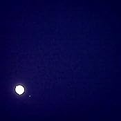
"Galileo Galilei constructed (1609) the first lens, or refracting,
telescope for astronomical purposes. Using several versions, he discovered
the four brightest Jovian satellites, lunar mountains, sunspots, the
starry nature of the Milky Way, and the apparent elongation of Saturn,
now known to be its rings. Galileo's simple lenses suffered from a
variety of aberrations, or defects of image formation: chromatic aberration,
or the variation of focal length with color; spherical aberration,
the variation of focal length with distance of parallel rays from
the lens axis; coma, the increasing blur of a point image with angle
of the rays to the axis; and distortion, the imaging of straight lines
in the object as curves. These aberrations were minimized in a variety
of ways. Christiaan Huygens constructed extremely long aerial telescopes
in which the objective lens was mounted on a pole and connected to
the eyepiece by only a taut wire. Despite extraordinary difficulties,
such instruments achieved useful results, especially in lunar mapping.''
These instruments have progressed far beyond the simple devices described above, but our study will deal only with the basic versions, using only convex (converging) lenses.
Theory: There are two principles essential to these instruments. First; light bends when moving from one medium to another. Second; the image formed by one lens can be the object for another.1) The whys of the bending of light were described in a previous lab. However, that experiment dealt with planar surfaces. A lens has at least one spherical section as a surface. With planar or rectangular lenses the exit light ray is parallel to the incident ray; it is merely offset. See figure 1:

fig. 1
On the other hand, when a ray of light is incident on a spherical lens it is redirected. According to Snell's law the ray must be bent toward the normal when traveling from a less to a more optically dense medium. The normal is drawn tangent to the surface of the lens where the ray enters. See figure 2a. When the ray exits to a less optically dense medium it is bent away from the normal drawn to the tangent. See figure 2b. 
fig. 2
The effect is to focus parallel rays of light to a point. See figure 3:

fig. 3
Moreover, due to symmetry, if the rays originate from a point the lens will cause them to be parallel; merely reverse the rays direction in figure 3. (There is a great deal of symmetry between telescopes and microscopes: one is the conjugate of the other.)
How much of a change of direction the light rays experience is dependent upon the curvature of the lens surface. Greater curvature causes greater bending. Lenses are normally characterized by the amount of bending, not by their curvature. Where two incident parallel rays which are subsequently bent cross is called the focal point, and the distance from the lens to this point is called the focal length. We rate lenses by their focal length, as in a long or a short focal length lens. Microscopes and telescopes employ both.One can determine a focal length (f) by examining the distance (s) to an object seen through the lens and the distance (s') to the image formed. A simple equation, called the lensmakers' equation, generates the focal length:

eq. 1
It will be necessary to ascertain the focal lengths of the various lenses you will use. N.B.: Some texts replace s and s' with p and q; be flexible! 2) Unlike most human beings, a lens doesn't know if what it `sees' is a physical reality or a mere projection. Therefore if one lens produces an image a second lens can treat this as an object. The difference between a microscope and a telescope is where the object for that first lens, called the objective, is in relation to the lens. This relation determines where the image formed by the first lens will be formed. For instance, if the object for the first lens is a long way away, the image will be formed on the opposite side of the lens. When, for a converging lens, the image is formed on the opposite side of the lens from the object s' is positive. You can verify this with equation 1: make s > f. On the other hand, if the object is close to the lens, the image will be formed on the same side of the lens as the object. Here s' < 0.
A small image (or object) one meter away emits (or reflects) light in parallel rays to your eyes. Your eye is most comfortable viewing objects perhaps a meter away; there is little strain to see detail and the image is clear. Optical instruments should therefore produce an image to your eye that is about one meter distant (a ballpark figure).
Now the obvious difference between the function of a microscope and the function of a telescope is that the former views small things close up and the latter views large things far away. In both cases we want a comfortable image for the viewer's eye. For these reasons a microscope uses a short focal length objective and a telescope uses a long focal length objective.
With a microscope we place a sample close to a short focal length lens, just beyond its focal point. This produces an image on the other side of the objective. We then use a second, longer focal length lens, called the eyepiece, to view this image. The image formed by the objective is just inside the focal length of the eyepiece. The image the eyepiece forms is therefore in front of the lens. This serves the purpose of moving the "virtual'' object the eye sees to a comfortable distance while magnifying it. (Magnification for a single lens is determined by the negative ratio of s' to s, or alternatively, the height of the image to the height of the object). The spacing (L) between the lenses is critical; L must be slightly less than s' (for the objective) plus f for the eyepiece. Since s is approximately equal to f for the objective, with the lensmakers' equation and f for the eyepiece L can be determined. Small adjustments to focusing are made by small variations in L.
A telescope works in the opposite manner. The long focal length objective forms its image such that s' = f for the objective. This is due to the fact that s is infinite (or close enough) for a telescope. The eyepiece, a shorter focal length lens, focuses on this image. The distance between the lenses is exactly the sum of the two lenses' focal lengths, so s = f for the eyepiece. The eye sees an image at infinity (greater than a meter), which is a comfortable viewing position. The magnification in a telescope is the ratio of the focal lengths (objective over eyepiece obviously).
There are other kinds of microscopes and telescopes--electron microscope, reflecting telescope--but we will restrict ourselves to 'scopes explained above.
Task:
Build a microscope
Build a telescope
Equipment:
- lenses
- optic bench w/lens holders
Procedure:
- Determine the focal lengths of all lenses. Use the optic bench and the lensmakers' equation.
- Place both lenses on the optic bench some distance apart. Which lens is the eyepiece and which is the objective depends on the experiment performed.
- The scale drawings can be done either in a graphics program or just on paper with the scale shown.
-If you let the object distance go to infinity, finding the focal length should be easy.
Microscope:
- To find the magnifying power of the microscope you need a reference object of known size.
- We suggest that this object have gradations like a meterstick, although an actual meterstick won't do.
- Make a card with regularly ruled lines about 20cm long. The separation should be around 0.5cm.
- Aim your microscope at this card and adjust the focus by moving the lenses relative to each other.
- Describe this image in your report.
- Re-aim the `scope off to one side just a bit so that both the microscope's image and the card are side-by-side when viewed through the 'scope.
- Compare the ruled markings on the card with the view through the 'scope. There should be an obvious difference in the apparent spacing between lines.
- Suppose there are 6 marked lines for every 3 image lines. The magnification is therefore 6/3 or 2. Something like this:

- Determine the magnification of your microscope.
- Compare this with the theoretical value.
- Draw a scale ray diagram for your instrument.
Telescope:
- To find the magnifying power of the telescope you also need a reference object of known size. Try making a paper card with ruled markings which are barely discernible from around 3-5 or more meters away.
- Aim your telescope at this target and adjust the focus by moving the lenses relative to each other. Describe this image in your report.
- Re-aim the 'scope off to one side just a bit so that both the telescope's image and the target are side-by-side when viewed through the `scope.
- Compare the ruled markings on the target with the view through the 'scope. There should be an obvious difference in the apparent spacing between marks.
- Suppose there are 7 target marks for every 2 image marks. The magnification is therefore 7/2 or 3.5. (see the discussion above).
- Determine the magnification of your telescope.
- Compare this with your theoretical value.
- Draw a scale ray diagram for your instrument.
Questions:
- Why is it obvious that the magnification of a telescope is the ratio of the objective's focal length over the eyepiece's focal length, and not the other way around?
- Although prism binoculars contain converging lenses only, objects viewed with them are seen erect. Explain how this might be accomplished.
- Show the following is true if the two lenses are directly next to each other (touching):

XXX . V Optical and digital microscopic imaging techniques and applications in pathology
The conventional optical microscope has been the primary tool in assisting pathological examinations. The modern digital pathology combines the power of microscopy, electronic detection, and computerized analysis. It enables cellular-, molecular-, and genetic-imaging at high efficiency and accuracy to facilitate clinical screening and diagnosis. This paper first reviews the fundamental concepts of microscopic imaging and introduces the technical features and associated clinical applications of optical microscopes, electron microscopes, scanning tunnel microscopes, and fluorescence microscopes. The interface of microscopy with digital image acquisition methods is discussed. The recent developments and future perspectives of contemporary microscopic imaging techniques such as three-dimensional and in vivo imaging are analyzed for their clinical potentials.
1. Flash back of microscope development
More than 2000 years ago, around one century B.C., people already had discovered that one could view an enlarged image of a small object by using a transparent “lens” with a spherical shape. Although a single convex lens can magnify an object by more than ten times, it is quite insufficient for people clearly to observe the details of many small objectives [1]. Near the end of 16th century, Dutch eyeglass dealer, Janssen, and his son inserted several lenses into a cylinder and found that an object was enlarged significantly if viewed through this assembled cylinder. This was the first prototype of a modern microscope and telescope. Based on this accidental discovery, Janssen designed and assembled the first compound microscope that included two convex lenses. The basic concept of a compound microscope is that an object can be enlarged sequentially by two convex lenses.
While observing the soft-wood specimen using a microscope in 1665, the British scientist, Robert Hooke, surprisingly discovered that the specimen depicted a series of unique “elements.” Hooke named them “cells.” Years later, a new microscope designed and assembled by a Dutch scientist, Anthony van Leeuwenhoek, provided much higher magnification power, which enabled people to observe substantially more details of cells. Although it exceeded all precedent microscopes, it was not another compound microscope and actually used only one convex lens. However, due to Leeuwenhoek's excellent manufacturing skill, this specially manufactured single convex lens achieved more than 300 times of magnification power.
In the following two centuries, the magnification power, as well as the image quality of the compound microscope, was improved substantially. This occurred, in particular, after the discovery and use of the new lens assemblies were able to eliminate or minimize the chromatic and other optical aberrations. Compared to the microscopes developed in 19th century, the conventional optical microscopes used to date have no substantial difference or improvement, because the optical microscopes have reached their maximum limitation in the spatial resolution.
Due to the large range or fluctuation of optical wavelength, it is impossible for any optical instruments to create a perfect image of a natural object, even if all shape defects in manufacturing optical lens were eliminated. Due to the unavoidable diffraction of optical wave passing through the microscopic lens, any point depicted on an object is no longer the point in the image plane but a diffraction spot. If two diffraction spots are too close together, the two points are not distinguishable. Under such circumstance, increasing magnification power of the microscopic objective lenses cannot further increase the spatial resolution of the microscopes. For the microscopes using the light sources within the range of visible optical wavelength, their spatial resolution is limited to 0.2 μm. Thus, any structures smaller than 0.2 μm cannot be distinguished using this type of microscope.
One approach to increasing spatial resolution of microscopes is to reduce optical wavelength or use electron beam to replace visible light source. According to the de Broglie theory of matter wave, moving electrons is similar in nature to optical wave fluctuation. The faster that electrons move, the shorter the “wavelength” of the released energy. If the electrons can be accelerated sufficiently and the released energy can be converged, the moving electron beam also can enlarge the objects. Based on this concept, German engineers, Max Knoll and Ernst Ruska, assembled the first transmission electron microscope (TEM) in the world in 1938 [2]. British engineer, Charles Oatley, manufactured the first scanning electron microscope (SEM) in 1952 [3]. Electron microscopy was one of the most important inventions in 20th century. Because electrons can be accelerated to very high speed, the spatial resolution of electron microscopes reaches up to 0.3 nm. As a result, many invisible materials (i.e., virus) under the visible light become “visible” under the electron microscope.
In 1983, two scientists in IBM laboratory, Gerd Binning and Heinrich Rohrer, invented the scanning tunnel electron microscope (STM) [4]. This advanced microscope was built using totally different concepts than those used by the conventional microscopes. STM works based on the so called “tunnel effect”. STM has no lens; rather, it uses a probe. Once the voltage is added between the probe and the observed object, the tunnel effect occurs if the distance between the probe and the surface of the observed objects is sufficiently small (i.e., measured in nanometers). When the electrons pass through the tiny space between the probe and the object, weak electronic current is generated. If the distance between the probe and the object varies, the strength of the current varies as well. Hence, the three-dimensional shape of the object can be detected as one measures the electronic current change. The spatial resolution of the STM can reach the level of a single atom.
2. The basic concept of microscopic imaging
Although many different types of microscopes have been developed, the basic imaging concept and structures can be simply illustrated in Fig. 1. The optical system of a microscope mainly includes an objective lens and eyepieces. The purpose of an objective lens is to magnify an object so that it can be clearly observed by the user. During the observation, the specimen is placed near the focal plane of the objective lens in the object space, and a magnified real image of specimen is first created on the intermediate plane. The intermediate plane is located on the focal plane of the eyepiece, thus the eyepiece is working as a magnifier to further magnify the image projected on the intermediate image plane. Finally, a magnified, virtual, inverted image is provided for the observer.

For a well designed microscope, the spatial resolution is mainly determined by the objective lens. Although an eyepiece can also magnify the image, it cannot improve the resolving power of the microscopes. The spatial resolution of an optical microscope is given by the Rayleigh equation as follows [5]:
Δr0 = 0.62λ ∕ n sin α
(1)
In the case of digital microscopic systems, the image magnified by the objective lens is directly acquired (or through a relay lens) by electronic detectors such as CCD or CMOS detectors [6, 7]. The electronic detectors are selected so that their pixel pitch is smaller than the magnified minimum resolvable distance determined by the objective lens. So that the resolving power of the microscope is not degraded by the digital detectors.
Based on the above equation, and considering the following practical limitations, (1) the use of visible light with the wavelength between 390 nm and 760 nm, (2) the maximally reachable aperture with the half-angle of 70–75 degree, and (3) the requirement of using immersion methods with water or oil to increase of refractive index, the resolution of a conventional optical microscope cannot exceed 200 nm.
Since the wavelength of electronic wave (beam) is much shorter than the visible light waves in several orders of magnitude, the resolution of a microscope using electronic beam in theory can reach approximately 0.3 nm. For this reason, electron microscopy [8, 9] is developed based on the principles of electronic optics, which can image the fine structure of objects at very high magnification power by using the electron beam and electron lens instead of optical lens. The transmission electron microscope (TEM) is the primary representation of the electron microscopes. The TEM is so named because the electron beam first penetrates the sample and then is magnified by the electronic imaging lens to produce the images. Its optic path is similar to the conventional optical microscope (as shown in Fig. 2). After passing through convergent lens, the parallel electron beam reaches the sample. Once the electron beam passes through the sample, it carries the information related to the sample characteristics. An electronic image is first generated once the electron beam passes though the objective lens and contrast aperture. After the electronic image is magnified again by the intermediate lens and projection lens, the final electron image is displayed in the electronic monitor screen. The contrast of the electron image is determined by the scattering level of electron beam once it interacts with the atoms in the sample. The electron beam also scatters less in the thinner samples or some parts with lower density. Thus, more electrons pass through lens aperture and result in the brighter image. On the other hand, thicker samples or denser parts appear darker in the image. If the sample is too thick or too dense, the image contrast is decreased substantially.

3. The microscopes used in biomedical fields
Although a large number of different types of microscopes have been developed and applied in different applications, the microscopes actually can be divided into three categories: (1) optical microscopes, (2) electron microscopes, and (3) scanning tunnel electron microscopes based on the microscope development history.
3.1. Optical microscopes
The simplified optical wave path of a conventional optical microscope is illustrated in Fig. 3. The modern optical microscope is able to magnify an object by 1500 times with the 0.2 μm limit in spatial resolution. The optical microscopes can be divided into many different types using a variety of criteria. For example, based on a lighting method, there are the transmission and reflection types of microscopes. In a transmission microscope, the light passes through transparent objects. In a refection microscope, the light source installed on the top of the microscopic lens illuminates the non-transparent objects, and the reflected light is collected by the lens. The microscopes can also be differentiated based on the observation methods, including bright field microscopes, dark field microscopes, phase difference microscopes, polarized light microscopes, interference microscopes, and fluorescent microscopes [5, 10–13]. Each microscope can use either the transmission or reflection approach. The bright field microscopes are the most popular and widely used of all microscopes. Using this type of microscope, the transmission (or absorption) ratio and reflection ratio of some observed objects vary according to the change of working environments. The amplitude of these objects varies with the change in lighting intensity. The colorless transparent objects are visible only when the phase of illuminated light changes. Because the bright field microscopes cannot change light phase, the colorless transparent specimens are invisible when using this type of microscope.

3.2. Electron microscopes
The resolution of the electron microscopes typically is represented by the small distance of two adjacent and distinguishable points. In the 1970s, transmission electron microscopes were able to reach the resolution of 0.3 nm, while the resolution limit of the human eye is around 0.1 mm. Compared to the optical microscopes that have the maximum magnification power of a few thousand times, the modern electron microscopes can increase the maximum magnification power to more than 300 million times. Using electron microscopes, one can directly observe some biological structures and/or the atomic structures of cells. Despite having superior spatial resolution over the optical microscopes, electron microscopes must work under the vacuum environment. Thus, they cannot be used to observe living biology samples. In addition, the electron beam can damage the illuminated specimens. Other issues (i.e., the optimal control of brightness of electron bean gun and the improvement of electron lens quality) still need investigations [14].
3.3. Scanning tunnel microscopes
The scanning tunnel microscope (STM) is also named “tunnel scanning microscope”. This instrument detects the surface structure of the objects based on the tunnel effect of the quantum mechanics. STM applies a very thinning tip (in an atom unit of its head) to detect the sample surface. As the tip is very close to the sample surface (<1 nm), the atoms in the tip head overlap with the electronic cloud of electrons in the sample surface. If a biasing voltage is applied between the tip and the samples, electrons will pass through the barrier between the tip and sample to generate the tunnel current in the order of nano-amperes (10−9 A). By controlling the distance between the tip and the sample surface and accurately moving the tip along the sample surface in the three-dimension, the detector can record the data related to the surface morphology, electronic surface states, and other relevant sample surface information [15]. The STM has the amazing ability to achieve the spatial resolution of less than 0.1 nm in the horizontal direction and less than 0.001 nm in vertical direction. Generally, when objects are in the solid state, the distance between atoms typically is from 0.001 nm to 0.1 nm. Because of this, the STM enables scientists to locate the single atom and observe the status of the atoms and molecules in the conductive material and surface structure. Hence, the STM generates substantially higher spatial resolution than other similar atomic microscopes. On the other hand, STMs can use the tip of the probe needle to manipulate accurately the atoms under low temperature environment. This enables the STM to be used as both a measurement and a process tool in the nanometer technology [16–18]. One unique characteristic of STM is that, for the first time, one can observe the permutation status of the atoms in the object surface and the related physical chemistry characteristics of the electrons in the surface. Due to the width and scope of its perspectives in the research and application fields related to the surface, material, and life sciences, the invention of the STM was considered by the international scientific community as one of the ten most important achievements of the science and technology in 1980s.
In summary, increasing microscope resolution has been an actively pursued goal in the microscopic imaging field. Using these three types of microscopes, one may observe the biological cells and microorganisms using an optical microscope, observe virus using an electron microscope, and detect or visualize the atoms using a scanning tunneling microscope.
3.4. Fluorescence microscopes
Although the fluorescence microscope can be characterized as a branch of the optical microscopes, it has many unique image generation and application characteristics in the biomedical imaging research fields. This section discusses this in more detail. The fluorescence microscope [19] uses short-wave light to illuminate the examined specimen and make certain objects inside the specimen emit the fluorescent light. Based on the received fluorescent light, one is able to observe the shape and location of the target objects. Comparing the difference between the fluorescence and conventional optical microscopes, one of the major differences is that the fluorescence microscope uses the high-voltage mercury lamp to provide all band light illumination, using a projection method in which the light is projected to the specimen. Due to the typically weakly reflected fluorescent light, the microscope must have a large numerical aperture to allow the objects to be observed. As a result, the numerical aperture of the fluorescent microscopes is larger than conventional optical microscopes. The fluorescent microscopes also have a special filtering system, including the assembly of the illumination filters and cut-off filters. Specifically, the fluorescent microscope has the following unique characteristics or requirements:
- 1)It requires a light source that has sufficient power to emit fluorescent light;
- 2)It is equipped with a set of optical filters that fit the requirement of stimulating different objects to emit different fluorescent light. By selecting the suitable wavelength of the emitting light, the wavelength of the emitted light can coincide with that of the absorption light, resulting in the maximum fluorescent light output;
- 3)To acquire the weak fluorescent images, it is equipped with a set of cut-off light filters that allow only the selected fluorescent light to pass through the imaging system and block the other types of scattering light to increase the signal-to-noise ratio of the system; and
- 4)The system of optical magnification needs to fit the characteristic of the fluorescent light in order eventually to obtain the fluorescent images with the highest spatial resolution.
Due to these requirements, a modern fluorescent microscope typically is assembled based on the structure of a duplex optical microscope. The equipped fluorescent device includes fluorescent light source, emission light path, stimulation/emission light filters, and the other components.
- 1)The fluorescent light source: It provides the light source that emits the light within the specific range of the wavelength or energy, which guarantees that the examined specimen acquires sufficient stimulation and generates strong fluorescent light. The fluorescent microscope typically uses the mercury lamp as the light source that is able to provide the exciting light with continuous wavelength. The mercury lamp has stronger energy in several commonly used light wavelengths (including 365 nm, 405 nm, 550 nm, and 600 nm).
- 2)An exciting light path: It serves as a fluorescent lighting device that contains a group of condenser lens and light focusing adjustment device. In the light path, the adjustable light and field apertures, (Neutral Density) ND filters, light splitter, and processing lens are installed.
- 3)Light filters: These are a set of the optical filtering components. Each has a certain wavelength width that selectively allows stimulated/emitted light pass through the optical system of the microscope.
Similar to the other conventional optical microscopes, the fluorescence microscopes can be divided into two categories based on their optical path [20]: transmission fluorescence microscopy (TFM) and epifluorescence microscopy. In TFM, the light passes through the condenser to excite the specimens to emit the fluorescence light. The TFM often uses the dark-field condenser that is able to adjust a reflector so that the light can illuminate the specimen from different directions. Compared to the old style fluorescent microscopes, the TFM has a number of advantages, which include producing strong fluorescence light when the specimen is observed in the low magnification. Disadvantages include the fact that as magnification levels increase, the fluorescence light weakens. Therefore, TFM is better used for observing larger specimens. As shown in Fig. 4, the light is emitted from one side of the specimen and the fluores-cent light is collected by the lens in the other side of the specimen.

The recently developed epifluorescence microscopy is a new type of fluorescent microscopy [21]. The difference between the epifluorescence and the transmission fluorescence microscopy is that the objective lens in epifluorescence microscope serves first as a well-corrected condenser and then as the imageforming light gatherer. The illuminator directs light onto the specimen by first passing the light through the microscope objective lens on the way toward the specimen and then using the same objective lens to capture the emitted light. The dichroic beam splitter is placed between the optical path titled at 45°, and the reflected excitation light passes through the objective lens and eventually reaches the specimen. The fluorescent light emitted by the specimen, as well as the reflected exciting or scattering lights, passes through the objective lens simultaneously and arrives at the dichroic separator (mirror) that separates the fluorescent light and the original exciting light. The remaining scattering light is absorbed further by the cut-off filter. The advantages of the epifluorescence microscope include the uniform illumination, sharp image, and the strong fluorescent light as the increase of the magnification level.
The optical path of an epifluorescence microscope is illustrated in Fig. 5. After the reflection from the dichroic mirror, the excitation light converges at the specimen. The emitted fluorescent light from the specimen first passes through the objective lens and the dichroic mirror, and then is collected by detection sensor (probes). The key component of an epifluorescence microscope is the dichroic beam splitter. It includes a multilayer optical interference filter that is installed with a titled angle of 45° along the optical path. It is able selectively to reflect or transmit the light only in certain wavelength range.

Although the transmission fluorescence microscopes can yield images with sufficiently high contrast in low magnification, the image is often relatively dark compared to the use of the epifluorescence microscope. Thus, the epifluorescence microscope is more popular in clinical practice to date. In addition, compared to the transmission fluorescence microscope, the epifluorescence microscope has following characteristics.
- 1)The microscope objective lens also serves as a light condenser. Thus, the alignment issue of the condenser is avoided. In particular, the fluorescent light intensity of the image increases as the increase of the numerical aperture (NA) of the object.
- 2)Since excitation light does not pass through slides in epifluorescence microscopy, it reduces the light loss. Meanwhile, the excitation and fluorescent light travel in the opposite direction to the objective lens. Two light beams separate with each other without interference. Some scattered excitation light may reach the object, and they are mostly reflected by the dichroic mirror to the light source. Thus, a very thin filter typically is installed between the objective lens and the detector (probe) to absorb a small fraction of remaining scattering light passing through the objective lens.
- 3)Unlike the use of transmission-type of excitation, in which most of fluorescence light creates in the bottom section of the specimen and must transmit through the specimen slice producing unavoidable scatter light, in epifluorescence microscope, the light source and the observation plane locate in the same plane. Therefore, there is no loss of the fluorescence intensity and no effect on image quality. In particular, it has unique advantages when it is used to examine the thick specimen slices with bacteria and tissue culture.
- 4)Since the ultraviolet (UV) light needs to pass through the objective lens, the transmission coefficient of the objective lens must be considered. As a result, a series of special objective lenses that can transmit UV light have been designed and manufactured. However, such a special objective lens is not required in the transmission fluorescence microscope.
4. The application of microscopes in pathological imaging
The invention of the microscope has significantly promoted the development of biology and medicine. It demonstrates the mystery of the microscopic world and reveals the causes of disease from the microscopic view. By acquiring the microscopic and pathologic images of the pathogenic microorganisms, medical researchers have established a series of new academic subjects, including bacteriology, immunology, virology, cell pathology, and others. In particular, the invention of electron microscopes has raised the observation of the traditional pathology from the cellular level to the sub-cellular level. As a result, one cannot practice modern medicine without microscopes. New microscopes such as the confocal laser scanning microscope (CLSM) [22], atomic force microscope (AFM), and scanning tunneling microscopy (STM) further improve the resolution of pathology imaging [23]. In this section, we briefly discuss the application of microscopes in assisting the clinicians in biomedical engineering, particularly in diagnosing pathological images.
4.1. Optical microscopes
Optical microscopes have been used widely in the pathology related clinical laboratories to diagnose a variety of diseases based on the examination of the body fluid change, invaded virus, and the variation of atomic structures [24]. Such diagnostic information and reports provide the clinicians with valuable references to select and implement the optimal treatment plans for the patients and monitor their efficacy. In genetic engineering and microscopic surgery, microscopes are essential tools for clinicians. Although optical microscopes are still considered to be very important tools in the clinical facilities, the development of the originally optical microscopes is quite mature to date; in particular, the optical characteristics of the microscopes have reached perfect degree without much space left to make further improvement. Therefore, the current development of the optical microscopes focuses on finding new application fields, making the systems simple and easy to use, as well as making one system for the multiple applications.
Since the biological specimen is typically one kind of muddy medium, it can generate the strong light scattering and absorption. As a result, the light (or optical wave) cannot penetrate deeply into the interior of the biological structures; thus, it is unable to extract a clear image of the biological structures. With the rapid advance of photonics, new imaging methods based on photonics have been developed, including the laser confocal scanning microscope and the near-field optical scanning microscop [25, 26]. First, the laser confocal scanning microscope is the combination of laser source and the confocal microscope. Specifically, it is a system that uses both the confocal concept of the traditional optical microscopy and the laser as the light source. It then uses the computer to process and analyze the acquired digital images of the observed specimens. By continuously scanning the multiple layers of the living cells or tissue slices, the laser confocal scanning microscope can acquire the complete 3D images of each structural layer of a single cell or local structure of a group of cells. Based on the near-field probing theory, the near-field optical scanning microscopy is a new technology developed by using the optical scanning probe needles. It breaks through the limitation of optical diffraction and is able to reach the spatial resolution in the range from 10 nm to 200 nm. By further combining with the related optical spectroscopy, using the near-field optical scanning microscopy creates a new approach to detecting and examining spectrum images of small biological specimen beyond nanometer range. As a result, researchers are able to analyze the single biological atom to date.
4.2. Electron microscopes
There are number of differences between electronic and optical microscopes when applied to pathological images. When using optical microscopes to observe pathological specimens, the observer routinely needs to adjust the micro-focusing system of the microscope and move the specimen to achieve the optimal observation of the tissue structure of the specimen. Using optical microscopes also generates less eye fatigue due to small light simulation to the eyes. However, the magnification power of the optical microscope is much lower than that of the electronic microscope. In addition to the higher magnification power, an electronic microscope can display more detailed tissue structures on the monitor (screen). It also may be able to conduct secondary magnification of the specimen displayed on the screen. Thus, the electronic microscope plays an important role in studying human organ tissue structures and the other sub-nanometer structures.
Due to the short wavelength of the electron beams, the electrical microscopes break through the limitation of the spatial resolution using optical microscopes, which opened a new door for the human eyes to observe the small structures at the molecule and/or atomic level. For example, using electronic microscopes to observe cells, researchers clearly have confirmed the existence of a cell membrane that consists of three thin layers with equal thickness but different density. Two external layers have higher density than the middle (interior) layer. When using electronic microscopes to observe unmyelinated nerve fiber, it was found that the nerve membrane cell of the fiber contained multiple shafts (i.e., 2 to 9). When using electronic microscopes to observe and study muscle structure, researchers discovered two important characteristics of muscle fiber: (1) the muscle fiber depicts the horizontally bright and dark stripes in the regular arrangement (namely the structure of horizontal stripes), and (2) muscle fiber is actually formed by finer fiber units that are perpendicular to the main fiber. Using electronic microscopes to study atomic structure of nucleic acid, observers can identify the linear status inside the nucleic acid atom structure with diameter around 20A°. These examples indicate that the application of electronic microscopes significantly expedites the possibility of exploring the secret of life and also plays an important role in the advance of medicine, as well as the improvement of human health [27].
In pathology, electronic microscopes have showed their importance in many applications. For example, electronic microscopes have been applied to pathological diagnosis of renal biopsy specimens. Renal glomerular disorder is a commonly diagnosed disease in clinical practice and can be classified as primary and secondary types of disorders. In order to more accurately diagnose the pathology of renal glomerular disorder, renal needle biopsy often is used. Besides distinguishing the different patterns of the morphological and tissue elements inside glomeruli, electronic microscopes can be used to observe and detect micro-structural aberration or changes, especially in epithelial cells, mesenterium, base membrane, and interstitial substance, which cannot be observed or detected using the conventional optical microscopes. By analyzing the observed micro-changes, physicians can find whether there are electron-dense deposits and corresponding locations. However, the single electronic microscopic technology also has limitation. In order to make renal needle biopsy more useful and accurate in the pathology diagnosis, the combination of multiple technologies, including the optimal use of conventional optical microscopes, immune-fluorescence microscopes, and electronic microscopes, is needed [23].
Using the electronic microscope not only has improved and enhanced the knowledge of the pathology, but also has provided a reliable foundation for the diagnosis of many diseases. With the rapid advance of science and technology, electronic microscopes have been and will continue be extensively used in pathologic diagnosis. However, single electronic microscopic technology has some limitations in pathologic diagnosis. For example, the field of vision (FOV) is reduced substantially due to the high spatial resolution of the electron microscope. Each FOV typically can only show a single cell or the partial structure of the cell. Meanwhile, observers can only observe still and dead specimens instead of the cells in vivo. Therefore, while electronic microscopes have been used actively in clinical practice, one also needs to combine other technologies such as the quantitative analysis of the morphology of the micro-structural changes using image processing, the nucleic acid hybridization in situ technology, and the apoptotic indices of the observation using electronic microscopes. Meanwhile, the scanning tunnel microscope and the atomic force microscope also have been introduced recently into the pathological area to improve the electronic microscopic technology. With closer connections to computer technology, the observers (i.e., pathologists) more easily and conveniently can use and control electronic microscopes through the connected computer and networking systems.
4.3. Fluorescence microscopes
Irradiated by the short wavelengths of light (e.g., ultraviolet and violet blue light 250 nm–400 nm), some substances can be excited by absorbing the energy and emit a longer wavelengths of light with energy degradation, which includes blue, green, yellow, or red light within the wavelength between 400 nm and 800 nm. This is called photoluminescence [28]. Some specimens naturally can generate fluorescent light when they are illuminated by the light with the proper wavelength. For example, most lipid and protein can emit fluorescent light in blue. This phenomenon is called auto fluorescence or primary fluorescence. However, most substances generate fluorescence light only when they are dyed with fluorochromes and are exposed in the light of short wavelengths.
In the 1930s, florescent staining was applied to investigating and observing the morphology of bacteria, mildew, cells, and fiber. For example, Mycobacterium tuberculosis can be detected in sputum by acid– fast bacteria staining methods. In the 1940s, the fluorescent staining protein technology was invented and applied extensively to the routine clinical immuno-fluorescence staining, which can examine and locate virus, bacteria, mildew, protozoan, parasite, antigen, and antibody in animals and humans. It has been used to investigate the pathogenesis and the cause of diseases such as categorizing and diagnosing glomerular diseases and identifying the relation between human papillomavirus (HPV) and the cervical cancer. The fluorescence microscope, a special tool for detecting fluorescence, has been getting more and more applications in the clinical research and disease diagnosis [29]. The coupling system between a fluorescence microscope and a fluorescence spectrometer has been extensively used in cell biology, biochemistry, physiology, neurobiology, and pathology. These systems can provide qualitative and quantitative analysis for various structures in either living and fixed cells or tissues. Fluorescence microscopes can observe cells and structures either emitting auto fluorescent or stained by the fluorochromes. The light source of a fluorescent microscope is a high-voltage mercury lamp that emits the ultraviolet light with short wavelengths. The fluorescent microscope also is installed with excitation and dichroic filters. The fluorochromes in the specimens are excited by the ultraviolet light and emit light with different colors. This enables one to analyze the distribution and locations of fluorescence inside the cells or structures. Some tissues can emit auto or spontaneous fluorescent light. For example, lipofoscin inside nerve or myocardial cells emit brown fluorescent light; Vitamin A of epithelia cells in hepatic Ito and retinal pigment emit green fluorescent light; and monoamine (e.g., Catecholamine, 5 – HT, Histamine) inside neuroendocrine cells and nerve fibers emits light with different colors under formaldehyde. Quinine and Tetracycline inside the tissues also emit fluorescent light. Some tissues inside the cells can bind with fluorescein to emit fluorescent light. For example, Ethidium bromide and Acridine orange can combine with DNA to measure the content of DNA. The fluorescence microscope also has been widely used in the immunocytochemistry research. By using fluorochrome to mark Isothiocyanate and Rhodamine, the marked antibody directly or indirectly can bind with the corresponding antigen. Thus, clinicians can detect the existence and distribution of antigen.
Since the invention of first fluorescence microscope in 1908, fluorescence detection has been improving constantly. This includes the introduction of high-voltage mercury lamps and the development of the multi-layer coating technology that is able to manufacture the high quality excitation and cut-off filters. With high quality optical components, the fluorescent microscope made a great contribution to the development of immune-fluorescence in the 1980s. In the 1990s, the laser scanning confocal fluorescence microscopy was developed. It measures and determines the fluorescence distribution within cells and tissue biopsies and obtains real-time overlapping phase-contrast and fluorescence images, as well as the primary color images labeled with double fluorescents. Currently, more advanced technologies related to the single-photon fluorescence microscopy, two-photon fluorescence microscopy, 4 pi confocal fluorescence microscopy [30], and full internal reflection fluorescence microscopy [31] (total internal reflectance fluorescence microscopy) have been developed. As a result, using these new tools, the technology and application of fluorescence detection can be applied or implemented in more research and clinical applications in pathology and other biomedical fields.
5. Digital microscope imaging
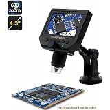
Although microscopy plays a very important role in biology and medicine, the observation is performed with the naked eye under the conventional optical microscopes. This can result in eye fatigue after a relatively long time of continuous observation. In addition, the image information cannot be stored and processed for different image enhancement purposes. To solve these limitations, digital microscopes have been developed and tested. A digital microscope (or imaging system) is an integrated design that combines traditional optical microscope, digital multimedia, and digital processing technology [32, 33]. As shown in Fig. 6, a digital microscope imaging system typically includes three components: Microscopy optical module, data acquisition module, digital image processing, and software control modules. Among these modules, the optical module realizes the function of the microscopic imaging; data acquisition module records the images produced by digital video devices, including CMOS, CCD, digital camera stored in optical module in the digital format, and then transfers these digital images to the computer storage devices through different graphics card interface or USB interface; and the software control module, the core of the whole system, controls the image capture, processing, and measurement in real-time to optimally improve the image quality. The digital images can be monitored in real-time using a color TV or computer monitors. After using a variety of digital image processing methods, digital microscopic imaging systems more sensitively can capture and display the image details. In fact, installation of online image acquisition, processing, and analysis systems have become an important symbol of modern advanced microscopes.

Due to its significantly technological advantages, microscopic digital imaging technology also has been used and/or integrated in a variety of electronic microscopes. For example, unlike the traditional electron microscopy imaging that uses electronic sensitive floor to generate photographic images, the digital microscope equipped with the CCD imaging system converts electrons that carry image information through electro-optical conversion devices to the light signal and sends the signal to the CCD. After the images are captured with CCD, they can be sent to the computer through an image acquisition card to perform a variety of required image processing procedures (as shown in Fig. 7).

The working principle of digital microscopic imaging system. 1 – Electron microscope lens; 2 – Fluorescence plate; 3 – Prism; 4 – Prism Block; 5 – Drive screw; 6 – Motor; 7 – Base; 8 – Aperture; ...
Thus, digital microscopic imaging technology is an extension of conventional microscopy. It integrates the microscopy, image acquisition, and computer control and processing technology to manage and control the whole imaging process, including image acquisition, sampling, processing, and data storage. Among these, the image acquisition and processing technology is the core for digital microscopic imaging technology.
Current digital image acquisition devices can be divided into three categories, including the use of (1) analog cameras plus video capture card, (2) consumer grade digital cameras, and (3) professional grade digital cameras. These three devices have their own characteristics and application fields in which professional grade digital cameras are the most popular choice in digital imaging microscopy systems. The introduction of digital imaging technology creates a great opportunity for the post-processing of acquired images. In particular, with the rapid advance of more powerful computers, digital microscopic images can be more effectively and efficiently processed and analyzed.
Image analysis and processing may be custom-designed or may use sophisticated commercial microscopic image processing software packages. Many professional software packages are well designed with variety of useful functions or schemes. They can provide both simple geometric measurement and sophisticated analysis to identify the relationship between the complex geometric structures. By providing the absolute space calibration to ensure the most accurate measurements and the advanced image segmenting technology, these commercial schemes can help observers to better distinguish the overlapping objects, detect the contours and shapes of the small objects, identify similar objects or groups, and categorize or mark the different objects with different colors. Some schemes can be used as advanced analytical tools that use the spectrum diagram, spectral profile, pseudo-color, three-dimensional surface shape, and other methods to manipulate the data and display it in different formats.
The advantage of connecting the microscope to a computer is that it produces digital images. Using these digital images, the research scientists and clinicians can apply various image processing and analysis software to obtain needed experimental data for variety of purposes. For example, using digital microscopes, one can replace the manual process of counting red tide organisms, a very tedious and time-consuming task. The computerized program is able to count the total number of red tide organisms depicted in a sample and classify red tide organisms in different size groups. The magnified red tide organisms can be displayed on the computer screen. As a result, by combining with manual identification, this computerized method greatly reduces the labor intensity of manual count using a conventional optical microscope.
6. New development in microscopic imaging technology
With the advance of technology and the special requirements of research projects, many new microscopic imaging methods have been developed and tested that aim to acquire the images with high resolution and large field of depth, as well as in three-dimensional stereoscopic format. As a result, using these new microscopic imaging systems and acquired images, the clinicians are able to conduct dynamic, non-destructive, and non-intervention in vivo (real time) tests in the biomedical research and clinical practice. Following are several new developments in this field.
6.1. Coexistence of a large field depth and high magnification power
In the conventional optical microscope, a large depth of field cannot coexist with high magnification power. As a result, due to the limited depth of field, the optical microscope cannot capture clear images of the targeted small objects located at different depths of the sample surface. The use of a scanning electron microscopy (SEM) or a confocal microscopy can resolve the contradiction between magnification and depth of field. As a result, one can observe clear (sharp) images with larger depth of field.
The SEM uses a very thin electronic beam to scan the sample surface. Electrons produced by scanning are collected by a specially designed detector. The corresponding electrical signals are further delivered to the CRT monitor screen to generate the three-dimensional image of the sample surface. These images also can be captured into the pictures. The resolution of the SEM lies between optical microscopy and transmission electron microscopy (TEM) (i.e., up to 3 nm). Meanwhile, the depth of field of the SEM is a hundred times higher than the optical microscope and at least ten times greater than the TEM. Thus, it is able to acquire a clear picture with a large depth of field.
The confocal microscope is an integrated technology that combines the optical and digital image analysis technique. It is a new microscopic imaging technology specifically useful in acquiring the images of non-planar samples. It can obtain enormous depth of field and exquisite details and also can acquire true-color information that often cannot be obtained using an electron microscope. When using the confocal microscope, one first adjusts the focus to search for and reach the samples distributed in different depth levels, captures all the images distributed in these levels with digital imaging devices, and transfers them to a computer (each of these aspects of the image has a clear location different from other images that record different parts of sample morphology and color information). After data analysis and integration using the special image processing software, the final high quality and clear picture is produced.
6.2. Three-dimensional imaging
The modern microscopy is not only limited to observing the specimen surface. By combining laser and confocal microscopy, researchers and clinicians can acquire and view the images of the cross sections of specimens at different depth levels. Then, using computerized image processing and 3D reconstruction algorithms, the three-dimensional shape profile of specimens can be acquired in high-resolution.
The main principle of laser scanning confocal microscope (LSCM) is to let the laser beam pass through a pinhole to generate a point light source. The laser light passes through the excitation filter and arrives at the beam splitter. Because the beam splitter can reflect excitation light with a shorter wavelength and transmit the light with a longer wavelength, the excitation light is reflected at the beam splitter and transmits through the objective lens. The laser beam scans different focal planes marked by the fluorescent agents under the control of the scanning control device. The excited emission light from the fluorescent marks passes through the original incident light path and directly returns to the beam splitter. After passing through the transmission filter for the specific wavelength, the emission light finally reaches the detection pinhole of the photomultiplier tube (PMT). By converting the PMT current into the digital signals, an image is created and displayed on the computer monitor screen.
Since LSCM can continuously scan the living cells and tissue or cell biopsy samples layer by layer to obtain images at different depth levels, it is also named as “non-destructive optical biopsy”. The distance between two LSCM scanned layers can be less than 0.1 um. Using computerized reconstruction algorithms, one can generate or acquire three-dimensional images that are able to observe or access the sophisticated cytoskeleton, chromosomes, organelles, and cell membrane.
6.3. In vivo detection
Observing and monitoring living cells can be very useful in many research applications, but it is a difficult technical challenge in the microscopic imaging field. To enable researchers or clinicians to observe the detailed structures of the specimens and also dynamically monitor the function of living cells or tissues in real-time using microscopic pathology images, several new technologies have been developed and tested. For example, by applying the specific fluorescence probes to label the material to be observed, the researchers can use LSCM to monitor dynamically the whole process of change in different locations or tissues of the cells after receiving stimulation in real time. LSCM also can be used in many applications such as assaying the changes within the PH of the cells, detect potential changes in membranes, detecting the production of intracellular reactive oxygen, testing the process of drugs into the tissue or cell membrane and locating its position, measuring the fluorescence resonance energy transfer (FRET), and real-time monitoring many other living cells.
7. Summary
Pathological imaging technology is a fast growing area of academic investigations, industrial developments and clinical applications. This paper presents a brief review of the fundamental concepts and a discussion on the recent developments and clinical potential of contemporary microscopic imaging techniques. The conventional optical microscopy has been an important tool in clinical pathology. The interface of optical microscopy with digital image acquisition methods combines the power of optical imaging, electronic detection, and computerized analysis. These and other emerging technologies will continue to evolve, enable cellular-, molecular-, and genetic-imaging, as well as tissue imaging with high efficiency and accuracy, to facilitate clinical screening and diagnosis.
XXX . V0 Optical telescope
An optical telescope is a telescope that gathers and focuses light, mainly from the visible part of the electromagnetic spectrum, to create a magnified image for direct view, or to make a photograph, or to collect data through electronic image sensors.
There are three primary types of optical telescope:
People use telescopes and binoculars for activities such as observational astronomy, ornithology, pilotage and reconnaissance, and watching sports or performance arts.

Eight-inch refracting telescope at Chabot Space and Science Center
The telescope is more a discovery of optical craftsmen than an invention of a scientist.[1][2] The lens and the properties of refracting and reflecting light had been known since antiquity and theory on how they worked were developed by ancient Greek philosophers, preserved and expanded on in the medieval Islamic world, and had reached a significantly advanced state by the time of the telescope's invention in early modern Europe.[3][4] But the most significant step cited in the invention of the telescope was the development of lens manufacture for spectacles,[2][5][6] first in Venice and Florence in the thirteenth century,[7] and later in the spectacle making centers in both the Netherlands and Germany.[8] It is in the Netherlands in 1608 where the first recorded optical telescopes (refracting telescopes) appeared. The invention is credited to the spectacle makers Hans Lippershey and Zacharias Janssen in Middelburg, and the instrument-maker and optician Jacob Metius of Alkmaar.[9]
Galileo greatly improved[citation needed] on these designs the following year, and is generally credited as the first to use a telescope for astronomy. Galileo's telescope used Hans Lippershey's design of a convex objective lens and a concave eye lens, and this design is now called a Galilean telescope. Johannes Kepler proposed an improvement on the design[10] that used a convex eyepiece, often called the Keplerian Telescope.
The next big step in the development of refractors was the advent of the Achromatic lens in the early 18th century,[11] which corrected the chromatic aberration in Keplerian telescopes up to that time—allowing for much shorter instruments with much larger objectives.
For reflecting telescopes, which use a curved mirror in place of the objective lens, theory preceded practice. The theoretical basis for curved mirrors behaving similar to lenses was probably established by Alhazen, whose theories had been widely disseminated in Latin translations of his work.[12] Soon after the invention of the refracting telescope Galileo, Giovanni Francesco Sagredo, and others, spurred on by their knowledge that curved mirrors had similar properties as lenses, discussed the idea of building a telescope using a mirror as the image forming objective.[13] The potential advantages of using parabolic mirrors (primarily a reduction of spherical aberration with elimination of chromatic aberration) led to several proposed designs for reflecting telescopes,[14] the most notable of which was published in 1663 by James Gregory and came to be called the Gregorian telescope,[15][16] but no working models were built. Isaac Newton has been generally credited with constructing the first practical reflecting telescopes, the Newtonian telescope, in 1668[17] although due to their difficulty of construction and the poor performance of the speculum metal mirrors used it took over 100 years for reflectors to become popular. Many of the advances in reflecting telescopes included the perfection of parabolic mirror fabrication in the 18th century,[18] silver coated glass mirrors in the 19th century, long-lasting aluminum coatings in the 20th century,[19] segmented mirrors to allow larger diameters, and active optics to compensate for gravitational deformation. A mid-20th century innovation was catadioptric telescopes such as the Schmidt camera, which uses both a lens (corrector plate) and mirror as primary optical elements, mainly used for wide field imaging without spherical aberration.
The late 20th century has seen the development of adaptive optics and space telescopes to overcome the problems of astronomical seeing.

Resolving power is derived from the wavelength using the same unit as aperture; where 550 nm to mm is given by: .
The constant is derived from radians to the same unit as the objects apparent diameter; where the Moons apparent diameter of radians to arcsecs is given by: .
An example using a telescope with an aperture of 130 mm observing the Moon in a 550 nm wavelength, is given by:
The unit used in the object diameter results in the smallest resolvable features at that unit. In the above example they are approximated in kilometers resulting in the smallest resolvable Moon craters being 3.22 km in diameter. The Hubble Space Telescope has a primary mirror aperture of 2400 mm that provides a surface resolvability of Moon craters being 174.9 meters in diameter, or sunspots of 7365.2 km in diameter.
The Rayleigh criterion for the resolution limit (in radians) is given by
For large ground-based telescopes, the resolution is limited by atmospheric seeing. This limit can be overcome by placing the telescopes above the atmosphere, e.g., on the summits of high mountains, on balloon and high-flying airplanes, or in space. Resolution limits can also be overcome by adaptive optics, speckle imaging or lucky imaging for ground-based telescopes.
Recently, it has become practical to perform aperture synthesis with arrays of optical telescopes. Very high resolution images can be obtained with groups of widely spaced smaller telescopes, linked together by carefully controlled optical paths, but these interferometers can only be used for imaging bright objects such as stars or measuring the bright cores of active galaxies.
An example of a telescope with a focal length of 1200 mm and aperture diameter of 254 mm is given by:
Numerically large Focal ratios are said to be long or slow. Small numbers are short or fast. There are no sharp lines for determining when to use these terms, an individual may consider their own standards of determination. Among contemporary astronomical telescopes, any telescope with a focal ratio slower (bigger number) than f/12 is generally considered slow, and any telescope with a focal ratio faster (smaller number) than f/6, is considered fast. Faster systems often have more optical aberrations away from the center of the field of view and are generally more demanding of eyepiece designs than slower ones. A fast system is often desired for practical purposes in astrophotography with the purpose of gathering more photons in a given time period than a slower system, allowing time lapsed photography to process the result faster.
Wide-field telescopes (such as astrographs), are used to track satellites and asteroids, for cosmic-ray research, and for astronomical surveys of the sky. It is more difficult to reduce optical aberrations in telescopes with low f-ratio than in telescopes with larger f-ratio.
An example gathering power of an aperture with 254 mm compared to an adult pupil diameter being 7 mm is given by:
Light-gathering power can be compared between telescopes by comparing the areas of the two different apertures.
As an example, the light-gathering power of a 10 meter telescope is 25x that of a 2 meter telescope:
For a survey of a given area, the field of view is just as important as raw light gathering power. Survey telescopes such as the Large Synoptic Survey Telescope try to maximize the product of mirror area and field of view (or etendue) rather than raw light gathering ability alone.
Similar minor effects may be present when using star diagonals, as light travels through a multitude of lenses that increase or decrease effective focal length. The quality of the image generally depends on the quality of the optics (lenses) and viewing conditions—not on magnification.
Magnification itself is limited by optical characteristics. With any telescope or microscope, beyond a practical maximum magnification, the image looks bigger but shows no more detail. It occurs when the finest detail the instrument can resolve is magnified to match the finest detail the eye can see. Magnification beyond this maximum is sometimes called empty magnification.
To get the most detail out of a telescope, it is critical to choose the right magnification for the object being observed. Some objects appear best at low power, some at high power, and many at a moderate magnification. There are two values for magnification, a minimum and maximum. A wider field of view eyepiece may be used to keep the same eyepiece focal length whilst providing the same magnification through the telescope. For a good quality telescope operating in good atmospheric conditions, the maximum usable magnification is limited by diffraction.
An example of visual magnification using a telescope with a 1200 mm focal length and 3 mm eyepiece is given by:
An example of the lowest usable magnification using a 254 mm aperture and 7 mm exit pupil is given by: , whilst the exit pupil diameter using a 254 mm aperture and 36x magnification is given by:
An example of true FOV using an eyepiece with 52° apparent FOV used at 81.25x magnification is given by:
An example of max FOV using a telescope with a barrel size of 31.75 mm (1.25 inches) and focal length of 1200 mm is given by:
Age plays a role in brightness, as a contributing factor is the observer's pupil. With age the pupil naturally shrinks in diameter; generally accepted a young adult may have a 7 mm diameter pupil, an older adult as little as 5 mm, and a younger person larger at 9 mm. The minimum magnification can be expressed as the division of the aperture and pupil diameter given by: . A problematic instance may be apparent, achieving a theoretical surface brightness of 100%, as the required effective focal length of the optical system may require an eyepiece with too large a diameter.
Some telescopes cannot achieve the theoretical surface brightness of 100%, while some telescopes can achieve it using a very small-diameter eyepiece. To find what eyepiece is required to get minimum magnification one can rearrange the magnification formula, where it is now the division of the telescope's focal length over the minimum magnification: . An eyepiece of 35 mm is a non-standard size and would not be purchasable; in this scenario to achieve 100% one would require a standard manufactured eyepiece size of 40 mm. As the eyepiece has a larger focal length than the minimum magnification, an abundance of wasted light is not received through the eyes.

where is the image scale, is the angular size of the observed object, and is the physical size of the projected image. In terms of focal length image scale is
where is measured in radians per meter (rad/m), and is measured in meters. Normally is given in units of arcseconds per millimeter ("/mm). So if the focal length is measured in millimeters, the image scale is
The derivation of this equation is fairly straightforward and the result is the same for reflecting or refracting telescopes. However, conceptually it is easier to derive by considering a reflecting telescope. If an extended object with angular size is observed through a telescope, then due to the Laws of reflection and Trigonometry the size of the image projected onto the focal plane will be
Thefore, the image scale (angular size of object divided by size of projected image) will be
and by using the small angle relation , when (N.B. only valid if is in radians), we obtain
Optical telescopes have been used in astronomical research since the time of their invention in the early 17th century. Many types have been constructed over the years depending on the optical technology, such as refracting and reflecting, the nature of the light or object being imaged, and even where they are placed, such as space telescopes. Some are classified by the task they perform such as Solar telescopes.
A new era of telescope making was inaugurated by the Multiple Mirror Telescope (MMT), with a mirror composed of six segments synthesizing a mirror of 4.5 meters diameter. This has now been replaced by a single 6.5 m mirror. Its example was followed by the Keck telescopes with 10 m segmented mirrors.
The largest current ground-based telescopes have a primary mirror of between 6 and 11 meters in diameter. In this generation of telescopes, the mirror is usually very thin, and is kept in an optimal shape by an array of actuators (see active optics). This technology has driven new designs for future telescopes with diameters of 30, 50 and even 100 meters.
Relatively cheap, mass-produced ~2 meter telescopes have recently been developed and have made a significant impact on astronomy research. These allow many astronomical targets to be monitored continuously, and for large areas of sky to be surveyed. Many are robotic telescopes, computer controlled over the internet (see e.g. the Liverpool Telescope and the Faulkes Telescope North and South), allowing automated follow-up of astronomical events.
Initially the detector used in telescopes was the human eye. Later, the sensitized photographic plate took its place, and the spectrograph was introduced, allowing the gathering of spectral information. After the photographic plate, successive generations of electronic detectors, such as the charge-coupled device (CCDs), have been perfected, each with more sensitivity and resolution, and often with a wider wavelength coverage.
Current research telescopes have several instruments to choose from such as:
In recent years, a number of technologies to overcome the distortions caused by atmosphere on ground-based telescopes have been developed, with good results. See adaptive optics, speckle imaging and optical interferometry.
There are three primary types of optical telescope:
- refractors, which use lenses (dioptrics)
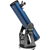
- reflectors, which use mirrors (catoptrics)
- catadioptric telescopes, which combine lenses and mirrors
People use telescopes and binoculars for activities such as observational astronomy, ornithology, pilotage and reconnaissance, and watching sports or performance arts.

Eight-inch refracting telescope at Chabot Space and Science Center
The telescope is more a discovery of optical craftsmen than an invention of a scientist.[1][2] The lens and the properties of refracting and reflecting light had been known since antiquity and theory on how they worked were developed by ancient Greek philosophers, preserved and expanded on in the medieval Islamic world, and had reached a significantly advanced state by the time of the telescope's invention in early modern Europe.[3][4] But the most significant step cited in the invention of the telescope was the development of lens manufacture for spectacles,[2][5][6] first in Venice and Florence in the thirteenth century,[7] and later in the spectacle making centers in both the Netherlands and Germany.[8] It is in the Netherlands in 1608 where the first recorded optical telescopes (refracting telescopes) appeared. The invention is credited to the spectacle makers Hans Lippershey and Zacharias Janssen in Middelburg, and the instrument-maker and optician Jacob Metius of Alkmaar.[9]
Galileo greatly improved[citation needed] on these designs the following year, and is generally credited as the first to use a telescope for astronomy. Galileo's telescope used Hans Lippershey's design of a convex objective lens and a concave eye lens, and this design is now called a Galilean telescope. Johannes Kepler proposed an improvement on the design[10] that used a convex eyepiece, often called the Keplerian Telescope.
The next big step in the development of refractors was the advent of the Achromatic lens in the early 18th century,[11] which corrected the chromatic aberration in Keplerian telescopes up to that time—allowing for much shorter instruments with much larger objectives.
For reflecting telescopes, which use a curved mirror in place of the objective lens, theory preceded practice. The theoretical basis for curved mirrors behaving similar to lenses was probably established by Alhazen, whose theories had been widely disseminated in Latin translations of his work.[12] Soon after the invention of the refracting telescope Galileo, Giovanni Francesco Sagredo, and others, spurred on by their knowledge that curved mirrors had similar properties as lenses, discussed the idea of building a telescope using a mirror as the image forming objective.[13] The potential advantages of using parabolic mirrors (primarily a reduction of spherical aberration with elimination of chromatic aberration) led to several proposed designs for reflecting telescopes,[14] the most notable of which was published in 1663 by James Gregory and came to be called the Gregorian telescope,[15][16] but no working models were built. Isaac Newton has been generally credited with constructing the first practical reflecting telescopes, the Newtonian telescope, in 1668[17] although due to their difficulty of construction and the poor performance of the speculum metal mirrors used it took over 100 years for reflectors to become popular. Many of the advances in reflecting telescopes included the perfection of parabolic mirror fabrication in the 18th century,[18] silver coated glass mirrors in the 19th century, long-lasting aluminum coatings in the 20th century,[19] segmented mirrors to allow larger diameters, and active optics to compensate for gravitational deformation. A mid-20th century innovation was catadioptric telescopes such as the Schmidt camera, which uses both a lens (corrector plate) and mirror as primary optical elements, mainly used for wide field imaging without spherical aberration.
The late 20th century has seen the development of adaptive optics and space telescopes to overcome the problems of astronomical seeing.
Principles
The basic scheme is that the primary light-gathering element the objective (1) (the convex lens or concave mirror used to gather the incoming light), focuses that light from the distant object (4) to a focal plane where it forms a real image (5). This image may be recorded or viewed through an eyepiece (2), which acts like a magnifying glass. The eye (3) then sees an inverted magnified virtual image (6) of the object.
Schematic of a Keplerian refracting telescope. The arrow at (4) is a (notional) representation of the original image; the arrow at (5) is the inverted image at the focal plane; the arrow at (6) is the virtual image that forms in the viewer's visual sphere. The red rays produce the midpoint of the arrow; two other sets of rays (each black) produce its head and tail.
Inverted images
Most telescope designs produce an inverted image at the focal plane; these are referred to as inverting telescopes. In fact, the image is both turned upside down and reversed left to right, so that altogether it is rotated by 180 degrees from the object orientation. In astronomical telescopes the rotated view is normally not corrected, since it does not affect how the telescope is used. However, a mirror diagonal is often used to place the eyepiece in a more convenient viewing location, and in that case the image is erect, but still reversed left to right. In terrestrial telescopes such as spotting scopes, monoculars and binoculars, prisms (e.g., Porro prisms) or a relay lens between objective and eyepiece are used to correct the image orientation. There are telescope designs that do not present an inverted image such as the Galilean refractor and the Gregorian reflector. These are referred to as erecting telescopes.Design variants
Many types of telescope fold or divert the optical path with secondary or tertiary mirrors. These may be integral part of the optical design (Newtonian telescope, Cassegrain reflector or similar types), or may simply be used to place the eyepiece or detector at a more convenient position. Telescope designs may also use specially designed additional lenses or mirrors to improve image quality over a larger field of view.Characteristics
Design specifications relate to the characteristics of the telescope and how it performs optically. Several properties of the specifications may change with the equipment or accessories used with the telescope; such as Barlow lenses, star diagonals and eyepieces. These interchangeable accessories don't alter the specifications of the telescope, however they alter the way the telescopes properties function, typically magnification, angular resolution and FOV.Surface resolvability
The smallest resolvable surface area of an object, as seen through an optical telescope, is the limited physical area that can be resolved. It is analogous to angular resolution, but differs in definition: instead of separation ability between point-light sources it refers to the physical area that can be resolved. A familiar way to express the characteristic is the resolvable ability of features such as Moon craters or Sun spots. Expression using the formula is given by the sum of twice the resolving power over aperture diameter multiplied by the objects diameter multiplied by the constant all divided by the objects apparent diameter .[20][21]


Resolving power is derived from the wavelength using the same unit as aperture; where 550 nm to mm is given by: .


The constant is derived from radians to the same unit as the objects apparent diameter; where the Moons apparent diameter of radians to arcsecs is given by: .


An example using a telescope with an aperture of 130 mm observing the Moon in a 550 nm wavelength, is given by:

The unit used in the object diameter results in the smallest resolvable features at that unit. In the above example they are approximated in kilometers resulting in the smallest resolvable Moon craters being 3.22 km in diameter. The Hubble Space Telescope has a primary mirror aperture of 2400 mm that provides a surface resolvability of Moon craters being 174.9 meters in diameter, or sunspots of 7365.2 km in diameter.
Angular resolution
Ignoring blurring of the image by turbulence in the atmosphere (atmospheric seeing) and optical imperfections of the telescope, the angular resolution of an optical telescope is determined by the diameter of the primary mirror or lens gathering the light (also termed its "aperture").The Rayleigh criterion for the resolution limit (in radians) is given by


For large ground-based telescopes, the resolution is limited by atmospheric seeing. This limit can be overcome by placing the telescopes above the atmosphere, e.g., on the summits of high mountains, on balloon and high-flying airplanes, or in space. Resolution limits can also be overcome by adaptive optics, speckle imaging or lucky imaging for ground-based telescopes.
Recently, it has become practical to perform aperture synthesis with arrays of optical telescopes. Very high resolution images can be obtained with groups of widely spaced smaller telescopes, linked together by carefully controlled optical paths, but these interferometers can only be used for imaging bright objects such as stars or measuring the bright cores of active galaxies.
Focal length and focal ratio
The focal length of an optical system is a measure of how strongly the system converges or diverges light. For an optical system in air, it is the distance over which initially collimated rays are brought to a focus. A system with a shorter focal length has greater optical power than one with a long focal length; that is, it bends the rays more strongly, bringing them to a focus in a shorter distance. In astronomy, the f-number is commonly referred to as the focal ratio notated as . The focal ratio of a telescope is defined as the focal length of an objective divided by its diameter or by the diameter of an aperture stop in the system. The focal length controls the field of view of the instrument and the scale of the image that is presented at the focal plane to an eyepiece, film plate, or CCD.

An example of a telescope with a focal length of 1200 mm and aperture diameter of 254 mm is given by:

Numerically large Focal ratios are said to be long or slow. Small numbers are short or fast. There are no sharp lines for determining when to use these terms, an individual may consider their own standards of determination. Among contemporary astronomical telescopes, any telescope with a focal ratio slower (bigger number) than f/12 is generally considered slow, and any telescope with a focal ratio faster (smaller number) than f/6, is considered fast. Faster systems often have more optical aberrations away from the center of the field of view and are generally more demanding of eyepiece designs than slower ones. A fast system is often desired for practical purposes in astrophotography with the purpose of gathering more photons in a given time period than a slower system, allowing time lapsed photography to process the result faster.
Wide-field telescopes (such as astrographs), are used to track satellites and asteroids, for cosmic-ray research, and for astronomical surveys of the sky. It is more difficult to reduce optical aberrations in telescopes with low f-ratio than in telescopes with larger f-ratio.
Light-gathering power
The light-gathering power of an optical telescope, also referred to as light grasp or aperture gain, is the ability of a telescope to collect a lot more light than the human eye. Its light-gathering power is probably its most important feature. The telescope acts as a light bucket, collecting all of the photons that come down on it from a far away object, where a larger bucket catches more photons resulting in more received light in a given time period, effectively brightening the image. This is why the pupils of your eyes enlarge at night so that more light reaches the retinas. The gathering power compared against a human eye is the squared result of the division of the aperture over the observer's pupil diameter ,[20][21] with an average adult having a pupil diameter of 7mm. Younger persons host larger diameters, typically said to be 9mm, as the diameter of the pupil decreases with age.

An example gathering power of an aperture with 254 mm compared to an adult pupil diameter being 7 mm is given by:

Light-gathering power can be compared between telescopes by comparing the areas of the two different apertures.

As an example, the light-gathering power of a 10 meter telescope is 25x that of a 2 meter telescope:

For a survey of a given area, the field of view is just as important as raw light gathering power. Survey telescopes such as the Large Synoptic Survey Telescope try to maximize the product of mirror area and field of view (or etendue) rather than raw light gathering ability alone.
Magnification
The magnification through a telescope magnifies a viewing object while limiting the FOV. Magnification is often misleading as the optical power of the telescope, its characteristic is the most misunderstood term used to describe the observable world. At higher magnifications the image quality significantly reduces, usage of a Barlow lens—which increases the effective focal length of an optical system—multiplies image quality reduction.Similar minor effects may be present when using star diagonals, as light travels through a multitude of lenses that increase or decrease effective focal length. The quality of the image generally depends on the quality of the optics (lenses) and viewing conditions—not on magnification.
Magnification itself is limited by optical characteristics. With any telescope or microscope, beyond a practical maximum magnification, the image looks bigger but shows no more detail. It occurs when the finest detail the instrument can resolve is magnified to match the finest detail the eye can see. Magnification beyond this maximum is sometimes called empty magnification.
To get the most detail out of a telescope, it is critical to choose the right magnification for the object being observed. Some objects appear best at low power, some at high power, and many at a moderate magnification. There are two values for magnification, a minimum and maximum. A wider field of view eyepiece may be used to keep the same eyepiece focal length whilst providing the same magnification through the telescope. For a good quality telescope operating in good atmospheric conditions, the maximum usable magnification is limited by diffraction.
Visual
The visual magnification of the field of view through a telescope can be determined by the telescopes focal length divided by the eyepiece focal length (or diameter). The maximum is limited by the diameter of the eyepiece.

An example of visual magnification using a telescope with a 1200 mm focal length and 3 mm eyepiece is given by:

Minimum
There is a lowest usable magnification on a telescope. The increase in brightness with reduced magnification has a limit related to something called the exit pupil. The exit pupil is the cylinder of light coming out of the eyepiece, hence the lower the magnification, the larger the exit pupil. The minimum can be calculated by dividing the telescope aperture over the exit pupil diameter .[22] Decreasing the magnification past this limit cannot increase brightness, at this limit there is no benefit for decreased magnification. Likewise calculating the exit pupil is a division of the aperture diameter and the visual magnification used. The minimum often may not be reachable with some telescopes, a telescope with a very long focal length may require a longer-focal-length eyepiece than is possible.

An example of the lowest usable magnification using a 254 mm aperture and 7 mm exit pupil is given by: , whilst the exit pupil diameter using a 254 mm aperture and 36x magnification is given by:


Optimum
A useful reference is:- For small objects with low surface brightness (such as galaxies), use a moderate magnification.
- For small objects with high surface brightness (such as planetary nebulae), use a high magnification.
- For large objects regardless of surface brightness (such as diffuse nebulae), use low magnification, often in the range of minimum magnification.
Field of view
Field of view is the extent of the observable world seen at any given moment, through an instrument (e.g., telescope or binoculars), or by naked eye. There are various expressions of field of view, being a specification of an eyepiece or a characteristic determined from and eyepiece and telescope combination. A physical limit derives from the combination where the FOV cannot be viewed larger than a defined maximum, due to diffraction of the optics.Apparent
Apparent FOV is the observable world observed through an ocular eyepiece without insertion into a telescope. It is limited by the barrel size used in a telescope, generally with modern telescopes that being either 1.25 or 2 inches in diameter. A wider FOV may be used to achieve a more vast observable world given the same magnification compared with a smaller FOV without compromise to magnification. Note that increasing the FOV lowers surface brightness of an observed object, as the gathered light is spread over more area, in relative terms increasing the observing area proportionally lowers surface brightness dimming the observed object. Wide FOV eyepieces work best at low magnifications with large apertures, where the relative size of an object is viewed at higher comparative standards with minimal magnification giving an overall brighter image to begin with.True
True FOV is the observable world observed though an ocular eyepiece inserted into a telescope. Knowing the true FOV of eyepieces is very useful since it can be used to compare what is seen through the eyepiece to printed or computerized star charts that help identify what is observed. True FOV is the division of apparent FOV over magnification .[20][21]

An example of true FOV using an eyepiece with 52° apparent FOV used at 81.25x magnification is given by:

Maximum
Max FOV is a term used to describe the maximum useful true FOV limited by the optics of the telescope, it is a physical limitation where increases beyond the maximum remain at maximum. Max FOV is the barrel size over the telescopes focal length converted from radian to degrees.

An example of max FOV using a telescope with a barrel size of 31.75 mm (1.25 inches) and focal length of 1200 mm is given by:

Observing through a telescope
There are many properties of optical telescopes and the complexity of observation using one can be a daunting task; experience and experimentation are the major contributors to understanding how to maximize one's observations. In practice, only two main properties of a telescope determine how observation differs: the focal length and aperture. These relate as to how the optical system views an object or range and how much light is gathered through an ocular eyepiece. Eyepieces further determine how the field of view and magnification of the observable world change.Observable world
Observable world describes what can be seen using a telescope, when viewing an object or range the observer may use many different techniques. Understanding what can be viewed and how to view it depends on the field of view. Viewing an object at a size that fits entirely in the field of view is measured using the two telescope properties—focal length and aperture, with the inclusion of an ocular eyepiece with suitable focal length (or diameter). Comparing the observable world and the angular diameter of an object shows how much of the object we see. However, the relationship with the optical system may not result in high surface brightness. Celestial objects are often dim because of their vast distance, and detail may be limited by diffraction or unsuitable optical properties.Field of view and magnification relationship
Finding what can be seen through the optical system begins with the eyepiece providing the field of view and magnification; the magnification is given by the division of the telescope and eyepiece focal lengths. Using an example of an amateur telescope such as a Newtonian telescope with an aperture of 130 mm (5") and focal length of 650 mm (25.5 inches), one uses an eyepiece with a focal length of 8 mm and apparent field of view of 52°. The magnification at which the observable world is viewed is given by: . The true field of view requires the magnification, which is formulated by its division over the apparent field of view: . The resulting true field of view is 0.64°, allowing an object such as the Orion nebula, which appears elliptical with an angular diameter of 65 × 60 arcminutes, to be viewable through the telescope in its entirety, where the whole of the nebula is within the observable world. Using methods such as this can greatly increase one's viewing potential ensuring the observable world can contain the entire object, or whether to increase or decrease magnification viewing the object in a different aspect.


Brightness factor
The surface brightness at such a magnification significantly reduces, resulting in a far dimmer appearance. A dimmer appearance results in less visual detail of the object. Details such as matter, rings, spiral arms, and gases may be completely hidden from the observer, giving a far less complete view of the object or range. Physics dictates that at the theoretical minimum magnification of the telescope, the surface brightness is at 100%. Practically, however, various factors prevent 100% brightness; these include telescope limitations (focal length, eyepiece focal length, etc.) and the age of the observer.Age plays a role in brightness, as a contributing factor is the observer's pupil. With age the pupil naturally shrinks in diameter; generally accepted a young adult may have a 7 mm diameter pupil, an older adult as little as 5 mm, and a younger person larger at 9 mm. The minimum magnification can be expressed as the division of the aperture and pupil diameter given by: . A problematic instance may be apparent, achieving a theoretical surface brightness of 100%, as the required effective focal length of the optical system may require an eyepiece with too large a diameter.


Some telescopes cannot achieve the theoretical surface brightness of 100%, while some telescopes can achieve it using a very small-diameter eyepiece. To find what eyepiece is required to get minimum magnification one can rearrange the magnification formula, where it is now the division of the telescope's focal length over the minimum magnification: . An eyepiece of 35 mm is a non-standard size and would not be purchasable; in this scenario to achieve 100% one would require a standard manufactured eyepiece size of 40 mm. As the eyepiece has a larger focal length than the minimum magnification, an abundance of wasted light is not received through the eyes.

Exit pupil
The increase in surface brightness as one reduces magnification is limited; that limitation is what is described as the exit pupil: a cylinder of light that projects out the eyepiece to the observer. An exit pupil must match or be smaller in diameter than one's pupil to receive the full amount of projected light; a larger exit pupil results in the wasted light. The exit pupil can be derived with from division of the telescope aperture and the minimum magnification , derived by: . The pupil and exit pupil are almost identical in diameter, giving no wasted observable light with the optical system. A 7 mm pupil falls slightly short of 100% brightness, where the surface brightness can be measured from the product of the constant 2, by the square of the pupil resulting in: . The limitation here is the pupil diameter; it's an unfortunate result and degrades with age. Some observable light loss is expected and decreasing the magnification cannot increase surface brightness once the system has reached its minimum usable magnification, hence why the term is referred to as usable.


These eyes represent a scaled figure of the human eye where 15 px = 1 mm, they have a pupil diameter of 7 mm. Figure A has an exit pupil diameter of 14 mm, which for astronomy purposes results in a 75% loss of light. Figure B has an exit pupil of 6.4 mm, which allows the full 100% of observable light to be perceived by the observer.
Image Scale
When using a CCD to record observations, the CCD is placed in the focal plane. Image scale (sometimes called plate scale) describes how the angular size of the object being observed is related to the physical size of the projected image in the focal plane
where is the image scale, is the angular size of the observed object, and is the physical size of the projected image. In terms of focal length image scale is


where is measured in radians per meter (rad/m), and is measured in meters. Normally is given in units of arcseconds per millimeter ("/mm). So if the focal length is measured in millimeters, the image scale is
![{\displaystyle i(''/mm)={\frac {1}{f(mm)}}\left[{\frac {180\times 3600}{\pi }}\right].}](https://wikimedia.org/api/rest_v1/media/math/render/svg/8a4f5962857cd96f83c83dfd14e0308e7eefcb28)
The derivation of this equation is fairly straightforward and the result is the same for reflecting or refracting telescopes. However, conceptually it is easier to derive by considering a reflecting telescope. If an extended object with angular size is observed through a telescope, then due to the Laws of reflection and Trigonometry the size of the image projected onto the focal plane will be

Thefore, the image scale (angular size of object divided by size of projected image) will be

and by using the small angle relation , when (N.B. only valid if is in radians), we obtain


Imperfect images
No telescope can form a perfect image. Even if a reflecting telescope could have a perfect mirror, or a refracting telescope could have a perfect lens, the effects of aperture diffraction are unavoidable. In reality, perfect mirrors and perfect lenses do not exist, so image aberrations in addition to aperture diffraction must be taken into account. Image aberrations can be broken down into two main classes, monochromatic, and polychromatic. In 1857, Philipp Ludwig von Seidel (1821–1896) decomposed the first order monochromatic aberrations into five constituent aberrations. They are now commonly referred to as the five Seidel Aberrations.The five Seidel aberrations
- Spherical aberration
- The difference in focal length between paraxial rays and marginal rays, proportional to the square of the objective diameter.
- Coma
- A defect by which points appear as comet-like asymmetrical patches of light with tails, which makes measurement very imprecise. Its magnitude is usually deduced from the optical sine theorem.
- Astigmatism
- The image of a point forms focal lines at the sagittal and tangental foci and in between (in the absence of coma) an elliptical shape.
- Curvature of Field
- The Petzval field curvature means that the image, instead of lying in a plane, actually lies on a curved surface, described as hollow or round. This causes problems when a flat imaging device is used e.g., a photographic plate or CCD image sensor.
- Distortion
- Either barrel or pincushion, a radial distortion that must be corrected when combining multiple images (similar to stitching multiple photos into a panoramic photo).
Chromatic aberrations
- Longitudinal chromatic aberration: As with spherical aberration this is the same for axial and oblique pencils.
- Transverse chromatic aberration (chromatic aberration of magnification)
Astronomical research telescopes

Large reflectors
Nearly all large research-grade astronomical telescopes are reflectors. Some reasons are:- In a lens the entire volume of material has to be free of imperfection and inhomogeneities, whereas in a mirror, only one surface has to be perfectly polished.
- Light of different colors travels through a medium other than vacuum at different speeds. This causes chromatic aberration.
- Reflectors work in a wider spectrum of light since certain wavelengths are absorbed when passing through glass elements like those found in a refractor or catadioptric.
- There are technical difficulties involved in manufacturing and manipulating large-diameter lenses. One of them is that all real materials sag in gravity. A lens can only be held by its perimeter. A mirror, on the other hand, can be supported by the whole side opposite to its reflecting face.

A new era of telescope making was inaugurated by the Multiple Mirror Telescope (MMT), with a mirror composed of six segments synthesizing a mirror of 4.5 meters diameter. This has now been replaced by a single 6.5 m mirror. Its example was followed by the Keck telescopes with 10 m segmented mirrors.
The largest current ground-based telescopes have a primary mirror of between 6 and 11 meters in diameter. In this generation of telescopes, the mirror is usually very thin, and is kept in an optimal shape by an array of actuators (see active optics). This technology has driven new designs for future telescopes with diameters of 30, 50 and even 100 meters.

Initially the detector used in telescopes was the human eye. Later, the sensitized photographic plate took its place, and the spectrograph was introduced, allowing the gathering of spectral information. After the photographic plate, successive generations of electronic detectors, such as the charge-coupled device (CCDs), have been perfected, each with more sensitivity and resolution, and often with a wider wavelength coverage.
Current research telescopes have several instruments to choose from such as:
- imagers, of different spectral responses
- spectrographs, useful in different regions of the spectrum
- polarimeters, that detect light polarization.
In recent years, a number of technologies to overcome the distortions caused by atmosphere on ground-based telescopes have been developed, with good results. See adaptive optics, speckle imaging and optical interferometry.
XXX . V00 Amateur telescope making
Amateur telescope making is the activity of building telescopes as a hobby, as opposed to being a paid professional. Amateur telescope makers (sometimes called ATMs) build their instruments for personal enjoyment of a technical challenge, as a way to obtain an inexpensive or personally customized telescope, or as a research tool in the field of astronomy. Amateur telescope makers are usually a sub-group in the field of amateur astronomy.

A 22" Newtonian reflector sits in front of the clubhouse at Stellafane, home of the Springfield Telescope Makers
Beginnings
Ever since Galileo took a Dutch invention and adapted it to astronomical use, astronomical telescope making has been an evolving discipline. Many astronomers after the time of Galileo built their own telescopes out of necessity, but the advent of amateurs in the field building telescopes for their own enjoyment and education seems to have come into prominence in the 20th century.Before the advent of modern mass-produced telescopes the price of even a modest instrument was often beyond the means of an aspiring amateur astronomer. Building your own was the only economical method to obtain a suitable telescope for observing. There were many published works that helped spark an interest in building telescopes such as Irish telescope maker Rev. W. F. A. Ellison's 1920 book "The Amateur's Telescope".
In the United States in the early 1920s articles in Popular Astronomy by Russell W. Porter and in Scientific American by Albert G. Ingalls featuring Porter and the Springfield Telescope Makers[1] helped expand interest in the hobby. There was so much public interest Ingalls began a regular column for Scientific American on the subject (spawning that publications The Amateur Scientist column) and later compiled into three books titled Amateur Telescope Making Vol. 1-3. These had a large readership of enthusiast (sometimes called "telescope nuts"[2]) constructing their own instruments. Between 1933 and 1990, Sky and Telescope magazine ran a regular column called "Gleanings for ATMs" edited by Earle Brown, Robert E. Cox & Roger Sinnott. The ready supply of surplus optical components after World War 2 and later Sputnik and the space race also greatly expanded the hobby.
Common amateur designs

Mirror making
.jpg)
Optical blank casting
In order to grind telescope optics into an accurate shape, a highly versatile material must be used such as glass. The amateur casting process is usually done through a temperature controlled glass fusing kiln, in which layers or chunks of glass (usually plate or borosilicate glass) are stacked on top of or around each other within a round mold specified to aperture size. After the melting point is reached, the glass fuses together and then the annealing process begins. Proper annealing procedures ensure that internal stresses are relieved within the glass, which reduces risk of failure for the newly cast blank.Foucault test
The equipment most amateurs use to test the shape of the mirrors, a Foucault knife-edge test, is, like the tools used to create the surface, simple to fabricate. At its most basic it consists of a light bulb, a piece of tinfoil with a pinhole in it, and a razorblade.

Some amateur telescope makers use a similar test called a Ronchi test that replaces the knife edge with a grating comprising several fine parallel wires or an etching on a glass plate. Other tests used include the Gaviola or Caustic test which can measure mirrors of fast f/ratio more accurately, and home-brew Interferometric testing made possible in recent years by affordable lasers, digital cameras (such as webcams), and computers.
Aluminizing or "silvering" the mirror
Once the mirror surface has the correct shape a very thin coating of a highly reflective material is added to the front surface.Historically this coating was silver. Silvering was put on the mirror chemically, typically by the mirror maker or user. Silver coatings have higher reflectivity than aluminum but corrode quickly and need replacing after a few months.
Since the 1950s most mirror makers have an aluminum coating applied by a thin-film deposition process (work that has to be done by a firm specializing in the process). Modern coatings usually consist of an aluminum layer overcoated with protective transparent compounds.
The mirror is aluminized by placing it in a vacuum chamber with electrically heated tungsten or nichrome coils that can evaporate aluminum.[4] In a vacuum, the hot aluminum atoms travel in straight lines. When they hit the surface of the mirror, they cool and stick. Some mirror coating shops then evaporate a layer of quartz onto the mirror, whereas others expose it to pure oxygen or air in an oven so that the mirror will form a tough, clear layer of aluminum oxide.
Telescope design

The difficulty of construction is another factor in an amateur’s choice of project. For a given design the difficulty of construction grows roughly as the square[citation needed] of the diameter of the objective. For example, a Newtonian telescope of 4 inches (100 mm) aperture is a moderately easy science fair project. A 6-to-8-inch (150 to 200 mm) Newtonian is considered a good compromise size since construction is not difficult and results in an instrument that would be expensive to purchase commercially. A 12-to-16-inch (300 to 410 mm) reflecting telescope is difficult, but still within the ability of the average amateur who has had experience building smaller instruments. Amateurs have constructed telescopes as large as 1 metre (39 in) across, but usually small groups or astronomy clubs take on such projects.

An amateur built Dobsonian telescope of moderate size

XXX . V000 What does it mean by resolving power of a microscope and telescope?
Resolving power, as the word implies means the ability to distinguish between two distinct light sources as two distinct light sources. Under normal condition, the resolution limit is reached by diffraction of light a.k.a. the bending of light around corner.
So, basically, (a) has resolved the light sources pretty well, while (c) has unable to even register the two light sources as distinct. (b) on the other hand has intermediate resolving power and will produce image which will be 'blur'.
A real life example looks something like this,
The atmospheric disturbances experienced by land based telescopes limit the resolving power of such telescope, while Hubble is limited by the theoretical limit of resolution limited by the wavelength of incident light.
Theoretical limit to resolution
is expressed by Rayleigh formula,
For everything remaining same, the wavelength of light impacts resolving power linearly i.e. larger the wavelength of light, higher the resolving power will be. This is the reason, why you use blue light (450–495 nm) for higher resolution in a light microscope instead of white light (570–590 nm). If you want even higher resolving power, you can go for electron microscope which used electron (2.5 pm at 100keV) to 'view' the objects.


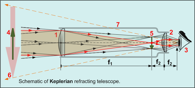


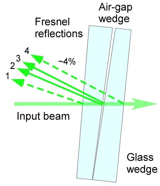
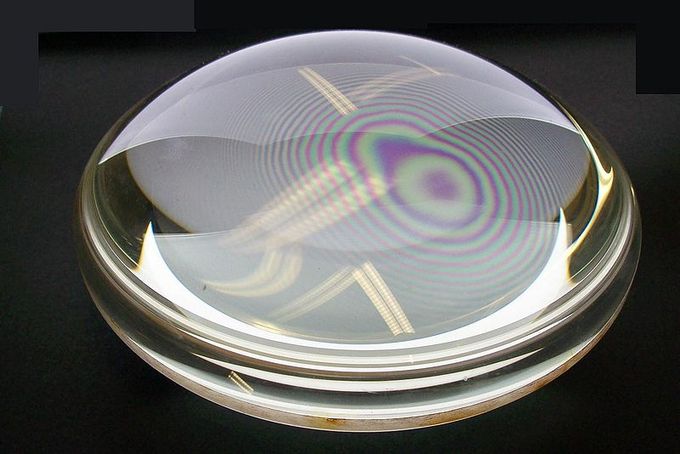

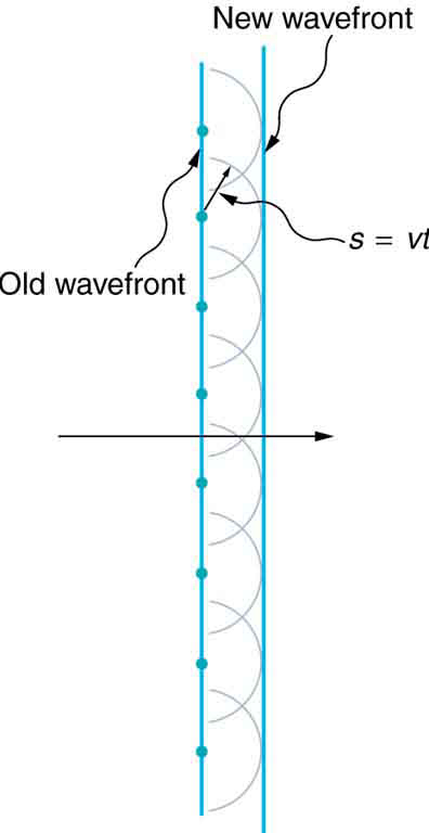
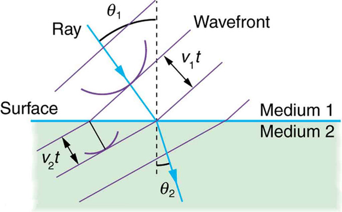
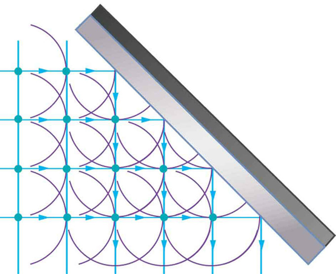
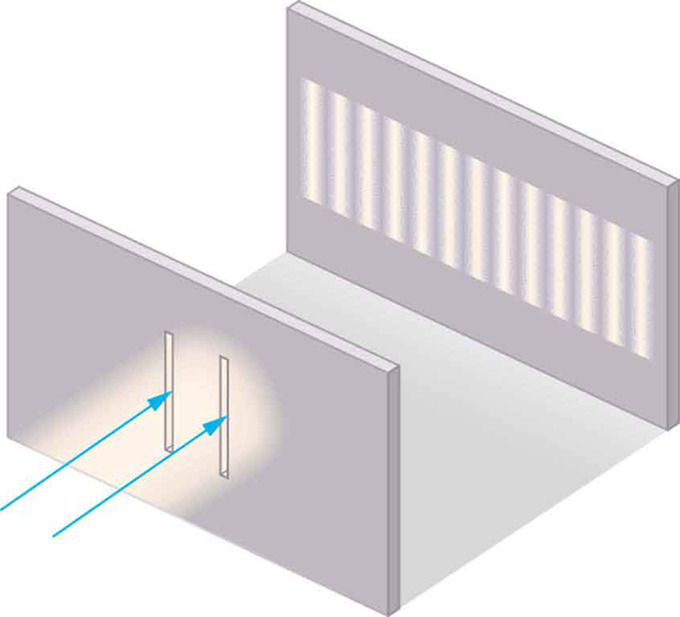
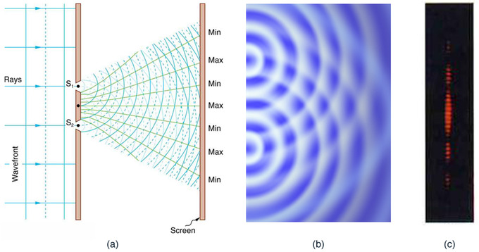
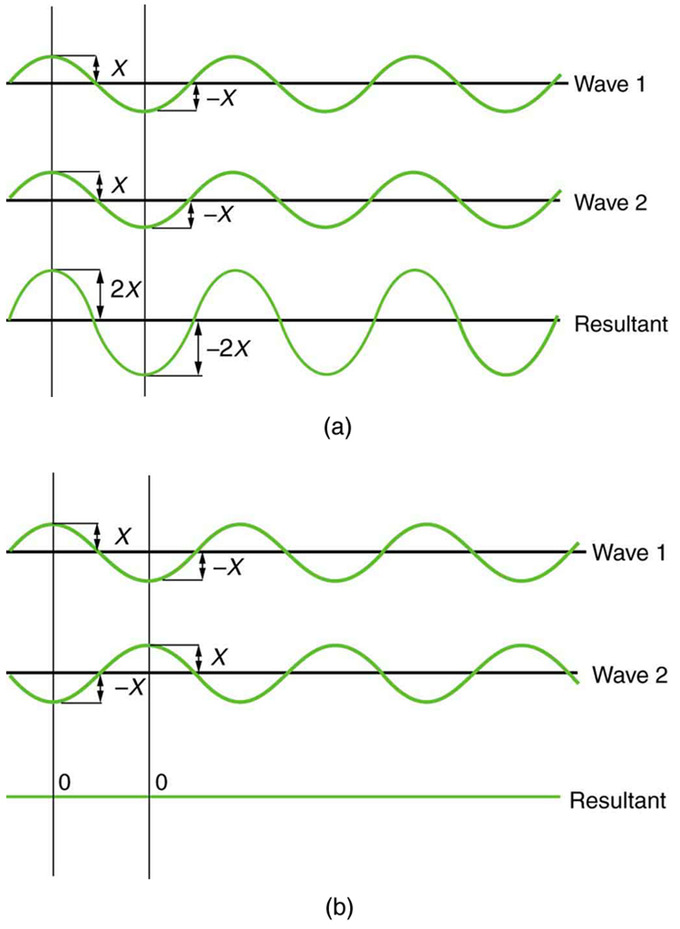

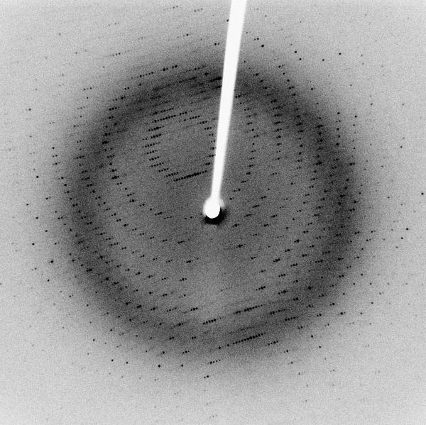
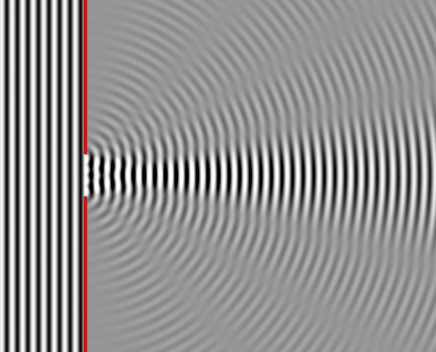
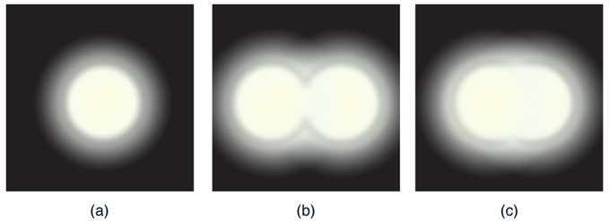
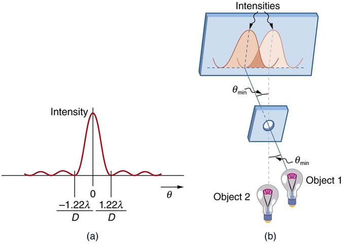

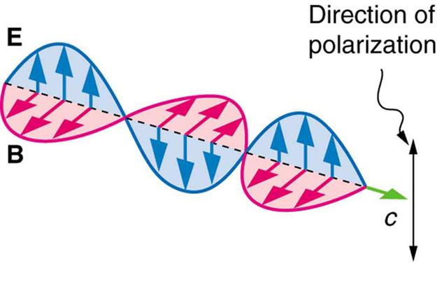

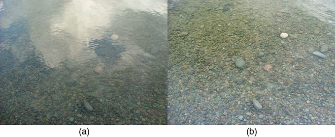
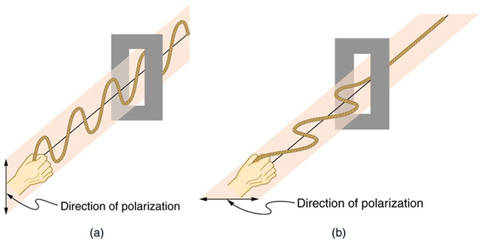
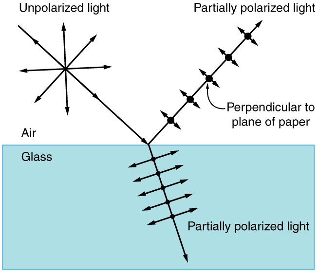
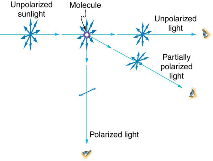


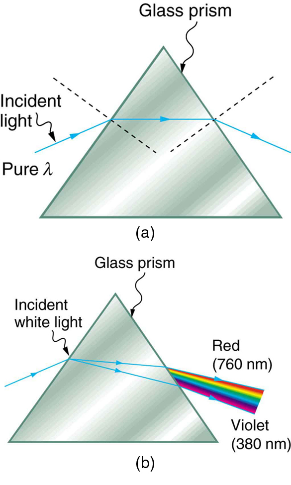
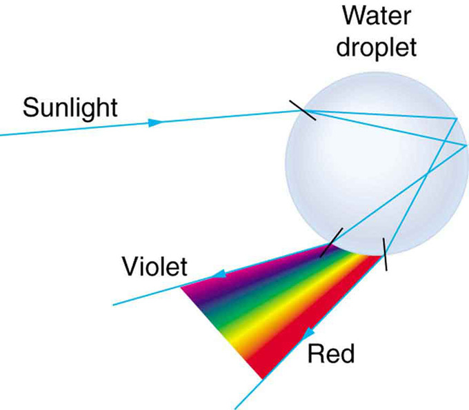


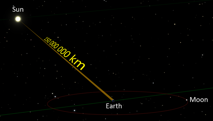


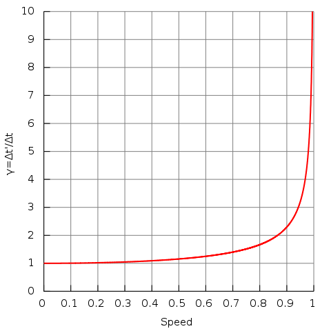


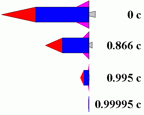
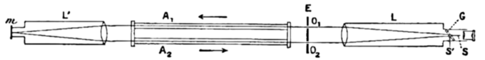
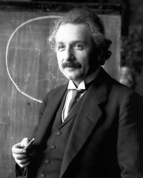


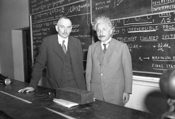
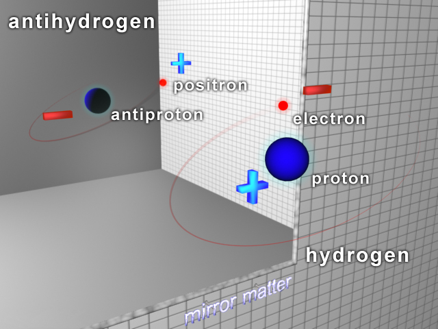
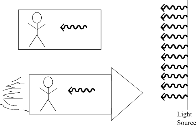

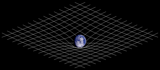
Nice to be visiting your blog again, it has been months for me. Well this article that i’ve been waited for so long. I need this article to complete my assignment in the college, and it has same topic with your article. Thanks, great share. digital microscope
BalasHapus