snow earth and its future go to steady artificial snow so MIT robot swims AMNIMARJESLO BUSAF XAM 0220
Snow And Humans
Times Snow Defeated Humans
Nice Try
"A snow blower and a lawn mower are, like, basically the same thing right? Let me just go mow my driveway real quick."
XXX . V THE FUTURE OF SNOW
The potential for snow to supply human water demand in the present and future Runoff from snowmelt is regarded as a vital water source for people and ecosystems throughout the Northern Hemisphere (NH). Numerous studies point to the threat global warming poses to the timing and magnitude of snow accumulation and melt. But analyses focused on snow supply do not show where changes to snowmelt runoff are likely to present the most pressing adaptation challenges, given sub-annual patterns of human water consumption and water availability from rainfall. We identify the NH basins where present spring and summer snowmelt has the greatest potential to supply the human water demand that would otherwise be unmet by instantaneous rainfall runoff. Using a multi-model ensemble of climate change projections, we find that these basins—which together have a present population of ~2 billion people—are exposed to a 67% risk of decreased snow supply this coming century. Further, in the multi-model mean, 68 basins (with a present population of >300 million people) transition from having sufficient rainfall runoff to meet all present human water demand to having insufficient rainfall runoff. However, internal climate variability creates irreducible uncertainty in the projected future trends in snow resource potential, with about 90% of snow-sensitive basins showing potential for either increases or decreases over the near-term decades. Our results emphasize the importance of snow for fulfilling human water demand in many NH basins, and highlight the need to account for the full range of internal climate variability in developing robust climate risk management decisions.
Introduction
The accumulation of snow is a vital source of water for natural systems and humans (Barnett et al2005, Westerling et al2006, Viviroli et al2007, Kurz et al2008, Rood et al2008, Pierson et al2013). For humans, snow is a crucial natural reservoir (Barnett et al2005), providing both flood control and water storage by capturing water in solid form in cold months and releasing it in warm months, concurrent with higher agricultural and evapotranspirative demands (Hayhoe et al2004, Viviroli et al2007, Barnett et al2008). Snow can also serve as a sentinel system, providing a benchmark by which the advance of global warming can be measured (Barnett et al2008, Renard et al2008).
Yet analyses reveal that the relationship between snow and warming is more complex than monotonic declines, particularly given that trend detection in mountainous regions is challenging (Brown and Mote 2009, Viviroli et al2011). In the Western US, for example, increases in freezing elevations (Ashfaq et al2013), decreases in snowfall-to-rainfall ratios (Knowles et al2006), earlier snowmelt runoff (Rauscher et al2008), and decreases in snowfall (Pederson et al2013), have been observed together with long-term increases in snow accumulation (Howat and Tulaczyk 2005, Mote 2006, Kapnick and Hall 2010). Further, despite projected snow declines by the end of the century (Diffenbaugh et al2012), the magnitude of internal climate variability suggests that some Northern Hemisphere (NH) regions may experience increases in both mean (Mankin and Diffenbaugh 2015) and extreme (O'Gorman 2014) snowfall for at least the next half century or more, complicating decisions around new water infrastructure or flood management. The implications of a varied snow response for humans and ecosystems will therefore be a function of both the undetermined mix of human-induced climate change and natural climate variability, and the present importance of snow in basin-scale hydrology.
While a number of studies demonstrate that snow supply is vital and likely to decline by mid-century (Barnett et al2005, Rauscher et al2008, Diffenbaugh et al2012, Ashfaq et al2013, Mankin and Diffenbaugh 2015), assessments of snow as a source of water supply are largely inferred from supply-side measures such as the ratio of total annual snowfall to runoff (Barnett et al2005), or the fraction of annual streamflow pulsed in the warm season (Stewart et al2004). Analyses of present snow supply are helpful for identifying the spatial pattern of snow's importance in the overall hydrological cycle (Barnett et al2005, 2008, Viviroli et al2007). However, global warming will not influence the supply of snow or the timing or magnitude of snowmelt runoff equally for all basins (Rauscher et al2008, Adam et al2009, Brown and Mote 2009, Viviroli et al2011, Ashfaq et al2013). Because we do not know snow's relative importance to each region's water supply portfolio, we also do not know the differential risks this heterogeneous response presents to regional water availability in snow-dominated regions.
Human water demand, which is shaped by both basin-scale hydroclimate and the water-demanding activities of people, is supplied by groundwater and surface and subsurface runoff from both rainfall and snowmelt. Given the NH distributions of human water demand, where does snowmelt runoff have the potential to be critical for water supply? Here we present a quantification of the potential for observed and projected snowmelt runoff to fulfill NH spring and summer human water demand. In calculating this 'snow resource potential,' we reconcile the timing and magnitude of each basin's unique sub-annual patterns of snowmelt and rainfall runoff, as well as 'human blue water demand' (surface and groundwater consumption, (Hoekstra et al2012)). We focus explicitly on human demand, noting that ecosystems also place important and varied demands on snow accumulation and melt (Westerling et al2006, Rood et al2008, Pierson et al2013, Tague and Peng 2013), and are also highly exposed to changes in snow hydrology (Westerling et al2006, Kurz et al2008, Rood et al2008, Pierson et al2013).
Methods
We perform our analysis at the basin scale. We focus on identifying those basins likely to be most sensitive to changes in snowmelt runoff, given both the magnitude of human blue water demand (hereafter 'demand'), and the potential for snow to supply the fraction of demand that would otherwise be unfulfilled by instantaneous rainfall runoff. We partition mean basin-scale total runoff (surface and subsurface) into contributions from snowmelt and rainfall (supplementary material), and remove the amount of monthly demand that could be fulfilled by rainfall runoff, as discussed below. The remaining demand is 'unmet', and needs to be supplied by alternative sources, such as from groundwater, surface reservoirs, and/or snowmelt. We then calculate the percentage of cumulative spring and summer unmet demand that could be supplied by cumulative spring and summer snowmelt runoff, which we call the 'snow resource potential'. This snow resource potential will exceed 100% if snowmelt runoff exceeds unmet demand. This partitioning separates those basins where spring and summer rains are theoretically sufficient for human needs, versus those where snow contributions could play a critical role in supplying water in both the present and future climates.
We calculate monthly snowmelt runoff (mm) at the grid-point scale. We use the human blue water footprint (Hoekstra and Mekonnen 2012) to estimate NH basin-scale dependence on snow as a water resource. The blue water footprint refers to human surface and subsurface water consumption across industrial, domestic, and agricultural uses, and was estimated for 1996–2005 at 5 arc minute-resolution (Hoekstra and Mekonnen 2012). We calculate the basin-scale area-weighted blue water footprint (mm/month) minus the historical mean (1955–2005) monthly rainfall runoff (mm/month) to calculate the human water demand that remains in a given month. When remaining demand is a positive amount, we term this remaining blue water footprint 'unmet demand'.
To estimate the potential for NH snowmelt runoff to supply basin-scale unmet demand, we calculate the ratio between the cumulative boreal spring and summer (March–August) snowmelt runoff and cumulative unmet demand (figure 1). When expressed as a percentage, we call this measure the 'snow resource potential'.
Figure 1. Snow resource potential in the present climate. (a)–(d) 1955–2005 March through February cumulative unmet demand (UD), orange, and snowmelt runoff (snmQ), light blue, both referenced to the right axis (mm) and their ratio (snmQ/UD), dark blue, referenced to the left axis (snmQ/UD), for example basins: the San Joaquin (a), Colorado (b), Syr Darya (c) and Indus (d). In each panel, August is highlighted in red to show the value plotted in (e), which is the August snmQ/UD cumulative ratio multiplied by 100, or what we term, the 'snow resource potential'. (e) The snow resource potential. Blue-stripped regions indicate basins for which instantaneous monthly rainfall runoff is sufficient to meet all March–August basin-scale demand. White regions have no snowmelt runoff.
We estimate March–August rainfall runoff, snowmelt runoff, unmet demand, and snow resource potential for the 'historical' (1955–2005) and 'future' (2006–2080) periods in reanalysis (historical) and in transient climate simulations (historical and future). For the historical period, we rely on version 2 of the Global Land Data Assimilation System (GLDAS)—a 0.25° gridded reanalysis of surface land variables—to provide estimates of observed land surface processes (Rodell et al2004). The estimates from this dataset provide an observed climatological baseline against which to evaluate projected future changes.
We use two global climate model ensembles forced in the IPCC AR5 RCP8.5 emissions pathway (Riahi et al2011) to simulate both historical and future snowmelt runoff and rainfall runoff (supplementary material). RCP8.5 provides the emissions pathway most similar to observations since 2005 (Peters et al2013). We use these two ensembles forced in RCP8.5 to capture several different sources of uncertainty in the projections of future climate. The first is the Coupled Model Intercomparison Project (CMIP5) (Taylor et al2012), which includes GCMs that simulate coupled interactions among the atmosphere, ocean, land, and sea ice at varying resolutions (Taylor et al2012, Flato et al2013). We use one run from the 19 CMIP5 models that provide the requisite output fields providing a 19-member CMIP5 ensemble (table S1). The second ensemble is NCAR's single-model 'large ensemble' (LENS), which consists of 30 simulations of the Community Earth System Model (CESM) (Kay et al2015). CESM is a coupled atmosphere–ocean–land–sea-ice model that simulates climate at 1° × 1° atmospheric resolution. LENS encompasses 30 simulations of the climate from 1920 to 2080, using both observed and projected (RCP8.5) forcing. Each LENS member is initialized with the same ocean and sea-ice conditions, with the only difference being small perturbations to the initial atmospheric state.
In analyzing both CMIP5 and LENS in a single forcing pathway, our estimations of risk of future declines in the snow resource potential come from two sources of ensemble uncertainty. CMIP5 provides a range from an undetermined combination of model structure and internal variability, while the LENS provides an estimate of 'irreducible' uncertainty from CESM's representation of internal climate variability (Deser et al2012a, 2012b, Kay et al2015, Mankin and Diffenbaugh 2015). Internal variability exerts a large influence on long-term hydroclimate and snow accumulation (Rauscher et al2008, Kapnick and Delworth 2013, Mankin and Diffenbaugh 2015), which can create an irreducible range of uncertainty on multi-decadal time scales.
We convert all gridded data to mm/month and compute area-weighted averages for basins demarcated by a modified version of the Simulated Topological Network 30p (STN-30p) (Vörösmarty et al2000). STN-30p is a 0.5° resolution dataset representing the spatial extent of drainage basins. We modify STN-30p using the coastal basins of (Meybeck et al2006) to aggregate small coastline basins into larger basins following the methods of (Viviroli et al2007). We analyze basins with centroids >10 °N latitude, and mask small basins for which the GLDAS 0.25 data are too coarse, providing 421 NH basins for our analysis. Gridded human population estimates for 2015 are retrieved from the Center for International Earth Science Information Network (CIESIN, FAO & CIAT 2005).
We calculate basin-scale monthly-mean linear trends in snowmelt runoff and rainfall runoff from 2006 to 2080 in each of the CMIP5 and LENS realizations, yielding time trend coefficients based on the 75 year basin-scale time series. We express each simulation's linear time trend relative to its respective historical (1955–2005) monthly mean climatology. We present these time trends as percent change per 50 years. To account for biases in the CMIP5 and LENS simulations, we project these relative changes in snowmelt runoff and rainfall runoff onto the GLDAS historical monthly mean climatology. We multiply each realization's monthly relative trend (fraction of that realization's historical mean) by the GLDAS monthly value. We add this relative change to the GLDAS baseline monthly mean, providing 49 estimates of absolute change (19 CMIP5, 30 LENS) in future monthly snowmelt runoff and rainfall runoff in each basin. We then estimate the future unmet demand and snow resource potential for each realization, and difference it from the GLDAS-based observational baseline. This method is similar to the statistical change factor method used to downscale climate data (Minville et al2008, Chen et al2011); however, rather than projecting onto daily-scale observations, we add the relative changes in the future monthly means to observed monthly means. Following the IPCC (Collins et al2014, Diffenbaugh et al2014), risks are calculated as the percent of the ensemble that agrees on the direction of change.
Results
We show the basin-scale evolution of spring and summer snowmelt runoff and unmet demand for the San Joaquin, Colorado, Syr Darya, and Indus basins (figures 1(a)–(d)). The observed seasonal relationship between snowmelt runoff and unmet demand is basin-dependent. For instance, in the agriculturally intensive San Joaquin, unmet demand begins to accumulate in May as snowmelt runoff slows. The mismatch in runoff timing suggests the importance of storage reservoirs to supplying water during the dry season, which is also when agricultural demand, and thus unmet demand, is highest. By August, the snow resource potential is ~17% of unmet demand. In contrast, in the Indus basin, where the sub-annual evolution of human water demand and rainfall runoff is quite different than the San Joaquin, the August snow resource potential is ~180%.
Snowmelt runoff is a spatially dominant feature of the NH spring and summer hydrological regime: 305 of the 421 basins have March–August snowmelt runoff. Yet despite snowmelt runoff's ubiquity, more than two-thirds of NH basins (280 of 421) have sufficient spring and summer rainfall runoff to meet all spring and summer human demand (figure 1(e)). Of these 421 basins, we identify 97 snow-sensitive basins (i.e., basins with both climatological spring–summer snowmelt runoff and unmet demand). These basins are presently home to ~1.9 billion people. The snow-sensitive basins are geographically limited to approximately 25–45 °N (near the sub-tropical high pressure centers) (figure 1(e)). Notable exceptions are the extremely high latitudes, where human populations are low and all human water demand can be met by runoff from snowmelt.
For many snow-sensitive basins, spring–summer snowmelt runoff exceeds unmet demand many times over, meaning that even large decreases in snow supply may not pose risks for human water consumption. However, at least 46 basins have snowmelt runoff fulfilling unmet demand. These 46 basins are currently home to 1.5 billion people. For example, in the Ganges–Brahmaputra, where 700 million people live, ~76% of unmet demand can be supplied by snowmelt runoff. In the Shatt al-Arab basin that spans much of the Middle East, the snow that accumulates in the Zagros Mountains can supply ~56% of the spring and summer total unmet demand for its ~67 million people.
Using the LENS and the CMIP5 model projections, we examine the risks of increases in unmet demand and decreases in snow resource potential (figures 2(a) and (b)). Decreases in spring and summer rains pose the risk that some basins that currently have enough rainfall to meet human water demand (hatched basins in figure 1(e)) may transition to having unmet demand by 2060 (gray basins in figures 2(a) and (b)), even without considering possible future increases in human demand. In the CMIP5 ensemble-mean, 68 basins (with >319 million people) transition from sufficient to insufficient instantaneous rainfall runoff for human consumption, including the Mississippi basin in central North America. In LENS, 31 basins (totaling ~100 million people presently) transition to having net unmet demand profiles in the future (figure 2(b)).
Figure 2. Risks of decreased March–August snowmelt supply and increased unmet demand by 2006–2080. For the CMIP5 (left column, (a), (c)) and the LENS (right column, (b), (d)), we show the risks of decreases in snowmelt resource potential in (a), (b). Basins with blue lines indicate basins for which future rainfall runoff is sufficient to meet present human water demands. (c), (d) Basins with joint risks for both snowmelt decreases and unmet demand increases. Gray basins in (a) and (b) indicate basins that shift from sufficient to insufficient rainfall runoff to meet water demand in the ensemble-mean. These basins are projected to be snowmelt dependent. Their ensemble-mean snow resource potential projections are shown in figure S1.
The 97-basin mean risk of decreased snow resource potential is greater than 60%: it is 67% for CMIP5, and 64% for LENS. A decrease in the snow resource potential is governed by a combination of sub-annual changes in rainfall runoff (which can change the spring and summer unmet demand profile), and by changes in the magnitude and timing of snowmelt. We therefore calculate the joint risk of combined decreases in snowmelt runoff and increases in unmet demand (figures 2(c) and (d)). In CMIP5, 20 basins (with ~27 million people) exhibit >50% risk of both increased unmet demand and decreased snowmelt runoff, while in LENS, 6 basins (with >10 million people) have >50% risk (figures 2(c) and (d)) by 2060.
While the risk of decreasing snow resource potential is large in many basins (figure 2), there is substantial uncertainty in the fraction of unmet demand that is likely to be met by snowmelt runoff by 2060 (denoted by basin stippling in figures S1(b) and (c), which shows the CMIP5 and LENS ensemble mean projections). Indeed, for both the multi-model CMIP5 ensemble and the single-model LENS ensemble, the majority (~90%) of snow-dependent basins span positive and negative changes in the snow resource potential (figures 3(a)–(f)). Only three basins show declines across all realizations in both ensembles, all three of which exhibit low snow volumes in the baseline climate: on the Iberian and Italian peninsulas (the Duero-Adour and Central Apennines respectively), and in the Rio Grande basin spanning Texas and Mexico. The lack of unequivocal robustness in both the CMIP5 and LENS ensemble-mean responses highlights the large variations in the long-term future snow resource potential. In particular, the fact that the single-model LENS ensemble does not simulate a consistent sign of change in a number of basins suggests that much of the uncertainty in future snow resource potential can arise from internal variability.
Figure 3. Ensemble range in snow resource potential change at 2060. For each ensemble, CMIP5 (left column, (a), (c), (e)) and the LENS (right column, (b), (d), (f)) we show the full ensemble range in the change of future snowmelt supply potential differenced from the present potential, expressed as percentage points: the basin minimum (a), (b), the ensemble mean (c), (d), and the basin maximum. (e), (f) Gray basins are those for which future rainfall runoff is insufficient to meet human water demand. Stippled basins in (c), (d) indicate basins for which the ensemble-mean trend is less than 1 SD of the ensemble variability.
To quantify the potential basin-scale interactions of rainfall and snowmelt runoff in determining future snow resource potential, we calculate the seasonal average (March–August) ensemble-mean trends in snowmelt and rainfall runoff in CMIP5 and LENS (figure 4). For snowmelt runoff, the ensembles show similar patterns of high-latitude increases and mid-latitude decreases (figures 4(a) and (b)). Along with projected increases in warm-season precipitation, there is an increase in spring and summer rainfall runoff in the high and mid-latitudes (figures 4(c) and (d)). For most basins, decreases in snowmelt runoff are associated with increases in rainfall runoff, suggesting that at least some of the decrease in snowmelt runoff results from a transition of precipitation from snowfall to rainfall. The exception is a collection of basins in Central America, the Mediterranean, and Central Asia that exhibit declines in both snowmelt and rainfall runoff. Like the ensemble-mean changes in the snow resource potential, there are large uncertainties in the magnitude of the ensemble-mean trends in rainfall and snowmelt runoff, indicated by the vast stippled areas in figure 4. For both rainfall runoff and snowmelt runoff, the variability in the seasonal trends within LENS spans a large percentage of the CMIP5 variability, including many of the snow-sensitive basins identified in our analysis, particularly around the Western US and the Mediterranean (figures 4(e) and (f)). As with the snow resource potential, the fact that the LENS range spans a large fraction of the CMIP5 range suggests that much of the multi-model uncertainty could arise from internal climate variability.
Figure 4. Ensemble-mean trends from CMIP5 and LENS. (a), (b) March–August ensemble-mean linear snowmelt runoff trends, estimated from 2006 to 2080 in the CMIP5 (a) and LENS (b), expressed as percent change per 50 years. (c), (d) As in (a) and (b) but for rainfall runoff. (e), (f) The percent of the variability in CMIP5 trends in snowmelt runoff (e) and rainfall runoff (f), spanned by the LENS ensemble. Stippled basins in (a)–(d) indicate basins for which the ensemble-mean trend is less than 1 SD of the ensemble variability.
To identify the basins that are most likely to be sensitive to snow supply changes, we highlight key results for basins that meet the following criteria: (1) basins with a March–August snow resource potential of 1–250% in the observed historical baseline, and (2) a present population of over 1 million people. Together, these criteria focus our analysis on large or population-dense basins. In particular, the 1–250% inclusion criterion emphasizes places where snowmelt runoff has a non-zero potential to supply unmet demand but does not exceed unmet demand so many times over that the basin is potentially insensitive to changes in snowmelt or rainfall runoff.
We find that 32 basins, encompassing ~1.45 billion people, meet these criteria (table 1, map inset). Particularly sensitive basins include the Kizil Irmak (basin ID 14), Asi (basin ID 15), Asksu (basin ID 16), and Aegean (basin ID 11) in the Mediterranean region, and the Ebro-Duero (basin ID 9) on the Iberian Peninsula. These five regions show 100% risks of declining snow resource potential across the 19 CMIP5 models. In contrast, the highly populous Indus river basin (~270 million) has lower risks of decreased snow resource potential, in part due to modest increases in rainfall runoff projected in LENS, and modest but uncertain increases in snowmelt runoff in the CMIP5.
Table 1. Risk profiles of snow sensitive basins. We show the 32 snow sensitive basins that meet the following criteria: (1) observed late 20th century snowmelt runoff is 1—250% of unmet demand, making it sensitive to changes in water supply and (2) more than 1 million inhabitants. For these 32 basins, totaling 1.45 billion people, we show the observed snowmelt dependency, the risk of decreases in this measure in both the CMIP5 and LENS ensembles. Outlined in red are the four additional basins that do not meet the 1 M inhabitant threshold, but have population densities >5 people/km2: [a] Klamath Basin (snmQ/UD: 125%; CMIP risk: 79%; LENS risk: 93%); [b] Western Great Basin (snmQ/UD: 239%; CMIP risk: 74%; LENS risk: 33%); [c] North Black Sea-Crimea (snmQ/UD: 2%; CMIP risk: 94%; LENS risk: 100%); and [d] Western Dzungarian (snmQ/UD: 95%; CMIP risk: 47%; LENS risk: 73%).
#
Name
Population (mil.)
snmQ/UD index (%)
CMIP Risk (%)
LENS Risk (%)
1
Sacramento
4.93
25
95
87
2
Coastal California
3.73
2
89
73
3
San Joaquin
6.30
17
95
90
4
Colorado (South)
1.21
1
74
50
5
Upper Great Basin
2.44
46
63
50
6
Colorado
9.65
207
74
50
7
Rio Grande
16.46
114
95
100
8
Atlas
25.48
2
95
100
9
Ebro-Duero
32.20
10
100
100
10
South Apennines
1.13
3
95
97
11
Aegean
12.14
35
100
97
12
Buyuk Menderes
9.74
8
95
100
13
Sakarya
1.29
179
95
70
14
Kizil Irmak
6.38
24
100
80
15
Asi
19.19
15
100
97
16
Aksu
1.97
151
100
90
17
Dead Sea
15.71
1
84
77
18
Shatt al Arab
67.44
56
95
73
19
Urmia
5.25
26
68
57
20
South Caspian
8.41
18
95
67
21
Masileh
21.23
16
79
70
22
Karun
13.85
1
79
70
23
Garagum
9.68
3
79
73
24
Farah
12.74
164
79
70
25
Syr Darya
27.14
50
58
60
26
Ili
4.46
34
47
50
27
Alakol
1.72
44
53
47
28
Dzungarian
10.74
16
53
73
29
Upper Ili
1.11
2
68
67
30
Indus
269.43
105
37
33
31
Ganges
696.82
77
63
47
32
Huai
131.59
1
58
37
Discussion
Our measure of snow resource potential is defined by two requisite factors: that NH spring and summer snowmelt runoff is a climatological feature of the hydrological basin, and that human water consumption exceeds water available from instantaneous rainfall runoff. This formulation allows us to focus explicitly on the potential of the snow resource to supply human water demand that is not met by rainfall. However, because snow is not the only source of water storage for humans, and because snow is also critical for fulfilling water demanded by ecosystems, a number of caveats beyond the assumption of the RCP8.5 scenario must be considered.
First is that our measure does not consider the needs of each basin's environmental runoff requirements, nor how changes in snowmelt timing will affect ecosystems and their required nutrient loadings (Pierson et al2013). Warmer temperatures imply greater potential evapotranspiration and probable changes in soil moisture during the dry season (Seneviratne et al2010). Further, a snow-to-rain phase change could potentially decrease streamflow (Berghuijs et al2014), suggesting the possibility of net runoff decreases in warming basins irrespective of precipitation changes. Neither the ecological contributions to total water demand nor the ecological consequences of these shifts in basin hydrology are captured in our analysis.
Second is our treatment of the human dimension. Total human population—and thereby total water demand—will almost certainly increase in the future. However, we do not predict changes in total population or the geographic distribution of people, nor the changes in consumption patterns that are likely to accompany future socioeconomic changes. To do so would introduce additional sources of uncertainty, whereas our aim is to isolate the uncertainty from climate change. The likelihood that population growth and economic development increase human water demand in the future implies that our analysis provides a lower bound on the risks that global warming will present to snow resource potential, as increasing population and/or per capita consumption will further increase the total amount of water required to meet human demand.
Third is that our measure of snow resource potential quantifies the size of the snow water resource given climatological factors and present human water demand, but does not consider whether basin-scale water availability is sustainably managed. The basins that we identify as being sensitive to snow changes, for example, may have sufficient surface storage infrastructure or groundwater resources to ensure water supply during months of shortfall, rendering snowmelt runoff less critical for meeting unmet demand. Conversely, a number of rainfall-sufficient basins (hatched regions in figures 1–3) may be reliant on the extra volume of water provided by snowmelt runoff for hydropower or other managed systems (Rauscher et al2008), or may not be positioned to collect and store all the rainfall runoff within the basin. Furthermore, our analysis of the most sensitive basins includes a minimum population criterion of 1 million people (table 1). It is possible that adjacent basins with smaller populations could together represent areas of equivalent exposure when considered together as a contiguous unit. If basin-scale population densities of at least 5 people per km2 are considered rather than population totals, four additional basins meet the inclusion criteria presented in table 1.
It should be noted that the assumption of the RCP8.5 pathway, which is the highest available in the AR5, could influence not just the risks of decreased snow resource potential for basins, but also the relative magnitudes of the basin-scale uncertainties between the CMIP5 and LENS. Presumably, the expression of internal variability in both ensembles will represent an increasing fraction of total uncertainty under lower emissions trajectories. How this will change the relative magnitudes of uncertainty between the CMIP5 and a LENS-like experiment requires further testing.
Fourth, there are several spatial and temporal factors that influence our analysis, and therefore our results. Because we consider the size of the snowmelt resource over a 6-month window (March–August), the temporal scale we consider is too coarse to identify subtler, but potentially critical, shifts in snowmelt runoff peaks that change dry season lengths (Rauscher et al2008, Ashfaq et al2013). There are also considerable sub-basin heterogeneities (such as from topography or soil heterogeneity) that can influence the timing and magnitude of observed water availability at smaller temporal scales (Rauscher et al2008, Adam et al2009). The scale at which snow and snowmelt runoff are resolved in models is also a critical limitation (Rauscher et al2008, Pavelsky et al2012, Ashfaq et al2013). The CMIP5 ensemble has divergent estimates of snow accumulation (Diffenbaugh et al2012). Sources of model divergence in estimates of snow include (1) simulations of synoptic-scale atmospheric processes that create snowfall, model representations of topography (Mote 2006), and fine-scale processes that are parameterized at sub-grid-scales in the models, such as snow albedo and cloud feedbacks (Qu and Hall 2006, 2014). Such limitations influence model bias and therefore, ensemble-mean bias. This is a justification for examining the full distribution of snow-related changes produced by the both the CMIP5 and LENS and comparing their relative spans as in figure 4. However, it should be emphasized that neither ensemble explicitly resolves all of the processes that create snowfall and snowmelt.
The different means by which models treat these snow-related processes is often cited as the reason for the large multi-model uncertainty in CMIP5 (Rauscher et al2008, Ashfaq et al2013). However, our results suggest that irreducible uncertainty from model representations of internal variability at coarse spatial scales can span a similarly large uncertainty (figures 4(e) and (f)). It is important to note that the similar range of uncertainty in future snowmelt in the LENS and CMIP5 in some basins may not hold for simulations at finer scales that better resolve the atmosphere and land surface (Rauscher et al2008). In higher resolution simulations, the magnitude of warming appears to be sufficiently large to overwhelm fine-scale precipitation variability arising from complex topography (Ashfaq et al2013). It remains, however, that the large uncertainties within the single-model LENS ensemble highlight the potential for internal variability to exert a large influence on monthly-scale hydroclimate, and therefore risks of declines in snow resource potential. Furthermore, the magnitude of the LENS uncertainty suggests the possibility that, for some climate impacts, the fraction of total CMIP5 ensemble uncertainty contributed by internal variability may be larger than the fraction contributed by model differences.
Conclusions
Our estimate of snow resource potential provides a meaningful baseline for quantifying the risk that different regions face from changes in climate (such as from global warming or internal climate variability) and/or changes in demand (from population or land-use change). It can also be reconciled against analyses of basin-scale vulnerability and adaptation capacity (World Water Assessment Programme 2009).
We conclude that, should greenhouse gas emissions continue along their recent trajectory, which is at or above the RCP8.5 scenario analyzed here (Peters et al2013), the risks of declines in snow resource potential exceed 67% in snow-sensitive basins, potentially impacting spring and summer water availability for nearly 2 billion people. In the CMIP5 ensemble-mean, global warming also shifts an additional 68 basins to have spring and summer rainfall runoff that is insufficient to meet human water demand, even without accounting for increases in demand that are likely to arise from population growth and economic development. These basins are particularly critical, as emerging increases in unmet demand must be supplied by alternative sources, in many cases within the context of decreasing snow resource potential.
Our results highlight the basins where future snow changes pose the greatest risk to people's present water demand patterns. We present these risks in the context of climate uncertainty, including the irreducible uncertainty from internal climate variability. Given present demand, this irreducible range is sufficient to create ambiguity in the sign of decadal trends in future snow resource potential. A number of other uncertainties exist in future water resources from snow, many of which reside in the human dimension, including where and how people manage and respond to water resources in a changing climate. Our results provide critical context for climate risk management (Milly et al2008, Kunreuther et al2013) and robust adaptation decisions (Lempert and Collins 2007, Milly et al2008, Kunreuther et al2013) that require identification of critically snow-dependent basins and quantification of irreducible uncertainty in future climate trajectory.
XXX . V00 Climate change: past and future
Climate change, past and future warming
Evidence from fossils, ice cores and weather recordings in Antarctica
Watch a video showing the extraction of an ice core
The evidence in ice cores
The beauty of ice cores is that they contain a variety of forms of evidence that can tell us so many different things about the past climate and environment. The evidence is also continuous through time and can be dated with a high degree of precision. Some important types of evidence and information are:
Stable isotope ratios of the oxygen and hydrogen making up layers of ice are used to reconstruct the air temperature at the time that the snow fell.
Where annual layers of ice can be identified, the thickness of layers indicates the yearly quantity of snowfall in the past.
The concentration of dust preserved in layers of ice gives an indication of how much wind erosion was occurring on continents in the past (related to both the strength of winds and the levels of vegetation cover over the land in the past).
Tephra shards and levels of acidity of the ice show when major volcanic eruptions happened in the past.
Air trapped inside the ice can be analysed for its concentration of carbon dioxide and methane, indicating how concentrations of these greenhouse gases in the atmosphere have fluctuated through time.
A slice of an ice core showing trapped air bubbles
XXX . V0000 Urban water future: Changing climate means changing water
The T.W. Daniel Experimental Forest, located about an hour up Logan Canyon from Utah State University, is full of all kinds of shiny metal objects.
The metal feathers of rain gauge windscreens rattle with the breeze. Mylar insulation wraps trees, which helps measure sap flux and how conifers transpire water. All kinds of sensors and instruments measure soil moisture, snow water equivalent and weather, then transmit the data down to the valley below.
The majority of Scott Jones’s instruments are kept in a small plot, around 200 by 400 yards, but they’re adding to the volume of information helping scientists build better climate models. Those models, in turn, will help water managers have a better idea of what to plan for with a changing climate.
“We’ve seen a lot of rain this year, which is unusual,” Jones said, who works as a professor of environmental soil physics at Utah State. “So that’s one of the questions we’re interested in … what’s going on with the transition between where it’s raining and where it’s snowing? That can be a big factor in the water that’s delivered to the reservoirs.”
It was a weird and warm winter in northern Utah. By mid-March, the T.W. Daniel Experimental Forest was still only accessible by snowmobile, but snowpack sat at only 75 percent of normal.
A big water shift is coming to the West, and both researchers and policymakers want to know what it means for Utah. Jones’s research at the Experimental Forest is part of iUTAH, or “innovative Urban Transitions and Aridregion Hydro-sustainability, a five-year collaboration among universities, government and other interested parties to monitor water on a large scale in the state. Sites are set up on Red Butte Creek in Salt Lake, the Provo River in the Heber Valley and on the Logan River.
As it turns out, looking at things as small and localized as the soil, snow and trees on a tiny plot in Logan Canyon helps researchers understand a lot about our region’s water and the larger global climate system.
Back at the university, situated at the mouth of the canyon just above the Logan River, researchers at the Climate Center are using this site-specific data to fine-tune climate models and make forecasts about future water supplies. They’re also on a mission to educate the public and policymakers, providing clarity in a torrent of information about climate change.
“The trend is definitely upward in terms of coming to grips with the notion that the climate is changing and humans are driving that change,” said Robert Davies, an extension climatologist at the Climate Center. “Within the state of Utah, there are many, many people who accept it; certainly Utah’s scientific community does en masse.”
Before he can explain the future implications of climate change on northern Utah’s water supply, Davies said it’s important to first wrap one’s head around the complexities at play — what researchers know, what they don’t know and why that’s important.
“It’s important because the science has profound implications for public policy,” he said. “There’s so much conflicting information from the media … Let’s just say that if you’re confused about it, you have every right to be.” Ebbs, flows and tides
Davies said that when most people think about the word “climate,” they associate the term with “average weather.” But when scientists talk about climate change, they’re really talking about two kinds of change, in variability and trend.
Davies compares the two changes to standing on a beach, watching the ocean.
“As the waves come in, some come higher than others, and that’s the variability in the water level in the short-term,” he said. “Contrast that with a trend, which is the tide coming in, and that happens over a longer period.”
An observer on the beach experiences both waves and tides at the same time. The trick is sorting out the two.
“They have different mechanisms, and different things that cause them,” Davies said. “From a climate science perspective, you’re trying to untangle what’s happening in the climate is as of the variability, or a natural oscillation of the climate cycle, and what’s part of the trend.”
Scientists have a good grasp of the tide, or trend. It’s global warming, caused by a build-up of greenhouse gasses that doesn’t let energy escape the planet, leading to an overall warming of the planet. Figuring out what’s behind the variability of climate change is trickier. Scientists are still sorting out the waves from the tide from their location on the shore.
“Variability has to do with how the Earth’s system redistributes energy,” Davies said. “So energy comes in from the sun, it gets warmer in the tropics than at the poles, and the Earth’s system redistributes that energy.”
A big part of that redistribution comes from currents and circulations in the atmosphere. Another big piece of energy distribution comes from the ocean, and those cycles all operate on different time scales.
“With the atmosphere, it’s hours to weeks,” Davies said. “With the oceans, it’s more like once in a millennium.”
Between those cycles, there are other cycles that interact and happen at timescales lasting from decades to centuries.
“What we find is that things happening on a cyclic value in some parts of the world will affect you in other parts of the world,” Davies said. Circulating water
To understand all those interacting cycles and how they influence a small portion of the globe, Davies has another comparison. Utah is like a hole in a golf course, and an atmospheric cycle is like turning on a sprinkler, which moves water in a circle.
“So you’ve got wet cycles and dry cycles, wet and dry,” he said.
More sprinklers turn on, operating at different speeds. Sometimes the sprinklers overlap the hole at the same time, sometimes none are cycling water into the hole as they water other parts of the course. Like the hole on a putting green watered by multiple sprinklers, Utah’s precipitation cycles arise from cycles in the oceans and atmosphere, often thousands of miles away. These “climate oscillations" arise from the redistribution of energy from equator to poles. (Image courtesy Utah Climate Center)
“By studying that over time, you can start to back out and say ‘I think there are three cycles going on,’” Davies said.
By studying these overlapping cycles, scientists can also figure out where the cycles are coming from and how long they take.
“There are different techniques for doing that, and this is a lot of what we do at the climate center, is tying natural cycles to Utah,” Davies said.
He noted three powerful cycles driving the state’s climate, influencing temperatures and the precipitation that fills our mountains, streams and reservoirs. One comes from the Western Pacific, with oscillations in sea surface temperature. Another comes from oscillations in air pressure over the Arctic and another comes from the Atlantic. Climate change, arising from an imbalance of energy entering the Earth system (less energy leaving than entering) can have an effect on cycles, changing their intensity, their duration, even creating new cycles — like changing how quickly the sprinklers rotate, how often they turn on, and how much water flows through them. (Image courtesy Utah Climate Center)
“All of these things happen on different timescales, typically years to decades, but they’re cyclic,” Davies said. “Once you understand the cycle and mechanism by which the change over there affects you over here, you can make quite long-term projections, which we’ve done.” What trees tell us
To boost those projections, climate scientists have also delved into the past. Using tree rings from sites throughout the state, they’ve mapped northern Utah’s climate past, back 1,000 years. The tree rings give scientists a sense of the area’s natural climate variability before human activity started forcing a global warming trend. As determined by tree ring analysis, northern Utah droughts of the 20th century, particularly the late 20th century, are mild in both depth and duration when compared to those of the past 800 years. Periods considered “drought” by 20th century standards are shaded orange. (Courtesy Utah Climate Center)
“Most of this, let’s say before 1900, is natural variability in the precipitation climate of northern Utah prior to significant greenhouse gas impact,” Davies said. “So there’s no real global climate trend going on here, it’s just what happens based on redistribution of Earth’s energy and what it does to precipitation patterns in northern Utah.”
In other words, tree ring records show which sprinklers have been watering our part of the putting green in Utah, and how long it takes them to cycle. The records also show some long periods of drought, in some cases lasting decades. The period including the 20th century, however, has been unusually wet. Dendrochronologist with the U.S. Forest Service Justin DeRose shows off some of the douglas fir and Utah juniper samples they have brought back to study at the dendrochronology workspace at Utah State University on Friday, March 13, 2015. A measuring tape along the edge of the table captures patterns in tree rings to help identify the years of each ring. This information can be used to identify years of excess rain and drought. (Briana Scroggins/Standard-Examiner)
“So here’s the question. Are we on the extreme edge of the this natural variability and we can expect to plop back?” Davies said. “Or is the 20th century wetter because of a changing climate?”
When the Earth’s entire climate system changes, it doesn’t just change the averages in temperature and precipitation, it changes the variability, or extremes, as well.
“This part of the globe, the North American West, and the Western U.S. in particular, turns out to be particularly difficult to make projections for,” Davies said. “What that tells us is we’re missing key features. There are sprinklers out there we don’t know about.” How water will come in northern Utah
Scientists do know the trend. Utah is getting warmer. That means the southern portion of the state will get drier. The variability in northern Utah is a challenge, however. A different set of sprinklers is hitting the area, which means the northern precipitation picture remains unclear.
It might get drier, or it might get wetter. One thing’s clear, however — warmer temperatures mean less water delivered as snow, and more water coming as rain. Warmer temperatures also mean more evaporation, more water in the atmosphere and more intense storm events.
“Here in Logan, we get 30 inches of precipitation a year,” Davies said. “It’s a big difference if we get around three inches every month, or 30 inches in two weeks. It’s still the same amount every year, but how it comes is hugely important.”
For water managers, both the region’s history of drought and our climate future are concerning prospects.
“What it points to is, our need for storage will be greater than it is today,” said Tage Flint, general manager at Weber Basin Water Conservancy District, which operates the seven dams and reservoirs feeding Weber, Davis, Morgan, Summit and parts of Box Elder counties.
Past tree ring data means the region could see long, unprecedented drought, and more water storage will be vital to see Utah residents through. Future climate change means water will no longer be stored in the mountains, as snow, gradually melting off in the summer as consumers need it.
Eric Millis, director of the Division of Water Resources, said climate change in the state also points to a need to look at new water sources.
“I know people beat on the Bear River development and Lake Powell Pipeline, but those two projects bring in water from another basin into Davis, Weber and Salt Lake counties, as well as Washington and Kane counties,” he said. “The projects will help diversify some of the supplies they have.”
Conservation, too, will be key. And if northern Utah does experience the prolonged drought periods shown by old trees, yards and gardens in the region could look very different.
“If we’re just watching the climate get drier and drier, and we have longer droughts than those we experienced in the 20th century, we have no choice but to change landscaping,” Millis said. “We’ve always said we’d adaptively manage, and we hope things will change slowly enough so we can recognize what’s happening and change with it.”
That’s where the models come in. The better scientists understand the cycles and oscillations influencing precipitation in the West, the more planning tools they can provide for water managers.
“We’re trying to get the best models moving forward to plan our supply around,” Flint said. “The extremes of some of those things are outside the realm of our planning, but as we get this new data we try to incorporate it into our water supply options.”
At the T.W. Daniel Experimental Forest, Jones’s research will help further refine those climate models. Mountain landscapes, like Logan Canyon, have a lot of variability compared to flatter terrain. Variability in land surface and vegetation interacts with the atmosphere, and can muddle with human-made models. The more site-specific data researchers gather in Utah, the better our climate models become.
“In terms of questions of climate change, we’re just getting data for that, with this system we have about six years of data,” Jones said. “That’s probably not enough to say a lot about climate change, but certainly, we have seen big changes in precipitation up here.”
But scientists need a long record to get good statistics on climate, and iUTAH funding for the experiment forest study is set to run out in two years.
“Who’s going to continue to fund the maintenance of this hardware? That’s (another) big question we don’t know the answer to,” Jones said. “Hopefully the state of Utah will see the value in maintaining that system.”
XXX . V0000 MIT robot swims through water and gas pipes to detect leaks
Beneath the cities around the world runs a complex web of pipes, carrying water and gas to buildings, homes and businesses. These miles of pipes are necessary to everyday life, but they are unfortunately vulnerable to the wear of pressure and time.
Leaks in these pipelines often remained undiscovered until they become huge problems that are very costly to fix, not to mention the impact of all of that leaked water and gas. It's estimated that 20 percent of the water that moves through today's distribution systems is lost to leaks. This causes shortages in water and also structural damage to buildings and roads above where the leaks occur.
Current leak detection systems don't find leaks in their early stages and they don't work well in wood, clay or plastic pipes which are the predominate materials used in the developing world. To solve these problems, MIT has developed a small, pipe-swimming robot that can detect even very small leaks before they become catastrophes in any type of pipe.
The robot resembles a shuttlecock and can easily be inserted into a water system through a fire hydrant. The robot is moved along the pipe by the flow of water and it logs its location as it goes. The robot can sense even small changes in pressure that tug at the edges of its skirt. These pressure changes signal the presence of a leak.
The robot can then be retrieved from another fire hydrant and its data uploaded to show potential leaks throughout the length of pipe it traveled.
The detection system is currently carrying out testing in Monterrey, Mexico where 40 percent of the water supply is lost to leaks each year, and in Saudi Arabia where 33 percent of precious desalinated water is lost to leaks. In previous testing in Saudi Arabia, a mile-long section of pipe was given an artificial leak and the robot was able to detect it every time over three days of trials, distinguishing it from other obstacles in the pipeline.
The researchers next want to develop a more flexible version of the robot that can quickly change shape to fit different diameters of pipes, like an umbrella opening to fit the space it occupies. This would allow the robot to be used in cities like Boston where a mix of pipe sizes are linked together.
Ideally, in the future the robot will also be outfitted with special tools to fix tiny any tiny leaks as it finds them. Below you can watch a video of the robot in action.
Related on TreeHugger.com:
XXX . V0000 Graphene photodetector enhanced by fractal golden 'snowflake'
A graphene photodetector with gold contacts in the form of a snowflake-like fractal pattern has a higher optical absorption and an order-of-magnitude increase in photovoltage, as compared to graphene photodetectors that have contacts with …more(Phys.org)—Researchers have found that a snowflake-like fractal design, in which the same pattern repeats at smaller and smaller scales, can increase graphene's inherently low optical absorption. The results lead to graphene photodetectors with an order-of-magnitude increase in photovoltage, along with ultrafast light detection and other advantages.
The researchers, from Purdue University in Indiana, include graduate students Jieran Fang and Di Wang, who were guided by professors Alex Kildishev, Alexandra Boltasseva, and Vlad Shalaev, along with their collaborators from the group of Professor Yong P. Chen. The team has published a paper on the new graphene photodetector fractal design in a recent issue of Nano Letters.
Photodetectors are devices that detect light by converting photons into an electric current. They have a wide variety of applications, including in X-ray telescopes, wireless mice, TV remote controls, robotic sensors, and video cameras. Current photodetectors are often made of silicon, germanium, or other common semiconductors, but recently researchers have been investigating the possibility of making photodetectors out of graphene.
Although graphene has many promising optical and electrical properties, such as uniform, ultra-broadband optical absorption, along with ultra-fast electron speed, the fact that it is only a single atom thick gives it an intrinsically low optical absorption, which is its major drawback for use in photodetectors.
To address graphene's low optical absorption, the Purdue researchers designed a graphene photodetector with gold contacts in the form of a snowflake-like fractal metasurface. They demonstrated that the fractal pattern does a better job of collecting photons across a wide range of frequencies compared to a plain gold-graphene edge, enabling the new design to generate 10 times more photovoltage.
The new graphene photodetector has several other advantages, such as that it is sensitive to light of any polarization angle, which is in contrast to nearly all other plasmonic-enhanced graphene photodetectors in which the sensitivity is polarization-dependent. The new graphene photodetector is also broadband, enhancing light detection across the entire visible spectrum. In addition, due to graphene's inherently fast electron speed, the new photodetector can detect light very quickly.
"In this work, we have solved a vital problem of enhancing the intrinsically low sensitivity in graphene photodetectors over a wide spectral range and in a polarization-insensitive manner, using an intelligent self-similar design of a plasmonic fractal metasurface," Wang told Phys.org. "To our knowledge, these two attributes were not achieved in previously reported plasmonic-enhanced graphene photodetectors."
The researchers explained that these characteristics can be directly attributed to the fractal pattern.
The researchers explained that these characteristics can be directly attributed to the fractal pattern.
XXX . V00000 The future of ice sheets and sea ice: Between reversible retreat and unstoppable loss
We discuss the existence of cryospheric “tipping points” in the Earth's climate system. Such critical thresholds have been suggested to exist for the disappearance of Arctic sea ice and the retreat of ice sheets: Once these ice masses have shrunk below an anticipated critical extent, the ice–albedo feedback might lead to the irreversible and unstoppable loss of the remaining ice. We here give an overview of our current understanding of such threshold behavior. By using conceptual arguments, we review the recent findings that such a tipping point probably does not exist for the loss of Arctic summer sea ice. Hence, in a cooler climate, sea ice could recover rapidly from the loss it has experienced in recent years. In addition, we discuss why this recent rapid retreat of Arctic summer sea ice might largely be a consequence of a slow shift in ice-thickness distribution, which will lead to strongly increased year-to-year variability of the Arctic summer sea-ice extent. This variability will render seasonal forecasts of the Arctic summer sea-ice extent increasingly difficult. We also discuss why, in contrast to Arctic summer sea ice, a tipping point is more likely to exist for the loss of the Greenland ice sheet and the West Antarctic ice sheet.
Barely any other component of the Earth's climate system has received as much public attention with respect to the possible existence of so-called “tipping points” as the ice masses covering the polar oceans, Greenland, and the Antarctic. This attention is probably due to a number of reasons, including (i) the ease with which the ice–albedo feedback and its possible consequence of a tipping point can be explained; (ii) the rapid decrease of Arctic summer sea-ice extent in 2007; and (iii) the consequences for the global sea level if indeed the Greenland ice sheet and/or the Antarctic ice sheet were to melt rapidly.
Although these points may well have led to a tipping point in the public perception of the future melting of the Earth's ice masses, there still exists a significant lack of scientific understanding of the cryospheric “tipping elements”. In this contribution, we review some of the recent scientific progress regarding the future evolution of the Earth's cryosphere and discuss conceptually the possible existence of cryospheric tipping points. Following ref. 1, these tipping points are here defined to exist if the ice does not recover from a certain ice loss caused by climatic warming even if the climatic forcing were to return to the colder conditions that existed before the onset of that specific ice loss. This definition is more restrictive than the one recently formulated in ref. 2: For a tipping point to exist according to our definition, the response of a climatic element must show significant hysteresis. We believe that this definition is in accordance with the early parlance of tipping points in the sociological literature (3, 4) and with most of the previous analysis of nonlinear cryospheric behavior that is reviewed in this contribution. Note also that we here do not discuss a tipping of the external atmospheric and oceanic forcing that could lead to the irreversible loss of sea ice or ice sheets. We instead focus on tipping points that are inherent to the cryosphere.
In the following, we first outline in a simple energy-balance model why the existence of the ice–albedo feedback does not necessarily lead to instability of the Earth's ice masses. We then briefly review the possible existence of the so-called “small ice-cap instability” before moving on to discuss the stability of the three elements of the Earth's cryosphere that are probably the most crucial for the future evolution of the Earth's climate: sea ice, the Greenland ice sheet, and the West Antarctic ice sheet (WAIS).
The Ice–Albedo Feedback
The assumed existence of a tipping point during the loss of the Earth's ice masses is often motivated by the destabilizing ice–albedo feedback: If a certain ice cover is decreasing in size, the albedo (i.e., reflectivity) of the formerly ice-covered region usually decreases. Hence, more sunlight can be absorbed, the additional heating of which gives rise to further shrinkage of the ice cover until all ice is gone.
As simple as this feedback loop seems to be, it does not necessarily lead to an instability during the loss of ice, as described by the so-called feedback factor. To explain this concept to a reader who is unfamiliar with it, it is instructive to use a very simple zero-dimensional energy-balance model that shows how a very simple negative (i.e. stabilizing) feedback, namely the increase of outgoing longwave radiation, can prevent the accelerating loss of a polar ice cover.
Such a simple energy-balance model is often given by the balance of incoming shortwave radiation and outgoing longwave radiation (e.g., 5); i.e., Here, c is heat capacity, T is temperature, t is time, FSw is the mean incoming shortwave radiation at the ground, α is albedo, ɛ is the effective emissivity, describing the partial opaqueness of the atmosphere to outgoing longwave radiation, and σ is the Stefan–Boltzmann constant. In a warmer climate, the albedo of the Earth is likely to decrease because of the smaller extent of snow and ice. Following ref. 6, we approximate this temperature dependence of the albedo as linear and set
To examine the stability of the temperature to small changes ΔT, we substitute T with T + ΔT in Eq. 1 and linearize to obtain Subtracting Eq. 1 from Eq. 2 leads to If the bracketed expression on the right-hand side is larger than zero, any small temperature change ΔT would grow rapidly, and an unstable feedback would be established. Introducing σ = 5.67 · 10−8 W m−2 K−4 and mean Arctic values of FSw = 173 W/m2, T = 255 K (see ref. 7), the bracketed expression in Eq. 3 reduces to the stability criterion for an isolated ice cover in the Arctic.
Two important conclusions can be drawn from Eq. 4. First, for too-low β, corresponding to an insufficient strength of the ice–albedo feedback mechanism, an ice cover at the pole might well be stable because any warming not only decreases the size of the ice-covered region but also increases the outgoing longwave radiation, thus stabilizing the ice cover (see ref. 7 for a more-detailed discussion). For a value ɛ ≈ 0.7, as estimated from a coupled ocean–atmosphere general circulation model (A. Voigt, personal communication), the stability criterion reduces for today's climate to β < 0.0154K−1. Given previous estimates of β = 0.009K−1 (see ref. 6) and β = 0.0145K−1 (see ref. 8), the polar ice cover were stable in this very simple model. Note that even such “stable” ice cover shrinks if the climate becomes warmer; however, this transition to a smaller ice cover will be smooth without showing the sudden disappearance that is described by the so-called small ice-cap instability (see The Small Ice-Cap Instability).
The second important conclusion relates to the role of ɛ in determining the stability in Eq. 4. With increasing greenhouse-gas concentration, the efficiency of longwave emission into space, and hence the value of ɛ, is very likely to decrease in the future. Hence, even if an ice cover were stable in this simple energy-balance model for today's climate, it might well become unstable in a future warmer climate with a smaller ɛ: In such a climate, the transition to a smaller ice cover could be strongly nonlinear. A similar result, but for a different reason as discussed in Arctic Sea Ice, is also found in more-complex modeling studies (1, 9).
Note that the simple energy-balance model presented here cannot and should not be used to give a reliable quantitative estimate of the instability of the Earth's ice masses, not least because a number of feedbacks and other relevant factors have been neglected, as discussed recently by Winton (7). His study suggests, for example, that changes in lateral heat exchange might be more important for stabilizing Arctic sea ice than the change in outoing longwave radiation. Nevertheless, this simple energy-balance model elucidates the fact that any stabilizing feedback, here the increase of outgoing longwave radiation in a warmer climate, might be sufficient to remove the apparently very obvious instability triggered by the ice–albedo feedback. The question of whether or not a finite-sized ice cover will indeed be stable in a warmer climate has received much theoretical attention in the last few decades, often in the context of the so-called small ice-cap instability, which will be reviewed in the following section.
The Small Ice-Cap Instability
In 1924, C. E. P. Brooks discussed at the Royal Meteorological Society in London the stability of a finite-sized ice cover in polar regions (10). He concluded that “only two types of oceanic polar climate are possible, a mild type and a glacial type”, with the former referring to an ice-free ocean and the latter to a polar ice cover that extents from the North Pole at least as far south as 78° N. Although his discussion focussed on sea ice, he remarked that his argument also held for ice on land, where an ice cap of less than a certain size would be unstable and disappear rapidly in a warming climate. His argument is based on the self-induced cooling that a large ice cover would cause owing to its high albedo. If the extent of this ice cover were to decrease, this self-induced cooling would diminish more and more. The ice cover would hence become smaller and smaller until it disappears.
Brooks' account is probably the first to describe what is now known as the small ice-cap instability, which in principle claims that the only stable ice cover is one that is large enough to maintain its own climate (9). Whether this instability indeed exists has been debated since the early times of energy-balance models, with many such models showing a similar instability (refs. 11 –14, and references therein). In these models, the instability is caused by an effect similar to that initially described by Brooks. Therefore, the threshold for the instability depends crucially on the parameterization of the cooling effect of the ice cover, as exemplified by its albedo and the strength of heat diffusion from the interior of the ice cover. For example, the instability disappears for a nonlinear diffusive heat transport or a smooth albedo transition at the edge of the ice cover (e.g., 14, 15).
The fact that a nonlinear heat transport into and out of the polar regions removes the instability was explained in detail by North (16). Given that more complex models usually employ more realistic representations of heat transport, it was expected that they might not show the small ice-cap instability. Recently, a number of studies found that it is indeed probable that no such instability exists for the loss of Arctic summer sea ice, whereas an instability might well exist for the transition from a seasonally ice-covered Arctic Ocean to an Arctic Ocean that is virtually free of sea ice throughout the entire year (1, 7, 9).
Arctic Sea Ice
The finding that probably no instability exists for the loss of summer sea ice might at first appear to be in contrast to the recent rapid retreat of Arctic summer sea ice. In the course of just one year, from September 2006 until September 2007, the minimum ice extent of Arctic sea ice decreased by more than 1.6 million km2, leading to a summer sea-ice extent that was only half as large as during the early 1950s (17). This decrease has given increased momentum to the claim that a tipping point does exist for the loss of Arctic summer sea ice. But was summer 2007 really such an unusual event in the long-term perspective of Arctic sea-ice evolution?
To examine this question, it is instructive to first simply look at the time series of minimum Arctic sea-ice extent from 1953 until 2008 (Fig. 1). The data were derived from a combination of ship observations, aerial reconnaissance flights, and satellite measurements, all collected in the HadISST dataset (18, 19). For consistency with earlier studies, these data were modified similarly to the procedure described by Meier et al. (20): All data since 1997 were replaced by the updated dataset given by the National Snow and Ice Data Center sea-ice index (http://nsidc.org/data/seaice_index/, ref. 21), and the HadISST data predating 1997 were adjusted by a positive offset of 0.25 · 106 km2. This adjustment results in a somewhat larger recent decrease in ice extent than was described by the original HadISST dataset.
View larger version:
Fig. 1.
Evolution of minimum Arctic sea-ice extent from 1953 until 2008. The blue line shows the minimum sea-ice extent, and the bars at the bottom show the change in extent from one year to the next.
The blue line in Fig. 1 shows the resulting minimum sea-ice extent, and the bars at the bottom show the year-to-year changes. Whereas the extreme minimum of summer 2007 clearly stands out, the year-to-year change from 2006 to 2007 is only somewhat larger than previous extreme changes: From 2006 until 2007, the minimum sea-ice extent decreased by 1.63 · 106 km2. Previous record reductions were observed from 1978 to 1979, then amounting to a decrease in ice extent of 1.39 · 106 km2, and from 1967 to 1968, then with a decrease in ice extent of 1.38 · 106 km2. The rapid recent retreat that was experienced in summer 2007 is hence, per se, not necessarily an indication that a tipping point exists for Arctic summer sea ice.
The observed loss of ice extent in summer 2007 can instead readily be explained by a smooth and gradual change in ice-thickness distribution, with no need to employ the concept of a tipping point. In the Arctic, sea-ice thickness varies greatly on all horizontal length scales from a few meters to the width of the Arctic Ocean basin. While the large-scale differences in ice thickness come about from differences in atmospheric and oceanic forcing, the small-scale differences are usually a result of local sea-ice dynamics. This variety of ice thicknesses can be visualized by their histogram, which then forms the ice-thickness distribution (22). In such ice-thickness distribution, there is usually a typical, modal ice thickness that covers a comparably large area (see sample distributions in the insets of Fig. 2).
View larger version:
Fig. 2.
Comparison of the impact of a certain amount of summer melt on the ice-covered area for two different ice-thickness distributions. The black line shows which percentage of a certain area is covered by ice that is thicker than the ice thickness indicated along the x axis at the beginning of the melt season (cumulative ice-thickness distribution). A shows a possible cumulative thickness distribution of thick ice and B shows that of thinner ice. The colored lines indicate the shift of the ice-thickness distribution for a uniform melting during summers of 0.5 m (cold summer, blue), 0.75 m (normal summer, green) and 1.0 m (warm summer, red), respectively. Note the much stronger variability of the remaining ice-covered area in the case with thinner ice. The Inset shows roughly the noncumulative ice-thickness distribution for each case. Here, the y axis indicates normalized area that is covered by the ice thickness shown along the x axis.
Integrating an ice-thickness distribution results in the so-called cumulative ice-thickness distribution, which is shown in the main frames of Fig. 2 for an area covered with thick ice (Fig. 2A is exemplary for Arctic sea ice until the early 1990s) and for an area covered with thinner ice (Fig. 2B is representative of much of today's Arctic sea ice). In each case, the black line indicates which percentage of the area is covered by ice that is thicker than the ice thickness that is given along the x axis.
The black line is assumed to show the cumulative ice-thickness distribution for a certain area at the onset of summer melting, and the three colored lines represent different amounts of thinning during summer. For simplicity, we make the assumption that all ice in this area experiences roughly the same thinning, which implies that the ice-thickness distribution preserves its shape during summer and is simply shifted to the left. The area that becomes ice-free during a particular summer is given by the area initially covered by ice thinner than the assumed total thinning during that summer. Because most ice for the thick-ice case in the top frame is much thicker than 1 m, only a small fraction of the area becomes ice-free during summer, whether the summer is relatively cool with, say, just 0.5 m thinning or relatively warm with 1.0 m of thinning. Hence, with thick overall ice cover, the year-to-year variability of ice extent during summer is relatively small.
Now consider Fig. 2B, which shows the impact of a much thinner ice-thickness distribution: Because here most of the ice has a thickness of around 1 m, the area that becomes ice-free during summer crucially depends on the amount of total melting: In the example shown here, 90% of the area remains ice covered for a total melt of 0.5 m during a relatively cool summer, whereas only 50% of the area remains ice covered for 1 m of total thinning during a warmer summer.
From this qualitative description, we can draw two conclusions, which might prove crucial in the assessment of recent years' melting events: First, with a thinner ice-thickness distribution, the same amount of heat input leads to a much larger ice-free area, as has been noted by several previous studies (23 –27). This relationship has sometimes been described as an increase in “open-water efficacy” (e.g., 26, 27). Because of the nonlinear ice-thickness distribution, a gradual thinning of the ice cover can initially lead to an acceleration, and, at some point, a very rapid loss of ice-covered area during summer. Once the modal ice thickness is less than a typical summer melt rate, the additional ice retreat will again proceed at a slower rate. This conceptual image might help to rationalize the possibly rather sudden future reduction in summer sea-ice extent, followed by a slower retreat of the remaining ice that has been found in a number of recent modeling studies (26 –).
A second conclusion that can be drawn from considering the shift in the ice-thickness distribution is the fact that with a thinner sea-ice cover, the size of the area that becomes ice-free during summer depends much more on the actual weather during a particular summer than is the case for thicker ice. Therefore, with the ongoing thinning of the ice cover (23, 25), we are likely to experience both large negative and large positive year-to-year changes in Arctic summer sea-ice extent. This variability directly implies a much-reduced predictability of sea-ice extent a season ahead than does thicker ice. The increased variability will continue until most of the ice cover is thinner than the typical summer melting rate, at which point most of the ice will disappear during summer, with only small year-to-year changes. The decreased predictability that goes along with such an increase in variability was also found in a recent more complex modeling study (27).
The transition to a state with a much-reduced summer sea-ice cover will probably show periods of strongly increased rates of ice loss, as has been discussed above. Nevertheless, a number of recent studies find that the transition to a seasonally ice-free Arctic is probably reversible in a climate that is cool once again. (1, 7, 9, 28). For example, Eisenman and Wettlaufer (1) use a simplified model setup based largely on the setup described by Thorndike (29), which allows them to examine the phase space of the transition from a permanent ice cover to a seasonal ice cover and finally to an ice-free Arctic. These authors find that the ice–albedo feedback, which by itself could trigger an instability during the retreat of sea ice, is compensated by a stabilizing feedback related to the ice-growth rate: Since Stefan's early works on ice growth in 1889 (30), it has been known that thin ice grows substantially faster than thick ice. This faster growth gives rise to a stabilizing feedback, as has been discussed by a number of studies (e.g., 31, 32). This feedback implies that as long as winter air temperatures remain well below freezing, even after very strong thinning during summer, the ice can recover rapidly during winter—an effect that becomes even stronger if one also considers the impact of snow.
Compare, for example, the evolution of ice that survived a certain summer and the evolution of ice that forms, exposed to the same forcing, in open water some months after the end of the melting season (Fig. 3). In the example shown here, the ice that survived one summer has an ice thickness of about 85 cm at the end of the melting season in early September. During the following winter, it reaches a maximum ice thickness of about 1.75 m (red graph). The ice that forms from open water is assumed to start growing on November 1 (blue graph). Maybe surprisingly, this ice, even though it has two months less to grow during winter, reaches a larger ice thickness than the preexisting ice, which was 85 cm thicker at the onset of its growth. This finding is similar to the early results by Budyko from 1966 (33): In his figure 4c, the maximum ice thickness increases once the Arctic has become seasonally ice-free. The reasons for this increase are twofold: First, because of its low ice thickness the thin ice initially grows very fast, and second, in the example shown here, significant amounts of snow accumulate on the preexisting ice before November 1, leading to a much thicker snow cover on this ice throughout most of the winter. This snow cover very efficiently insulates the existing ice from the cold atmosphere, significantly slowing down its growth. In effect, the formerly ice-free area is, at the end of just one single growth season, covered with ice of almost the same thickness as the area with preexisting ice.
View larger version:
Fig. 3.
Schematic comparison of the ice-thickness evolution of first-year ice (blue) and of preexisting ice (red). The snow on top of the ice is represented by the shaded blue and red areas. The atmospheric and oceanic boundary conditions for this simulation, including the incoming radiation, sensible and latent heat fluxes, and the amount of snowfall, are given by Arctic climatological mean values as summarized by Maykut and Untersteiner (66). For simplicity, the ice growth was simulated by a zero-layer model (see ref. 67) and there is no feedback from the ice to the atmospheric or oceanic forcing. Ice formation of the first-year sea ice was prescribed to start on November 1, two months after the end of the melting season of the preexisting ice. Note that, nevertheless, the newly forming ice reaches a larger maximum thickness than the preexisting ice because of the thinner isolating snow-cover on top of the former.
It is this stabilizing feedback that explains in part why it was possible for the Arctic sea-ice extent to increase again in summer 2008 and 2009 after the minimum extent observed in summer 2007. This stabilizing feedback implies that any measure that is taken to slow down or even reverse global warming will probably allow for a rather immediate corresponding response of the Arctic summer sea ice.
For the loss of winter sea ice in a much warmer climate, some recent studies find the existence of a tipping point (1, 7, 9). This tipping point is in part rationalized by the change in the strength of the ice–albedo feedback: Today, with a widespread sea-ice cover during winter, most of the Arctic remains ice-covered for long periods of the summer. Once a certain area becomes ice-free all year round, the open water will be heated up from spring until autumn, possibly increasing the ice–albedo feedback enough to lead to a rapidly disappearing winter sea-ice cover. In the simple energy-balance model, this is equivalent to an increased value for β in Eq. 4.
By using conceptual arguments, we have rationalized in this section some recent results from more complex studies as to why (i) during the disappearance of Arctic summer sea ice a tipping point according to the definition used here seems unlikely; (ii) the year-to-year variability in sea-ice extent is likely to increase significantly in the future; (iii) the loss of sea ice experienced during the last years is likely to be reversible if the climate were to become cooler again; and (iv) this reversibility exists only if significant amounts of sea ice still form during winter. Although the arguments given here are conceptual, they have all been confirmed in a number of recent studies that employed a large range of model complexity. However, there is still a significant uncertainty regarding the future evolution of sea ice that is also reflected by the spread in model projections for the future evolution of sea ice that were presented in the last Intergovernmental Panel on Climate Change (IPCC) report (34).
Note that the loss of Arctic summer sea ice might well show tipping behavior according to the broader definition of Lenton et al. (2). According to their definition, a climate element shows tipping behavior if it can be “switched into a qualitatively different state by small perturbations.” Given that the observed retreat of Arctic sea ice and the possible complete disappearance of sea ice in the future are triggered by a relatively small change in the temperature forcing, sea ice might well show tipping behavior according to the Lenton et al. definition. This is especially the case given that many models show nonlinearity in the transition to an ice-free Arctic (26).
Antarctic Sea Ice
So far, we have focussed exclusively on the observed and expected changes of Arctic sea ice. In the Antarctic, the situation is rather different: Most of the sea ice that is formed there during winter does not survive the following summer. The loss of this ice is due to the fact that in the Southern Ocean, ocean eddies can transport significant amounts of heat to the underside of sea ice to eventually melt it. For the last few decades, a number of studies suggest no large trends in total Antarctic sea-ice extent (ref. 35 and references therein). Including proxy records based on whaling data, there is some debated evidence for a retreat of Antarctic sea ice since the middle of the twentieth century until the late 1970s (refs. 36 and 37 and references therein). A recent study reports a slight upward trend over the last three decades (38), in contrast to the trend simulated by most of the models used for the last IPCC report (39, 40).
Given that today already less than 15% of Antarctic sea ice survives the summer, it is most likely of greater importance to assess the possible existence of a tipping point for the disappearance of Antarctic winter sea ice. Such a disappearance would have a profound impact on Southern Ocean circulation (e.g., 41). In light of the so-called Weddell Polynya in the 1970s, and taking the structure of the Southern Ocean into account, there has been some speculation about the possibility of a sudden, sustained disappearance of sea ice over a large area triggered by so-called thermobaric convection that would bring warm water to the surface and prevent winter ice formation (42). However, more-sophisticated modeling studies are needed to assess the likelihood of such an event taking place, not least under a global-warming scenario. Currently, our understanding of the Southern Ocean is too limited to assess realistically the likelihood of a sudden, irreversible decrease in sea-ice extent occurring over the next several decades.
Greenland and WAIS
Most early studies that dealt with instabilities of the Earth's cryosphere did not distinguish between ice on land and ice in the sea. Given that chances are high that there is no tipping point according to our definition for the loss of summer sea ice in the Arctic, the question therefore naturally arises whether the same might hold for the large ice sheets covering Greenland and the West Antarctic. To answer this question, it is instructive to discuss briefly, with no claim to be complete, some of the main differences between the loss of sea ice and the loss of ice sheets, mostly to show why the nonexistence of a tipping point for the former has no consequences for the existence of a tipping point for the latter. These differences can be summarized as follows.
First, as discussed above, the growth rate of sea ice depends crucially on its thickness, with thin ice growing much faster than thick ice. This faster growth allows both for a relatively strong resilience against a sudden acceleration of sea-ice volume loss and for a quick recovery of summer sea ice when the climate becomes cold once again. For ice sheets, there are also a number of stabilizing feedbacks. The growth of ice sheets depends almost exclusively on the accumulation of snow on its surface, and because warmer air can transport more moisture, the amount of snow-fall usually increases in a warmer climate and with decreasing surface elevation. Model studies have also found some stabilizing feedback relating to air-circulation changes at the ice-sheet margin (43). Although these two effects combined provide some negative feedback to keep ice sheets stable over a certain range of climatic conditions, their magnitude is probably not comparable with the very strong stabilizing feedback that is exhibited by the large increase of the growth rate for thin sea ice.
Second, a smaller sea-ice extent basically enhances the original warming only because of the ice–albedo feedback mechanism. Ice sheets, however, will additionally have their surface temperature increase by 0.6–1° C per 100-m loss of their vertical extent. This increase is due to the adiabatic lapse rate that makes the surface temperature increase by a certain amount with reduced height.
Third, as far as dynamics are concerned, a thinner sea-ice cover is more prone to the ice floes being squeezed together to eventually pile up on top of one another. This tendency provides for two different mechanisms which both can increase ice thickness. First, the piled-up ice floes constitute thicker ice. Second, ice piling up produces more open water (22) (where during summer more solar radiation can be absorbed but where in winter more new sea ice can be formed) than if that area had remained ice-covered. A thinning of sea ice can hence lead to changes in its dynamics that can slow down this thinning—another stabilizing feedback. Such feedback does not exist to the same extent for the loss of ice sheets where, usually, changes in ice dynamics will lead to faster ice loss in a warmer climate. Although the details of the impact of global warming on ice-sheet dynamics remain unclear, in part because of a lack of understanding of the induced changes in basal friction and the seaward margin of the ice sheet (44), it seems likely that the observed acceleration of many of the Greenlandic outlet glaciers is due to a combination of several effects linked to such warming (45 –47).
Fourth, there is no paleoclimatic evidence for any tipping-point behavior of Arctic sea ice during the past several million years, during which the Arctic ocean has probably been permanently ice-covered (48). In contrast, there is widespread consensus on the existence of paleoclimatic evidence for ice-sheet instability during that time (49, 50), with at least two sudden events during the last deglaciation that led to a sea-level rise of 20 m in a few centuries (51, 52). Notwithstanding the potential for future instability of the Earth's ice sheets, it should be noted that a sea-level rise even remotely this large seems impossible in the foreseeable future (53), not least because those meltwater pulses contributed the equivalent of between 1.5 and 3 Greenland ice sheets each (51).
Fifth, there is some evidence from general circulation models that the removal of the Greenland ice sheet would be irreversible, even if climate were to return to preindustrial conditions (54), which increases the likelihood of a tipping point to exist. This finding, however, is disputed by others (55), indicating the as-of-yet very large uncertainty in the modeling of ice-sheet behavior in a warmer climate (56).
Sixth, there is also some indication for the existence of a tipping point for the loss of the WAIS in a warming climate. The change of the scientific consensus with time whether this ice sheet is stable is an example for the existence of what has been referred to as “negative learning” (57): soon after the early works of Mercer in the late 1960s, culminating in his famous 1978 publication (58), it was widely agreed that the WAIS was indeed unstable. During global warming, floating ice shelves would disintegrate rapidly, giving way to an accelerating loss of the vast ice sheets covering the western Antarctic. This paradigm lost some momentum during the 1980s and early 1990s when some modeling studies suggested that the ice sheet might be stable even if the floating ice shelves were lost. More-recent satellite observations and laser altimetry have in turn again suggested that the WAIS might indeed be unstable, contributing significantly to sea-level rise in the coming two centuries (for details see reviews in refs. 59 and 60). A recent analysis of the stability of ice-sheet grounding lines has also given renewed evidence that the WAIS might indeed be unstable (61) if global warming exceeds a certain threshold. Recent modeling and paleoproxy studies also suggest that small changes in the forcing can lead to “brief but dramatic” retreats of the WAIS (62, 63). It seems, hence, at the moment well possible that a tipping point exists for a possible collapse of the WAIS.
Note that there are a great number of additional processes that render the behavior of ice sheets inherently different from that of sea ice. Nevertheless, this brief overview already indicates the possible existence of a tipping point for the loss of the Earth's ice sheets. In this context, it should be noted that the local warming needed to slowly melt the Greenland ice sheet is estimated by some authors to be as low as 2.7° C warming above preindustrial temperatures (64, 65). This amount of local warming is likely to be reached for a global warming of less than 2° C (39).
Conclusion and Summary
In this contribution, we have examined the existence of so-called tipping points during the loss of sea ice and during the melting of the Greenland and WAIS. We have discussed why sea ice and ice sheets show greatly different behavior, with different consequences for the existence of a tipping point.
For Arctic sea ice, we have explained why the recently observed rapid decrease in ice extent might just be a consequence of a smooth and slow shift in ice-thickness distribution. We have also explained how the ice cover is stabilized in more-complex studies because of the strong increase of ice-growth rate with shrinking ice thickness. These more-complex studies conclude that there is probably no tipping point (according to the definition used here) for the loss of Arctic summer sea ice. Hence, sea ice is probably capable of recovering rapidly once the climate turns cold again, and any measures taken to slow down climate warming can immediately slow down future sea-ice loss. If no measures are taken to slow down and eventually stop the ongoing global warming, the transition to a seasonal ice-free Arctic ocean seems unavoidable, with possibly far-reaching consequences for the indigenous population, the Arctic ecosystem, and the climate system as a whole. We also find that reliable seasonal forecasts of sea-ice extent are growing ever more difficult with generally thinner sea ice.
The arguments for the likely nonexistence of a tipping point for the loss of summer sea ice are not valid for the loss of the large ice sheets covering Greenland and the West Antarctic. Most of the feedbacks that stabilize sea ice are absent in ice sheets, and our current scientific understanding does not allow us to rule out the existence of a tipping point for the loss of ice sheets. Such a tipping point would render the loss of ice sheets and the accompanying sea-level rise unstoppable beyond a certain amount of warming. To increase our understanding of the future behavior of ice sheets, more combined modeling and field studies are therefore highly desirable, especially given the surprisingly quick response of some Greenlandic outlet glaciers to the recent warming, which more than ever allows us to evaluate numerical models of ice sheets against data.
Given these results, we believe that researchers should take great care in the public interpretation of the recent retreat of sea ice as a possible tipping point of the climate system, in order not to lose credibility with respect to the possible existence of real climatic tipping points and their possible far-reaching consequences.
XXX . V000000 Ice core basics
Why use ice cores?
420,000 years of ice core data from Vostok, Antarctica research station. Current period is at right. From bottom to top: * Solar variation at 65°N due to en:Milankovitch cycles (connected to 18O). * 18O isotope of oxygen. * Levels of methane (CH4). * Relative temperature. * Levels of carbon dioxide (CO2). From top to bottom: * Levels of carbon dioxide (CO2). * Relative temperature. * Levels of methane (CH4). * 18O isotope of oxygen. * Solar variation at 65°N due to en:Milankovitch cycles (connected to 18O). Wikimedia Commons.
Ice sheets have one particularly special property. They allow us to go back in time and to sample accumulation, air temperature and air chemistry from another time[1]. Ice core records allow us to generate continuous reconstructions of past climate, going back at least 800,000 years[2]. By looking at past concentrations of greenhouse gasses in layers in ice cores, scientists can calculate how modern amounts of carbon dioxide and methane compare to those of the past, and, essentially, compare past concentrations of greenhouse gasses to temperature.
Ice coring has been around since the 1950s. Ice cores have been drilled in ice sheets worldwide, but notably in Greenland[3] and Antarctica[4, 5]. High rates of snow accumulation provide excellent time resolution, and bubbles in the ice core preserve actual samples of the world’s ancient atmosphere[6]. Through analysis of ice cores, scientists learn about glacial-interglacial cycles, changing atmospheric carbon dioxide levels, and climate stability over the last 10,000 years. Many ice cores have been drilled in Antarctica.
Antarctic ice core drill sites with depth and record duration. From the US ITASE project.
This photograph shows an ice core sample being taken from a drill. Photo by Lonnie Thompson, Byrd Polar Research Centre, Ohio State University. From Wikimedia Commons.
This picture shows a traversing field camp from December 2010. The team were travelling across the West Antarctic Ice Sheet to study snow accumulation. They spent two nights at each site, first collecting radar data and secondly collecting a 15 m shallow ice core. From Wikimedia Commons.
How do ice cores work?
This schematic cross section of an ice sheet shows an ideal drilling site at the centre of the polar plateau near the ice divide, with ice flowing away from the ice divide in all direction.
The large Greenland and Antarctic ice sheets have huge, high plateaux where snow accumulates in an ordered fashion. Slow ice flow at the centre of these ice sheets (near the ice divide) means that the stratigraphy of the snow and ice is preserved. Drilling a vertical hole through this ice involves a serious effort involving many scientists and technicians, and usually involves a static field camp for a prolonged period of time.
Shallow ice cores (100-200 m long) are easier to collect and can cover up to a few hundred years of accumulation, depending on accumulation rates. Deeper cores require more equipment, and the borehole must be filled with drill fluid to keep it open. The drill fluid used is normally a petroleum-derived liquid like kerosene. It must have a suitable freezing point and viscosity. Collecting the deepest ice cores (up to 3000 m) requires a (semi)permanent scientific camp and a long, multi-year campaign[6].
Layers in the ice
If we want to reconstruct past air temperatures, one of the most critical parameters is the age of the ice being analysed. Fortunately, ice cores preserve annual layers, making it simple to date the ice. Seasonal differences in the snow properties create layers – just like rings in trees. Unfortunately, annual layers become harder to see deeper in the ice core. Other ways of dating ice cores include geochemisty, layers of ash (tephra), electrical conductivity, and using numerical flow models to understand age-depth relationships.
This 19 cm long of GISP2 ice core from 1855 m depth shows annual layers in the ice. This section contains 11 annual layers with summer layers (arrowed) sandwiched between darker winter layers. From the US National Oceanic and Atmospheric Administration,
Although radiometric dating of ice cores has been difficult, Uranium has been used to date the Dome C ice core from Antarctica. Dust is present in ice cores, and it contains Uranium. The decay of 238U to 234U from dust in the ice matrix can be used to provide an additional core chronology[7].
Information from ice cores
Accumulation rate
The thickness of the annual layers in ice cores can be used to derive a precipitation rate (after correcting for thinning by glacier flow). Past precipitation rates are an important palaeoenvironmental indicator, often correlated to climate change, and it’s an essential parameter for many past climate studies or numerical glacier simulations.
Melt layers
Ice cores provide us with lots of information beyond bubbles of gas in the ice. For example, melt layers are related to summer temperatures. More melt layers indicate warmer summer air temperatures. Melt layers are formed when the surface snow melts, releasing water to percolate down through the snow pack. They form bubble-free ice layers, visible in the ice core. The distribution of melt layers through time is a function of the past climate, and has been used, for example, to show increased melting in the Twentieth Century around the NE Antarctic Peninsula[8].
Past air temperatures
It is possible to discern past air temperatures from ice cores. This can be related directly to concentrations of carbon dioxide, methane and other greenhouse gasses preserved in the ice. Snow precipitation over Antarctica is made mostly of H216O molecules (99.7%). There are also rarer stable isotopes: H218O (0.2%) and HD16O (0.03%) (D is Deuterium, or 2H)[9]. Isotopic concentrations are expressed in per mil δ units (δD and δ18O) with respect to Vienna Standard Mean Ocean Water (V-SMOW). Past precipitation can be used to reconstruct past palaeoclimatic temperatures. δD and δ18O is related to surface temperature at middle and high latitudes. The relationship is consistent and linear over Antarctica[9].
Snow falls over Antarctica and is slowly converted to ice. Stable isotopes of oxygen (Oxygen [16O, 18O] and hydrogen [D/H]) are trapped in the ice in ice cores. The stable isotopes are measured in ice through a mass spectrometer. Measuring changing concentrations of δD and δ18O through time in layers through an ice core provides a detailed record of temperature change, going back hundreds of thousands of years.
The figure above shows changes in ice temperature during the last several glacial-interglacial cycles and comparison to changes in global ice volume. The local temperature changes are from two sites in Antarctica and are derived from deuterium isotopic measurements. The bottom plot shows global ice volume derived from δ18O measurements on marine microfossils (benthic foraminifera) from a composite of globally distributed marine sediment cores.
An example of using stable isotopes to reconstruct past air temperatures is a shallow ice core drilled in East Antarctica[10]. The presence of a “Little Ice Age”, a cooler period ending ~100 to 150 years ago, is contested in Antarctica. Disparate records often provide conflicting evidence. This ice core attempted to investigate the evidence for cooler temperatures during this period.
A 180 m deep ice core from the Ross Sea, Antarctica, was drilled by a team led by Nancy Bertler in 2001/2002[10]. The top 50 m of the ice core was analysed at 2.5 cm resolution using a continuous melting system. Ice core samples were analysed for stable isotope ratios, major ions and trace elements. An age model was extrapolated to the ice core using a firm decompaction model[10]. Deuterium data (δD) were used to reconstruct changes in summer temperature in the McMurdo Dry Valleys over the last 900 years. The study showed that there were three distinct periods: the Medieval Warm Period (1140 to 1287 AD), the Little Ice Age (1288 to 1807 AD) and the Modern Era (1808 to 2000 AD).
These data indicate that surface temperatures were around 2°C cooler during the Little Ice Age[10], with colder sea surface temperatures and possibly increased sea ice extent, stronger katabatic winds and decreased snow accumulation. The area was cooler and stormier.
Past greenhouse gasses
This photograph shows me (Bethan Davies) visiting Nancy Bertler and others in her ice core laboratory at GNS, New Zealand. The ice core is continuously melted and analysed by numerous automatic machines.
The most important property of ice cores is that they are a direct archive of past atmospheric gasses. Air is trapped at the base of the firn layer, and when the compacted snow turns to ice, the air is trapped in bubbles. This transition normally occurs 50-100 m below the surface[6]. The offset between the age of the air and the age of the ice is accounted for with well-understood models of firn densification and gas trapping. The air bubbles are extracted by melting, crushing or grating the ice in a vacuum.
This method provides detailed records of carbon dioxide, methane and nitrous oxide going back over 650,000 years[6]. Ice core records globally agree on these levels, and they match instrumented measurements from the 1950s onwards, confirming their reliability. Carbon dioxide measurements from older ice in Greenland is less reliable, as meltwater layers have elevated carbon dioxide (CO2 is highly soluble in water). Older records of carbon dioxide are therefore best taken from Antarctic ice cores.
Other complexities in ice core science include thermal diffusion. Prior to becoming trapped in ice, air diffuses to the surface and back. There are two important fractionation processes: thermal diffusion and gravitational settling[11]. Thermal diffusion occurs if the surface is warmer or colder than the bottom boundary (the close-off depth). This temperature gradient occurs from climate change, which affects the surface first. The heavier components of the air (like stable isotopes) also tend to settle down (gravitational settling).
Thermal diffusion and gravitational settling can be measured and analysed because the fractionation of air follows well understood principles and relationships between different stable isotopes (namely, nitrogen and argon).
Other gasses
Other major gases trapped in ice cores (O2, N2 and Ar) are also interesting. The stable isotope concentration (δ18O) in ice core records mirrors that of the ocean. Oceanic δ18O is related to global ice volume. Variations of δ18O in O2 in ice core gasses are constant globally, making it a useful chronostratigraphic marker. It’s another way to relate ice-core chronologies.
Other ice-core uses
The vertical profile of an ice core gives information on the past surface temperature at that location[6]. In Greenland, glass shard layers from volcanic eruptions (tephra) are preserved in ice cores. The tephra ejected in each volcanic eruption has a unique geochemical signature, and large eruptions projecting tephra high into the atmosphere results in a very wide distribution of ash. These tephra layers are therefore independent maker horizons; geochemically identical tephra in two different ice cores indicate a time-synchronous event. They both relate to a single volcanic eruption. Tephra is therefore essential for correlating between ice cores, peat bogs, marine sediment cores, and anywhere else where tephra is preserved[12, 13].
Changes in sea ice concentrations can also be reconstructed from polar ice cores[14]. Ice core records of sea salt concentration reveal patterns of sea ice extent over longer (glacial-interglacial) timescales. Methane sulphonic acid in near-coastal ice cores can be used to reconstruct changes and interannual variability in ice cores.
Mineral dust accumulates in ice cores, and changing concentrations of dust and the source (provenance) of the dust can be used to estimate changes in atmospheric circulation[15]. The two EPICA ice cores (European Project for Ice Coring in Antarctica) contain a mineral dust flux record, showing dust emission changes from the dust source (glacial Patagonia). Changes in the dust emission is related to environmental changes in Patagonia.
===== MA THEREFORE FUTURE SNOW AND MIT ROBO SWIMS MATIC =====


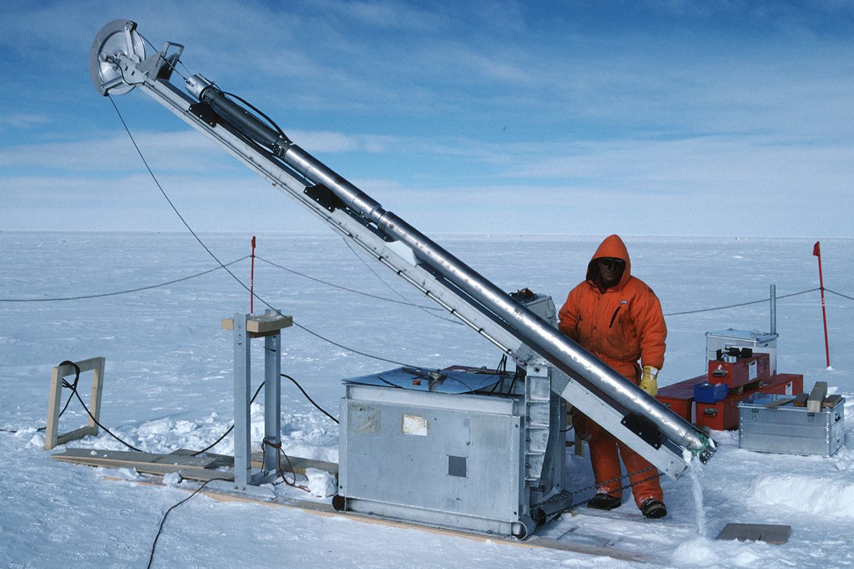


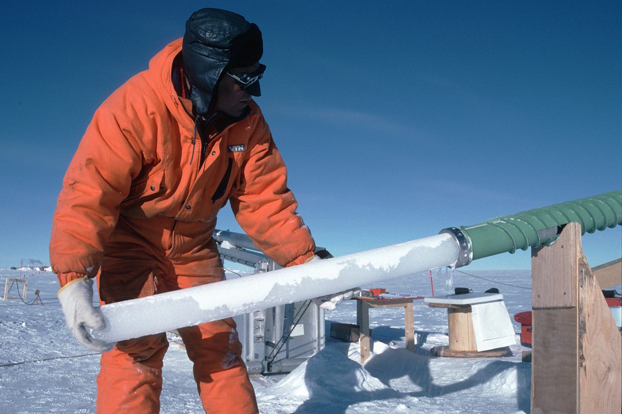


 Here, c is heat capacity, T is temperature, t is time, F Sw is the mean incoming shortwave radiation at the ground, α is albedo, ɛ is the effective emissivity, describing the partial opaqueness of the atmosphere to outgoing longwave radiation, and σ is the Stefan–Boltzmann constant. In a warmer climate, the albedo of the Earth is likely to decrease because of the smaller extent of snow and ice. Following ref. 6, we approximate this temperature dependence of the albedo as linear and set
 Subtracting Eq. 1 from Eq. 2 leads to
  If the bracketed expression on the right-hand side is larger than zero, any small temperature change ΔT would grow rapidly, and an unstable feedback would be established. Introducing σ = 5.67 · 10−8 W m−2 K−4 and mean Arctic values of F Sw = 173 W/m2, T = 255 K (see ref. 7), the bracketed expression in Eq. 3 reduces to the stability criterion
  for an isolated ice cover in the Arctic.


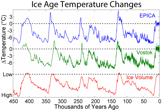

Tidak ada komentar:
Posting Komentar