Control & Optimization Electronics


The development of electronics materials and media to e - ASASS (Automatic Start And Stop System) and energy efficiency as well as its storage in electronic media to go out and visit places outside the earth orbit .
Integrated Circuits & Power Electronics
the application-driven design of electronic circuits and systems, spanning a wide spectrum from low frequencies to mm-wave and THz. The research incorporates a variety of technologies, ranging from emerging nano and MEMS devices, nano-CMOS and BiCMOS processes, as well as discrete electronics for power conversion. The specific research thrusts include:
- Mixed-signal integrated circuit design (data converters, sensor interfaces, imaging and selected areas of bio-instrumentation);
- RF and mm-wave integrated circuit design (wide band communication systems, microwave and millimeter-wave imaging, phased arrays, integrated antennas);
- Power electronics (switch-mode power converters, resonant converters; switched mode RF power amplifiers passive component design, converters using SiC and GaN at 10s of MHz, high voltage supplies, wireless power transfer systems, pulsed power applications, high voltage supplies, wireless power transfer systems, pulsed power applications);
- Nano systems (digital and analog circuits and systems) enabled by emerging nanotechnologies, including aspects of design methodology, validation and test, approximate computing, and robust circuits and systems;
- Silicon technology modeling both for digital and analog circuits, including optoelectronics / RF applications, bio-sensors and computer-aided bio-sensor design, wireless implantable sensors.
Energy-Efficient Hardware Systems
The exponential growth in performance and storage capacity has been the key enabler for information technology for decades. However, the end of voltage scaling in semiconductor chips has made all computer systems, from mobile phones to massive data centers, energy limited. Moreover, new nano systems enabled by emerging nanotechnologies provide unique opportunities for revolutionizing energy-efficient architectures through new transistor and memory technologies and their massive and fine-grained integration. These shifts motivate new system architectures and vertical co-design of hardware, system software, and applications. We look at new ways to design, architect, and manage highly energy-efficient systems for emerging applications ranging from the internet-of-things to big data analytics. Examples include:
- Hardware design for specialized accelerators and programming models for heterogeneous computing;
- Scalable architectures with thousands of computing elements and massive memory capacity;
- Hardware architectures and systems software for cloud computing;
- Architectures for nano systems enabled by emerging technologies;
- Robust and trustworthy architectures.
Biomedical Devices, Sensors & Systems
Biological properties can be measured and altered using electronics, magnetics, photonics, sensors, circuits, and algorithms. Applications range from basic biological science to clinical medicine, and enable new discoveries, diagnoses, and treatments by creating novel circuits, devices, systems, and analyses. Examples include:
- Measuring molecular concentrations
- Measuring and altering activity of electrically-excitable cells such as neurons
- Building implantable bio-sensors, bio-stimulators, and closed-loop delivery systems
- Brain-machine interfaces
- On-chip imaging and sensing
- Photonic systems for in vivo imaging
- DNA synthesis and sequencing
- Nucleic acid synthesis, sequencing and analysis
- THz and differential phase contrast x-ray imaging
- Wireless sensing and powering
- Constructing low-cost devices for point-of-care medical applications
- Designing new algorithms and systems for early cancer screening and detection
Signal Processing & Multimedia
Extracting or recovering useful information while reducing unwanted noise can be achieved using sophisticated mathematical methods and computation to process signals (audio, video, electromagnetic, biomedical, remote sensing, multimedia and others). Applications include multimedia compression, communications, networked media systems, augmented reality, and remote sensing. In addition to using theoretical analyses and systematic experiments to study the underlying principles, we often build real‐time test beds and prototypes to validate and demonstrate our ideas. Examples include:
- Image and video coding,
- Media streaming,
- Augmented and virtual reality,
- Compact descriptors for visual search,
- Personalized and immersive media,
- Computational imaging and display.
Communications Systems
Communications challenges exist over wireline, optical, and wireless links, and our research spans the study of fundamental limits, physical modeling, coding, networking and overall system design. The focus is on improving utility to users, power efficiency, and reliability. Examples include:
- Cellular and adhoc networks,
- Full duplex radio,
- Wireless communications,
- Optical communications,
- Data center networking,
- Sensor networks.
Machine Learning
Machine learning theory and applications. Examples include:
- Supervised learning,
- Unsupervised learning,
- Reinforcement learning,
- Applications
Data Science
All aspects of data and information are part of this research, including how to collect, store, organize, search, and analyze information. Recently there has been energized interest in information management because huge volumes of data are now available from sources such as web query logs, Twitter posts, blogs, satellites, sensors, and medical devices. The interest is not solely due to the volume, but because there has been a paradigm shift in the way data is used. In the past, data was used to verify hypotheses; today, mining data for patterns and trends leads to new hypotheses. The more data available, the finer and more sophisticated these hypotheses can be. Examples include:
- Managing uncertain/approximate data and models;
- Tracking data lineage;
- Causality;
- Automated data cleansing (e.g., entity resolution, graph alignment, etc.);
- Scalable self-tuning optimization, machine learning, and data mining systems;
- Algorithms for analysis of large, dynamic networks;
- Next generation distributed large-scale computing and simulation environments;
- Domain-specific languages and optimization systems for big data analytics;
- Scalable analysis tools for automatic bug detection;
- Data visualization.
OPTIMIZATION COUNT ROLLING AND EFFICIENCY
Optimal design and engineering systems operation methodology is applied to things like integrated circuits, vehicles and autopilots, energy systems (storage, generation, distribution, and smart devices), and financial trading. Optimization is also widely used in signal processing, statistics, and machine learning as a method for fitting parametric models to observed data. Examples include:
- Languages and solvers for convex optimization,
- Distributed convex optimization,
- Robotics,
- Smart grid algorithms,
- Learning via low rank models,
- Approximate dynamic programming,
- Methods for sparse signal recovery,
- Dynamic game theory,
- Control theory,
- Decentralized control.
Information Theory & Applications
Information theory, including the efficient storage, compression, and transmission of information, applies to a wide range of domains, such as communications, genomics, neuroscience, and statistics. Examples include:
- Compression,
- Coding,
- Network information theory,
- Computational genomics,
- Information theory of high dimensional statistics,
- Machine learning,
- Information flow in neural systems.
Biomedical Imaging
Basic science questions, as well as clinical applications and translation in collaboration with investigators from the Stanford School of Medicine, are applied to a broad range of imaging technologies – from devices to systems to algorithms – for biomedical applications ranging from microscopy to whole-body diagnostic imaging and image-guided interventions. Examples include:
- Optics,
- Ultrasound,
- Multiphysics approaches including photoacoustic and thermoacoustic imaging systems,
- Optical coherence tomography (OCT)
- Computed tomography (CT),
- Positron emission tomography (PET),
- Magnetic resonance imaging (MRI),
- Focused ultrasound surgery (FUS),
- Differential 3-D Phase Contrast X-ray Imaging,
- Image processing and understanding,
- Image visualization and guided interventions (including mixed reality),
- Electrophysiology and Imaging,
- Computational microscopy.
Energy Harvesting & Conversion
electronics and photonics play a central role for energy harvesting and conversion. For example, the harvesting of solar energy requires significant advance in both electronics and photonics. In addition, the majority of electronics today are fundamentally limited by the energy they consume. Conversely, the availability of more varied energy sources would enable functionality and ubiquity of electronics not yet possible today. Even when power is readily available, some electronics must obey very strict thermal requirements, such as those that come in contact with the human body. Examples include:
- Thermoelectric nanomaterials for thermal energy harvesting;
- Fundamental research into the nanoscale physics of electron-phonon energy interaction;
- Heat-sensitive electronics and their interaction with strict temperature environments such as car engines, the human body, or extraterrestrial applications;
- Energy harvesting from vibrations (piezoelectrics), thermo-acoustic energy conversion, and chemical reactions;
- Renewable energy research including photovoltaics, thermophotovoltaics and radiative cooling.
Electronic Devices
New and innovative materials, structures, process, and design technologies are explored for nanoelectronics, energy, environment, and bio-medical applications. Examples include:
- Silicon, germanium, and III-V compound semiconductor devices, metal gate/high-k MOS, and interconnects for nanoelectronics;
- Device applications of new materials such as carbon (carbon nanotube, graphene), two-dimensional (2D) layered materials (e.g. MoS2, BN) and semiconductor nanowires;
- Memory devices such as Flash, phase change memory, metal oxide resistive switching memory;
- New fabrication technologies for scaling logic and memory devices into the nanometer regime, 3D-integrated circuits with multiple layers of heterogeneous devices, metal, and optical interconnections;
- Compact modeling, technology computer aided design, and ab initio modeling of electronic materials and devices;
- Magnetic nanotechnologies and information storage.
Mobile Networking
As personal computing and data move to the cloud, mobile wireless networks form the substrate over which users access these services. Our research aims to design and build the next generation of wireless networks, taking a cross-disciplinary approach that tackles broad cross-cutting problems such as interference, mobility, and network complexity using tools from RF circuits, signal processing, communications and information theory, and distributed software systems. Examples include:
- New network designs that embrace and exploit interference instead of avoiding or ignoring it in order to create high capacity wireless networks;
- Programmable wireless infrastructure that expose interfaces for fine-grained control of the radio spectrum;
- Software systems that manage such large dense networks automatically and continuously to maximize spectral efficiency, facilitate seamless hand off between networks, and enable new services to be deployed easily in wireless networks.
Electronic circuit
An electronic circuit is composed of individual electronic components, such as resistors, transistors, capacitors, inductors and diodes, connected by conductive wires or traces through which electric current can flow. To be referred to as electronic, rather than electrical, generally at least one active component must be present. The combination of components and wires allows various simple and complex operations to be performed: signals can be amplified, computations can be performed, and data can be moved from one place to another.
Circuits can be constructed of discrete components connected by individual pieces of wire, but today it is much more common to create interconnections by photolithographic techniques on a laminated substrate (a printed circuit board or PCB) and solder the components to these interconnections to create a finished circuit. In an integrated circuit or IC, the components and interconnections are formed on the same substrate, typically a semiconductor such as silicon or (less commonly) gallium arsenide.[2]
An electronic circuit can usually be categorized as an analog circuit, a digital circuit, or a mixed-signal circuit (a combination of analog circuits and digital circuits).
Breadboards, perfboards, and stripboards are common for testing new designs. They allow the designer to make quick changes to the circuit during development.

Analog circuits

Analog electronic circuits are those in which current or voltage may vary continuously with time to correspond to the information being represented. Analog circuitry is constructed from two fundamental building blocks: series and parallel circuits.
In a series circuit, the same current passes through a series of components. A string of Christmas lights is a good example of a series circuit: if one goes out, they all do.
In a parallel circuit, all the components are connected to the same voltage, and the current divides between the various components according to their resistance.

The basic components of analog circuits are wires, resistors, capacitors, inductors, diodes, and transistors. (In 2012 it was demonstrated that memristors can be added to the list of available components.) Analog circuits are very commonly represented in schematic diagrams, in which wires are shown as lines, and each component has a unique symbol. Analog circuit analysis employs Kirchhoff's circuit laws: all the currents at a node (a place where wires meet), and the voltage around a closed loop of wires is 0. Wires are usually treated as ideal zero-voltage interconnections; any resistance or reactance is captured by explicitly adding a parasitic element, such as a discrete resistor or inductor. Active components such as transistors are often treated as controlled current or voltage sources: for example, a field-effect transistor can be modeled as a current source from the source to the drain, with the current controlled by the gate-source voltage.
An alternative model is to take independent power sources and induction as basic electronic units; this allows modeling frequency dependent negative resistors, gyrators, negative impedance converters, and dependent sources as secondary electronic components.
When the circuit size is comparable to a wavelength of the relevant signal frequency, a more sophisticated approach must be used, the distributed element model. Wires are treated as transmission lines, with nominally constant characteristic impedance, and the impedances at the start and end determine transmitted and reflected waves on the line. Circuits designed according to this approach are distributed element circuits. Such considerations typically become important for circuit boards at frequencies above a GHz; integrated circuits are smaller and can be treated as lumped elements for frequencies less than 10GHz or so.
Digital circuits
In digital electronic circuits, electric signals take on discrete values, to represent logical and numeric values.[3] These values represent the information that is being processed. In the vast majority of cases, binary encoding is used: one voltage (typically the more positive value) represents a binary '1' and another voltage (usually a value near the ground potential, 0 V) represents a binary '0'. Digital circuits make extensive use of transistors, interconnected to create logic gates that provide the functions of Boolean logic: AND, NAND, OR, NOR, XOR and all possible combinations thereof. Transistors interconnected so as to provide positive feedback are used as latches and flip flops, circuits that have two or more metastable states, and remain in one of these states until changed by an external input. Digital circuits therefore can provide both logic and memory, enabling them to perform arbitrary computational functions. (Memory based on flip-flops is known as static random-access memory (SRAM). Memory based on the storage of charge in a capacitor, dynamic random-access memory (DRAM) is also widely used.)
The design process for digital circuits is fundamentally different from the process for analog circuits. Each logic gate regenerates the binary signal, so the designer need not account for distortion, gain control, offset voltages, and other concerns faced in an analog design. As a consequence, extremely complex digital circuits, with billions of logic elements integrated on a single silicon chip, can be fabricated at low cost. Such digital integrated circuits are ubiquitous in modern electronic devices, such as calculators, mobile phone handsets, and computers. As digital circuits become more complex, issues of time delay, logic races, power dissipation, non-ideal switching, on-chip and inter-chip loading, and leakage currents, become limitations to the density, speed and performance.
Digital circuitry is used to create general purpose computing chips, such as microprocessors, and custom-designed logic circuits, known as application-specific integrated circuit (ASICs). Field-programmable gate arrays (FPGAs), chips with logic circuitry whose configuration can be modified after fabrication, are also widely used in prototyping and development.
Mixed-signal circuits
Mixed-signal or hybrid circuits contain elements of both analog and digital circuits. Examples include comparators, timers, phase-locked loops, analog-to-digital converters, and digital-to-analog converters. Most modern radio and communications circuitry uses mixed signal circuits. For example, in a receiver, analog circuitry is used to amplify and frequency-convert signals so that they reach a suitable state to be converted into digital values, after which further signal processing can be performed in the digital domain.
Electronic circuit design
Electronic circuit design comprises the analysis and synthesis of electronic circuits.
Methods
To design any electrical circuit, either analog or digital, electrical engineers need to be able to predict the voltages and currents at all places within the circuit. Linear circuits, that is, circuits wherein the outputs are linearly dependent on the inputs, can be analyzed by hand using complex analysis. Simple nonlinear circuits can also be analyzed in this way. Specialized software has been created to analyze circuits that are either too complicated or too nonlinear to analyze by hand.
Circuit simulation software allows engineers to design circuits more efficiently, reducing the time cost and risk of error involved in building circuit prototypes. Some of these make use of hardware description languages such as VHDL or Verilog.
Network simulation software
Linearization around operating point
When faced with a new circuit, the software first tries to find a steady state solution wherein all the nodes conform to Kirchhoff's Current Law and the voltages across and through each element of the circuit conform to the voltage/current equations governing that element.
Once the steady state solution is found, the software can analyze the response to perturbations using piecewise approximation, harmonic balance or other methods.
Piece-wise linear approximation
Software such as the PLECS interface to Simulink uses piecewise linear approximation of the equations governing the elements of a circuit. The circuit is treated as a completely linear network of ideal diodes. Every time a diode switches from on to off or vice versa, the configuration of the linear network changes. Adding more detail to the approximation of equations increases the accuracy of the simulation, but also increases its running time.
Synthesis
Simple circuits may be designed by connecting a number of elements or functional blocks such as integrated circuits.
An efficient integrated interface electronics for electromagnetic energy harvesting from low voltage sources
A fully-integrated self-powered interface circuit for efficient rectification of the signals generated by vibration based low-voltage electromagnetic (EM) energy harvesters. The circuit utilizes an improved AC/DC doubler structure with active diodes to minimize the forward bias voltage drop for enhancing the rectifier efficiency. The comparators in the active diodes are powered internally by another passive AC/DC doubler with diode connected transistors. The performance is maximized through custom-designed comparators for each of the positive and negative terminals of the dual rail output. Measurement results show that the system is capable of driving 40 μA load at 0.61 V, with 67% power conversion efficiency, when operated together with an inhouse EM harvester subjected to vibrations at 10 Hz, 2.5 mm peak-to-peak displacement with 0.5 g acceleration. The circuit is able to rectify AC inputs with peak amplitude as low as 100 mV.


Innovative energy electronic devices and sensors are being created for Social Innovation by controlling charged particles for nanometer-order micro-fabrication, and electronic integrated circuits design technology.
Research Themes of Electronics
Energy electronic devices

Next-generation power modules for societal infrastructure products such as rolling stock, wind turbines and vehicles are being developed.
Sensing

High reliability sensor devices and applications are being developed to contribute to a safer and more comfortable society.
Energy electronic devices
Research Themes of Electronics
Next-generation power modules for societal infrastructure products such as rolling stock, wind turbines and vehicles are being developed.
By improving power conversion efficiency, the modules contribute to greater energy saving of these innovative products. Further by reducing their size, the weight of the vehicles are reduced and further energy saving is achieved.
By improving power conversion efficiency, the modules contribute to greater energy saving of these innovative products. Further by reducing their size, the weight of the vehicles are reduced and further energy saving is achieved.

Sensing
Research Themes of Electronics
High reliability sensor devices and applications are being developed to contribute to a safer and more comfortable society.
Using MEMS* structural design which has a high tolerance for harsh environments, sensors such as those for automotive vehicles which operate under harsh vibration and temperature conditions are being created.
Using MEMS* structural design which has a high tolerance for harsh environments, sensors such as those for automotive vehicles which operate under harsh vibration and temperature conditions are being created.
* MEMS: Micro Electro Mechanical Systems

XO____ XO XXX Hidden Portals in Earth's Magnetic Field
A favorite theme of science fiction is "the portal"--an extraordinary opening in space or time that connects travelers to distant realms. A good portal is a shortcut, a guide, a door into the unknown. If only they actually existed....
It turns out that they do, sort of, and a NASA-funded researcher at the University of Iowa has figured out how to find them.
"We call them X-points or electron diffusion regions," explains plasma physicist Jack Scudder of the University of Iowa. "They're places where the magnetic field of Earth connects to the magnetic field of the Sun, creating an uninterrupted path leading from our own planet to the sun's atmosphere 93 million miles away."
Observations by NASA's THEMIS spacecraft and Europe's Cluster probes suggest that these magnetic portals open and close dozens of times each day. They're typically located a few tens of thousands of kilometers from Earth where the geomagnetic field meets the onrushing solar wind. Most portals are small and short-lived; others are yawning, vast, and sustained. Tons of energetic particles can flow through the openings, heating Earth's upper atmosphere, sparking geomagnetic storms, and igniting bright polar auroras.
NASA is planning a mission called "MMS," short for Magnetospheric Multiscale Mission, due to launch in 2014, to study the phenomenon. Bristling with energetic particle detectors and magnetic sensors, the four spacecraft of MMS will spread out in Earth's magnetosphere and surround the portals to observe how they work.
Just one problem: Finding them. Magnetic portals are invisible, unstable, and elusive. They open and close without warning "and there are no signposts to guide us in," notes Scudder.
Actually, there are signposts, and Scudder has found them.
Portals form via the process of magnetic reconnection. Mingling lines of magnetic force from the sun and Earth criss-cross and join to create the openings. "X-points" are where the criss-cross takes place. The sudden joining of magnetic fields can propel jets of charged particles from the X-point, creating an "electron diffusion region."
To learn how to pinpoint these events, Scudder looked at data from a space probe that orbited Earth more than 10 years ago.
"In the late 1990s, NASA's Polar spacecraft spent years in Earth's magnetosphere," explains Scudder, "and it encountered many X-points during its mission."

Because Polar carried sensors similar to those of MMS, Scudder decided to see how an X-point looked to Polar. "Using Polar data, we have found five simple combinations of magnetic field and energetic particle measurements that tell us when we've come across an X-point or an electron diffusion region. A single spacecraft, properly instrumented, can make these measurements."
This means that single member of the MMS constellation using the diagnostics can find a portal and alert other members of the constellation. Mission planners long thought that MMS might have to spend a year or so learning to find portals before it could study them. Scudder's work short cuts the process, allowing MMS to get to work without delay.
It's a shortcut worthy of the best portals of fiction, only this time the portals are real. And with the new "signposts" we know how to find them.
A NASA-sponsored researcher at the University of Iowa has developed a way for spacecraft to hunt down hidden magnetic portals in the vicinity of Earth. These gateways link the magnetic field of our planet to that of the sun, setting the stage for stormy space weather.
XO____XO XXX 10001 + 10 Discoveries of exoplanets
An exoplanet (extrasolar planet) is a planet located outside the Solar System. The first evidence of an exoplanet was noted as early as 1917, but was not recognized as such. However, the first scientific detection of an exoplanet began in 1988. Shortly afterwards, the first confirmed detection came in 1992, with the discovery of several terrestrial-mass planets orbiting the pulsar PSR B1257+12. The first confirmation of an exoplanet orbiting a main-sequence star was made in 1995, when a giant planet was found in a four-day orbit around the nearby star 51 Pegasi. Some exoplanets have been imaged directly by telescopes, but the vast majority have been detected through indirect methods, such as the transit method and the radial-velocity method. As of 1 July 2018, there are 3,797 confirmed planets in 2,841 systems, with 632 systems having more than one planet.This is a list of the most notable discoveries.


1988–1994
- Gamma Cephei Ab: The radial velocity variations of the star Gamma Cephei were announced in 1989, consistent with a planet in a 2.5-year orbit.[4] However, misclassification of the star as a giant combined with an underestimation of the orbit of the Gamma Cephei binary, which implied the planet's orbit would be unstable, led some astronomers to suspect the variations were merely due to stellar rotation. The existence of the planet was finally confirmed in 2002.[5][6]
- HD 114762 b: This object has a minimum mass 11 times the mass of Jupiter and has an 89-day orbit. At the time of its discovery it was regarded as a probable brown dwarf,[7] although subsequently it has been included in catalogues of extrasolar planets.[8][9]
- PSR B1257+12: The first confirmed discovery of extrasolar planets was made in 1992 when a system of terrestrial-mass planets was announced to be present around the millisecond pulsar PSR B1257+12.[2]
1995–1998
- 51 Pegasi b: In 1995 this became the first exoplanet orbiting a main-sequence star to have its existence confirmed. It is a hot Jupiter with a 4.2-day orbit.[10]
- 47 Ursae Majoris b: In 1996 this Jupiter-like planet was the first long-period planet discovered, orbiting at 2.11 AU from the star with the eccentricity of 0.049. There is a second companion that orbits at 3.39 AU with the eccentricity of 0.220 ± 0.028 and a period of 2190 ± 460 days.
- Gliese 876 b: In 1998, the first planet was found that orbits around a red dwarf star (Gliese 876). It is closer to its star than Mercury is to the Sun. More planets have subsequently been discovered even closer to the star.[11]
1999
- Upsilon Andromedae: The first multiple-planetary system to be discovered around a main sequence star. It contains three planets, all of which are Jupiter-like. Planets b, c, d were announced in 1996, 1999, and 1999 respectively. Their masses are 0.687, 1.97, and 3.93 MJ; they orbit at 0.0595, 0.830, and 2.54 AU respectively.[12] In 2007 their inclinations were determined as non-coplanar.
- HD 209458 b: After being originally discovered with the radial-velocity method, this became the first exoplanet to be seen transiting its parent star. The transit detection conclusively confirmed the existence of the planets suspected to be responsible for the radial velocity measurements.[13][14]
2001
- HD 209458 b: Astronomers using the Hubble Space Telescope announced that they had detected the atmosphere of HD 209458 b. They found the spectroscopic signature of sodium in the atmosphere, but at a smaller intensity than expected, suggesting that high clouds obscure the lower atmospheric layers.[15] In 2008 the albedo of its cloud layer was measured, and its structure modeled as stratospheric.
- Iota Draconis b: The first planet discovered around the giant star Iota Draconis, an orange giant. This provides evidence for the survival and behavior of planetary systems around giant stars. Giant stars have pulsations that can mimic the presence of planets. The planet is very massive and has a very eccentric orbit. It orbits on average 27.5% further from its star than Earth does from the Sun.[16] In 2008 the system's origin would be traced to the Hyades cluster, alongside Epsilon Tauri.
2003
- PSR B1620-26 b: On July 10, using information obtained from the Hubble Space Telescope, a team of scientists led by Steinn Sigurðsson confirmed the oldest extrasolar planet yet. The planet is located in the globular star cluster M4, about 5,600 light years from Earth in the constellation Scorpius. This is one of only three planets known to orbit around a stellar binary; one of the stars in the binary is a pulsar and the other is a white dwarf. The planet has a mass twice that of Jupiter, and is estimated to be 12.7 billion years old.[17]
2004
- Mu Arae c: In August, a planet orbiting Mu Arae with a mass of approximately 14 times that of the Earth was discovered with the European Southern Observatory's HARPS spectrograph. Depending on its composition, it is the first published "hot Neptune" or "super-Earth".[18]

- 2M1207 b: The first planet found around a brown dwarf. The planet is also the first to be directly imaged (in infrared). According to an early estimate, it has a mass 5 times that of Jupiter; other estimates give slightly lower masses. It was originally estimated to orbit at 55 AU from the brown dwarf. The brown dwarf is only 25 times as massive as Jupiter. The temperature of the gas giant planet is very high (1250 K), mostly due to gravitational contraction.[19] In late 2005, the parameters were revised to orbital radius 41 AU and mass of 3.3 Jupiters, because it was found that the system is closer to Earth than was originally believed. In 2006, a dust disk was found around 2M1207, providing evidence for active planet formation.[20]
2005
- TrES-1 and HD 209458b: On March 22, two groups announced the first direct detection of light emitted by exoplanets, achieved with the Spitzer Space Telescope. These studies permitted the direct study of the temperature and structure of the planetary atmospheres.[21][22]
- Gliese 876 d: On June 13, a third planet orbiting the red dwarf star Gliese 876 was announced. With a mass estimated at 7.5 times that of Earth, it may be rocky in composition. The planet orbits at 0.021 AU with a period of 1.94 days.[23]
- HD 149026 b: This planet was announced on July 1. Its unusually high density indicated that it was a giant planet with a large core, the largest one yet known. The mass of the core was estimated at 70 Earth masses (as of 2008, 80-110), accounting for at least two-thirds of the planet's total mass.[24]
2006
- OGLE-2005-BLG-390Lb: This planet, announced on January 25, was detected using the gravitational microlensing method. It orbits a red dwarf star around 21,500 light years from Earth, toward the center of the Milky Way galaxy. As of April 2010, it remains the most distant known exoplanet. Its mass is estimated to be 5.5 times that of Earth. Prior to this discovery, the few known exoplanets with comparably low masses had only been discovered in orbits very close to their parent stars, but this planet is estimated to have a relatively wide separation of 2.6 AU from its parent star. Due to that wide separation and due to the inherent dimness of the star, the planet is probably the coldest exoplanet known.[25][26]
- HD 69830: Has a planetary system with three Neptune-mass planets. It is the first triple planetary system without any Jupiter-like planets discovered around a Sun-like star. All three planets were announced on May 18 by Lovis. All three orbit within 1 AU. The planets b, c and d have masses of 10, 12 and 18 times that of Earth, respectively. The outermost planet, d, appears to be in the habitable zone, shepherding a thick asteroid belt.[27]
2007
- HD 209458 b and HD 189733 b: These became the first extrasolar planets to have their atmospheric spectra directly observed. The announcement was made on February 21, by two groups of researchers who had worked independently.[28] One group, led by Jeremy Richardson of NASA's Goddard Space Flight Center, observed the atmosphere of HD 209458 b over a wavelength range from 7.5 to 13.2 micrometres. The results were surprising in several ways. The 10-micrometre spectral peak of water vapor was absent. An unpredicted peak was observed at 9.65 micrometres, which the investigators attributed to clouds of silicate dust. Another peak, at 7.78 micrometres, remained unexplained.[29] The other group, led by Carl Grillmair of NASA's Spitzer Science Center, observed HD 189733 b. They also failed to detect the spectroscopic signature of water vapor.[30] Later in the year, yet another group of researchers using a somewhat different technique succeeded in detecting water vapor in the planet's atmosphere, the first time such a detection had been made.[31][32]
- Gliese 581 c: A team of astronomers led by Stephane Udry used the HARPS instrument on the European Southern Observatory's 3.6-meter telescope to discover this exoplanet by means of the radial velocity method.[33] The team calculated that the planet could support liquid water and possibly life.[34] However, subsequent habitability studies indicate that the planet likely suffers from a runaway greenhouse effect similar to Venus, rendering the presence of liquid water impossible.[35][36] These studies suggest that the third planet in the system, Gliese 581 d, is more likely to be habitable. Seth Shostak, a senior astronomer with the SETI institute, stated that two unsuccessful searches had already been made for radio signals from extraterrestrial intelligence in the Gliese 581 system.[34]
- Gliese 436 b: This planet was one of the first Neptune-mass planets discovered, in August 2004. In May 2007, a transit was found, revealed as the smallest and least massive transiting planet yet at 22 times that of Earth. Its density is consistent with a large core of an exotic form of solid water called "hot ice", which would exist, despite the planet's high temperatures, because the planet's gravity causes water to be extremely dense.[37]
- TrES-4: The largest-diameter and lowest-density exoplanet to date, TrES-4 is 1.7 times Jupiter's diameter but only 0.84 times its mass, giving it a density of just 0.2 grams per cubic centimeter—about the same as balsa wood. It orbits its primary closely and is therefore quite hot, but stellar heating alone does not appear to explain its large size.[38]
2008
- OGLE-2006-BLG-109Lb and OGLE-2006-BLG-109Lc: On February 14, the discovery of a planetary system was announced that is the most similar one known to the Jupiter-Saturn pair within the Solar System in terms of mass ratio and orbital parameters. The presence of planets with such parameters has implications for possible life in a solar system as Jupiter and Saturn have a stabilizing effect to the habitable zone by sweeping away large asteroids from the habitable zone.[39]
- HD 189733 b: On March 20, follow-up studies to the first spectral analyses of an extrasolar planet were published in the scientific journal Nature, announcing evidence of an organic molecule found on an extrasolar planet for the first time. The analysis showed not only water vapor, but also methane existing in the atmosphere of the giant gas planet. Although conditions on there are too harsh to harbor life, it still is the first time a key molecule for organic life was found on an extrasolar planet.[40]
- HD 40307: On June 16, Michel Mayor announced a planetary system with three super-Earths orbiting this K-type star. The planets have masses ranging from 4 to 9 Earth masses and periods ranging from 4 to 20 days. It was suggested this might be the first multi-planet system without any known gas giants. However, a subsequent study of the system's orbital stability found that tidal interactions have had little effect on evolution of the planets' orbits. That, in turn, suggests that the planets experience relatively low tidal dissipation and hence are of primarily gaseous composition.[41] All three were discovered by the HARPS spectrograph in La Silla, Chile.[42]
- 1RXS J160929.1−210524: In September, an object was imaged in the infrared at a separation of 330AU from this star. Later, in June 2010, the object was confirmed to be a companion planet to the star rather than a background object aligned by chance.[43]
- Fomalhaut b: On November 13, NASA and the Lawrence Livermore National Laboratory announced the discovery of an extrasolar planet orbiting just inside the debris ring of the A class star Fomalhaut (Alpha Piscis Austrini). This was the first extrasolar planet to be directly imaged by an optical telescope.[44] Its mass is estimated to be three times that of Jupiter.[45][46] Based on the planet's unexpected brightness at visible wavelengths, the discovery team suspects it is surrounded by its own large disk or ring that may be a satellite system in the process of formation.
- HR 8799: Also on November 13, the discovery of three planets orbiting HR 8799 was announced. This was the first direct image of multiple planets. Christian Marois of the National Research Council of Canada's Herzberg Institute of Astrophysics and his team used the Keck and Gemini telescopes in Hawaii. The Gemini images allowed the international team to make the initial discovery of two of the planets with data obtained on October 17, 2007. Then, in July through September 2008 the team confirmed this discovery and found a third planet orbiting even closer to the star with images obtained at the Keck II telescope. A review of older data taken in 2004 with the Keck II telescope revealed that the outer 2 planets were visible on these images. Their masses and separations are approximately 7 MJ at 24 AU, 7 MJ at 38 AU, and 5 MJ at 68 AU.[46][47]
2009
- COROT-7b: On February 3, the European Space Agency announced the discovery of a planet orbiting the star COROT-7. Although the planet orbits its star at a distance less than 0.02 AU, its diameter is estimated to be around 1.7 times that of Earth, making it the smallest super-Earth yet measured. Due to its extreme closeness to its parent star, it is believed to have a molten surface at a temperature of 1000–1500 °C.[48] It was discovered by the French COROT satellite.
- Gliese 581 e: On April 21, the European Southern Observatory announced the discovery of a fourth planet orbiting the star Gliese 581. The planet orbits its parent star at a distance of less than 0.03 AU and has a minimum mass estimated at 1.9 times that of Earth. As of January 2010, this is the lightest known extrasolar planet to orbit a main-sequence star.[10]
- 30 planets: On October 19, it was announced that 30 new planets were discovered, all were detected by radial velocity method. It is the most planets ever announced in a single day during the exoplanet era. October 2009 now holds the most planets discovered in a month, breaking the record set in June 2002 and August 2009, during which 17 planets were discovered.
- 61 Virginis and HD 1461: On December 14, three planets (one is super-Earth and two are Neptune-mass planets) were discovered. Also a super-Earth planet and two unconfirmed planets around HD 1461 were discovered. These discoveries indicated that low-mass planets that orbit around nearby stars are very common. 61 Virginis is the first star like the Sun to host the super-Earth planets.[49]
- GJ 1214 b: On December 16, a super-Earth planet was discovered by transit. The determination of density from mass and radius suggest that this planet may be an ocean planet composed of 75% water and 25% rock. Some of the water on this planet should be in the exotic form of ice VII. This is the first planet discovered by MEarth Project, which is used to look for transits of super-Earth planets crossing the face of M-type stars.[50]
2010
- 47 Ursae Majoris d: On March 6, a gas giant like Jupiter with the longest known orbital period for any exoplanet was detected via radial velocity. It orbits its parent star at a distance similar to Saturn in the Solar System with its orbital period lasting about 38 Earth years.
- COROT-9b: On March 17, the first known temperate transiting planet was announced. Discovered by the COROT satellite, it has an orbital period of 95 days and a periastron distance of 0.36 AU, by far the largest of any exoplanet whose transit has been observed. The temperature of the planet is estimated at between 250 K and 430 K (between -20 °C and 160 °C).[51]
- Beta Pictoris b: On June 10, for the first time astronomers have been able to directly follow the motion of an exoplanet as it moves to the other side of its host star. The planet has the smallest orbit so far of all directly imaged exoplanets, lying as close to its host star as Saturn is to the Sun.[52]
- HD 209458 b: On June 23, astronomers announced they have measured a superstorm for the first time in the atmosphere of HD 209458 b. The very high-precision observations done by ESO’s Very Large Telescope and its powerful CRIRES spectrograph of carbon monoxide gas show that it is streaming at enormous speed from the extremely hot day side to the cooler night side of the planet. The observations also allow another exciting “first” — measuring the orbital speed of the exoplanet itself, providing a direct determination of its mass.[53]
- HD 10180: On August 24, astronomers using ESO’s HARPS instrument announced the discovery of a planetary system with up to seven planets orbiting a Sun-like star with five confirmed Neptune-mass planets and evidence of two other planets, one of which could have the lowest mass of any planet found to date orbiting a main-sequence star, and the other of which may be a long-period Saturnian planet. Additionally, there is evidence that the distances of the planets from their star follow a regular pattern, as seen in the Solar System.
2011
- Kepler 11: On February 3, astronomers using NASA's Kepler Mission announced the discovery of 6 transiting planets orbiting the star Kepler 11. Masses were confirmed using a new method called Transit Timing Variations. The architecture of the system is unique with 6 low mass, low density planets all packed in tight orbits around their host star. The 5 inner planets all orbit inside that of Mercury in the Solar System. It is believed that these planets formed out past the snow line and migrated into their current position.[
- 55 Cancri e: On April 27, 2011, the super-earth 55 Cancri e was found to transit its host star using the MOST satellite. This planet has the shortest known orbital period of any extrasolar planet at .73 days. It is also the first time a super earth has been detected transiting a naked eye star (less than 6th magnitude in V band). The high density calculated suggests that the planet has a "rock-iron composition supplemented by a significant mass of water, gas, or other light elements".[56]
2012


- Alpha Centauri Bb: On 16 October 2012, the discovery was announced of an Earth-mass planet in orbit around Alpha Centauri B. The discovery was published online on the 17 of October, in the scientific journal Nature, and the lead author of the paper was Xavier Dumusque, a graduate student at the Centro de Astrofísica da Universidade do Porto (Centre for Astrophysics of the University of Porto). The discovery of a planet in the closest star system to Earth received widespread media attention, and was seen as an important landmark in exoplanet research.
2013
- PH2 b: On 3 January 2013, the discovery of a "Jupiter-size" extrasolar planet that could "potentially be habitable" was announced.[57][58] The exoplanet was discovered by amateur astronomers from the Planet Hunters project of amateur astronomers using data from the Kepler Mission space observatory and confirmed, with 99.9 percent confidence, by observations at the W. M. Keck Observatory in Hawaii.[58] PH2 b is the second confirmed planet discovered by PlanetHunters.org (the first being PH1).[57][58]
- Kepler-69c (formerly KOI-172.02): On 7 January 2013, the discovery of an unconfirmed (Kepler Object of Interest) candidate exoplanet was announced by astronomers affiliated with the Kepler Mission space observatory.[59][60] The candidate object, a Super-Earth, has a radius 1.54 times that of Earth. Kepler-69c orbits a sun-like star, named Kepler-69,[61] within the "habitable zone"[60] a zone where liquid water could exist on the surface of the planet. Scientists claim the exoplanet, if confirmed, could be a "prime candidate to host alien life".[60]
- On 18 April 2013, NASA announced the discovery of three new Earth-like exoplanets – Kepler-62e, Kepler-62f, and Kepler-69c (now confirmed) – in the habitable zones of their respective host stars, Kepler-62 and Kepler-69. The new exoplanets, which are considered prime candidates for possessing liquid water and thus potentially life, were identified using the Kepler space observatory.[62][63][64]
2014
- On 26 February 2014, NASA announced the discovery of 715 newly verified exoplanets around 305 stars by the Kepler Space Telescope. The exoplanets were found using a statistical technique called "verification by multiplicity". 95% of the discovered exoplanets were smaller than Neptune and four, including Kepler-296f, were less than 2 1/2 the size of Earth and were in habitable zones where surface temperatures are suitable for liquid water.[
- In November 2014, the Planet Hunters group discovered the exoplanet PH3 c. This exoplanet is 700 parsecs away from Earth, is a low density planet and is four times as massive as Earth.
- In July, 2014, NASA announced the determination of the most precise measurement so far attained for the size of an exoplanet (Kepler-93b);[70] the discovery of an exoplanet (Kepler-421b) that has the longest known year (704 days) of any transiting planet found so far;[71] and, finding very dry atmospheres on three exoplanets (HD 189733b, HD 209458b, WASP-12b) orbiting sun-like stars.[72]
2015
- On 6 January 2015, NASA announced the 1000th confirmed exoplanet discovered by the Kepler Space Telescope. Three of the newly confirmed exoplanets were found to orbit within habitable zones of their host stars: two of the three, Kepler-438b and Kepler-442b, are near-Earth-size and likely rocky; the third, Kepler-440b, is a super-Earth. Similar confirmed small exoplanets in habitable zones found earlier by Kepler include: Kepler-62e, Kepler-62f, Kepler-186f, Kepler296e and Kepler-296f.[73]
- On 23 July 2015, NASA announced the release of the Seventh Kepler Candidate Catalog, bringing the total number of confirmed exoplanets to 1030 and the number of exoplanet candidates to 4,696. This announcement also included the first report of Kepler-452b, a near-Earth-size planet orbiting the habitable zone of a G2-type star, as well as eleven other "small habitable zone candidate planets".[74]
- On 30 July 2015, NASA confirmed the discovery of the nearest rocky planet outside the Solar System, larger than Earth, 21 light-years away. HD 219134 b is the closest exoplanet to Earth to be detected transiting in front of its star. The planet has a mass 4.5 times that of Earth, a radius about 1.6 times that of Earth, with a three-day orbit around its star. Combining the size and mass gives it a density of 6 g/cm3, confirming that it is a rocky planet.[75][76][77]
- In September 2015, astronomers reported the unusual light fluctuations of KIC 8462852, an F-type main-sequence star in the constellation Cygnus, as detected by the Kepler space telescope, while searching for exoplanets. Various explanations have been presented, including those based on comets, asteroids, as well as, an alien civilization.
2016
- On August 24, 2016, the Pale Red Dot campaign announced the discovery of Proxima b. Orbiting the closest star to the solar system, Proxima Centauri, the 1.3 Earth-mass exoplanet orbits within the star's habitable zone. The planet was discovered by the HARPS and UVES instruments on telescopes at the European Southern Observatory in Chile, after signs of a planet orbiting Proxima Centauri were first found in 2013.
2017
- On 22 February 2017, several scientists working at the California Institute of Technology for NASA, using the Spitzer Space Telescope, announced the discovery of seven potentially habitable exoplanets orbiting TRAPPIST-1, a star about 40 light years away. Three of these planets are said to be located within the habitable zone of the TRAPPIST-1 solar system and have the potential to harbor liquid water on their surface and possibly sustain life. The discovery sets a new record for the greatest number of habitable-zone planets found around a single star outside our solar system.[82] TRAPPIST-1 is a red dwarf, which raises the likelihood of the exoplanets orbiting TRAPPIST-1 being tidally locked with the parent star.[83]
- Ross 128 b is a confirmed Earth-sized exoplanet, likely rocky, orbiting within the inner habitable zone of the red dwarf Ross 128. It is the second-closest potentially habitable exoplanet found, at a distance of about 11 light-years; only Proxima Centauri b is closer. The planet is only 35% more massive than Earth, receives only 38% more sunlight, and is expected to be a temperature suitable for liquid water to exist on the surface, if it has an atmosphere.[84]
2018
- Analyses show that K2-155d may fall into the habitable zone and support liquid water.[85]
- WASP-104b, a Hot Jupiter exoplanet, has been considered by researchers to be one of the darkest exoplanets ever discovered.[86]
- Helium has been detected for the first time in the atmosphere of an exoplanet by scientists observing WASP-107b.[87]
- On 7 June, scientists working at the Physical Research Laboratory (PRL) for ISRO, using the PRL Advance Radial-velocity Abu-Sky Search (Paras) spectrograph integrated with a telescope at the Mount Abu InfraRed Observatory, announced the discovery of host star EPIC 211945201 or K2-236 and exoplanet EPIC 211945201b or K2-236b. Located at a distance of 600 light years from Earth, the exoplanet has a mass 27 times heavier than that of Earth, and is 6 times its radius. K2-236b has a surface temperature of 600°C
XO___XO XXX 10001 >2 + 10 <5 the temperature on the Moon
CLIMATE: MOON
Here, the climate is cold and temperate. The rainfall in Moon is significant, with precipitation even during the driest month. The climate here is classified as Dfb by the Köppen-Geiger system. The average temperature in Moon is 9.9 °C. The rainfall here averages 967 mm.
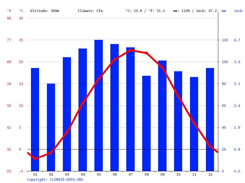
CLIMOGRAPH MOON
Precipitation is the lowest in February, with an average of 60 mm. In July, the precipitation reaches its peak, with an average of 102 mm.
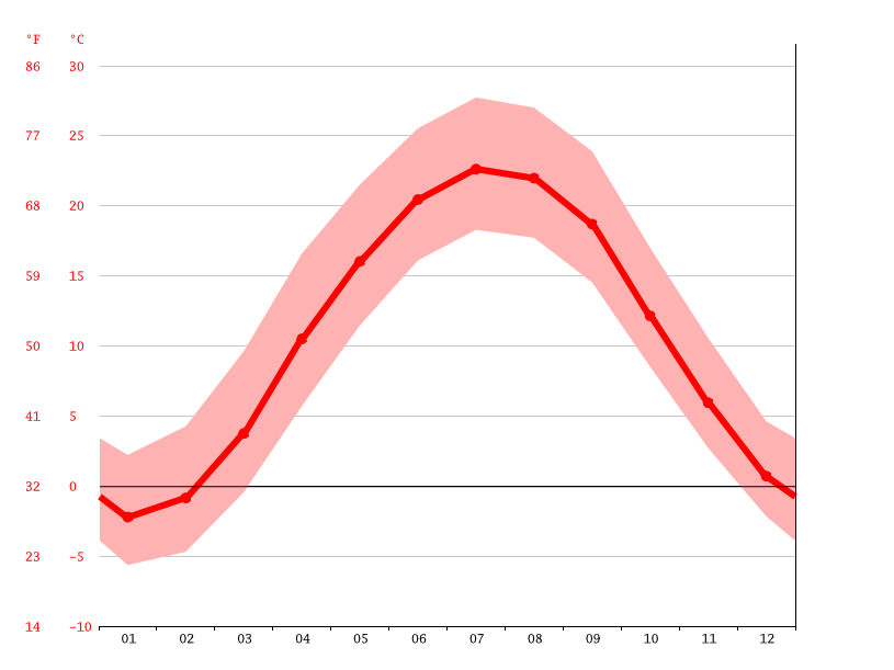
TEMPERATURE GRAPH MOON
At an average temperature of 21.9 °C, July is the hottest month of the year. At -3.2 °C on average, January is the coldest month of the year.
| January | February | March | April | May | June | July | August | September | October | November | December | |
|---|---|---|---|---|---|---|---|---|---|---|---|---|
| Avg. Temperature (°C) | -3.2 | -1.9 | 3.5 | 9.4 | 15 | 19.6 | 21.9 | 21.1 | 17.2 | 10.9 | 5.4 | -0.3 |
| Min. Temperature (°C) | -7.9 | -7.1 | -2.3 | 2.8 | 8.3 | 13 | 15.6 | 14.8 | 10.9 | 4.6 | 0.3 | -4.5 |
| Max. Temperature (°C) | 1.6 | 3.3 | 9.3 | 16 | 21.8 | 26.3 | 28.3 | 27.4 | 23.6 | 17.3 | 10.5 | 4 |
| Avg. Temperature (°F) | 26.2 | 28.6 | 38.3 | 48.9 | 59.0 | 67.3 | 71.4 | 70.0 | 63.0 | 51.6 | 41.7 | 31.5 |
| Min. Temperature (°F) | 17.8 | 19.2 | 27.9 | 37.0 | 46.9 | 55.4 | 60.1 | 58.6 | 51.6 | 40.3 | 32.5 | 23.9 |
| Max. Temperature (°F) | 34.9 | 37.9 | 48.7 | 60.8 | 71.2 | 79.3 | 82.9 | 81.3 | 74.5 | 63.1 | 50.9 | 39.2 |
| Precipitation / Rainfall (mm) | 65 | 60 | 85 | 84 | 98 | 97 | 102 | 86 | 79 | 63 | 76 | 72 |
Between the driest and wettest months, the difference in precipitation is 42 mm. The variation in annual temperature is around 25.1 °C.
Moon land is considered to have a desert climate. There is virtually no rainfall during the year in Moon land. The climate here is classified as BWh by the Köppen-Geiger system. The average annual temperature is 20.7 °C in Moon land. Precipitation here averages 21 mm.
Are you planning a trip to the Moon and you’re wondering what kinds of temperature you might experience. Well, you’re going to want to pack something to keep you warm, since the temperature of the Moon can dip down to -153°C during the night. Oh, but you’re going to want to keep some cool weather clothes too, since the temperature of the Moon in the day can rise to 107°C.
Why does the moon’s temperature vary so widely? It happens because the Moon doesn’t have an atmosphere like the Earth. Here on Earth, the atmosphere acts like a blanket, trapping heat. Sunlight passes through the atmosphere, and warms up the ground. The energy is emitted by the ground as infrared radiation, but it can’t escape through the atmosphere again easily so the planet warms up. Nights are colder than days, but it’s nothing like the Moon.
There’s another problem. The moon takes 27 days to rotate once on its axis. So any place on the surface of the Moon experiences about 13 days of sunlight, followed by 13 days of darkness. So if you were standing on the surface of the Moon in sunlight, the temperature would be hot enough to boil water. And then the Sun would go down, and the temperature would drop 250 degrees in just a matter of moments.
To deal with this dramatic range in temperature, spacesuits are heavily insulated with layers of fabric and then covered with reflective outer layers. This minimizes the temperature differences between when the astronaut is in the sunlight and when in shade. Space suits also have internal heaters and cooling systems, and liquid heat exchange pumps that remove excess heat.
There are craters around the north and south poles of the Moon which are bathed in complete shadow, and never see sunlight. This places would always be as cool as -153°C. Similarly, there are nearby mountain peaks which are bathed in continuous sunlight, and would always be hot.
We have written many articles for Universe Today about some of the special regions of the Moon. Here’s an article about building a moon base, and here’s an article about a perfect crater for a human settlement.

+++++++++++++++++++++++++++++++++++++++++++++++++++++++++++++++++++++++++++++++

++++++++++++++++++++++++++++++++++++++++++++++++++++++++++++++++++++++++++++++
Tidak ada komentar:
Posting Komentar