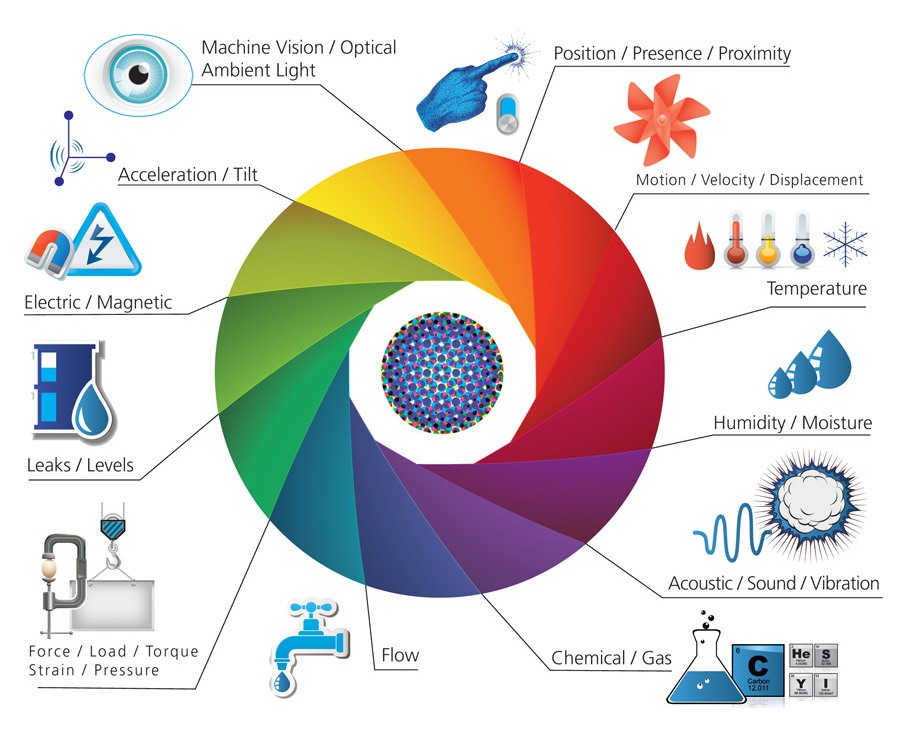


The state of clouds and the movement of clouds above the earth in communications electronics is very important in the era of now, especially for the medium of mediation the way the electronic signal in the delivery of information information both sound and image is also about geographical data data that exist on earth also in the earth orbit .
Cloud
In meteorology, a cloud is an aerosol consisting of a visible mass of minute liquid droplets, frozen crystals, or other particles suspended in the atmosphere of a planetary body. Water or various other chemicals may compose the droplets and crystals. On Earth, clouds are formed as a result of saturation of the air when it is cooled to its dew point, or when it gains sufficient moisture (usually in the form of water vapor) from an adjacent source to raise the dew point to the ambient temperature. They are seen in the Earth's homosphere (which includes the troposphere, stratosphere, and mesosphere). Nephology is the science of clouds, which is undertaken in the cloud physics branch of meteorology.
There are two methods of naming clouds in their respective layers of the atmosphere; Latin and common. Cloud types in the troposphere, the atmospheric layer closest to Earth's surface, have Latin names due to the universal adaptation of Luke Howard's nomenclature. Formally proposed in 1802, it became the basis of a modern international system that divides clouds into five physical forms that appear in any or all of three altitude levels (formerly known as étages). These physical types, in approximate ascending order of convective activity, include stratiform sheets, cirriform wisps and patches, stratocumuliform layers (mainly structured as rolls, ripples, and patches), cumuliform heaps, and very large cumulonimbiform heaps that often show complex structure. The physical forms are divided by altitude level into ten basic genus-types. The Latin names for applicable high-level genera carry a cirro- prefix, and an alto- prefix is added to the names of the mid-level genus-types. Most of the genera can be subdivided into species and further subdivided into varieties. A very low stratiform cloud that extends down to the Earth's surface is given the common name, fog, but has no Latin name.
Two cirriform clouds that form higher up in the stratosphere and mesosphere have common names for their main types. They are seen infrequently, mostly in the polar regions of Earth. Clouds have been observed in the atmospheres of other planets and moons in the Solar System and beyond. However, due to their different temperature characteristics, they are often composed of other substances such as methane, ammonia, and sulfuric acid as well as water.
Taken as a whole, homospheric clouds can be cross-classified by form and level to derive the ten tropospheric genera, the fog that forms at surface level, and the two additional major types above the troposphere. The cumulus genus includes three species that indicate vertical size. Clouds with sufficient vertical extent to occupy more than one altitude level are officially classified as low- or mid-level according to the altitude range at which each initially forms. However they are also more informally classified as multi-level or vertical.

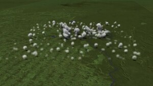
Cumuliform cloudscape
| Forms and levels | Stratiform non-convective | Cirriform mostly non-convective | Stratocumuliform limited-convective | Cumuliform free-convective | Cumulonimbiform strong convective |
|---|---|---|---|---|---|
| Extreme level | Noctilucent (polar mesospheric) | ||||
| Very high level | Polar stratospheric | ||||
| High-level | Cirrostratus | Cirrus | Cirrocumulus | ||
| Mid-level | Altostratus | Altocumulus | |||
| Low-level | Stratus | Stratocumulus | Cumulus humilis | ||
| Multi-level/vertical | Nimbostratus | Cumulus mediocris | |||
| Towering vertical | Cumulus congestus | Cumulonimbus | |||
| Surface-level | Fog |

Etymology and history of cloud science and nomenclature
Etymology
The origin of the term cloud can be found in the old English clud or clod, meaning a hill or a mass of rock. Around the beginning of the 13th century, the word came to be used as a metaphor for rain clouds, because of the similarity in appearance between a mass of rock and cumulus heap cloud. Over time, the metaphoric usage of the word supplanted the old English weolcan, which had been the literal term for clouds in general.
Aristotle and Theophrastus
Ancient cloud studies were not made in isolation, but were observed in combination with other weather elements and even other natural sciences. In about 340 BC the Greek philosopher Aristotle wrote Meteorologica, a work which represented the sum of knowledge of the time about natural science, including weather and climate. For the first time, precipitation and the clouds from which precipitation fell were called meteors, which originate from the Greek word meteoros, meaning 'high in the sky'. From that word came the modern term meteorology, the study of clouds and weather. Meteorologica was based on intuition and simple observation, but not on what is now considered the scientific method. Nevertheless, it was the first known work that attempted to treat a broad range of meteorological topics.[4]
First comprehensive classification
After centuries of speculative theories about the formation and behavior of clouds, the first truly scientific studies were undertaken by Luke Howard in England and Jean-Baptiste Lamarck in France. Howard was a methodical observer with a strong grounding in the Latin language and used his background to classify the various tropospheric cloud types during 1802. He believed that the changing cloud forms in the sky could unlock the key to weather forecasting. Lamarck had worked independently on cloud classification the same year and had come up with a different naming scheme that failed to make an impression even in his home country of France because it used unusual French names for cloud types. His system of nomenclature included twelve categories of clouds, with such names as (translated from French) hazy clouds, dappled clouds and broom-like clouds. By contrast, Howard used universally accepted Latin, which caught on quickly after it was published in 1803.[5] As a sign of the popularity of the naming scheme, the German dramatist and poet Johann Wolfgang von Goethe composed four poems about clouds, dedicating them to Howard. An elaboration of Howard's system was eventually formally adopted by the International Meteorological Conference in 1891.[5] This system covered only the tropospheric cloud types, but the discovery of clouds above the troposphere during the late 19th century eventually led to the creation separate classification schemes for these very high clouds.
Tropospheric
Tropospheric classification is based on a hierarchy of categories with physical forms and altitude levels at the top. These are cross-classified into a total of ten genus types, most of which can be divided into species and further subdivided into varieties which are at the bottom of the hierarchy.
Physical forms
Clouds in the troposphere assume five physical forms based on structure and process of formation. These forms are commonly used for the purpose of satellite analysis.[7] They are given below in approximate ascending order of instability or convective activity.[10]
Stratiform
Non-convective stratiform clouds appear in stable airmass conditions and, in general, have flat sheet-like structures that can form at any altitude in the troposphere.[11] Very low stratiform cloud results when advection fog is lifted above surface level during breezy conditions. The stratiform group is divided by altitude range into the genera cirrostratus (high-level), altostratus (mid-level), stratus (low-level), and nimbostratus (multi-level).[8]
Cirriform
Cirriform clouds are generally of the genus cirrus and have the appearance of detached or semi-merged filaments. They form at high tropospheric altitudes in air that is mostly stable with little or no convective activity, although denser patches may occasionally show buildups caused by limited high-level convection where the air is partly unstable.[12]
Stratocumuliform
Clouds of this structure have both cumuliform and stratiform characteristics in the form of rolls, ripples, or elements.[13] They generally form as a result of limited convection in an otherwise mostly stable airmass topped by an inversion layer.[14] If the inversion layer is absent or higher in the troposphere, increased air mass instability may cause the cloud layers to develop tops in the form of turrets consisting of embedded cumuliform buildups.[15] The stratocumuliform group is divided into cirrocumulus (high-level), altocumulus (mid-level), and stratocumulus (low-level).[13]
Cumuliform
Cumuliform clouds generally appear in isolated heaps or tufts.[16][17] They are the product of localized but generally free-convective lift where there are no inversion layers in the atmosphere to limit vertical growth. In general, small cumuliform clouds tend to indicate comparatively weak instability. Larger cumuliform types are a sign of moderate to strong atmospheric instability and convective activity.[18] Depending on their vertical size, clouds of the cumulus genus type may be low-level or multi-level with moderate to towering vertical extent.
Cumulonimbiform
The largest free-convective clouds comprise the genus cumulonimbus which are multi-level because of their towering vertical extent. They occur in highly unstable air[19] and often have fuzzy outlines at the upper parts of the clouds that sometimes include anvil tops.
Levels and genera

Tropospheric clouds form in any of three levels (formerly called étages) based on altitude range above the Earth's surface. The grouping of clouds into levels is commonly done for the purposes of cloud atlases, surface weather observations[8] and weather maps.[20] The base-height range for each level varies depending on the latitudinal geographical zone.[8] Each altitude level comprises two or three genus types differentiated mainly by physical form.
The standard levels and genus-types are summarised below in approximate descending order of the altitude at which each is normally based.[22] Multi-level clouds with significant vertical extent are separately listed and summarized in approximate ascending order of instability or convective activity.
High-level

High clouds form at altitudes of 3,000 to 7,600 m (10,000 to 25,000 ft) in the polar regions, 5,000 to 12,200 m (16,500 to 40,000 ft) in the temperate regions and 6,100 to 18,300 m (20,000 to 60,000 ft) in the tropics.[8] All cirriform clouds are classified as high and thus constitute a single genus cirrus (Ci). Stratocumuliform and stratiform clouds in the high altitude range carry the prefix cirro-, yielding the respective genus names cirrocumulus (Cc) and cirrostratus (Cs). When limited-resolution satellite images of high clouds are analysed without supporting data from direct human observations, it becomes impossible to distinguish between individual forms or genus types, which are then collectively identified as high-type (or informally as cirrus-type even though not all high clouds are of the cirrus form or genus).[23]
- Genus cirrus (Ci):
- These are mostly fibrous wisps of delicate white cirriform ice crystal cloud that show up clearly against the blue sky.[12] Cirrus are generally non-convective except castellanus and floccus subtypes which show limited convection. They often form along a high altitude jetstream[24] and at the very leading edge of a frontal or low-pressure disturbance where they may merge into cirrostratus. This high-level cloud genus does not produce precipitation.[22]
- Genus cirrocumulus (Cc):

- This is a pure white high stratocumuliform layer of limited convection. It is composed of ice crystals or supercooled water droplets appearing as small unshaded round masses or flakes in groups or lines with ripples like sand on a beach.[25][26] Cirrocumulus occasionally forms alongside cirrus and may be accompanied or replaced by cirrostratus clouds near the leading edge of an active weather system. This genus-type occasionally produces virga, precipitation that evaporates below the base of the cloud.[27]
- Genus cirrostratus (Cs):
- Cirrostratus is a thin non-convective stratiform ice crystal veil that typically gives rise to halos caused by refraction of the sun's rays. The sun and moon are visible in clear outline.[28] Cirrostratus doesn't produce precipitaion, but often thickens into altostratus ahead of a warm front or low-pressure area which sometimes does. [29]
Mid-level
.jpg)
Non-vertical clouds in the middle level are prefixed by alto-, yielding the genus names altocumulus (Ac) for stratocumuliform types and altostratus (As) for stratiform types. These clouds can form as low as 2,000 m (6,500 ft) above surface at any latitude, but may be based as high as 4,000 m (13,000 ft) near the poles, 7,000 m (23,000 ft) at mid latitudes, and 7,600 m (25,000 ft) in the tropics.[8] As with high clouds, the main genus types are easily identified by the human eye, but it is not possible to distinguish between them using satellite photography. Without the support of human observations, these clouds are usually collectively identified as middle-type on satellite images.
- Genus altocumulus (Ac):
- This is a mid-level cloud layer of limited convection that is usually appears in the form of irregular patches or more extensive sheets arranges in groups, lines, or waves.[30] Altocumulus may occasionally resemble cirrocumulus but is usually thicker and composed of a mix of water droplets and ice crystals, so that the bases show at least some light-grey shading.[31] Altocumulus can produce virga, very light precipitation that evaporates before reaching the ground.[32]
- Genus altostratus (As):

- Altostratus is a mid-level opaque or translucent non-convective veil of grey/blue-grey cloud that often forms along warm fronts and around low-pressure areas. Altostratus is usually composed of water droplets but may be mixed with ice crystals at higher altitudes. Widespread opaque altostratus can produce light continuous or intermittent precipitation.
Low-level
Low clouds are found from near surface up to 2,000 m (6,500 ft).[8] Genus types in this level either have no prefix or carry one that refers to a characteristic other than altitude. Clouds that form in the low level of the troposphere are generally of larger structure than those that form in the middle and high levels, so they can usually be identified by their forms and genus types using satellite photography alone.[23]

- Genus stratocumulus (Sc):
- This genus type is a stratocumuliform cloud layer of limited convection, usually in the form of irregular patches or more extensive sheets similar to altocumulus but having larger elements with deeper-gray shading.[34]Stratocumulus is often present during wet weather originating from other rain clouds, but can only produce very light precipitation on its own.[35]
- Genus cumulus (Cu); species humilis – little vertical extent:
- These are small detached fair-weather cumuliform clouds that have nearly horizontal bases and flattened tops, and do not produce rain showers.[36]
- Genus stratus (St):

- This is a flat or sometimes ragged non-convective stratiform type that sometimes resembles elevated fog.[37] Only very weak precipitation can fall from this cloud, usually drizzle or snow grains. When a low stratiform cloud contacts the ground, it is called fog if the prevailing surface visibility is less than 1 kilometer, although radiation and advection types of fog tend to form in clear air rather than from stratus layers.[40] If the visibility increases to 1 kilometer or higher in any kind of fog, the visible condensation is termed mist.
Multi-level (low to mid-level cloud base)

These clouds have low to middle level bases that form anywhere from near surface to about 2,400 m (8,000 ft) and tops that can extend into the high altitude range. Nimbostratus and some cumulus in this group usually achieve moderate or deep vertical extent, but without towering structure. However, with sufficient airmass instability, upward-growing cumuliform clouds can grow to high towering proportions. Although genus types with vertical extent are often informally considered a single group,[42] the International Civil Aviation Organization (ICAO) distinguishes towering vertical clouds more formally as a separate group or sub-group. It is specified that these very large cumuliform and cumulonimbiform types must be identified by their standard names or abbreviations in all aviation observations (METARS) and forecasts (TAFS) to warn pilots of possible severe weather and turbulence.[43] Multi-level clouds are of even larger structure than low clouds, and are therefore identifiable by their forms and genera, (and even species in the case of cumulus congestus) using satellite photography.
- Moderate and deep vertical

- Genus nimbostratus (Ns):
- This is a diffuse dark-grey non-convective stratiform layer with great horizontal extent and moderate to deep vertical development. It lacks towering structure and looks feebly illuminated from the inside.[44] Nimbostratus normally forms from mid-level altostratus, and develops at least moderate vertical extent when the base subsides into the low level during precipitation that can reach moderate to heavy intensity. It commonly achieves deep vertical development when it simultaneously grows upward into the high level due to large scale frontal or cyclonic lift.[46] The nimbo- prefix refers to its ability to produce continuous rain or snow over a wide area, especially ahead of a warm front. This thick cloud layer may be accompanied by embedded towering cumuliform or cumulonimbiform types.Meteorologists affiliated with the World Meteorological Organization (WMO) officially classify nimbostratus as mid-level for synoptic purposes while informally characterizing it as multi-level.[8] Independent meteorologists and educators appear split between those who largely follow the WMO model and those who classify nimbostratus as low-level, despite its considerable vertical extent and its usual initial formation in the middle altitude range.
- Genus cumulus (Cu); species mediocris – moderate vertical extent:
- These cumuliform clouds of free convection have clear-cut medium-grey flat bases and white domed tops in the form of small sproutings and generally do not produce precipitation.[36] They usually form in the low level of the troposphere except during conditions of very low relative humidity when the clouds bases can rise into the middle altitude range. Moderate cumulus is officially classified as low-level and more informally characterized as having vertical extent that can involve more than one altitude level.
- Towering vertical

These clouds are sometimes classified separately from the other vertical or multi-level types because of their ability to produce severe turbulence.
- Genus cumulus (Cu); species congestus – great vertical extent:
- Increasing airmass instability can cause free-convective cumulus to grow very tall to the extent that the vertical height from base to top is greater than the base-width of the cloud. The cloud base takes on a darker grey coloration and the top commonly resembles a cauliflower. This cloud type can produce moderate to heavy showers[36] and is designated Towering cumulus (Tcu) by ICAO.[43]
- Genus cumulonimbus (Cb):

- This genus type is a heavy towering cumulonimbiform mass of free convective cloud with a dark-grey to nearly black base and a very high top in the form of a mountain or huge tower. Cumulonimbus can produce thunderstorms, local very heavy downpours of rain that may cause flash floods, and a variety of types of lightning including cloud-to-ground that can cause wildfires. Other convective severe weather may or may not be associated with thunderstorms and include heavy snow showers, hail, strong wind shear, downbursts, and tornadoes.Of all these possible cumulonimbus-related events, lightning is the only one of these that requires a thunderstorm to be taking place since it is the lightning that creates the thunder. Cumulonimbus clouds can form in unstable airmass conditions, but tend to be more concentrated and intense when they are associated with unstable cold fronts.

Species and varieties

Genus types are commonly divided into subtypes called species that indicate specific structural details which can vary according to the stability and windshear characteristics of the atmosphere at any given time and location. Despite this hierarchy, a particular species may be a subtype of more than one genus, especially if the genera are of the same physical form and are differentiated from each other mainly by altitude or level. There are a few species, each of which can be associated with genera of more than one physical form. The species types are grouped below according to the physical forms and genera with which each is normally associated. The forms, genera, and species are listed in approximate ascending order of instability or convective activity.
Genus and species types are further subdivided into varieties whose names can appear after the species name to provide a fuller description of a cloud. Some cloud varieties are not restricted to a specific altitude level or form, and can therefore be common to more than one genus or species.
Species
Stable or mostly stable Of the stratiform group, high-level cirrostratus comprises two species. Cirrostratus nebulosus has a rather diffuse appearance lacking in structural detail.[59] Cirrostratus fibratus is a species made of semi-merged filaments that are transitional to or from cirrus. Mid-level altostratus and multi-level nimbostratus always have a flat or diffuse appearance and are therefore not subdivided into species. Low stratus is of the species nebulosus[59] except when broken up into ragged sheets of stratus fractus (see below).
Cirriform clouds have three non-convective species that can form in mostly stable airmass conditions. Cirrus fibratus comprise filaments that may be straight, wavy, or occasionally twisted by non-convective wind shear.[60] The species uncinus is similar but has upturned hooks at the ends. Cirrus spissatus appear as opaque patches that can show light grey shading.[57]
Stratocumuliform genus-types (cirrocumulus, altocumulus, and stratocumulus) that appear in mostly stable air have two species each. The stratiformis species normally occur in extensive sheets or in smaller patches where there is only minimal convective activity.[62] Clouds of the lenticularis species tend to have lens-like shapes tapered at the ends. They are most commonly seen as orographic mountain-wave clouds, but can occur anywhere in the troposphere where there is strong wind shear combined with sufficient airmass stability to maintain a generally flat cloud structure. These two species can be found in the high, middle, or low level of the troposphere depending on the stratocumuliform genus or genera present at any given time.
Ragged The species fractus shows variable instability because it can be a subdivision of genus-types of different physical forms that have different stability characteristics. This subtype can be in the form of ragged but mostly stable stratiform sheets (stratus fractus) or small ragged cumuliform heaps with somewhat greater instability (cumulus fractus).[ When clouds of this species are associated with precipitating cloud systems of considerable vertical and sometimes horizontal extent, they are also classified as accessory clouds under the name pannus (see section on supplementary features).[64]
Partly unstable These species are subdivisions of genus types that occur in partly unstable air. The species castellanus appears when a mostly stable stratocumuliform or cirriform layer becomes disturbed by localized areas of airmass instability, usually in the morning or afternoon. This results in the formation of cumuliform buildups arising from a common stratiform base.[65] Castellanus resembles the turrets of a castle when viewed from the side, and can be found with stratocumuliform genera at any tropospheric altitude level and with limited-convective patches of high-level cirrus.[66] Tufted clouds of the more detached floccus species are subdivisions of genus-types which may be cirriform or stratocumuliform in overall structure. They are sometimes seen with cirrus, cirrocumulus, altocumulus, and stratocumulus.[67]
A newly recognized species of stratocumulus or altocumulus has been given the name volutus, a roll cloud that can occur ahead of a cumulonimbus formation.[68] There are some volutus clouds that form as a consequence of interactions with specific geographical features rather than with a parent cloud. Perhaps the strangest geographically specific cloud of this type is the Morning Glory, a rolling cylindrical cloud that appears unpredictably over the Gulf of Carpentaria in Northern Australia. Associated with a powerful "ripple" in the atmosphere, the cloud may be "surfed" in glider aircraft.
Unstable or mostly unstable More general airmass instability in the troposphere tends to produce clouds of the more freely convective cumulus genus type, whose species are mainly indicators of degrees of atmospheric instability and resultant vertical development of the clouds. A cumulus cloud initially forms in the low level of the troposphere as a cloudlet of the species humilis that shows only slight vertical development. If the air becomes more unstable, the cloud tends to grow vertically into the species mediocris, then congestus, the tallest cumulus species[57] which is the same type that the International Civil Aviation Organization refers to as 'towering cumulus'.
With highly unstable atmospheric conditions, large cumulus may continue to grow into cumulonimbus calvus (essentially a very tall congestus cloud that produces thunder), then ultimately into the species capillatus when supercooled water droplets at the top of the cloud turn into ice crystals giving it a cirriform appearance.
Varieties
Opacity-based

All cloud varieties fall into one of two main groups. One group identifies the opacities of particular low and mid-level cloud structures and comprises the varieties translucidus (thin translucent), perlucidus (thick opaque with translucent or very small clear breaks), and opacus (thick opaque). These varieties are always identifiable for cloud genera and species with variable opacity. All three are associated with the stratiformis species of altocumulus and stratocumulus. However, only two varieties are seen with altostratus and stratus nebulosus whose uniform structures prevent the formation of a perlucidus variety. Opacity-based varieties are not applied to high clouds because they are always translucent, or in the case of cirrus spissatus, always opaque.
Pattern-based

A second group describes the occasional arrangements of cloud structures into particular patterns that are discernible by a surface-based observer (cloud fields usually being visible only from a significant altitude above the formations). These varieties are not always present with the genera and species with which they are otherwise associated, but only appear when atmospheric conditions favor their formation. Intortus and vertebratus varieties occur on occasion with cirrus fibratus. They are respectively filaments twisted into irregular shapes, and those that are arranged in fishbone patterns, usually by uneven wind currents that favor the formation of these varieties. The variety radiatus is associated with cloud rows of a particular type that appear to converge at the horizon. It is sometimes seen with the fibratus and uncinus species of cirrus, the stratiformis species of altocumulus and stratocumulus, the mediocris and sometimes humilis species of cumulus, and with the genus altostratus.

Another variety, duplicatus (closely spaced layers of the same type, one above the other), is sometimes found with cirrus of both the fibratus and uncinus species, and with altocumulus and stratocumulus of the species stratiformis and lenticularis. The variety undulatus (having a wavy undulating base) can occur with any clouds of the species stratiformis or lenticularis, and with altostratus. It is only rarely observed with stratus nebulosus. The variety lacunosus is caused by localized downdrafts that create circular holes in the form of a honeycomb or net. It is occasionally seen with cirrocumulus and altocumulus of the species stratiformis, castellanus, and floccus, and with stratocumulus of the species stratiformis and castellanus. Combinations It is possible for some species to show combined varieties at one time, especially if one variety is opacity-based and the other is pattern-based. An example of this would be a layer of altocumulus stratiformis arranged in seemingly converging rows separated by small breaks. The full technical name of a cloud in this configuration would be altocumulus stratiformis radiatus perlucidus, which would identify respectively its genus, species, and two combined varieties.
Accessory clouds, supplementary features, and other derivative types
Supplementary features and accessory clouds are not further subdivisions of cloud types below the species and variety level. Rather, they are either hydrometeors or special cloud types with their own Latin names that form in association with certain cloud genera, species, and varieties. Supplementary features, whether in the form of clouds or precipitation, are directly attached to the main genus-cloud. Accessory clouds, by contrast, are generally detached from the main cloud.[75]
Precipitation-based supplementary features
One group of supplementary features are not actual cloud formations, but precipitation that falls when water droplets or ice crystals that make up visible clouds have grown too heavy to remain aloft. Virga is a feature seen with clouds producing precipitation that evaporates before reaching the ground, these being of the genera cirrocumulus, altocumulus, altostratus, nimbostratus, stratocumulus, cumulus, and cumulonimbus.[75]
When the precipitation reaches the ground without completely evaporating, it is designated as the feature praecipitatio.[76] This normally occurs with altostratus opacus, which can produce widespread but usually light precipitation, and with thicker clouds that show significant vertical development. Of the latter, upward-growing cumulus mediocris produces only isolated light showers, while downward growing nimbostratus is capable of heavier, more extensive precipitation. Towering vertical clouds have the greatest ability to produce intense precipitation events, but these tend to be localized unless organized along fast-moving cold fronts. Showers of moderate to heavy intensity can fall from cumulus congestus clouds. Cumulonimbus, the largest of all cloud genera, has the capacity to produce very heavy showers. Low stratus clouds usually produce only light precipitation, but this always occurs as the feature praecipitatio due to the fact this cloud genus lies too close to the ground to allow for the formation of virga.
Cloud-based supplementary features
Incus is the most type-specific supplementary feature, seen only with cumulonimbus of the species capillatus. A cumulonimbus incus cloud top is one that has spread out into a clear anvil shape as a result of rising air currents hitting the stability layer at the tropopause where the air no longer continues to get colder with increasing altitude.
The mamma feature forms on the bases of clouds as downward-facing bubble-like protuberances caused by localized downdrafts within the cloud. It is also sometimes called mammatus, an earlier version of the term used before a standardization of Latin nomenclature brought about by the World Meterorological Organization during the 20th century. The best-known is cumulonimbus with mammatus, but the mamma feature is also seen occasionally with cirrus, cirrocumulus, altocumulus, altostratus, and stratocumulus.
A tuba feature is a cloud column that may hang from the bottom of a cumulus or cumulonimbus. A newly formed or poorly organized column might be comparatively benign, but can quickly intensify into a funnel cloud or tornado.
An arcus feature is a roll cloud with ragged edges attached to the lower front part of cumulus congestus or cumulonimbus that forms along the leading edge of a squall line or thunderstorm outflow.[80] A large arcus formation can have the appearance of a dark menacing arch.[75]
Several new supplementary features have been formally recognized by the World Meteorological Organization (WMO). The feature fluctus can form under conditions of strong atmospheric wind shear when a stratocumulus, altocumulus, or cirrus cloud breaks into regularly spaced crests. This variant is sometimes known informally as a Kelvin–Helmholtz (wave) cloud. This phenomenon has also been observed in cloud formations over other planets and even in the sun's atmosphere.[81] Another highly disturbed but more chaotic wave-like cloud feature associated with stratocumulus or altocumulus cloud has been given the Latin name asperitas. The supplementary feature cavum is a circular fall-streak hole that occasionally forms in a thin layer of supercooled altocumulus or cirrocumulus. Fall streaks consisting of virga or wisps of cirrus are usually seen beneath the hole as ice crystals fall out to a lower altitude. This type of hole is usually larger than typical lacunosus holes. A murus feature is a cumulonimbus wall cloud with a lowering, rotating cloud base than can lead to the development of tornadoes. A cauda feature is a tail cloud that extends horizontally away from the murus cloud and is the result of air feeding into the storm.
Accessory clouds
Supplementary cloud formations detached from the main cloud are known as accessory clouds. The heavier precipitating clouds, nimbostratus, towering cumulus (cumulus congestus), and cumulonimbus typically see the formation in precipitation of the pannus feature, low ragged clouds of the genera and species cumulus fractus or stratus fractus.[64]
A group of accessory clouds comprise formations that are associated mainly with upward-growing cumuliform and cumulonimbiform clouds of free convection. Pileus is a cap cloud that can form over a cumulonimbus or large cumulus cloud,[82] whereas a velum feature is a thin horizontal sheet that sometimes forms like an apron around the middle or in front of the parent cloud.[75] An accessory cloud recently officially recognized the World meteorological Organization is the flumen, also known more informally as the beaver's tail. It is formed by the warm, humid inflow of a super-cell thunderstorm, and can be mistaken for a tornado. Although the flumen can indicate a tornado risk, it is similar in appearance to pannus or scud clouds and does not rotate.
Mother clouds

Clouds initially form in clear air or become clouds when fog rises above surface level. The genus of a newly formed cloud is determined mainly by air mass characteristics such as stability and moisture content. If these characteristics change over time, the genus tends to change accordingly. When this happens, the original genus is called a mother cloud. If the mother cloud retains much of its original form after the appearance of the new genus, it is termed a genitus cloud. One example of this is stratocumulus cumulogenitus, a stratocumulus cloud formed by the partial spreading of a cumulus type when there is a loss of convective lift. If the mother cloud undergoes a complete change in genus, it is considered to be a mutatus cloud.

Other genitus and mutatus clouds
The genitus and mutatus categories have been expanded to include certain types that do not originate from pre-existing clouds. The term flammagenitus (Latin for 'fire-made') applies to cumulus congestus or cumulonimbus that are formed by large scale fires or volcanic eruptions. Smaller low-level "pyrocumulus" or "fumulus" clouds formed by contained industrial activity are now classified as cumulus homogenitus (Latin for 'man-made'). Contrails formed from the exhaust of aircraft flying in the upper level of the troposphere can persist and spread into formations resembling any of the high cloud genus-types and are now officially designated as cirrus, cirrostratus, or cirrocumulus homogenitus. If a homogenitus cloud of one genus changes to another genus type, it is then termed a homomutatus cloud. Stratus cataractagenitus (Latin for 'cataract-made') are generated by the spray from waterfalls. Silvagenitus (Latin for 'forest-made') is a stratus cloud that forms as water vapor is added to the air above a forest canopy.[68]
Stratocumulus fields[edit]
Stratocumulus clouds can be organized into "fields" that take on certain specially classified shapes and characteristics. In general, these fields are more discernible from high altitudes than from ground level. They can often be found in the following forms:
- Actinoform, which resembles a leaf or a spoked wheel.
- Closed cell, which is cloudy in the center and clear on the edges, similar to a filled honeycomb.[84]
- Open cell, which resembles an empty honeycomb, with clouds around the edges and clear, open space in the middle.
Vortex streets

These patterns are formed from a phenomenon known as a Kármán vortex which is named after the engineer and fluid dynamicist Theodore von Kármán,.[86] Wind driven clouds can form into parallel rows that follow the wind direction. When the wind and clouds encounter high elevation land features such as a vertically prominent islands, they can form eddies around the high land masses that give the clouds a twisted appearance.[87]
Formation and distribution
How air becomes saturated

Air can become saturated as a result of being cooled to its dew point or by having moisture added from an adjacent source. Adiabatic cooling occurs when one or more of three possible lifting agents – cyclonic/frontal, convective, or orographic – causes air containing invisible water vapor to rise and cool to its dew point, the temperature at which the air becomes saturated. The main mechanism behind this process is adiabatic cooling.[88] As the air is cooled to its dew point and becomes saturated, water vapor normally condenses to form cloud drops. This condensation normally occurs on cloud condensation nuclei such as salt or dust particles that are small enough to be held aloft by normal circulation of the air.[19][89]
Frontal and cyclonic lift occur when stable air is forced aloft at weather fronts and around centers of low pressure.[90] Warm fronts associated with extratropical cyclones tend to generate mostly cirriform and stratiform clouds over a wide area unless the approaching warm airmass is unstable, in which case cumulus congestus or cumulonimbus clouds will usually be embedded in the main precipitating cloud layer.[27] Cold fronts are usually faster moving and generate a narrower line of clouds which are mostly stratocumuliform, cumuliform, or cumulonimbiform depending on the stability of the warm air mass just ahead of the front.[56]
Another agent is the convective upward motion of air caused by daytime solar heating at surface level.[19] Airmass instability allows for the formation of cumuliform clouds that can produce showers if the air is sufficiently moist.[91] On moderately rare occasions, convective lift can be powerful enough to penetrate the tropopause and push the cloud top into the stratosphere.[92]
A third source of lift is wind circulation forcing air over a physical barrier such as a mountain (orographic lift).[19] If the air is generally stable, nothing more than lenticular cap clouds will form. However, if the air becomes sufficiently moist and unstable, orographic showers or thunderstorms may appear.[93]

Along with adiabatic cooling that requires a lifting agent, there are three major non-adiabatic mechanisms for lowering the temperature of the air to its dew point. Conductive, radiational, and evaporative cooling require no lifting mechanism and can cause condensation at surface level resulting in the formation of fog.
There are several main sources of water vapor that can be added to the air as a way of achieving saturation without any cooling process: Water or moist ground,precipitation or virga, and transpiration from plants
Convergence along low-pressure zones

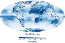
Although the local distribution of clouds can be significantly influenced by topography, the global prevalence of cloud cover tends to vary more by latitude. It is most prevalent globally in and along low pressure zones of surface atmospheric convergence which encircle the Earth close to the equator and near the 50th parallels of latitude in the northern and southern hemispheres.[104] The adiabatic cooling processes that lead to the creation of clouds by way of lifting agents are all associated with convergence; a process that involves the horizontal inflow and accumulation of air at a given location, as well as the rate at which this happens.[105] Near the equator, increased cloudiness is due to the presence of the low-pressure Intertropical Convergence Zone (ITCZ) where very warm and unstable air promotes mostly cumuliform and cumulonimbiform clouds.[106] Clouds of virtually any type can form along the mid-latitude convergence zones depending on the stability and moisture content of the air. These extratropical convergence zones are occupied by the polar fronts where air masses of polar origin meet and clash with those of tropical or subtropical origin.[107] This leads to the formation of weather-making extratropical cyclones composed of cloud systems that may be stable or unstable to varying degrees according to the stability characteristics of the various airmasses that are in conflict.[108]
Divergence along high pressure zones
Divergence is the opposite of convergence. In the Earth's atmosphere, it involves the horizontal outflow of air from the upper part of a rising column of air, or from the lower part of a subsiding column often associated with an area or ridge of high pressure.[105] Cloudiness tends to be least prevalent near the poles and in the subtropics close to the 30th parallels, north and south. The latter are sometimes referred to as the horse latitudes. The presence of a large-scale high-pressure subtropical ridge on each side of the equator reduces cloudiness at these low latitudes.[109] Similar patterns also occur at higher latitudes in both hemispheres.
Luminance, reflectivity, and coloration
The luminance or brightness of a cloud is determined by how light is reflected, scattered, and transmitted by the cloud's particles. Its brightness may also be affected by the presence of haze or photometeors such as halos and rainbows.[111] In the troposphere, dense, deep clouds exhibit a high reflectance (70% to 95%) throughout the visible spectrum. Tiny particles of water are densely packed and sunlight cannot penetrate far into the cloud before it is reflected out, giving a cloud its characteristic white color, especially when viewed from the top.[112] Cloud droplets tend to scatter light efficiently, so that the intensity of the solar radiation decreases with depth into the gases. As a result, the cloud base can vary from a very light to very-dark-grey depending on the cloud's thickness and how much light is being reflected or transmitted back to the observer. High thin tropospheric clouds reflect less light because of the comparatively low concentration of constituent ice crystals or supercooled water droplets which results in a slightly off-white appearance. However, a thick dense ice-crystal cloud appears brilliant white with pronounced grey shading because of its greater reflectivity.[111]
As a tropospheric cloud matures, the dense water droplets may combine to produce larger droplets. If the droplets become too large and heavy to be kept aloft by the air circulation, they will fall from the cloud as rain. By this process of accumulation, the space between droplets becomes increasingly larger, permitting light to penetrate farther into the cloud. If the cloud is sufficiently large and the droplets within are spaced far enough apart, a percentage of the light that enters the cloud is not reflected back out but is absorbed giving the cloud a darker look. A simple example of this is one's being able to see farther in heavy rain than in heavy fog. This process of reflection/absorption is what causes the range of cloud color from white to black.[113]
Striking cloud colorations can be seen at any altitude, with the color of a cloud usually being the same as the incident light.[114] During daytime when the sun is relatively high in the sky, tropospheric clouds generally appear bright white on top with varying shades of grey underneath. Thin clouds may look white or appear to have acquired the color of their environment or background. Red, orange, and pink clouds occur almost entirely at sunrise/sunset and are the result of the scattering of sunlight by the atmosphere. When the sun is just below the horizon, low-level clouds are gray, middle clouds appear rose-colored, and high clouds are white or off-white. Clouds at night are black or dark grey in a moonless sky, or whitish when illuminated by the moon. They may also reflect the colors of large fires, city lights, or auroras that might be present.[114]
A cumulonimbus cloud that appears to have a greenish or bluish tint is a sign that it contains extremely high amounts of water; hail or rain which scatter light in a way that gives the cloud a blue color. A green colorization occurs mostly late in the day when the sun is comparatively low in the sky and the incident sunlight has a reddish tinge that appears green when illuminating a very tall bluish cloud. Supercell type storms are more likely to be characterized by this but any storm can appear this way. Coloration such as this does not directly indicate that it is a severe thunderstorm, it only confirms its potential. Since a green/blue tint signifies copious amounts of water, a strong updraft to support it, high winds from the storm raining out, and wet hail; all elements that improve the chance for it to become severe, can all be inferred from this. In addition, the stronger the updraft is, the more likely the storm is to undergo tornadogenesis and to produce large hail and high winds.
Yellowish clouds may be seen in the troposphere in the late spring through early fall months during forest fire season. The yellow color is due to the presence of pollutants in the smoke. Yellowish clouds are caused by the presence of nitrogen dioxide and are sometimes seen in urban areas with high air pollution levels.


Effects on the atmosphere, climate, and climate change
Clouds exert numerous influences on Earth's atmosphere and climate. First and foremost, they are the source of precipitation, thereby greatly influencing the distribution and amount of precipitation. Because of their differential buoyancy relative to surrounding cloud-free air, clouds can be associated with vertical motions of the air that may be convective, frontal, or cyclonic. The motion is upward if the clouds are less dense because condensation of water vapor releases heat, warming the air and thereby decreasing its density. This can lead to downward motion because lifting of the air results in cooling that increases its density. All of these effects are subtly dependent on the vertical temperature and moisture structure of the atmosphere and result in major redistribution of heat that affect the Earth's climate.
The complexity and diversity of clouds is a major reason for difficulty in quantifying the effects of clouds on climate and climate change. On the one hand, white cloud tops promote cooling of Earth's surface by reflecting shortwave radiation (visible and near infrared) from the sun, diminishing the amount of solar radiation that is absorbed at the surface, enhancing the Earth's albedo. Most of the sunlight that reaches the ground is absorbed, warming the surface, which emits radiation upward at longer, infrared, wavelengths. At these wavelengths, however, water in the clouds acts as an efficient absorber. The water reacts by radiating, also in the infrared, both upward and downward, and the downward longwave radiation results in increased warming at the surface. This is analogous to the greenhouse effect of greenhouse gases and water vapor.
High-level genus-types particularly show this duality with both short-wave albedo cooling and long-wave greenhouse warming effects. On the whole, ice-crystal clouds in the upper troposphere (cirrus) tend to favor net warming. However, the cooling effect is dominant with mid-level and low clouds, especially when they form in extensive sheets. Measurements by NASA indicate that on the whole, the effects of low and mid-level clouds that tend to promote cooling outweigh the warming effects of high layers and the variable outcomes associated with vertically developed clouds.
As difficult as it is to evaluate the influences of current clouds on current climate, it is even more problematic to predict changes in cloud patterns and properties in a future, warmer climate, and the resultant cloud influences on future climate. In a warmer climate more water would enter the atmosphere by evaporation at the surface; as clouds are formed from water vapor, cloudiness would be expected to increase. But in a warmer climate, higher temperatures would tend to evaporate clouds. Both of these statements are considered accurate, and both phenomena, known as cloud feedbacks, are found in climate model calculations. Broadly speaking, if clouds, especially low clouds, increase in a warmer climate, the resultant cooling effect leads to a negative feedback in climate response to increased greenhouse gases. But if low clouds decrease, or if high clouds increase, the feedback is positive. Differing amounts of these feedbacks are the principal reason for differences in climate sensitivities of current global climate models. As a consequence, much research has focused on the response of low and vertical clouds to a changing climate. Leading global models produce quite different results, however, with some showing increasing low clouds and others showing decreases. For these reasons the role of tropospheric clouds in regulating weather and climate remains a leading source of uncertainty in global warming projections.
Above the troposphere
Polar stratospheric

Polar stratospheric clouds show little variation in structure and are limited to a single very high range of altitude of about 15,000–25,000 m (49,200–82,000 ft), so they are not classified into altitude levels, genus types, species, or varieties in the manner of tropospheric clouds.
Polar stratospheric clouds form in the lowest part of the stratosphere during the winter, at the altitude and during the season that produces the coldest temperatures and therefore the best chances of triggering condensation caused by adiabatic cooling. They are typically very thin with an undulating cirriform appearance. Moisture is scarce in the stratosphere, so nacreous and non-nacreous cloud at this altitude range is restricted to polar regions in the winter where the air is coldest.
Polar mesospheric

Polar mesospheric clouds form at a single extreme altitude range of about 80 to 85 km (50 to 53 mi) and are consequently not classified into more than one level. They are given the Latin name noctilucent because of their illumination well after sunset and before sunrise. They typically have a bluish or silvery white coloration that can resemble brightly illuminated cirrus. Noctilucent clouds may occasionally take on more of a red or orange hue.They are not common or widespread enough to have a significant effect on climate. However, an increasing frequency of occurrence of noctilucent clouds since the 19th century may be the result of climate change.
Noctilucent clouds are the highest in the atmosphere and form near the top of the mesosphere at about ten times the altitude of tropospheric high clouds. From ground level, they can occasionally be seen illuminated by the sun during deep twilight. Ongoing research indicates that convective lift in the mesosphere is strong enough during the polar summer to cause adiabatic cooling of small amount of water vapour to the point of saturation. This tends to produce the coldest temperatures in the entire atmosphere just below the mesopause. These conditions result in the best environment for the formation of polar mesospheric clouds. There is also evidence that smoke particles from burnt-up meteors provide much of the condensation nuclei required for the formation of noctilucent cloud.
Distribution in the mesosphere is similar to the stratosphere except at much higher altitudes. Because of the need for maximum cooling of the water vapor to produce noctilucent clouds, their distribution tends to be restricted to polar regions of Earth. A major seasonal difference is that convective lift from below the mesosphere pushes very scarce water vapor to higher colder altitudes required for cloud formation during the respective summer seasons in the northern and southern hemispheres. Sightings are rare more than 45 degrees south of the north pole or north of the south pole.
Extraterrestrial
Cloud cover has been seen on most other planets in the solar system. Venus's thick clouds are composed of sulfur dioxide (due to volcanic activity) and appear to be almost entirely stratiform. They are arranged in three main layers at altitudes of 45 to 65 km that obscure the planet's surface and can produce virga. No embedded cumuliform types have been identified, but broken stratocumuliform wave formations are sometimes seen in the top layer that reveal more continuous layer clouds underneath. On Mars, noctilucent, cirrus, cirrocumulus and stratocumulus composed of water-ice have been detected mostly near the poles. Water-ice fogs have also been detected on Mars.
Both Jupiter and Saturn have an outer cirriform cloud deck composed of ammonia, an intermediate stratiform haze-cloud layer made of ammonium hydrosulfide, and an inner deck of cumulus water clouds.Embedded cumulonimbus are known to exist near the Great Red Spot on Jupiter. The same category-types can be found covering Uranus, and Neptune, but are all composed of methane. Saturn's moon Titan has cirrus clouds believed to be composed largely of methane.The Cassini–Huygens Saturn mission uncovered evidence of polar stratospheric clouds and a methane cycle on Titan, including lakes near the poles and fluvial channels on the surface of the moon.
Some planets outside the solar system are known to have atmospheric clouds. In October 2013, the detection of high altitude optically thick clouds in the atmosphere of exoplanet Kepler-7b was announced, and, in December 2013, in the atmospheres of GJ 436 b and GJ 1214 b.
In culture and religion

Clouds play an important role in various cultures and religious traditions. The ancient Akkadians believed that the clouds were the breasts of the sky goddess Antu and that rain was milk from her breasts. In Exodus 13:21-22, Yahweh is described as guiding the Israelites through the desert in the form of a "pillar of cloud" by day and a "pillar of fire" by night. In the ancient Greek comedy The Clouds, written by Aristophanes and first performed at the City Dionysia in 423 BC, the philosopher Socrates declares that the Clouds are the only true deities[159] and tells the main character Strepsiades not to worship any deities other than the Clouds, but to pay homage to them alone. In the play, the Clouds change shape to reveal the true nature of whoever is looking at them, turning into centaurs at the sight of a long-haired politician, wolves at the sight of the embezzler Simon, deer at the sight of the coward Cleonymus, and mortal women at the sight of the sight of the effeminate informer Cleisthenes. They are hailed the source of inspiration to comic poets and philosophers; they are masters of rhetoric, regarding eloquence and sophistry alike as their "friends". In China, clouds are symbols of luck and happiness.Overlapping clouds are thought to imply eternal happiness and clouds of different colors are said to indicate "multiplied blessings".
The cloud function can be installed at the project level, which is great since I don't want production to have this capability.
It seems that cloud functions are created at the region level and do not have access to zone local IP addresses. As a result, We can't figure out a way to post events to NSQ without exposing it to the public internet.
Cloud Functions lets application developers spin up code on demand in response to events originating from anywhere. Treat all Google and third-party cloud services as building blocks, connect and extend them with code, and build applications that scale from zero to planet-scale—without provisioning or managing a single server.
What you can build with Cloud Functions
erverless application backends
Trigger your code from GCP services or call it directly from any web, mobile, or backend application. Cloud Functions provides a connective layer of logic that lets you integrate and extend GCP and third-party services, making it possible to rapidly build serverless applications that are highly available, secure, and cost-effective.

Integration with third-party services and APIs
Use Cloud Functions to surface your own microservices via HTTP APIs or integrate with third-party services that offer webhook integrations to quickly extend your application with powerful capabilities such as sending a confirmation email after a successful Stripe payment or responding to Twilio text message events.
Example: post a comment on Slack channel in response to a GitHub commit

Serverless mobile backends
Use Cloud Functions directly from Firebase to extend your application functionality without spinning up a server. Run your code code in response to user actions, analytics, and authentication events to keep your users engaged with event-based notifications and offload CPU- and networking-intensive tasks to GCP.
Example: send notifications about new followers

Serverless IoT backends
Use Cloud Functions with Cloud IoT Core and other fully-managed services to build backends for Internet of Things (IoT) device telemetry data collection, real-time processing and analysis. Cloud Functions allows you to apply custom logic to each event as it arrives.
Example: update device configuration
Learn more about Cloud IoT Core

Real-time data processing systems
Execute your code in response to changes in data. Cloud Functions can respond to events from GCP services such as Cloud Storage, Cloud Pub/Sub, and Stackdriver Logging, allowing you to power a variety of serverless real-time data processing systems.

Real-time file processing
Use Cloud Functions to respond to events from Cloud Storage or Firebase Storage to process files immediately after upload to generate thumbnails from image uploads, process logs, validate content, transcode videos, validate, aggregate and filter data in real-time.
Example: image thumbnail generation

Real-time stream processing
Use Cloud Functions to respond to events from Cloud Pub/Sub to process, transform and enrich streaming data in transaction processing, click stream analysis, application activity tracking, IoT device telemetry, social media analysis, and other types of applications.
Example: quality-of-service tracking application


Virtual assistants and conversational experiences
Use Cloud Functions with Google Cloud Speech API and Dialogflow to extend your products and services with voice and text-based natural conversational experiences that help users get things done. Connect with users on the Google Assistant, Amazon Alexa, Facebook Messenger, and other popular platforms and devices.
Video and image analysis
Use Cloud Functions with Google Cloud Video Intelligence API and Cloud Vision API to retrieve relevant information from videos and images, enabling you to search, discover, and derive insight from your media content.
Example: video metadata analysis and extraction
Learn more about

Sentiment Analysis
Use Cloud Functions in combination with Google Natural Language API to reveal the structure and meaning of text and add powerful sentiment analysis and intent extraction capabilities to your applications.
Example: text message sentiment analysis
Learn more about Natural Language API

Microservices over monoliths
Your development agility comes from building systems composed of small, independent units of functionality focused on doing one thing well. Cloud Functions lets you build and deploy services at the level of a single function, not at the level of entire applications, containers, or VMs.
Cloud Functions Overview

What are Google Cloud Functions?
Google Cloud Functions is a serverless execution environment for building and connecting cloud services. With Cloud Functions you write simple, single-purpose functions that are attached to events emitted from your cloud infrastructure and services. Your Cloud Function is triggered when an event being watched is fired. Your code executes in a fully managed environment. There is no need to provision any infrastructure or worry about managing any servers.
Cloud Functions are written in Javascript and execute in a Node.js v6.14.0 environment on Google Cloud Platform. You can take your Cloud Function and run it in any standard Node.js runtime which makes both portability and local testing a breeze.
Connect and Extend Cloud Services
Cloud Functions provides a connective layer of logic that lets you write code to connect and extend cloud services. Listen and respond to a file upload to Cloud Storage, a log change, or an incoming message on a Cloud Pub/Sub topic. Cloud Functions augments existing cloud services and allows you to address an increasing number of use cases with arbitrary programming logic. Cloud Functions have access to the Google Service Account credential and are thus seamlessly authenticated with the majority of Google Cloud Platform services such as Datastore, Cloud Spanner, Cloud Translation API, Cloud Vision API, as well as many others. In addition, Cloud Functions are supported by numerous Node.js client libraries, which further simplify these integrations.
Events and Triggers
Cloud events are things that happen in your cloud environment.These might be things like changes to data in a database, files added to a storage system, or a new virtual machine instance being created.
Events occur whether or not you choose to respond to them. You create a response to an event with a trigger. A trigger is a declaration that you are interested in a certain event or set of events. Binding a function to a trigger allows you to capture and act on events. For more information on creating triggers and associating them with your functions, see Events and Triggers.
Serverless
Cloud Functions removes the work of managing servers, configuring software, updating frameworks, and patching operating systems. The software and infrastructure are fully managed by Google so that you just add code. Furthermore, provisioning of resources happens automatically in response to events. This means that a function can scale from a few invocations a day to many millions of invocations without any work from you.
Use Cases
Asynchronous workloads like lightweight ETL, or cloud automations like triggering application builds now no longer need their own server and a developer to wire it up. You simply deploy a Cloud Function bound to the event you want and you're done.
The fine-grained, on-demand nature of Cloud Functions also makes it a perfect candidate for lightweight APIs and webhooks. In addition, the automatic provisioning of HTTP endpoints when you deploy an HTTP Function means there is no complicated configuration required as there is with some other services. See the following table for additional common Cloud Functions use cases:
| Use Case | Description |
|---|---|
| Data Processing / ETL | Listen and respond to Cloud Storage events such as when a file is created, changed, or removed. Process images, perform video transcoding, validate and transform data, and invoke any service on the Internet from your Cloud Function. |
| Webhooks | Via a simple HTTP trigger, respond to events originating from 3rd party systems like GitHub, Slack, Stripe, or from anywhere that can send HTTP requests. |
| Lightweight APIs | Compose applications from lightweight, loosely coupled bits of logic that are quick to build and that scale instantly. Your functions can be event-driven or invoked directly over HTTP/S. |
| Mobile Backend | Use Google’s mobile platform for app developers, Firebase, and write your mobile backend in Cloud Functions. Listen and respond to events from Firebase Analytics, Realtime Database, Authentication, and Storage. |
| IoT | Imagine tens or hundreds of thousands of devices streaming data into Cloud Pub/Sub, thereby launching Cloud Functions to process, transform and store data. Cloud Functions lets you do it in a way that’s completely server less. |
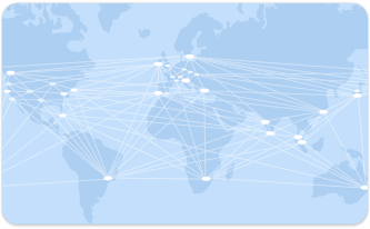
A Fast, High Performance Global Network
Google’s high quality private network connects our regional locations to more than 100 global network points of presence close to your users. Google Cloud Platform also uses state-of-the-art software-defined networkingand distributed systems technologies to host and deliver your services around the world. Google global VPC leverages the Google-owned global high-speed network to link your applications across regions—privately and reliably. When every millisecond of latency counts, Google ensures that your content is delivered with the highest throughput, thanks to innovations like BBR congestion control intelligence.
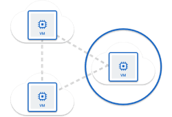
Manage Networking For Your Resources
With Google Virtual Private Cloud (VPC) Network, you can provision your Google Cloud Platform resources, connect them to each other using the Google-owned global network, and isolate them from one another. You can also define fine-grained networking policies with Cloud Platform, on-premise or other public cloud infrastructure. VPC Network is a comprehensive set of Google-managed networking capabilities, including granular IP address range selection, routes, firewall, Virtual Private Network (VPN) and Cloud Router.
Worldwide Autoscaling and Load Balancing
Scale your applications on Google Compute Engine from zero to full-throttle with Google Cloud Load Balancing, with no pre-warming needed. Distribute your load balanced compute resources in single or multiple regions, close to your users and to meet your high availability requirements. Cloud Load Balancing can put your resources behind a single anycast IP and scale your resources up or down with intelligent Autoscaling. Cloud Load Balancing comes in a variety of flavors and is integrated with Google Cloud CDN for optimal application and content delivery.

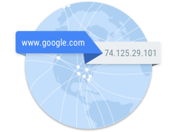
Highly Available Global DNS Network
Google Cloud DNS is a scalable, reliable and managed authoritative Domain Naming System (DNS) service running on the same infrastructure as Google. It has low latency, high availability and is a cost-effective way to make your application and services available to your users. Cloud DNS translates requests for domain names like www.google.com into IP addresses like 74.125.29.101. Cloud DNS is programmable. You can easily publish and manage millions of DNS zones and records using our simple user interface, command-line interface or API.
Fast, High Availability Interconnect
Google Cloud Interconnect allows Cloud platform customers to connect to Google via enterprise-grade connections with higher availability and/or lower latency than their existing Internet connections. Connections are offered by Carrier Interconnect service provider partners, and may offer higher SLAs than standard Internet connections. Google also supports direct connections to its network through direct peering. Customers who cannot meet Google at its peering locations, or do not meet peering requirements, may benefit from Carrier Interconnect.

Content Delivery Network
Google Cloud CDN leverages Google's globally distributed edge caches to accelerate content delivery for websites and applications served out of Google Compute Engine. Cloud CDN lowers network latency, offloads origins, and reduces serving costs. Once you've set up HTTP(S) Load Balancing, simply enable Cloud CDN with a single checkbox.

XO__XO XXX 10001+10 Convenient Driving Components
climate control systems, access systems and other comfort control units but also components for pneumatic seat systems.
Gateway

The Gateway is the network management central electronic control unit, transferring data between various vehicle bus systems. Additionally, the Gateway can be used as a central processing unit, for existing vehicle architecture to be extended with new applications and features.
Features
- Numerous communication interfaces, such as 100BASE-T1Ethernet, 1000BASE-T Ethernet, CAN FD, FlexRay, LIN
- Automotive security through 32bit μC with HW Security
- Functional safety up to ASIL D for routing driver assistance functions
- Latency-free messages routing
Your benefits
- Platform free of intellectual property
- Support of domain based vehicle EE-Architectures
- Time-saving and cost-effective adaptation to individual requirements
- High data security and protection from unauthorised access
- High data rates with ethernet
Climate control

From our extensive expertise in climate control, we can ensure the highest driver and passenger comfort. With manual, semi or fully-automatic control systems, we offer the full range of sophisticated air conditioning solutions including different control systems.
Features
- Climate control as software for integration in your product
- Climate control as integrated solution in Black Box ECU’s
- Climate control in combination with a control unit in a compact design
- Availability of all market-relevant control technologies
- Flexible amount of climate zones within vehicle
- Thermo Management
- Solutions applicable for all known propulsion system
Your benefits
- Flexible and modular SW modules for fast and cost-effective development
- Top-notch climate control for pleasant journeys
Access systems

The modern private and industrial life becomes more and more complex.
There remains no time to deal with unnecessary tasks - such as door closing, key seeking or the electronic devices connection. We develop and supply you with customized solutions for access systems – from the necessary electronics up to keys in your pocket.
There remains no time to deal with unnecessary tasks - such as door closing, key seeking or the electronic devices connection. We develop and supply you with customized solutions for access systems – from the necessary electronics up to keys in your pocket.
Features
- Conventional RF-based access systems (keys and control unit)
- Comfort access via LF and RF systems for vehicle access without keystroke
- Bidirectional access systems for the retrieval of vehicle data on key display or remote vehicle control (parking)
- Access concept via smartphone
- Immobiliser system for securing engine start
- Encrypted communication
Your benefits
- Automatic opening and closing of doors and boot
- Comfortable remote functions and information on key
- High security thanks to encrypted communication technologies
- Appealing, high-quality key design
Body Control Unit (BCU)

The Body Control Unit comprises of all functions in your vehicle, including vehicle lighting, vehicle access, central locking and, for example, wiper control. Using one of our modular kits, we can determine the precise range of functionality of the specific BCU.
Features
- Intelligent interior and light control, indicator signals control
- Access control system
- Wiper control and Rain Sensor
- Immobilizer functions
- Vehicle Power Management
- Gateway functions
- TPMS (Tire Preasure Measurement) Interface
- Numerous communication interfaces, such as CAN, LIN or Ethernet
Your benefits
- Availability of a proven modular platform that allows fast and flexible customisation
Door control unit

The door control unit ensures comfort during the use and control of vehicle doors. Controlling electric windows, locking functions, child locks, functionality of the exterior mirrors, and anti-theft protection features.
Features
- Window control
- Anti-pinch protection with window lifter reversing
- Exterior mirrors control
- Electric child safety locks
- Control of door locks
Your benefits
- Only one central component in the doors
- Optimised cable harness architecture in the doors
- Fewer mechanical and electrical connections required
Seat control unit

The seat control unit ensures comfort during the use and control of vehicle seats. The seat can be adjusted upto twelve directions within seconds. Seat settings can be saved and recalled at any time, vehicle occupants can choose between seat heating and air conditioning.
Features
- Seat control in up to twelve adjustment axes
- Memory function
- Seat heating / seat air conditioning
- Highly accurate positioning
- Anti-pinch protection
Your benefits
- High level of seating comfort for the end customer
- Health promoting thanks to optimal seating positioning
- Personalisation of seating position via the memory function
Pneumatic seat control system

Pneumatic seat systems with massage functions and lumbar support. Individual air cushions are selectively inflated and deflated, seat contours can be dynamically adjusted during rapid cornering, ensuring continued seating position.
Features
- Multi-contour seat for optimum comfort
- Dynamic adjustment of seat contours while cornering
- Low level volume compressors
Your benefits
- High seating comfort for the end customer and for relaxed driving
- Very pleasant seating comfort for passengers in combination with their seat reclining position
- Reduction in back strain (for example, during fast cornering)
- Massage function for the reduction of fatigue levels
Electronic locking systems

Dynamic components in the vehicle can be controlled with electronic locking systems, such as window lifters, sunroofs, convertible rooftops, boot lids and sliding doors.
Features
- Electric car boot actuation (“one touch” activation or in combination with comfort access)
- Speed-controlled operation for smooth opening and closing
- Protection and control algorithms for anti-pinch protection
Your benefits
- High level of comfort for the end customer
- No need to set down luggage before the boot
Smartphone terminal

The Smartphone terminal combines three integrated functions, An inductive charging, NFC communication and wireless antenna coupling for your smartphone.
Features
- Inductive charging for supported devices
- NFC communication for use cases such as personalization or secure BT authentication
- Antenna coupling to reduce smartphone transmission power
Your benefits
- Improved quality of reception signal
- Vehicle HMI personalization via smartphone
- Inductive charging without the hassle of cables or wires in the interior
XO___XO XXX 10001+10 = >2 and <5 Global Circuit Model with Clouds

Cloud data from the International Satellite Cloud Climatology Project (ISCCP) database have been introduced into the global circuit model . Using the cloud-top pressure data and cloud type information, the authors have estimated the cloud thickness for each type of cloud. A treatment of the ion pair concentration in the cloud layer that depends on the radii and concentration of the cloud droplets is used to evaluate the reduction of conductivity in the cloud layer. The conductivities within typical clouds are found to be in the range of 2%–5% of that of cloud-free air at the same altitude, for the range of altitudes for typical low clouds to typical high clouds. The global circuit model was used to determine the increase in columnar resistance of each grid element location for various months in years of high and low volcanic and solar activity, taking into account the observed fractional cloud cover for different cloud types and thickness in each location. For a single 5° × 5° grid element in the Indian Ocean, for example, with the observed fractional cloud cover amounts for low, middle, and high clouds each near 20%, the ionosphere-to-surface column resistance increased by about 10%. (For 100%, fraction—that is, uniformly overcast conditions—for each of the cloud types, the increase depends on the cloud height and thickness and is about a factor of 10 for each of the lower-level clouds in this example and a factor of 2 for the cirrus cloud.) It was found that treating clouds, in the fraction of each grid element in which they were present, as having zero conductivity made very little difference to the results. The increase in global total resistance for the global ensemble of columns in the ionosphere–earth return path in the global circuit was about 10%, applicable to the several solar and volcanic activity conditions, but this is probably an upper limit, in light of the unavailability of data on sub kilometer breaks in cloud cover.
The global atmosphere electric circuit has been postulated, on the basis of a number of sets of correlations, to play a key role in one of the mechanisms by which solar activity affects the earth climate (Tinsley 2000; Tinsley and Yu 2004; Tinsley 2008; Burns et al. 2008). The most important parameter of the global circuit in this mechanism is the ionosphere–surface current density Jz, which varies with changes of the external drivers (space weather); the internal drivers (current output from thunderstorms and other highly electrified clouds); and the distribution of ionosphere–surface column resistance (which depends on ion production from cosmic rays and other energetic particles from the space environment, as well as ionization losses on natural and anthropogenic aerosols). Effects of Jz on cloud microphysics arise because Jz generates space charge in conductivity gradients because of droplet concentration gradients as it passes through clouds, and the space charge puts charges on the order of 10 to 100 elementary charges on aerosol particles and droplets in these gradients (Zhou and Tinsley 2007; Beard et al. 2004). These charges then change the electrically induced scavenging rates in the regions of space charge by up to an order of magnitude (Tinsley et al. 2000, 2001, 2006; Zhou et al. 2009).
The charges can enhance contact ice nucleation rates by increasing the scavenging of relatively large ice-forming nuclei by supercooled droplets, as modeled by Tinsley et al. (2000). Additionally, the charges can increase the scavenging of the large cloud condensation nuclei (CCN) and decrease the phoretic and Brownian scavenging of the smallest CCN (Tinsley 2004; Zhou et al. 2009). Taken with the correlations noted above, which are for meteorological parameters with Jz or proxies for it, the theory and modeling suggests that these electrical enhancements of cloud microphysical processes can account for the observed small changes in regional cloud cover, precipitation, and atmospheric dynamics. The variations of Jz may cause effects on weather and climate from day-to-day time scales up to Milankovich time scales, and observations and theory have been reviewed by Tinsley (2000), Tinsley and Yu (2004), and Tinsley and Zhou (2006).
While effects of Jz on aerosol scavenging affecting their concentration appear to be small compared to other sources of variability in aerosols, the sustained responses to external drivers and to thunderstorm activity changes responding to climate change may be more important. Thus, it is desirable to include in a global circuit model as many as possible of the atmospheric variables that influence Jz. Clouds can affect Jz locally and globally, in addition to Jz having effects on clouds. The conductivity of the air in the cloud layer is reduced because of the attachment of the small air ions to droplets. A small air ion itself is produced by attachment, within a fraction of a second, of several polar molecules to a charged nitrogen or oxygen molecular ion produced by ionizing radiation. Large air ions are produced when the small air ions, in minutes to hours, become large air ions by attachment to aerosol particles. Here we refer to large air ions as charged aerosol particles, in light of the continual interchange between charged and neutral aerosol particles that is implicit in our model.
Measurements and computations (Pruppacher and Klett 1997, section 18.3.2) show that the conductivity in the cloud could be 1/40 to ⅓ of that of the air outside the cloud because of the attachment of small ions to water droplets. The reduction in conductivity increases the columnar resistance R at that location, which reduces Jz there. With clouds over much of the globe increasing the total resistance to the global circuit return current, there can be an increase in ionospheric potential and an increase in Jz in cloud-free areas compared to a totally cloud-free situation. This Jz increase assumes a constant current output of the thunderstorms and highly electrified clouds that are the main generators of the global circuit. A recent discussion of the variability and relative contributions of such generators in different parts of the globe is given by Kartalev et al. (2006).
Since the 1970s, several global circuit models have been constructed, among them those of Hays and Roble (1979), Roble and Hays (1979), Makino and Ogawa (1985), and Sapkota and Varshneya (1990), with the latter two including simple treatments of atmospheric aerosols. In recent work, Tinsley and Zhou (2006) constructed a global circuit model with more accurate treatments of the effects of solar modulation of the cosmic ray flux on the latitude distribution of internal conductivity and the distributions of aerosol in the free troposphere and planetary boundary layer and their seasonal changes, and they made a simple estimate of the effect of ultrafine aerosol production in the stratosphere at high latitudes. The stratospheric ultrafine aerosol particles are formed from H2SO4 vapor resulting from volcanic eruptions, which condenses in the downward branches of the Brewer–Dobson (Garcia and Solomon 1983) circulation. Changes in the cosmic ray flux over a solar cycle were found to affect the global ionosphere-to-surface return path resistance RT by about 7% and changes in stratospheric volcanic aerosols by about 20%. The regional changes were largest at high latitudes, by up to 20% for the solar cycle effect without aerosols, and up to at least a factor of 3 for stratospheric volcanic aerosol effects. Changes in aerosol distributions from July to December increased RT by about 5%.
It is of interest to know if clouds have effects comparable to those of the solar cycle and aerosols. Here, we introduce the cloud cover data from the International Satellite Cloud Climate Project (ISCCP) database into the global circuit model constructed by Tinsley and Zhou (2006) to show the effect on the local column resistances and the global return path resistance of introducing clouds. We also evaluate, for comparison, the effect on the global resistance of introducing aerosols into an aerosol-free atmosphere.
Figure 1 is a schematic circuit diagram representing a half section in the magnetic meridian that includes the dawn–dusk local time plane. The geometry of the global circuit can be treated as plane-parallel because of the large radius of the earth compared to the thickness of the atmosphere. In the model the bottom “plane” is the ground surface, which is equipotential all over the world, and the top plane is the ionosphere effectively at an altitude of 60 km with high conductivity that causes it to be equipotential at latitudes equatorward of about ±60° geomagnetic (gm) latitude. This excludes the geomagnetic polar caps since in the ionospheres of these regions there are additional potential distributions superimposed on the lower-latitude equipotential value due to the interaction among the solar wind, magnetosphere, and ionosphere. The two planes are linked by columns of air that can be treated as independent conductors. The highly electrified convective clouds in three tropical “chimney” regions, the Americas, Africa, and Indonesia–Australia (Williams and Heckman 1993), and in frontal systems and shower clouds at higher latitudes generate upward currents that maintain the potential difference between the ionosphere and the surface. Away from the generator regions the current flows down from the ionosphere to surface, with a current density Jz, which varies with changes of the regional columnar resistance R between ionosphere and surface. The variations of R are due to the effects of geomagnetic latitude on ionizing radiation, as well as to regional changes in the surface altitude, aerosol content and clouds. The circuit diagram in Fig. 1 shows discrete column resistances at equatorial (E), low (L), high (H), and polar (P) latitudes. (The column resistances represent the continuum of conductivity in the conducting atmosphere). In each case a stratospheric columnar resistance S is shown in series with a tropospheric columnar resistance T, although there is no sharp boundary, and there is a continuous variation of conductivity σ(z) over the whole altitude range. Then the total columnar resistance R between the 60-km upper boundary and the surface is given by


The ion pair concentration and mobility, both increasing with height, determine the columnar resistance. The ion pair concentration nf for the steady condition of fair weather (with no cloud) is obtained by the equation

As described by Pruppacher and Klett [1997, section 18.3.2, Eqs. (18)–(37)], who neglected ion–ion recombination and ion attachment to the aerosol, in the weakly electrified cloud in the steady state the ionization rate q is balanced by the loss of ion to droplets at the rate 4πDΣiNiAinc, where D is the ion diffusivity, Ni is the concentration of the cloud droplets with the radius of Ai, and nc is the ion pair concentration in the cloud.
Including this term for ion loss to droplets, the ion pair concentration in the cloud layer in the steady condition, nc, can be obtained by the equation

The ion diffusivity D depends on the ion electrical mobility μ as given by the Einstein formula

We use the variation of mobility with height discussed by Zhou and Tinsley (2007), such that

As in the model made by Tinsley and Zhou (2006), the tropospheric aerosol concentration and size distribution are from the Global Aerosol Dataset (GADS; Hess et al. 1998) and the stratospheric aerosol concentration and size distribution are derived from the simulation made by Yu and Turco (2001). The conductivity for fair weather and within cloud layers can be obtained by the equation

We use the global cloud coverage amount and type data from the International Satellite Cloud Climatology Project D2 database (ISCCP 2004) in which the clouds are divided into three main types (see Fig. 2): low cloud, where the cloud-top pressure is greater than 680 mb, including cumulus, stratocumulus, and stratus; middle cloud, where cloud-top pressure is between 680 and 440 mb, including altocumulus, altostratus, and nimbostratus; and high cloud, with cloud-top pressure between 440 and 50 mb, including cirrus, cirrostratus, and deep convective. The ISCCP D2 dataset is described by Rossow and Schiffer (1999). Deep convective clouds are considered to be the thunderstorm clouds, the generators of the global circuit, and are not included in our model of the resistance of the return path as they occupy only about 2.6% of the globe (Rossow and Schiffer 1999). The fractional coverage of high, middle, and low clouds is highly variable over the globe (this will be illustrated later in Figs. 5a–c and Table 2).
A limitation of the cloud dataset is that there are no entries for cloud cover for night conditions. Thus, there is an absence of entries for high latitudes in the local winters, and the monthly averages of the available data over the rest of the globe are based on daylight conditions. Another limitation of the dataset is that if any cloud is detected in the input data, which has pixel size 4–7 km, it is assumed to fill the whole pixel (Rossow and Schiffer 1999). So clouds which are broken on smaller scales, or which have smaller-scale clear lanes due to downwelling, are treated as being continuous. Preferential flow of electric current density through these small cloud-free (or thin cloud) areas occurs, and there is horizontal spread of current both below and above such breaks in cloud, so that the overall column resistance is overestimated. Another limitation discussed later is in the approximate treatment of cloud-base heights.
The results will show that cloud effects on the global resistance are small compared to aerosol effects; until greater accuracy is available for evaluating aerosol effects and their variability, it is not considered worthwhile to seek greater accuracy in accounting for cloud effects.
Because in general the observations show only partial cloud cover in each 5° × 5° latitude and longitude bin, the equivalent resistivity for each vertical cell of each latitude–longitude bin, r(z), is calculated by the equation

Although the code allows up to 14 different cloud types with their fractional amounts (an ice and a liquid component for three types each of low and middle clouds, and two types of high clouds when deep convective clouds are excluded), we combine fractions of liquid and ice clouds for a maximum of three types at a given level, and a total of eight types.
As in Eq. (1), the columnar resistance R is obtained by

The ISCCP data provide the cloud-top pressure; however, cloud-base pressure is not available at present. So we have to estimate the cloud-base pressure to calculate the depth of the cloud. The definition of the cloud-base height for the ISCCP data follows the method recommended by Ridout and Rosmond (1996), using the Navy Operational Global Atmospheric Prediction System (NOGAPS) hybrid sigma-pressure coordinate system with 18 level grids (Simmons et al. 1989; Hogan and Rosmond 1991). The cirrus, altocumulus, and altostratus clouds are assumed to occupy one grid level, which includes the cloud-top pressure. Cirrostratus clouds are assumed to have a base at 440 mb and nimbostratus clouds are assumed to have a base at the level whose pressure is equal to surface pressure minus 200 mb. The low clouds—cumulus, stratocumulus, and stratus—are assumed to have a base at the level which pressure is equal to surface pressure minus 100 mb. If the calculated base level is above the cloud-top level from ISCCP, the cloud occupies one grid level, which includes the cloud-top pressure. A more accurate value for the increment in column resistance would be obtained by using the approach of Williams et al. (2005) for deriving cloud-base height from air and dewpoint temperatures, but data for utilizing this were not available to us. The pressure as a function of height is obtained by the vertical integration of density obtained from the molecular concentration m of the air, with the following expressions fitted to the values at 0, 10, and 20 km in the U.S. Standard Atmosphere (COESA 1976). The molecular concentration m variation as the function of vertical height is as follows:


The cloud droplet size spectral distribution, ns(r), for the low and middle clouds is from Pruppacher and Klett [1997, Eq. (2.3)]:

The cloud droplet radius is r; the mode radius is rmod; the concentrations of the droplets N for cumulus, stratus, stratocumulus, nimbostratus, and altostratus are from Carrier et al. (1967). Since there is a lack of drop concentration and mode radius data for altocumulus, we assume that its drop concentration and mode radius are the same as for cumulus. We assume that the ice mode has the same particle concentration and mode radius as the liquid mode. This assumption affects the reduction of conductivity in the layer to the extent that the summation ΣiNiAi [from Eq. (4)] is different for the two modes.
The droplet size distribution functions for high clouds follow those of Hess et al. (1998), which are from Heymsfield and Platt (1984) and Liou (1992):


There are four months (July, December, March, and September) within three years of cloud cover data that are used in the global circuit model. Cloud data of 1989 represent the solar maximum and low volcanic activity conditions; the data of 1992, which is one year after the eruption of Pinatubo (1991), represent the high volcanic activity and intermediate solar activity condition; and data of 1996 represent the solar minimum and low volcanic activity condition. It was found by Tinsley and Zhou (2006) that the larger volcanic aerosol particles in the lower stratosphere, although effective in scattering visible light, had a negligible effect on column resistances. However, the ultrafine aerosol production in the downward branches of the Brewer–Dobson circulation at upper-stratospheric levels at high latitudes may double the column resistance there, with effects lasting for 5 years or so. The solar activity effect was found to reach ∼20% at high latitudes, where the relative change in cosmic ray flux is greatest.
a. The variation of the conductivity in the cloud layer
Figures 3a–f show the vertical conductivity variation as a function of altitude for July 1996 at latitude 12.5°S and longitude 92.5°E (which is over the Indian Ocean, with roughly average amounts of cloud cover), with the solid curve indicating the results for no cloud and the dashed, dashed–dotted, and dotted line indicating the results with clouds, assuming 100% cloud cover for low (Figs. 3a,b, with cumulus and stratocumulus), middle (Figs. 3c–e with altocumulus, altostratus, and nimbostratus) and high clouds (Fig. 3f with cirrus), instead of the actual fractional cloud cover for that location and time. In each cloud layer the conductivity greatly decreases (i.e., in low, middle, and high cloud layers the conductivities are ∼1/60 to ∼1/20 that of the cloud-free air at the same level).
b. The effect of the cloud on the columnar resistance and conductivity
Figure 4 shows the vertical conductivity at the grid point for latitude 12.5°S, longitude 92.5°E, for the measured average fraction of the cloud cover for the month of July 1996, where for low clouds the coverage of cumulus is 15.8% and stratocumulus 9.3%; for middle clouds the coverage of altostratus is 9.4%, nimbostratus 5.1%, and altocumulus 0.4%; and for high clouds the coverage of cirrus is 18.6%. The solid curve is the vertical conductivity without cloud and the dashed curve is the vertical conductivity with cloud. The reason for the much smaller effect with partial cloud cover than with the 100% cloud cover in Fig. 3 is that the effective conductivity of the partial cloud layers is now dominated by the (unchanged) high conductivity of the fraction of the clear air (that in this case more than 74%) that remains between the broken clouds. Because of the partial nature of the cloud cover, the conductivity at the cloud level only decreases between 0.1% to 24.2% with the amount of decrease depending on the fraction of the cloud in the bin.
Figures 5a–c show the amount and thickness of low, middle, and high clouds along longitude 92.5°E in July 1996, which is the solar minimum and low volcanic activity year. Cloud data are only available from about 55°S to 90°N owing to polar darkness conditions at high southern latitudes. The choice of the 92.5°E meridian includes a wide variation of surface height over ocean and mountains from the South Pole to the North Pole, with large increases in aerosol concentration in industrial areas, as quantified by Tinsley and Zhou (2006). The increases in elevation decrease the column resistance, while the increases in aerosol concentration increase it. Figure 5d shows the columnar resistance for the same meridian. The solid line is the result without cloud and the dashed line is the result with cloud.
With the partial cloud cover in the column the columnar resistance increases compared to the results with no cloud. Low cloud has a considerably greater effect on column resistance than high cloud because the lower the level in the atmosphere, the lower the conductivity (higher resistivity) of the clear or cloudy air. As can be inferred from Fig. 3 or 4, at 10 km the conductivity is 10 times its value at 2 km, so that a given cloud (of whatever fraction) that increases the resistance of its level by a given factor makes a 10 times greater increment to the ionosphere–surface column resistance if it is at 2 km compared to the increment it would make at 10 km. By way of comparison with the fractional cloud cover results, an evaluation of the effect of 100% cloud fraction for these clouds showed increases that depended on cloud height, thickness, and type, with a factor of about 5–10 for the middle and low clouds considered separately, and a factor of about 2 for the cirrus clouds. These results are shown in Table 1.
Over the Indian Ocean (e.g., 30°S)—with the largest fraction of low cloud, and also high ΣiNiAi, as in Eq. (4), owing to the high liquid water content from warm humid air there—the amount of columnar resistance increase is larger than at any other location (Fig. 5d). Over Asian land the curve with cloud is only slightly higher than that without cloud.
c. Latitude distribution of cloud parameters
Because there is a large variation of different cloud types with latitude, we show in Table 2 zonal averages of cloud properties in 10°-wide latitude increments, as extracted from the ISCCP D2 dataset. Because of the absence of winter polar night data, we show the monthly averages of daytime cloud cover (%) and cloud-top and cloud-base heights (in km) for summer conditions represented by December in the Southern Hemisphere and July in the Northern Hemisphere, respectively. The relatively small amounts of cloud cover, particularly low cloud cover, at high southern latitudes in summer is partly on account of the high altitude of most of the Antarctic continent, with colder and more stable conditions there inhibiting convection, compared to high northern latitudes.
d. Global maps of column resistance
Figures 6a–c show global maps of calculated column resistance for conditions (a) with aerosols but no cloud, (b) with fractional cloud cover from the ISCCP dataset, and (c) with fractional cloud cover as in (b) but with conductivity within clouds set to zero. The Northern Hemisphere is for July 1996 and the Southern Hemisphere is for December 1996. From Fig. 6a we see that without cloud the high-altitude regions in Antarctica, Greenland, and the Himalayas have about an order of magnitude less column resistance (greater column conductance) than oceanic regions at low latitudes, particularly the Pacific, Atlantic, and Indian Oceans. The arid high-altitude regions, and to a lesser extent the low-humidity continental regions that are free from industrial pollution, are largely responsible for the low global ionosphere–earth resistance. This resistance is the reciprocal of the global sum of column conductances (i.e., it is the reciprocal of the global sum of the reciprocals of the column resistances).
Clouds further increase (decrease) the column resistances (conductances) as shown in Figs. 3 to 5, and we see the effects over the globe by comparison of Fig. 6b with Fig. 6a. The changes are relatively small compared to the column resistances without clouds and can be seen in pixel darkening, mostly in middle and high latitudes, and over continents where substantial amounts of clouds are present and column resistances are smaller. There is little effect of clouds in the high-altitude arid regions, especially Antarctica, where this and the relatively high column conductances (which make an important contribution toward the global resistance) ensure a relatively small change in global resistance due to clouds.
There is very little change between Figs. 6b and 6c; only 15 pixels are darkened. This and the later quantitative value show that show that zero conductivity for clouds is a good approximation, in view of the other approximations for the model mentioned earlier.
e. The variation of global resistance RT due to the cloud cover
Table 3 shows the global atmospheric resistance (RT), with the results in columns from left to right for neither aerosols nor cloud cover, for clouds but no aerosol (except for stratospheric aerosol in the lowest two rows), for aerosol but no clouds, and for both clouds and aerosols, shown for conditions with high and low solar and volcanic activity in various combinations for the months of July and December in 1989, 1992, and 1996. These months and years represent the range of seasonal, solar cycle, and volcanic conditions. The same results for no cloud are also given for varying solar activity and volcanic activity conditions in Tinsley and Zhou (2006). The value of global resistance RT with no cloud or aerosol is 113 Ω for the solar minimum period and 117 Ω for the solar maximum period. The lowest two rows in the last three columns represent the addition of stratospheric aerosols for volcanic conditions.
The presence of the tropospheric aerosols generally increases the global resistance by 60%–75%, and the addition of the estimated stratospheric volcanic aerosols brings this increase up to about 90%. The results in the second and fourth data columns show the effect of clouds; while different cloud cover data were used for each of the six periods, there were no significant differences between the percentage changes in RT going from cloud-free to cloudy conditions. Table 3 shows that 1989 is the solar maximum year with low volcanic activity, when RT with clouds is 207 Ω, which is 8.4% higher than that without the clouds; 1992 is the year after volcanic eruption of Pinatubo (1991) with high ultrafine aerosol in the stratosphere at high latitudes and medium solar activity, when RT with cloud reaches 233 Ω, which is 8.4% higher than without clouds; 1996 is the solar minimum year with low volcanic activity, when RT with cloud is 192 Ω, which is 7.9% higher than without clouds. So the model gives cloud enhancements of the global resistance by about 8% in all cases, even for the seasonal variation. The seasonal variation of RT is mainly due to the seasonal variation of the aerosol concentration.
Table 4 is similar to Table 3 except that instead of summer and winter conditions, the results are now for the equinoxes. The results are essentially the same as in Table 3, with again about an 8% increase in RT due to clouds in all cases, with the major increases due to aerosols. The increased coverage of clouds in the southern polar region has had no noticeable effect.
Table 5 gives results for RT for the two hemispheres separately, and for clouds treated as having zero conductivity as well as realistic conductivity. The realistic conductivities are based on the same cloud data that are averaged in Table 2 and are associated with the maps in Fig. 6 (i.e., for July in the NH and December in the SH). The differences between the RT values for the two hemispheres are mainly due to the greater amount of ocean in the Southern Hemisphere. The effect of clouds (about 10%) is slightly higher than the previous results and can be attributed to more convective clouds in summer than in winter. However, as discussed earlier, the cloud effects represent an upper limit, so 10% can be taken as characterizing that upper limit.
The differences between the results for zero cloud conductivity result and the real conductivity is less than 1%. The (unrealistic) combination of results for the two hemispheres gives RT values of 184 Ω for aerosol and no cloud, 202 Ω for aerosol and cloud with real conductivity, and 203 Ω for aerosol and zero cloud conductivity. The small effect of clouds on the global resistance thus contrasts with the 60%–90% effect of aerosols. Thus, the aerosols have about an order of magnitude greater effect than clouds in increasing RT above the value for an aerosol-free and cloud-free atmosphere.
In the cloud layers at a given level with high values of the product ΣiNiAi, as discussed above, high rates of attachment of small air ions to the droplets occur, which causes a large decrease of conductivity in the cloud layer. From models produced by Pluvinage (1946, pp. 31 and 160) and Griffiths et al. (1974), which are in good agreement with measurements (Pruppacher and Klett 1997, section 18.3.2), the conductivity in the cloud layer is typically 1/40 to ⅓ the clear air value at the same level. The condition for the ratio of ⅓ (Allee and Phillips 1959) was for thin clouds and/or open area in clouds of moderate density. Our calculations give the result that within clouds the conductivity is 1/60 to 1/20 of the clear air value (for marine stratus to cirrus). In low-altitude clouds the conductivity is lower than Pluvinage’s value. In the Pluvinage model the concentration of the low cloud droplets was assumed to be 100 cm−3, while the droplet concentration in our model is 3 times higher than Pluvinage’s value. Our more realistic concentration causes greater loss of the ions by attachment to the drops, giving the greater reduction in conductivity.
In each 5° × 5° grid bin the “effective” conductivity at a given level is the average of the relatively high conductivity values for cloud-free air with the relatively low conductivity values for the cloudy air, weighted by the clear and cloud fractions in the bin. For example in Fig. 4, with the 25.1% low cloud in the bin, the conductivity decreases to about three-quarters of the clear air value. The reciprocal of the effective conductivity is the effective resistivity, which is the quantity that is summed in height to give the column resistance as in Eq. (8). Over the Indian Ocean, with the largest amount of thick cloud cover at low altitude (marine cumulus and stratocumulus, as in Fig. 5a), the columnar resistance increase is larger than any other place. Over inland Asia at about 50°N the low amount of low cloud cover and thickness, associated with the downwelling Hadley circulation and desert conditions, causes only a very small increase of the columnar resistance.
The effects of middle and high cloud are smaller than that of low cloud. In Fig. 5 between 20° and 40°N along 92.5°E, although there is about 40% of thick high and about 30% of thick middle cloud cover, the difference of the columnar resistance between the no-cloud condition and the cloud condition is very small. Furthermore, as can be seen in Fig. 5d, the absolute variations in column resistance along the meridian in the cloud-free air that are due to the altitude of the surface and to variations in aerosol content (for details, see Tinsley and Zhou 2006) are much greater than the absolute variation in column resistance due to the cloud cover. Thus, the presence of typical aerosol particle concentrations in the troposphere and ultrafine aerosol particles in the stratosphere has a greater effect on the columnar resistance than that of clouds. This is also shown by comparison with the model results for RT with and without aerosols in Tables 3 and 4.
This model with clouds was developed from the initial global circuit model constructed by Tinsley and Zhou (2006). A treatment to deal with the reduction of conductivity in cloud layers is introduced. With typical low to high cloud layers the conductivity is only 2%–5% of that of cloud-free air at the same level. The inclusion of measured fractional cloud amounts with estimated cloud thickness for each cloud layer can increase the columnar resistance at a given location significantly, by as much as 20% for measured 45% fractional cloud low cloud cover (marine stratocumulus and cumulus). The effect of low cloud on columnar resistance is stronger than that for middle and high cloud. This is because the decreasing resistivity of air with altitude means that a given cloud at high altitude contributes less to the column resistance than if it was at low altitude. The global effects of actual fractional cloud cover on the total ionosphere–earth return path resistance are generally to increase that resistance by an upper limit of about 10% as compared to the larger effect of aerosols, mainly in the continental boundary layer, that increase it by about 60%.
Cloud Types
Cloud Types
Clouds are given different names based on their shape and their height in the sky. Some clouds are near the ground. Others are almost as high as jet planes fly. Some are puffy like cotton. Others are grey and uniform.
The diagram below shows where different types of clouds are located in the sky. Visit the Cloud Gallery to see photos of the different cloud types.

- The highest clouds in the atmosphere are cirrocumulus, cirrus, and cirrostratus. Cumulonimbus clouds can also grow to be very high.
- Mid-level clouds include altocumulus and altostratus.
- The lowest clouds in the atmosphere are stratus, cumulus, and stratocumulus.

Overview of Internet of Things
Internet of Things (IoT) is a sprawling set of technologies and use cases that has no clear, single definition. One workable view frames IoT as the use of network-connected devices, embedded in the physical environment, to improve some existing process or to enable a new scenario not previously possible.
These devices, or things, connect to the network to provide information they gather from the environment through sensors, or to allow other systems to reach out and act on the world through actuators. They could be connected versions of common objects you might already be familiar with, or new and purpose-built devices for functions not yet realized. They could be devices that you own personally and carry with you or keep in your home, or they could be embedded in factory equipment, or part of the fabric of the city you live in. Each of them is able to convert valuable information from the real world into digital data that provides increased visibility into how your users interact with your products, services, or applications.
The specific use cases and opportunities across different industries are numerous, and in many ways the world of IoT is just getting started. What emerges from these scenarios is a set of common challenges and patterns. IoT projects have additional dimensions that increase their complexity when compared to other cloud-centric technology applications, including:
- Diverse hardware
- Diverse operating systems and software on the devices
- Different network gateway requirements
This guide explains the elements you can combine with Google Cloud Platform to build a robust, maintainable, end-to-end IoT solution on Cloud Platform.
Overview of the top-level components
Here we divide the system into three basic components, the device, gateway, and cloud:

A device includes hardware and software that directly interact with the world. Devices connect to a network to communicate with each other, or to centralized applications. Devices might be directly or indirectly connected to the internet.
A gateway enables devices that are not directly connected to the Internet to reach cloud services. Although the term gateway has a specific function in networking, it is also used to describe a class of device that processes data on behalf of a group or cluster of devices. The data from each device is sent to Cloud Platform, where it is processed and combined with data from other devices, and potentially with other business-transactional data.
Types of information
Each device can provide or consume various types of information. Each form of information might best be handled by a different backend system, and each system should be specialized around the data rate, volume, and preferred API. This section lists and describes common categories of information found in IoT scenarios.
Device metadata
Metadata contains information about a device. Most metadata is immutable or rarely changes. Examples of metadata fields include:
- Identifier (ID) - An identifier that uniquely identifies a device. The device ID should never change for the lifespan of a deployed device.
- Class or type
- Model
- Revision
- Date manufactured
- Hardware serial number
State information
State information describes the current status of the device, not of the environment. This information can be read/write. It is updated, but usually not frequently.
Telemetry
Data collected by the device is called telemetry. This is the eyes-and-ears data that IoT devices provide to applications. Telemetry is read-only data about the environment, usually collected through sensors.
Each source of telemetry results in a channel. Telemetry data might be preserved as a stateful variable on the device or in the cloud.
Although each device might send only a single data point every minute, when you multiply that data by a large number of devices, you quickly need to apply big data strategies and patterns.
Commands
Commands are actions performed by a device. Commands often have traits that constrain the choices available in your implementation. These traits include:
- Commands are not easily represented as state data.
- Commands are often not idempotent, which means each duplicate message usually results in a different outcome. Like messaging systems, the implementation of a command function determines the delivery semantics, such as "at least once" or "exactly once". The command mechanism can include a return value, or might rely on the confirmation being made through a separate return message or by reflecting the expected change in the state data.
- Commands might be of limited temporal relevance, so they should include a time-to-live (TTL) or other expiration value.
Examples of commands include:
- Spin 360 degrees to the right.
- Run self cleaning cycle.
- Increase the rate by ten percent.
Operational information
Operational information is data that's most relevant to the operation of the device as opposed to the business application. This might include things such as CPU operating temperature and battery state. This kind of data might not have long-term analytical value, but it has short-term value to help maintain the operating state, such as responding to breakages and correcting performance degradation of software after updates.
Operational information can be transmitted as telemetry or state data.
Devices
It's not always clear what constitutes a device. Many physical things are modular, which means it can be hard to decide whether the whole machine is the device, or each module is a discrete device. There's no single, right answer to this question. As you design your IoT project, you'll need to think about the various levels of abstraction in your design and make decisions about how to represent the physical things and their relationships to each other. The specific requirements of your application will help you understand whether something that generates information should be treated as a device, and therefore deserves its own ID, or is simply a channel or state detail of another device.
As an example, consider a project that has the goal of monitoring the temperature of rooms in a hotel. In each room there might be three sensors: one at the floor by the door, one on the ceiling, and one next to the bed. You can model this setup by representing each sensor as a device:
{deviceID: "dh28dslkja", "location": "floor", "room": 128, "temp": 22 }
{deviceID: "8d3kiuhs8a", "location": "ceiling", "room": 128, "temp": 24 }
{deviceID: "kd8s8hh3o", "location": "bedside", "room": 128, "temp": 23 }
You could also model the entire room as a device. While you usually wouldn't consider a room to be a device, in IoT the device abstraction is really about what you manage and record from as a unit; it isn't always limited to a single gizmo you can hold in your hand. Viewed that way, you could model the hotel room as a device that contains three sensors:
{deviceID: "dh28dslkja", "room": 128, "temp_floor": 22, "temp_ceiling": 24, "temp_bedside": 23, "average_temp": 23 }
Depending on the goals, one of these two data representations might be more correct than the other. Note the average temperature field in the second example. This might be what the hotel is looking for. Is metadata from each sensor most valuable on its own, or do the separate pieces of metadata make more sense applied to the room as a whole? What if the room was a suite and the three locations were the bathroom, lounge, and bedroom? These are the sorts of questions you'd need to ask yourself when deciding how to model the data. The domain model of the connected application defines the exact boundary of what constitutes the device.
Device hardware
General considerations when choosing hardware
When choosing hardware, consider the following factors, which are affected by how the hardware is deployed:
- Cost. Given the value of the data provided, think about what cost can be supported for each device.
- I/O roles. The device might be primarily a sensor, an actuator, or some combination of the two roles.
- Power budget. The device might have access to electricity, or power might be scarce. Think about whether the device will require battery or solar power.
- Networking environment. Consider whether the device can be wired directly to the Internet as TCP/IP routable. Some types of connections, such as cellular, can be expensive with high traffic. Think about the reliability of the network, and the impact of that reliability on latency and throughput. If it is wireless, consider the range the transmission power achieves and the added energy costs.
Functional inputs and outputs
The devices used to interact with the physical world contain components, or are connected to peripherals, that enable sensor input or actuator output. The specific hardware you choose for these hardware I/O components should be based on the functional requirements. For example, the sensitivity or complexity of the motion you need to detect will determine what kind of accelerometer you choose, or whether you need a gyro instead. If you are doing gas detection, the type of gases that the sensor can accurately detect matters. When using a device to produce output, you must consider requirements such as how loud a buzzer needs to sound, how fast a motor needs to turn, or how many amps a relay needs to carry.
In addition to the requirements determined by the environmental performance, the choice of these I/O components or peripherals might also be related to the type of information they are associated with. For example, a stepper motor can be set to a specific direction that might be represented in device state data, while a microphone might be steadily sampling data in terms of frequencies, which is best transmitted as telemetry. These components are connected to the logic systems of the device through a hardware interface.
Device platforms
There is an incredible amount of diversity in the specific hardware available to you for building IoT applications. This diversity starts with the options for hardware platforms. Common examples of platforms include single-board-computers such as the Beaglebone, and Raspberry Pi, as well as microcontroller platforms such as the Arduino series, boards from Particle, and the Adafruit Feather.
Each of these platforms lets you connect multiple types of sensor and actuator modules through a hardware interface.
These platforms interface with the modules using a layered approach similar to those used in general-purpose computing. If you think about the common, everyday computer mouse, you can consider the layers of peripheral, interface, driver and application. On a typical operating system, such as Linux or Windows, the hardware input is interpreted by a driver, which in turn relies on OS services, and might be part of the kernel. For simplicity, the following diagram omits the operating system.

Hardware Interfaces
Most hardware interfaces are serial interfaces. Serial interfaces generally use multiple wires to control the flow and timing of binary information along the primary data wire. Each type of hardware interface defines a method of communicating between a peripheral and the central processor.
IoT hardware platforms use a number of common interfaces. Sensor and actuator modules can support one or more of these interfaces:
- USB. Universal Serial Bus is in common use for a wide array of plug-and-play capable devices.
- GPIO. General-purpose input/output pins are connected directly to the processor. As their name implies, these pins are provided by the manufacturer to enable custom usage scenarios that the manufacturer didn't design for. GPIO pins can be designed to carry digital or analog signals, and digital pins have only two states: HIGH or LOW.Digital GPIO can support Pulse Width Modulation (PWM). PWM lets you very quickly switch a power source on and off, with each "on" phase being a pulse of a particular duration, or width. The effect in the device can be a lower or higher power level. For example, you can use PWM to change the brightness of an LED; the wider the "on" pulses, the brighter the LED glows.Analog pins might have access to an onboard analog-to-digital conversion (ADC) circuit. An ADC periodically samples a continuous, analog waveform, such as an analog audio signal, giving each sample a digital value between zero and one, relative to the system voltage.When you read the value of a digital I/O pin in code, the value must be either HIGH or LOW, where an analog input pin at any given moment could be any value in a range. The range depends on the resolution of the ADC. For example an 8-bit ADC can produce digital values from 0 to 255, while a 10-bit ADC can yield a wider range of values, from 0 to 1024. More values means higher resolution and thus a more faithful digital representation of any given analog signal.The ADC sampling rate determines the frequency range that an ADC can reproduce. A higher sampling rate results in a higher maximum frequency in the digital data. For example, an audio signal sampled at 44,100 Hz produces a digital audio file with a frequency response up to 22.5 kHz, ignoring typical filtering and other processing. The bit precision dictates the resolution of the amplitude of the signal.
- I2C. Inter-Integrated Circuit serial bus uses a protocol that enables multiple modules to be assigned a discrete address on the bus. I2C is sometimes pronounced "I two C", "I-I-C", or "I squared C".
- SPI. Serial Peripheral Interface Bus devices employ a master-slave architecture, with a single master and full-duplex communication. SPI specifies four logic signals:
- SCLK: Serial Clock, which is output from the master
- MOSI: Master Output Slave Input, which is output from the master
- MISO: Master Input Slave Output, which is output from a slave
- SS: Slave Select, which is an active-low signal output from master
- UART. Universal Asynchronous Receiver/Transmitter devices translate data between serial and parallel forms at the point where the data is acted on by the processor. UART is required when serial data must be laid out in memory in a parallel fashion.
Hardware abstraction in software
An operating system abstracts common computing resources such as memory and file I/O. The OS also provides very low-level support for the different hardware interfaces. Generally these abstractions are not easy to use directly, and frequently the OS does not provide abstractions for the wide range of sensor and actuator modules you might encounter in building IoT solutions.
You can take advantage of libraries that abstract hardware interfaces across platforms. These libraries enable you to work with a device, such as a motion detector, in a more straightforward way. Using a library lets you focus on collecting the information the module provides to your application instead of on the low-level details of working directly with hardware.
Some libraries provide abstractions that represent peripherals in the form of lightweight drivers on top of the hardware interfaces. Examples of these libraries include the Johnny-Five JavaScript framework, MRAA, which supports multiple languages, the EMBD Go library, Arduino-wiring, and Firmata.
Computing environment
The computing environment of your platform executes the software. Based on the hardware constraints of power and cost, the capabilities of the processor will vary. Some computing environments consist of a full system on a chip (SOC), which can support an embedded Linux operating system. Microcontroller-based devices might be more constrained, and your application code could run directly on the processor without the support of an operating system.
These computing environments are the bridge between the logic of your application code and the physical hardware of the platform. The software they run might be entirely loaded during boot up from read-only memory (ROM). Alternatively, the environment might result from a staged boot process. This process loads a small program called a bootloader from ROM, which then loads a full operating system from onboard flash or a connected SD card.
On-device processing
After data is collected from a sensor, the device can provide data processing functionality before sending the data to the cloud. Multiple devices might handle the data before it gets to the cloud, and each might perform some amount of processing.
Processing includes things like:
- Converting data to another format
- Packaging data in a way that's secure and combines the data into a practical batch
- Validating data to ensure it meets a set of rules
- Sorting data to create a preferred sequence
- Enhancing data to decorate the core value with additional related information
- Summarizing data to reduce the volume and eliminate unneeded or unwanted detail
- Combining data into aggregate values
On-device analysis can combine multiple processing tasks to provide an intermediate, synthesized interpretation that enables more information to be transmitted in a smaller data footprint.

Device Management
Device management is similar to other IT asset management: the main concerns are provisioning, operating, and updating the devices. These concerns apply to all devices, including gateways.
Provisioning
Provisioning is the process of setting up a new device and making it ready for use. Provisioning includes:
- Bootstrapping with basic device information. At a minimum, a device needs an ID and basic metadata.
- Credentials and authentication required for secure communications. For example, the device can be provided a token or key that can be used for ongoing communications. Such credentials might have an expiration time.
- Authorizing the device. Authorization establishes the permissions of the device to interact with the application or other services, relying on the authentication credentials above. Authorization is the specific permission of the device ID and credential with a specific resource it can use.
- Setting up the network connection. A device needs a network connection to be able to communicate with other services and to transmit data.
- Registering the device. Applications need to know which devices are available. A device registry keeps track of which devices are in use, manages the cloud side of authentication and associates devices with specific data and resources (such as telemetry topics and state storage).
Operations
The daily operation of an IoT system requires that you collect the right information about what's going on. Similar to any IT-hardware deployment, the logging of various events and the monitoring of key status metrics through dashboards and alert mechanisms can help you keep things running smoothly. Cloud Platform provides features that you can use to your advantage for daily operations:
- Stackdriver Logging collects and stores logs. Key device lifecycle events are logged for auditing. A subset of telemetry events can be relayed into Stackdriver Logging for analysis and reporting. Using Stackdriver Logging can save you a lot of time and effort compared to building a custom logging solution.
Over-the-air updates
The sheer scale of a typical IoT deployment means that updating individual devices on site is not practical. Because devices already have some sort of network connection by design, updating devices can be made simpler by pushing updates across the network. In cellular phone parlance, this is an over-the-air (OTA) update, and the same idea applies in IoT. Some options include:
- Android Things. If you use Android-Things-based hardware, OTA updating is built in.
- Setting up your own Debian package repository (APT) on Cloud Platform.
- Resin.io. Based on the Yocto Project, resin.io lets you use familiar tools such as Docker and git to push container image updates.
Gateway
A gateway manages traffic between networks that use different protocols. A gateway is responsible for protocol translation and other interoperability tasks. An IoT gateway device is sometimes employed to provide the connection and translation between devices and the cloud. Because some devices don't contain the network stack required for Internet connectivity, a gateway device acts as a proxy, receiving data from devices and packaging it for transmission over TCP/IP.
A dedicated gateway device might be a requirement if devices in the deployment:
- Don’t have routable connectivity to the Internet, for example, Bluetooth devices.
- Don’t have processing capability needed for transport-layer security (TLS), and as such can't communicate with Google APIs.
- Don't have the electrical power to perform required network transmission.
A gateway device might be used even when the participating devices are capable of communicating without one. In this scenario, the gateway adds value because it provides processing of the data across multiple devices before it is sent to the cloud. In that case, the direct inputs would be other devices, not individual sensors. The following tasks would likely be relegated to a gateway device:
- Condensing data to maximize the amount that can be sent to the cloud over a single link
- Storing data in a local database, and then forwarding it on when the connection to cloud is intermittent
- Providing a real-time clock, with a battery backup, used to provide a consistent timestamp for devices that can't manage timestamps well or keep them well synchronized
- Performing IPV6 to IPV4 translation
- Ingesting and uploading other flat-file-based data from the local network that is relevant and associated with the IoT data
- Acting as a local cache for firmware updates
Cloud Platform
After your IoT project is up and running, many devices will be producing lots of data. You need an efficient, scalable, affordable way to both manage those devices and handle all that information and make it work for you. When it comes to storing, processing, and analyzing data, especially big data, it's hard to beat the cloud.
The following diagram shows the various stages of IoT data management in Cloud Platform:
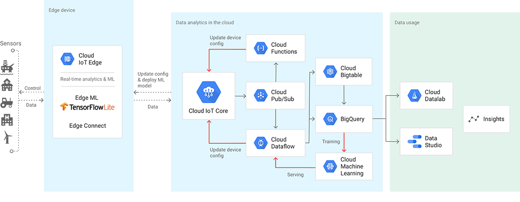
Device Management
IoT Core Device Manager
Google Cloud IoT Core Provides a fully managed service for managing devices. This includes registration, authentication, and authorization inside the Cloud Platform resource hierarchy as well as device metadata stored in the cloud, and the ability to send device configuration from the service to devices.
Ingestion
Ingestion is the process of importing information from devices into Cloud Platform services. Cloud Platform provides different ingestion services, depending on whether the data is telemetry or operational information about the devices and the IoT infrastructure.
IoT Core MQTT
Google Cloud IoT Core Provides a secure MQTT (Message Queue Telemetry Transport) broker for devices managed by IoT Core. This efficient binary industry standard allows for constrained devices to send real-time telemetry as well as immediately receive messages sent from cloud to device by using the configuration management feature. The IoT Core MQTT broker directly connects with Cloud Pub/Sub.
Cloud Pub/Sub
Google Cloud Pub/Sub provides a globally durable message ingestion service. By creating topics for streams or channels, you can enable different components of your application to subscribe to specific streams of data without needing to construct subscriber-specific channels on each device. Cloud Pub/Sub also natively connects to other Cloud Platform services, helping you to connect ingestion, data pipelines, and storage systems.
Cloud Pub/Sub can act like a shock absorber and rate leveller for both incoming data streams and application architecture changes. Many devices have limited ability to store and retry sending telemetry data. Cloud Pub/Sub scales to handle data spikes that can occur when swarms of devices respond to events in the physical world, and buffers these spikes to help isolate them from applications monitoring the data.
Stackdriver Monitoring and Stackdriver Logging
As noted in previous sections, Cloud Monitoring and Stackdriver Logging can provide operational advantages. Operational information is ingested by these services through their provided interfaces.
Pipeline processing tasks
Pipelines manage data after it arrives on Cloud Platform, similar to how parts are managed on a factory line. This includes tasks such as:
- Transforming data. You can convert the data into another format, for example, converting a captured device signal voltage to a calibrated unit measure of temperature.
- Aggregating data and computing. By combining data you can add checks, such as averaging data across multiple devices to avoid acting on a single, spurious, device. You can ensure that you have actionable data if a single device goes offline. By adding computation to your pipeline, you can apply streaming analytics to data while it is still in the processing pipeline.
- Enriching data. You can combine the device-generated data with other metadata about the device, or with other datasets, such as weather or traffic data, for use in subsequent analysis.
- Moving data. You can store the processed data in one or more final storage locations.
Cloud Dataflow
Google Cloud Dataflow provides the open Apache Beam programming model as a managed service for processing data in multiple ways, including batch operations, extract-transform-load (ETL) patterns, and continuous, streaming computation. Cloud Dataflow can be particularly useful for managing the high-volume data processing pipelines required for IoT scenarios. Cloud Dataflow is also designed to integrate seamlessly with the other Cloud Platform services you choose for your pipeline.
Data storage
Data from the physical world comes in various shapes and sizes. Cloud Platform offers a range of storage solutions from unstructured blobs of data, such as images or video streams, to structured entity storage of devices or transactions, and high-performance key-value databases for event and telemetry data.
Storing state in IoT Core
Some device state might be directly connected to the hardware. For example, when you check the state of a digital GPIO pin, it reads as HIGH or LOW, based on the physical reading of the voltage on the pin.
Other device state might exist at the application layer. For example,
recording-audio might have a state condition of true or false, related to whether the application is sampling from the mic or writing to disk. At the hardware level, the mic itself might be left on.
From the software perspective, the application code running on the device maintains the source of truth. It is often valuable, even required, for other software to read the device's last known state. Given that IoT devices can spend some time in low-power sleep mode and might exist on particularly unreliable networks, it's often useful to store some of a device's state in the cloud. That way, state data can be made available even when the devices themselves are temporarily offline.
The last known device state can be reported and stored in IoT Core for retrieval by applications. State information sent over MQTT or HTTP is persisted in IoT Core and is available in the cloud, even if the device has disconnected or gone off line.
Storing application data in Datastore and Firebase
When you need to make state or telemetry data available to mobile or web apps, you can store processed or raw data in structured but schemaless databases, such as Cloud Datastore and Firebase Realtime Database, where you can represent IoT device data as domain or application level objects.
Rule processing and streaming analytics in Cloud Functions and Cloud Dataflow
IoT events and data can be sent to the cloud at a high rate and need to be processed quickly. For many IoT applications, the decision to place the device into the physical environment is made in order to provide faster access to data. For example, produce exposed to high temperatures during shipping can be flagged and disposed of immediately.
Being able to process and act on this information quickly is key. Google Cloud Functions allows you to write custom logic that can be applied to each event as it arrives. This can be used to trigger alerts, filter invalid data, or invoke other APIs. Cloud Functions can operate on each published event individually.
If you need to process data and events with more sophisticated analytics, including time windowing techniques or converging data from multiple streams, Cloud Dataflow provides a highly capable analytics tool that can be applied to streaming and batch data.
Analytics
Performing analytics on data obtained through IoT sources is often the entire purpose of instrumenting the physical world. After streaming data has been analyzed in a processing pipeline, it will begin to accumulate. Over time, this data provides a rich source of information for looking at trends, and can be combined with other data, including data from sources outside of your IoT devices.
BigQuery and Cloud Datalab
Google BigQuery provides a fully managed data warehouse with a familiar SQL interface, so you can store your IoT data alongside any of your other enterprise analytics and logs. The performance and cost of BigQuery means you might keep your valuable data longer, instead of deleting it just to save disk space.
Cloud Datalab is an interactive tool for large-scale data exploration, analysis, and visualization. IoT data can end up being useful for multiple use cases, depending on which other data it's combined with. Cloud Datalab lets you interactively explore, transform, analyze, and visualize your data using a hosted online data workbench environment based on the open source Jupyter project.
Machine Learning
IoT data is often inherently multi-dimensional and noisy by nature. These attributes can make it hard to extract insight by using conventional analytics techniques. However, this nuance and complexity is often where Deep Neural Networks excel. Tensorflow is a leading open source machine learning framework, and on Cloud Platform you can apply Tensorflow in a distributed and managed training service through Cloud Machine Learning Engine.
Time Series dashboards with Cloud Bigtable
Certain types of data need to be quickly sliceable along known indexes and dimensions for updating core visualizations and user interfaces. Cloud Bigtable provides a low-latency and high-throughput database for NoSQL data. Cloud Bigtable provides a good place to drive heavily used visualizations and queries, where the questions are already well understood and you need to absorb or serve at high volumes.
Compared to BigQuery, Cloud Bigtable works better for queries that act on rows or groups of consecutive rows, because Cloud Bigtable stores data by using a row-based format. Compared to Cloud Bigtable, BigQuery is a better choice for queries that require data aggregation.
Archival Storage in Cloud Storage Nearline
The accumulation of data from the world never stops, and the data might not always be structured. Cloud Storageprovides a single API for both current-use object storage, and archival data that is used infrequently. If your IoT device captures media data, Cloud Storage can store virtually unlimited quantities durably and economically.
Conclusion
Building Internet of Things solutions involves solving challenges across a wide range of domains. Cloud Platform brings device management, scale of infrastructure, networking, and a range of storage and analytics products you can use to make the most of device-generated data.
XO___XO XXX 10001+10 = >2 and <5 III III Cloud Detection
The Problem
This project has its roots in a discussion I had a while back with a friend who is a keen amateur astronomer. He had been complaining to me about how he thought that there was a distinct lack of cloud free nights in our corner of Northern Lincolnshire. In fact, he suggested, the weather was so poor that it was hardly worth having a telescope at all.
Okay, so maybe that last sentence was a little exaggeration, but his argument certainly got me thinking - how many clear nights are there in the year? Being a bit of a skeptic, I am sure that the night sky is clear on many more nights than my friend suggests.
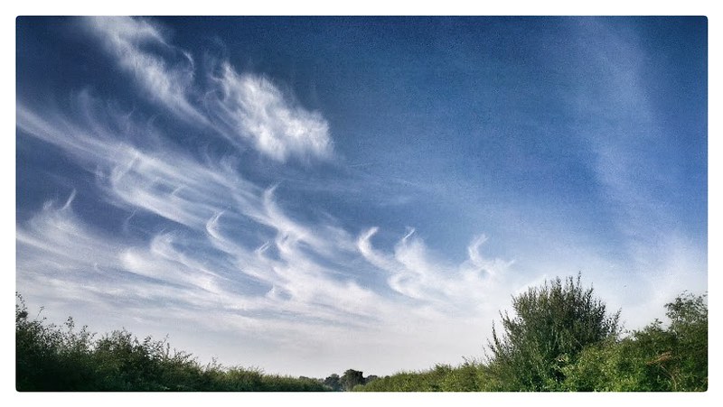
Some clouds, not far from where I live
So this got me thinking - how to measure? Being not only a skeptic, but a lazy skeptic, I wondered how I would be able to count clear nights without having to get up out of bed to go and physically look. There was no way I was going to set alarms at two hourly intervals to find that out. Naturally, the mind turns to remote detection, automation and logging. This sparked off a few days of research into how to measure cloud cover, and took me in many directions; some of which proved to be very interesting. In the end, pretty much all methods for measuring cloud cover come down to one thing - measuring radiated infra red light.
It seems that the easiest way to see how cloudy the sky might be (at night, don't forget), is to look at comparative amounts of infra red light; from the ground and from the sky and then generalise a measurement from there. Essentially, a cloudless sky (whether at night or during the day) radiates less heat than a cloudy one. Compare that to the temperature of the ground under your detector set up and with a lot of calibration and a little bit of luck, you can make a good stab at the level cloud cover.
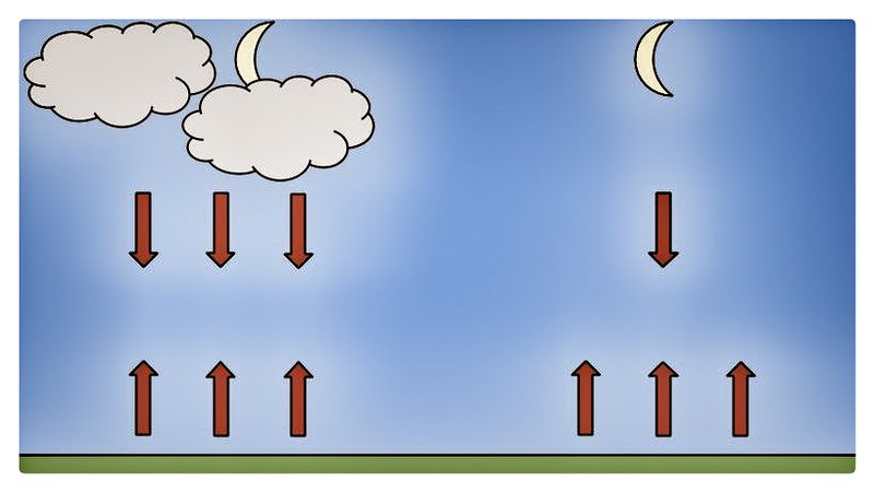
Cloudy versus clear nights and resulting infra red radiation
What about data collection? The measurement method is only half the story, as once measurements are made they will need to be recorded somewhere. It seems to me that the ideal candidate will be an Arduino combined with a way of data retrieval, via serial, ethernet or some other route.
Measurement Methods
During my research I only found two possible methods for comparing ground and sky temperature. All other possibilities were discarded on grounds of cost, my technical (and brain!) limitations, and feasibility.
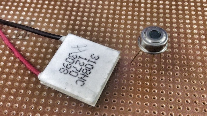
Peltier cooler on the left, MLX90614 sensor on the right
Both methods discussed are based on measuring the difference between sky and ground temperature.
Option One: The Peltier Cooler
According to the Kitt Peak National Observatory web site it is possible to build a thermoelectric sensor based on a device known as a peltier cooler. This detection method utilises the thermoelectric effect whereby a differential of temperature between two surfaces generates a voltage output. This is a reversal of a Peltier cooler's normal use, where a voltage input generates a temperature difference between the two surfaces.
It is therefore supposed a Peltier cooler sandwiched between two isolated aluminium plates, with one plate facing the sky and the other facing the ground, should able to measure the temperature difference between the sky and the ground.
I am assuming that there would have to be some kind of masking set up to ensure that the plates had a view of a measurable area of sky.
Below are some of the advantages and disadvantages of such a system.
Advantages:
- Build costs are relatively cheap; Peltier coolers are readily available at low cost.
- System is reasonably weatherproof; won't require specific protection from the elements.
- The electronics should be fairly simple to put together; just a case of reading analogue output from the sensor.
Disadvantages:
- System will not work well in dewy conditions and does not work at all in the rain.
- Temperature measurement will have to be inferred, as it does not yield an actual temperature reading.
- There exists uncertainty regarding how sensitive the system will be.
- Because of the sensitivity issue, calibration may also be difficult.
Option Two: The Infrared Thermometer - MLX90614 Series
I originally found this MLX series thermometer on the U.S. based Sparkfun site site and was immediately intrigued. The 90614 is a hermetically sealed factory calibrated digital infra red thermometer, packaged in a small TO-39 metal can. They calculate the temperature of the object in view by taking into account the difference between the object and the ambient temperature within the package, measured separately. The cheapest (and most widely available) model has an FoV of 90°. I do have minor concerns that the FoV might be a little too much; testing will tell me all I need to know.
My plan for these thermometers would be to have one unit facing the sky, another unit facing the ground and taking the difference in readings as an approximate measure of cloud cover.
Again, here are some advantages and disadvantages of such a system.
Advantages:
- With higher sensitivity the system should be able to detect more nuanced changes in cloud cover.
- Whilst rain will still stop this system from working, it should not be so badly affected by dew.
- Will yield an actual temperature and won't need much calibration
Disadvantages:
- Build costs are higher than those of the Peltier cooler - the thermometers are more costly and not as easy to get hold of.
- The electronics may be more complex, such as having to deal with I²C busses and so on.
Early Experiments
Before starting on any prototype electronics I thought that I would take some representative measurements of the sky and the ground in different conditions with a digital non-contact thermometer, just to get an idea of the temperature range I might be dealing with here. I got hold of a cheap point and shoot laser type model from my local electronics shop. The thermometer has a digital readout with a range of between -40°C to 365°C, and a (very roughly calculated) field of view (FoV) around 7° when pointed at the sky.
Test Results
Some data output from early tests
It is my belief that neither the MLX or the Peltier (discussed above) will be as sensitive as the thermometer I used in this experiment, for reasons that shall become clear later, therefore the extremes of -40°C should not be experienced in the future.
Onwards
This is the next installment on the cloud detection project. This time I am starting to test out hooking up an MLX90614 or two to an Arduino and try out pointing it to the sky in the aim of get some interesting results.
Just as a friendly warning: calculations done here are rough and ready - don't write to me to say that the cat died because of some experiment based on anything shown here. It's all at your own risk, however, just remember the great Mr Churchill's wise words:
The greatest lesson in life is to know that even fools are right sometimes.
With that in mind, onwards with the experiments...
Field of View
My early experiments, as shown in the first installment were interesting because they showed that IR radiation from even a moderately clear sky would measure well below 0°C; clear skies were regularly below -40°C - out of range on the thermometer. However when testing with the first MLX90614 I bought, I found that the readings were much higher averaging only around -9°C for a clear sky.
I believe that this is mainly due to the field of view of which ever thermometer I was using. I therefore set about making some very simplistic calculations.
Digital Hand Held Thermometer
I calculated the field of view (FOV) of this thermometer to be approximately 7.16°. Compare that with the Sun's angular radius of ~0.5°, then you have a rough idea of how much sky is being covered.
Following that, working out the ratio of viewable sky (r) is not too hard. Being that the field of view is 7.16°, the angular radius (θ) is 3.58°, hence:
which gives us 0.000976 - equivalent to about 1/1025th of the whole sky.
Melexis MLX90614 Family
The MLX90614 family of sensors come in many flavours for a massive range of industrial and medical applications- you can find out absolutely everything you'll ever need to know about these sensors in the datasheet right here. For the rest of this post I am going to look at just two variants.
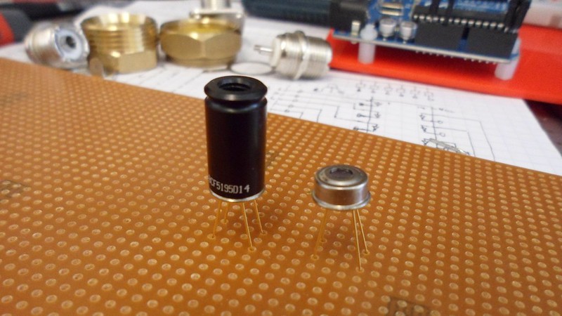
Side by side comparison: BCF on the left, BAA on the right
These sensors sample their ambient temperature as part of the process of measuring infra red object temperature, and as a bonus they make both of these available to the user.
MLX90614 (BAA) Variant
If you were to purchase an MLX90614 from most popular electronics web sites you will more than likely end up with a MLX90614ESF-BAA-000-TU-ND variant in a plain TO-39 package minus fancy lens attachment. Whilst this is probably the cheapest of the MLX90614 family it is also the model with the widest FOV, at a whopping 90° according to the datasheet.
The BAA in the name gives us the option code as described by the datasheet:
- B - 3V supply voltage
- A - Single zone of detection
- A - Standard package (giving the 90° FOV)
The derived θ for this model is 45°, therefore r is 0.146447 giving an equivalent (and rather approximate) view of a massive 1/7th of the sky.
MLX90614 (BCF) Variant
The MLX90614ESF-BCF-000-TU-ND variant of this sensor is a considerably more expensive option; still packaged in a TO-39 case but with a long lens housing. With the price, however, comes a smaller 10° FOV and is built to be more resistant to environmental temperature fluctuations.
Here's what the BCF options give us:
- B - 3V supply voltage
- C - Internal temperature gradient compensation
- F - 10° FOV
The θ for this beast is 5°, with an r value of 0.001903 giving an equivalent view of approximately 1/526th of the sky - very roughly half the value of the digital hand held thermometer.
Hooking up the MLX90614 to an Arduino
Enough of the theory, let's talk about using one.
Connecting to the Arduino
Connecting an MLX90614 to an Arduino is a fairly trivial affair. Looking from the top of the package with the tab at 12 o'clock, there are four legs; clockwise from the tab:
- Ground - connects to any ground on the Arduino.
- Supply - providing you've got the Z3V model, 3.3V on the Arduino is fine.
- SDA - the data line which connects to A4 on the Arduino.
- SCL - the clock line which connects to A5 on the Arduino.
In addition to the above connections a couple of 4k7 pull up resistors are required; one between the SDA line and supply, one between the SCL line and positive. I also like to add a small ceramic capacitor between ground and supply just to stabilise supply voltages a little. You may note that there are two sensors present in the circuit. This presents challenges all of its own, such as how to address more than one sensor in your software. Basically you will need to be able to change the slave address of one of the sensors, as they all come from the manufacturing line with the same address.
I have written up this article here on how to solve that particular problem this article here on how to change the slave address on an MLX90614.
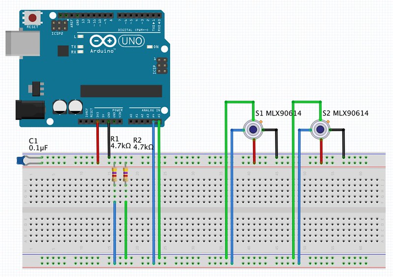
An example of 2 MLX90614 devices and Arduino Uno connected
Software on the Arduino
There aren't a huge number of options for software to get you started on the Arduino; here is just a couple that I found:
- Adafruit have a library here on Github which utilises the Wire library in the background.
- NanoSatisfy host their code on Github which also utilises the Wire library.
I've put together my own library for now which is a slimmed down and lightly modified version of NanoSatisfy's code. Using that, I have written up a quick .ino file which polls both sensors and then outputs a comma separated set of values to the serial port.
Testing the Two Together
After amending the slave address in the BAA variant sensor I assembled the circuit as pictured. I then dug out my 4.8 metre USB lead and placed the Arduino and breadboard in the garden with both sensors side by side, pointing towards an unobstructed view of the night sky. I then uploaded the program and tailed the serial port waiting for data to come in.
Some preliminary test data for both MLX90614 variants
After a couple of hours I turned my log of the serial output into a file, uploaded it to a Google spread sheet and tidied up the presentation a little. Above is a set of 30 sampled results from the test, the samples being taken from the sensors every few minutes.
Conclusion
Below I have graphed a comparison in sky/ground temperature difference between the BAA (blue) and BCF (red) variants, sourced from the test CSV data above. Essentially, the greater the temperature difference between the ground and the sky, the less cloud cover there is.
A graph of both MLX90614 variants compared
It becomes apparent quite quickly that the sensor with the smaller field of view is more responsive to changes in cloud cover, giving a greater dynamic range. This makes sense and was indeed expected, as a sensor's field of view will have a direct relationship with the amount of infra red light it is able to collect from what is, in essence, an infinite distance.
I think that the BAA's ability to see 1/7th of the sky is probably more than what I required for this project. I am only really interested in the sky directly overhead and I think that the BCF will achieve this with the added bonus of better dynamic range.
More testing will be in order, that is for sure, but the indications above seem to me to show that the BCF variant will be the one I will end up using.
Latests Tests
Since the last part in this series I have continued to conduct experiments comparing and contrasting the two variants of MLX90614, the wide field of view BAA and the considerably more focused BCF. Whilst undertaking these 'in the field' tests I have also come up against a few, what you might call, environmental problems which need addressing before I can move from the prototype phase to the implementation phase.
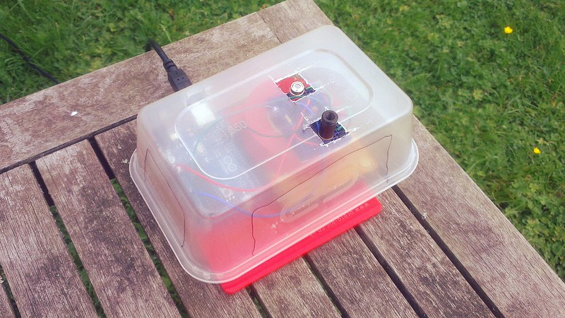
An Arduino has a day out in a box
Environmental Problems
So prototyping electronics within the pleasant warm and dry atmosphere, or 'in the lab' if you prefer, is one thing. However, placing your precious prototype out into the elements is rather another challenge altogether.
Dealing with Dew
One major issue you will come across in these wonderful isles of the United Kingdom if you spend any time in the outdoors at night, particularly in the Autumn months, is high humidity and therefore plenty of dew settling on to surfaces, horizontal ones in particular.
Dew tends to form on surfaces that are at or below a temperature called the dew point. Simply put, there is always water vapour in the air, and if that air is cooled sufficiently the saturation point is reached, which is also called the dew point of the air. Hence the dew point is the temperature at which water vapour in the air will condense on a solid surface. The dew point and air temperature are linked by a property known as relative humidity: the amount of water vapour held in the air.
Relative humidity (RH) from saturation to dry air, is not an absolute scale - at high air temperatures the scale can encompass quite a difference between air and dew point temperatures, say 14°C. At lower air temperatures, near freezing point for example, the scale may only stretch 4°C.
The graph below produced by my weather station illustrates what happens to the relationship between dew point, air temperature and relative humidity over a couple of days.
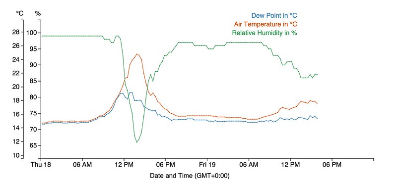
A graph comparing air temperature, dew point and relative humidity
Thankfully, there are a couple lessons which can be learned from the field of amateur observational astronomy; it can be a real battle to keep dew from forming on the mirrors and lenses of telescopes. Essentially there are two countermeasures available against dew in the outdoors: the application of heat or the application of airflow.
- Heat
- One method of preventing dew from forming is to ensure that the object in question is warmed to slightly above the dew point temperature. This is something that is often done with telescope mirrors to prevent them from misting up during the night. You may have seen this sort of thing in hotel rooms where a portion of a bathroom mirror is heated from behind to prevent condensation from forming while you are running the hot taps.
- Airflow
- Introducing a flow of air across an object can also be a successful method of preventing dew from forming, in conditions where the relative humidity is not too high. Bryan Greer mentions, in an article relating to fans on astronomical telescope optics, that"The kinetic energy of the forced airflow makes it harder for seeds of condensation to form"—Bryan GreerPerhaps this may be possible with the inclusion of a small 5 volt fan somewhere near the sensor.
Now these above lessons may be applicable to keeping the sensors clear of moisture. I'm going to have to experiment!
Rain, Rain and more Rain
Another joy of living in these British Isles is the rain. There is rather a lot which for one makes this country fairly green and pleasant, but it does also mean that whatever you do with your precious electronics, you need to make sure that you package them in a decent water resistant package.
MLX90614 are, according to the data sheet, hermetically sealed but what does that actually mean in practice when it comes to dealing with potentially wet environments? The definition of something being hermetically sealed means that it is airtight; this does not mean that the seal is an effective barrier against water.
The data sheet makes no mention of any IP regulation (IP: Ingress Protection) weather proofing so I think that it would be prudent to keep it from the elements in some way. I do not want to have to be replacing these beasts too often as they are not the cheapest of components.
Additionally, whilst the BCF variant of the sensor is fairly flat on the top, the BCF variant has the sensor window in a 20mm well which could potentially fill up with water in a heavy downpour.
In the end I think that this all points to putting the sensor in some sort of housing that will shield it from the weather.
Final Reflection on Rain and Dew
After some thought I have decided that I do not want to leave things to chance: for me there is no question of having the sensor out in the open and pointing to the sky. This leaves only one option which is indirect observation of the sky via a reflective surface, keeping the sensor in the dry and only exposing a mirror of some sort to the sky.
Further Thoughts
This post follows on quite quickly (for me at least!) from my last one regarding my latest tests and reflections on environmental issues with some thoughts about how to measure ground temperatures in a reliable way. I am also going to take a look at the difficulties I might face in trying to automatically interpret cloud cover the whole year through. Finally I am going to share some thoughts on how I might approach packaging the system for deployment in the open air, and what to do about supplying power and communications.
Regarding Temperatures
If there is one thing this project is providing, it is many hours of thought about temperature; both in terms of obtaining measurements that are as accurate as I can make them, and understanding the data that this system will eventually provide.
Measuring Ground Temperature
Initially I started taking ground temperature from the ambient reading given by the MLX90614 sensors. This was just as a matter of quick prototyping to get circuitry outside and gathering test data. It worked well until I packaged the circuit into a plastic box exposed to solar radiation; albeit the lid of the box had two generous squares cut out so that the sensors had access to the sky. Over a few days of data gathering I noticed that the ambient readings being provided by the two MLX90614 variants were consistently higher than the local ground temperature from my weather station and, more importantly, differed from each other by a few degrees Celsius.
It quickly became clear that it was time to find an external way of providing a baseline ground temperature.
A graph comparing ambient measurements taken by the MLX90614 sensors versus a DS18B20
I decided to get a DS18B20 1-wire digital temperature sensor on the scene to in order to provide a baseline from which to see how the two MLX90614 were performing in comparison. The results can be seen in the graph above. It is apparent that indeed sitting a sensor in an small box will not give a very reliable ground temperature reading. In any amount of sunshine the heat inside the box builds very quickly indeed. It is noticeable that the BCF variant gives a reading that is slightly closer to the DS18B20 than the BCC variant. I think that this is probably due to the larger size of the BCF and that it is therefore poking through the cut out in the box lid.
The DS18B20 may not be the only answer: there may be an option to try out pointing a MLX90614 down at the ground; this is, however, something I may have to try at a later date when I get closer to assembling a mark 2 prototype.
Long term I think that measuring ground temperature using an external means such as this will be the only answer to getting accurate measurements down the line. I will be casting my eye over the Met Office surface observations fact sheet in the near future to get more of an idea where I should concentrating my ground temperature measurement efforts.
Interpreting Sky and Ground Temperature
Part of the enjoyment of this project so far has been trying to understand the seasonal variations in temperature of both the sky and the ground. Over years of observing the weather I like to think that, as far as ground temperature goes, I have a pretty good understanding, as would anyone given enough time. However, sky temperature is not something most people take an interest in so it is not surprising that there is little data out there on the subject.
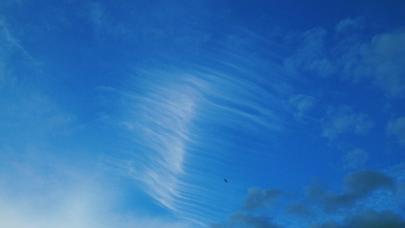
Any excuse to get a cloud photograph in...
In the months so far since I started sampling the sky temperature (which is not quite a year yet), I have seen that a lovely clear blue sky is pretty much at the same temperature on a winters' day as it is at the height of summer; both round about -38°C when measured with my IR thermometer.
Overcast skies tend to differ more between the winter and summer months with those in winter tending to be quite a few degrees colder. This is usually because the cloud base is at or near the same temperature as the ground temperature in the respective season. So a typical summer cloud base temperature might find itself at 12°C; a winter cloud base temperature at -2°C.
In essence the temperature gap between clear skies and cloudy skies is not a straightforward relationship. It depends very much on season and local variation.
Let us look at a simple example:
| Season | Cloud | Sky °C | Ground °C | Gap °C |
|---|---|---|---|---|
| winter | Clear | -38 | -4 | 34 |
| winter | Overcast | -2 | -2 | 0 |
| summer | Clear | -38 | 20 | 58 |
| summer | Overcast | 12 | 14 | 2 |
As of yet I have not firmly planned how I am going to graph the data; I am just aware that having data and making sense of it are two totally different things. It is likely that, at least initially, I will look to just graphing the ground and sky temperatures side by side and leave the interpretation to some manual comparison. Below is an example of such a graph.
Showing both sky and ground temp together; both sensor variants
Ultimately I would love to end up with some sort of heat map with a quarter hour resolution over a 24 hour period. Perhaps this is just mission creep though; the initial idea was just to observe clouds in the night sky. Be that as it may, the ability to do something like this will depend on understanding the temperature limits in the system. All food for thought in the future of this project.
Putting the System Outside
Running a prototype on the bench is nice and simple. There are no concerns with the environmental conditions, other than that your shed is warm, and that there is a cup of tea to hand. Also, there is no concern to the issues with power or communicating with the Arduino; it is all at the end of a USB lead. Of course, this all changes the minute we shift the whole kit outside.
Packaging
When thinking about what type of materials to consider packaging this system in there is only one really sensible answer: plastic. This is because plastic is readily available, easy to work with (in terms of shaping, cutting and bonding), comes in many easy to use shapes and it is relatively cheap. Falling back on experience gained from the soil temperature project I will again look to plastic plumbing supplies for the raw packaging materials. I am also planning to investigate some exterior electrical enclosures, such as weather resistant junction boxes, as a ready made alternative.
Communications
I had originally considered using serial communications but this presented a number of problems, such as what happens as soon as I have more than one Arduino based device collecting data; I am then into the realms of serial networks and so on.
Briefly, I considered using radio of some sort such as Sparkfun's 915MHz wireless transceiver, but then power supply would still be an issue. So my thinking went back to some sort of wired communications. I then came across the marvellous ENC28J60 module which opened up the possibility of using communications over IP - something I am already quite happy with using. The ENC28J60 itself is a fairly self contained 10BASE-T Ethernet controller with a whole host of features including an SPI interface. Here is a data sheet if you are interested.
I won't go into describing how to get an Arduino and ENC28J60 module as there are plenty of articles on the net on how to get started. I will, however, recommend using the UIPEthernet library written by Norbert Truchsess. In my opinion it is by far the best library of the small selection available. It has proven to be very reliable when left running for extended periods, unlike other libraries which have crashed after a few hours.
Power Supply
Once the decision was taken to use wired communications in the form of Ethernet it was but a small light bulb moment to realise that Ethernet does not use all the twisted pairs in a cable; commonly only two of the four available. therefore it seemed to me a no-brainer to use a couple of the spares as a supply and a ground. Being that I am passing DC at a relatively low voltage, I do not anticipate any issues with interference with the network signal.
In Summation
I think that I am closer to coming to a conclusion with the physical build of the project than I am with the interpretation of the data once that starts to flow forth. For now I am just going to concentrate on getting the project built; once I am gathering data the fun is really going to start!
Progress
This post follows on at quite a distance from my last post on the subject, and until recently I had not realised quite how long this project has been languishing on the bench. Like many of the electronics projects I undertake they need to be able to withstand being outside and exposed to weather conditions, dealing with packaging them to handle harsher environments is always the most difficult part.
For the same reason as above, I have also changed one of the key measurement components, the humidity sensor.
I am also dropping the Arduino Uno in favour of the Arduino Yún. I wrote a brief article on the Yún some time ago.
Packaging for the Outdoors
Progress is now being made, finally, on the assembly of the containing hardware of the device. The constituent parts of the detector, namely the box housing for the electronics including the IR detector and the thermostatically controlled heated aluminium mirror have been completed. Now I am in the process of mounting the parts together into a detector assembly. In addition I have made progress on a weather resistant external housing for the entire system to safely be exposed to the elements outside.
Detector Assembly
After thinking about things for a little while, I decided to mount the whole assembly on an acrylic base that will slide in and out of the back of the housing to make maintenance easier. This also keeps the IR detector and mirror at a calibrated distance and angle that should not change between hardware maintenance schedules.
The following photo shows the whole setup:
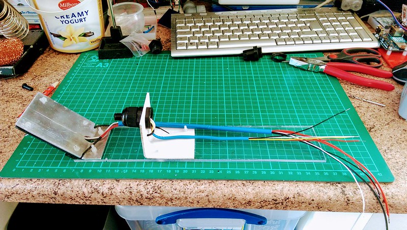
Detector and mirror assembly
The photo below shows the use of a external cable exit gland to hold the IR detector in place. The gland tightens around the plastic housing of the IR detector leaving enough flexibility for fine adjustment if required. The cables have been tidied up using some old heatshrink I had lying around from another project.
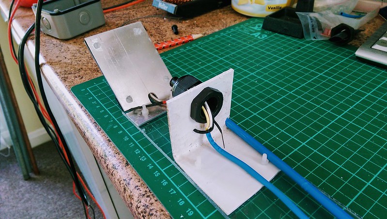
Another view of the detector and mirror assembly
Below you can see the wires exiting from underneath the aluminium mirror. The wires leading from the centre hole at the base go to a DS18B20, a temperature detector, there to measure the surface temperature of the mirror. The black and red wires on the outside edges are connected to heater wires underneath the mirror.
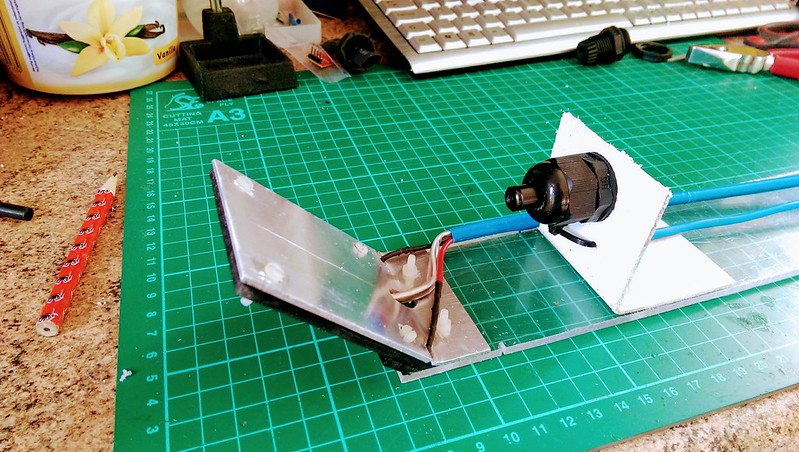
Another view of the detector and mirror assembly
Exterior Housing
Progress is also being made with the exterior housing for the whole setup. The exterior housing (white part) is made from spare 114 mm square section acrylic gutter downpipe. The box (grey) for containing the Arduino and power supplies is an external IP65 rated electrical junction box.
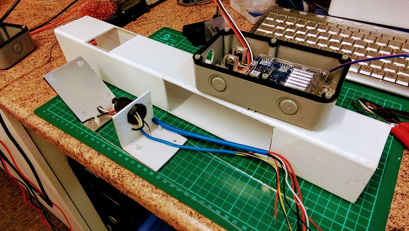
The housing, detector assembly and electronics box
Mirror Heater
The aluminium mirror is the one part of the detector that is exposed to the sky and all that comes from it, be it precipitation, dew and so on. Any form of moisture on the mirror surface will negatively affect the reflectivity. There is not much that can be done about protecting the mirror from the rain, and generally rain means there are clouds. When conditions are clear, meaning no or little cloud, the risk of dew forming on exposed parts is increased. Heating the aluminium gently fixes this problem. Basically, the purpose of the mirror heater is to make sure that the surface of the mirror is maintained a few degrees above dewpoint temperature to ensure that dew does not form on the reflecting surface.
The heater element is to be built from some nichrome wire, commonly found as a heating element in toasters, hairdryers and so on. It is commonly sold in many thicknesses (SWG) and I only need to make sure I calculate the right gauge for the size of heater required.
Calculations
Below is a brief rundown of the calculations required to find what sort of wire was required to build the heater.
Power output
I would like the heater wire to output approximately 0.3 W per cm; being that the wire needs to be approximately 37.5 cm long to cover the mirror back, the total power output will be the following:
Supply Current
Calculating the supply current is quite straightforward. The supply voltage will be 9 V, therefore:
Total Heater Wire Resistance
Now we need to know what the resistance of the entire length of the heater wire will be in order to get the correct gauge nichrome resistance wire:
So the wire ideally needs to have an overall resistance of 6 ohms once built. This includes an extra few centimetres at the end on which to solder on a supply and ground wire.
Let's say that the total length of the wire will be 45.5 cm ; at that length:
Conclusion
Ideally the nichrome resistance wire will need to be rated at . The nearest I could find was 30 SWG (0.315 mm) at , which is what I bought in the end.
Construction
Having scoured eBay for some wire, the first thing I was did a basic test of what I had bought. Placed one test lead of the multimeter at one end of the nichrome resistance wire and ran the other lead along the wire until I got a reading of 6 ohms. That gave a length of about 42 cm. I then dug out some thin heatshrink tubing and cut a length about 8 cm shorter than the wire. Putting the wire through the heatshrink left 4 cm exposed at either end; these ends for attaching to the supply wires.
Probably the most difficult task in putting this heater together was soldering some stranded wire onto each end of the nichrome resistance wire; the metals don't take to each other all that easily. The easiest way turned out to be knotting the wire and supply wire together and then dropping solder onto that.

Rear of mirror exposed with heater element and DS18B20 temperature sensor
Once the supply wires were attached I covered the joints with a little more heatshrink to finish the job off. The picture above shows the heater almost in place with the temperature control sensor alongside.
Operation
There is not much to write about this; the solution is not a novel one!
Thermostatic Control
The basic cycle of thermostatic control for the mirror is set out below:
- Define the hysteresis variable .
- Derive current dew point temperature from a Humidity Sensor .
- Measure the current temperature of the mirror surface .
- Check the state of condition .
If condition 4 is true then apply heat until condition 4 is false. Once condition 4 is true, switch the heat off. is there to ensure that there is a buffer between the dew point and the temperature of the mirror in order to prevent rapid switching of the heater circuit transistor.
Electronics
Control of the heater as above is achieved by using the Arduino to run the thermostatic control cycle, having the DS18B20 to measure and an externally situated HTU21D to measure . Using these inputs the Arduino controls the base voltage of a TIP120 Darlington NPN transistor. This transistor in turn controls the voltage to the heater wire.
Below is a mockup of how to wire up an Arduino to control the base voltage of a transistor thus controlling the higher power supply to the (in this case) coil. Of course, the coil symbol in the diagram represents the heater.
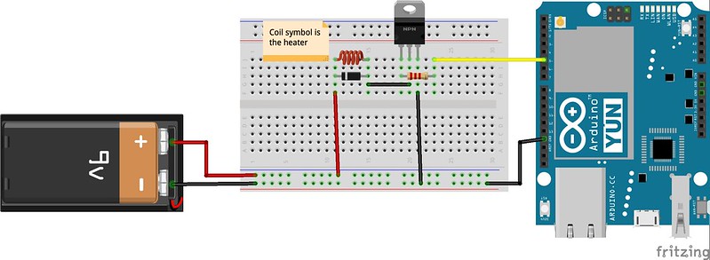
Arduino with TIP120 High Power Control
Humidity Sensor
Sensor Update
I've had some long time concerns about the humidity sensor I had lined up to undertake the task of determining dew point.
Up until recently I had always considered using a DHT22 (also known as an Aosong AM2302) to do the job, but had always been a little unsure of how well adapted this sensor would be to living outside all the time. My uncertainty about their robustness comes mostly from their build quality which, to be polite about it, is not really the best.

DHT22 Humidity Sensor
I suppose that my main concern is how a DHT22 would fare in a cold and wet environment and potentially have its performance degrade leading to short to medium term reliability issues; longer term, I cannot imagine it lasting at all! I could find no satisfactory manufacturer's documentary evidence as to how waterproof the packaging was. There is a good deal of in depth research here comparing the different humidity sensors (or Hygrometers as he calls them) available on the market, for those that are interested in further reading. The DHT22 has an accuracy of around 5% between 0% and 90% humidity. Above 90% humidity the device performance is a little uncertain; no real world data exists, just what is presented in the datasheet. Additionally, Robert from www.kandrsmith.org indicates a 50% device failure rate over a period of 2 years in his research.
So, research into DHT22 alternatives lead me to the HTU21D module.
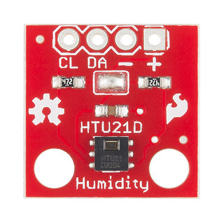
HTU21D Humidity Sensor on a Breakout Board
The stats on the HTU21D look much better; as soon as you take a peek at the datasheet, it becomes obvious that this is a much higher quality product than the DHT series sensor. For a start, there is a proper datasheet rather than the token effort offered by the developers of the DHT22. The build looks much more robust too; both the exterior housing and connector pins are very flimsy on the DHT22, whereas the HTU21D is of a clearly better quality and more robust build.
The HTU21D has a version that comes with a PTFE protector on the sensor window which provides the sensor with a degree of protection from the moisture ingress of an outside environment. Rather than the serial interface of the DHT22, the HTU21D provides I2C communications which I prefer.
Calculating the Dew Point
The dew point temperature measurement is derived from air temperature and humidity both of which are supplied by a humidity sensor. The code I use to derive the dewpoint is written by Rob Tillaart, I cannot even remember when or where I found it, but I have found it useful many times. Below is the code that does the business:
1 2 3 4 5 6 7 8 9 10 11 12 13 14 15 16 17 | double dewPoint(double celsius, double humidity)
{
// (1) Saturation Vapour Pressure = ESGG(T)
double RATIO = 373.15 / (273.15 + celsius);
double RHS = -7.90298 * (RATIO - 1);
RHS += 5.02808 * log10(RATIO);
RHS += -1.3816e-7 * (pow(10, (11.344 * (1 - 1 / RATIO ))) - 1) ;
RHS += 8.1328e-3 * (pow(10, (-3.49149 * (RATIO - 1))) - 1) ;
RHS += log10(1013.246);
// factor -3 is to adjust units - Vapour Pressure SVP * humidity
double VP = pow(10, RHS - 3) * humidity;
// (2) DEWPOINT = F(Vapour Pressure)
double T = log(VP / 0.61078); // temp var
return (241.88 * T) / (17.558 - T);
}
|
Moving from the Uno to the Yún
Over the last year or two I have been experimenting with the Arduino Yún as a replacement for the, ah, mostly reliable Arduino Uno [1]. In the early days I had some interesting times in getting Arduino Unos (and their counterparts) onto my local network, having to resort tosome workarounds to ensure reliability.
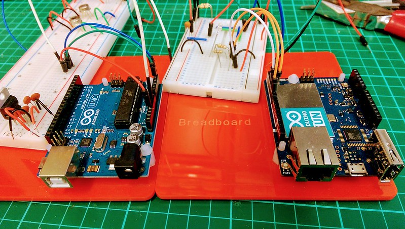
Arduino Uno R3 and Arduino Yún in Comparison
There are a few reasons why I want to move this project over to using a Yún, all of them to do with better reliability and an increased range of functionality. A non-exhaustive list would go something like:
- Much improved networking
- The Yún has built in Ethernet and Wi-Fi support which obviates the need for custom networking hardware and restart handling electronics.
- Better stability
- Over a few months I had the Yún running in a remote situation with real world events taking place, such as swapping out a gateway on the network, power outages (frequent because of where I live!) and so on. I never had any problems getting data from the Yún when I needed to.
- More that just an Arduino
- Of course, the thing that makes the Yún really special is the onboard Linux bridge capabilities that it has. The Atheros AR9331 is basically a Wi-Fi system-on-chip, frequently seen in wireless access points and routers.
The downsides of choosing the Yún are higher initial cost, a more complex architecture and slight incompatibility with some general Arduino libraries.
However, the gain of being able to put an Arduino on the network without breaking any sweat really has me hooked on the Yún. Being that networking comms is taken care of by the addition of the Bridge.h, YunServer.h and YunClient.h libraries, I have an endpoint capable of providing simple and readable RESTful URI resources; something I don't have to even think about programming myself. Because of that, I have the great advantage of more program memory to play with.
Conclusion
So, as can be seen from the collection of things mentioned above, I have moved a long way in getting this project towards completion. It has been a stop / start affair; many other things have intervened and I have had to do some time consuming research. Given the limited free time I have it I do sometimes question whether I will get this finished.
How many volts are in a lightning strike?
we learn that lightning bolts carry from 5 kA to 200 kA and voltages vary from 40 kV to 120 kV. So if we take some averages, say, 100 kA and 100 kV, this bolt would carry this much power, P:
P = 100×103 A x 100 x 103 V
= 10,000 x 106 VA or Watts
= 1 x 10¹⁰ Watts
Recall that 1010 Watts is 10,000,000,000 or 10 billion Watts.
Now assume this energy is released in 1 sec. So the power is:
1010 W-sec. On your electric bill, you’ll see you pay for Watt-hours or Wh. So let’s convert W-sec to Wh:
Pl = 1010 Ws x 1 hr/3600 s
Pl = 1/36 x 108 Wh
= 0.0277 x 108
= 2.7 x 10⁶ Wh or Watt-hour per our average lightning bolt.
But can that power a town? And if so, for how long?
How much power does a single house consume? Again we have to play with averages. So let’s assume one house needs 2,000 Watts/hour to keep the frig, furnace, computer, and all things plugged in going. In one day, 24 hours, the house consumes
Ph = 2,000 Watts x 24 hr.
= 48,000 Wh
So if we divide the power draw for the house into the power of a lightning bolt, we’ll have the number of houses that bolt can power:
N = 2.7 x 10⁶ Wh per bolt / 4.8 x 10⁴ Wh/house
= 0.5625 x 102
= 56 houses/bolt of lightning for one day. So the answer to the original question is that a big bolt could power a small, 56-house town for a day.
That assumes we can catch all of that average bolt of lightning in a large capacitor. If you assume a capture efficiency, that would add a few more calculations. Still, the original question is intriguing.
If you wish to take this math experiment a step further, consider how often the U.S. is struck with lightning each day. NOAA online says 22 million cloud-to-ground strikes per year.
Why can't we extract electricity from lightning?
From purely electrical charge calculations:
1. Each lightning strike has on average only five billion joules, that is equivalent to only around 1,400kWh of energy if we assume zero loss in transfer and storage.
2. Lightning strikes over a year are around 1.4 billion, and of those, only about 25 per cent are actually ground strikes since most (75 per cent) are intra-cloud and cloud-cloud, and cannot be harnessed. That leaves only 350 million lightning strikes that could possibly be harnessed. Also, assuming 100 per cent harnessing of all lightning strikes, no loss in capture, transfer and storage, that is 490,000,000,000kWh/year.
3. In 2009, the world used around 20,279,640,000,000kWh – over 40 times the electrical energy that all the hypothetically harness-able land strikes contain. So, basically, all the lightning we can capture will give the world enough electricity for only nine days!
But there is more. If you want to see how much it would cost to do that:
To capture each and every lightning strike (land strikes only) we would most likely have to put extremely tall towers (think the Eiffel Tower) around a mile apart in a grid formation covering the entire globe. That is one tower for each of the almost 200,000,000sq m of the Earth's surface.
The equipment to capture the electrical energy in a strike would have to handle the extreme amount of charge in only around 30 milliseconds (approximate duration of a lighting strike). To handle that kind of instantaneous power, heavy conduction rods would need to be used, with ultra-heavy-duty electrical circuits and storage super-capacitors.
Although we do not have that technology in electrical energy storage yet, let's assume we do, and let's also assume that the energy system is 100 per cent efficient (understanding that most electrical systems when working optimally are less than 70-80 per cent efficient at best), then we can imagine a cost for each tower and electrical circuitry storage would be around £350,000. That is £67 trillion for the land equipment only, ie, with no flotation device for ocean and sea versions. Not to mention installation costs and regular maintenance, as well as the wire grid connecting all the towers together, and the havoc that will cause with air traffic... More money than the world has!
In comparison, one hour of sunlight has the same amount of energy that we use in a year! We have much more power available from the sun and we only need our rooftops to accumulate all we need.
Also lightning and lightning have the speed of contents and exhaust electrical energy very quickly and no media or electronic storage material ready to quickly accommodate electrical energy in lightning and lightning .
Capacitors : devices for storing charge
Capacitors
A capacitor is a device for storing charge. It is usually made up of two plates separated by a thin insulating material known as the dielectric. One plate of the capacitor is positively charged, while the other has negative charge.
The charge stored in a capacitor is proportional to the potential difference between the two plates. For a capacitor with charge Q on the positive plate and -Q on the negative plate, the charge is proportional to the potential:
If C is the capacitance, Q = CV
The capacitance is a measure of the amount of charge a capacitor can store; this is determined by the capacitor geometry and by the kind of dielectric between the plates. For a parallel plate capacitor made up of two plates of area A and separated by a distance d, with no dielectric material, the capacitance is given by :

Note that capacitance has units of farads (F). A 1 F capacitor is exceptionally large; typical capacitors have capacitances in the pF - microfarad range.
Dielectrics, insulating materials placed between the plates of a capacitor, cause the electric field inside the capacitor to be reduced for the same amount of charge on the plates. This is because the molecules of the dielectric material get polarized in the field, and they align themselves in a way that sets up another field inside the dielectric opposite to the field from the capacitor plates. The dielectric constant is the ratio of the electric field without the dielectric to the field with the dielectric:

Note that for a set of parallel plates, the electric field between the plates is related to the potential difference by the equation:
for a parallel-plate capacitor: E = V / d
For a given potential difference (i.e., for a given voltage), the higher the dielectric constant, the more charge can be stored in the capacitor. For a parallel-plate capacitor with a dielectric between the plates, the capacitance is:

Energy stored in a capacitor
The energy stored in a capacitor is the same as the work needed to build up the charge on the plates. As the charge increases, the harder it is to add more. Potential energy is the charge multiplied by the potential, and as the charge builds up the potential does too. If the potential difference between the two plates is V at the end of the process, and 0 at the start, the average potential is V / 2. Multiplying this average potential by the charge gives the potential energy : PE = 1/2 Q V.
Substituting in for Q, Q = CV, gives:
The energy stored in a capacitor is: U = 1/2 C V2
Capacitors have a variety of uses because there are many applications that involve storing charge. A good example is computer memory, but capacitors are found in all sorts of electrical circuits, and are often used to minimize voltage fluctuations. Another application is a flash bulb for a camera, which requires a lot of charge to be transferred in a short time. Batteries are good at providing a small amount of charge for a long time, so charge is transferred slowly from a battery to a capacitor. The capacitor is discharged quickly through a flash bulb, lighting the bulb brightly for a short time.
If the distance between the plates of a capacitor is changed, the capacitance is changed. For a charged capacitor, a change in capacitance correspond to a change in voltage, which is easily measured. This is exploited in applications ranging from certain microphones to the the keys in some computer keyboards.
Playing with a capacitor
To help understand how a capacitor works, we can experiment using a power supply, a capacitor, and a piece of dielectric material. The power supply provides the voltage, or potential difference, that causes charge to build up on the capacitor plates.
With the power supply connected to the capacitor, a constant difference in potential is maintained between the two plates. This results in a certain amount of charge moving on to the plates from the power supply, and there is a particular electric field between the plates. When some dielectric material is inserted between the plates, the field can not change because the potential difference is constant, and E = V / d. To ensure that the field does not change, charge flows from the power supply to the plates of the capacitor. Removing the dielectric causes the charge to flow back to the power supply, keeping the field constant. To summarize, when the voltage is fixed but the capacitance changes, the amount of charge on the plates changes.
On the other hand, if the power supply is connected to the capacitor briefly and then removed, it will be the charge that stays constant. If a dielectric material is inserted between the plates in this case, the field between the plates will be reduced, as will the potential difference. Removing the dielectric increases the field, and therefore increases the voltage.
Electric fields and potentials in the human body
The body is full of electrical impulses, and we can measure these signals using electrodes placed on the skin. The rhythmic contractions of the heart, for example, are caused by carefully timed electrical impulses. These can be measured with an electrocardiogram (ECG or EKG). If the heart is malfunctioning, this will usually produce a change in the electrical activity of the heart, with particular changes corresponding to particular problems. Similar analysis can be done on the brain using an electroencephalogram (EEG).
The reflection and refraction of light
Rays and wave fronts
Light is a very complex phenomenon, but in many situations its behavior can be understood with a simple model based on rays and wave fronts. A ray is a thin beam of light that travels in a straight line. A wave front is the line (not necessarily straight) or surface connecting all the light that left a source at the same time. For a source like the Sun, rays radiate out in all directions; the wave fronts are spheres centered on the Sun. If the source is a long way away, the wave fronts can be treated as parallel lines.
Rays and wave fronts can generally be used to represent light when the light is interacting with objects that are much larger than the wavelength of light, which is about 500 nm. In particular, we'll use rays and wave fronts to analyze how light interacts with mirrors and lenses.
The law of reflection
Objects can be seen by the light they emit, or, more often, by the light they reflect. Reflected light obeys the law of reflection, that the angle of reflection equals the angle of incidence.
For objects such as mirrors, with surfaces so smooth that any hills or valleys on the surface are smaller than the wavelength of light, the law of reflection applies on a large scale. All the light travelling in one direction and reflecting from the mirror is reflected in one direction; reflection from such objects is known as specular reflection.
Most objects exhibit diffuse reflection, with light being reflected in all directions. All objects obey the law of reflection on a microscopic level, but if the irregularities on the surface of an object are larger than the wavelength of light, which is usually the case, the light reflects off in all directions.
Plane mirrors
A plane mirror is simply a mirror with a flat surface; all of us use plane mirrors every day, so we've got plenty of experience with them. Images produced by plane mirrors have a number of properties, including:
- the image produced is upright
- the image is the same size as the object (i.e., the magnification is m = 1)
- the image is the same distance from the mirror as the object appears to be (i.e., the image distance = the object distance)
- the image is a virtual image, as opposed to a real image, because the light rays do not actually pass through the image. This also implies that an image could not be focused on a screen placed at the location where the image is.
A little geometry
Dealing with light in terms of rays is known as geometrical optics, for good reason: there is a lot of geometry involved. It's relatively straight-forward geometry, all based on similar triangles, but we should review that for a plane mirror.
Consider an object placed a certain distance in front of a mirror, as shown in the diagram. To figure out where the image of this object is located, a ray diagram can be used. In a ray diagram, rays of light are drawn from the object to the mirror, along with the rays that reflect off the mirror. The image will be found where the reflected rays intersect. Note that the reflected rays obey the law of reflection. What you notice is that the reflected rays diverge from the mirror; they must be extended back to find the place where they intersect, and that's where the image is.
Analyzing this a little further, it's easy to see that the height of the image is the same as the height of the object. Using the similar triangles ABC and EDC, it can also be seen that the distance from the object to the mirror is the same as the distance from the image to the mirror.
Spherical mirrors
Light reflecting off a flat mirror is one thing, but what happens when light reflects off a curved surface? We'll take a look at what happens when light reflects from a spherical mirror, because it turns out that, using reasonable approximations, this analysis is fairly straight-forward. The image you see is located either where the reflected light converges, or where the reflected light appears to diverge from.
A spherical mirror is simply a piece cut out of a reflective sphere. It has a center of curvature, C, which corresponds to the center of the sphere it was cut from; a radius of curvature, R, which corresponds to the radius of the sphere; and a focal point (the point where parallel light rays are focused to) which is located half the distance from the mirror to the center of curvature. The focal length, f, is therefore:
focal length of a spherical mirror : f = R / 2
This is actually an approximation. Parabolic mirrors are really the only mirrors that focus parallel rays to a single focal point, but as long as the rays don't get too far from the principal axis then the equation above applies for spherical mirrors. The diagram shows the principal axis, focal point (F), and center of curvature for both a concave and convex spherical mirror.
Spherical mirrors are either concave (converging) mirrors or convex (diverging) mirrors, depending on which side of the spherical surface is reflective. If the inside surface is reflective, the mirror is concave; if the outside is reflective, it's a convex mirror. Concave mirrors can form either real or virtual images, depending on where the object is relative to the focal point. A convex mirror can only form virtual images. A real image is an image that the light rays from the object actually pass through; a virtual image is formed because the light rays can be extended back to meet at the image position, but they don't actually go through the image position.
Ray diagrams
To determine where the image is, it is very helpful to draw a ray diagram. The image will be located at the place where the rays intersect. You could just draw random rays from the object to the mirror and follow the reflected rays, but there are three rays in particular that are very easy to draw.
Only two rays are necessary to locate the image on a ray diagram, but it's useful to add the third as a check. The first is the parallel ray; it is drawn from the tip of the object parallel to the principal axis. It then reflects off the mirror and either passes through the focal point, or can be extended back to pass through the focal point.
The second ray is the chief ray. This is drawn from the tip of the object to the mirror through the center of curvature. This ray will hit the mirror at a 90° angle, reflecting back the way it came. The chief and parallel rays meet at the tip of the image.
The third ray, the focal ray, is a mirror image of the parallel ray. The focal ray is drawn from the tip of the object through (or towards) the focal point, reflecting off the mirror parallel to the principal axis. All three rays should meet at the same point.
A ray diagram for a concave mirror is shown above. This shows a few different things. For this object, located beyond the center of curvature from the mirror, the image lies between the focal point (F) and the center of curvature. The image is inverted compared to the object, and it is also a real image, because the light rays actually pass through the point where the image is located.
With a concave mirror, any object beyond C will always have an image that is real, inverted compared to the object, and between F and C. You can always trade the object and image places (that just reverses all the arrows on the ray diagram), so any object placed between F and C will have an image that is real, inverted, and beyond C. What happens when the object is between F and the mirror? You should draw the ray diagram to convince yourself that the image will be behind the mirror, making it a virtual image, and it will be upright compared to the object.
A ray diagram for a convex mirror
What happens with a convex mirror? In this case the ray diagram looks like this:
As the ray diagram shows, the image for a convex mirror is virtual, and upright compared to the object. A convex mirror is the kind of mirror used for security in stores, and is also the kind of mirror used on the passenger side of many cars ("Objects in mirror are closer than they appear."). A convex mirror will reflect a set of parallel rays in all directions; conversely, it will also take light from all directions and reflect it in one direction, which is exactly how it's used in stores and cars.
The mirror equation
Drawing a ray diagram is a great way to get a rough idea of how big the image of an object is, and where the image is located. We can also calculate these things precisely, using something known as the mirror equation. The textbook does a nice job of deriving this equation in section 25.6, using the geometry of similar triangles.
Magnification
In most cases the height of the image differs from the height of the object, meaning that the mirror has done some magnifying (or reducing). The magnification, m, is defined as the ratio of the image height to the object height, which is closely related to the ratio of the image distance to the object distance:

A magnification of 1 (plus or minus) means that the image is the same size as the object. If m has a magnitude greater than 1 the image is larger than the object, and an m with a magnitude less than 1 means the image is smaller than the object. If the magnification is positive, the image is upright compared to the object; if m is negative, the image is inverted compared to the object.
Sign conventions
What does a positive or negative image height or image distance mean? To figure out what the signs mean, take the side of the mirror where the object is to be the positive side. Any distances measured on that side are positive. Distances measured on the other side are negative.
f, the focal length, is positive for a concave mirror, and negative for a convex mirror.
When the image distance is positive, the image is on the same side of the mirror as the object, and it is real and inverted. When the image distance is negative, the image is behind the mirror, so the image is virtual and upright.
A negative m means that the image is inverted. Positive means an upright image.
Steps for analyzing mirror problems
There are basically three steps to follow to analyze any mirror problem, which generally means determining where the image of an object is located, and determining what kind of image it is (real or virtual, upright or inverted).
- Step 1 - Draw a ray diagram. The more careful you are in constructing this, the better idea you'll have of where the image is.
- Step 2 - Apply the mirror equation to determine the image distance. (Or to find the object distance, or the focal length, depending on what is given.)
- Step 3 - Make sure steps 1 and 2 are consistent with each other.
An example
A Star Wars action figure, 8.0 cm tall, is placed 23.0 cm in front of a concave mirror with a focal length of 10.0 cm. Where is the image? How tall is the image? What are the characteristics of the image?
The first step is to draw the ray diagram, which should tell you that the image is real, inverted, smaller than the object, and between the focal point and the center of curvature. The location of the image can be found from the mirror equation:
which can be rearranged to:

The image distance is positive, meaning that it is on the same side of the mirror as the object. This agrees with the ray diagram. Note that we don't need to worry about converting distances to meters; just make sure everything has the same units, and whatever unit goes into the equation is what comes out.
Calculating the magnification gives:

Solving for the image height gives:

The negative sign for the magnification, and the image height, tells us that the image is inverted compared to the object.
To summarize, the image is real, inverted, 6.2 cm high, and 17.7 cm in front of the mirror.
Example 2 - a convex mirror
The same Star Wars action figure, 8.0 cm tall, is placed 6.0 cm in front of a convex mirror with a focal length of -12.0 cm. Where is the image in this case, and what are the image characteristics?
Again, the first step is to draw a ray diagram. This should tell you that the image is located behind the mirror; that it is an upright, virtual image; that it is a little smaller than the object; and that the image is between the mirror and the focal point.
The second step is to confirm all those observations. The mirror equation, rearranged as in the first example, gives:

Solving for the magnification gives:

This gives an image height of 0.667 x 8 = 5.3 cm.
All of these results are consistent with the conclusions drawn from the ray diagram. The image is 5.3 cm high, virtual, upright compared to the object, and 4.0 cm behind the mirror.
Refraction
When we talk about the speed of light, we're usually talking about the speed of light in a vacuum, which is 3.00 x 10⁸ m/s. When light travels through something else, such as glass, diamond, or plastic, it travels at a different speed. The speed of light in a given material is related to a quantity called the index of refraction, n, which is defined as the ratio of the speed of light in vacuum to the speed of light in the medium:
index of refraction : n = c / v
When light travels from one medium to another, the speed changes, as does the wavelength. The index of refraction can also be stated in terms of wavelength:

Although the speed changes and wavelength changes, the frequency of the light will be constant. The frequency, wavelength, and speed are related by:

The change in speed that occurs when light passes from one medium to another is responsible for the bending of light, or refraction, that takes place at an interface. If light is travelling from medium 1 into medium 2, and angles are measured from the normal to the interface, the angle of transmission of the light into the second medium is related to the angle of incidence by Snell's law :
++++++++++++++++++++++++++++++++++++++++++++++++++++++++++++++++++++++++++++++++
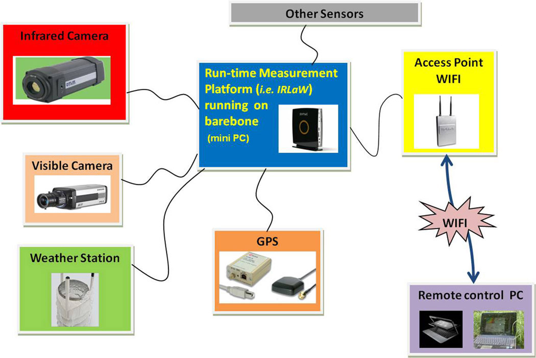

CLOUD FUNCTION ON e - COMMUNICATION
++++++++++++++++++++++++++++++++++++++++++++++++++++++++++++++++++++++++++++++++
Tidak ada komentar:
Posting Komentar