Hasil gambar untuk american flag electronic vibrations

Electronically Controlled Automatic Transmission (Automobile)

Electronically Controlled Automatic Transmission

An automatic transmission selects the most appropriate gear ratio for the prevailing engine speed, power train load and vehicle speed conditions, without any intervention by the driver. All gear shifting is carried out by the transmission system itself, and the driver only selects the desired operating mode with the selector lever. The Society of Automotive Engineers (SAE) has recommended that the selector should have the sequence PRND321in the case of a four-speed transmission as follows.
P (Park). In this position the transmission is in neutral and the transmission output shaft is locked by means of a parking pawl. The engine can be started.
R (Reverse). In this mode a single-speed reverse gear is selected and held. Engine braking is effective in this position, but the engine does not start.
N (Neutral). This mode is the same as Park, but the output shaft is not locked. The engine can be started.
D (Drive). This is the normal gear selection for forward motion. The vehicle may be operated from a standstill upto its maximum speed, with automatic upshifts and downshifts. The gearshift is made by the gearbox depending upon its assessment of vehicle speed and engine load. When rapid acceleration is required for overtaking, the driver can push the throttle pedal to its full travel to attain a speedy downshift into a lower gear. The engine does not start in D-drive range.
3 (Tliird). Operation of this gear varies between manufacturers. In general the transmission operates in D range, but is prevented from up shifting into fourth gear.
2 (Second). Operation of this gear also varies between manufacturers, but normally the transmission can only operate in first and second gear. Two is usually selected to provide engine braking when driving in hilly country or when towing.
1 (First). The transmission is locked in first gear to provide powerful engine braking. This is used when driving on steep hills or when towing.
To prevent inadvertent starting of the vehicle in a gear, a gearbox ‘inhibitor switch’ (also called a ‘neutral switch’) is positioned in series with the starter motor solenoid supply. The inhibitor switch contacts are closed when the selector lever is in Park or Neutral and so the engine can be started only in these positions. For additional safety the selector lever is equipped with a mechanical interlock, which does not allow the lever to be moved out of Park for example unless a spring-loaded release button is pressed.
The use of a microcomputer control system provides precise control of the hydraulic system thereby enhances the performance of the automatic transmission, offering. (i) Crisp and smooth gear shifts with consistent quality.
(ii) Perfectly timed gear shifts.
(Hi) Elimination of hunting shifts.
(iv) Protection of the transmission by constant monitoring of engine and transmission speed, temperature and so on.
(v) Driver-selectable shift pattern options for extra performance or economy, or for icy road conditions.
(ui) A simplified hydraulic control system.
An additional advantage of electronic control system is that the microcomputer can store diagnostic trouble codes. This greatly assists the mechanics in the quick repair of faulty transmission units.

Components and Parts of an Automatic Transmission

Figure 25.61 represents a sectional view of an electronically controlled automatic transmission used for front-wheel drive cars. Although transmission designs vary among manufacturers, the major components as described below are common to all.

Torque Converter.

The transmission bell housing is bolted to the rear of the engine block. This encloses the torque converter, which is secured to the engine flex-plate (a lightweight flywheel) by several small bolts. The torque converter is a virtually wear-free fluid coupling, which multiplies and transfers engine torque to the gear train through the input shaft.

Gear train.

The gear train is normally a compact compound epicyclic train capable of providing several different ratios. Commonly used gear trains include the Simpson, Ravigneaux and Wilson types. Variable-reluctance type sensors are installed in the transmission housing to monitor the input (turbine) and output shaft speeds.

Friction Elements.

Various hydraulically operated brake-bands, multi-plate clutches and multi-plate brakes are used to couple or lock the appropriate sets of planetary gear elements required for obtaining different gear ratios.

Oil Pump.

The hydraulic pressure required to operate the various friction elements (clutches and bands) is supplied by an oil pump, mounted just behind the torque converter, and driven by the engine through the torque converter housing. Oil pump output pressure (commonly known as line pressure) is regulated by an electronically controlled solenoid valve and directed to the appropriate clutches and bands by shift solenoids. The solenoid valve accurately modulates line pressure during gearshifts for smooth and rapid gear changes.

Electro-hydraulic Control Unit.

The electrohydraulic control unit, also known as the valve body, is generally positioned beneath the gear train and houses a number of mechanical and solenoid valves. These valves direct and modify the hydraulic fluid flow to the various clutches and brake-bands. The solenoid

Fig. 25.61. Electronically controlled automatic transmission for front-wheel drive vehicles.
valves execute gear change commands issued by the microcomputer in the transmission electronic control unit (transmission ECU). The transmission ECU thus controls the sequence and timing of gear ratio changes, and also the quality of the changes.

Transmission Housing.

The transmission housing is a lightweight aluminium casting and holds all of the transmission components as well as various sensors. It is usually designed for easy replacement of the valve and sensors with the transmission installed in the vehicle. At the base of the housing a sump pan is positioned and is kept filled with transmission oil, basically an SAE 20 grade mineral oil with various additives po improve its frictional and low-temperature properties. Various pressure taps are provided on the side of the housing to connect a pressure gauge during undertaking basic diagnostic tests.

Torque Converter Operation.

A torque converter transfers the crankshaft rotation to the automatic transmission. The converter absorbs the shocks of gear changing and dampens out vibrations, thereby permits the engine to smoothly drive the transmission from a standstill upto maximum speed. The torque converter has an external shape like a large metal donut, with a sealing weld around its outer edge. Internally, it has several elements mainly an impeller, a stator (sometimes called a reactor) and a turbine, as illustrated in Fig. 25.62.
The impeller is mounted to the torque converter shell and therefore is directly driven by the engine. The transmission pump is also driven by the engine, due to which with the engine running the torque converter is filled with transmission*fluid under pressure. As the impeller is rotated, centrifugal force throws fluid from the centre outwards so that fluid strikes the turbine blades causing the turbine to rotate, thereby turning the gearbox input shaft. Fluid leaving the turbine blades is then redirected by the specially curved stator blades back onto the impeller blades at such an angle that it helps the engine in driving the impeller (Fig. 25.63). It is this redirection of fluid energy that makes the torque converter to multiply engine torque by a factor upto two, providing good drive characteristics.
The torque converter “coupling point” occurs when the impeller, turbine and stator all revolve at about the same speed. The torque conversion ratio is 1:1, with a coupling efficiency of over 90%. During normal driving the torque conversion ratio continuously varies between about 2:1 and 1:1 depending upon the load on the engine.

Lockup Clutch Operation.

When a torque converter is operated in the coupling phase, a speed difference (slip) of upto 10% can exist between the impeller and the turbine. The slip causes a loss of fuel economy during high speed cruising, in addition to wasteful heating of the transmission oil. The torque converter lockup clutch was introduced in the 1970s in order to eliminate this slip.

Fig. 25.62. Torque converter construction.

Fig. 25.63. Exploded diagram of torque converter showing fluid path.
The operation of the lockup mechanism is illustrated Fig. 25.64. The lockup clutch uses a narrow friction lining 20-30 mm wide, bonded to a thin metal disc (sometimes called a piston), which is attached to turbine through a torsional damper spring. The transmission ECU controls fluid flow into the torque converter chamber with the help of solenoid valves. To lock-up the torque converter, the transmission ECU directs fluid into the port “C”, and allows exit via ports “D” and “E”. The lockup piston thus engages against the converter cover and the torque converter is placed in direct drive.
In order to disengage the lockup clutch, the transmission ECU actuates the solenoid valves to direct fluid into port “E” and allow it to exit from ports “C” and “D”. This causes the clutch piston to move away from the impeller so that the converter is placed in hydraulic drive enabling torque-multiplication.

Damper (Lock-up) Torque Converter.

The damper (or controlled slip) torque converter was introduced by Mitsubishi in 1982 and has since been used by several manufactures as a means of solving inherent drawbacks of conventional lockup torque converters. Damper torque converters cause partial lockup at low

Fig. 25.64. Torque converter lock up clutch. A. Engaged position. B. Disengaged position.
speeds in low gears, which is not possible with conventional lockup converters due to engagement shock and engine vibration.
In the damper torque converter the lockup clutch engagement is more accurately controlled by the transmission ECU by constantly monitoring the slip in the converter (i.e. the difference of the impeller input speed and the turbine output speed). The measured slip is then compared to a set point value stored in the transmission ECU’s memory. The ECU depending on the result of this comparison operates the lockup clutch fluid-control solenoid valve in a duty cycle mode at a high frequency (about 30 Hz) to vary the fluid flow to the converter providing just the right clutch contact pressure for the required slip. In this way clutch slip is controlled in the range 1-10% of input rpm, causing a smooth and vibration free operation.

Provision of Gear Ratios.

In a conventional automatic transmission an epicyclic gear train provides gear ratios. Figure 25.65 shows a Simpson gear-train capable of providing three forward gear ratios and reverse. The selection of the appropriate ratio depends on the application of hydraulic pressure to clutches and brake-bands operating in a set pattern. The electro-hydraulic control valves regulate the engagement of friction element based on the signals received from the transmission ECU and direct line pressure accordingly.

Fig. 25.65. Simpson gear-train.
Low gear is obtained by engaging the forward clutch, so that engine power is applied to the ring-gear of the first gear-set, thus rotating the planet wheels clockwise to drive the common sun gear anticlockwise. The one-way sprag clutch prevents rotation of the planet carrier of the second gear-set and therefore the planet wheels rotate to drive the output shaft in compound reduction. Engine braking is accomplished by applying the low reverse brake band to disable the free wheeling effect of the sprag clutch.
To select intermediate gear, the intermediate brake-band is applied to lock the common sun gear against rotation. With the forward clutch engaged, power flows to the first ring-gear, thereby driving the planet wheels around the sun gear and rotating the output shaft in simple reduction drive.
To obtain high gear, both the forward and the reverse-high clutches are engaged, so that the sun gear locks to the first ring-gear. The whole gear-train revolves at the same speed as the input shaft giving direct drive.
Reverse gear is obtained by engaging the reverse-high clutch and the low-reverse brakeband so that drive is transmitted through the sub-gear to the planet wheels of the second gear-set, as a result the ring-gear turns in the opposite direction to the input shaft. The low reverse brake band holds the planet carrier of the second gear set against rotation, causing the output shaft to turn,
25.27.2.

Transmission Control System

The operation of a typical electronically controlled transmission system is illustrated on Fig. 25.66, which has been installed by a number of vehicle manufacturers, including Mazda, Nissan and Rover. The system offers four forward gears, controlled by a transmission ECU, which communicates with the engine ECU to provide total power train management. The transmission ECU takes decisions based on electrical signals received from various sensors located on the engine and gearbox. ECU’s microcomputer stores data relating to the ideal gear for every speed and load condition, along with correction factors for engine and transmission temperatures, brake pedal depression and so on. Using this corrected data the transmission ECU energizes solenoid valves to engage the most suitable gear ratio for the existing driving conditions. The transmission ECU also provides a self-diagnosis function on some of the sensors and operates a fail-safe mode if a fault is found. This electronically controlled automatic transmission offers some typical features as follows.

Fig. 25.66. Transmission control system structure (Mazda).
(i) It incorporates a duty-cycle solenoid valve to vary line pressure so that clutch and brake-band engagement force is optimized during each gearshift.
(«’) It controls the engine and transmission totally by reducing the engine torque during
gearshifts, thereby producing smooth gear change. (Hi) It contains a duty cycle lockup solenoid, which causes controlled-slip lockup at low speeds and provides less shock when engaging full lockup at cruising speeds.
(iv) It includes optional control programs, selected by the driver, allowing POWER or HOLD shift patterns to be engaged. The POWER program delays each upshift by a few hundred rpm to permit a sporty driving style. HOLD causes the transmission ECU to hold a selected gear, which is useful when driving in hilly country or on difficult road surfaces.
25.27.3.

The Transmission ECU Input System

The heart of the transmission control system is the transmission ECU, which accepts inputs from various sensors and communicates with the engine ECU.
The pulse generator is a magnetic pickup, located in the upper part of the transaxle casing and detects the gear-train’s reverse-forward drum speed, i.e. the torque converter output speed.
The speedometer sensor is a magnetic pickup sensor, which detects the gearbox’s output shaft speed, i.e. the vehicle speed.
The throttle sensor and idle switch is a combination sensor containing a potentiometer and also a pair of contacts, which close when the engine is at idle. It detects throttle angle and hence engine load. When idle is detected, and the vehicle is stationary, the transmission ECU engages second gear. This minimizes torque loads on the transaxle and reduces creep when stationary in traffic. First gear is engaged as soon as the ECU detects movement of the accelerator pedal.
The inhibitor switch reports the position of the selector lever to the transmission ECU. It also prevents operation of the starter motor if it is not in either Park or Neutral.
The HOLD switch is a press-button switch located on the selector lever. It is used by the driver to instruct the ECU to hold a particular gear ratio, for example when descending a hill. When HOLD is in use the HOLD indicator glows up.
The stoplight switch detects when the brakes have been used. If the brakes are applied while the torque converter is in lockup, the transmission ECU releases lockup to provide a smooth deceleration.
The O/D inhibit signal is used together with the cruise control. It prevents the transmission from shifting into overdrive (fourth gear) when the cruise control is operational and vehicle speed is more than 8 kmph below the set cruising speed.
The ATF thermosensor is a thermistor, which registers the temperature of the transmission fluid. The ECU utilises this information to modify line pressure at extremes of temperature, so that the fluid’s higher viscosity at low temperatures and the danger of overheating at high temperature are taken into account.
An engine rpm signal is taken from the ignition coil primary winding.
An atmospheric pressure sensor sends a signals to the transmission ECU when the measured atmospheric pressure indicates that the vehicle is at a height of 1500 m or more. The engine develops less power at high altitudes and, therefore, the ECU modifies the gearshift points accordingly.
25.27.4.

The Transmission ECU Output System

To change a gear, the transmission ECU sends signals to seven solenoid valves located in the valve body of the transmission. The solenoid valves are either of the ON/OFF type or the duty-cycle type where a variable pressure is required. The three shift solenoids (1-2, 2-3, 3-4 shift) are either ON or OFF and direct line pressure to the shift valves. The transmission ECU selects a programmed shift pattern based on selector position and then receives signals for vehicle speed and throttle opening angle. Based on the results of calculations performed on these signal values, the ECU sets the gear ratio and energizes the appropriate solenoid valve (Fig. 25.67).
The 3-2 timing solenoid directs pressure to the 3-2 timing valve and controls the precise timing of clutch and brake-band engagement.
The lockup control solenoid directs line pressure to the torque converter lockup system when the transmission ECU energizes it at appropriate time. This solenoid is either ON or OFF
type.
The lockup pressure reducing solenoid controls engagement slip in the lockup clutch. This solenoid is operated on a duty cycle basis (at about 30 Hz) and modifies the engagement force on the clutch piston. The duty cycle is continuously modified to maintain the target slip value.

Fig. 25.67. Solenoid operation and gear selection (Mazda).
The engagement force, applied to the brake-band and multi-plate clutches, is controlled by the pressure solenoid. This is a 30 Hz duty cycle control valve, which modifies the line pressure depending on the signals receives from the ECU. Line pressure is increased in proportion to throttle opening angle, causing increased clamping force on the friction members to cope with greater engine torque. During gearshifts the line pressure is momentarily reduced to minimize shift shock.
25.27.5.

Total Engine and Transmission Control

One of the key features of most modern automatic transmission is shift comfort, especially those with four or five gears where shift frequency is likely to be greater than in three speed arrangements. To reduce shift shock the transmission and engine ECUs exchange digital data so that the engine output torque during gear-shifting is temporarily lowered. This feature of the control system is known as total controlor engine intervention. Total control reduces torque fluctuations at the transmission output shaft and offers several additional advantages as follows.
(i) A lower line pressure can be used to clamp the friction elements, so that engagement shock is reduced.
(H) Reduced slippage of the friction elements during engagement causes less lining wear. As a result less heating of the transmission fluid takes place, thereby extending its life and increasing the transmission efficiency.
(Hi) Less slippage of the friction elements occurs.
To achieve engine intervention, either fuel injection is cut off or the ignition timing is retarded (or a combination of both). In the Mazda GF4A-EL transaxle, fuel injection is cut off during up shifting and the ignition timing is retarded during downshift (Fig. 25.68).

Fig. 25.68. Engine torque reduction during gear-changing (Mazda).

Fuel Injection Cut Off Control.

When the transmission ECU decides for an up-shift (1-2 or 2-3 shift), it sends a “Reduce Torque Signal 1″ (logic 1) to the engine ECU. If a fuel cut takes place considering the engine conditions, the engine ECU confirms its action by sending a “Torque Reduced Signal” back to the transmission ECU. The transmission ECU then performs the gearshift and removes the Reduce Torque Signal 1 to reinstate fuel injection.

Ignition Timing Retardation Control.

When the transmission ECU judges the requirement of a downshift (3-2 or 2-1 shift), it sends a “Reduce Torque Signal 2″ (logic 2) to the engine ECU. The engine ECU then reduces the spark timing by several degrees to lower the engine torque and sends a “Torque Reduced Signal” to transmission ECU as confirmation. Once the down-shift is completed by the transmission ECU, the Reduce Torque Signal 2 is removed and the ignition timing is restored to normal.
25.27.6.

Feedback Control

Another method of providing smoother gear changes is through feedback control of the friction element engagement force. This can be achieved either by directly monitoring various fluid pressures using sensors in the transmission, which is incorporated on some Chrysler
transmissions or by monitoring the instantaneous slippage in the transmission (Fig. 25.69) using speed sensor signals.

Fig. 25.69. Feedback control of clutch engagement pressure (Mitsubishi).
The latter technique depends on accurate control of the line pressure during gear engagement. This ensures variations in the input shaft speed, and hence the variations in band/clutch slip within a specified range. As a result smooth and consistent shift quality, irrespective of friction material condition and fluid temperature, is achieved.
The speed of the gearbox input shaft, during gear changes, is measured and compared against that of the output shaft. The transmission ECU then calculates the speed gradient of the input shaft {i.e. its declaration). Whenever this calculated valve becomes more or less than a preprogrammed value the drive duty to the line pressure solenoid is lowered or raised accordingly to restore it for ensuring a smooth and steady engagement.

Dynamics and Vibrations
Conservation laws for systems of particles

the following general concepts:

The linear impulse of a force
The angular impulse of a force
The power transmitted by a force
The work done by a force
The potential energy of a force.
The linear momentum of a particle (or system of particles)
The angular momentum of a particle, or system of particles.
The kinetic energy of a particle, or system of particles
The linear impulse momentum relations for a particle, and conservation of linear momentum
The principle of conservation of angular momentum for a particle
The principle of conservation of energy for a particle or system of particles.

We will also illustrate how these concepts can be used in engineering calculations. As you will see, to applying these principles to engineering calculations you will need two things: (i) a thorough understanding of the principles themselves; and (ii) Physical insight into how engineering systems behave, so you can see how to apply the theory to practice. The first is easy. The second is hard, and people who can do this best make the best engineers.

Work, Power, Potential Energy and Kinetic Energy relations

The concepts of work, power and energy are among the most powerful ideas in the physical sciences. Their most important application is in the field of thermodynamics, which describes the exchange of energy between interacting systems. In addition, concepts of energy carry over to relativistic systems and quantum mechanics, where the classical versions of Newton’s laws themselves no longer apply.

In this section, we develop the basic definitions of mechanical work and energy, and show how they can be used to analyze motion of dynamical systems. Future courses will expand on these concepts further.

Definition of the power and work done by a force

Suppose that a force F acts on a particle that moves with speed v.

By definition:

The Power developed by the force, (or the rate of work done by the force) is

. If both force and velocity are expressed in Cartesian components, then

Work has units of Nm/s, or `Watts’ in SI units.

The work done by the force during a time interval

The work done by the force can also be calculated by integrating the force vector along the path traveled by the force, as

where

are the initial and final positions of the force.

Work has units of Nm in SI units, or `Joules’

A moving force can do work on a particle, or on any moving object. For example, if a force acts to stretch a spring, it is said to do work on the spring.

Definition of the power and work done by a concentrated moment, couple or torque.

‘Concentrated moment, ‘Couple’ and `Torque’ are different names for a ‘generalized force’ that causes rotational motion without causing translational motion. These concepts are not often used to analyze motion of particles, where rotational motion is ignored

the only application might be to analyze rotational motion of a massless frame connected to one or more particles. For completeness, however, the power-work relations for moments are listed in this section and applied to some simple problems. To do this, we need briefly to discuss how rotational motion is described.

Definition of an angular velocity vector Visualize a spinning object, like the cube shown in the figure. The box rotates about an axis

in the example, the axis is the line connecting two cube diagonals. In addition, the object turns through some number of revolutions every minute. We would specify the angular velocity of the shaft as a vector

, with the following properties:

The direction of the vector is parallel to the axis of the shaft (the axis of rotation). This direction would be specified by a unit vector n parallel to the shaft
There are, of course, two possible directions for n. By convention, we always choose a direction such that, when viewed in a direction parallel to n (so the vector points away from you) the shaft appears to rotate clockwise. Or conversely, if n points towards you, the shaft appears to rotate counterclockwise. (This is the `right hand screw convention’)


Viewed along n	Viewed in direction opposite to n

The magnitude of the vector is the angular speed of the object, in radians per second. If you know the revs per minute n turned by the shaft, the number of radians per sec follows as . The magnitude of the angular velocity is often denoted by

The angular velocity vector is then

Since angular velocity is a vector, it has components

in a fixed Cartesian basis.

Rate of work done by a torque or moment: If a moment

acts on an object that rotates with angular velocity

, the rate of work done on the object by M is

Simple examples of power and work calculations

Example 1: An aircraft with mass 45000 kg flying at 200 knots (102m/s) climbs at 1000ft/min. Calculate the rate of work done on the aircraft by gravity.

The gravitational force is

, and the velocity vector of the aircraft is

. The rate of work done on the aircraft is therefore

Substituting numbers gives

Example 2: Calculate a formula for the work required to stretch a spring with stiffness kand unstretched length

from length

to length

The figure shows a spring that held fixed at A and is stretched in the horizontal direction by a force

acting at B. At some instant the spring has length

. The spring force law states that the force acting on the spring at B is related to the length of the spring x by

The position vector of the force is

, and therefore the work done is

Example 3: Calculate the work done by gravity on a satellite that is launched from the surface of the earth to an altitude of 250km (a typical low earth orbit).

Assumptions

The earth’s radius is 6378.145km
The mass of a typical satellite is 4135kg - see , e.g. http://www.astronautix.com/craft/hs601.htm
The Gravitational parameter (G= gravitational constant; M=mass of earth)
We will assume that the satellite is launched along a straight line path parallel to the i direction, starting the earths surface and extending to the altitude of the orbit. It turns out that the work done is independent of the path, but this is not obvious without more elaborate and sophisticated calculations.

Calculation:

The gravitational force on the satellite is

The work done follows as

Substituting numbers gives J (be careful with units if you work with kilometers the work done is in N-km instead of SI units Nm)

Example 4: A Ferrari Testarossa skids to a stop over a distance of 250ft. Calculate the total work done on the car by the friction forces acting on its wheels.

Assumptions:

A Ferrari Testarossa has mass 1506kg (see http://www.ultimatecarpage.com/car/1889/Ferrari-Testarossa.html)
The coefficient of friction between wheels and road is of order 0.8
We assume the brakes are locked so all wheels skid, and air resistance is neglected

Calculation The figure shows a free body diagram. The equation of motion for the car is

The vertical component of the equation of motion yields
The friction law shows that
The position vectors of the car’s front and rear wheels are . The work done follows as. We suppose that the rear wheel starts at some point when the brakes are applied and skids a total distance d.

The work done follows as . Substituting numbers gives .

Example 5: The figure shows a box that is pushed up a slope by a force P. The box moves with speed v. Find a formula for the rate of work done by each of the forces acting on the box.

The figure shows a free body diagram. The force vectors are

1. Applied force

2. Friction

3. Normal reaction

4. Weight

The velocity vector is

Evaluating the dot products

for each formula, and recalling that

gives

1. Applied force

2. Friction

3. Normal reaction

4. Weight

Force N	Draw (cm)
0	0
40	10
90	20
140	30
180	40
220	50
270	60

Example 6: The table lists the experimentally measured force-v-draw data for a long-bow. Calculate the total work done to draw the bow.

In this case we don’t have a function that specifies the force as a function of position; instead, we have a table of numerical values. We have to approximate the integral

numerically. To understand how to do this, remember that integrating a function can be visualized as computing the area under a curve of the function, as illustrated in the figure.

We can estimate the integral by dividing the area into a series of trapezoids, as shown. Recall that the area of a trapezoid is (base x average height), so the total area of the function is

You could easily do this calculation by hand

but for lazy people like me MATLAB has a convenient function called `trapz’ that does this calculation automatically. Here’s how to use it

>> draw = [0,10,20,30,40,50,60]*0.01;

>> force = [0,40,90,140,180,220,270];

>> trapz(draw,force)

ans =

80.5000

So the solution is 80.5J

Definition of the potential energy of a conservative force

Preamble: Textbooks nearly always define the `potential energy of a force.’ Strictly speaking, we cannot define a potential energy of a single force

instead, we need to define the potential energy of a pair of forces. A force can’t exist by itself

there must always be an equal and opposite reaction force acting on a second body. In all of the discussion to be presented in this section, we implicitly assume that the reaction force is acting on a second body, which is fixed at the origin. This simplifies calculations, and makes the discussion presented here look like those given in textbooks, but you should remember that the potential energy of a force pair is always a function of the relative positions of the two forces.

With that proviso, consider a force F acting on a particle at some position r in space. Recall that the work done by a force that moves from position vector

to position vector

In general, the work done by the force depends on the path between

. For some special forces, however, the work done is independent of the path. Such forces are said to be conservative.

For a force to be conservative:

The force must be a function only of its position

i.e. it can’t depend on the velocity of the force, for example.

The force vector must satisfy

Examples of conservative forces include gravity, electrostatic forces, and the forces exerted by a spring. Examples of non-conservative (or should that be liberal?) forces include friction, air resistance, and aerodynamic lift forces.

The potential energy of a conservative force is defined as the negative of the work done by the force in moving from some arbitrary initial position

to a new position

, i.e.

The constant is arbitrary, and the negative sign is introduced by convention (it makes sure that systems try to minimize their potential energy). If there is a point where the force is zero, it is usual to put

at this point, and take the constant to be zero.

Note that

The potential energy is a scalar valued function
The potential energy is a function only of the position of the force. If we choose to describe position in terms of Cartesian components , then .
The relationship between potential energy and force can also be expressed in differential form (which is often more useful for actual calculations) as

If we choose to work with Cartesian components, then

Occasionally, you might have to calculate a potential energy function by integrating forces

for example, if you are interested in running a molecular dynamic simulation of a collection of atoms in a material, you will need to describe the interatomic forces in some convenient way. The interatomic forces can be estimated by doing quantum-mechanical calculations, and the results can be approximated by a suitable potential energy function. Here are a few examples showing how you can integrate forces to calculate potential energy

Example 1: Potential energy of forces exerted by a spring. A free body diagram showing the forces exerted by a spring connecting two objects is shown in the figure.

The force exerted by a spring is

The position vector of the force is
The potential energy follows as

where we have taken the constant to be zero.

Example 2: Potential energy of electrostatic forces exerted by charged particles.

The figure shows two charged particles a distance x apart. To calculate the potential energy of the force acting on particle 2, we place particle 1 at the origin, and note that the force acting on particle 2 is

where

and

are the charges on the two particles, and

is a fundamental physical constant known as the Permittivity of the medium surrounding the particles. Since the force is zero when the particles are infinitely far apart, we take

at infinity. The potential energy follows as

Table of potential energy relations

In practice, however, we rarely need to do the integrals to calculate the potential energy of a force, because there are very few different kinds of force. For most engineering calculations the potential energy formulas listed in the table below are sufficient.

Type of force	Force vector	Potential energy
Gravity acting on a particle near earths surface
Gravitational force exerted on mass m by mass Mat the origin
Force exerted by a spring with stiffness k and unstretched length
Force acting between two charged particles
Force exerted by one molecule of a noble gas (e.g. He, Ar, etc) on another (Lennard Jones potential). a is the equilibrium spacing between molecules, and E is the energy of the bond.

Potential energy of concentrated moments exerted by a torsional spring

A potential energy cannot usually be defined for concentrated moments, because rotational motion is itself path dependent (the orientation of an object that is given two successive rotations depends on the order in which the rotations are applied). A potential energy can, however, be defined for the moments exerted by a torsional spring.

A solid rod is a good example of a torsional spring. You could take hold of the ends of the rod and twist them, causing one end to rotate relative to the other. To do this, you would apply a moment or a couple to each end of the rod, with direction parallel to the axis of the rod. The angle of twist increases with the moment. Various torsion spring designs used in practice are shown in the picture

the image is from

http://www.mollificio.lombardo.molle.com/springs/torsion_springs.html

More generally, a torsional spring resists rotation, by exerting equal and opposite moments on objects connected to its ends. For a linear spring the moment is proportional to the angle of rotation applied to the spring.

The figure shows a formal free body diagram for two objects connected by a torsional spring. If object A is held fixed, and object B is rotated through an angle

about an axis parallel to a unit vector n, then the spring exerts a moment

on object B where

is the torsional stiffness of the spring. Torsional stiffness has units of Nm/radian.

The potential energy of the moments exerted by the spring can be determined by computing the work done to twist the spring through an angle

The work done by a moment M due to twisting through a very small angle about an axis parallel to a vector n is

The potential energy is the negative of the total work done by M, i.e.

Definition of the Kinetic Energy of a particle

Consider a particle with mass m which moves with velocity

. By definition, its kinetic energy is

Power-Work-kinetic energy relations for a single particle

Consider a particle with mass m that moves under the action of a force F. Suppose that

At some time the particle has some initial position , velocity and kinetic energy
At some later time the particle has a new position r, velocity and kinetic energy .
Let denote the rate of work done by the force
Let be the total work done by the force

The Power-kinetic energy relation for the particle states that the rate of work done by F is equal to the rate of change of kinetic energy of the particle, i.e.

This is just another way of writing Newton’s law for the particle: to see this, note that we can take the dot product of both sides of F=ma with the particle velocity

To see the last step, do the derivative using the Chain rule and note that

The Work-kinetic energy relation for a particle says that the total work done by the force F on the particle is equal to the change in the kinetic energy of the particle.

This follows by integrating the power-kinetic energy relation with respect to time.

Examples of simple calculations using work-power-kinetic energy relations

There are two main applications of the work-power-kinetic energy relations. You can use them to calculate the distance over which a force must act in order to produce a given change in velocity. You can also use them to estimate the energy required to make a particle move in a particular way, or the amount of energy that can be extracted from a collection of moving particles (e.g. using a wind turbine)

Example 1: Estimate the minimum distance required for a 14 wheeler that travels at the RI speed-limit to brake to a standstill. Is the distance to stop any different for a Toyota Echo?

This problem can be solved by noting that, since we know the initial and final speed of the vehicle, we can calculate the change in kinetic energy as the vehicle stops. The change in kinetic energy must equal the work done by the forces acting on the vehicle

which depends on the distance slid. Here are the details of the calculation.

Assumptions:

We assume that all the wheels are locked and skid over the ground (this will stop the vehicle in the shortest possible distance)
The contacts are assumed to have friction coefficient
The vehicle is idealized as a particle.
Air resistance will be neglected.

Calculation:

The figure shows a free body diagram.
The equation of motion for the vehicle is

The vertical component of the equation shows that

The friction force follows as
If the vehicle skids for a distance d, the total work done by the forces acting on the vehicle is

The work-energy relation states that the total work done on the particle is equal to its change in kinetic energy. When the brakes are applied the vehicle is traveling at the speed limit, with speed V; at the end of the skid its speed is zero. The change in kinetic energy is therefore . The work-energy relation shows that

Substituting numbers gives

This simple calculation suggests that the braking distance for a vehicle depends only on its speed and the friction coefficient between wheels and tires. This is unlikely to vary much from one vehicle to another. In practice there may be more variation between vehicles than this estimate suggests, partly because factors like air resistance and aerodynamic lift forces will influence the results, and also because vehicles usually don’t skid during an emergency stop (if they do, the driver loses control)

the nature of the braking system therefore also may change the prediction.

Example 3: Compare the power consumption of a Ford Excursion to that of a Chevy Cobalt during stop-start driving in a traffic jam.

During stop-start driving, the vehicle must be repeatedly accelerated to some (low) velocity; and then braked to a stop. Power is expended to accelerate the vehicle; this power is dissipated as heat in the brakes during braking. To calculate the energy consumption, we must estimate the energy required to accelerate the vehicle to its maximum speed, and estimate the frequency of this event.

Calculation/Assumptions:

We assume that the speed in a traffic jam is low enough that air resistance can be neglected.
The energy to accelerate to speed V is .
We assume that the vehicle accelerates and brakes with constant acceleration if so, its average speed is V/2.
If the vehicle travels a distance d between stops, the time between two stops is 2d/V.
The average power is therefore .
Taking V=15mph (7m/s) and d=200ft (61m) are reasonable values the power is therefore 0.03m, with m in kg. A Ford Excursion weighs 9200 lb (4170 kg), requiring 125 Watts (about that of a light bulb) to keep moving. A Chevy Cobalt weighs 2681lb (1216kg) and requires only 36 Watts a very substantial energy saving.

Reducing vehicle weight is the most effective way of improving fuel efficiency during slow driving, and also reduces manufacturing costs and material requirements. Another, more costly, approach is to use a system that can recover the energy during braking

this is the main reason that hybrid vehicles like the Prius have better fuel economy than conventional vehicles.

Example 4: Estimate the power that can be generated by a wind turbine.

The figure shows a wind turbine. The turbine blades deflect the air flowing past them: this changes the air speed and so exerts a force on the blades. If the blades move, the force exerted by the air on the blades does work

this work is the power generated by the turbine. The rate of work done by the air on the blades must equal the change in kinetic energy of the air as it flows past the blades. Consequently, we can estimate the power generated by the turbine by calculating the change in kinetic energy of the air flowing through it.

To do this properly needs a very sophisticated analysis of the air flow around the turbine. However, we can get a rather crude estimate of the power by assuming that the turbine is able to extract all the energy from the air that flows through the circular area swept by the blades.

Calculation: Let V denote the wind speed, and let

denote the density of the air.

1. In a time t, a cylindrical region of air with radius R and height Vt passes through the fan.

2. The cylindrical region has mass

3. The kinetic energy of the cylindrical region of air is

4. The rate of flow of kinetic energy through the fan is therefore

5. If all this energy could be used to do work on the fan blades the power generated would be

Representative numbers are (i) Air density 1.2

; (ii) air speed 25mph (11 m/sec); (iii) Radius 30m

This gives 1.8MW. For comparison, a nuclear power plant generates about 500-1000 MW.

A more sophisticated calculation (which will be covered in EN810) shows that in practice the maximum possible amount of energy that can be extracted from the air is about 60% of this estimate. On average, a typical household uses about a kW of energy; so a single turbine could provide enough power for about 5-10 houses.

Energy relations for a conservative system of particles.

The figure shows a `system of particles’

this is just a collection of objects that we might be interested in, which can be idealized as particles. Each particle in the system can experience forces applied by:

Other particles in the system (e.g. due to gravity, electric charges on the particles, or because the particles are physically connected through springs, or because the particles collide). We call these internal forces acting in the system. We will denote the internal force exerted by the ith particle on the jth particle by

. Note that, because every action has an equal and opposite reaction, the force exerted on the jth particle by the ith particle must be equal and opposite, to

, i.e.

Forces exerted on the particles by the outside world (e.g. by externally applied gravitational or electromagnetic fields, or because the particles are connected to the outside world through mechanical linkages or springs). We call these external forces acting on the system, and we will denote the external force on the i th particle by

We define the total external work done on the system during a time interval

as the sum of the work done by the external forces.

The total work done can also include a contribution from external moments acting on the system.

The system of particles is conservative if all the internal forces in the system are conservative. This means that the particles must interact through conservative forces such as gravity, springs, electrostatic forces, and so on. The particles can also be connected by rigid links, or touch one another, but contacts between particles must be frictionless.

If this is the case, we can define the total potential energy of the system as the sum of potential energies of all the internal forces.

We also define the total kinetic energy

of the system as the sum of kinetic energies of all the particles.

The work-energy relation for the system of particles can then be stated as follows. Suppose that

At some time the system has and kinetic energy
At some later time the system has kinetic energy .
Let denote the potential energy of the force at time
Let denote the potential energy of the force at time
Let denote the total work done on the system between

Work Energy Relation: This law states that the external work done on the system is equal to the change in total kinetic and potential energy of the system.

We won’t attempt to prove this result - the proof is conceptually very straightforward: it simply involves summing the work-energy relation for all the particles in the system; and we’ve already seen that the work-energy relations are simply a different way of writing Newton’s laws. But when written out the sums make the proof look scary and difficult to follow so we’ll spare you the gory details. If you are interested, ask us (or better still see if you can do it for yourself!)

Energy conservation law For the special case where no external forces act on the system, the total energy of the system is constant

It is worth making one final remark before we turn to applications of these law. We often invoke the principle of conservation of energy when analyzing the motion of an object that is subjected to the earth’s gravitational field. For example, the first problem we solve in the next section involves the motion of a projectile launched from the earth’s surface. We usually glibly say that `the sum of the potential and kinetic energies of the particle are constant’

and if you’ve done physics courses you’ve probably used this kind of thinking. It is not really correct, although it leads to a more or less correct solution.

Properly, we should consider the earth and the projectile together as a conservative system. This means we must include the kinetic energy of the earth in the calculation, which changes by a small, but finite, amount due to gravitational interaction with the projectile. Fortunately, the principle of conservation of linear momentum (to be covered later) can be used to show that the change in kinetic energy of the earth is negligibly small compared to that of the particle.

Examples of calculations using kinetic and potential energy in conservative systems

The kinetic-potential energy relations can be used to quickly calculate relationships between the velocity and position of an object. Several examples are provided below.

Example 1: (Boring FE exam question) A projectile with mass m is launched from the ground with velocity

at angle

. Calculate an expression for the maximum height reached by the projectile.

If air resistance can be neglected, we can regard the earth and the projectile together as a conservative system. We neglect the change in the earth’s kinetic energy. In addition, since the gravitational force acting on the particle is vertical, the particle’s horizontal component of velocity must be constant.

Calculation:

Just after launch, the velocity of the particle is
The kinetic energy of the particle just after launch is . Its potential energy is zero.
At the peak of the trajectory the vertical velocity is zero. Since the horizontal velocity remains constant, the velocity vector at the peak of the trajectory is . The kinetic energy at this point is therefore
Energy is conserved, so

Example 2: You are asked to design the packaging for a sensitive instrument. The packaging will be made from an elastic foam, which behaves like a spring. The specifications restrict the maximum acceleration of the instrument to 15g. Estimate the thickness of the packaging that you must use.

This problem can be solved by noting that (i) the max acceleration occurs when the packaging (spring) is fully compressed and so exerts the maximum force on the instrument; (ii) The velocity of the instrument must be zero at this instant, (because the height is a minimum, and the velocity is the derivative of the height); and (iii) The system is conservative, and has zero kinetic energy when the package is dropped, and zero kinetic energy when the spring is fully compressed.

Assumptions:

The package is dropped from a height of 1.5m
The effects of air resistance during the fall are neglected
The foam is idealized as a linear spring, which can be fully compressed.

Calculations: Let h denote the drop height; let d denote the foam thickness.

The potential energy of the system just before the package is dropped is mgh
The potential energy of the system at the instant when the foam is compressed to its maximum extent is
The total energy of the system is constant, so

The figure shows a free body diagram for the instrument at the instant of maximum foam compression. The resultant force acting on the instrument is , so its acceleration follows as . The acceleration must not exceed 15g, so

Dividing (3) by (4) shows that

The thickness of the protective foam must therefore exceed 18.8cm.

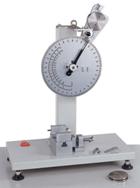
Example 3: The Charpy Impact Test is a way to measure the work of fracture of a material (i.e. the work per unit area required to separate a material into two pieces).

It consists of a pendulum, which swings down from a prescribed initial angle to strike a specimen. The pendulum fractures the specimen, and then continues to swing to a new, smaller angle on the other side of the vertical. The scale on the pendulum allows the initial and final angles to be measured. The goal of this example is to deduce a relationship between the angles and the work of fracture of the specimen.

The figure shows the pendulum before and after it hits the specimen.

The potential energy of the mass before it is released is . Its kinetic energy is zero.
The potential energy of the mass when it comes to rest after striking the specimen is . The kinetic energy is again zero.

The work of fracture is equal to the change in potential energy -

Example 4: Estimate the maximum distance that a long-bow can fire an arrow.

We can do this calculation by idealizing the bow as a spring, and estimating the maximum force that a person could apply to draw the bow. The energy stored in the bow can then be estimated, and energy conservation can be used to estimate the resulting velocity of the arrow.

Assumptions

The long-bow will be idealized as a linear spring
The maximum draw force is likely to be around 60lbf (270N)
The draw length is about 2ft (0.6m)
Arrows come with various masses typical range is between 250-600 grains (16-38 grams)
We will neglect the mass of the bow (this is not a very realistic assumption)

Calculation: The calculation needs two steps: (i) we start by calculating the velocity of the arrow just after it is fired. This will be done using the energy conservation law; and (ii) we then calculate the distance traveled by the arrow using the projectile trajectory equations derived in the preceding chapter.

Just before the arrow is released, the spring is stretched to its maximum length, and the arrow is stationary. The total energy of the system is , where L is the draw length and k is the stiffness of the bow.
We can estimate values for the spring stiffness using the draw force: we have that , so . Thus .
Just after the arrow is fired, the spring returns to its un-stretched length, and the arrow has velocity V. The total energy of the system is , where m is the mass of the arrow
The system is conservative, therefore
We suppose that the arrow is launched from the origin at an angle to the horizontal. The horizontal and vertical components of velocity are . The position vector of the arrow can be calculated using the method outlined in Section 3.2.2 the result is

We can calculate the distance traveled by noting that its position vector when it lands is di. This gives

where t is the time of flight. The i and j components of this equation can be solved for t and d, with the result

The arrow travels furthest when fired at an angle that maximizes

- i.e. 45 degrees. The distance follows as

Substituting numbers gives 2064m for a 250 grain arrow over a mile! Of course air resistance will reduce this value, and in practice the kinetic energy associated with the motion of the bow and bowstring (neglected here) will reduce the distance.

Example 5: Find a formula for the escape velocity of a space vehicle as a function of altitude above the earths surface.

The term ‘Escape velocity’ means that the space vehicle has a large enough velocity to completely escape the earth’s gravitational field

i.e. the space vehicle will never stop after being launched.

Assumptions

The space vehicle is initially in orbit at an altitude h above the earth’s surface
The earth’s radius is 6378.145km
While in orbit, a rocket is burned on the vehicle to increase its speed to v (the escape velocity), placing it on a hyperbolic trajectory that will eventually escape the earth’s gravitational field.
The Gravitational parameter (G= gravitational constant; M=mass of earth)

Calculation

Just after the rocket is burned, the potential energy of the system is , while its kinetic energy is
When it escapes the earth’s gravitational field (at an infinite height above the earth’s surface) the potential energy is zero. At the critical escape velocity, the velocity of the spacecraft at this point drops to zero. The total energy at escape is therefore zero.
This is a conservative system, so

A typical low earth orbit has altitude of 250km. For this altitude the escape velocity is 10.9km/sec.

4.1.11 Force, Torque and Power curves for actuators and motors

Concepts of power and work are particularly useful to calculate the behavior of a system that is driven by a motor. Calculations like this are described in more detail in Section 4.12. In this section, we discuss the relationships between force, torque, speed and power for motors.

There are many different types of motor, and each type has its own unique characteristics. They all have the following features in common, however:

The motors convert some non-mechanical form of energy into mechanical work. For example, an electric motor converts electrical energy; an internal combustion engine, your muscles, and other molecular motors convert chemical energy, and so on.

A linear motor or linear actuator applies a force to an object (or more accurately, it applies roughly equal and opposite forces on two objects connected to its ends). Your muscles are good examples of linear actuators. You can buy electrical or hydraulically powered actuators as well.

The forces applied by an actuator depend on (i) the amount of power supplied to the actuator electrical, chemical, etc; and (ii) the rate of contraction, or stretching, of the actuator. The typical variation of force with stretch rate is shown in the figure. The figure assumes that the actuator pulls on the objects attached to its ends (like a muscle); but some actuators will push rather than pull; and some can do both. If the actuator extends slowly and is not rotating it behaves like a two-force member, and the forces exerted by its two ends are equal and opposite.

A rotary motor or rotary actuator applies a moment or torque to an object (or, again, more precisely it applies equal and opposite moments to two objects). Electric motors, internal combustion engines, bacterial motors are good examples of rotary motors.

The torques exerted by a rotary actuator depend on (i) the amount of power supplied to the actuator electrical, chemical, etc; and (ii) the relative velocity of the two objects on which the forces act. The typical variation of force with external power applied and with relative velocity is shown in the figure. An electric motor applies a large torque when it is stationary, and its torque decreases with rotational speed. An internal combustion engine applies no torque when it is stationary. It’s torque is greatest at some intermediate speed, and decreases at high speed.

The power curve describes the variation of the rate of work done by an actuator or motor with its extension or contraction rate or rotational speed. Note that

The rate of work done (or power expended) by a linear actuator that applies forces , to the objects attached to its two ends can be calculated as , where and are the velocities of the two ends.
The rate of work (or power expended) by a rotational motor that applies moments , to the objects attached to its two ends is .

Typical power curves for motors and actuators are sketched in the figures.

The efficiency of a motor or actuator is the ratio of the rate of work done by the forces or moments exerted by the motor to the electrical or chemical power. The efficiency is always less than 1 because some fraction of the power supplied to the motor is dissipated as heat. An electric motor has a high efficiency; heat engines such as an internal combustion engine have a much lower efficiency, because they operate by raising the temperature of the air inside the cylinders to increase its pressure. The heat required to increase the temperature can never be completely converted into useful work (EN72 will discuss the reasons for this in more detail). The efficiency of a motor always varies with its speed

there is a special operating speed that maximizes its efficiency. For an internal combustion engine, the speed corresponding to maximum efficiency is usually quite low

1500rpm or so. So, to minimize fuel consumption during your driving, you need to operate the engine at this speed for as much of your drive as possible.

There is not enough time in this course to be able to discuss the characteristics of actuators and motors in great detail. Instead, we focus on one specific example, which helps to illustrate the general characteristics in more detail.

Torque Curves for a brushed electric motor. There are several different types of electric motor

here, we will focus on the simplest and cheapest

the so called `Brushed DC electric motor.’ The term `Brushed’ refers to the fact that the motor is driven by a coil of wire wrapped around its rotating shaft, and `brushes’ are used to make an electrical contact between the power supply and the rotating shaft. `DC’ means that the motor is driven by direct, rather than alternating current.

Here is a very brief summary of the basic principles of this type of motor. The underlying theory will be discussed in more detail in EN510

An electric motor applies a moment, or torque to an object that is coupled to its output shaft. The moment is developed by electromagnetic forces acting between permanent magnets in the housing and the electric current flowing through the winding of the motor. In the following discussion, we shall assume that the body of the motor is stationary

, and its output shaft rotates with angular velocity

where n is a unit vector parallel to the shaft and

is its angular speed. In addition, we assume that the output shaft exerts a moment

Power to drive the motor is supplied by connecting an electrical power source (e.g. a battery) to its terminals. The power supply generally applies a fixed voltage to the terminals, which then causes current to flow through the winding. The current is proportional to the voltage, and decreases in proportion to the angular (rotational) speed of the output shaft of the motor.

The moment applied by the output shaft is proportional to this electric current.

The electric current I flowing through the winding is related to the voltage V and angular speed of the motor

(in radians per second) by

where R is the electrical resistance of the winding, and

is a constant that depends on the arrangement and type of magnets used in the motor, as well as the geometry of the wire coil.

The magnitude of moment exerted by output shaft of the motor T is related to the electric current and the speed of the motor by

where

and

are constants that account for losses such as friction in the bearings, eddy currents, and air resistance.

The torque-current and the current-voltage-speed relations can be combined into a single formula relating torque to voltage and motor speed

This relationship is sketched in the figure

this is called the torque curve for the motor. The two most important points on the curve are

The `stall torque’
The `No load’ speed

The torque curve can be expressed in terms of these quantities as

Motor manufacturers generally provide values of the stall torque and no load speed for a motor. Some manufacturers provide enough data so that you can usually calculate the values of R,

and

for their product. For example, a very detailed set of motor specs are shown in the table below. The table is from Each row of the table refers to a different motor.

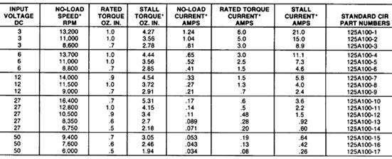
Here

The `input voltage’ is the recommended voltage V to apply to the motor. All other data in the table assume that the motor is used with this voltage. If you wish, you can run a motor with a lower voltage (this will make it run more slowly) and if you are feeling brave you can increase the voltage slightly but this might cause it to burn out, invalidate your warranty and expose you to a potential lawsuit from your customers…
The `No load speed’ is the speed of the motor when it is spinning freely with T=0
The `No load current’ is the corresponding current
The `Stall torque’ is the value of T when the motor is not spinning
The ‘Stall current’ is the corresponding current
The `rated torque’ and `rated current’ are limits to the steady running of the motor the torque and current should not exceed these values for an extended period of time.

The values in the table can be substituted into the formulas relating current, voltage, torque and motor speed, which yield four equations for the unknown values of R,

and

Solving these equations gives

HEALTH WARNING: When you use these formulas it is critical to use a consistent set of units. SI units are very strongly recommended! Volts and Amperes are SI units of electrical potential and electric current. But the torques must be converted into Nm. The conversion factor is 1 ‘oz-in’ is 0.0070612 Nm.

Not all motor manufacturers provide such detailed specifications

it is more common to be given (i) the stall torque; (ii) the no load speed; and (iii) the stall current. If this is the case you have to assume

and take

. If you aren’t given the stall current you have to take

as well.

Power Curves for a brushed electric motor driven from a constant voltage power supply: The rate of work done by the motor is

. The power can be calculated in terms of the angular speed of the motor as

The power curve is sketched in the figure. The most important features are (i) The motor develops no power at both zero speed and the no load speed; and (ii) the motor develops its maximum power

at speed

Efficiency of a brushed electric motor: The electrical power supplied to a motor can be calculated from the current Iand voltage V as

. The efficiency can therefore be calculated as

The second expression can be used to calculate the speed that maximizes efficiency.

Power transmission in machines

A machine is a system that converts one form of motion into another. A lever is a simple example

if point A on the lever is made to move, then point B will move either faster or slower than A, depending on the lengths of the two lever arms. Other, more practical examples include

Your skeleton; used to help convert muscle motion into various more useful forms…
The transmission of a vehicle used to convert rotational motion induced by the engine’s crank-shaft to translational motion of the vehicle
A gearbox converts rotational motion at one angular speed to rotational motion at another.
A system of pulleys.

Concepts of work and energy are extremely useful to analyze transmission of forces and moments through a machine. The goal of these calculations is to quickly determine relationships between external forces acting on the machine, rather than to analyze the motion of the system itself.

To do this, we usually make two assumptions:

The machine is a conservative system. This is true as long as friction in the machine can be neglected.
The kinetic and potential energy of the mechanism within the machine can be neglected. This is true if either (i) the machine has negligible mass and is very stiff (i.e. it does not deform); or (ii) the machine moves at steady speed or is stationary.

If this is the case, the total rate of work done by external forces acting on the machine is zero. This principle can be used to relate external forces acting on the machine, without having to work through the very lengthy and tedious process of computing all the internal forces.

The procedure to do this is always:

Derive a relationship between the velocities of the points where external forces act this is always a geometric relationship.
Write down the total rate of external work done on the system
Use (1) and (2) to relate the external forces to each other.

The procedure is illustrated using a number of examples below.

Example 1: As a first example, we derive a formula relating the forces acting on the two ends of a lever. Assume that the forces act perpendicular to the lever as shown in the figure.

Calculation

Suppose that the lever rotates about the pivot at some angular rate .
The ends of the lever have velocities (see the circular motion example in the preceding chapter if you can’t remember how to show this.
The force vectors can be expressed as
The reaction forces at the pivot are stationary and so do no work.
The total rate of work done on the lever is therefore

The rate of external work is zero, so

Example 2: Here we revisit an EN3 statics problem. The rabbit uses a pulley system to raise carrot with weight W. Calculate the force applied by the rabbit on the cable.

The velocity of the end of the cable held by the rabbit is , with direction parallel to the cable
The velocity of the carrot is ; its direction is vertical
The total length of the cable (aside from small, constant lengths going around the pulleys) is . Since the length is constant, it follows that

The external forces acting on the pulley system are (i) the weight of the carrot W, acting vertically; (ii) the unknown force F applied by the rabbit, acting parallel to the cable; and (iii) the reaction force acting on the topmost pulley. The rate of work done by the rabbit is , the rate of work done by the gravitational force acting on the carrot is . The reaction force is stationary, and so does no work. The total rate of work done is therefore

Using (3) and (4) we see that

Example 3 Calculate the torque that must be applied to a screw with pitch d in order to raise a weight W.

Here, we regard the screw as a machine subjected to external forces.

When the screw turns through one complete turn ( radians) it raises the weight by a distance d
The work done by the torque is ; the work done by the weight is Wd. The reaction forces acting on the thread of the screw do no work
The total work is zero, therefore .

Example 4: A gearbox is used for two purposes: (i) it can amplify or attenuate torques, or moments; and (ii) it can change the speed of a rotating shaft. The characteristics of a gearbox are specified by its gear ratio specifies the ratio of the rotational speed of the output shaft to that of the input shaft

The sketch shows an example. A power source (a rotational motor) drives the input shaft; while the output shaft is used to drive a load. The rotational motion of the input and output shafts can be described by angular velocity vectors

(note that the shafts don’t necessarily have to rotate in the same direction

if they don’t then one of

will be negative).

A quick power calculation can be used to relate the moments

acting on the input and output shafts.

The gear ratio relates the input and output angular velocities as
The rate of work done on the gearbox by the moment acting on the input shaft is . The work done by the moment acting on the output shaft is . A reaction moment must act on the base of the gearbox, but since the gearbox is stationary this reaction moment does no work.
The rate of work done by all the external forces on the gearbox is zero, so

Example 5: Find a formula for the engine power required for a vehicle with mass m to climb a slope with angle

at speed v. Estimate values for engine power required for various vehicles to climb a slopes of 3%, 4% and 5% (these are typical standard grades for flat, rolling and mountain terrain freeways, see, e.g. the Roadway Engineering Highway Design Manual for Oregon at Also, estimate (a) the torque exerted by the engine crankshaft on the transmission; and (b) the force acting on the pistons of the engine.

Assumptions:

The only forces acting on the vehicle are aerodynamic drag, gravity, and reaction forces at the driving wheels.
Aerodynamic drag will be assumed to be in the high Reynolds number regime, with a drag coefficient of order
The crankshaft rotates at approximately 2000rpm.
As a representative examples of engines, we will consider (i) a large 6 cylinder 4 stroke diesel engine, with stroke (distance moved by the pistons) of 150mm; and (ii) a small 4 cylinder gasoline powered engine with stroke 94mm

Calculation. The figure shows a free body diagram for the truck. It shows (i) gravity; (ii) Aerodynamic drag; (iii) reaction forces acting on the wheels.

The velocity vector of the vehicle is
The rate of work done by the gravitational and aerodynamic forces is

where

, with

the drag coefficient, A the frontal area of the vehicle, and

the air density.

The reaction forces acting on the wheels do no work, because they act on stationary points (the wheel is not moving where it touches the ground).
The kinetic energy of the vehicle is constant, so the total rate of work done on the vehicle must be zero. The moving parts of the engine (specifically, the pressure acting on the pistons) do work on the vehicle. Denoting the power of the engine by , we have that

The torque exerted by the crankshaft can be estimated by noting that the rate of work done by the engine is related to the torque T and the rotational speed of the crankshaft by . The torque follows as
The force F on the pistons can be estimated by noting that the rate of work done by a piston is related to the speed of the piston v by . In a four-stroke engine, each piston does work 25% of the time (during the firing stroke). If the engine has n cylinders, the total engine power is therefore . Finally, the piston speed can be estimated by noting that the piston travels the distance of the stroke during half a revolution, and so has average speed . This shows that .

The table below calculates values for two examples of vehicles

Vehicle	Grade	Weight (kg)	Frontal area	Drag Coeft	Speed m/s	Engine speed Rad/sec	Stroke m	Engine power Watts	Torque Nm	Piston force N
18 wheeler	3%	36000	10	0.1	29	12600	0.15	320000	25	355
	4%							420000	34	470
	5%							520000	42	580
Chevy cobalt	3%	1250	2.5	.1	29	12600	0.095	14000	1.1	36
	4%							17000	1.4	46
	5%							21000	1.7	55

XXX . ___ . 000 Concept Lead screw on energy for Transmission

A leadscrew (or lead screw), also known as a power screw or translation screw, is a screw used as a linkage in a machine, to translate turning motion into linear motion. Because of the large area of sliding contact between their male and female members, screw threads have larger frictional energy losses compared to other linkages. They are not typically used to carry high power, but more for intermittent use in low power actuator and positioner mechanisms. Common applications are linear actuators, machine slides (such as in machine tools), vises, presses, and jacks.

Leadscrews are manufactured in the same way as other thread forms (they may be rolled, cut, or ground).

A lead screw is sometimes used with a split nut also called half nut which allows the nut to be disengaged from the threads and moved axially, independently of the screw's rotation, when needed (such as in single-point threading on a manual lathe).

A mechanical linkage is an assembly of bodies connected to manage forces and movement. The movement of a body, or link, is studied using geometry so the link is considered to be rigid. The connections between links are modeled as providing ideal movement, pure rotation or sliding for example, and are called joints. A linkage modeled as a network of rigid links and ideal joints is called a kinematic chain.

Three types of screw thread used in lead screws:
3 & 4: buttress thread
5: round thread
6: square thread

DVD drive with lead screw and stepper motor.

Types

Power screws are classified by the geometry of their thread. V-threads are less suitable for lead screws than others such as ACME because they have more friction between the threads. Their threads are designed to induce this friction to keep the fastener from loosening. Lead screws, on the other hand, are designed to minimize friction. Therefore, in most commercial and industrial use, V-threads are avoided for lead screw use. Nevertheless, V-threads are sometimes successfully used as lead screws, for example on microlathes and micromills.

Square thread

Square threads are named after their square geometry. They are the most efficient, having the least friction, so they are often used for screws that carry high power. But they are also the most difficult to machine, and are thus the most expensive.

Acme thread

An Acme screw

Acme threads have a 29° thread angle, which is easier to machine than square threads. They are not as efficient as square threads, due to the increased friction induced by the thread angle. ACME Threads are generally also stronger than square threads due to their trapezoidal thread profile, which provides greater load-bearing capabilities.

Buttress thread

Buttress threads are of a triangular shape. These are used where the load force on the screw is only applied in one direction. They are as efficient as square threads in these applications, but are easier to manufacture.

Advantages & disadvantages

Leadscrews are used to raise and lower the front door of the Boeing 747-8F Freighter aircraft.

The advantages of a lead screw are:

Large load carrying capability
Compact
Simple to design
Easy to manufacture; no specialized machinery is required
Large mechanical advantage
Precise and accurate linear motion
Smooth, quiet, and low maintenance
Minimal number of parts
Most are self-locking

The disadvantages are that most are not very efficient. Due to the low efficiency they cannot be used in continuous power transmission applications. They also have a high degree of friction on the threads, which can wear the threads out quickly. For square threads, the nut must be replaced; for trapezoidal threads, a split nut may be used to compensate for the wear.

Alternatives

Alternatives to actuation by lead screw include:

Ball screws and roller screws (sometimes categorized as types of leadscrew rather than in contradistinction)
Fluid power (i.e., hydraulics and pneumatics)
Gear trains (e.g., worm drives, rack-and-pinion drives)
Electromagnetic actuation (e.g., solenoids)
Piezoelectric actuation

Mechanics

Diagram of an "unwrapped" screw thread

The torque required to lift or lower a load can be calculated by "unwrapping" one revolution of a thread. This is most easily described for a square or buttress thread as the thread angle is 0 and has no bearing on the calculations. The unwrapped thread forms a right angle triangle where the base is

\pi d_{m}

long and the height is the lead (pictured to the right). The force of the load is directed downward, the normal force is perpendicular to the hypotenuse of the triangle, the frictional force is directed in the opposite direction of the direction of motion (perpendicular to the normal force or along the hypotenuse), and an imaginary "effort" force is acting horizontally in the direction opposite the direction of the frictional force. Using this free-body diagram the torque required to lift or lower a load can be calculated:

T_{raise}={\frac {Fd_{m}}{2}}\left({\frac {l+\pi \mu d_{m}}{\pi d_{m}-\mu l}}\right)={\frac {Fd_{m}}{2}}\tan {\left(\phi +\lambda \right)}

T_{lower}={\frac {Fd_{m}}{2}}\left({\frac {\pi \mu d_{m}-l}{\pi d_{m}+\mu l}}\right)={\frac {Fd_{m}}{2}}\tan {\left(\phi -\lambda \right)}

Coefficient of friction for lead screw threads
Screw material	Nut material
Screw material	Steel	Bronze	Brass	Cast iron
Steel, dry	0.15–0.25	0.15–0.23	0.15–0.19	0.15–0.25
Steel, machine oil	0.11–0.17	0.10–0.16	0.10–0.15	0.11–0.17
Bronze	0.08–0.12	0.04–0.06	-	0.06–0.09

where

T = torque
F = load on the screw
d_m = mean diameter
$\mu \,$ = coefficient of friction (common values are found in the adjacent table)
l = lead
$\phi \,$ = angle of friction
$\lambda \,$ = lead angle

Based on the T_lower equation it can be found that the screw is self-locking when the coefficient of friction is greater than the tangent of the lead angle. An equivalent comparison is when the friction angle is greater than the lead angle (

\phi >\lambda

). When this is not true the screw will back-drive, or lower under the weight of the load.

The efficiency, calculated using the torque equations above, is:

{\mbox{efficiency}}={\frac {T_{0}}{T_{raise}}}={\frac {Fl}{2\pi T_{raise}}}={\frac {\tan {\lambda }}{\tan {\left(\phi +\lambda \right)}}}

For screws that have a thread angle other than zero, such as a trapezoidal thread, this must be compensated as it increases the frictional forces. The equations below take this into account:

T_{raise}={\frac {Fd_{m}}{2}}\left({\frac {l+\pi \mu d_{m}\sec {\alpha }}{\pi d_{m}-\mu l\sec {\alpha }}}\right)={\frac {Fd_{m}}{2}}\left({\frac {\mu \sec {\alpha }+\tan {\lambda }}{1-\mu \sec {\alpha }\tan {\lambda }}}\right)

T_{lower}={\frac {Fd_{m}}{2}}\left({\frac {\pi \mu d_{m}\sec {\alpha }-l}{\pi d_{m}+\mu l\sec {\alpha }}}\right)={\frac {Fd_{m}}{2}}\left({\frac {\mu \sec {\alpha }-\tan {\lambda }}{1+\mu \sec {\alpha }\tan {\lambda }}}\right)

where

\alpha \,

is one half the thread angle.

If the leadscrew has a collar in which the load rides on then the frictional forces between the interface must be accounted for in the torque calculations as well. For the following equation the load is assumed to be concentrated at the mean collar diameter (d_c):

T_{c}={\frac {F\mu _{c}d_{c}}{2}}

where

\mu _{c}

is the coefficient of friction between the collar on the load and d_c is the mean collar diameter. For collars that use thrust bearings the frictional loss is negligible and the above equation can be ignored.

Coefficient of friction for thrust collars
Material combination	Starting $\mu _{c}$	Running $\mu _{c}$
Soft steel / cast iron	0.17	0.12
Hardened steel / cast iron	0.15	0.09
Soft steel / bronze	0.10	0.08
Hardened steel / bronze	0.08	0.06

Running speed

Safe running speeds for various nut materials and loads on a steel screw
Nut material	Safe loads [psi]	Speed
Bronze	2500–3500	Low speed
Bronze	1600–2500	10 fpm
Cast iron	1800–2500	8 fpm
Bronze	800–1400	20–40 fpm
Cast iron	600–1000	20–40 fpm
Bronze	150–240	50 fpm

The running speed for a leadscrew (or ball screw) is typically limited to, at most, 80% of the calculated critical speed. The critical speed is the speed that excites the natural frequency of the screw. For a steel leadscrew or steel ballscrew, the critical speed is approximately

N={(4.76\times 10^{6})d_{r}C \over L^{2}}

where

N = critical speed in RPM
d_r = smallest (root) diameter of the leadscrew in inches
L = length between bearing supports in inches
C = .36 for one end fixed, one end free
C = 1.00 for both ends simple
C = 1.47 for one end fixed, one end simple
C = 2.23 for both ends fixed

Fine adjustment screw

100 TPI Threaded Screw

The term fine adjustment screw typically refers to screws with threads from 40-100 TPI (Threads Per Inch) (0.5mm to 0.2mm pitch) and ultra fine adjustment screw has been used to refer to 100–508 TPI (0.2–0.05 mm pitch). Even though these are non-standard threads, both ISO metric screw thread designations and UNC designations have been used to call out thread dimensions and fit (class). A typical use for a fine adjustment screw is in an optical mirror mount as an adjuster. Typically 80 TPI screws are used in mirror mounts. Ultra fine adjuster screws are used in applications requiring extremely fine motion like laser alignment, fiber coupling.

Fine and ultra fine adjustment screws are often used in photonics applications as part of purchased equipment (i.e. mirror mounts) or built into lab made (home built) apparatus. Often, screws are purchased with matching bushings to be integrated into an experiment or commercial product once attained. Fine adjustment screws and mirror mounts are available as standard items from most companies that sell optics hardware.

Explanation

The fine motion can most easily be calculated by using the pitch or TPI to determine how many micro metres per revolution the screw moves. The table below shows some common examples

TPI (Threads per Inch)	Pitch (in/revolution)	Pitch (mm/revolution)	Pitch (µm/revolution)
40	0.0250	0.635	635
80	0.0125	0.318	318
100	0.0100	0.254	254
127	0.0079	0.200	200
200	0.0050	0.127	127
254	0.0039	0.100	100
508	0.00197	0.050	50

The screw turns 360° in one revolution and with well made screws (minimal stiction) and a user with a sensitive touch, 1° movements can be achieved. Thus, with the ultra fine adjusters sub-micro metre motions are attainable.

Materials

Screws

The material of choice for producing these screws is stainless steel typically 18-8 (303). At the tip of the screw most commonly a stainless steel ball is either pressed or glued into place to provide a single point contact for the surface being moved. Common usage has shown the glue method of attaching the ball to be troublesome in many applications as some commonly used glues (Super Glue) tend to outgas and degrade over time in this application.

Nut/bushing

Each screw requires a nut/bushing which is critical in not only the length and class of the nut/busing but also the material itself. In low cost adjusters where grease can be used and wear and load is small, brass is typically the most economical material to use. In High-end adjusters where tight tolerances are required as well as the capability to withstand wear and higher load, phosphor bronze is the preferred material. Phosphor bronze is considered a self-lubricating material that makes it ideal for grease free applications e.g. vacuum. Still, the use of grease will extend the lifetime of the nut/bushing and is recommended unless a grease free version is required.

Finer adjusters

It is difficult to make screw threads finer than about 250 TPI. As of 2015 only a small handful of companies have the ability to consistently construct threads this fine. For applications that require still finer control, other solutions have been introduced:

Differential adjusters - These adjusters attain a smaller motion than possible from one thread alone by using the difference between the motions of two nuts moving simultaneously along two different thread pitches on one axle. There are many commercially available versions of these at prices from many times that of the fine threads and bushing alone. With this solution backlash is often a problem as backlash from the two threads combines additively.
Sub-micron Adjusters - These use a lever configuration or cone configuration to de-amplify the motion of a screw. These can be engineered to minimize backlash. Prices are similar to differential adjusters.

How a Lead Screw Works

A lead screw turns rotary motion into linear motion combining a screw and a nut where the screw thread is in direct contact with the nut thread. In the case of roller screws, the rollers rather than the nut are in direct contact with the screw thread offering greater efficiency.

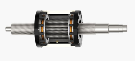
In the case of roller screws, the rollers rather than the nut are in direct contact with the screw thread offering greater efficiency. There are three types of manufacturing process for a screw, either rolled, ground or machined using a whirling process. Power Jacks employs all methods in the manufacture of our lead screws.

Lead screws are used in a very broad range of applications, sold as individual products or incorporated into screw jacks and electro-mechanical actuators. As with screw jacks, Industrial Automation, Medical, Defence and Transport applications are particularly popular lead screws.

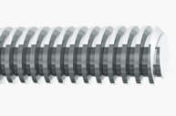
Through both our experience and machining capabilities, Power Jacks have the ability to offer may thread forms customised to suit your application, multi starts, variable pitch treads, diameter to 300mm and lengths up to 20 metres.

Trapezoidal thread
Sharp thread
Buttress thread
Knuckle thread
Course thread
Diamond thread
Threaded nuts
Lead screw repair & reverse engineering

How a Screw Jack Works

A screw jack is a gearbox assembly (either worm gear or bevel gear) and a transmission product (lead screw, ball screw or roller screw) which through use of a motor is used to convert rotary into linear motion. They can be used to push, pull, tension, lock, unlock, tilt, pivot, roll, slide and lift or lower loads, anything from a few kilos to thousands of tonnes.

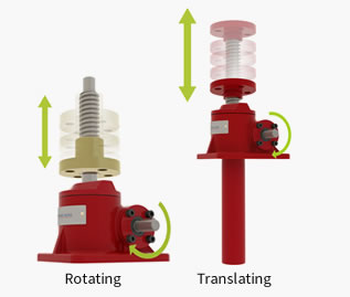
Screw jacks are essential components in automated machinery. Safety and legislative concerns drive the automation of handling and lifting of heavy loads, particularly in regions which have developed workplace and health and safety legislation.

The trend to electromechanical actuation from hydraulic actuation.

Screw jacks usually operate in high-load applications. The competing technology at high loads tends to be hydraulics; however, hydraulics are less energy-efficient than electro-mechanical actuation provided by screw jacks. Hydraulic systems waste energy as the fluid circulates at constant pressure, regardless of the amount of work required to be carried out by hydraulic positioning. A hydraulic jack or ram requires a constant pressure to maintain its position when holding a load in place. By contrast, an electric motor used to power a screw jack uses energy only when it drives the load to a required position.

The advantages of electro-mechanical over hydraulic can be summarized by:

Demand for increased safety, in the event of power loss, screw jacks can be self locking
Demand for machinery that operates with better energy efficiency
Demand for machinery that operates greater levels of precision
Machinery that requires less maintenance
Machinery that requires less manual intervention to set up processes
Increased range of actuation in terms of variable positioning
Accurate and smooth delivery of force
Cleaner machinery .

Linear Actuators

A linear actuator is a device that moves between two points in a linear motion. Linear actuators are available based on a variety of technologies including: Mechanical, Electro-Mechanical, Direct Electric (Linear Motors), Hydraulic & Pneumatic.

All of Power Jacks linear actuators are either mechanical or electro-mechanical. Electro-Mechanical Linear actuators are also known as Electric Linear Actuators due to the primary drive being an electric motor.

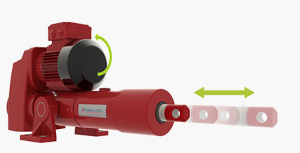
Electric Linear Actuators (ELA) convert the rotary motion of the electric motor to linear motion by means of two main components a gearbox (rotary motion) and a lead screw (linear motion). There are 3 types of lead screws used in our electric linear actuators: Machine Screw, Ball Screw & Roller Screw.

The electric motors rotation drives the primary gear of the gearbox, which through single or multiple gear stages turns the gearboxes output shaft (final gear). This rotates in unison with the lead screw. When the lead screw rotates the lead nut that mates with the lead screw translates along the screw and so converts rotary motion to linear motion.

When compared to Screw Jacks the Electric Linear Actuators offer a pre-packaged actuator with full lead screw protection (fully enclosed inside ram), integrated electric motor, integrated mounting options and control feedback devices.

The Electric Linear Actuators are suitable for low to high duty applications in most industry sectors and offer a better solution than hydraulic and pneumatic actuators in most cases.

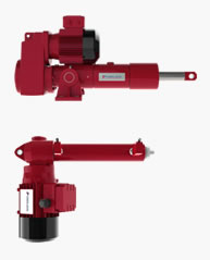
How a Bevel Gearbox Works

A bevel gearbox is a device used to transmit and/or split/distribute the power of a singular rotating mechanical drive shaft through a defined angle, typically 90°.

Though most bevel gearboxes operate at 90° angles other angles are also available, both acute (less than 90°) and obtuse (greater than 90°).

The name bevel gearbox is derived from the gear design used inside the gearbox i.e. bevel gears. The gearboxes are a single stage unit typically supplied with gear ratios within a range from 1:1 to 4:1. They can be supplied in fractional gear ratios as well e.g. 1.5:1.

Bevel gearboxes are ideal when a drive line needs to turn a corner or one drive line needs to power multiple devices from one motor. For example a series of driven rollers on a car production line all driven from 1 motor with each roller at 90° to the main drive shaft and each roller connecting into the main drive shaft via a bevel gearbox.

Screw Jack Systems are another ideal use for Bevel Gearboxes and this is why the product fit neatly into Power Jacks product portfolio. The bevel gearboxes allow Power Jacks to mechanically distribute the power from 1 motor to multiple screw jacks via drive shafts and bevel gearboxes.

We have a long history in the design and manufacture of gearboxes which was reinforced in 2002 when we acquired Neeter Drive the UK’s largest manufacturer of bevel gearboxes. Our gearboxes are extensively specified in applications where compactness, reliability, efficiency and low noise are required. Our speciality is in the ability to offer customers, in addition to standard designs, special designs and adaptations that allow customers to get the best solution for a given application. This includes alternate gear ratios (e.g. 1.46:1), different shaft angles, special materials and special sealing & lubrication. This is why the gearboxes are seen used in a wide variety of applications whether in factories, nuclear plants, offshore, subsea, defence, food processing, metal production, automotive and renewables.

How a Jacking System Works

A screw jack system is where more than one screw jack is operated in unison to achieve a linear movement. The screw jack system arrangement is also commonly referred to as a “jacking system”.

The ability to mechanically link multiple screw jacks together so that they move in unison is one of their greatest advantages. Typical arrangements involve screw jacks, bevel gear boxes, motors, reduction gearboxes, drive shafts, couplings and plummer blocks.

Jacking Systems have 2 main features:

They allow for the movement of large loads driven by a single motor e.g. 4 x ME18100 screw jacks arranged in a screw jack system could move a load of 400 Te (4000kN).
Support loads evenly over a relatively large surface area e.g. 20Te load over a 24m2 area using four screw jacks with 6m x 4m centre spacing.

Typically jacking systems are mechanically linked between each driven item in the system. However electronically linked systems are also available. In these systems the screw jacks are individually motorised and synchronised via an electronic control system and closed feedback loop. This can also be expanded so that multiple mechanically linked jacking systems are synchronised / controlled electronically allowing linear motion solutions to be provided on a massive scale.

This has allowed Power Jacks to provide jacking system solutions into most sectors. Production type environments whether in metal, civil, automotive, paper or energy are the main users of jacking systems however applications such as stadiums, communications and research also use jacking systems of small and large designs.

Load Monitoring

A division of Power Jacks devoted to Load Monitoring Solutions.

We manufacture a comprehensive range of standard load cell products and also offer a bespoke, custom load cell design service. In addition to the load cell products we offer a hire, repair and calibration service.

Load Pins

Suitable for all industry sectors including Construction, Factory Automation, Marine, Offshore and Subsea.

Accurate real time load monitoring of any load bearing pin connection or joint.
Standard capacities from 2Te to 2000Te.
Load Pins designed to exactly suit your application.
Robust, Compact, High Tensile Stainless Steel design.
Accuracy to 1%
Proof Load 150%
Safety Factor of 5:1
Output options include mV, mA, V, RS232 with others available (on request)
Single, Dual and Redundant Bridge Designs
Wireless and cabled options available.
Axial or radial cable exit.
Standard cabled versions have glanded exit with 5m flying cable.
Plugin Connector versions available.
Integral signal conditioning available.
Enclosure IP67 as standard.
ATEX version available for Zones 0, 1 and 2.
Every unit load tested and certified.

Compressive Load Cells

Ideally suited to accurate compressive force measurement in harsh conditions.
Capacities from 2Te to 1000Te as standard.
Cells designed to exactly suit your application.
Robust, Compact, Stainless Steel design.
Accurate to better than 1%
Proof Load 200% (LOLER Compliant)
Safety Factor of 5:1
Supplied with domed top and spherical loading cap.
Operating Temperature -20°C to +80°C as standard.
Enclosure IP67 rated.
Every unit load tested and certified.
Wireless and cabled options available.
ATEX version available for Zones 0, 1 and 2.
ATEX Zone 0 available as cable only design.
Subsea variants available on request.

Load Links

Accurate and reliable tensile load monitoring for lifting applications.
Suitable for all industry sectors including Marine, Offshore and Subsea.
Ideal for mobile applications and services.
Retro-fit load monitoring to existing applications where shackles already available
Wireless and Cable versions

Load Shackles

For compact, reliable and precise tensile load monitoring for your lifting, pulling or weighing applications.
Suitable for all industry sectors including Marine, Offshore and Subsea.
14 Load Shackle designs from 2Te to 500Te as standard
Up to 2000Te Load Shackles available on request
Robust, Compact, High Tensile Steel design using high grade material
Internal Antenna on all wireless models
Design uses VanBeest™ Greenpin® shackles as standard. Others on request
Load pins from high strength stainless steel
Safety Factor of 5:1
Wireless and cabled options available
Cabled versions have a long 15m flying cable as standard
Matched handheld telemetry display
Up to 12 shackles can be linked to the handheld display for individual or summed load values
Data logging software available
Integral signal conditioning
ATEX versions available
Every unit (shackle and load pin) load tested and certified
Special design available on request

Running Line Tensiometer

For winch, crane, tow, laying and tensioning applications
20 Running Line Tensiometer designs
Line Diameters from Ø10mm to Ø100mm
Line Capacities up to 120Te
Rugged design for operation in the most extreme environments
Simple and quick access for line/rope fitting
Hazardous area ATEX models available for all environments
Marinised design ensures corrosion prevention in Offshore environments.
Line mounted supplied with tether/swivel mount as standard with the options for bolt on feet or trunnion mount (pivot on 2 feet)
Custom mounts available on request.
Wireless options available
Data logging software available

Load Cell Displays

Advanced handheld displays with models that allow up to 12 load monitoring devices to be displayed on one unit.
Wireless or cabled designs.
Wireless units use worldwide licence exempt 2.4 GHz radio
Low power consumption for longer battery life on handheld displays.
Rugged fixed display with options for ATEX rated units
Calibrated in Tonne with kg resolution accuracy
Simple to use keypad with multidigit 9mm LCD display.
RS232 output available.
Matched for use with Power Jacks Load Monitoring Solutions

Data Logging

All Wireless Units can be transmitted to Local PC for immediate displaying on screen.
Live logging and graph display
Exportable to Excel
User can plot graph, capture peak loads and analyse test for producing to end clients and test presentations.
MS Windows based
Standard product uses descrete USB powered Base station so that no hardware installation required

Load Cell Services

Benefit from the Load Monitoring experts and our state of the art facilities where we design, manufacture, service and test load monitoring equipment.

Compliance with all major standards including those for LOLER, BSI, DNV, ASME, CE, EMC, FCC, Machinery Directive.

Services include:

Calibration
Repair
Inspection
Non-Destructive Testing (including over-load and proof-load)
Certification
Upgrade electronics
Upgrade for strain gauges
Conversions (eg cabled to wireless)
New Electronics for existing products
Analogue and digital output module upgrades
Bespoke Test Reports
Stress Analysis and Measurement for client products whether in-service or in laboratory

XXX . ___ . 000 223 This Is How An Automatic Transmission Works

Ever wonder how your transmission knows to shift gears? Why is it that when you stop, the engine doesn't die? We're here to show you how cars work. We recently looked at manual transmissions. This week it's regular ol' slushbox time.

Automatic transmissions – they're pretty much black magic. The sheer number of moving parts makes them very difficult to comprehend. Let's simplify it a bit to get a basic understanding of how it all works in a traditional, torque converter-based system.

Your engine connects to your transmission at a place called a bell housing. The bell housing contains a torque converter for automatic transmission-equipped vehicles as opposed to a clutch on manual vehicles. The torque converter is a fluid coupling whose job it is to connect your engine to your transmission and thus to your driven wheels. The transmission contains planetary gearsets which are in charge of providing different gear ratios. To get a good understanding of how the whole automatic transmission system works, let's have a look at torque converters and planetary gearsets.

First and foremost, your engine's flex plate (basically a flywheel for an automatic) connects directly to a torque converter. So when the crankshaft rotates, so does the torque converter housing. The goal of the torque converter is to provide a means by which to connect and disconnect the engine's power to the driven load. The torque converter takes the place of a clutch on a conventional manual transmission. How does the torque converter work? Well, have a look at the video above. It explains the basic principles behind a fluid coupling. Once you've watched that, continue reading to see how a torque converter differs from a standard fluid coupling.

The major components of a torque converter are: the impeller, the turbine, the stator, and the lock-up clutch. The impeller is part of the torque converter housing, which is connected to the engine. It drives the turbine via viscous forces. The turbine is connected to the transmission input shaft. In essence, the engine turns the impeller which imparts forces on a fluid, which then rotates the turbine, sending torque to the transmission.

The transmission fluid flows in a loop between the impeller to the turbine. The fluid coupling in the video above suffers from severe churning losses (and consequent heat buildup) as the fluid returning from the turbine has a component of its velocity that opposes the rotation of the impeller. That is, the fluid returning from the turbine works against the impeller's rotation and thus against the engine.

The stator sits between the impeller and turbine. Its goal is to minimize churning losses and to increase torque output by redirecting the fluid as it returns from the turbine to the impeller. The stator directs the fluid so that the majority of its velocity is in the direction of the impeller, helping the impeller move, and thus adding to the torque produced by the motor. This ability to multiply torque is why we call them torque converters, not fluid couplings.

The stator sits on a one-way clutch. It can rotate in one direction only when the turbine and impeller are moving at approximately the same speed (like during highway driving). The stator either rotates with the impeller or not at all. Stators don't always multiply torque, though. They provide you with more torque when you're either at stall (applying the brakes at a stop light, for example) or while accelerating, but not during highway cruising.

In addition to the one-way clutch in the stator, some torque converters contain a lock-up clutch whose job it is to lock the turbine with the torque converter housing so that the turbine and impeller are mechanically connected. Eliminating the fluid coupling and replacing it with a mechanical connection ensures that all of the engine's torque is transmitted to the transmission input shaft.

Planetary Gears

So, now that we've figured out how the engine sends power to the transmission, it's time to figure out how in tarnation it changes gears. On a conventional transmission, changing gears is the job of a compound planetary gear set. Understanding how planetary gear sets work is a bit tricky, so let's have a look at a basic planetary gear set.

A planetary gearset (also known as an epicyclic gear set) consists of a sun gear in the center, planet gears that rotate around the sun gear, a planet carrier that connects the planet gears, and a ring gear on the outside that meshes with the planet gears. The basic idea behind a planetary gear set is this: using clutches and brakes, you can prevent certain components from moving. In doing so, you can alter the input and output of the system and thus change the overall gear ratio. Think of it this way: a planetary gear set lets you change gear ratios without having to engage different gears. They're all already engaged. All you have to do is use clutches and brakes to change which components rotate and which stay stationary.

The final gear ratio depends on which component is fixed. For example, if the ring gear is fixed, the gear ratio will be much shorter than if the sun gear is fixed. Knowing full well the risks associated with ploppin' an equation on here, I'm gonna put one in anyway. The following equation will tell you your gear ratios depending on which component is fixed and which are in motion. R, C, and S represent the ring gear, carrier, and sun gear. Omega simply represents the angular speed of the gears, and N is the tooth count.

The way it works is thus: let's say we decided to keep the planet carrier stationary and make the sun gear our input (thus the ring gear is our output). The planets are able to rotate, but they cannot move since the carrier cannot move. Omega_c is zero, so the left side of the equation above is gone. This means that when we rotate the sun gear, it sends torque through the planet gears to the ring gear. To figure out what the gear ratio would be, we simply solve the above equation for Omega_r/Omega_s. We end up with -N_s/N_R, that is, the gear ratio when we fix the carrier and make the ring gear our output and the sun gear our input is simply the ratio of the number of teeth between the sun gear and ring gear. This is negative, since the ring spins in the opposite direction of the sun gear.

You can also lock the ring gear and make the sun gear your input and you can lock the sun gear and make the carrier your input. Depending on what you lock, you'll get different gear ratios, i.e. you'll get different "gears." To obtain a 1:1 gear ratio, you simply lock the components together (you only have to lock two to do this) so that the crankshaft spins at the same speed as the transmission output shaft.

3 komentar:

Gobiii27 Mei 2018 pukul 23.34
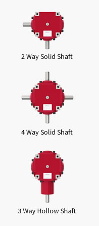
Thanks, for sharing the information, it’s very informative post!

Aluminium Scaffolding Rental In Ahmedabad
BalasHapus
Balasan
GO LOOK IMPORTANTBOOK29 Mei 2018 pukul 22.28
Thankyume too for reading my posting ,and we and the happy family all benefited from our post and can give you the thought and application of the right, true and efficient LJBUSAF

BalasHapus
Balasan

Tambahkan komentar

Selasa, 22 Mei 2018

Electronically Controlled Automatic Transmission (Automobile)