Hasil gambar untuk American flag bearing

Magnetic bearing

A magnetic bearing is a type of bearing that supports a load using magnetic levitation. Magnetic bearings support moving parts without physical contact. For instance, they are able to levitate a rotating shaft and permit relative motion with very low friction and no mechanical wear. Magnetic bearings support the highest speeds of all kinds of bearing and have no maximum relative speed.

Passive magnetic bearings use permanent magnets and, therefore, do not require any input power but are difficult to design due to the limitations described by Earnshaw's theorem. Techniques using diamagnetic materials are relatively undeveloped and strongly depend on material characteristics. As a result, most magnetic bearings are active magnetic bearings, using electromagnets which require continuous power input and an active control system to keep the load stable. In a combined design, permanent magnets are often used to carry the static load and the active magnetic bearing is used when the levitated object deviates from its optimum position. Magnetic bearings typically require a back-up bearing in the case of power or control system failure.

Magnetic bearings are used in several industrial applications such as electrical power generation, petroleum refinement, machine tool operation and natural gas handling. They are also used in the Zippe-type centrifuge, for uranium enrichment and in turbo molecular pumps, where oil-lubricated bearings would be a source of contamination.

A magnetic bearing

Design

Basic operation for a single axis

An active magnetic bearing works on the principle of electromagnetic suspension based on the induction of eddy currents in a rotating conductor. When an electrically conducting material is moving in a magnetic field, a current will be generated in the material that counters the change in the magnetic field (known as Lenz' Law). This generates a current that will result in a magnetic field that is oriented opposite to the one from the magnet. The electrically conducting material is thus acting as a magnetic mirror.

The Hardware consists of an electromagnet assembly, a set of power amplifiers which supply current to the electromagnets, a controller, and gap sensors with associated electronics to provide the feedback required to control the position of the rotor within the gap. The power amplifier supplies equal bias current to two pairs of electromagnets on opposite sides of a rotor. This constant tug-of-war is mediated by the controller, which offsets the bias current by equal and opposite perturbations of current as the rotor deviates from its center position.

The gap sensors are usually inductive in nature and sense in a differential mode. The power amplifiers in a modern commercial application are solid state devices which operate in a pulse width modulation configuration. The controller is usually a microprocessor or digital signal processor.

Active bearings have several advantages: they do not suffer from wear, have low friction, and can often accommodate irregularities in the mass distribution automatically, allowing rotors to spin around their center of mass with very low vibration.

Two types of instabilities are typically present in magnetic bearings. Attractive magnets produce an unstable static force that decreases with increasing distance and increases at decreasing distances. This can cause the bearing to become unbalanced. Secondly, because magnetism is a conservative force, it provides little damping; oscillations may cause loss of successful suspension if any driving forces are present.

Back to Flash Basics

The table below lists several early patents for active magnetic bearings. Earlier patents for magnetic suspensions can be found but are excluded here because they consist of assemblies of permanent magnets of problematic stability per Earnshaw's Theorem.

Early U.S. patents in active magnetic bearings
Inventor(s)	Year	Patent number	Title
Beams, Holmes	1941	2,256,937	Suspension of Rotatable Bodies
Beams	1954	2,691,306	Magnetically Supported Rotating Bodies
Beams	1962	3,041,482	Apparatus for Rotating Freely Suspended Bodies
Beams	1965	3,196,694	Magnetic Suspension System
Wolf	1967	3,316,032	Poly-Phase Magnetic Suspension Transformer
Lyman	1971	3,565,495	Magnetic Suspension Apparatus
Habermann	1973	3,731,984	Magnetic Bearing Block Device for Supporting a Vertical Shaft Adapted for Rotating at High Speed
Habermann, Loyen, Joli, Aubert	1974	3,787,100	Devices Including Rotating Members Supported by Magnetic Bearings
Habermann, Brunet	1977	4,012,083	Magnetic Bearings
Habermann, Brunet, LeClére	1978	4,114,960	Radial Displacement Detector Device for a Magnetic Bearings
Meeks, Crawford R	1992	5,111,102	Magnetic Bearing Structure

Jesse Beams from the University of Virginia filed some of the earliest active magnetic bearing patents during World War II. The patents dealt with ultracentrifuges intended for the enrichment of isotopes of elements needed for the Manhattan Project. However, magnetic bearings did not mature until advances in solid-state electronics and modern computer-based control technology with the work of Habermann and Schweitzer. In 1987, Estelle Croot further improved active magnetic bearing technology, but these designs were not manufactured due to expensive costs of production, which used a laser guidance system. Estelle Croot's research was the subject of 3 Australian patents and was funded by Nachi Fujikoshi, Nippon Seiko KK and Hitachi, and her calculations were used in other technologies that used rare earth magnets but the active magnetic bearings were only developed to the prototype stage.

Kasarda reviews the history of active magnetic bearings in depth. She notes that the first commercial application of active magnetic bearings was in turbomachinery. The active magnetic bearing allowed the elimination of oil reservoirs on compressors for the NOVA Gas Transmission Ltd. (NGTL) gas pipelines in Alberta, Canada. This reduced the fire hazard allowing a substantial reduction in insurance costs. The success of these magnetic bearing installations led NGTL to pioneer the research and development of a digital magnetic bearing control system as a replacement for the analog control systems supplied by the American company Magnetic Bearings Inc. In 1992, NGTL's magnetic bearing research group formed the company Revolve Technologies Inc. for commercializing the digital magnetic bearing technology. The company was later purchased by SKF of Sweden. The French company S2M, founded in 1976, was the first to commercially market active magnetic bearings. Extensive research on magnetic bearings continues at the University of Virginia in the Rotating Machinery and Controls Industrial Research Program

During the decade starting in 1996, the Dutch oil-and-gas company NAM installed twenty gas compressors, each driven by a 23-megawatt variable-speed-drive electric motor. Each unit was fully equipped with active magnetic bearings on both the motor and the compressor. These compressors are used in the Groningen gas field to extract the remaining gas from this large gas field and to increase the field capacity. The motor-compressor design was done by Siemens and the active magnetic bearings were delivered by Waukesha Bearings (owned by Dover Corporation). (Originally these bearings were designed by Glacier, this company was later taken over by Federal Mogul and is now part of Waukesha Bearings.) By using active magnetic bearings and a direct drive between motor and compressor (without having a gearbox in between) and by applying dry gas seals, a fully dry-dry (oil-free) system was achieved. Applying active magnetic bearings in both the driver and in the compressor (compared to the traditional configuration using gears and ball bearings) results in a relatively simple system with a very wide operating range and high efficiencies, particularly at partial load. As was done in the Groningen field, the full installation can additionally be placed outdoors without the need for a large compressor building.

Meeks^[18] pioneered hybrid magnetic bearing designs (US patent 5,111,102) in which permanent magnets provide the bias field and active control coils are used for stability and dynamic control. These designs using permanent magnets for bias fields are smaller and of lighter weight than purely electromagnetic bearings. The electronic control system is also smaller and requires less electrical power because the bias field is provided by the permanent magnets.

As the development of the necessary components progressed, scientific interest in the field also increased, peaking in the first International Symposium on Magnetic Bearings held in 1988 in Zürich with the founding of the International Society of Magnetic Bearings by Prof. Schweitzer (ETHZ), Prof. Allaire (University of Virginia), and Prof. Okada (Ibaraki University). Since then, the symposium has developed into a biennial conference series with a permanent portal on magnetic bearing technology where all symposium contributions are made available.

Magnetic bearing advantages include very low and predictable friction, and the ability to run without lubrication and in a vacuum. Magnetic bearings are increasingly used in industrial machines such as compressors, turbines, pumps, motors and generators.

Magnetic bearings are commonly used in watt-hour meters by electric utilities to measure home power consumption. They are also used in high-precision instruments and to support equipment in a vacuum, for example in flywheel energy storage systems. A flywheel in a vacuum has very low wind resistance losses, but conventional bearings usually fail quickly in a vacuum due to poor lubrication. Magnetic bearings are also used to support maglev trains in order to get low noise and smooth ride by eliminating physical contact surfaces. Disadvantages include high cost, heavy weight and relatively large size.

Magnetic Bearings are also used in some centrifugal compressors for chillers. A shaft made up of magnetic material lies between magnetic bearings. A small amount of current provides magnetic levitation to the shaft which remains freely suspended in air ensuring zero friction between the bearing and the shaft.

A new application of magnetic bearings is in artificial hearts. The use of magnetic suspension in ventricular assist devices was pioneered by Prof. Paul Allaire and Prof. Houston Wood at the University of Virginia, culminating in the first magnetically suspended ventricular assist centrifugal pump (VAD) in 1999.

Several ventricular assist devices use magnetic bearings, including the LifeFlow heart pump, the DuraHeart Left Ventricular Assist System, the Levitronix CentriMag, and the Berlin Heart. In these devices, the single moving part is suspended by a combination of hydrodynamic force and magnetic force. By eliminating physical contact surfaces, magnetic bearings make it easier to reduce areas of high shear stress (which leads to red blood cell damage) and flow stagnation (which leads to clotting) in these blood pumps.

Synchrony Magnetic Bearings, Waukesha Magnetic Bearings, Calnetix Technologies, and S2M are among the magnetic bearing developers and manufacturers worldwide.

Future advances

An axial homopolar electrodynamic bearing

With the use of an induction-based levitation system present in maglev technologies such as the Inductrack system, magnetic bearings could replace complex control systems by using Halbach Arrays and simple closed loop coils. These systems gain in simplicity, but are less advantageous with regard to eddy current losses. For rotating systems it is possible to use homopolar magnet designs instead of multipole Halbach structures, which reduce losses considerably.

An example that has bypassed the Earnshaw's theorem issues is the homopolar electrodynamic bearing invented by Dr Torbjörn Lembke. This is a novel type of electromagnetic bearing based on a passive magnetic technology. It does not require any control electronics to operate and works because the electrical currents generated by motion cause a restoring force.

Active magnetic bearing

Maintenance-Free bearing for maximum speeds

Actuator, sensory components and magnetic bearing electronics from a single source
Complete magnetic bearing motor systems for special and turbo applications
Magnetic bearing electronics can be optimally integrated into a system's drive train
Voltage supply from the drive train possible (incl. grid support)
Suitable for maximum speeds
Active compensation of imbalances

Magnetic bearing motors / generatorsComplete drive solutions for high-speed applications

Optimal solution for blower and turbine applications
Can be used as magnetic bearing motor or generator
Completely maintenance-free
Power: up to 30 kW
Speed: up to 60,000 min-1 (depending on the pressure ratio and the medium)
Bearing force: 1,000 N (radial)
Scope of supply: without impeller
Built-in magnetic bearing electronics for simple and low cost installation
Integrated water cooling

Magnetic bearing spindlesComplete solutions for challenging processing tasks

Magnetic bearing spindle solutions for processing tasks with specific requirements
Power in the multi-kilowatt range
Speeds of up to 60,000 min-1
Automatic tool clamping system
Targeted periodic deflections of the shaft position are possible in radial and axial directions
Integrated minimum lubrication (MQL)

MOTION SYSTEM DESIGN

Dynamic ceramics

Ceramic balls have world-famous surfaces and precision geometry. The inherently strong material can often perform when other materials flake out.

Though increasingly affordable, there’s no getting around that silicon nitride balls are more costly than metal. Luckily, ceramic balls are often used in bearings that are otherwise pretty typical designs. When assembled into a hybrid bearing — ceramic balls in metal races — the price of the bearing assembly is actually quite competitive. On a total operating cost basis, hybrid bearings often pay for themselves many times over in extended life, enhanced performance, or increased durability. Additionally, ceramic balls have become increasingly common over the past fifteen years. As a result, they have steadily become affordable for more applications.

Ceramic bearing balls are made from the structural ceramic called silicon nitride. What makes the material appropriate for ball bearings is its crystalline structure, locked in place with covalent, directional bonds in a diamond-like arrangement. In these directional bonds every atom ionically shares its electrons with its lattice neighborhood. For this reason, ceramics are more loosely packed than metals, and (because they do not react with outside elements to absorb electrons) are electrically nonconductive.

Because they’re also lighter and stiffer, ceramic bearings are capable of higher operating speeds. And, quicker movements make for increased productivity. Another benefit is less required maintenance. The best bearing-grade silicon nitrides have attributes that maximize hardness, crack resistance and rolling contact fatigue life. With tiny (and scarce) pores with maximum diameters under one micron, the material has nearly 100% density. Typically over 85% of grains are in a micron-sized needle-like shape that makes for tough, strong, and fatigue-resistant bearings. Finally, superior rolling contact life (5 times) makes silicon nitride one of the best materials for increasing bearing durability and operational capabilities.

Controlling lube degradation and wear are other areas where ceramics excel. Sometimes frequent startstop cycles, high loads or vibration at low speeds, lack of lubricant, or low viscosity makes for marginally lubricated raceways. Loaded steel balls operating under these conditions quickly accelerate bearing wear. Micro-welding occurs, and micro-fractures of the steel ball and raceways follow. Then surface asperities form, causing metallic wear debris to contaminate the lubricant and degrade its chemistry. The final effect: bearing precision (as measured by vibration, non-repeating run out, and work-piece quality) deteriorates rapidly.

Because micro-welding and fracture does not occur at steel-silicon nitride contact points, ceramic balls help maintain long-term bearing precision. Even when rolling on marginally lubricated steel raceways, ceramic is structurally dissimilar, so adhesive wear is eliminated. Lubricant contamination and degradation is also reduced; smoother ball and raceway surfaces are maintained, resulting in lower internal friction and lower operating temperatures. The synergy of reduced wear and temperature means long-term high precision and extended bearing service life for the end user.

In turn, reduced friction and operating temperatures allow for less lubricant. Here’s why: In typical designs, bearings need lubricant to separate balls from races. The thickness of the lubricant film is determined by factors including speed, bearing size and design, material, and operating temperature. One key guideline for determining the proper thickness of the lubrication layer is the composite surface roughness of the ball and raceway surfaces. In general, the film thickness of the lubricant needs to be 1.5 x CSR. Because ceramic balls have very fine surface finishes, lubricant needs are minimized. Often on hybrid bearings, grease completely replaces oil mist systems. On systems where grease is already specified, the amount used can often be reduced.

Just as other bearing balls, ceramic balls are classified by ABMA, JIS, and ASTM standards. Sphericity, surface finish, lot diameter variation, and other precisely defined factors fall into grade levels. Grade three is typically the highest; this denotes three-millionths sphericity or better. Other grades include five, ten, and so on. Though it is tough to say exactly how much longer hybrid bearings last than steel bearings, generally life is extended two to five times. Because of their inherent lower thermal expansion, smoother surface, increased hardness and corrosion and electrical resistant properties, ceramic balls last longer. It’s true a stiffer ball can increase contact stresses if raceway curvatures are not adjusted. (For extremely high load applications, silicon nitride balls may not be suitable since they may accelerate steel raceway fatigue.) Even so, ceramic balls are not brittle and fragile. While they are not as tough or ductile as steel, they are actually much more durable.

Hybrid roller bearings have longer service life and higher speed capabilities than conventional bearings. Higher speed is achieved in part through the lower density of silicon nitride. At just 40% the density of similar steel rollers, silicon nitride balls offer lower inertia for faster stops and startups. To discuss bearing speed it is necessary to understand the relationship between rpms and the size of the bearing.

DmN = N x Dm

Where DmN = Relative bearing speed pitch diameter

Dm = (Do + Di)/2 = Actual speed

N = Relative speed, rpm

The construct Dm is used to defined relative bearing speed and is given by the pitch diameter (ball path) times the bearing rpm. This dimensionless parameter can be used to compare bearings of different dimensions. Dm is the pitch diameter or ball of the bearing and is determined by the average distance between the outside diameter, Do and the inside diameter, Di, in millimeters. Relative bearing speed, DmN is calculated as the pitch diameter of the bearing multiplied by the speed in rpms. For example, a bearing with a pitch diameter of 10 mm and a speed of 10,000 rpm would have a DmN value of 100,000. A bearing with a pitch diameter of 100-mm bearing is 10 times that of the 10- mm bearing.

Life

Frequently asked is whether load capability affects the L10 life calculation of a hybrid bearing. This is an important issue and has been given significant attention over the past several years. Silicon nitride balls are very stiff, and so the contact patch on the raceway is quite small. For any given load, this means that the stress in the raceway at the contact patch is increased and theoretically the L10 life is reduced in a hybrid bearing. Indeed applications that require bearings to perform at high load levels demonstrate lower life characteristics when a hybrid bearing is substituted for a traditional bearing. Fatiguing is usually to blame. However, if a designer adjusts bearing raceway curvatures and the number of balls, the load-carrying capability can be improved.

Other bearing materials

Chemical makeup is what imparts different characteristics to different bearing balls. For all materials, atoms are everseeking to gain electrical neutrality (with equal number of protons and electrons) to reach the best equilibrium state. Metals are predominantly bonded by non-directional electron sharing between neighboring atoms, known as metallic or electronic bonding. At any moment in time, metal atoms must satisfy only overall electrical neutrality with their surrounding neighborhood; they do not require “ownership” of the electrons surrounding them. Non-directional electron sharing between atoms allows for tightly packed structures (which results in high density) with numerous slip planes (which allows for ductility). Since electrons are not tightly bound to specific neighboring atoms, they are also free to move through the metallic lattice (which results in electrical and thermal conductivity).

Polymers are made of individual molecules attached in long chains at specific, discrete points. Typically, the molecules in a polymer bond are also bound together very tightly. This makes for an interesting combination of properties. Because individual molecules do not allow their electrons to move, corrosion and electrical resistance result. Because the chains can stretch and move within the material, the bonding allows for elasticity and lubricity.

Unlike polymers in chains, ceramics are predominantly bonded by directional bonds between neighboring atoms in expansive lattice structures. Because every atom in a ceramic directionally shares its electrons within its lattice neighborhood through either or both ionic and covalent bonding, ceramics are not tightly packed like metals. Ceramics tend to be very non-reactive or inert because their atoms are essentially electrically neutral through strong directional bonds within a very fixed lattice neighborhood; they have no need to react with surroundings for electrons to satisfy neutrality.

In the wind

Wind energy companies are beginning to realize the advantages of ceramic hybrid bearings, particularly for increasing speed. On a windy day, the blades of a mill can be rotated up to 30 rpm. But to generate electricity, this slower motion of the rotor shaft must be sped up to 2,000 rpm. Bearings that include ceramic balls are beneficial because they eliminate electrical arcing and last longer than steel bearings in these harsh conditions. Challenges include debris and temperature extremes. Maintaining lubricity is also an issue. A long-life bearing is especially attractive because of the high cost of bearing replacement in windmills; a bearing replacement can cost up to $10,000 because of the need for cranes and crews.

Jeff McLaughlin is general manager of Machine Building Specialists of Manitowoc, Wis., a company that provides engineering and manufacturing solutions to the wind turbine, power generation, and construction equipment industries. According to McLaughlin, “the use of hybrid ceramic bearings has helped us achieve and surpass our goals of improved machine performance, reduced maintenance costs, and higher availability for our customers.” Machine Building Specialists use Cerbec ceramic balls in their designs.

“The differential cost over standard bearings is easily justified in wind turbine generator applications, especially for high speed and generator shafting. The lower mass, thermal stability, reduced friction, and electrical isolation — when used as part of a comprehensive remediation plan — have resulted in ‘better-than-new’ OEM performance.”

The birth of a ceramic ball

Like most ceramics, silicon nitride isn’t easily fabricated into single crystals. Instead, silicon nitride balls are polycrystallines with micron-sized, needle-like grains (characterized by acicularity) bonded together by a secondary glassy phase. These two main crystalline polymorphs are called alpha and beta.

1. Through liquid phase sintering by solution-reprecipatation, a sintering aid (usually magnesium or yttrium oxide) forms an inter-granular glass. Alpha silicon nitride dissolves into it, while the beta silicon nitride precipitates out. (Typically the more liquid phase, the lower the temperature and pressure required for densification and microstructural development. But along with that comes increased difficulty to gain appropriate properties for bearing-grade silicon nitride.) Better ceramic varieties possess lower amounts of the liquid phase — under 15 volume percent — and need high temperatures and pressures for enough kinetic and thermodynamic driving force to promote alphato- beta transformation.

2. Ceramic ball fabrication begins with making a pressable powder. Slurry with binders is then spray-dried to make flowable, compactable powder, which is pressed into blanks using uniaxial or isostatic methods. Though other methods do exist, in one common method ball blanks are air-fired to remove binders, loaded into graphite crucibles with encapsulant glass, and hot isostatically pressed at extremely high temperature and pressure. This optimizes densification and microstructure. Both magnesia and yttria-doped materials benefit.

3. At the end of the process, densified ball blanks are de-encapsulated, inspected, and finished. Once qualified for further processing, the balls are roughed and finished in a series of steps utilizing free abrasive lapping with diamond. This is required because silicon nitride is such a hard and tough material.

The sintering aid is the controlling factor concerning corrosion resistance. Both magnesia and yttria-based silicon nitrides are highly inert in most liquids and gases. No organic solvent is known to corrode silicon nitride. In general, magnesia and yttria-based silicon nitrides behave the same in various environments. Some exceptions do exist. For example, yttria-based silicon nitrides are more resistant to hydrofluoric acid solutions than magnesia-based silicon nitrides.

XXX . ____ . 000 COMBINE Hybrid roller bearings have longer service life and higher speed capabilities than conventional bearings. Higher speed is achieved in part through the lower density of silicon nitride. At just 40% the density of similar steel rollers, silicon nitride balls offer lower inertia for faster stops and startups. To discuss bearing speed it is necessary to understand the relationship between rpms and the size of the bearing.

DmN = N x Dm

Where DmN = Relative bearing speed pitch diameter

Dm = (Do + Di)/2 = Actual speed

N = Relative speed, rpm

Life

Special thanks to Saint-Gobain Ceramics for technical information and insight. For more information, visit www.cerbec.com.

Other bearing materials

Continue on page 3

In the wind

The birth of a ceramic ball

XXX . ___ . 000 COMBINE ELECTRON MOTION

The field of electrical theory and electronics is huge, and it can be somewhat daunting at first. In reality, you don’t need to know all the little theoretical details to get things up and running. But to give your efforts a better chance at success, it is a good idea to understand the basics of what electricity is and how, in general terms, it works. So that’s what we’re going to look at here.

The main intent of this chapter is twofold. First, I want to dispense with the old “water-flowing-in-a-pipe” analogy that has been used in the past to describe the flow of electrons in a conductor; it’s not very accurate and can lead to some erroneous assumptions. There is, I believe, a better way to visualize what is going on, but it does require a basic understanding of what an atom is and how its component parts work to create electric charge and, ultimately, electric current. It might sound rather like something from the realm of physics (and, to be honest, it is, along with chemistry), but once you understand these concepts, things like fluorescent lights, neon signs, lightning, arc welders, plasma cutting torches, heating elements, and the electronic components you might want to use in a project will become easier to understand. The old water-flowing-in-a-pipe model doesn’t really scale very well, nor does it translate easily to anything other than, well, water flowing through a pipe.

Second, I’d like to build on this atom-based model to introduce some basic concepts that will come up later as you work on your own projects. By the end of this chapter, you should have a good idea of what the terms voltage, current, and power mean and how to calculate these values. If you need more details on a lower level, you’ll find them in Appendix A, including overviews of serial and parallel circuits, and basic AC circuit concepts. Of course, numerous excellent texts are readily available on the subject, and I encourage you to seek them out if you would like to dig deeper into the theory of electronics.

If you are already familiar with the basic concepts of electronics, feel free to skip this chapter. Just don’t forget to take advantage of Appendix A and the suggested references in Appendix C if you run into a need for further details somewhere along the line.

Atoms and Electrons

In common everyday usage, the term electricity is used to refer to the stuff that one finds inside a computer, in a wall outlet, in the wires strung between poles beside the street, or at the terminals of a battery. But just what is this stuff, really?

Electricity is the physical manifestation of the movement of electrons, little specks of subatomic matter that carry a negative electrical charge. As we know, all matter is composed of atoms. Each atom has a nucleus at its core with a net positive charge. Each atom also has one or more negative electrons bound to it, each one whipping around the positively charged nucleus in a quantum frenzy.

It is not uncommon to hear of the “orbit” of an electron about the nucleus, but this isn’t entirely accurate, at least not in the classical sense of the term orbit. An electron doesn’t orbit the nucleus of an atom in the way a planet orbits a star or a satellite orbits the earth, but it’s a close enough approximation for our purposes.

In reality, it’s more like layers of clouds wrapped around the nucleus, with the electrons being somewhere in the layers of the cloud. One way to think of it is as a probability cloud, with a high probability that the electron is somewhere in a particular layer. Due to the quirks of quantum physics, we can’t directly determine where an electron is located in space at any given time without breaking things, but we can infer where it is by indirect measurements. Yes, it’s a bit mind-numbing, so we won’t delve any deeper into it here. If you want to know more of the details, I would suggest a good modern chemistry or physics textbook, or for a more lightweight introduction, you might want to check out the “Mr. Tompkins” series of books by the late theoretical physicist George Gamow.

The nucleus of most atoms is made up of two basic particles: protons and neutrons, with the exception of the hydrogen atom, which has only a single positive proton as its nucleus. A nucleus may have many protons, depending on what type of atom it happens to be (iron, silicon, oxygen, etc.). Each proton has a positive charge (called a unit charge). Most atoms also have a collection of neutrons, which have about the same mass as a proton but no charge (you might think of them as ballast for the atom’s nucleus). Figure 1-1 shows schematic representations of a hydrogen atom and a copper atom.

The +1 unit charges of the protons in the nucleus will cancel out the –1 unit charges of the electrons, and the atom will be electrically neutral, which is the state that atoms want to be in. If an atom is missing an electron, it will have a net positive charge, and an extra electron will give it a net negative charge.

The electrons of an atom are arranged into what are called orbital shells (the clouds mentioned earlier), with an outermost shell called the valence shell. Conventional theory states that each shell has a unique energy level and each can hold a specific number of electrons. The outermost shell typically determines the chemical and conductive properties of an atom, in terms of how easily it can release or receive an electron. Some elements, such as metals, have what is considered to be an “incomplete” valence shell. Incomplete, in this sense, means that the shell contains fewer than the maximum possible number of electrons, and the element is chemically reactive and able to exchange electrons with other atoms. It is, of course, more complex than that, but a better definition is way beyond the scope of this book.

For example, notice that the copper atom in Figure 1-1 has 29 electrons and one is shown outside of the main group of 28 (which would be arranged in a set of shells around the nucleus, not shown here for clarity). The lone outermost electron is copper’s valence electron. Because the valence shell of copper is incomplete, this electron isn’t very tightly bound, so copper doesn’t put up too much of a fuss about passing it around. In other words, copper is a relatively good conductor.

An element such as sulfur, on the other hand, has a complete outer shell and does not willingly give up any electrons. Sulfur is rated as one of the least conductive elements, so it’s a good insulator. Silver tops the list as the most conductive element, which explains why it’s considered useful in electronics. Copper is next, followed by gold. Still, other elements are somewhat ambivalent about conducting electrons, but will do so under certain conditions. These are called semiconductors, and they are the key to modern electronics.

This should be a sufficient model for our purposes, so we won’t pry any further into the inner secrets of atomic structure. What we’re really interested in here is what happens when atoms do pass electrons around, and why they would do that to begin with.

Electric Charge and Current

Electricity involves two fundamental phenomena: electric charge and electric current. Electric charge is a basic characteristic of matter and is the result of something having too many electrons (negative charge), or too few electrons (positive charge) with regard to what it would otherwise need to be electrically neutral. An atom with a negative or positive charge is sometimes called an ion.

A basic characteristic of electric charges is that charges of the same kind repel one another, and opposite charges attract. This is why electrons and protons are bound together in an atom, although under most conditions they can’t directly combine with each other because of some other fundamental characteristics of atomic particles (the exceptional cases are a certain type of radioactive decay and inside a stellar supernova). The important thing to remember is that a negative charge will repel electrons, and a positive charge will attract them.

Electric charge, in and of itself, is interesting but not particularly useful from an electronics perspective. For our purposes, really interesting things begin to happen only when charges are moving. The movement of electrons through a circuit of some kind is called electric current, or current flow, and it is also what happens when the static charge you build up walking across a carpet on a cold, dry day is transferred to a doorknob. This is, in effect, the current (flow) moving between a high potential (you) to a lower potential (the doorknob), much like water flows down a waterfall or a rock falls down the side of a hill. The otherwise uninteresting static charge suddenly becomes very interesting (or at least it should get your attention). When a charge is not in motion, it is called the potential, and yes, we can make an analogy between electrical potential and mechanical potential energy, as you’ll see shortly.

Current flow arises when the atoms that make up the conductors and components of electrical circuits transfer electrons from one to another. Electrons move toward things that are positive, so if you have a small light bulb attached to a battery with some wires (sometimes also known as a flashlight), the electrons move out of the negative terminal of the battery, through the light bulb, and return back into the positive terminal. Along the way, they cause the filament in the lamp to get white-hot and glow.

Figure 1-2, a simplified diagram of some copper atoms in a wire, shows one way to visualize the current flow. When an electron is introduced into one end of the wire, it causes the first atom to become negatively charged. It now has too many electrons. Assuming a continuous source of electrons, the new electron cannot exit the way it came in, so it moves to the next available neutral atom. This atom is now negative and has a surplus electron. In order to become neutral again (the preferred state of an atom), it then passes an extra electron to the next (neutral) atom, and so on, until an electron appears at the other end of the wire. So long as there is a source of electrons under pressure connected to the wire and a return path for the electrons back to the source, current will flow. The pressure is called voltage, which “Current Flow in a Basic Circuit”will discuss in more detail.

Figure 1-3 shows another way to think about current. In this case, we have a tube (a conductor) filled end to end with marbles (electrons).

When we push a marble into one end of the tube in Figure 1-3, a marble falls out the opposite end. The net number of marbles in the tube remains the same. Note that the electrons put into one end of a conductor are not necessarily the ones that come out the other end, as you can see from Figures 1-2 and 1-3. In fact, if the conductor is long enough, the electrons introduced at one end might not be the ones that appear at the other end, but electrons would appear, and you would still be able to measure electron movement in the conductor.

Current Flow in a Basic Circuit

Electricity flows when a closed circuit allows for the electrons to move from a high potential to a lower potential in a closed loop. Stated another way, current flow requires a source of electrons with a force to move them, as well as a return point for the electrons.

Electric current flow (a physical phenomenon) is characterized by four fundamental quantities: voltage, current, resistance, and power. We’ll use the simple circuit shown in Figure 1-4 as our baseline for the following discussion. Notice that the circuit is shown both in picture and schematic form. For more about schematic symbols, refer to Appendix B.

A few words about the term current are in order here. The word has more than one meaning in electronics, which can be confusing at first. In one sense, current refers to the flow of electrons through a conductor of some kind. It is a reference to the movement of charge carried by the electrons. In the other sense, current refers to the number of electrons moving through the conductor. In this sense, it specifies the volume of electrons moving past some point in the circuit at some point in time. In other words, the measurement of current is the determination of the quantity of electrons in motion.

One way to think about current is to remember that it cannot be measured without movement, so when you see or hear the word current, it is usually referring to movement. To make the distinction clear, the term current flow is often used to mean movement of electrical charges. Static charges, even if just at the terminals of a common battery, have no current flow and hence no measurable current.

Current that flows in only one direction, as in Figure 1-4, is called direct current (DC). A common battery produces DC, as does the DC power supply in a typical computer system. Current that changes direction repeatedly is calledalternating current (AC). AC is what comes out of a household wall socket (in the US, for example). It is also the type of current that drives the loudspeakers in a stereo system. The rate at which the current changes direction is called thefrequency and is measured in cycles per second in units of Hertz (abbreviated Hz). So, a 60 Hz signal is made up of a current flow changing direction 60 times per second. When AC is used to drive a loudspeaker, a signal with a frequency of 440 Hz will be A above middle C to our ears.

By convention, DC is described as flowing from positive to ground (negative), whereas in reality, electrons flow from the negative terminal to the positive terminal of the power source. In Figure 1-4, the arrows show the electron flow. Basically, the discrepancy stems from an erroneous assumption made by Benjamin Franklin, who thought that electrons had a positive charge and flowed from positive to negative terminals. He guessed wrong, but we ended up with a convention that was already well ingrained by the time physicists figured out what was really going on. Hence we have conventional current flow and electron current flow. Although you should be aware of this discrepancy, from this point onward, we’ll use conventional current flow, since that is what most of the electronics industry uses.

A volt (V) is the unit of measurement used for electric potential difference, electric potential, and electromotive force. When the term voltage is used, it usually refers to the electric potential difference between two points. In other words, we say that a static charge has a value of some number of volts (potential), but there is a certain amount of voltage between two points in a circuit (potential difference).

Voltage can be visualized as a type of pressure, or driving force (although it is not actually a force in a mechanical sense). This is the electromotive force (emf) produced by a battery or a generator of some type, and the emf can drive a current through a circuit. And even though it may not look like a generator, a power supply (like the one that plugs into the wall socket to charge a cell phone) is really nothing more than a converter for the output of a generator at a power plant somewhere.

Another way to think of voltage is as the electric potential difference between two points in an electric field. It is similar to the difference in the potential energy of a cannonball at the top of a ladder as opposed to one at the top of a tall tower. Both cannonballs exist in the earth’s gravitational field, they both have potential energy, and it took some work to get them both into position. When they are released, the cannonball on the top of the tower will have more energy when it hits the ground than the cannonball dropped from the top of the ladder, because it had a larger potential energy due to its position.

These two descriptions of voltage are really just opposite sides of the same coin. In order to create a potential difference between two points, work must be done. When that energy is lost or used, there is a potential drop. When the cannonball hits the ground, all of the energy put into getting it into position against the pull of gravity is used to make a nice dent in the ground.

The main point here to remember is that a high voltage has more available electrical energy (pressure) than a low voltage. This is why you don’t get much more than a barely visible spark when you short out a common 9-volt battery with a piece of wire, but lightning, at around 10,000,000 volts (or more!), is able to arc all the way between a cloud and the ground in a brilliant flash. The lightning has more voltage and hence a larger potential difference, so it is able to overcome the insulating effects of the intervening air.

Whereas voltage can be viewed as electrical pressure, current is the measure of the quantity, or volume, of electrons moving through a circuit at some given point. Remember that the term current can have two different meanings: electron movement (flow) and the volume of the electron flow. In electronics, the word current usually means the quantity of electrons flowing through a conductor at a specific point at a single instant in time. In this case, it refers to a physical quantity and is measured in units of amperes (abbreviated as A).

Now that we’ve looked at voltage and current, we can examine some of the things that happen while charge is in motion (current flow) at some particular voltage. No matter how good a conventional conductor happens to be, it will never pass electrons without some resistance to the current flow (superconductors get around this, but we’re not going to deal with that topic here). Resistance is the measure of how much the current flow is impeded in a circuit, and it is measured in units of ohms, named after German physicist Georg Simon Ohm. “Resistance” has more details about the physical properties of resistance, but for now, let’s consider how resistance interacts with current flow.

You might think of resistance as an analog of mechanical friction (but the analogy isn’t perfect). When current flows through a resistance, some of the voltage potential difference is converted to heat, and there will be a voltage drop across the resistor. How much heat is generated is a function of how much current is flowing through the resistance and the amount of the voltage drop. We’ll look at this more closely in “Power”.

You can also think of resistance as the degree of “stickiness” that an atom’s valence shell electrons will exhibit. Atoms that can give up or accept electrons easily will have low resistance, whereas those that want to hold onto their electrons will exhibit higher resistance (and, of course, those that don’t readily give up electrons under normal conditions are good insulators).

Carbon, for example, will conduct electricity, but not as easily as copper. Carbon is a popular material for fabricating the components called resistors used in electronic circuits. Chapter 8 covers passive components, such as resistors.

Ohm’s Law

As you may have already surmised, there is a fundamental relationship between voltage, current, and resistance. This is the famous equation called Ohm’s law. It looks like this:

E = IR

where E is voltage (in volts), I is current (in amperes), and R is resistance (in ohms).

This simple equation is fundamental to electronics, and indeed it is often the only equation that you really need to get things going. In Figure 1-4, the circuit has only two components: a battery and a lamp. The lamp comprises what is called the load in the circuit, and it exhibits a resistance to current flow. Incandescent lamps have a resistance that varies according to temperature, but for our purposes, we’ll assume that the lamp has a resistance of 2 ohms when it is glowing brightly.

The battery is 1.5 volts, and for the purposes of this example, we’ll assume that it is capable of delivering a maximum current of 2,000 milliamps (or mA) for one hour at its rated output voltage. This is the battery’s total rated capacity, which is usually around 2,000 mAh (milliamp-hour) for a typical alkaline AA type battery. A milli is one-thousandth of something, so 2,000 mA is the same as 2 amps of current.

Applying Ohm’s law, we can find the amount of current the lamp will draw from the battery by solving for I:

I = E/R

or:

I = 1.5/2

I = 0.75 A

Here, the value for I can also be written as 750 mA (milliamperes). If you want to know how long the battery will last, you can divide its capacity by the current in the circuit:

2/0.75 = 2.67 hours (approximately)

Power

In the simple circuit shown in Figure 1-4, the flow of electrons through the filament in the lamp causes it to heat up to the point where it glows brightly (between 1,600 to 2,800 degrees C or so). The filament in the lamp gets hot because it has resistance, so current flows less easily through the filament than it does through the wires in the circuit.

Power is the rate of doing work per unit of time, and is measured in watts. Onewatt is defined as the use or generation of 1 joule of energy per second. In an electrical circuit, a watt can also be defined as 1 ampere of current moving through a resistance at 1 volt of potential, and when charges move from a high voltage to a low voltage (a potential difference) across a resistive device, the energy in the potential is converted to some other form, such as heat or mechanical energy.

We can calculate power (P) in a DC circuit by multiplying the voltage by the current:

P = EI

In the case of the simple flashlight circuit, the power expended to force the current through the filament is expressed as heat, and subsequently as light when the filament gets hot enough to glow. If you want to know how much power the light bulb in our circuit is consuming, simply multiply the voltage across the bulb by the current:

P = 1.5 × 0.75

P = 1.125 watts, or 1.125W

Let’s compare this power value with the rating for a common incandescent light bulb with a 100W rating. An old-style 100W light bulb operating at 110 VAC (volts AC, typical household voltage in the US) will use:

I = PE

I = 100/110

I = 0.9A

Amazing! The large light bulb consumes only a bit more current than the tiny light bulb connected to a battery! How can this be?

The difference lies in the voltage supplied to the light bulbs and their internal resistance. Now that you have an estimate of the amount of current flowing through a 100W bulb, you could easily work out what its internal resistance might be. You should also be able to see why leaving lights on (or using old-style light bulbs at all) is wasteful. The current adds up, and each watt of power costs money.

Resistance

Now let’s look at the phenomenon of resistance more closely, since it is such a fundamental aspect of electronics. Formally stated, 1 ohm is equal to the resistance between two points of a conductor when a potential of 1 volt produces a current of 1 ampere. This is, of course, the relationship defined by Ohm’s law, discussed in “Ohm’s Law”.

Resistance is a key factor in electric circuits, which is why it is one of the three variables in the Ohm’s law equation. As stated earlier, every circuit has some amount of resistance, except for things like exotic superconductors. Even the wires connecting a battery to a device have some intrinsic resistance.

Switches have internal resistance, as do connectors and even the copper traces on a printed circuit board (PCB). Figure 1-5 illustrates this by showing a simple DC circuit and its resistance equivalent.

You might notice in Figure 1-5 that even the battery has some internal resistance. Appendix A discusses series and parallel resistances, and how to calculate their values, but the point here is to show how nothing is free in the world of circuits. Resistance is everywhere, as far as electrons are concerned.

Normally, this intrinsic resistance is ignored, as it tends to be small and doesn’t really impact the overall operation of a device. However, if the device is a low-current one intended to run for a long time without the battery being changed, then it starts to become something to consider. Resistance to current flow means that energy is being expended pushing electrons through the resistive element, and that energy is dissipated as heat. Unless you are intentionally using a resistance as a heater (which is what electrical heating elements do), it is being wasted.

In electronics, the passive components called resistors are probably the most commonly used parts. Resistors come in a range of values and power ratings, from ultra-tiny little flecks for surface-mount use to huge devices used in diesel-electric locomotives to dissipate excess energy created during dynamic braking. Figure 1-6 shows a typical 1/4-watt carbon composition resistor. See Chapter 8 for more information about resistors and other passive components.

Resistors can be used to limit current, reduce voltages, and supply a specific voltage at a particular location in a circuit. Resistance plays a big role in analytical applications such as network analysis (electrical networks, not data networks), equivalent circuits theory, and power distribution modeling.

Example: Building a Voltage Divider

You can do a lot with just a power supply of some sort, a couple of resistors, and Ohm’s law. For example, let’s say that you wanted to supply a circuit with 5V DC from a 9V battery. Provided that the circuit doesn’t draw very much current (perhaps a few milliamps or so), and you are not too concerned about how stable the 5V supply will be, a simple thing called a voltage divider (shown in Figure 1-7) will do the job.

We want the voltage at point B to be 5V when we apply 9V to point A. I’ve selected resistor values that will result in 100 mA of current flowing through both of the resistors. I’ve not taken into account the current consumed by the circuit connected to point B, but since the assumption here is that it will draw very little current, it won’t have that big of an effect on the voltage level at point B.

Notice that the two resistors in the voltage divider of Figure 1-7 aren’t the same values. One is 40 ohms; the other is 50 ohms. If both R1 and R2 were the same value, the voltage at point B would be 4.5V, not the 5V we want.

So how did I get those values? First, we determine the total resistance of the divider circuit. Since we already know the input voltage and the amount of current we want to pass through the resistors, the solution looks like this:

R = E/I

R = 9/0.1

R = 90

And, since there are two resistors in the divider, the sum of their values must be equal to the total resistance:

R1 + R2 = 90

If we use the current and the target output voltage of the divider (point B), we get the value of the second resistor, R2:

R2 = 5/0.1

R2 = 50

R1 is just whatever is left over:

R1 = 90 - R2

R = 40

The ratio between R1 and R2 and the resulting voltage at point B is illustrated graphically in Figure 1-7 by the vertical scale on the right side of the figure.

Another way to do this doesn’t require any knowledge of the current through the divider, but instead uses the ratio of the two resistors:

V_out = V_in × (R2/(R1 + R2))

Now, how long will the 9V battery last? A typical garden-variety 9V alkaline battery has a capacity rating of about 550 mAh. We can apply the same math used with the simple lamp circuit earlier. If we divide the battery’s capacity rating by the current consumption of the voltage divider, we get this:

550/100 = 5.5

So, with this circuit, the battery will last for about 5.5 hours in continuous use.

As an exercise, calculate how much power this simple circuit will dissipate. Since resistors are rated in terms of both resistance and power dissipation, it should be quickly obvious that the two components will need to be rated for around 1 watt each. This circuit would overwhelm a small 1/8 watt component.

Also, I mentioned earlier that I was assuming that whatever was connected to the divider at point B wouldn’t be drawing very much current. You could probably increase the values of the resistors by an order of magnitude (× 10), thereby reducing the total current to 10 mA, and still have enough margin to provide a very small current at around 5V. This would increase the battery life to 55 hours or so and significantly reduce the power rating requirement for the resistors. When you are using a voltage divider to produce a reference voltage for an active component in a circuit, the current draw is often very small (perhaps in the microamps range), since it’s the voltage that matters. In cases like this, the values of R1 and R2 can be very large to further reduce the amount of current consumed by the divider.

This little exercise should make a few things readily apparent. First, you really don’t want to use a voltage divider to try to create the equivalent of a power supply. Active regulators do a much better job and don’t waste lots of energy as heat without doing any meaningful work.

Second, with multiple variables to work with, there is a lot of room to seek out solutions, some better than others. Don’t settle on the first solution that pops up, because there might be a better way. Lastly, batteries are great for portability, but they really don’t last long in continuous use when significant current is involved.

Summary

In this chapter, we’ve looked at the basics of atomic structure and how that contributes to how electrons move. We’ve also looked at the basic concepts of voltage, current, power, and resistance. In the process, we discovered that something rated for 100 watts of power at 110 volts uses only slightly more current than something at 1.25 watts at 1.5 volts, with the voltage being a major factor in the power difference.

With what you’ve seen so far, you should be able to determine how much power an electronic device is dissipating and determine how long a battery will last in a given situation, so long as you know the amount of current the battery is called upon to supply.

Conventional Versus Electron Flow

When Benjamin Franklin made his conjecture regarding the direction of charge flow (from the smooth wax to the rough wool), he set a precedent for electrical notation that exists to this day, despite the fact that we know electrons are the constituent units of charge, and that they are displaced from the wool to the wax—not from the wax to the wool—when those two substances are rubbed together. This is why electrons are said to have a negative charge: because Franklin assumed electric charge moved in the opposite direction that it actually does, and so objects he called “negative” (representing a deficiency of charge) actually have a surplus of electrons.

By the time the true direction of electron flow was discovered, the nomenclature of “positive” and “negative” had already been so well established in the scientific community that no effort was made to change it, although calling electrons “positive” would make more sense in referring to “excess” charge. You see, the terms “positive” and “negative” are human inventions, and as such have no absolute meaning beyond our own conventions of language and scientific description. Franklin could have just as easily referred to a surplus of charge as “black” and a deficiency as “white,” in which case scientists would speak of electrons having a “white” charge (assuming the same incorrect conjecture of charge position between wax and wool).

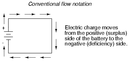
However, because we tend to associate the word “positive” with “surplus” and “negative” with “deficiency,” the standard label for electron charge does seem backward. Because of this, many engineers decided to retain the old concept of electricity with “positive” referring to a surplus of charge, and label charge flow (current) accordingly. This became known as conventional flow notation:

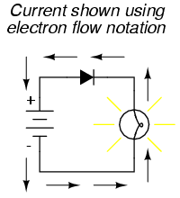
Others chose to designate charge flow according to the actual motion of electrons in a circuit. This form of symbology became known as electron flow notation:

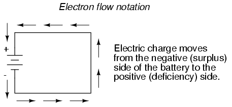
In conventional flow notation, we show the motion of charge according to the (technically incorrect) labels of + and -. This way the labels make sense, but the direction of charge flow is incorrect. In electron flow notation, we follow the actual motion of electrons in the circuit, but the + and - labels seem backward. Does it matter, really, how we designate charge flow in a circuit? Not really, so long as we’re consistent in the use of our symbols. You may follow an imagined direction of current (conventional flow) or the actual (electron flow) with equal success insofar as circuit analysis is concerned. Concepts of voltage, current, resistance, continuity, and even mathematical treatments such as Ohm’s Law (chapter 2) and Kirchhoff’s Laws (chapter 6) remain just as valid with either style of notation.

You will find conventional flow notation followed by most electrical engineers, and illustrated in most engineering textbooks. Electron flow is most often seen in introductory textbooks (this one included) and in the writings of professional scientists, especially solid-state physicists who are concerned with the actual motion of electrons in substances. These preferences are cultural, in the sense that certain groups of people have found it advantageous to envision electric current motion in certain ways. Being that most analyses of electric circuits do not depend on a technically accurate depiction of charge flow, the choice between conventional flow notation and electron flow notation is arbitrary . . . almost.

Many electrical devices tolerate real currents of either direction with no difference in operation. Incandescent lamps (the type utilizing a thin metal filament that glows white-hot with sufficient current), for example, produce light with equal efficiency regardless of current direction. They even function well on alternating current (AC), where the direction changes rapidly over time. Conductors and switches operate irrespective of current direction, as well. The technical term for this irrelevance of charge flow is nonpolarization. We could say then, that incandescent lamps, switches, and wires are nonpolarized components. Conversely, any device that functions differently on currents of different direction would be called a polarized device.

There are many such polarized devices used in electric circuits. Most of them are made of so-called semiconductor substances, and as such aren’t examined in detail until the third volume of this book series. Like switches, lamps, and batteries, each of these devices is represented in a schematic diagram by a unique symbol. As one might guess, polarized device symbols typically contain an arrow within them, somewhere, to designate a preferred or exclusive direction of current. This is where the competing notations of conventional and electron flow really matter. Because engineers from long ago have settled on conventional flow as their “culture’s” standard notation, and because engineers are the same people who invent electrical devices and the symbols representing them, the arrows used in these devices’ symbols all point in the direction of conventional flow, not electron flow. That is to say, all of these devices’ symbols have arrow marks that point against the actual flow of electrons through them.

Perhaps the best example of a polarized device is the diode. A diode is a one-way “valve” for electric current, analogous to a check valve for those familiar with plumbing and hydraulic systems. Ideally, a diode provides unimpeded flow for current in one direction (little or no resistance), but prevents flow in the other direction (infinite resistance). Its schematic symbol looks like this:

Placed within a battery/lamp circuit, its operation is as such:

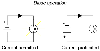
When the diode is facing in the proper direction to permit current, the lamp glows. Otherwise, the diode blocks all electron flow just like a break in the circuit, and the lamp will not glow.

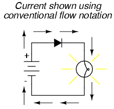
If we label the circuit current using conventional flow notation, the arrow symbol of the diode makes perfect sense: the triangular arrowhead points in the direction of charge flow, from positive to negative:

On the other hand, if we use electron flow notation to show the true direction of electron travel around the circuit, the diode’s arrow symbology seems backward:

For this reason alone, many people choose to make conventional flow their notation of choice when drawing the direction of charge motion in a circuit. If for no other reason, the symbols associated with semiconductor components like diodes make more sense this way. However, others choose to show the true direction of electron travel so as to avoid having to tell themselves, “just remember the electrons are actually moving the other way” whenever the true direction of electron motion becomes an issue.

In this series of textbooks, I have committed to using electron flow notation. Ironically, this was not my first choice. I found it much easier when I was first learning electronics to use conventional flow notation, primarily because of the directions of semiconductor device symbol arrows. Later, when I began my first formal training in electronics, my instructor insisted on using electron flow notation in his lectures. In fact, he asked that we take our textbooks (which were illustrated using conventional flow notation) and use our pens to change the directions of all the current arrows so as to point the “correct” way! His preference was not arbitrary, though. In his 20-year career as a U.S. Navy electronics technician, he worked on a lot of vacuum-tube equipment. Before the advent of semiconductor components like transistors, devices known as vacuum tubes or electron tubes were used to amplify small electrical signals. These devices work on the phenomenon of electrons hurtling through a vacuum, their rate of flow controlled by voltages applied between metal plates and grids placed within their path, and are best understood when visualized using electron flow notation.

When I graduated from that training program, I went back to my old habit of conventional flow notation, primarily for the sake of minimizing confusion with component symbols, since vacuum tubes are all but obsolete except in special applications. Collecting notes for the writing of this book, I had full intention of illustrating it using conventional flow.

Years later, when I became a teacher of electronics, the curriculum for the program I was going to teach had already been established around the notation of electron flow. Oddly enough, this was due in part to the legacy of my first electronics instructor (the 20-year Navy veteran), but that’s another story entirely! Not wanting to confuse students by teaching “differently” from the other instructors, I had to overcome my habit and get used to visualizing electron flow instead of conventional. Because I wanted my book to be a useful resource for my students, I begrudgingly changed plans and illustrated it with all the arrows pointing the “correct” way. Oh well, sometimes you just can’t win!

On a positive note (no pun intended), I have subsequently discovered that some students prefer electron flow notation when first learning about the behavior of semiconductive substances. Also, the habit of visualizing electrons flowing against the arrows of polarized device symbols isn’t that difficult to learn, and in the end I’ve found that I can follow the operation of a circuit equally well using either mode of notation. Still, I sometimes wonder if it would all be much easier if we went back to the source of the confusion—Ben Franklin’s errant conjecture—and fixed the problem there, calling electrons “positive” and protons “negative.”

Voltage and Current in a Practical Circuit

Because it takes energy to force electrons to flow against the opposition of a resistance, there will be voltage manifested (or “dropped”) between any points in a circuit with resistance between them. It is important to note that although the amount of current (the quantity of electrons moving past a given point every second) is uniform in a simple circuit, the amount of voltage (potential energy per unit charge) between different sets of points in a single circuit may vary considerably:

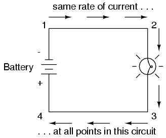
Take this circuit as an example. If we label four points in this circuit with the numbers 1, 2, 3, and 4, we will find that the amount of current conducted through the wire between points 1 and 2 is exactly the same as the amount of current conducted through the lamp (between points 2 and 3). This same quantity of current passes through the wire between points 3 and 4, and through the battery (between points 1 and 4).

However, we will find the voltage appearing between any two of these points to be directly proportional to the resistance within the conductive path between those two points, given that the amount of current along any part of the circuit’s path is the same (which, for this simple circuit, it is). In a normal lamp circuit, the resistance of a lamp will be much greater than the resistance of the connecting wires, so we should expect to see a substantial amount of voltage between points 2 and 3, with very little between points 1 and 2, or between 3 and 4. The voltage between points 1 and 4, of course, will be the full amount of “force” offered by the battery, which will be only slightly greater than the voltage across the lamp (between points 2 and 3).

This, again, is analogous to the water reservoir system:

Between points 2 and 3, where the falling water is releasing energy at the water-wheel, there is a difference of pressure between the two points, reflecting the opposition to the flow of water through the water-wheel. From point 1 to point 2, or from point 3 to point 4, where water is flowing freely through reservoirs with little opposition, there is little or no difference of pressure (no potential energy). However, the rate of water flow in this continuous system is the same everywhere (assuming the water levels in both pond and reservoir are unchanging): through the pump, through the water-wheel, and through all the pipes. So it is with simple electric circuits: the rate of electron flow is the same at every point in the circuit, although voltages may differ between different sets of points.

XXX . ___ . 000 . 222 Motion of a Charged Particle in a Magnetic Field

Electric and magnetic forces both affect the trajectory of charged particles, but in qualitatively different ways.

LEARNING OBJECTIVES

Compare the effects of the electric and the magnetic fields on the charged particle

KEY TAKEAWAYS

Key Points

The force on a charged particle due to an electric field is directed parallel to the electric field vector in the case of a positive charge, and anti-parallel in the case of a negative charge. It does not depend on the velocity of the particle.
In contrast, the magnetic force on a charge particle is orthogonal to the magnetic field vector, and depends on the velocity of the particle. The right hand rule can be used to determine the direction of the force.
An electric field may do work on a charged particle, while a magnetic field does no work.
The Lorentz force is the combination of the electric and magnetic force, which are often considered together for practical applications.
Electric field lines are generated on positive charges and terminate on negative ones. The field lines of an isolated charge are directly radially outward. The electric field is tangent to these lines.
Magnetic field lines, in the case of a magnet, are generated at the north pole and terminate on a south pole. Magnetic poles do not exist in isolation. Like in the case of electric field lines, the magnetic field is tangent to the field lines. Charged particles will spiral around these field lines.

Key Terms

orthogonal: Of two objects, at right angles; perpendicular to each other.

Electric vs. Magnetic Forces

Force due to both electric and magnetic forces will influence the motion of charged particles. However, the resulting change to the trajectory of the particles will differ qualitatively between the two forces. Below we will quickly review the two types of force and compare and contrast their effects on a charged particle.

Electrostatic Force and Magnetic Force on a Charged Particle

Recall that in a static, unchanging electric field E the force on a particle with charge q will be:

F = qE

Where F is the force vector, q is the charge, and E is the electric field vector. Note that the direction of F is identical to E in the case of a positivist charge q, and in the opposite direction in the case of a negatively charged particle. This electric field may be established by a larger charge, Q, acting on the smaller charge q over a distance r so that:

E = | \frac{F}{q} | = k | \frac{qQ}{{qr}^{2}} | = k \frac{| Q |}{r^{2}}

It should be emphasized that the electric force F acts parallel to the electric field E. The curl of the electric force is zero, i.e.:

▽ \times E = 0

A consequence of this is that the electric field may do work and a charge in a pure electric field will follow the tangent of an electric field line.

In contrast, recall that the magnetic force on a charged particle is orthogonal to the magnetic field such that:

F = qv \times B = qvBsin θ

where B is the magnetic field vector, v is the velocity of the particle and θ is the angle between the magnetic field and the particle velocity. The direction of F can be easily determined by the use of the right hand rule.

Right Hand Rule: Magnetic fields exert forces on moving charges. This force is one of the most basic known. The direction of the magnetic force on a moving charge is perpendicular to the plane formed by v and B and follows right hand rule–1 (RHR-1) as shown. The magnitude of the force is proportional to q, v, B, and the sine of the angle between v and B.

If the particle velocity happens to be aligned parallel to the magnetic field, or is zero, the magnetic force will be zero. This differs from the case of an electric field, where the particle velocity has no bearing, on any given instant, on the magnitude or direction of the electric force.

The angle dependence of the magnetic field also causes charged particles to move perpendicular to the magnetic field lines in a circular or helical fashion, while a particle in an electric field will move in a straight line along an electric field line.

A further difference between magnetic and electric forces is that magnetic fields do not net work, since the particle motion is circular and therefore ends up in the same place. We express this mathematically as:

W = \oint B \cdot dr = 0

Lorentz Force

The Lorentz force is the combined force on a charged particle due both electric and magnetic fields, which are often considered together for practical applications. If a particle of charge q moves with velocity v in the presence of an electric field E and a magnetic field B, then it will experience a force:

F = q [E + vBsin θ]

Electric and Magnetic Field Lines

We mentioned briefly above that the motion of charged particles relative to the field lines differs depending on whether one is dealing with electric or magnetic fields. There are some notable differences between how electric and magnetic field lines are conceptualized. The electric field lines from a positive isolated charge are simply a sequence of evenly-spaced, radially directed lines pointed outwards from the charge. In the case of a negative charge, the direction of the field is reversed. The electric field is directed tangent to the field lines. Of course, we imagine the field lines are more densely packed the larger the charges are. One can see clearly that the curl of the electric force is zero.

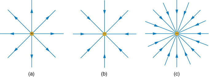
Electric Field Generated by Point Charges: The electric field surrounding three different point charges: (a) A positive charge; (b) a negative charge of equal magnitude; (c) a larger negative charge.

If multiple charges are involved, field lines are generated on positive charges, and terminate on negative ones.

In the case of magnets, field lines are generated on the north pole (+) and terminate on the south pole (-) – see the below figure. Magnetic ‘charges’, however, always come in pairs – there are no magnetic monopoles (isolated north or south poles). The curl of a magnetic field generated by a conventional magnet is therefore always non zero. Charged particles will spiral around these field lines, as long as the particles have some non-zero component of velocity directed perpendicular to the field lines.

Magnetic Pole Model: The magnetic pole model: two opposing poles, North (+) and South (−), separated by a distance d produce an H-field (lines).

A magnetic field may also be generated by a current with the field lines envisioned as concentric circles around the current-carrying wire.The magnetic force at any point in this case can be determined with the right hand rule, and will be perpendicular to both the current and the magnetic field.

Constant Velocity Produces a Straight-Line

If a charged particle’s velocity is parallel to the magnetic field, there is no net force and the particle moves in a straight line.

LEARNING OBJECTIVES

Identify conditions required for the particle to move in a straight line in the magnetic field

KEY TAKEAWAYS

Key Points

Newton’s first law of motion states that if an object experiences no net force, then its velocity is constant.
A particle with constant velocity will move along a straight line through space.
If a charged particle’s velocity is completely parallel to the magnetic field, the magnetic field will exert no force on the particle and thus the velocity will remain constant.
In the case that the velocity vector is neither parallel nor perpendicular to the magnetic field, the component of the velocity parallel to the field will remain constant.

Key Terms

straight-line motion: motion that proceeds in a single direction

Constant Velocity Produces Straight-Line Motion

Recall Newton’s first law of motion. If an object experiences no net force, then its velocity is constant: the object is either at rest (if its velocity is zero), or it moves in a straight line with constant speed (if its velocity is nonzero).

There are many cases where a particle may experience no net force. The particle could exist in a vacuum far away from any massive bodies (that exert gravitational forces) and electromagnetic fields. Or there could be two or more forces on the particle that are balanced such that the net force is zero. This is the case for, say, a particle suspended in an electric field with the electric force exactly counterbalancing gravity.

If the net force on a particle is zero, then the acceleration is necessarily zero from Newton’s second law: F=ma. If the acceleration is zero, any velocity the particle has will be maintained indefinitely (or until such time as the net force is no longer zero). Because velocity is a vector, the direction remains unchanged along with the speed, so the particle continues in a single direction, such as with a straight line.

Charged Particles Moving Parallel to Magnetic Fields

The force a charged particle “feels” due to a magnetic field is dependent on the angle between the velocity vector and the magnetic field vector B . Recall that the magnetic force is:

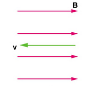
Zero Force When Velocity is Parallel to Magnetic Field: In the case above the magnetic force is zero because the velocity is parallel to the magnetic field lines.

F = qvBsin θ

If the magnetic field and the velocity are parallel (or antiparallel), then sinθ equals zero and there is no force. In this case a charged particle can continue with straight-line motion even in a strong magnetic field. If is between 0 and 90 degrees, then the component of v parallel to B remains unchanged.

Circular Motion

Since the magnetic force is always perpendicular to the velocity of a charged particle, the particle will undergo circular motion.

LEARNING OBJECTIVES

Describe conditions that lead to the circular motion of a charged particle in the magnetic field

KEY TAKEAWAYS

Key Points

The magnetic field does no work, so the kinetic energy and speed of a charged particle in a magnetic field remain constant.
The magnetic force, acting perpendicular to the velocity of the particle, will cause circular motion.
The centripetal force of the particle is provided by magnetic Lorentzian force so that $qvB = \frac{{mv}^{2}}{r}$ .
Solving for r above yields the gryoradius, or the radius of curvature of the path of a particle with charge q and mass m moving in a magnetic field of strength B. The gryoradius is then given by $r = \frac{mv}{qB}$ .
The cyclotron frequency (or, equivalently, gyrofrequency) is the number of cycles a particle completes around its circular circuit every second and is given by $f = \frac{qB}{2 π m}$ .

Key Terms

gyroradius: The radius of the circular motion of a charged particle in the presence of a uniform magnetic field.
cyclotron frequency: The frequency of a charged particle moving perpendicular to the direction of a uniform magnetic field B (constant magnitude and direction). Given by the equality of the centripetal force and magnetic Lorentz force.

Circular Motion of a Charged particle in a Magnetic Field

Magnetic forces can cause charged particles to move in circular or spiral paths. Particle accelerators keep protons following circular paths with magnetic force. Cosmic rays will follow spiral paths when encountering the magnetic field of astrophysical objects or planets (one example being Earth’s magnetic field). The bubble chamber photograph in the figure below shows charged particles moving in such curved paths. The curved paths of charged particles in magnetic fields are the basis of a number of phenomena and can even be used analytically, such as in a mass spectrometer. shows the path traced by particles in a bubble chamber.

Bubble Chamber: Trails of bubbles are produced by high-energy charged particles moving through the superheated liquid hydrogen in this artist’s rendition of a bubble chamber. There is a strong magnetic field perpendicular to the page that causes the curved paths of the particles. The radius of the path can be used to find the mass, charge, and energy of the particle.

So, does the magnetic force cause circular motion? Magnetic force is always perpendicular to velocity, so that it does no work on the charged particle. The particle’s kinetic energy and speed thus remain constant. The direction of motion is affected, but not the speed. This is typical of uniform circular motion. The simplest case occurs when a charged particle moves perpendicular to a uniform B-field, such as shown in. (If this takes place in a vacuum, the magnetic field is the dominant factor determining the motion. ) Here, the magnetic force (Lorentz force) supplies the centripetal force

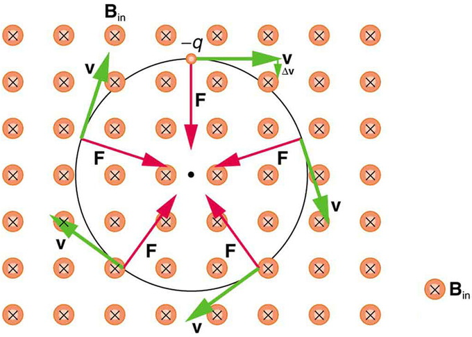
Circular Motion of Charged Particle in Magnetic Field: A negatively charged particle moves in the plane of the page in a region where the magnetic field is perpendicular into the page (represented by the small circles with x’s—like the tails of arrows). The magnetic force is perpendicular to the velocity, and so velocity changes in direction but not magnitude. Uniform circular motion results.

F_{c} = \frac{{mv}^{2}}{r}

Noting that

sin θ = 1

we see that

F = qvB .

The Lorentz magnetic force supplies the centripetal force, so these terms are equal:

qvB = \frac{{mv}^{2}}{r}

solving for r yields

r = \frac{mv}{qB}

Here, r, called the gyroradius or cyclotron radius, is the radius of curvature of the path of a charged particle with mass m and charge q, moving at a speed v perpendicular to a magnetic field of strength B. In other words, it is the radius of the circular motion of a charged particle in the presence of a uniform magnetic field. If the velocity is not perpendicular to the magnetic field, then v is the component of the velocity perpendicular to the field. The component of the velocity parallel to the field is unaffected, since the magnetic force is zero for motion parallel to the field. We’ll explore the consequences of this case in a later section on spiral motion.

A particle experiencing circular motion due to a uniform magnetic field is termed to be in a cyclotron resonance. The term comes from the name of a cyclic particle accelerator called a cyclotron, showed in. The cyclotron frequency (or, equivalently, gyrofrequency) is the number of cycles a particle completes around its circular circuit every second and can be found by solving for v above and substituting in the circulation frequency so that

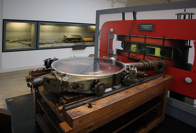
Cyclotron: A French cyclotron, produced in Zurich, Switzerland in 1937

f = \frac{v}{2 π r}

becomes

f = \frac{qB}{2 π m}

The cyclotron frequency is trivially given in radians per second by

ω = \frac{qB}{m}

Helical Motion

Helical motion results when the velocity vector is not perpendicular to the magnetic field vector.

LEARNING OBJECTIVES

Describe conditions that lead to the helical motion of a charged particle in the magnetic field

KEY TAKEAWAYS

Key Points

Previously, we have seen that circular motion results when the velocity of a charged particle is perpendicular to the magnetic field. The speed and kinetic energy of the particle remain constant, but the direction is altered at each instant by the perpendicular magnetic force.
If the velocity is not perpendicular to the magnetic field, we consider only the component of v that is perpendicular to the field when making our calculations.
The component of the velocity parallel to the field is unaffected, since the magnetic force is zero for motion parallel to the field. This produces helical motion.
Charges may spiral along field lines. If the strength of the magnetic field increases in the direction of motion, the field will exert a force to slow the charges and even reverse their direction. This is known as a magnetic mirror.

Key Terms

helical motion: The motion that is produced when one component of the velocity is constant in magnitude and direction (i.e., straight-line motion) while the other component is constant in speed but uniformly varies in direction (i.e., circular motion). It is the superposition of straight-line and circular motion.
magnetic mirror: A magnetic field configuration where the field strength changes when moving along a field line. The mirror effect results in a tendency for charged particles to bounce back from the high field region.

Helical Motion

In the section on circular motion we described the motion of a charged particle with the magnetic field vector aligned perpendicular to the velocity of the particle. In this case, the magnetic force is also perpendicular to the velocity (and the magnetic field vector, of course) at any given moment resulting in circular motion. The speed and kinetic energy of the particle remain constant, but the direction is altered at each instant by the perpendicular magnetic force. quickly reviews this situation in the case of a negatively charged particle in a magnetic field directed into the page.

What if the velocity is not perpendicular to the magnetic field? Then we consider only the component of v that is perpendicular to the field when making our calculations, so that the equations of motion become:

F_{c} = \frac{{mv}_{⊥}^{2}}{r}

F = qvBsin θ = {qv}_{⊥} B

The component of the velocity parallel to the field is unaffected, since the magnetic force is zero for motion parallel to the field. This produces helical motion (i.e., spiral motion) rather than a circular motion.

shows how electrons not moving perpendicular to magnetic field lines follow the field lines. The component of velocity parallel to the lines is unaffected, and so the charges spiral along the field lines. If field strength increases in the direction of motion, the field will exert a force to slow the charges (and even reverse their direction), forming a kind of magnetic mirror.

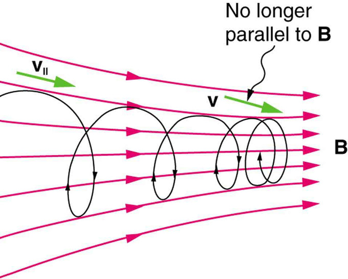
Helical Motion and Magnetic Mirrors: When a charged particle moves along a magnetic field line into a region where the field becomes stronger, the particle experiences a force that reduces the component of velocity parallel to the field. This force slows the motion along the field line and here reverses it, forming a “magnetic mirror. “

The motion of charged particles in magnetic fields are related to such different things as the Aurora Borealis or Aurora Australis (northern and southern lights) and particle accelerators. Charged particles approaching magnetic field lines may get trapped in spiral orbits about the lines rather than crossing them, as seen above. Some cosmic rays, for example, follow the Earth’s magnetic field lines, entering the atmosphere near the magnetic poles and causing the southern or northern lights through their ionization of molecules in the atmosphere. Those particles that approach middle latitudes must cross magnetic field lines, and many are prevented from penetrating the atmosphere. Cosmic rays are a component of background radiation; consequently, they give a higher radiation dose at the poles than at the equator.

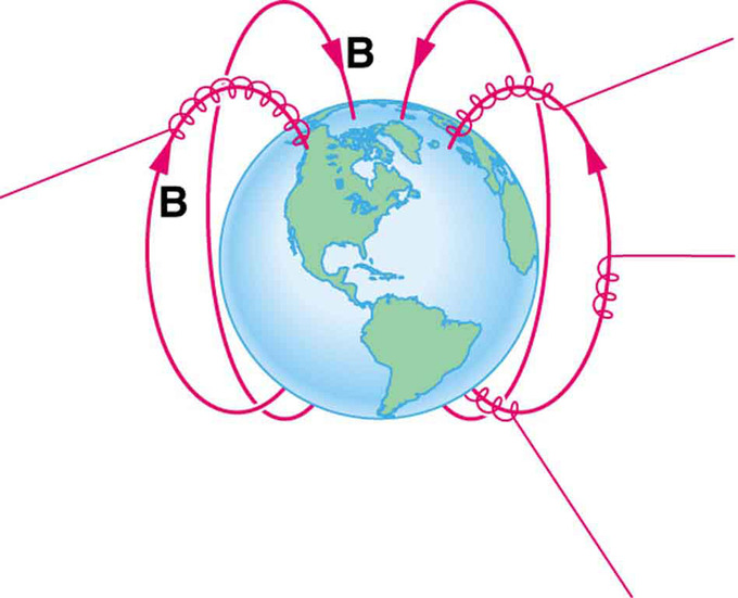
Charged Particles Spiral Along Earth’s Magnetic Field Lines: Energetic electrons and protons, components of cosmic rays, from the Sun and deep outer space often follow the Earth’s magnetic field lines rather than cross them. (Recall that the Earth’s north magnetic pole is really a south pole in terms of a bar magnet. )

Examples and Applications

Cyclotrons, magnetrons, and mass spectrometers represent practical technological applications of electromagnetic fields.

LEARNING OBJECTIVES

Discuss application of mass spectrometers, movement of charged particles in a cyclotron, and how microwaves are generated in the cavity magnetron

KEY TAKEAWAYS

Key Points

A cyclotron is a type of particle accelerator in which charged particles accelerate outwards from the center along a spiral path. The particles are held to a spiral trajectory by a static magnetic field and accelerated by a rapidly varying electric field.
The cavity magnetron is a high-powered vacuum tube that generates microwaves using the interaction of a stream of electrons with a magnetic field. The magnetron has applications in radar, heating, and lighting.
Mass spectrometers measure the mass-to-charge ratio of charged particles through the use of electromagnetic fields to segregate particles with different masses and/or charges. It can be used to determine the elemental composition of a molecule or sample.

Key Terms

cyclotron: An early particle accelerator in which charged particles were generated at a central source and accelerated spirally outward through a fixed magnetic and alternating electric fields.
mass spectrometer: A device used in mass spectrometry to discover the mass composition of a given substance.
magnetron: A device in which electrons are made to resonate in a specially shaped chamber and thus produce microwave radiation; used in radar, and in microwave ovens.

Examples and Applications – Motion of a Charged Particle in a Magnetic Field

Overview

Recall that the charged particles in a magnetic field will follow a circular or spiral path depending on the alignment of their velocity vector with the magnetic field vector. The consequences of such motion can have profoundly practical applications. Many technologies are based on the motion of charged particles in electromagnetic fields. We will explore some of these, including the cyclotron and synchrotron, cavity magnetron, and mass spectrometer.

Cyclotrons and Synchrotrons

A cyclotron is a type of particle accelerator in which charged particles accelerate outwards from the center along a spiral path. The particles are held to a spiral trajectory by a static magnetic field and accelerated by a rapidly varying (radio frequency ) electric field.

Cyclotron Sketch: Sketch of a particle being accelerated in a cyclotron, and being ejected through a beamline.

Cyclotrons accelerate charged particle beams using a high frequency alternating voltage which is applied between two “D”-shaped electrodes (also called “dees”). An additional static magnetic field is applied in perpendicular direction to the electrode plane, enabling particles to re-encounter the accelerating voltage many times at the same phase. To achieve this, the voltage frequency must match the particle’s cyclotron resonance frequency,

f = \frac{qB}{2 π m}

with the relativistic mass m and its charge q. This frequency is given by equality of centripetal force and magnetic Lorentz force. The particles, injected near the center of the magnetic field, increase their kinetic energy only when recirculating through the gap between the electrodes; thus they travel outwards along a spiral path. Their radius will increase until the particles hit a target at the perimeter of the vacuum chamber, or leave the cyclotron using a beam tube, enabling their use. The particles accelerated by the cyclotron can be used in particle therapy to treat some types of cancer. Additionally, cyclotrons are a good source of high-energy beams for nuclear physics experiments.

A synchrotron is an improvement upon the cyclotron in which the guiding magnetic field (bending the particles into a closed path) is time-dependent, being synchronized to a particle beam of increasing kinetic energy. The synchrotron is one of the first accelerator concepts that enable the construction of large-scale facilities, since bending, beam focusing and acceleration can be separated into different components.

Cavity Magnetron

The cavity magnetron is a high-powered vacuum tube that generates microwaves using the interaction of a stream of electrons with a magnetic field. All cavity magnetrons consist of a hot cathode with a high (continuous or pulsed) negative potential created by a high-voltage, direct-current power supply. The cathode is built into the center of an evacuated, lobed, circular chamber. A magnetic field parallel to the filament is imposed by a permanent magnet. The magnetic field causes the electrons, attracted to the (relatively) positive outer part of the chamber, to spiral outward in a circular path, a consequence of the Lorentz force. Spaced around the rim of the chamber are cylindrical cavities. The cavities are open along their length and connect the common cavity space. As electrons sweep past these openings, they induce a resonant, high-frequency radio field in the cavity, which in turn causes the electrons to bunch into groups.

Cavity Magnetron Diagram: A cross-sectional diagram of a resonant cavity magnetron. Magnetic lines of force are parallel to the geometric axis of this structure.

The sizes of the cavities determine the resonant frequency, and thereby the frequency of emitted microwaves. The magnetron is a self-oscillating device requiring no external elements other than a power supply. The magnetron has practical applications in radar, heating (as the primary component of a microwave oven), and lighting.

Mass Spectrometry

Mass spectrometry is an analytical technique that measures the mass-to-charge ratio of charged particles. It is used for determining masses of particles and determining the elemental composition of a sample or molecule.

Mass analyzers separate the ions according to their mass-to-charge ratio. The following two laws govern the dynamics of charged particles in electric and magnetic fields in a vacuum:

F = Q (E + v \times B)

(Lorentz force)

F = ma

Equating the above expressions for the force applied to the ion yields:

(m / Q) a = E + v \times B

This differential equation along with initial conditions completely determines the motion of a charged particle in terms of m/Q. There are many types of mass analyzers, using either static or dynamic fields, and magnetic or electric fields, but all operate according to the above differential equation.

The following figure illustrates one type of mass spectrometer. The deflections of the particles are dependent on the mass-to-charge ratio. In the case of isotopic carbon dioxide, each molecule has the same charge, but different masses. The mass spectrometer will segregate the particles spatially allowing a detector to measure the mass-to-charge ratio of each particle. Since the charge is known, the absolute mass can be determined trivially. The relative abundances can be inferred from counting the number of particles of each given mass.

Mass Spectrometry: Schematics of a simple mass spectrometer with sector type mass analyzer. This one is for the measurement of carbon dioxide isotope ratios (IRMS) as in the carbon-13 urea breath test.

The circuit is analogous to the wheel of a car driven over a corrugated road, as seen in. The regularly spaced bumps in the road are analogous to the voltage source, driving the wheel up and down. The shock absorber is analogous to the resistance damping and limiting the amplitude of the oscillation. Energy within the system goes back and forth between kinetic (analogous to maximum current, and energy stored in an inductor) and potential energy stored in the car spring (analogous to no current, and energy stored in the electric field of a capacitor). The amplitude of the wheels’ motion is a maximum if the bumps in the road are hit at the resonant frequency.

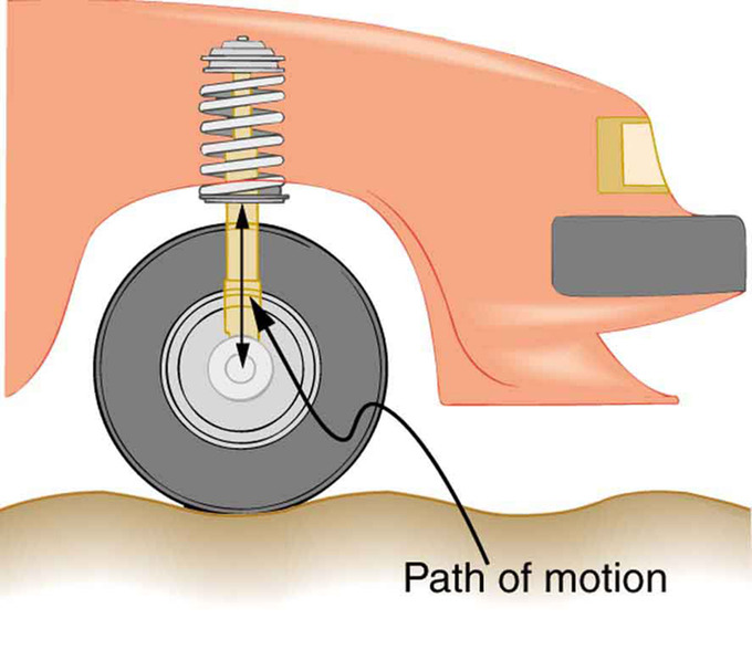
Forced Damped Motion of a Wheel on a Car Spring: The forced but damped motion of the wheel on the car spring is analogous to an RLC series AC circuit. The shock absorber damps the motion and dissipates energy, analogous to the resistance in an RLC circuit. The mass and spring determine the resonant frequency.

Broadest & DPPrecision Motion Technologies

Linear, Rotary, Piezo, Air Bearing, Servo, Stepper, Voice Coil, Linear Motor, Screw Drives, Parallel Kinematics

Why Ptechnologies. From traditional stepper motors to air bearing gantries; from piezo components to advanced ceramic hybrid drives and multi-axis piezo nanopositioning systems; from stacked (linear+rotary) positioners to 6-axis Hexapod parallel motion and alignment systems.

Talk to our enginee they will guide you to the most appropriate technology to solve your motion problem.

Select PI Products

Nanopositioning Stages and Ultra-Precision Positioning Systems


These stages are capable of providing nanometer size steps. PI offers different concepts for different applications, from the ultra-precise and fast piezo flexure stages for small travel ranges to large air bearing stages and exotic maglev systems.


Piezo Flexure Stages <1mm Travel, Sub-nm resolution	Air Bearing Stages Long Travel Best Straightness	Linear Motor Stages Mechanical Bearings	Hybrid Stages Piezo and Servo Motor	Magnetic Levitation Multi-Axis, Ultra Precision

Piezo Stages & Positioners: Flexure Direct Drives, Piezo Motor Long Travel Designs


PI offers several piezo-based positioning concepts. Flexure-guided stages provide the highest precision and speed, but are limited to typically <1 mm travel range. Several piezo motor concepts are offered for long travel ranges. Ultrasonic piezo motors provide higher speed, PiezoWalk motors excel in force generation, and stick-slip motors are very compact and cost effective.


Single Axis Flexure Stages Speed and Precision	XY and XYZ Flexure With Large Apertures	Tip/Tilt (Mirrors) High Speed	PIFOC Nano-Focus High Speed	Long Travel Piezo Motors Very compact, low cost

Hexapod 6-Axis Positioners and Motion Platforms (Stewart Platforms)


Hexapod parallel positioners provide extremely versatile multi-axis motion in all degrees of freedom. They are based on a 6-axis (XYZ, Pitch, Roll, Yaw) actuator system, arranged in parallel between a top and bottom platform. PI Hexapod positioners and motion simulators have many advantages over conventional multi-axis stages, such as improved dynamics, smaller package size and higher stiffness.


Miniature/Dynamics	High Dynamics	Medium Size	High-Load Hexapods	Extreme Conditions

Precision Air Bearing Stages, Components, Systems


Air bearings provide frictonless motion with excellent guiding precision (flatness/straightness) over long travel ranges, and with high load capacity. PI's air bearing stage designs are based on more than 200 man years of experience.


Rotary Stages	XY Stages	Linear Stages	Machining	Non-Motorized

Miniature Positioners: Stepper, Servo, Voice-Coil, Piezo Motor-Driven


Because one drive principle does not fit all applications, PI provides a number of different miniature stage concepts. From classical stepper and servo motors to high-speed linear motors and a variety of self-locking piezo motors with emphasis on precision, dynamics, cost and force generation.


Motorized Stepper, and Servo Motor	High Speed Ultrasonic Piezo Motor	Sub-Miniature Low Cost Inertia Motor	Flexure guided Fast & Precise, up to 1.8mm Travel	Linear Motor High Speed, Long Travel

Motorized Linear and Rotary Positioners and Actuators


Motorized positioning stages and actuators are based on mechanical bearings, stepper motor, servo motor or linear motor drives. Position encoders are used for feedback. PI offers a large selection of motor controllers.


Rotary Stages	XY/XYZ Stages	Vertical Stages	Linear Stages	Actuators

Precision Rotary Stages


The PI group has extensive knowledge in the design and manufacture of highly precise rotation stages and positioning systems. Customers use our rotary stages in a variety of applications such as beamline instrumentation, fiber-optical alignment, semiconductor inspection, bio-medical instrumentation and X-ray crystallography.


Air Bearing	Tip/Tilt & Gonio	Classical	Piezo Motor	Compact

Automation Actuators / Precision Actuators


PI currently offers a variety of automation and high precision actuators based on several drive technologies. Voice coil linear motors provide high speed long travel and long service life. Piezo flexure actuators can move in microseconds to milliseconds with ranges to 1 mm. Ultrasonic piezo high-speed motors cover ranges to 150 mm and acceleration to 10 g, based on a self-locking, non-magnetic drive principle. Serve and stepper lead and ballscrew actuators cover many traditional applications and piezo ratchet drives replace conventional manual micrometers.


Fast Voice Coil	Servo & Stepper	Piezo / Flexure	Piezo Ultrasonic	Piezo-Ratchet

Piezo Actuators, Stacks, Tubes, Benders: Direct Motion, Short Travel, Ultra-Fast


PI designs and manufactures all of its piezo actuators from the ground up. Piezo materials are manufactured at PI's Ceramic division. PI's PICMA multilayer stacks have been life tested by NASA/JPL for 100 billion cycles. Stacks and benders are available in both cofired multilayer (low voltage) and classical, glued designs.


Piezo Stacks & Chips	Preloaded Actuators	Tubes & Tubular Stacks	Bimorph Benders	Amplified / Guided Actuators

Piezo Motors: Long Travel, Ultrasonic, Stick-Slip, PiezoWalk Drives


Piezo motors provide several advantages over conventional motors: smaller, lower energy consumption, self-locking at rest, high force compared to size, intrinsically vacuum-compatible and non-magnetic, very fast response down to the microsecond range.


PiezoMike Screw Drives Piezo Ratchet	Stick-Slip Linear Motors Mini Rod Drive	PiezoWalk Motors High Force & Precision	Ultrasonic Motor Stages High Speed	Stick-Slip Mini Positioner High Resolution

Ultra-Precision Positioners for Microscopy


Super-resolution microscopy and electron microscopy depends on high precision motion systems with nanometer resolution, fast response, and extreme position stability. PI offers a number of solutions with flexure based piezo drives, self-locking ultrasonic motor stages, and fast nano-focus drives in both standard and vacuum versions. Controllers are compatible with all major image acquisition packages.


PIFOC NanoFocus Drives	Z-Scanners for Slides and K-Plates	PInano XY and XYZ scanners	Ultra-Precision Piezo Stages	High Stabilty Long Travel Stages

Active Optics / Fast Tip-Tilt Piezo Steering Mirrors


PI offers piezo and voice-coil-based tip/tilt stages and steering mirrors, from miniature standard units to large custom designs for astronomy and aerospace. For fastest response and highest resolution, they make use of frictionless flexure guides and high-speed solid-state piezo drives or linear magnetic motors.


Single-Axis Platforms / Shifters	Multi-Axis Tip/Tilt Platform	Z/Tip/Tilt Platforms (w/Aperture)	Large Angle Tip/Tilt Mirrors	Steering Mirrors for Astronomy

Photonics Alignment, Automated Fiber Positioners


Fiber alignment / photonics test automation systems come in different flavors from compact XYZ motorized fiber positioners to fully automated 6 degree of freedom hexapod alignment systems with controller and software. Integrated closed-loop piezo scanners provide extremely fast response for the shortest possible alignment times.


H-206 Automated 6-Axis Alignment Systems	Miniature Hexapod Alignment Systems	High-Speed XYZ Automatic Alignment	Free Space Optical Comm	"Add-on" Piezo High Speed XYZ

Piezo Drivers and Controllers


Closed-loop piezo positioning and motion controllers are the key to high performance piezo motion. PI provides a very large spectrum, from miniature OEM modules, to compact digital-servo bench top controllers and high-end multi-axis controllers with advanced servo algorithms specifically developed for solid-state piezo ceramic drives.


Digital Servo	Reference Class	OEM Modules	High-Power	Modular Analog

Stepper and Servo Motor Controllers


These controllers are optimized for PI’s motorized positioning stages. Models for magnetic DC-servo, micro-stepped motors as well as for several kinds of ceramic linear and rotary motors are available. Hexapod controllers handle all coordinate transformation and path planning. User friendly software, drivers, and examples are included.


Single Channel Servo & Stepper	Multi-Axis Servo	Multi-Purpose Microstep + Servo	Hexapod 6-Axis Controllers	Piezo Motor Controllers



Vacuum Positioners / Systems	Value-Added Piezo Assemblies	Nano-Positioning Sensors


Linear Rotary	Custom OEM Assemblies Advanced PZT Materials	Capacitance Sensors Electronics

Jumat, 11 Mei 2018

Magnetic bearing

Design

Back to Flash Basics

Future advances

Active magnetic bearing

Maintenance-Free bearing for maximum speeds

Magnetic bearing motors / generatorsComplete drive solutions for high-speed applications

Magnetic bearing spindlesComplete solutions for challenging processing tasks

Dynamic ceramics

Life

Other bearing materials

In the wind

The birth of a ceramic ball

Life

Other bearing materials

In the wind

The birth of a ceramic ball

Atoms and Electrons

Figure 1-1. Hydrogen and copper atoms

Electric Charge and Current

Figure 1-2. Electrons moving in a wire

Figure 1-3. Modeling electrons with marbles in a tube

Current Flow in a Basic Circuit

Figure 1-4. A simple DC circuit

Ohm’s Law

Power

Resistance

Figure 1-5. Circuit resistance example

Figure 1-6. A typical resistor

Example: Building a Voltage Divider

Figure 1-7. A simple voltage divider

Summary

Conventional Versus Electron Flow

LEARNING OBJECTIVES

KEY TAKEAWAYS

Key Points

Key Terms

Electric vs. Magnetic Forces

Electrostatic Force and Magnetic Force on a Charged Particle

Lorentz Force

Electric and Magnetic Field Lines

Constant Velocity Produces a Straight-Line

LEARNING OBJECTIVES

KEY TAKEAWAYS

Key Points

Key Terms

Constant Velocity Produces Straight-Line Motion

Charged Particles Moving Parallel to Magnetic Fields

Circular Motion

LEARNING OBJECTIVES

KEY TAKEAWAYS

Key Points

Key Terms

Circular Motion of a Charged particle in a Magnetic Field

Helical Motion

LEARNING OBJECTIVES

KEY TAKEAWAYS

Key Points

Key Terms

Helical Motion

Examples and Applications

LEARNING OBJECTIVES

KEY TAKEAWAYS

Key Points

Key Terms

Examples and Applications – Motion of a Charged Particle in a Magnetic Field

Overview

Cyclotrons and Synchrotrons

Cavity Magnetron

Mass Spectrometry

Broadest & DPPrecision Motion Technologies

Linear, Rotary, Piezo, Air Bearing, Servo, Stepper, Voice Coil, Linear Motor, Screw Drives, Parallel Kinematics

Nanopositioning Stages and Ultra-Precision Positioning Systems

Piezo Stages & Positioners: Flexure Direct Drives, Piezo Motor Long Travel Designs

Hexapod 6-Axis Positioners and Motion Platforms (Stewart Platforms)

Precision Air Bearing Stages, Components, Systems

Miniature Positioners: Stepper, Servo, Voice-Coil, Piezo Motor-Driven

Motorized Linear and Rotary Positioners and Actuators

Precision Rotary Stages