


x ample : Pickling is the first step in the production process of cold-rolled strip. First, the coils from the hot strip mill are welded into endless strips. In the continuous pickling line the scale that forms on the hot strip during hot rolling is rinsed with hydrochloric acid. This creates a bare metallic strip surface.
To ensure an uninterrupted pickling process, the continuous pickling line features a strip accumulator, also called a looper. The strip is accumulated to avoid unintentional standstill or operational stops, for coil welding.


X . I
Kinds of Sensors
Sensors are tools that can be used to detect something (such as: temperature, speed, distance etc.) and often serve to measure the magnitude (amount) of something. The sensor is a type of transducer (converting power into another power) such as changing mechanical, magnetic, heat, chemical and light variations into voltage and electric current. Sensors are usually categorized by the meter and play an important role in the control of modern manufacturing processes. The sensors provide the eye, ears, nose and tongue of the tongue and become the microprocessor's brain of industrial automation systems. So the sensor is very important in the manufacture of automation tools such as in the field of industry, and others.
x ample sensor function picture :
Here are the various Sensors and their Functions and Implementation:
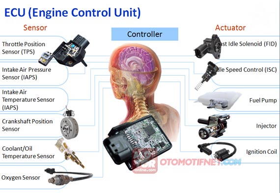
Sensors On Electronic Fuel Injection
1. Light sensorLight Sensor

Light sensors, as the name suggests, are used against objects that have shapes of color or light, which are converted into different power.The light sensor consists of 3 kinds of categories:· Photovoltaic, the working procedure of this sensor that is, convert direct light energy into electrical energy, in the presence of irradiation of light will cause the movement of electrons and generate voltage.· Photoconductive this sensor provides a change of resistance (resistance) in the cells. Principle of work, the higher the intensity of light received the sensor, the smaller the value of the resistance.· Photoelectric, work-principle sensor based on reflection due to change of position / distance of a light source (infrared or laser) or its reflecting target, consisting of the light source and receiver pair.Here are some examples of light sensors:
A. LDR (Light Dependent Resistor)This sensor serves to convert the intensity of light into electrical resistance. The working principle of LDR (Light Dependent Resistors) is, the higher the intensity of light that concerns the surface of LDR (Light Dependent Resistor), the greater the electrical resistance generated, and vice versa. This sensor can be implemented in the manufacture of automatic lights. Lights that automatically live at night, and die during the day. Lights live because the light intensity read by the sensor is very minimal, and vice versa.
B. PhotodiodeThis photodiode serves to change the intensity of light into diode conductivity. A photodiode similar to the diode in general, the difference in this photodiode is the fitting of a lens focusing lens to focus the falling beam at the "p n" encounter.
B. PhotodiodeThis photodiode serves to change the intensity of light into diode conductivity. A photodiode similar to the diode in general, the difference in this photodiode is the fitting of a lens focusing lens to focus the falling beam at the "p n" encounter.
Working principle: The light emitting energy falling at the "p n" encounter causes an electron to move to a higher energy level. The electrons move out of the band's valence leaving the hole generating a free electron pair and a hole. know about this one robot, Line Follower or more details Line Tracer. The Photodiode sensor is used to accept the color difference input from the line object reflected by the LED light beam, so that Line Tracer can proceed precisely over the line.
C. Phototransistor

Serves to change the intensity of light into the conductivity of the transistor. The phototransistor is similar to the transistor in general. The difference lies in, phototransistor mounted a lens focusing lens on the base foot to focus the falling light at meeting "p n".
2. Pressure Sensor
Pressure SensorThis sensor pressure sensor has a transducer that measures wire strain, which converts mechanical voltage into electrical signals. The basis of its sensing on changes in transducer resistance (transducer) is changed due to changes in length and area of its cross section. Examples of products that use Pressure sensors, such as: A tool for automatic detection of adult blood pressure. The device is performed with a cuff attached to the patient's arm, then pumped up to a certain pressure which is then just done a blood pressure measurement.
3. Proximity Sensor
Proximity SensorThe proximity sensor or so-called "proximity sensor" is a sensor capable of detecting the presence of nearby objects without direct physical contact. Usually this sensor consists of a solid-state electronics instrument wrapped tightly to protect from the effects of vibration, fluid, chemicals, and corrosive excessive. Proximity sensors can be applied to sensing conditions on objects that are considered too small or soft to drive a mechanical switch. Example of utilization of Proximity sensor is on Smartphone which in its application using Air Gesture technique. Where users can do access management to the smartphone without making physical contact to the smartphone screen.

4. Ultrasonic Sensor
Ultrasonic Sensor
Ultrasonic sensors work on the principle of the reflection of sound waves, where these sensors produce sound waves which then capture them back with time difference as the basis for their sensing. The time difference between the sound waves emitted by the re-capture of the sound waves is directly proportional to the distance or height of the object that reflects it. Types of objects that can be sensed include: solid objects, liquid, granules and textiles. Many products are on processing using Ultrasonic sensors.
5. Speed Sensor (RPM)
Speed Sensor (RPM)The process of sensing the speed sensor is the reverse process of a motor, in which a rotating axis on a generator will produce a voltage proportional to the speed of the rotation of the object. Rotation speed is often measured using sensors that sense magnetic pulses (induces) that arise when a magnetic field occurs. For example on speedometer. The tool measures the speed of motor speed in kilometers per hour.
6. Magnet Sensor
Magnet Sensor
Magnet sensor or also called magnetic relay, is a tool that will be affected by magnetic field and will give change condition at output. Like a switch two conditions (on / off) is driven by the presence of magnetic field around it. Usually this sensor is packaged in a vacuum packing and free of dust, moisture, smoke or steam. Implementation of this tool such as, Computer-based magnetic field measurements consist of magnetic field sensor UGN3503, Op-Amp LM358 and ADC 0804. The working principle of the tool is closer to the magnet on the sensor. The sensor output of the voltage will be amplified by the op-amp to be processed by the ADC. Next the voltage is converted by ADC into digital data, then processed by computer with visual basic program and the result is displayed on PC.
7. Sensor Encoder (Encoder)
Encoding Sensor
Encoding Sensor

Encoder (Encoder) is used to convert linear or spin movements into digital signals, where the rotating sensor monitors the rotary motion of a device. This sensor usually consists of 2 layers of encoding type, namely; First, an additional rotary encoder (which transmits a certain amount of pulses for each round) that will generate a square wave on the object being rotated. Second, the absolute coding (which completes certain binary codes for each corner position) has the same way of working with the exceptions, the more or more density of the resulting square wave pulse in order to form an encoding in a particular arrangement. Examples of implementation of this sensor can be made into a system that can calculate the strength of earthquakes by using incremental rotary encoder sensor and processed by microcontroller...
8. Temperature SensorTemperature Sensor
As the name suggests, this sensor is certainly used to detect the temperature. There are 4 main types of commonly used temperature sensors, namely thermocouple (T / C) resistance temperature detector (RTD), thermistor and IC sensor. The thermocouple is essentially composed of a pair of hot and cold transducers which are connected together and melted together, in which there is a distinction arising between the joint and the reference line acting as a reference. Resistance Temperature Detector (RTD) has a basic principle in electrical resistance of metals that vary in proportion to temperature. The comparison of these variations is precision with a high degree of consistency / stability on detection of detainees. Platinum is a material that is often used because it has temperature resistance, linier , stability and reproducibility. Thermistors are heat-sensitive resistors that usually have a negative temperature coefficient, because when the temperature increases the resistance decreases or vice versa. This type is very sensitive with a 5% resistance per C so it can detect small temperature changes. While the IC Sensor is a temperature sensor with integrated circuit that uses chip silicon for weakness sensing . It has a very linear output voltage and current configuration. Usually this sensor is mostly installed on the smoke detector tool used to track the fire.
9. Flow Meter Sensor
Sensor Flow MeterFlow Meter is a sensor used to determine the flow of a material both solid and liquid. In the Industrial World there are various types of Sensor Flow this. For Yang Liquid usually use Turbine type, Electromagnetic, venture meter and others. As for Solid material is usually used from a combination of some instrument equipment used as Flow Meter, for example Weigh Feeder .
10. Flame sensor
Flame Sensor
This flame sensor can detect a flame with a wavelength of 760 nm ~ 1100 nm. In many robot matches, the detection of flame becomes one of the common rules of the race that never lags. Therefore this sensor is very useful, which you can make 'eye' for the robot to be able to detect the source of the flame, or looking for the ball. Suitable for use on fire-fighting robot and soccer robot.
This flame sensor has a reading angle of 60 degrees, and operates at a temperature of 25 -85 degrees Celsius. And of course for your attention, that the distance between the sensor and the detected object should not be too close, to avoid sensor damage.

X . II
Sensors and Transducers

But in order for an electronic circuit or system to perform any useful task or function it needs to be able to communicate with the “real world” whether this is by reading an input signal from an “ON/OFF” switch or by activating some form of output device to illuminate a single light.
In other words, an Electronic System or circuit must be able to “do” something and Sensors and Transducers are the perfect components for doing this.
Related Products: Ambient Light Sensor | Temperature and Humidity Sensors
The word “Transducer” is the collective term used for both Sensors which can be used to sense a wide range of different energy forms such as movement, electrical signals, radiant energy, thermal or magnetic energy etc , and Actuators which can be used to switch voltages or currents.
There are many different types of sensors and transducers, both analogue and digital and input and output available to choose from. The type of input or output transducer being used, really depends upon the type of signal or process being “Sensed” or “Controlled” but we can define a sensor and transducers as devices that converts one physical quantity into another.
Devices which perform an “Input” function are commonly called Sensors because they “sense” a physical change in some characteristic that changes in response to some excitation, for example heat or force and covert that into an electrical signal. Devices which perform an “Output” function are generally called Actuators and are used to control some external device, for example movement or sound.
Electrical Transducers are used to convert energy of one kind into energy of another kind, so for example, a microphone (input device) converts sound waves into electrical signals for the amplifier to amplify (a process), and a loudspeaker (output device) converts these electrical signals back into sound waves and an example of this type of simple Input / Output (I/O) system is given below.
 There are many different types of sensors and transducers available in the marketplace, and the choice of which one to use really depends upon the quantity being measured or controlled, with the more common types given in the table below.
Input type transducers or sensors, produce a voltage or signal output response which is proportional to the change in the quantity that they are measuring (the stimulus). The type or amount of the output signal depends upon the type of sensor being used. But generally, all types of sensors can be classed as two kinds, either Passive Sensors or Active Sensors.
Generally, active sensors require an external power supply to operate, called an excitation signal which is used by the sensor to produce the output signal. Active sensors are self-generating devices because their own properties change in response to an external effect producing for example, an output voltage of 1 to 10v DC or an output current such as 4 to 20mA DC. Active sensors can also produce signal amplification.
A good example of an active sensor is an LVDT sensor or a strain gauge. Strain gauges are pressure-sensitive resistive bridge networks that are external biased (excitation signal) in such a way as to produce an output voltage in proportion to the amount of force and/or strain being applied to the sensor.
Unlike an active sensor, a passive sensor does not need any additional power source or excitation voltage. Instead a passive sensor generates an output signal in response to some external stimulus. For example, a thermocouple which generates its own voltage output when exposed to heat. Then passive sensors are direct sensors which change their physical properties, such as resistance, capacitance or inductance etc.
But as well as analogue sensors, Digital Sensors produce a discrete output representing a binary number or digit such as a logic level “0” or a logic level “1”.

 Analogue sensors tend to produce output signals that are changing smoothly and continuously over time. These signals tend to be very small in value from a few mico-volts (uV) to several milli-volts (mV), so some form of amplification is required.
Then circuits which measure analogue signals usually have a slow response and/or low accuracy. Also analogue signals can be easily converted into digital type signals for use in micro-controller systems by the use of analogue-to-digital converters, or ADC’s.
In our simple example above, the speed of the rotating shaft is measured by using a digital LED/Opto-detector sensor. The disc which is fixed to a rotating shaft (for example, from a motor or robot wheels), has a number of transparent slots within its design. As the disc rotates with the speed of the shaft, each slot passes by the sensor in turn producing an output pulse representing a logic “1” or logic “0” level.
These pulses are sent to a register of counter and finally to an output display to show the speed or revolutions of the shaft. By increasing the number of slots or “windows” within the disc more output pulses can be produced for each revolution of the shaft. The advantage of this is that a greater resolution and accuracy is achieved as fractions of a revolution can be detected. Then this type of sensor arrangement could also be used for positional control with one of the discs slots representing a reference position.
Compared to analogue signals, digital signals or quantities have very high accuracies and can be both measured and “sampled” at a very high clock speed. The accuracy of the digital signal is proportional to the number of bits used to represent the measured quantity. For example, using a processor of 8 bits, will produce an accuracy of 0.390% (1 part in 256). While using a processor of 16 bits gives an accuracy of 0.0015%, (1 part in 65,536) or 260 times more accurate. This accuracy can be maintained as digital quantities are manipulated and processed very rapidly, millions of times faster than analogue signals.
In most cases, sensors and more specifically analogue sensors generally require an external power supply and some form of additional amplification or filtering of the signal in order to produce a suitable electrical signal which is capable of being measured or used. One very good way of achieving both amplification and filtering within a single circuit is to use Operational Amplifiers as seen before.
The very small analogue signal voltages produced by a sensor such as a few milli-volts or even pico-volts can be amplified many times over by a simple op-amp circuit to produce a much larger voltage signal of say 5v or 5mA that can then be used as an input signal to a microprocessor or analogue-to-digital based system.
Therefore, to provide any useful signal a sensors output signal has to be amplified with an amplifier that has a voltage gain up to 10,000 and a current gain up to 1,000,000 with the amplification of the signal being linear with the output signal being an exact reproduction of the input, just changed in amplitude.
Then amplification is part of signal conditioning. So when using analogue sensors, generally some form of amplification (Gain), impedance matching, isolation between the input and output or perhaps filtering (frequency selection) may be required before the signal can be used and this is conveniently performed by Operational Amplifiers.
Also, when measuring very small physical changes the output signal of a sensor can become “contaminated” with unwanted signals or voltages that prevent the actual signal required from being measured correctly. These unwanted signals are called “Noise“. This Noise or Interference can be either greatly reduced or even eliminated by using signal conditioning or filtering techniques as we discussed in the Active Filter tutorial.
By using either a Low Pass, or a High Pass or even Band Pass filter the “bandwidth” of the noise can be reduced to leave just the output signal required. For example, many types of inputs from switches, keyboards or manual controls are not capable of changing state rapidly and so low-pass filter can be used. When the interference is at a particular frequency, for example mains frequency, narrow band reject or Notch filters can be used to produce frequency selective filters.
 Were some random noise still remains after filtering it may be necessary to take several samples and then average them to give the final value so increasing the signal-to-noise ratio. Either way, both amplification and filtering play an important role in interfacing both sensors and transducers to microprocessor and electronics based systems in “real world” conditions.
In the next tutorial about Sensors, we will look at Positional Sensors which measure the position and/or displacement of physical objects meaning the movement from one position to another for a specific distance or angle.
In other words, an Electronic System or circuit must be able to “do” something and Sensors and Transducers are the perfect components for doing this.
Related Products: Ambient Light Sensor | Temperature and Humidity Sensors
The word “Transducer” is the collective term used for both Sensors which can be used to sense a wide range of different energy forms such as movement, electrical signals, radiant energy, thermal or magnetic energy etc , and Actuators which can be used to switch voltages or currents.
There are many different types of sensors and transducers, both analogue and digital and input and output available to choose from. The type of input or output transducer being used, really depends upon the type of signal or process being “Sensed” or “Controlled” but we can define a sensor and transducers as devices that converts one physical quantity into another.
Devices which perform an “Input” function are commonly called Sensors because they “sense” a physical change in some characteristic that changes in response to some excitation, for example heat or force and covert that into an electrical signal. Devices which perform an “Output” function are generally called Actuators and are used to control some external device, for example movement or sound.
Electrical Transducers are used to convert energy of one kind into energy of another kind, so for example, a microphone (input device) converts sound waves into electrical signals for the amplifier to amplify (a process), and a loudspeaker (output device) converts these electrical signals back into sound waves and an example of this type of simple Input / Output (I/O) system is given below.
Simple Input / Output System using Sound Transducers
Common Sensors and Transducers
| Quantity being Measured | Input Device (Sensor) | Output Device (Actuator) |
| Light Level | Light Dependant Resistor (LDR) Photodiode Photo-transistor Solar Cell | Lights & Lamps LED’s & Displays Fibre Optics |
| Temperature | Thermocouple Thermistor Thermostat Resistive Temperature Detectors | Heater Fan |
| Force/Pressure | Strain Gauge Pressure Switch Load Cells | Lifts & Jacks Electromagnet Vibration |
| Position | Potentiometer Encoders Reflective/Slotted Opto-switch LVDT | Motor Solenoid Panel Meters |
| Speed | Tacho-generator Reflective/Slotted Opto-coupler Doppler Effect Sensors | AC and DC Motors Stepper Motor Brake |
| Sound | Carbon Microphone Piezo-electric Crystal | Bell Buzzer Loudspeaker |
Generally, active sensors require an external power supply to operate, called an excitation signal which is used by the sensor to produce the output signal. Active sensors are self-generating devices because their own properties change in response to an external effect producing for example, an output voltage of 1 to 10v DC or an output current such as 4 to 20mA DC. Active sensors can also produce signal amplification.
A good example of an active sensor is an LVDT sensor or a strain gauge. Strain gauges are pressure-sensitive resistive bridge networks that are external biased (excitation signal) in such a way as to produce an output voltage in proportion to the amount of force and/or strain being applied to the sensor.
Unlike an active sensor, a passive sensor does not need any additional power source or excitation voltage. Instead a passive sensor generates an output signal in response to some external stimulus. For example, a thermocouple which generates its own voltage output when exposed to heat. Then passive sensors are direct sensors which change their physical properties, such as resistance, capacitance or inductance etc.
But as well as analogue sensors, Digital Sensors produce a discrete output representing a binary number or digit such as a logic level “0” or a logic level “1”.
Analogue and Digital Sensors
Analogue Sensors
Analogue Sensors produce a continuous output signal or voltage which is generally proportional to the quantity being measured. Physical quantities such as Temperature, Speed, Pressure, Displacement, Strain etc are all analogue quantities as they tend to be continuous in nature. For example, the temperature of a liquid can be measured using a thermometer or thermocouple which continuously responds to temperature changes as the liquid is heated up or cooled down.Thermocouple used to produce an Analogue Signal
Then circuits which measure analogue signals usually have a slow response and/or low accuracy. Also analogue signals can be easily converted into digital type signals for use in micro-controller systems by the use of analogue-to-digital converters, or ADC’s.
Digital Sensors
As its name implies, Digital Sensors produce a discrete digital output signals or voltages that are a digital representation of the quantity being measured. Digital sensors produce a Binary output signal in the form of a logic “1” or a logic “0”, (“ON” or “OFF”). This means then that a digital signal only produces discrete (non-continuous) values which may be outputted as a single “bit”, (serial transmission) or by combining the bits to produce a single “byte” output (parallel transmission).Light Sensor used to produce an Digital Signal
These pulses are sent to a register of counter and finally to an output display to show the speed or revolutions of the shaft. By increasing the number of slots or “windows” within the disc more output pulses can be produced for each revolution of the shaft. The advantage of this is that a greater resolution and accuracy is achieved as fractions of a revolution can be detected. Then this type of sensor arrangement could also be used for positional control with one of the discs slots representing a reference position.
Compared to analogue signals, digital signals or quantities have very high accuracies and can be both measured and “sampled” at a very high clock speed. The accuracy of the digital signal is proportional to the number of bits used to represent the measured quantity. For example, using a processor of 8 bits, will produce an accuracy of 0.390% (1 part in 256). While using a processor of 16 bits gives an accuracy of 0.0015%, (1 part in 65,536) or 260 times more accurate. This accuracy can be maintained as digital quantities are manipulated and processed very rapidly, millions of times faster than analogue signals.
In most cases, sensors and more specifically analogue sensors generally require an external power supply and some form of additional amplification or filtering of the signal in order to produce a suitable electrical signal which is capable of being measured or used. One very good way of achieving both amplification and filtering within a single circuit is to use Operational Amplifiers as seen before.
Signal Conditioning of Sensors
As we saw in the Operational Amplifier tutorial, op-amps can be used to provide amplification of signals when connected in either inverting or non-inverting configurations.The very small analogue signal voltages produced by a sensor such as a few milli-volts or even pico-volts can be amplified many times over by a simple op-amp circuit to produce a much larger voltage signal of say 5v or 5mA that can then be used as an input signal to a microprocessor or analogue-to-digital based system.
Therefore, to provide any useful signal a sensors output signal has to be amplified with an amplifier that has a voltage gain up to 10,000 and a current gain up to 1,000,000 with the amplification of the signal being linear with the output signal being an exact reproduction of the input, just changed in amplitude.
Then amplification is part of signal conditioning. So when using analogue sensors, generally some form of amplification (Gain), impedance matching, isolation between the input and output or perhaps filtering (frequency selection) may be required before the signal can be used and this is conveniently performed by Operational Amplifiers.
Also, when measuring very small physical changes the output signal of a sensor can become “contaminated” with unwanted signals or voltages that prevent the actual signal required from being measured correctly. These unwanted signals are called “Noise“. This Noise or Interference can be either greatly reduced or even eliminated by using signal conditioning or filtering techniques as we discussed in the Active Filter tutorial.
By using either a Low Pass, or a High Pass or even Band Pass filter the “bandwidth” of the noise can be reduced to leave just the output signal required. For example, many types of inputs from switches, keyboards or manual controls are not capable of changing state rapidly and so low-pass filter can be used. When the interference is at a particular frequency, for example mains frequency, narrow band reject or Notch filters can be used to produce frequency selective filters.
Typical Op-amp Filters
In the next tutorial about Sensors, we will look at Positional Sensors which measure the position and/or displacement of physical objects meaning the movement from one position to another for a specific distance or angle.
As their name implies, Position Sensors detect the position of something which means that they are referenced either to or from some fixed point or position. These types of sensors provide a “positional” feedback.
One method of determining a position, is to use either “distance”, which could be the distance between two points such as the distance travelled or moved away from some fixed point, or by “rotation” (angular movement). For example, the rotation of a robots wheel to determine its distance travelled along the ground. Either way, Position Sensors can detect the movement of an object in a straight line using Linear Sensors or by its angular movement using Rotational Sensors.

Potentiometer
Potentiometers come in a wide range of designs and sizes such as the commonly available round rotational type or the longer and flat linear slider types. When used as a position sensor the moveable object is connected directly to the rotational shaft or slider of the potentiometer.
A DC reference voltage is applied across the two outer fixed connections forming the resistive element. The output voltage signal is taken from the wiper terminal of the sliding contact as shown below.
This configuration produces a potential or voltage divider type circuit output which is proportional to the shaft position. Then for example, if you apply a voltage of say 10v across the resistive element of the potentiometer the maximum output voltage would be equal to the supply voltage at 10 volts, with the minimum output voltage equal to 0 volts. Then the potentiometer wiper will vary the output signal from 0 to 10 volts, with 5 volts indicating that the wiper or slider is at its half-way or center position.
 The output signal (Vout) from the potentiometer is taken from the centre wiper connection as it moves along the resistive track, and is proportional to the angular position of the shaft.
 While resistive potentiometer position sensors have many advantages: low cost, low tech, easy to use etc, as a position sensor they also have many disadvantages: wear due to moving parts, low accuracy, low repeatability, and limited frequency response.
But there is one main disadvantage of using the potentiometer as a positional sensor. The range of movement of its wiper or slider (and hence the output signal obtained) is limited to the physical size of the potentiometer being used.
For example a single turn rotational potentiometer generally only has a fixed mechanical rotation of between 0o and about 240 to 330o maximum. However, multi-turn pots of up to 3600o (10 x 360o) of mechanical rotation are also available.
Most types of potentiometers use carbon film for their resistive track, but these types are electrically noisy (the crackle on a radio volume control), and also have a short mechanical life.
Wire-wound pots also known as rheostats, in the form of either a straight wire or wound coil resistive wire can also be used, but wire wound pots suffer from resolution problems as their wiper jumps from one wire segment to the next producing a logarithmic (LOG) output resulting in errors in the output signal. These too suffer from electrical noise.
For high precision low noise applications conductive plastic resistance element type polymer film or cermet type potentiometers are now available. These pots have a smooth low friction electrically linear (LIN) resistive track giving them a low noise, long life and excellent resolution and are available as both multi-turn and single turn devices. Typical applications for this type of high accuracy position sensor is in computer game joysticks, steering wheels, industrial and robot applications.
It basically consists of three coils wound on a hollow tube former, one forming the primary coil and the other two coils forming identical secondaries connected electrically together in series but 180o out of phase either side of the primary coil.
A moveable soft iron ferromagnetic core (sometimes called an “armature”) which is connected to the object being measured, slides or moves up and down inside the tubular body of the LVDT.
A small AC reference voltage called the “excitation signal” (2 – 20V rms, 2 – 20kHz) is applied to the primary winding which in turn induces an EMF signal into the two adjacent secondary windings (transformer principles).
If the soft iron magnetic core armature is exactly in the centre of the tube and the windings, “null position”, the two induced emf’s in the two secondary windings cancel each other out as they are 180o out of phase, so the resultant output voltage is zero. As the core is displaced slightly to one side or the other from this null or zero position, the induced voltage in one of the secondaries will be become greater than that of the other secondary and an output will be produced.
The polarity of the output signal depends upon the direction and displacement of the moving core. The greater the movement of the soft iron core from its central null position the greater will be the resulting output signal. The result is a differential voltage output which varies linearly with the cores position. Therefore, the output signal from this type of position sensor has both an amplitude that is a linear function of the cores displacement and a polarity that indicates direction of movement.
The phase of the output signal can be compared to the primary coil excitation phase enabling suitable electronic circuits such as the AD592 LVDT Sensor Amplifier to know which half of the coil the magnetic core is in and thereby know the direction of travel.
 When the armature is moved from one end to the other through the centre position the output voltages changes from maximum to zero and back to maximum again but in the process changes its phase angle by 180 deg’s. This enables the LVDT to produce an output AC signal whose magnitude represents the amount of movement from the centre position and whose phase angle represents the direction of movement of the core.
A typical application of a linear variable differential transformer (LVDT) sensor would be as a pressure transducer, were the pressure being measured pushes against a diaphragm to produce a force. The force is then converted into a readable voltage signal by the sensor.
Advantages of the linear variable differential transformer, or LVDT compared to a resistive potentiometer are that its linearity, that is its voltage output to displacement is excellent, very good accuracy, good resolution, high sensitivity as well as frictionless operation. They are also sealed for use in hostile environments.
Proximity sensors, are non-contact position sensors that use a magnetic field for detection with the simplest magnetic sensor being the reed switch. In an inductive sensor, a coil is wound around an iron core within an electromagnetic field to form an inductive loop.
When a ferromagnetic material is placed within the eddy current field generated around the inductive sensor, such as a ferromagnetic metal plate or metal screw, the inductance of the coil changes significantly. The proximity sensors detection circuit detects this change producing an output voltage. Therefore, inductive proximity sensors operate under the electrical principle of Faraday’s Law of inductance.
 An inductive proximity sensor has four main components; The oscillator which produces the electromagnetic field, the coil which generates the magnetic field, the detection circuit which detects any change in the field when an object enters it and the output circuit which produces the output signal, either with normally closed (NC) or normally open (NO) contacts.
Inductive proximity sensors allow for the detection of metallic objects in front of the sensor head without any physical contact of the object itself being detected. This makes them ideal for use in dirty or wet environments. The “sensing” range of proximity sensors is very small, typically 0.1mm to 12mm.

Proximity Sensor
As well as industrial applications, inductive proximity sensors are also commonly used to control the flow of traffic by changing of traffic lights at junctions and cross roads. Rectangular inductive loops of wire are buried into the tarmac road surface.
When a car or other road vehicle passes over this inductive loop, the metallic body of the vehicle changes the loops inductance and activates the sensor thereby alerting the traffic lights controller that there is a vehicle waiting.
One main disadvantage of these types of position sensors is that they are “Omni-directional”, that is they will sense a metallic object either above, below or to the side of it. Also, they do not detect non-metallic objects although Capacitive Proximity Sensors and Ultrasonic Proximity Sensors are available. Other commonly available magnetic positional sensors include: reed switches, Hall Effect Sensors and variable reluctance sensors.
All optical encoders work on the same basic principle. Light from an LED or infra-red light source is passed through a rotating high-resolution encoded disk that contains the required code patterns, either binary, grey code or BCD. Photo detectors scan the disk as it rotates and an electronic circuit processes the information into a digital form as a stream of binary output pulses that are fed to counters or controllers which determine the actual angular position of the shaft.
There are two basic types of rotary optical encoders, Incremental Encoders and Absolute Position Encoders.

Encoder Disk
Incremental Encoders, also known as quadrature encoders or relative rotary encoder, are the simplest of the two position sensors. Their output is a series of square wave pulses generated by a photocell arrangement as the coded disk, with evenly spaced transparent and dark lines called segments on its surface, moves or rotates past the light source. The encoder produces a stream of square wave pulses which, when counted, indicates the angular position of the rotating shaft.
Incremental encoders have two separate outputs called “quadrature outputs”. These two outputs are displaced at 90o out of phase from each other with the direction of rotation of the shaft being determined from the output sequence.
The number of transparent and dark segments or slots on the disk determines the resolution of the device and increasing the number of lines in the pattern increases the resolution per degree of rotation. Typical encoded discs have a resolution of up to 256 pulses or 8-bits per rotation.
The simplest incremental encoder is called a tachometer. It has one single square wave output and is often used in unidirectional applications where basic position or speed information only is required. The “Quadrature” or “Sine wave” encoder is the more common and has two output square waves commonly called channel A and channel B. This device uses two photo detectors, slightly offset from each other by 90o thereby producing two separate sine and cosine output signals.
 By using the Arc Tangent mathematical function the angle of the shaft in radians can be calculated. Generally, the optical disk used in rotary position encoders is circular, then the resolution of the output will be given as: θ = 360/n, where n equals the number of segments on coded disk.
Then for example, the number of segments required to give an incremental encoder a resolution of 1o will be: 1o = 360/n, therefore, n = 360 windows, etc. Also the direction of rotation is determined by noting which channel produces an output first, either channel A or channel B giving two directions of rotation, A leads B or B leads A. This arrangement is shown below.
 One main disadvantage of incremental encoders when used as a position sensor, is that they require external counters to determine the absolute angle of the shaft within a given rotation. If the power is momentarily shut off, or if the encoder misses a pulse due to noise or a dirty disc, the resulting angular information will produce an error. One way of overcoming this disadvantage is to use absolute position encoders.
 One main advantage of an absolute encoder is its non-volatile memory which retains the exact position of the encoder without the need to return to a “home” position if the power fails. Most rotary encoders are defined as “single-turn” devices, but absolute multi-turn devices are available, which obtain feedback over several revolutions by adding extra code disks.
Typical application of absolute position encoders are in computer hard drives and CD/DVD drives were the absolute position of the drives read/write heads are monitored or in printers/plotters to accurately position the printing heads over the paper.
In this tutorial about Position Sensors, we have looked at several examples of sensors that can be used to measure the position or presence of objects. In the next tutorial we will look at sensors that are used to measure temperature such as thermistors, thermostats and thermocouples, and as such are known commonly as Temperature Sensors.
Temperature Sensors
These types of temperature sensor vary from simple ON/OFF thermostatic devices which control a domestic hot water heating system to highly sensitive semiconductor types that can control complex process control furnace plants.
We remember from our school science classes that the movement of molecules and atoms produces heat (kinetic energy) and the greater the movement, the more heat that is generated. Temperature Sensors measure the amount of heat energy or even coldness that is generated by an object or system, allowing us to “sense” or detect any physical change to that temperature producing either an analogue or digital output.
There are many different types of Temperature Sensor available and all have different characteristics depending upon their actual application. A temperature sensor consists of two basic physical types:
The bi-metallic strip can be used itself as an electrical switch or as a mechanical way of operating an electrical switch in thermostatic controls and are used extensively to control hot water heating elements in boilers, furnaces, hot water storage tanks as well as in vehicle radiator cooling systems.
 The thermostat consists of two thermally different metals stuck together back to back. When it is cold the contacts are closed and current passes through the thermostat. When it gets hot, one metal expands more than the other and the bonded bi-metallic strip bends up (or down) opening the contacts preventing the current from flowing.

On/Off Thermostat
There are two main types of bi-metallic strips based mainly upon their movement when subjected to temperature changes. There are the “snap-action” types that produce an instantaneous “ON/OFF” or “OFF/ON” type action on the electrical contacts at a set temperature point, and the slower “creep-action” types that gradually change their position as the temperature changes.
Snap-action type thermostats are commonly used in our homes for controlling the temperature set point of ovens, irons, immersion hot water tanks and they can also be found on walls to control the domestic heating system.
Creeper types generally consist of a bi-metallic coil or spiral that slowly unwinds or coils-up as the temperature changes. Generally, creeper type bi-metallic strips are more sensitive to temperature changes than the standard snap ON/OFF types as the strip is longer and thinner making them ideal for use in temperature gauges and dials etc.
Although very cheap and are available over a wide operating range, one main disadvantage of the standard snap-action type thermostats when used as a temperature sensor, is that they have a large hysteresis range from when the electrical contacts open until when they close again. For example, it may be set to 20oC but may not open until 22oC or close again until 18oC.
So the range of temperature swing can be quite high. Commercially available bi-metallic thermostats for home use do have temperature adjustment screws that allow for a more precise desired temperature set-point and hysteresis level to be pre-set.

Thermistor
Thermistors are generally made from ceramic materials such as oxides of nickel, manganese or cobalt coated in glass which makes them easily damaged. Their main advantage over snap-action types is their speed of response to any changes in temperature, accuracy and repeatability.
Most types of thermistor’s have a Negative Temperature Coefficient of resistance or (NTC), that is their resistance value goes DOWN with an increase in the temperature, and of course there are some which have a Positive Temperature Coefficient, (PTC), in that their resistance value goes UP with an increase in temperature.
Thermistors are constructed from a ceramic type semiconductor material using metal oxide technology such as manganese, cobalt and nickel, etc. The semiconductor material is generally formed into small pressed discs or balls which are hermetically sealed to give a relatively fast response to any changes in temperature.
Thermistors are rated by their resistive value at room temperature (usually at 25oC), their time constant (the time to react to the temperature change) and their power rating with respect to the current flowing through them. Like resistors, thermistors are available with resistance values at room temperature from 10’s of MΩ down to just a few Ohms, but for sensing purposes those types with values in the kilo-ohms are generally used.
Thermistors are passive resistive devices which means we need to pass a current through it to produce a measurable voltage output. Then thermistors are generally connected in series with a suitable biasing resistor to form a potential divider network and the choice of resistor gives a voltage output at some pre-determined temperature point or value for example:


 By changing the fixed resistor value of R2 (in our example 1kΩ) to a potentiometer or preset, a voltage output can be obtained at a predetermined temperature set point for example, 5v output at 60oC and by varying the potentiometer a particular output voltage level can be obtained over a wider temperature range.
It needs to be noted however, that thermistor’s are non-linear devices and their standard resistance values at room temperature is different between different thermistor’s, which is due mainly to the semiconductor materials they are made from. The Thermistor, have an exponential change with temperature and therefore have a Beta temperature constant ( β ) which can be used to calculate its resistance for any given temperature point.
However, when used with a series resistor such as in a voltage divider network or Whetstone Bridge type arrangement, the current obtained in response to a voltage applied to the divider/bridge network is linear with temperature. Then, the output voltage across the resistor becomes linear with temperature.

A Resistive RTD
Resistive temperature detectors have positive temperature coefficients (PTC) but unlike the thermistor their output is extremely linear producing very accurate measurements of temperature.
However, they have very poor thermal sensitivity, that is a change in temperature only produces a very small output change for example, 1Ω/oC.
The more common types of RTD’s are made from platinum and are called Platinum Resistance Thermometer or PRT‘s with the most commonly available of them all the Pt100 sensor, which has a standard resistance value of 100Ω at 0oC. The downside is that Platinum is expensive and one of the main disadvantages of this type of device is its cost.
Like the thermistor, RTD’s are passive resistive devices and by passing a constant current through the temperature sensor it is possible to obtain an output voltage that increases linearly with temperature. A typical RTD has a base resistance of about 100Ω at 0oC, increasing to about 140Ω at 100oC with an operating temperature range of between -200 to +600oC.
Because the RTD is a resistive device, we need to pass a current through them and monitor the resulting voltage. However, any variation in resistance due to self heat of the resistive wires as the current flows through it, I2R , (Ohms Law) causes an error in the readings. To avoid this, the RTD is usually connected into a Whetstone Bridge network which has additional connecting wires for lead-compensation and/or connection to a constant current source.
Thermocouples are thermoelectric sensors that basically consists of two junctions of dissimilar metals, such as copper and constantan that are welded or crimped together. One junction is kept at a constant temperature called the reference (Cold) junction, while the other the measuring (Hot) junction. When the two junctions are at different temperatures, a voltage is developed across the junction which is used to measure the temperature sensor as shown below.
 The operating principal of a thermocouple is very simple and basic. When fused together the junction of the two dissimilar metals such as copper and constantan produces a “thermo-electric” effect which gives a constant potential difference of only a few millivolts (mV) between them. The voltage difference between the two junctions is called the “Seebeck effect” as a temperature gradient is generated along the conducting wires producing an emf. Then the output voltage from a thermocouple is a function of the temperature changes.
If both the junctions are at the same temperature the potential difference across the two junctions is zero in other words, no voltage output as V1 = V2. However, when the junctions are connected within a circuit and are both at different temperatures a voltage output will be detected relative to the difference in temperature between the two junctions, V1 – V2. This difference in voltage will increase with temperature until the junctions peak voltage level is reached and this is determined by the characteristics of the two dissimilar metals used.
Thermocouples can be made from a variety of different materials enabling extreme temperatures of
between -200oC to over +2000oC to be measured. With such a large choice of materials and temperature range, internationally recognised standards have been developed complete with thermocouple colour codes to allow the user to choose the correct thermocouple sensor for a particular application. The British colour code for standard thermocouples is given below.
The three most common thermocouple materials used above for general temperature measurement are Iron-Constantan (Type J), Copper-Constantan (Type T), and Nickel-Chromium (Type K). The output voltage from a thermocouple is very small, only a few millivolts (mV) for a 10oC change in temperature difference and because of this small voltage output some form of amplification is generally required.
 The type of amplifier, either discrete or in the form of an Operational Amplifier needs to be carefully selected, because good drift stability is required to prevent recalibration of the thermocouple at frequent intervals. This makes the chopper and instrumentation type of amplifier preferable for most temperature sensing applications.
Other Temperature Sensor Types not mentioned here include, Semiconductor Junction Sensors, Infra-red and Thermal Radiation Sensors, Medical type Thermometers, Indicators and Colour Changing Inks or Dyes.
In this tutorial about “Temperature Sensor Types”, we have looked at several examples of sensors that can be used to measure changes in temperature. In the next tutorial we will look at sensors that are used to measure light quantity, such as Photodiodes, Phototransistors, Photovoltaic Cells and the Light Dependent Resistor.
The light sensor is a passive devices that convert this “light energy” whether visible or in the infra-red parts of the spectrum into an electrical signal output. Light sensors are more commonly known as “Photoelectric Devices” or “Photo Sensors” because the convert light energy (photons) into electricity (electrons).
Photoelectric devices can be grouped into two main categories, those which generate electricity when illuminated, such as Photo-voltaics or Photo-emissives etc, and those which change their electrical properties in some way such as Photo-resistors or Photo-conductors. This leads to the following classification of devices.
Photoresistors are Semiconductor devices that use light energy to control the flow of electrons, and hence the current flowing through them. The commonly used Photoconductive Cell is called the Light Dependent Resistor or LDR.

Typical LDR
As its name implies, the Light Dependent Resistor (LDR) is made from a piece of exposed semiconductor material such as cadmium sulphide that changes its electrical resistance from several thousand Ohms in the dark to only a few hundred Ohms when light falls upon it by creating hole-electron pairs in the material.
The net effect is an improvement in its conductivity with a decrease in resistance for an increase in illumination. Also, photoresistive cells have a long response time requiring many seconds to respond to a change in the light intensity.
Materials used as the semiconductor substrate include, lead sulphide (PbS), lead selenide (PbSe), indium antimonide (InSb) which detect light in the infra-red range with the most commonly used of all photoresistive light sensors being Cadmium Sulphide (Cds).
Cadmium sulphide is used in the manufacture of photoconductive cells because its spectral response curve closely matches that of the human eye and can even be controlled using a simple torch as a light source. Typically then, it has a peak sensitivity wavelength (λp) of about 560nm to 600nm in the visible spectral range.
 The most commonly used photoresistive light sensor is the ORP12 Cadmium Sulphide photoconductive cell. This light dependent resistor has a spectral response of about 610nm in the yellow to orange region of light. The resistance of the cell when unilluminated (dark resistance) is very high at about 10MΩ’s which falls to about 100Ω’s when fully illuminated (lit resistance).
To increase the dark resistance and therefore reduce the dark current, the resistive path forms a zigzag pattern across the ceramic substrate. The CdS photocell is a very low cost device often used in auto dimming, darkness or twilight detection for turning the street lights “ON” and “OFF”, and for photographic exposure meter type applications.
 Connecting a light dependant resistor in series with a standard resistor like this across a single DC supply voltage has one major advantage, a different voltage will appear at their junction for different levels of light.
The amount of voltage drop across series resistor, R2 is determined by the resistive value of the light dependant resistor, RLDR. This ability to generate different voltages produces a very handy circuit called a “Potential Divider” or Voltage Divider Network.
As we know, the current through a series circuit is common and as the LDR changes its resistive value due to the light intensity, the voltage present at VOUT will be determined by the voltage divider formula. An LDR’s resistance, RLDR can vary from about 100Ω’s in the sun light, to over 10MΩ’s in absolute darkness with this variation of resistance being converted into a voltage variation at VOUT as shown.
One simple use of a Light Dependent Resistor, is as a light sensitive switch as shown below.

LDR Switch
This basic light sensor circuit is of a relay output light activated switch. A potential divider circuit is formed between the photoresistor, LDR and the resistor R1. When no light is present ie in darkness, the resistance of the LDR is very high in the Megaohms (MΩ’s) range so zero base bias is applied to the transistor TR1 and the relay is de-energised or “OFF”.
As the light level increases the resistance of the LDR starts to decrease causing the base bias voltage at V1 to rise. At some point determined by the potential divider network formed with resistor R1, the base bias voltage is high enough to turn the transistor TR1 “ON” and thus activate the relay which in turn is used to control some external circuitry. As the light level falls back to darkness again the resistance of the LDR increases causing the base voltage of the transistor to decrease, turning the transistor and relay “OFF” at a fixed light level determined again by the potential divider network.
By replacing the fixed resistor R1 with a potentiometer VR1, the point at which the relay turns “ON” or “OFF” can be pre-set to a particular light level. This type of simple circuit shown above has a fairly low sensitivity and its switching point may not be consistent due to variations in either temperature or the supply voltage. A more sensitive precision light activated circuit can be easily made by incorporating the LDR into a “Wheatstone Bridge” arrangement and replacing the transistor with an Operational Amplifier as shown.
 In this basic dark sensing circuit, the light dependent resistor LDR1 and the potentiometer VR1 form one adjustable arm of a simple resistance bridge network, also known commonly as a Wheatstone bridge, while the two fixed resistors R1 and R2 form the other arm. Both sides of the bridge form potential divider networks across the supply voltage whose outputs V1 and V2 are connected to the non-inverting and inverting voltage inputs respectively of the operational amplifier.
The operational amplifier is configured as a Differential Amplifier also known as a voltage comparator with feedback whose output voltage condition is determined by the difference between the two input signals or voltages, V1 and V2. The resistor combination R1 and R2 form a fixed voltage reference at input V2, set by the ratio of the two resistors. The LDR – VR1 combination provides a variable voltage input V1 proportional to the light level being detected by the photoresistor.
As with the previous circuit the output from the operational amplifier is used to control a relay, which is protected by a free wheel diode, D1. When the light level sensed by the LDR and its output voltage falls below the reference voltage set at V2 the output from the op-amp changes state activating the relay and switching the connected load.
Likewise as the light level increases the output will switch back turning “OFF” the relay. The hysteresis of the two switching points is set by the feedback resistor Rf can be chosen to give any suitable voltage gain of the amplifier.
The operation of this type of light sensor circuit can also be reversed to switch the relay “ON” when the light level exceeds the reference voltage level and vice versa by reversing the positions of the light sensor LDR and the potentiometer VR1. The potentiometer can be used to “pre-set” the switching point of the differential amplifier to any particular light level making it ideal as a simple light sensor project circuit.

Photo-diode
The construction of the Photodiode light sensor is similar to that of a conventional PN-junction diode except that the diodes outer casing is either transparent or has a clear lens to focus the light onto the PN junction for increased sensitivity. The junction will respond to light particularly longer wavelengths such as red and infra-red rather than visible light.
This characteristic can be a problem for diodes with transparent or glass bead bodies such as the 1N4148 signal diode. LED’s can also be used as photodiodes as they can both emit and detect light from their junction. All PN-junctions are light sensitive and can be used in a photo-conductive unbiased voltage mode with the PN-junction of the photodiode always “Reverse Biased” so that only the diodes leakage or dark current can flow.
The current-voltage characteristic (I/V Curves) of a photodiode with no light on its junction (dark mode) is very similar to a normal signal or rectifying diode. When the photodiode is forward biased, there is an exponential increase in the current, the same as for a normal diode. When a reverse bias is applied, a small reverse saturation current appears which causes an increase of the depletion region, which is the sensitive part of the junction. Photodiodes can also be connected in a current mode using a fixed bias voltage across the junction. The current mode is very linear over a wide range.
 When used as a light sensor, a photodiodes dark current (0 lux) is about 10uA for geranium and 1uA for silicon type diodes. When light falls upon the junction more hole/electron pairs are formed and the leakage current increases. This leakage current increases as the illumination of the junction increases.
Thus, the photodiodes current is directly proportional to light intensity falling onto the PN-junction. One main advantage of photodiodes when used as light sensors is their fast response to changes in the light levels, but one disadvantage of this type of photodevice is the relatively small current flow even when fully lit.
The following circuit shows a photo-current-to-voltage converter circuit using an operational amplifier as the amplifying device. The output voltage (Vout) is given as Vout = Ip × Rf and which is proportional to the light intensity characteristics of the photodiode.
This type of circuit also utilizes the characteristics of an operational amplifier with two input terminals at about zero voltage to operate the photodiode without bias. This zero-bias op-amp configuration gives a high impedance loading to the photodiode resulting in less influence by dark current and a wider linear range of the photocurrent relative to the radiant light intensity. Capacitor Cf is used to prevent oscillation or gain peaking and to set the output bandwidth (1/2πRC).
 Photodiodes are very versatile light sensors that can turn its current flow both “ON” and “OFF” in nanoseconds and are commonly used in cameras, light meters, CD and DVD-ROM drives, TV remote controls, scanners, fax machines and copiers etc, and when integrated into operational amplifier circuits as infrared spectrum detectors for fibre optic communications, burglar alarm motion detection circuits and numerous imaging, laser scanning and positioning systems etc.

Photo-transistor
An alternative photo-junction device to the photodiode is the Phototransistor which is basically a photodiode with amplification. The Phototransistor light sensor has its collector-base PN-junction reverse biased exposing it to the radiant light source.
Phototransistors operate the same as the photodiode except that they can provide current gain and are much more sensitive than the photodiode with currents are 50 to 100 times greater than that of the standard photodiode and any normal transistor can be easily converted into a phototransistor light sensor by connecting a photodiode between the collector and base.
Phototransistors consist mainly of a bipolar NPN Transistor with its large base region electrically unconnected, although some phototransistors allow a base connection to control the sensitivity, and which uses photons of light to generate a base current which in turn causes a collector to emitter current to flow. Most phototransistors are NPN types whose outer casing is either transparent or has a clear lens to focus the light onto the base junction for increased sensitivity.
 In the NPN transistor the collector is biased positively with respect to the emitter so that the base/collector junction is reverse biased. therefore, with no light on the junction normal leakage or dark current flows which is very small. When light falls on the base more electron/hole pairs are formed in this region and the current produced by this action is amplified by the transistor.
Usually the sensitivity of a phototransistor is a function of the DC current gain of the transistor. Therefore, the overall sensitivity is a function of collector current and can be controlled by connecting a resistance between the base and the emitter but for very high sensitivity optocoupler type applications, Darlington phototransistors are generally used.

Photo-darlington
Photodarlington transistors use a second bipolar NPN transistor to provide additional amplification or when higher sensitivity of a photodetector is required due to low light levels or selective sensitivity, but its response is slower than that of an ordinary NPN phototransistor.
Photo darlington devices consist of a normal phototransistor whose emitter output is coupled to the base of a larger bipolar NPN transistor. Because a darlington transistor configuration gives a current gain equal to a product of the current gains of two individual transistors, a photodarlington device produces a very sensitive detector.
Typical applications of Phototransistors light sensors are in opto-isolators, slotted opto switches, light beam sensors, fibre optics and TV type remote controls, etc. Infrared filters are sometimes required when detecting visible light.
Another type of photojunction semiconductor light sensor worth a mention is the Photo-thyristor. This is a light activated thyristor or Silicon Controlled Rectifier, SCR that can be used as a light activated switch in AC applications. However their sensitivity is usually very low compared to equivalent photodiodes or phototransistors.
To help increase their sensitivity to light, photo-thyristors are made thinner around the gate junction. The downside to this process is that it limits the amount of anode current that they can switch. Then for higher current AC applications they are used as pilot devices in opto-couplers to switch larger more conventional thyristors.
However, unlike the other photo devices we have looked at above which use light intensity even from a torch to operate, photovoltaic solar cells work best using the suns radiant energy.
Solar cells are used in many different types of applications to offer an alternative power source from conventional batteries, such as in calculators, satellites and now in homes offering a form of renewable power.

Photovoltaic Cell
Photovoltaic cells are made from single crystal silicon PN junctions, the same as photodiodes with a very large light sensitive region but are used without the reverse bias. They have the same characteristics as a very large photodiode when in the dark.
When illuminated the light energy causes electrons to flow through the PN junction and an individual solar cell can generate an open circuit voltage of about 0.58v (580mV). Solar cells have a “Positive” and a “Negative” side just like a battery.
Individual solar cells can be connected together in series to form solar panels which increases the output voltage or connected together in parallel to increase the available current. Commercially available solar panels are rated in Watts, which is the product of the output voltage and current (Volts times Amps) when fully lit.
 The amount of available current from a solar cell depends upon the light intensity, the size of the cell and its efficiency which is generally very low at around 15 to 20%. To increase the overall efficiency of the cell commercially available solar cells use polycrystalline silicon or amorphous silicon, which have no crystalline structure, and can generate currents of between 20 to 40mA per cm2.
Other materials used in the construction of photovoltaic cells include Gallium Arsenide, Copper Indium Diselenide and Cadmium Telluride. These different materials each have a different spectrum band response, and so can be “tuned” to produce an output voltage at different wavelengths of light.
In this tutorial about Light Sensors, we have looked at several examples of devices that are classed as Light Sensors. This includes those with and those without PN-junctions that can be used to measure the intensity of light.
In the next tutorial we will look at output devices called Actuators. Actuators convert an electrical signal into a corresponding physical quantity such as movement, force, or sound. One such commonly used output device is the Electromagnetic Relay.
But there are also a variety of electrical and electronic devices which are classed as Output devices used to control or operate some external physical process. These output devices are commonly called Actuators.
Actuators convert an electrical signal into a corresponding physical quantity such as movement, force, sound etc. An actuator is also classed as a transducer because it changes one type of physical quantity into another and is usually activated or operated by a low voltage command signal. Actuators can be classed as either binary or continuous devices based upon the number of stable states their output has.
For example, a relay is a binary actuator as it has two stable states, either energised and latched or de-energised and unlatched, while a motor is a continuous actuator because it can rotate through a full 360o motion. The most common types of actuators or output devices are Electrical Relays, Lights, Motors and Loudspeakers.
We saw previously that solenoids can be used to electrically open latches, doors, open or close valves, and in a variety of robotic and mechatronic applications, etc. However, if the solenoid plunger is used to operate one or more sets of electrical contacts, we have a device called a relay that is so useful it can be used in an infinite number of different ways and in this tutorial we will look at Electrical Relays.
Electrical Relays can also be divided into mechanical action relays called “Electromechanical Relays” and those which use semiconductor transistors, thyristors, triacs, etc, as their switching device called “Solid State Relays” or SSR’s.

An Electrical Relay
The most fundamental control of any equipment is the ability to turn it “ON” and “OFF”. The easiest way to do this is using switches to interrupt the electrical supply. Although switches can be used to control something, they have their disadvantages. The biggest one is that they have to be manually (physically) turned “ON” or “OFF”. Also, they are relatively large, slow and only switch small electrical currents.
Related Products: Switch Rocker | Switch Slide | Switch Thumb-Pushwheel
Electrical Relays however, are basically electrically operated switches that come in many shapes, sizes and power ratings suitable for all types of applications. Relays can also have single or multiple contacts within a single package with the larger power relays used for mains voltage or high current switching applications being called “Contactors”.
In this tutorial about electrical relays we are just concerned with the fundamental operating principles of “light duty” electromechanical relays we can use in motor control or robotic circuits. Such relays are used in general electrical and electronic control or switching circuits either mounted directly onto PCB boards or connected free standing and in which the load currents are normally fractions of an ampere up to 20+ amperes. The relay circuit are common in Electronics applications.
As their name implies, electromechanical relays are electro-magnetic devices that convert a magnetic flux generated by the application of a low voltage electrical control signal either AC or DC across the relay terminals, into a pulling mechanical force which operates the electrical contacts within the relay. The most common form of electromechanical relay consist of an energizing coil called the “primary circuit” wound around a permeable iron core.
This iron core has both a fixed portion called the yoke, and a moveable spring loaded part called the armature, that completes the magnetic field circuit by closing the air gap between the fixed electrical coil and the moveable armature. The armature is hinged or pivoted allowing it to freely move within the generated magnetic field closing the electrical contacts that are attached to it. Connected between the yoke and armature is normally a spring (or springs) for the return stroke to “reset” the contacts back to their initial rest position when the relay coil is in the “de-energized” condition, i.e. turned “OFF”.
 In our simple relay above, we have two sets of electrically conductive contacts. Relays may be “Normally Open”, or “Normally Closed”. One pair of contacts are classed as Normally Open, (NO) or make contacts and another set which are classed as Normally Closed, (NC) or break contacts. In the normally open position, the contacts are closed only when the field current is “ON” and the switch contacts are pulled towards the inductive coil.
In the normally closed position, the contacts are permanently closed when the field current is “OFF” as the switch contacts return to their normal position. These terms Normally Open, Normally Closed or Make and Break Contacts refer to the state of the electrical contacts when the relay coil is “de-energized”, i.e, no supply voltage connected to the relay coil. Contact elements may be of single or double make or break designs. An example of this arrangement is given below.
 The relays contacts are electrically conductive pieces of metal which touch together completing a circuit and allow the circuit current to flow, just like a switch. When the contacts are open the resistance between the contacts is very high in the Mega-Ohms, producing an open circuit condition and no circuit current flows.
When the contacts are closed the contact resistance should be zero, a short circuit, but this is not always the case. All relay contacts have a certain amount of “contact resistance” when they are closed and this is called the “On-Resistance”, similar to FET’s.
With a new relay and contacts this ON-resistance will be very small, generally less than 0.2Ω’s because the tips are new and clean, but over time the tip resistance will increase.
For example. If the contacts are passing a load current of say 10A, then the voltage drop across the contacts using Ohms Law is 0.2 x 10 = 2 volts, which if the supply voltage is say 12 volts then the load voltage will be only 10 volts (12 – 2). As the contact tips begin to wear, and if they are not properly protected from high inductive or capacitive loads, they will start to show signs of arcing damage as the circuit current still wants to flow as the contacts begin to open when the relay coil is de-energized.
This arcing or sparking across the contacts will cause the contact resistance of the tips to increase further as the contact tips become damaged. If allowed to continue the contact tips may become so burnt and damaged to the point were they are physically closed but do not pass any or very little current.
If this arcing damage becomes to severe the contacts will eventually “weld” together producing a short circuit condition and possible damage to the circuit they are controlling. If now the contact resistance has increased due to arcing to say 1Ω’s the volt drop across the contacts for the same load current increases to 1 x 10 = 10 volts dc. This high voltage drop across the contacts may be unacceptable for the load circuit especially if operating at 12 or even 24 volts, then the faulty relay will have to be replaced.
To reduce the effects of contact arcing and high “On-resistances”, modern contact tips are made of, or coated with, a variety of silver based alloys to extend their life span as given in the following table.
Extending the life of relay tips by reducing the amount of arcing generated as they open is achieved by connecting a Resistor-Capacitor network called an RC Snubber Network electrically in parallel with an electrical relay contact tips. The voltage peak, which occurs at the instant the contacts open, will be safely short circuited by the RC network, thus suppressing any arc generated at the contact tips. For example.


When both a make and a break set of contact elements are present at the same time so that the two contacts are electrically connected to produce a common point (identified by three connections), the set of contacts are referred to as “Form C contacts” or change-over contacts. If no electrical connection exists between the make and break contacts it is referred to as a double change-over contact.
One final point to remember about using electrical relays. It is not advisable at all to connect relay contacts in parallel to handle higher load currents. For example, never attempt to supply a 10A load with two relay contacts in parallel that have 5A contact ratings each, as the mechanically operated relay contacts never close or open at exactly the same instant of time. The result is that one of the contacts will always be overloaded even for a brief instant resulting in premature failure of the relay over time.
Also, while electrical relays can be used to allow low power electronic or computer type circuits to switch relatively high currents or voltages both “ON” or “OFF”. Never mix different load voltages through adjacent contacts within the same relay such as for example, high voltage AC (240v) and low voltage DC (12v), always use separate relays for safety.
One of the more important parts of any electrical relay is its coil. This converts electrical current into an electromagnetic flux which is used to mechanically operate the relays contacts. The main problem with relay coils is that they are “highly inductive loads” as they are made from coils of wire. Any coil of wire has an impedance value made up of resistance ( R ) and inductance ( L ) in series (LR Series Circuit).
As the current flows through the coil a self induced magnetic field is generated around it. When the current in the coil is turned “OFF”, a large back emf (electromotive force) voltage is produced as the magnetic flux collapses within the coil (transformer theory). This induced reverse voltage value may be very high in comparison to the switching voltage, and may damage any semiconductor device such as a transistor, FET or micro-controller used to operate the relay coil.
 One way of preventing damage to the transistor or any switching semiconductor device, is to connect a reverse biased diode across the relay coil.
When the current flowing through the coil is switched “OFF”, an induced back emf is generated as the magnetic flux collapses in the coil.
This reverse voltage forward biases the diode which conducts and dissipates the stored energy preventing any damage to the semiconductor transistor.
When used in this type of application the diode is generally known as a Flywheel Diode, Free-wheeling Diode and even Fly-back Diode, but they all mean the same thing. Other types of inductive loads which require a flywheel diode for protection are solenoids, motors and inductive coils.
As well as using flywheel Diodes for protection of semiconductor components, other devices used for protection include RC Snubber Networks, Metal Oxide Varistors or MOV and Zener Diodes.
Over a period of time these moving parts will wear out and fail, or that the contact resistance through the constant arcing and erosion may make the relay unusable and shortens its life. Also, they are electrically noisy with the contacts suffering from contact bounce which may affect any electronic circuits to which they are connected.
To overcome these disadvantages of the electrical relay, another type of relay called a Solid State Relay or (SSR) for short was developed which is a solid state contactless, pure electronic relay.
The solid state relay being a purely electronic device has no moving parts within its design as the mechanical contacts have been replaced by power transistors, thyristors or triac’s. The electrical separation between the input control signal and the output load voltage is accomplished with the aid of an opto-coupler type Light Sensor.
The Solid State Relay provides a high degree of reliability, long life and reduced electromagnetic interference (EMI), (no arcing contacts or magnetic fields), together with a much faster almost instant response time, as compared to the conventional electromechanical relay.
Also the input control power requirements of the solid state relay are generally low enough to make them compatible with most IC logic families without the need for additional buffers, drivers or amplifiers. However, being a semiconductor device they must be mounted onto suitable heatsinks to prevent the output switching semiconductor device from over heating.
 The AC type Solid State Relay turns “ON” at the zero crossing point of the AC sinusoidal waveform, prevents high inrush currents when switching inductive or capacitive loads while the inherent turn “OFF” feature of Thyristors and Triacs provides an improvement over the arcing contacts of the electromechanical relays.
Like the electromechanical relays, a Resistor-Capacitor (RC) snubber network is generally required across the output terminals of the SSR to protect the semiconductor output switching device from noise and voltage transient spikes when used to switch highly inductive or capacitive loads. In most modern SSR’s this RC snubber network is built as standard into the relay itself reducing the need for additional external components.
Non-zero crossing detection switching (instant “ON”) type SSR’s are also available for phase controlled applications such as the dimming or fading of lights at concerts, shows, disco lighting etc, or for motor speed control type applications.
As the output switching device of a solid state relay is a semiconductor device (Transistor for DC switching applications, or a Triac/Thyristor combination for AC switching), the voltage drop across the output terminals of an SSR when “ON” is much higher than that of the electromechanical relay, typically 1.5 – 2.0 volts. If switching large currents for long periods of time an additional heat sink will be required.
 The main disadvantages of solid state relays (SSR’s) compared to that of an equivalent wattage electromechanical relay is their higher costs, the fact that only single pole single throw (SPST) types are available, “OFF”-state leakage currents flow through the switching device, and a high “ON”-state voltage drop and power dissipation resulting in additional heat sinking requirements. Also they can not switch very small load currents or high frequency signals such as audio or video signals although special Solid State Switches are available for this type of application.
In this tutorial about Electrical Relays, we have looked at both the electromechanical relay and the solid state relay which can be used as an output device (actuator) to control a physical process. In the next tutorial we will continue our look at output devices called Actuators and especially one that converts a small electrical signal into a corresponding physical movement using electromagnetism. The output device is called a Solenoid.
The linear solenoid works on the same basic principal as the electromechanical relay seen in the previous tutorial and just like relays, they can also be switched and controlled using transistors or MOSFET’s. A “Linear Solenoid” is an electromagnetic device that converts electrical energy into a mechanical pushing or pulling force or motion.

Linear Solenoid
Linear solenoid’s basically consist of an electrical coil wound around a cylindrical tube with a ferro-magnetic actuator or “plunger” that is free to move or slide “IN” and “OUT” of the coils body. Solenoids can be used to electrically open doors and latches, open or close valves, move and operate robotic limbs and mechanisms, and even actuate electrical switches just by energising its coil.
Solenoids are available in a variety of formats with the more common types being the linear solenoid also known as the linear electromechanical actuator, (LEMA) and the rotary solenoid.
Both types of solenoid, linear and rotational are available as either a holding (continuously energised) or as a latching type (ON-OFF pulse) with the latching types being used in either energised or power-off applications. Linear solenoids can also be designed for proportional motion control were the plunger position is proportional to the power input.
When electrical current flows through a conductor it generates a magnetic field, and the direction of this magnetic field with regards to its North and South Poles is determined by the direction of the current flow within the wire. This coil of wire becomes an “Electromagnet” with its own north and south poles exactly the same as that for a permanent type magnet.
The strength of this magnetic field can be increased or decreased by either controlling the amount of current flowing through the coil or by changing the number of turns or loops that the coil has. An example of an “Electromagnet” is given below.
 When an electrical current is passed through the coils windings, it behaves like an electromagnet and the plunger, which is located inside the coil, is attracted towards the centre of the coil by the magnetic flux setup within the coils body, which in turn compresses a small spring attached to one end of the plunger. The force and speed of the plungers movement is determined by the strength of the magnetic flux generated within the coil.
When the supply current is turned “OFF” (de-energised) the electromagnetic field generated previously by the coil collapses and the energy stored in the compressed spring forces the plunger back out to its original rest position. This back and forth movement of the plunger is known as the solenoids “Stroke”, in other words the maximum distance the plunger can travel in either an “IN” or an “OUT” direction, for example, 0 – 30mm.
 Linear solenoids are useful in many applications that require an open or closed (in or out) type motion such as electronically activated door locks, pneumatic or hydraulic control valves, robotics, automotive engine management, irrigation valves to water the garden and even the “Ding-Dong” door bell has one. They are available as open frame, closed frame or sealed tubular types.

Rotary Solenoid
Rotary solenoids can be used to replace small DC motors or stepper motors were the angular movement is very small with the angle of rotation being the angle moved from the start to the end position.
Commonly available rotary solenoids have movements of 25, 35, 45, 60 and 90o as well as multiple movements to and from a certain angle such as a 2-position self restoring or return to zero rotation, for example 0-to-90-to-0o, 3-position self restoring, for example 0o to +45o or 0o to -45o as well as 2-position latching.
Rotary solenoids produce a rotational movement when either energised, de-energised, or a change in the polarity of an electromagnetic field alters the position of a permanent magnet rotor. Their construction consists of an electrical coil wound around a steel frame with a magnetic disk connected to an output shaft positioned above the coil.
When the coil is energised the electromagnetic field generates multiple north and south poles which repel the adjacent permanent magnetic poles of the disk causing it to rotate at an angle determined by the mechanical construction of the rotary solenoid.
Rotary solenoids are used in vending or gaming machines, valve control, camera shutter with special high speed, low power or variable positioning solenoids with high force or torque are available such as those used in dot matrix printers, typewriters, automatic machines or automotive applications etc.
However, as we saw previously with electromechanical relays, linear solenoids are “inductive” devices so some form of electrical protection is required across the solenoid coil to prevent high back emf voltages from damaging the semiconductor switching device. In this case the standard “Flywheel Diode” is used, but you could equally use a zener diode or small value varistor.

In other words when connected for long periods of time to an electrical supply they get hot!, and the longer the time that the power is applied to a solenoid coil, the hotter the coil will become. Also as the coil heats up, its electrical resistance also changes allowing more current to flow increasing its temperature.
With a continuous voltage input applied to the coil, the solenoids coil does not have the opportunity to cool down because the input power is always on. In order to reduce this self generated heating effect it is necessary to reduce either the amount of time the coil is energised or reduce the amount of current flowing through it.
One method of consuming less current is to apply a suitable high enough voltage to the solenoid coil so as to provide the necessary electromagnetic field to operate and seat the plunger but then once activated to reduce the coils supply voltage to a level sufficient to maintain the plunger in its seated or latched position. One way of achieving this is to connect a suitable “holding” resistor in series with the solenoids coil, for example:
 Here, the switch contacts are closed shorting out the resistance and passing the full supply current directly to the solenoid coils windings. Once energised the contacts which can be mechanically connected to the solenoids plunger action open connecting the holding resistor, RH in series with the solenoids coil. This effectively connects the resistor in series with the coil.
By using this method, the solenoid can be connected to its voltage supply indefinitely (continuous duty cycle) as the power consumed by the coil and the heat generated is greatly reduced, which can be up to 85 to 90% using a suitable power resistor. However, the power consumed by the resistor will also generate a certain amount of heat, I2R (Ohm’s Law) and this also needs to be taken into account.
The Duty Cycle (%ED) of a solenoid is the portion of the “ON” time that a solenoid is energised and is the ratio of the “ON” time to the total “ON” and “OFF” time for one complete cycle of operation. In other words, the cycle time equals the switched-ON time plus the switched-OFF time. Duty cycle is expressed as a percentage, for example:

 Then if a solenoid is switched “ON” or energised for 30 seconds and then switched “OFF” for 90 seconds before being re-energised again, one complete cycle, the total “ON/OFF” cycle time would be 120 seconds, (30+90) so the solenoids duty cycle would be calculated as 30/120 secs or 25%. This means that you can determine the solenoids maximum switch-ON time if you know the values of duty cycle and switch-OFF time.
For example, the switch-OFF time equals 15 secs, duty cycle equals 40%, therefore switch-ON time equals 10 secs. A solenoid with a rated Duty Cycle of 100% means that it has a continuous voltage rating and can therefore be left “ON” or continuously energised without overheating or damage.
In this tutorial about solenoids, we have looked at both the Linear Solenoid and the Rotary Solenoid as an electromechanical actuator that can be used as an output device to control a physical process. In the next tutorial we will continue our look at output devices called Actuators, and one that converts a electrical signal into a corresponding rotational movement again using electromagnetism. The type of output device we will look at in the next tutorial is the DC Motor.
As well as conventional rotary DC motors, linear motors are also available which are capable of producing a continuous liner movement. There are basically three types of conventional electrical motor available: AC type Motors, DC type Motors and Stepper Motors.

A Typical Small DC Motor
AC Motors are generally used in high power single or multi-phase industrial applications were a constant rotational torque and speed is required to control large loads such as fans or pumps.
In this tutorial on electrical motors we will look only at simple light duty DC Motors and Stepper Motors which are used in many different types of electronic, positional control, microprocessor, PIC and robotic type circuits.
The motors wound stator is an electromagnet circuit which consists of electrical coils connected together in a circular configuration to produce the required North-pole then a South-pole then a North-pole etc, type stationary magnetic field system for rotation, unlike AC machines whose stator field continually rotates with the applied frequency. The current which flows within these field coils is known as the motor field current.
These electromagnetic coils which form the stator field can be electrically connected in series, parallel or both together (compound) with the motors armature. A series wound DC motor has its stator field windings connected in series with the armature. Likewise, a shunt wound DC motor has its stator field windings connected in parallel with the armature as shown.
 The rotor or armature of a DC machine consists of current carrying conductors connected together at one end to electrically isolated copper segments called the commutator. The commutator allows an electrical connection to be made via carbon brushes (hence the name “Brushed” motor) to an external power supply as the armature rotates.
The magnetic field setup by the rotor tries to align itself with the stationary stator field causing the rotor to rotate on its axis, but can not align itself due to commutation delays. The rotational speed of the motor is dependent on the strength of the rotors magnetic field and the more voltage that is applied to the motor the faster the rotor will rotate. By varying this applied DC voltage the rotational speed of the motor can also be varied.
 The Permanent magnet (PMDC) brushed DC motor is generally much smaller and cheaper than its equivalent wound stator type DC motor cousins as they have no field winding. In permanent magnet DC (PMDC) motors these field coils are replaced with strong rare earth (i.e. Samarium Cobolt, or Neodymium Iron Boron) type magnets which have very high magnetic energy fields.
The use of permanent magnets gives the DC motor a much better linear speed/torque characteristic than the equivalent wound motors because of the permanent and sometimes very strong magnetic field, making them more suitable for use in models, robotics and servos.
Although DC brushed motors are very efficient and cheap, problems associated with the brushed DC motor is that sparking occurs under heavy load conditions between the two surfaces of the commutator and carbon brushes resulting in self generating heat, short life span and electrical noise due to sparking, which can damage any semiconductor switching device such as a MOSFET or transistor. To overcome these disadvantages, Brushless DC Motors were developed.
Then the construction of a brushless DC motor is very similar to the AC motor making it a true synchronous motor but one disadvantage is that it is more expensive than an equivalent “brushed” motor design.
The control of the brushless DC motors is very different from the normal brushed DC motor, in that it this type of motor incorporates some means to detect the rotors angular position (or magnetic poles) required to produce the feedback signals required to control the semiconductor switching devices. The most common position/pole sensor is the “Hall Effect Sensor”, but some motors also use optical sensors.
Using Hall effect sensors, the polarity of the electromagnets is switched by the motor control drive circuitry. Then the motor can be easily synchronized to a digital clock signal, providing precise speed control. Brushless DC motors can be constructed to have, an external permanent magnet rotor and an internal electromagnet stator or an internal permanent magnet rotor and an external electromagnet stator.
Advantages of the Brushless DC Motor compared to its “brushed” cousin is higher efficiencies, high reliability, low electrical noise, good speed control and more importantly, no brushes or commutator to wear out producing a much higher speed. However their disadvantage is that they are more expensive and more complicated to control.
A servo motor generally includes a built-in gearbox for speed reduction and is capable of delivering high torques directly. The output shaft of a servo motor does not rotate freely as do the shafts of DC motors because of the gearbox and feedback devices attached.
 A servo motor consists of a DC motor, reduction gearbox, positional feedback device and some form of error correction. The speed or position is controlled in relation to a positional input signal or reference signal applied to the device.

RC Servo Motor
The error detection amplifier looks at this input signal and compares it with the feedback signal from the motors output shaft and determines if the motor output shaft is in an error condition and, if so, the controller makes appropriate corrections either speeding up the motor or slowing it down. This response to the positional feedback device means that the servo motor operates within a “Closed Loop System”.
As well as large industrial applications, servo motors are also used in small remote control models and robotics, with most servo motors being able to rotate up to about 180 degrees in both directions making them ideal for accurate angular positioning. However, these RC type servos are unable to continually rotate at high speed like conventional DC motors unless specially modified.
A servo motor consist of several devices in one package, the motor, gearbox, feedback device and error correction for controlling position, direction or speed. They are widely used in robotics and small models as they are easily controlled using just three wires, Power, Ground and Signal Control.
By varying the amount of base current flowing into the transistor the speed of the motor can be controlled for example, if the transistor is turned on “half way”, then only half of the supply voltage goes to the motor. If the transistor is turned “fully ON” (saturated), then all of the supply voltage goes to the motor and it rotates faster. Then for this linear type of control, power is delivered constantly to the motor as shown below.
 The simple switching circuit above shows the circuit for a Uni-directional (one direction only) motor speed control circuit. As the rotational speed of a DC motor is proportional to the voltage across its terminals, we can regulate this terminal voltage using a transistor.
The two transistors are connected as a darlington pair to control the main armature current of the motor. A 5kΩ potentiometer is used to control the amount of base drive to the first pilot transistor TR1, which in turn controls the main switching transistor, TR2 allowing the motor’s DC voltage to be varied from zero to Vcc, in this example 9 to 12 volts.
Optional flywheel diodes are connected across the switching transistor, TR2 and the motor terminals for protection from any back emf generated by the motor as it rotates. The adjustable potentiometer could be replaced with continuous logic “1” or logic “0” signal applied directly to the input of the circuit to switch the motor “fully-ON” (saturation) or “fully-OFF” (cut-off) respectively from the port of a micro-controller or PIC.
As well as this basic speed control, the same circuit can also be used to control the motors rotational speed. By repeatedly switching the motor current “ON” and “OFF” at a high enough frequency, the speed of the motor can be varied between stand still (0 rpm) and full speed (100%) by varying the mark-space ratio of its supply. This is achieved by varying the proportion of “ON” time (tON) to the “OFF” time (tOFF) and this can be achieved using a process known as Pulse Width Modulation.
 and the mean DC output voltage fed to the motor is given as: Vmean = β x Vsupply. Then by varying the width of pulse a, the motor voltage and hence the power applied to the motor can be controlled and this type of control is called Pulse Width Modulation or PWM.
Another way of controlling the rotational speed of the motor is to vary the frequency (and hence the time period of the controlling voltage) while the “ON” and “OFF” duty ratio times are kept constant. This type of control is called Pulse Frequency Modulation or PFM.
With pulse frequency modulation, the motor voltage is controlled by applying pulses of variable frequency for example, at a low frequency or with very few pulses the average voltage applied to the motor is low, and therefore the motor speed is slow. At a higher frequency or with many pulses, the average motor terminal voltage is increased and the motor speed will also increase.
Then, Transistors can be used to control the amount of power applied to a DC motor with the mode of operation being either “Linear” (varying motor voltage), “Pulse Width Modulation” (varying the width of the pulse) or “Pulse Frequency Modulation” (varying the frequency of the pulse).
To control the direction of a DC motor, the polarity of the DC power applied to the motor’s connections must be reversed allowing its shaft to rotate in the opposite direction. One very simple and cheap way to control the rotational direction of a DC motor is to use different switches arranged in the following manner:
 The first circuit uses a single double-pole, double-throw (DPDT) switch to control the polarity of the motors connections. By changing over the contacts the supply to the motors terminals is reversed and the motor reverses direction. The second circuit is slightly more complicated and uses four single-pole, single-throw (SPST) switches arranged in an “H” configuration.
The mechanical switches are arranged in switching pairs and must be operated in a specific combination to operate or stop the DC motor. For example, switch combination A + D controls the forward rotation while switches B + C control the reverse rotation as shown. Switch combinations A + B or C + D shorts out the motor terminals causing it to brake quickly. However, using switches in this manner has its dangers as operating switches A + C or B + D together would short out the power supply.
While the two circuits above would work very well for most small DC motor applications, do we really want to operate different combinations of mechanical switches just to reverse the direction of the motor, NO!. We could change the manual switches for set of Electromechanical Relays and have a single forward-reverse button or switch or even use a solid state CMOS 4066B quad bilateral switch.
But another very good way of achieving bi-directional control of a motor (as well as its speed) is to connect the motor into a Transistor H-bridge type circuit arrangement as shown below.
 The H-bridge circuit above, is so named because the basic configuration of the four switches, either electro-mechanical relays or transistors resembles that of the letter "H" with the motor positioned on the centre bar. The Transistor or MOSFET H-bridge is probably one of the most commonly used type of bi-directional DC motor control circuits. It uses “complementary transistor pairs” both NPN and PNP in each branch with the transistors being switched together in pairs to control the motor.
Control input A operates the motor in one direction ie, Forward rotation while input B operates the motor in the other direction ie, Reverse rotation. Then by switching the transistors “ON” or “OFF” in their “diagonal pairs” results in directional control of the motor.
For example, when transistor TR1 is “ON” and transistor TR2 is “OFF”, point A is connected to the supply voltage (+Vcc) and if transistor TR3 is “OFF” and transistor TR4 is “ON” point B is connected to 0 volts (GND). Then the motor will rotate in one direction corresponding to motor terminal A being positive and motor terminal B being negative.
If the switching states are reversed so that TR1 is “OFF”, TR2 is “ON”, TR3 is “ON” and TR4 is “OFF”, the motor current will now flow in the opposite direction causing the motor to rotate in the opposite direction.
Then, by applying opposite logic levels “1” or “0” to the inputs A and B the motors rotational direction can be controlled as follows.
It is important that no other combination of inputs are allowed as this may cause the power supply to be shorted out, ie both transistors, TR1 and TR2 switched “ON” at the same time, (fuse = bang!).
As with uni-directional DC motor control as seen above, the rotational speed of the motor can also be controlled using Pulse Width Modulation or PWM. Then by combining H-bridge switching with PWM control, both the direction and the speed of the motor can be accurately controlled.
Commercial off the shelf decoder IC’s such as the SN754410 Quad Half H-Bridge IC or the L298N which has 2 H-Bridges are available with all the necessary control and safety logic built in are specially designed for H-bridge bi-directional motor control circuits.

Stepper Motor
As it name implies, the stepper motor does not rotate in a continuous fashion like a conventional DC motor but moves in discrete “Steps” or “Increments”, with the angle of each rotational movement or step dependant upon the number of stator poles and rotor teeth the stepper motor has.
Because of their discrete step operation, stepper motors can easily be rotated a finite fraction of a rotation at a time, such as 1.8, 3.6, 7.5 degrees etc. So for example, lets assume that a stepper motor completes one full revolution (360o in exactly 100 steps.
Then the step angle for the motor is given as 360 degrees/100 steps = 3.6 degrees per step. This value is commonly known as the stepper motors Step Angle.
There are three basic types of stepper motor, Variable Reluctance, Permanent Magnet and Hybrid (a sort of combination of both). A Stepper Motor is particularly well suited to applications that require accurate positioning and repeatability with a fast response to starting, stopping, reversing and speed control and another key feature of the stepper motor, is its ability to hold the load steady once the require position is achieved.
Generally, stepper motors have an internal rotor with a large number of permanent magnet “teeth” with a number of electromagnet “teeth” mounted on to the stator. The stators electromagnets are polarized and depolarized sequentially, causing the rotor to rotate one “step” at a time.
Modern multi-pole, multi-teeth stepper motors are capable of accuracies of less than 0.9 degs per step (400 Pulses per Revolution) and are mainly used for highly accurate positioning systems like those used for magnetic-heads in floppy/hard disc drives, printers/plotters or robotic applications. The most commonly used stepper motor being the 200 step per revolution stepper motor. It has a 50 teeth rotor, 4-phase stator and a step angle of 1.8 degrees (360 degs/(50×4)).
 In our simple example of a variable reluctance stepper motor above, the motor consists of a central rotor surrounded by four electromagnetic field coils labelled A, B, C and D. All the coils with the same letter are connected together so that energising, say coils marked A will cause the magnetic rotor to align itself with that set of coils.
By applying power to each set of coils in turn the rotor can be made to rotate or "step" from one position to the next by an angle determined by its step angle construction, and by energising the coils in sequence the rotor will produce a rotary motion.
The stepper motor driver controls both the step angle and speed of the motor by energising the field coils in a set sequence for example, “ADCB, ADCB, ADCB, A…” etc, the rotor will rotate in one direction (forward) and by reversing the pulse sequence to “ABCD, ABCD, ABCD, A…” etc, the rotor will rotate in the opposite direction (reverse).
So in our simple example above, the stepper motor has four coils, making it a 4-phase motor, with the number of poles on the stator being eight (2 x 4) which are spaced at 45 degree intervals. The number of teeth on the rotor is six which are spaced 60 degrees apart.
Then there are 24 (6 teeth x 4 coils) possible positions or “steps” for the rotor to complete one full revolution. Therefore, the step angle above is given as: 360o/24 = 15o.
Obviously, the more rotor teeth and or stator coils would result in more control and a finer step angle. Also by connecting the electrical coils of the motor in different configurations, Full, Half and micro-step angles are possible. However, to achieve micro-stepping, the stepper motor must be driven by a (quasi) sinusoidal current that is expensive to implement.
It is also possible to control the speed of rotation of a stepper motor by altering the time delay between the digital pulses applied to the coils (the frequency), the longer the delay the slower the speed for one complete revolution. By applying a fixed number of pulses to the motor, the motor shaft will rotate through a given angle.
The advantage of using time delayed pulse is that there would be no need for any form of additional feedback because by counting the number of pulses given to the motor the final position of the rotor will be exactly known. This response to a set number of digital input pulses allows the stepper motor to operate in an “Open Loop System” making it both easier and cheaper to control.
For example, lets assume that our stepper motor above has a step angle of 3.6 degs per step. To rotate the motor through an angle of say 216 degrees and then stop again at the require position would only need a total of: 216 degrees/(3.6 degs/step) = 80 pulses applied to the stator coils.
There are many stepper motor controller IC’s available which can control the step speed, speed of rotation and motors direction. One such controller IC is the SAA1027 which has all the necessary counter and code conversion built-in, and can automatically drive the 4 fully controlled bridge outputs to the motor in the correct sequence.
The direction of rotation can also be selected along with single step mode or continuous (stepless) rotation in the selected direction, but this puts some burden on the controller. When using an 8-bit digital controller, 256 microsteps per step are also possible
 In this tutorial about Rotational Actuators, we have looked at the brushed and brushless DC Motor, the DC Servo Motor and the Stepper Motor as an electromechanical actuator that can be used as an output device for positional or speed control.
In the next tutorial about Input/Output devices we will continue our look at output devices called Actuators, and one in particular that converts a electrical signal into sound waves again using electromagnetism. The type of output device we will look at in the next tutorial is the Loudspeaker.
The sound that we hear is basically made up from mechanical vibrations produced by an Audio Sound Transducer used to generate the acoustic waves, and for sound to be “heard” it requires a medium for transmission either through the air, a liquid, or a solid.

Sound Transducer
Also, the actual sound need not be a continuous frequency sound wave such as a single tone or a musical note, but may be an acoustic wave made from a mechanical vibration, noise or even a single pulse of sound such as a “bang”.
Related Products: Audio Indicator and Alerts
Audio Sound Transducers include both input sensors, that convert sound into and electrical signal such as a microphone, and output actuators that convert the electrical signals back into sound such as a loudspeaker.
We tend to think of sound as only existing in the range of frequencies detectable by the human ear, from 20Hz up to 20kHz (a typical loudspeaker frequency response), but sound can also extend way beyond these ranges.
Sound transducers can also both detect and transmit sound waves and vibrations from very low frequencies called infra-sound up to very high frequencies called ultrasound. But in order for a sound transducer to either detect or produce “sound” we first need to understand what sound is.
A sound waveform has the same characteristics as that of an electrical waveform which are Wavelength (λ), Frequency (ƒ) and Velocity (m/s). Both the sounds frequency and wave shape are determined by the origin or vibration that originally produced the sound but the velocity is dependent upon the medium of transmission (air, water etc.) that carries the sound wave. The relationship between wavelength, velocity and frequency is given below as:


The most common types of microphones available as sound transducers are Dynamic, Electret Condenser, Ribbon and the newer Piezo-electric Crystal types. Typical applications for microphones as a sound transducer include audio recording, reproduction, broadcasting as well as telephones, television, digital computer recording and body scanners, where ultrasound is used in medical applications. An example of a simple “Dynamic” microphone is shown below.
 The construction of a dynamic microphone resembles that of a loudspeaker, but in reverse. It is a moving coil type microphone which uses electromagnetic induction to convert the sound waves into an electrical signal. It has a very small coil of thin wire suspended within the magnetic field of a permanent magnet. As the sound wave hits the flexible diaphragm, the diaphragm moves back and forth in response to the sound pressure acting upon it causing the attached coil of wire to move within the magnetic field of the magnet.
The movement of the coil within the magnetic field causes a voltage to be induced in the coil as defined by Faraday’s law of Electromagnetic Induction. The resultant output voltage signal from the coil is proportional to the pressure of the sound wave acting upon the diaphragm so the louder or stronger the sound wave the larger the output signal will be, making this type of microphone design pressure sensitive.
As the coil of wire is usually very small the range of movement of the coil and attached diaphragm is also very small producing a very linear output signal which is 90o out of phase to the sound signal. Also, because the coil is a low impedance inductor, the output voltage signal is also very low so some form of “pre-amplification” of the signal is required.
As the construction of this type of microphone resembles that of a loudspeaker, it is also possible to use an actual loudspeaker as a microphone.
Obviously, the average quality of a loudspeaker will not be as good as that for a studio type recording microphone but the frequency response of a reasonable speaker is actually better than that of a cheap “freebie” microphone. Also the coils impedance of a typical loudspeaker is different at between 8 to 16Ω. Common applications where speakers are generally used as microphones are in intercoms and walki-talkie’s.

Loudspeaker Transducer
Loudspeakers are audio sound transducers that are classed as “sound actuators” and are the exact opposite of microphones. Their job is to convert complex electrical analogue signals into sound waves being as close to the original input signal as possible.
Loudspeakers are available in all shapes, sizes and frequency ranges with the more common types being moving coil, electrostatic, isodynamic and piezo-electric. Moving coil type loudspeakers are by far the most commonly used speaker in electronic circuits, kits and toys, and as such it is this type of sound transducer we will examine below.
The principle of operation of the Moving Coil Loudspeaker is the exact opposite to that of the “Dynamic Microphone” we look at above. A coil of fine wire, called the “speech or voice coil”, is suspended within a very strong magnetic field, and is attached to a paper or Mylar cone, called a “diaphragm” which itself is suspended at its edges to a metal frame or chassis. Then unlike the microphone which is pressure sensitive input device, this type of sound transducer can be classed as a pressure generating output device.
 When an analogue signal passes through the voice coil of the speaker, an electro-magnetic field is produced and whose strength is determined by the current flowing through the “voice” coil, which in turn is determined by the volume control setting of the driving amplifier or moving coil driver. The electro-magnetic force produced by this field opposes the main permanent magnetic field around it and tries to push the coil in one direction or the other depending upon the interaction between the north and south poles.
As the voice coil is permanently attached to the cone/diaphragm this also moves in tandem and its movement causes a disturbance in the air around it thus producing a sound or note. If the input signal is a continuous sine wave then the cone will move in and out acting like a piston pushing and pulling the air as it moves and a continuous single tone will be heard representing the frequency of the signal. The strength and therefore its velocity, by which the cone moves and pushes the surrounding air produces the loudness of the sound.
As the speech or voice coil is essentially a coil of wire it has, like an inductor an impedance value. This value for most loudspeakers is between 4 and 16Ω’s and is called the “nominal impedance” value of the speaker measured at 0Hz, or DC.
Remember that it is important to always match the output impedance of the amplifier with the nominal impedance of the speaker to obtain maximum power transfer between the amplifier and speaker. Most amplifier-speaker combinations have an efficiency rating as low as 1 or 2%.
Although disputed by some, the selection of good speaker cable is also an important factor in the efficiency of the speaker, as the internal capacitance and magnetic flux characteristics of the cable change with the signal frequency, thereby causing both frequency and phase distortion. This has the effect of attenuating the signal. Also, with high power amplifiers large currents are flowing through these cables so small thin bell wire type cables can overheat during extended periods of use, again reducing efficiency.
The human ear can generally hear sounds from between 20Hz to 20kHz, and the frequency response of modern loudspeakers called general purpose speakers are tailored to operate within this frequency range as well as headphones, earphones and other types of commercially available headsets used as sound transducers.
However, for high performance High Fidelity (Hi-Fi) type audio systems, the frequency response of the sound is split up into different smaller sub-frequencies thereby improving both the loudspeakers efficiency and overall sound quality as follows:
In multi speaker enclosures which have a separate Woofer, Tweeter and Mid-range speakers housed together within a single enclosure, a passive or active “crossover” network is used to ensure that the audio signal is accurately split and reproduced by all the different sub-speakers.
This crossover network consists of Resistors, Inductors, Capacitors, RLC type passive filters or op-amp active filters whose crossover or cut-off frequency point is finely tuned to that of the individual loudspeakers characteristics and an example of a multi-speaker “Hi-fi” type design is given below.
 In this tutorial, we have looked at different Sound Transducers that can be used to both detect and generate sound waves. Microphones and loudspeakers are the most commonly available sound transducer, but other lots of other types of sound transducers available which use piezoelectric devices to detect very high frequencies, hydrophones designed to be used underwater for detecting underwater sounds and sonar transducers which both transmit and receive sound waves to detect submarines and ships.
One method of determining a position, is to use either “distance”, which could be the distance between two points such as the distance travelled or moved away from some fixed point, or by “rotation” (angular movement). For example, the rotation of a robots wheel to determine its distance travelled along the ground. Either way, Position Sensors can detect the movement of an object in a straight line using Linear Sensors or by its angular movement using Rotational Sensors.
The Potentiometer
The most commonly used of all the “Position Sensors”, is the potentiometer because it is an inexpensive and easy to use position sensor. It has a wiper contact linked to a mechanical shaft that can be either angular (rotational) or linear (slider type) in its movement, and which causes the resistance value between the wiper/slider and the two end connections to change giving an electrical signal output that has a proportional relationship between the actual wiper position on the resistive track and its resistance value. In other words, resistance is proportional to position.Potentiometer
A DC reference voltage is applied across the two outer fixed connections forming the resistive element. The output voltage signal is taken from the wiper terminal of the sliding contact as shown below.
This configuration produces a potential or voltage divider type circuit output which is proportional to the shaft position. Then for example, if you apply a voltage of say 10v across the resistive element of the potentiometer the maximum output voltage would be equal to the supply voltage at 10 volts, with the minimum output voltage equal to 0 volts. Then the potentiometer wiper will vary the output signal from 0 to 10 volts, with 5 volts indicating that the wiper or slider is at its half-way or center position.
Potentiometer Construction
Example of a simple Positional Sensing Circuit
But there is one main disadvantage of using the potentiometer as a positional sensor. The range of movement of its wiper or slider (and hence the output signal obtained) is limited to the physical size of the potentiometer being used.
For example a single turn rotational potentiometer generally only has a fixed mechanical rotation of between 0o and about 240 to 330o maximum. However, multi-turn pots of up to 3600o (10 x 360o) of mechanical rotation are also available.
Most types of potentiometers use carbon film for their resistive track, but these types are electrically noisy (the crackle on a radio volume control), and also have a short mechanical life.
Wire-wound pots also known as rheostats, in the form of either a straight wire or wound coil resistive wire can also be used, but wire wound pots suffer from resolution problems as their wiper jumps from one wire segment to the next producing a logarithmic (LOG) output resulting in errors in the output signal. These too suffer from electrical noise.
For high precision low noise applications conductive plastic resistance element type polymer film or cermet type potentiometers are now available. These pots have a smooth low friction electrically linear (LIN) resistive track giving them a low noise, long life and excellent resolution and are available as both multi-turn and single turn devices. Typical applications for this type of high accuracy position sensor is in computer game joysticks, steering wheels, industrial and robot applications.
Inductive Position Sensors
Linear Variable Differential Transformer
One type of positional sensor that does not suffer from mechanical wear problems is the “Linear Variable Differential Transformer” or LVDT for short. This is an inductive type position sensor which works on the same principle as the AC transformer that is used to measure movement. It is a very accurate device for measuring linear displacement and whose output is proportional to the position of its moveable core.It basically consists of three coils wound on a hollow tube former, one forming the primary coil and the other two coils forming identical secondaries connected electrically together in series but 180o out of phase either side of the primary coil.
A moveable soft iron ferromagnetic core (sometimes called an “armature”) which is connected to the object being measured, slides or moves up and down inside the tubular body of the LVDT.
A small AC reference voltage called the “excitation signal” (2 – 20V rms, 2 – 20kHz) is applied to the primary winding which in turn induces an EMF signal into the two adjacent secondary windings (transformer principles).
If the soft iron magnetic core armature is exactly in the centre of the tube and the windings, “null position”, the two induced emf’s in the two secondary windings cancel each other out as they are 180o out of phase, so the resultant output voltage is zero. As the core is displaced slightly to one side or the other from this null or zero position, the induced voltage in one of the secondaries will be become greater than that of the other secondary and an output will be produced.
The polarity of the output signal depends upon the direction and displacement of the moving core. The greater the movement of the soft iron core from its central null position the greater will be the resulting output signal. The result is a differential voltage output which varies linearly with the cores position. Therefore, the output signal from this type of position sensor has both an amplitude that is a linear function of the cores displacement and a polarity that indicates direction of movement.
The phase of the output signal can be compared to the primary coil excitation phase enabling suitable electronic circuits such as the AD592 LVDT Sensor Amplifier to know which half of the coil the magnetic core is in and thereby know the direction of travel.
The Linear Variable Differential Transformer
A typical application of a linear variable differential transformer (LVDT) sensor would be as a pressure transducer, were the pressure being measured pushes against a diaphragm to produce a force. The force is then converted into a readable voltage signal by the sensor.
Advantages of the linear variable differential transformer, or LVDT compared to a resistive potentiometer are that its linearity, that is its voltage output to displacement is excellent, very good accuracy, good resolution, high sensitivity as well as frictionless operation. They are also sealed for use in hostile environments.
Inductive Proximity Sensors.
Another type of inductive position sensor in common use is the Inductive Proximity Sensor also called an Eddy current sensor. While they do not actually measure displacement or angular rotation they are mainly used to detect the presence of an object in front of them or within a close proximity, hence their name “proximity sensor“.Proximity sensors, are non-contact position sensors that use a magnetic field for detection with the simplest magnetic sensor being the reed switch. In an inductive sensor, a coil is wound around an iron core within an electromagnetic field to form an inductive loop.
When a ferromagnetic material is placed within the eddy current field generated around the inductive sensor, such as a ferromagnetic metal plate or metal screw, the inductance of the coil changes significantly. The proximity sensors detection circuit detects this change producing an output voltage. Therefore, inductive proximity sensors operate under the electrical principle of Faraday’s Law of inductance.
Inductive Proximity Sensors
Inductive proximity sensors allow for the detection of metallic objects in front of the sensor head without any physical contact of the object itself being detected. This makes them ideal for use in dirty or wet environments. The “sensing” range of proximity sensors is very small, typically 0.1mm to 12mm.
Proximity Sensor
When a car or other road vehicle passes over this inductive loop, the metallic body of the vehicle changes the loops inductance and activates the sensor thereby alerting the traffic lights controller that there is a vehicle waiting.
One main disadvantage of these types of position sensors is that they are “Omni-directional”, that is they will sense a metallic object either above, below or to the side of it. Also, they do not detect non-metallic objects although Capacitive Proximity Sensors and Ultrasonic Proximity Sensors are available. Other commonly available magnetic positional sensors include: reed switches, Hall Effect Sensors and variable reluctance sensors.
Rotary Encoders
Rotary Encoders are another type of position sensor which resemble potentiometers mentioned earlier but are non-contact optical devices used for converting the angular position of a rotating shaft into an analogue or digital data code. In other words, they convert mechanical movement into an electrical signal (preferably digital).All optical encoders work on the same basic principle. Light from an LED or infra-red light source is passed through a rotating high-resolution encoded disk that contains the required code patterns, either binary, grey code or BCD. Photo detectors scan the disk as it rotates and an electronic circuit processes the information into a digital form as a stream of binary output pulses that are fed to counters or controllers which determine the actual angular position of the shaft.
There are two basic types of rotary optical encoders, Incremental Encoders and Absolute Position Encoders.
Incremental Encoder
Encoder Disk
Incremental encoders have two separate outputs called “quadrature outputs”. These two outputs are displaced at 90o out of phase from each other with the direction of rotation of the shaft being determined from the output sequence.
The number of transparent and dark segments or slots on the disk determines the resolution of the device and increasing the number of lines in the pattern increases the resolution per degree of rotation. Typical encoded discs have a resolution of up to 256 pulses or 8-bits per rotation.
The simplest incremental encoder is called a tachometer. It has one single square wave output and is often used in unidirectional applications where basic position or speed information only is required. The “Quadrature” or “Sine wave” encoder is the more common and has two output square waves commonly called channel A and channel B. This device uses two photo detectors, slightly offset from each other by 90o thereby producing two separate sine and cosine output signals.
Simple Incremental Encoder
Then for example, the number of segments required to give an incremental encoder a resolution of 1o will be: 1o = 360/n, therefore, n = 360 windows, etc. Also the direction of rotation is determined by noting which channel produces an output first, either channel A or channel B giving two directions of rotation, A leads B or B leads A. This arrangement is shown below.
Incremental Encoder Output
Absolute Position Encoder
Absolute Position Encoders are more complex than quadrature encoders. They provide a unique output code for every single position of rotation indicating both position and direction. Their coded disk consists of multiple concentric “tracks” of light and dark segments. Each track is independent with its own photo detector to simultaneously read a unique coded position value for each angle of movement. The number of tracks on the disk corresponds to the binary “bit”-resolution of the encoder so a 12-bit absolute encoder would have 12 tracks and the same coded value only appears once per revolution.4-bit Binary Coded Disc
Typical application of absolute position encoders are in computer hard drives and CD/DVD drives were the absolute position of the drives read/write heads are monitored or in printers/plotters to accurately position the printing heads over the paper.
In this tutorial about Position Sensors, we have looked at several examples of sensors that can be used to measure the position or presence of objects. In the next tutorial we will look at sensors that are used to measure temperature such as thermistors, thermostats and thermocouples, and as such are known commonly as Temperature Sensors.
Temperature Sensors
These types of temperature sensor vary from simple ON/OFF thermostatic devices which control a domestic hot water heating system to highly sensitive semiconductor types that can control complex process control furnace plants.
We remember from our school science classes that the movement of molecules and atoms produces heat (kinetic energy) and the greater the movement, the more heat that is generated. Temperature Sensors measure the amount of heat energy or even coldness that is generated by an object or system, allowing us to “sense” or detect any physical change to that temperature producing either an analogue or digital output.
There are many different types of Temperature Sensor available and all have different characteristics depending upon their actual application. A temperature sensor consists of two basic physical types:
- Contact Temperature Sensor Types – These types of temperature sensor are required to be in physical contact with the object being sensed and use conduction to monitor changes in temperature. They can be used to detect solids, liquids or gases over a wide range of temperatures.
- Non-contact Temperature Sensor Types – These types of temperature sensor use convection and radiation to monitor changes in temperature. They can be used to detect liquids and gases that emit radiant energy as heat rises and cold settles to the bottom in convection currents or detect the radiant energy being transmitted from an object in the form of infra-red radiation (the sun).
The Thermostat
The Thermostat is a contact type electro-mechanical temperature sensor or switch, that basically consists of two different metals such as nickel, copper, tungsten or aluminium etc, that are bonded together to form a Bi-metallic strip. The different linear expansion rates of the two dissimilar metals produces a mechanical bending movement when the strip is subjected to heat.The bi-metallic strip can be used itself as an electrical switch or as a mechanical way of operating an electrical switch in thermostatic controls and are used extensively to control hot water heating elements in boilers, furnaces, hot water storage tanks as well as in vehicle radiator cooling systems.
The Bi-metallic Thermostat
On/Off Thermostat
Snap-action type thermostats are commonly used in our homes for controlling the temperature set point of ovens, irons, immersion hot water tanks and they can also be found on walls to control the domestic heating system.
Creeper types generally consist of a bi-metallic coil or spiral that slowly unwinds or coils-up as the temperature changes. Generally, creeper type bi-metallic strips are more sensitive to temperature changes than the standard snap ON/OFF types as the strip is longer and thinner making them ideal for use in temperature gauges and dials etc.
Although very cheap and are available over a wide operating range, one main disadvantage of the standard snap-action type thermostats when used as a temperature sensor, is that they have a large hysteresis range from when the electrical contacts open until when they close again. For example, it may be set to 20oC but may not open until 22oC or close again until 18oC.
So the range of temperature swing can be quite high. Commercially available bi-metallic thermostats for home use do have temperature adjustment screws that allow for a more precise desired temperature set-point and hysteresis level to be pre-set.
The Thermistor
The Thermistor is another type of temperature sensor, whose name is a combination of the words THERM-ally sensitive res-ISTOR. A thermistor is a special type of resistor which changes its physical resistance when exposed to changes in temperature.Thermistor
Most types of thermistor’s have a Negative Temperature Coefficient of resistance or (NTC), that is their resistance value goes DOWN with an increase in the temperature, and of course there are some which have a Positive Temperature Coefficient, (PTC), in that their resistance value goes UP with an increase in temperature.
Thermistors are constructed from a ceramic type semiconductor material using metal oxide technology such as manganese, cobalt and nickel, etc. The semiconductor material is generally formed into small pressed discs or balls which are hermetically sealed to give a relatively fast response to any changes in temperature.
Thermistors are rated by their resistive value at room temperature (usually at 25oC), their time constant (the time to react to the temperature change) and their power rating with respect to the current flowing through them. Like resistors, thermistors are available with resistance values at room temperature from 10’s of MΩ down to just a few Ohms, but for sensing purposes those types with values in the kilo-ohms are generally used.
Thermistors are passive resistive devices which means we need to pass a current through it to produce a measurable voltage output. Then thermistors are generally connected in series with a suitable biasing resistor to form a potential divider network and the choice of resistor gives a voltage output at some pre-determined temperature point or value for example:
Temperature Sensors Example No1
The following thermistor has a resistance value of 10KΩ at 25oC and a resistance value of 100Ω at 100oC. Calculate the voltage drop across the thermistor and hence its output voltage (Vout) for both temperatures when connected in series with a 1kΩ resistor across a 12v power supply.
At 25oC
At 100oC
It needs to be noted however, that thermistor’s are non-linear devices and their standard resistance values at room temperature is different between different thermistor’s, which is due mainly to the semiconductor materials they are made from. The Thermistor, have an exponential change with temperature and therefore have a Beta temperature constant ( β ) which can be used to calculate its resistance for any given temperature point.
However, when used with a series resistor such as in a voltage divider network or Whetstone Bridge type arrangement, the current obtained in response to a voltage applied to the divider/bridge network is linear with temperature. Then, the output voltage across the resistor becomes linear with temperature.
Resistive Temperature Detectors (RTD).
Another type of electrical resistance temperature sensor is the Resistance Temperature Detector or RTD. RTD’s are precision temperature sensors made from high-purity conducting metals such as platinum, copper or nickel wound into a coil and whose electrical resistance changes as a function of temperature, similar to that of the thermistor. Also available are thin-film RTD’s. These devices have a thin film of platinum paste is deposited onto a white ceramic substrate.A Resistive RTD
However, they have very poor thermal sensitivity, that is a change in temperature only produces a very small output change for example, 1Ω/oC.
The more common types of RTD’s are made from platinum and are called Platinum Resistance Thermometer or PRT‘s with the most commonly available of them all the Pt100 sensor, which has a standard resistance value of 100Ω at 0oC. The downside is that Platinum is expensive and one of the main disadvantages of this type of device is its cost.
Like the thermistor, RTD’s are passive resistive devices and by passing a constant current through the temperature sensor it is possible to obtain an output voltage that increases linearly with temperature. A typical RTD has a base resistance of about 100Ω at 0oC, increasing to about 140Ω at 100oC with an operating temperature range of between -200 to +600oC.
Because the RTD is a resistive device, we need to pass a current through them and monitor the resulting voltage. However, any variation in resistance due to self heat of the resistive wires as the current flows through it, I2R , (Ohms Law) causes an error in the readings. To avoid this, the RTD is usually connected into a Whetstone Bridge network which has additional connecting wires for lead-compensation and/or connection to a constant current source.
The Thermocouple
The Thermocouple is by far the most commonly used type of all the temperature sensor types. Thermocouples are popular due to its simplicity, ease of use and their speed of response to changes in temperature, due mainly to their small size. Thermocouples also have the widest temperature range of all the temperature sensors from below -200oC to well over 2000oC.Thermocouples are thermoelectric sensors that basically consists of two junctions of dissimilar metals, such as copper and constantan that are welded or crimped together. One junction is kept at a constant temperature called the reference (Cold) junction, while the other the measuring (Hot) junction. When the two junctions are at different temperatures, a voltage is developed across the junction which is used to measure the temperature sensor as shown below.
Thermocouple Construction
If both the junctions are at the same temperature the potential difference across the two junctions is zero in other words, no voltage output as V1 = V2. However, when the junctions are connected within a circuit and are both at different temperatures a voltage output will be detected relative to the difference in temperature between the two junctions, V1 – V2. This difference in voltage will increase with temperature until the junctions peak voltage level is reached and this is determined by the characteristics of the two dissimilar metals used.
Thermocouples can be made from a variety of different materials enabling extreme temperatures of
between -200oC to over +2000oC to be measured. With such a large choice of materials and temperature range, internationally recognised standards have been developed complete with thermocouple colour codes to allow the user to choose the correct thermocouple sensor for a particular application. The British colour code for standard thermocouples is given below.
Thermocouple Colour Codes
| Thermocouple Sensor Colour CodesExtension and Compensating Leads | |||
| Code Type | Conductors (+/-) | Sensitivity | British BS 1843:1952 |
| E | Nickel Chromium / Constantan | -200 to 900oC |  |
| J | Iron / Constantan | 0 to 750oC |  |
| K | Nickel Chromium / Nickel Aluminium | -200 to 1250oC |  |
| N | Nicrosil / Nisil | 0 to 1250oC |  |
| T | Copper / Constantan | -200 to 350oC |  |
| U | Copper / Copper Nickel Compensating for “S” and “R” | 0 to 1450oC |  |
Thermocouple Amplification
Other Temperature Sensor Types not mentioned here include, Semiconductor Junction Sensors, Infra-red and Thermal Radiation Sensors, Medical type Thermometers, Indicators and Colour Changing Inks or Dyes.
In this tutorial about “Temperature Sensor Types”, we have looked at several examples of sensors that can be used to measure changes in temperature. In the next tutorial we will look at sensors that are used to measure light quantity, such as Photodiodes, Phototransistors, Photovoltaic Cells and the Light Dependent Resistor.
Light Sensors
A Light Sensor generates an output signal indicating the intensity of light by measuring the radiant energy that exists in a very narrow range of frequencies basically called “light”, and which ranges in frequency from “Infra-red” to “Visible” up to “Ultraviolet” light spectrum.The light sensor is a passive devices that convert this “light energy” whether visible or in the infra-red parts of the spectrum into an electrical signal output. Light sensors are more commonly known as “Photoelectric Devices” or “Photo Sensors” because the convert light energy (photons) into electricity (electrons).
Photoelectric devices can be grouped into two main categories, those which generate electricity when illuminated, such as Photo-voltaics or Photo-emissives etc, and those which change their electrical properties in some way such as Photo-resistors or Photo-conductors. This leads to the following classification of devices.
- • Photo-emissive Cells – These are photodevices which release free electrons from a light sensitive material such as caesium when struck by a photon of sufficient energy. The amount of energy the photons have depends on the frequency of the light and the higher the frequency, the more energy the photons have converting light energy into electrical energy.
- • Photo-conductive Cells – These photodevices vary their electrical resistance when subjected to light. Photoconductivity results from light hitting a semiconductor material which controls the current flow through it. Thus, more light increase the current for a given applied voltage. The most common photoconductive material is Cadmium Sulphide used in LDR photocells.
- • Photo-voltaic Cells – These photodevices generate an emf in proportion to the radiant light energy received and is similar in effect to photoconductivity. Light energy falls on to two semiconductor materials sandwiched together creating a voltage of approximately 0.5V. The most common photovoltaic material is Selenium used in solar cells.
- • Photo-junction Devices – These photodevices are mainly true semiconductor devices such as the photodiode or phototransistor which use light to control the flow of electrons and holes across their PN-junction. Photojunction devices are specifically designed for detector application and light penetration with their spectral response tuned to the wavelength of incident light.
The Photoconductive Cell
A Photoconductive light sensor does not produce electricity but simply changes its physical properties when subjected to light energy. The most common type of photoconductive device is the Photoresistor which changes its electrical resistance in response to changes in the light intensity.Photoresistors are Semiconductor devices that use light energy to control the flow of electrons, and hence the current flowing through them. The commonly used Photoconductive Cell is called the Light Dependent Resistor or LDR.
The Light Dependent Resistor
Typical LDR
The net effect is an improvement in its conductivity with a decrease in resistance for an increase in illumination. Also, photoresistive cells have a long response time requiring many seconds to respond to a change in the light intensity.
Materials used as the semiconductor substrate include, lead sulphide (PbS), lead selenide (PbSe), indium antimonide (InSb) which detect light in the infra-red range with the most commonly used of all photoresistive light sensors being Cadmium Sulphide (Cds).
Cadmium sulphide is used in the manufacture of photoconductive cells because its spectral response curve closely matches that of the human eye and can even be controlled using a simple torch as a light source. Typically then, it has a peak sensitivity wavelength (λp) of about 560nm to 600nm in the visible spectral range.
The Light Dependent Resistor Cell
To increase the dark resistance and therefore reduce the dark current, the resistive path forms a zigzag pattern across the ceramic substrate. The CdS photocell is a very low cost device often used in auto dimming, darkness or twilight detection for turning the street lights “ON” and “OFF”, and for photographic exposure meter type applications.
The amount of voltage drop across series resistor, R2 is determined by the resistive value of the light dependant resistor, RLDR. This ability to generate different voltages produces a very handy circuit called a “Potential Divider” or Voltage Divider Network.
As we know, the current through a series circuit is common and as the LDR changes its resistive value due to the light intensity, the voltage present at VOUT will be determined by the voltage divider formula. An LDR’s resistance, RLDR can vary from about 100Ω’s in the sun light, to over 10MΩ’s in absolute darkness with this variation of resistance being converted into a voltage variation at VOUT as shown.
One simple use of a Light Dependent Resistor, is as a light sensitive switch as shown below.
LDR Switch
As the light level increases the resistance of the LDR starts to decrease causing the base bias voltage at V1 to rise. At some point determined by the potential divider network formed with resistor R1, the base bias voltage is high enough to turn the transistor TR1 “ON” and thus activate the relay which in turn is used to control some external circuitry. As the light level falls back to darkness again the resistance of the LDR increases causing the base voltage of the transistor to decrease, turning the transistor and relay “OFF” at a fixed light level determined again by the potential divider network.
By replacing the fixed resistor R1 with a potentiometer VR1, the point at which the relay turns “ON” or “OFF” can be pre-set to a particular light level. This type of simple circuit shown above has a fairly low sensitivity and its switching point may not be consistent due to variations in either temperature or the supply voltage. A more sensitive precision light activated circuit can be easily made by incorporating the LDR into a “Wheatstone Bridge” arrangement and replacing the transistor with an Operational Amplifier as shown.
Light Level Sensing Circuit
The operational amplifier is configured as a Differential Amplifier also known as a voltage comparator with feedback whose output voltage condition is determined by the difference between the two input signals or voltages, V1 and V2. The resistor combination R1 and R2 form a fixed voltage reference at input V2, set by the ratio of the two resistors. The LDR – VR1 combination provides a variable voltage input V1 proportional to the light level being detected by the photoresistor.
As with the previous circuit the output from the operational amplifier is used to control a relay, which is protected by a free wheel diode, D1. When the light level sensed by the LDR and its output voltage falls below the reference voltage set at V2 the output from the op-amp changes state activating the relay and switching the connected load.
Likewise as the light level increases the output will switch back turning “OFF” the relay. The hysteresis of the two switching points is set by the feedback resistor Rf can be chosen to give any suitable voltage gain of the amplifier.
The operation of this type of light sensor circuit can also be reversed to switch the relay “ON” when the light level exceeds the reference voltage level and vice versa by reversing the positions of the light sensor LDR and the potentiometer VR1. The potentiometer can be used to “pre-set” the switching point of the differential amplifier to any particular light level making it ideal as a simple light sensor project circuit.
Photojunction Devices
Photojunction Devices are basically PN-Junction light sensors or detectors made from silicon semiconductor PN-junctions which are sensitive to light and which can detect both visible light and infra-red light levels. Photo-junction devices are specifically made for sensing light and this class of photoelectric light sensors include the Photodiode and the Phototransistor.The Photodiode.
Photo-diode
This characteristic can be a problem for diodes with transparent or glass bead bodies such as the 1N4148 signal diode. LED’s can also be used as photodiodes as they can both emit and detect light from their junction. All PN-junctions are light sensitive and can be used in a photo-conductive unbiased voltage mode with the PN-junction of the photodiode always “Reverse Biased” so that only the diodes leakage or dark current can flow.
The current-voltage characteristic (I/V Curves) of a photodiode with no light on its junction (dark mode) is very similar to a normal signal or rectifying diode. When the photodiode is forward biased, there is an exponential increase in the current, the same as for a normal diode. When a reverse bias is applied, a small reverse saturation current appears which causes an increase of the depletion region, which is the sensitive part of the junction. Photodiodes can also be connected in a current mode using a fixed bias voltage across the junction. The current mode is very linear over a wide range.
Photo-diode Construction and Characteristics
Thus, the photodiodes current is directly proportional to light intensity falling onto the PN-junction. One main advantage of photodiodes when used as light sensors is their fast response to changes in the light levels, but one disadvantage of this type of photodevice is the relatively small current flow even when fully lit.
The following circuit shows a photo-current-to-voltage converter circuit using an operational amplifier as the amplifying device. The output voltage (Vout) is given as Vout = Ip × Rf and which is proportional to the light intensity characteristics of the photodiode.
This type of circuit also utilizes the characteristics of an operational amplifier with two input terminals at about zero voltage to operate the photodiode without bias. This zero-bias op-amp configuration gives a high impedance loading to the photodiode resulting in less influence by dark current and a wider linear range of the photocurrent relative to the radiant light intensity. Capacitor Cf is used to prevent oscillation or gain peaking and to set the output bandwidth (1/2πRC).
Photo-diode Amplifier Circuit
The Phototransistor
Photo-transistor
Phototransistors operate the same as the photodiode except that they can provide current gain and are much more sensitive than the photodiode with currents are 50 to 100 times greater than that of the standard photodiode and any normal transistor can be easily converted into a phototransistor light sensor by connecting a photodiode between the collector and base.
Phototransistors consist mainly of a bipolar NPN Transistor with its large base region electrically unconnected, although some phototransistors allow a base connection to control the sensitivity, and which uses photons of light to generate a base current which in turn causes a collector to emitter current to flow. Most phototransistors are NPN types whose outer casing is either transparent or has a clear lens to focus the light onto the base junction for increased sensitivity.
Photo-transistor Construction and Characteristics
Usually the sensitivity of a phototransistor is a function of the DC current gain of the transistor. Therefore, the overall sensitivity is a function of collector current and can be controlled by connecting a resistance between the base and the emitter but for very high sensitivity optocoupler type applications, Darlington phototransistors are generally used.
Photo-darlington
Photo darlington devices consist of a normal phototransistor whose emitter output is coupled to the base of a larger bipolar NPN transistor. Because a darlington transistor configuration gives a current gain equal to a product of the current gains of two individual transistors, a photodarlington device produces a very sensitive detector.
Typical applications of Phototransistors light sensors are in opto-isolators, slotted opto switches, light beam sensors, fibre optics and TV type remote controls, etc. Infrared filters are sometimes required when detecting visible light.
Another type of photojunction semiconductor light sensor worth a mention is the Photo-thyristor. This is a light activated thyristor or Silicon Controlled Rectifier, SCR that can be used as a light activated switch in AC applications. However their sensitivity is usually very low compared to equivalent photodiodes or phototransistors.
To help increase their sensitivity to light, photo-thyristors are made thinner around the gate junction. The downside to this process is that it limits the amount of anode current that they can switch. Then for higher current AC applications they are used as pilot devices in opto-couplers to switch larger more conventional thyristors.
Photovoltaic Cells.
The most common type of photovoltaic light sensor is the Solar Cell. Solar cells convert light energy directly into DC electrical energy in the form of a voltage or current to a power a resistive load such as a light, battery or motor. Then photovoltaic cells are similar in many ways to a battery because they supply DC power.However, unlike the other photo devices we have looked at above which use light intensity even from a torch to operate, photovoltaic solar cells work best using the suns radiant energy.
Solar cells are used in many different types of applications to offer an alternative power source from conventional batteries, such as in calculators, satellites and now in homes offering a form of renewable power.
Photovoltaic Cell
When illuminated the light energy causes electrons to flow through the PN junction and an individual solar cell can generate an open circuit voltage of about 0.58v (580mV). Solar cells have a “Positive” and a “Negative” side just like a battery.
Individual solar cells can be connected together in series to form solar panels which increases the output voltage or connected together in parallel to increase the available current. Commercially available solar panels are rated in Watts, which is the product of the output voltage and current (Volts times Amps) when fully lit.
Characteristics of a typical Photovoltaic Solar Cell.
Other materials used in the construction of photovoltaic cells include Gallium Arsenide, Copper Indium Diselenide and Cadmium Telluride. These different materials each have a different spectrum band response, and so can be “tuned” to produce an output voltage at different wavelengths of light.
In this tutorial about Light Sensors, we have looked at several examples of devices that are classed as Light Sensors. This includes those with and those without PN-junctions that can be used to measure the intensity of light.
In the next tutorial we will look at output devices called Actuators. Actuators convert an electrical signal into a corresponding physical quantity such as movement, force, or sound. One such commonly used output device is the Electromagnetic Relay.
Electrical Relay
Thus far we have seen a selection of Input devices that can be used to detect or “sense” a variety of physical variables and signals and are therefore called Sensors.But there are also a variety of electrical and electronic devices which are classed as Output devices used to control or operate some external physical process. These output devices are commonly called Actuators.
Actuators convert an electrical signal into a corresponding physical quantity such as movement, force, sound etc. An actuator is also classed as a transducer because it changes one type of physical quantity into another and is usually activated or operated by a low voltage command signal. Actuators can be classed as either binary or continuous devices based upon the number of stable states their output has.
For example, a relay is a binary actuator as it has two stable states, either energised and latched or de-energised and unlatched, while a motor is a continuous actuator because it can rotate through a full 360o motion. The most common types of actuators or output devices are Electrical Relays, Lights, Motors and Loudspeakers.
We saw previously that solenoids can be used to electrically open latches, doors, open or close valves, and in a variety of robotic and mechatronic applications, etc. However, if the solenoid plunger is used to operate one or more sets of electrical contacts, we have a device called a relay that is so useful it can be used in an infinite number of different ways and in this tutorial we will look at Electrical Relays.
Electrical Relays can also be divided into mechanical action relays called “Electromechanical Relays” and those which use semiconductor transistors, thyristors, triacs, etc, as their switching device called “Solid State Relays” or SSR’s.
The Electromechanical Relay
The term Relay generally refers to a device that provides an electrical connection between two or more points in response to the application of a control signal. The most common and widely used type of electrical relay is the electromechanical relay or EMR.An Electrical Relay
Related Products: Switch Rocker | Switch Slide | Switch Thumb-Pushwheel
Electrical Relays however, are basically electrically operated switches that come in many shapes, sizes and power ratings suitable for all types of applications. Relays can also have single or multiple contacts within a single package with the larger power relays used for mains voltage or high current switching applications being called “Contactors”.
In this tutorial about electrical relays we are just concerned with the fundamental operating principles of “light duty” electromechanical relays we can use in motor control or robotic circuits. Such relays are used in general electrical and electronic control or switching circuits either mounted directly onto PCB boards or connected free standing and in which the load currents are normally fractions of an ampere up to 20+ amperes. The relay circuit are common in Electronics applications.
As their name implies, electromechanical relays are electro-magnetic devices that convert a magnetic flux generated by the application of a low voltage electrical control signal either AC or DC across the relay terminals, into a pulling mechanical force which operates the electrical contacts within the relay. The most common form of electromechanical relay consist of an energizing coil called the “primary circuit” wound around a permeable iron core.
This iron core has both a fixed portion called the yoke, and a moveable spring loaded part called the armature, that completes the magnetic field circuit by closing the air gap between the fixed electrical coil and the moveable armature. The armature is hinged or pivoted allowing it to freely move within the generated magnetic field closing the electrical contacts that are attached to it. Connected between the yoke and armature is normally a spring (or springs) for the return stroke to “reset” the contacts back to their initial rest position when the relay coil is in the “de-energized” condition, i.e. turned “OFF”.
Electromechanical Relay Construction
In the normally closed position, the contacts are permanently closed when the field current is “OFF” as the switch contacts return to their normal position. These terms Normally Open, Normally Closed or Make and Break Contacts refer to the state of the electrical contacts when the relay coil is “de-energized”, i.e, no supply voltage connected to the relay coil. Contact elements may be of single or double make or break designs. An example of this arrangement is given below.
When the contacts are closed the contact resistance should be zero, a short circuit, but this is not always the case. All relay contacts have a certain amount of “contact resistance” when they are closed and this is called the “On-Resistance”, similar to FET’s.
With a new relay and contacts this ON-resistance will be very small, generally less than 0.2Ω’s because the tips are new and clean, but over time the tip resistance will increase.
For example. If the contacts are passing a load current of say 10A, then the voltage drop across the contacts using Ohms Law is 0.2 x 10 = 2 volts, which if the supply voltage is say 12 volts then the load voltage will be only 10 volts (12 – 2). As the contact tips begin to wear, and if they are not properly protected from high inductive or capacitive loads, they will start to show signs of arcing damage as the circuit current still wants to flow as the contacts begin to open when the relay coil is de-energized.
This arcing or sparking across the contacts will cause the contact resistance of the tips to increase further as the contact tips become damaged. If allowed to continue the contact tips may become so burnt and damaged to the point were they are physically closed but do not pass any or very little current.
If this arcing damage becomes to severe the contacts will eventually “weld” together producing a short circuit condition and possible damage to the circuit they are controlling. If now the contact resistance has increased due to arcing to say 1Ω’s the volt drop across the contacts for the same load current increases to 1 x 10 = 10 volts dc. This high voltage drop across the contacts may be unacceptable for the load circuit especially if operating at 12 or even 24 volts, then the faulty relay will have to be replaced.
To reduce the effects of contact arcing and high “On-resistances”, modern contact tips are made of, or coated with, a variety of silver based alloys to extend their life span as given in the following table.
Electrical Relay Contact Tip Materials
- Ag (fine silver)
- 1. Electrical and thermal conductivity are the highest of all the metals.
- 2. Exhibits low contact resistance, is inexpensive and widely used.
- 3. Contacts tarnish easily through sulphurisation influence.
- AgCu (silver copper)
- 1. Known as “Hard silver” contacts and have better wear resistance and less tendency to arc and weld, but slightly higher contact resistance.
- AgCdO (silver cadmium oxide)
- 1. Very little tendency to arc and weld, good wear resistance and arc extinguishing properties.
- AgW (silver tungsten)
- 1. Hardness and melting point are high, arc resistance is excellent.
- 2. Not a precious metal.
- 3. High contact pressure is required to reduce resistance.
- 4. Contact resistance is relatively high, and resistance to corrosion is poor.
- AgNi (silver nickel)
- 1. Equals the electrical conductivity of silver, excellent arc resistance.
- AgPd (silver palladium)
- 1. Low contact wear, greater hardness.
- 2. Expensive.
- Platinum, Gold and Silver Alloys
- 1. Excellent corrosion resistance, used mainly for low-current circuits.
Extending the life of relay tips by reducing the amount of arcing generated as they open is achieved by connecting a Resistor-Capacitor network called an RC Snubber Network electrically in parallel with an electrical relay contact tips. The voltage peak, which occurs at the instant the contacts open, will be safely short circuited by the RC network, thus suppressing any arc generated at the contact tips. For example.
Electrical Relay Snubber Circuit
Electrical Relay Contact Types.
As well as the standard descriptions of Normally Open, (NO) and Normally Closed, (NC) used to describe how the relays contacts are connected, relay contact arrangements can also be classed by their actions. Electrical relays can be made up of one or more individual switch contacts with each “contact” being referred to as a “pole”. Each one of these contacts or poles can be connected or “thrown” together by energizing the relays coil and this gives rise to the description of the contact types as being:- SPST – Single Pole Single Throw
- SPDT – Single Pole Double Throw
- DPST – Double Pole Single Throw
- DPDT – Double Pole Double Throw
“Single Pole Double Throw – (Break before Make)”, or SPDT – (B-M)
Examples of just some of the more common diagrams used for electrical relay contact types to identify relays in circuit or schematic diagrams is given below but there are many more possible configurations.Electrical Relay Contact Configurations
- Where:
- C is the Common terminal
- NO is the Normally Open contact
- NC is the Normally Closed contact
When both a make and a break set of contact elements are present at the same time so that the two contacts are electrically connected to produce a common point (identified by three connections), the set of contacts are referred to as “Form C contacts” or change-over contacts. If no electrical connection exists between the make and break contacts it is referred to as a double change-over contact.
One final point to remember about using electrical relays. It is not advisable at all to connect relay contacts in parallel to handle higher load currents. For example, never attempt to supply a 10A load with two relay contacts in parallel that have 5A contact ratings each, as the mechanically operated relay contacts never close or open at exactly the same instant of time. The result is that one of the contacts will always be overloaded even for a brief instant resulting in premature failure of the relay over time.
Also, while electrical relays can be used to allow low power electronic or computer type circuits to switch relatively high currents or voltages both “ON” or “OFF”. Never mix different load voltages through adjacent contacts within the same relay such as for example, high voltage AC (240v) and low voltage DC (12v), always use separate relays for safety.
One of the more important parts of any electrical relay is its coil. This converts electrical current into an electromagnetic flux which is used to mechanically operate the relays contacts. The main problem with relay coils is that they are “highly inductive loads” as they are made from coils of wire. Any coil of wire has an impedance value made up of resistance ( R ) and inductance ( L ) in series (LR Series Circuit).
As the current flows through the coil a self induced magnetic field is generated around it. When the current in the coil is turned “OFF”, a large back emf (electromotive force) voltage is produced as the magnetic flux collapses within the coil (transformer theory). This induced reverse voltage value may be very high in comparison to the switching voltage, and may damage any semiconductor device such as a transistor, FET or micro-controller used to operate the relay coil.
When the current flowing through the coil is switched “OFF”, an induced back emf is generated as the magnetic flux collapses in the coil.
This reverse voltage forward biases the diode which conducts and dissipates the stored energy preventing any damage to the semiconductor transistor.
When used in this type of application the diode is generally known as a Flywheel Diode, Free-wheeling Diode and even Fly-back Diode, but they all mean the same thing. Other types of inductive loads which require a flywheel diode for protection are solenoids, motors and inductive coils.
As well as using flywheel Diodes for protection of semiconductor components, other devices used for protection include RC Snubber Networks, Metal Oxide Varistors or MOV and Zener Diodes.
The Solid State Relay.
While the electromechanical relay (EMR) are inexpensive, easy to use and allow the switching of a load circuit controlled by a low power, electrically isolated input signal, one of the main disadvantages of an electromechanical relay is that it is a “mechanical device”, that is it has moving parts so their switching speed (response time) due to physically movement of the metal contacts using a magnetic field is slow.Over a period of time these moving parts will wear out and fail, or that the contact resistance through the constant arcing and erosion may make the relay unusable and shortens its life. Also, they are electrically noisy with the contacts suffering from contact bounce which may affect any electronic circuits to which they are connected.
To overcome these disadvantages of the electrical relay, another type of relay called a Solid State Relay or (SSR) for short was developed which is a solid state contactless, pure electronic relay.
The solid state relay being a purely electronic device has no moving parts within its design as the mechanical contacts have been replaced by power transistors, thyristors or triac’s. The electrical separation between the input control signal and the output load voltage is accomplished with the aid of an opto-coupler type Light Sensor.
The Solid State Relay provides a high degree of reliability, long life and reduced electromagnetic interference (EMI), (no arcing contacts or magnetic fields), together with a much faster almost instant response time, as compared to the conventional electromechanical relay.
Also the input control power requirements of the solid state relay are generally low enough to make them compatible with most IC logic families without the need for additional buffers, drivers or amplifiers. However, being a semiconductor device they must be mounted onto suitable heatsinks to prevent the output switching semiconductor device from over heating.
Solid State Relay
Like the electromechanical relays, a Resistor-Capacitor (RC) snubber network is generally required across the output terminals of the SSR to protect the semiconductor output switching device from noise and voltage transient spikes when used to switch highly inductive or capacitive loads. In most modern SSR’s this RC snubber network is built as standard into the relay itself reducing the need for additional external components.
Non-zero crossing detection switching (instant “ON”) type SSR’s are also available for phase controlled applications such as the dimming or fading of lights at concerts, shows, disco lighting etc, or for motor speed control type applications.
As the output switching device of a solid state relay is a semiconductor device (Transistor for DC switching applications, or a Triac/Thyristor combination for AC switching), the voltage drop across the output terminals of an SSR when “ON” is much higher than that of the electromechanical relay, typically 1.5 – 2.0 volts. If switching large currents for long periods of time an additional heat sink will be required.
Input/Output Interface Modules.
Input/Output Interface Modules, (I/O Modules) are another type of solid state relay designed specifically to interface computers, micro-controller or PIC’s to “real world” loads and switches. There are four basic types of I/O modules available, AC or DC Input voltage to TTL or CMOS logic level output, and TTL or CMOS logic input to an AC or DC Output voltage with each module containing all the necessary circuitry to provide a complete interface and isolation within one small device. They are available as individual solid state modules or integrated into 4, 8 or 16 channel devices.Modular Input/Output Interface System.
In this tutorial about Electrical Relays, we have looked at both the electromechanical relay and the solid state relay which can be used as an output device (actuator) to control a physical process. In the next tutorial we will continue our look at output devices called Actuators and especially one that converts a small electrical signal into a corresponding physical movement using electromagnetism. The output device is called a Solenoid.
Linear Solenoid Actuator
Another type of electromagnetic actuator that converts an electrical signal into a magnetic field producing a linear motion is called the Linear Solenoid.The linear solenoid works on the same basic principal as the electromechanical relay seen in the previous tutorial and just like relays, they can also be switched and controlled using transistors or MOSFET’s. A “Linear Solenoid” is an electromagnetic device that converts electrical energy into a mechanical pushing or pulling force or motion.
Linear Solenoid
Solenoids are available in a variety of formats with the more common types being the linear solenoid also known as the linear electromechanical actuator, (LEMA) and the rotary solenoid.
Both types of solenoid, linear and rotational are available as either a holding (continuously energised) or as a latching type (ON-OFF pulse) with the latching types being used in either energised or power-off applications. Linear solenoids can also be designed for proportional motion control were the plunger position is proportional to the power input.
When electrical current flows through a conductor it generates a magnetic field, and the direction of this magnetic field with regards to its North and South Poles is determined by the direction of the current flow within the wire. This coil of wire becomes an “Electromagnet” with its own north and south poles exactly the same as that for a permanent type magnet.
The strength of this magnetic field can be increased or decreased by either controlling the amount of current flowing through the coil or by changing the number of turns or loops that the coil has. An example of an “Electromagnet” is given below.
Magnetic Field produced by a Coil
When the supply current is turned “OFF” (de-energised) the electromagnetic field generated previously by the coil collapses and the energy stored in the compressed spring forces the plunger back out to its original rest position. This back and forth movement of the plunger is known as the solenoids “Stroke”, in other words the maximum distance the plunger can travel in either an “IN” or an “OUT” direction, for example, 0 – 30mm.
Linear Solenoid Construction
This type of solenoid is generally called a Linear Solenoid due to the linear directional movement and action of the plunger. Linear solenoids are available in two basic configurations called a “Pull-type” as it pulls the connected load towards itself when energised, and the “Push-type” that act in the opposite direction pushing it away from itself when energised. Both push and pull types are generally constructed the same with the difference being in the location of the return spring and design of the plunger.Pull-type Linear Solenoid Construction
Rotary Solenoids
Most electromagnetic solenoids are linear devices producing a linear back and forth force or motion. However, rotational solenoids are also available which produce an angular or rotary motion from a neutral position in either clockwise, anti-clockwise or in both directions (bi-directional).Rotary Solenoid
Commonly available rotary solenoids have movements of 25, 35, 45, 60 and 90o as well as multiple movements to and from a certain angle such as a 2-position self restoring or return to zero rotation, for example 0-to-90-to-0o, 3-position self restoring, for example 0o to +45o or 0o to -45o as well as 2-position latching.
Rotary solenoids produce a rotational movement when either energised, de-energised, or a change in the polarity of an electromagnetic field alters the position of a permanent magnet rotor. Their construction consists of an electrical coil wound around a steel frame with a magnetic disk connected to an output shaft positioned above the coil.
When the coil is energised the electromagnetic field generates multiple north and south poles which repel the adjacent permanent magnetic poles of the disk causing it to rotate at an angle determined by the mechanical construction of the rotary solenoid.
Rotary solenoids are used in vending or gaming machines, valve control, camera shutter with special high speed, low power or variable positioning solenoids with high force or torque are available such as those used in dot matrix printers, typewriters, automatic machines or automotive applications etc.
Solenoid Switching
Generally solenoids either linear or rotary operate with the application of a DC voltage, but they can also be used with AC sinusoidal voltages by using full wave bridge rectifiers to rectify the supply which then can be used to switch the DC solenoid. Small DC type solenoids can be easily controlled using Transistor or MOSFET switches and are ideal for use in robotic applications.However, as we saw previously with electromechanical relays, linear solenoids are “inductive” devices so some form of electrical protection is required across the solenoid coil to prevent high back emf voltages from damaging the semiconductor switching device. In this case the standard “Flywheel Diode” is used, but you could equally use a zener diode or small value varistor.
Switching Solenoids using a Transistor
Reducing Energy Consumption
One of the main disadvantages of solenoids and especially the linear solenoid is that they are “inductive devices” made from coils of wire. This means that the solenoid coil converts some of the electrical energy used to operate them into “HEAT” due to the resistance of the wire.In other words when connected for long periods of time to an electrical supply they get hot!, and the longer the time that the power is applied to a solenoid coil, the hotter the coil will become. Also as the coil heats up, its electrical resistance also changes allowing more current to flow increasing its temperature.
With a continuous voltage input applied to the coil, the solenoids coil does not have the opportunity to cool down because the input power is always on. In order to reduce this self generated heating effect it is necessary to reduce either the amount of time the coil is energised or reduce the amount of current flowing through it.
One method of consuming less current is to apply a suitable high enough voltage to the solenoid coil so as to provide the necessary electromagnetic field to operate and seat the plunger but then once activated to reduce the coils supply voltage to a level sufficient to maintain the plunger in its seated or latched position. One way of achieving this is to connect a suitable “holding” resistor in series with the solenoids coil, for example:
Reducing Solenoid Energy Consumption
By using this method, the solenoid can be connected to its voltage supply indefinitely (continuous duty cycle) as the power consumed by the coil and the heat generated is greatly reduced, which can be up to 85 to 90% using a suitable power resistor. However, the power consumed by the resistor will also generate a certain amount of heat, I2R (Ohm’s Law) and this also needs to be taken into account.
Solenoid Duty Cycle
Another more practical way of reducing the heat generated by the solenoids coil is to use an “intermittent duty cycle”. An intermittent duty cycle means that the coil is repeatedly switched “ON” and “OFF” at a suitable frequency so as to activate the plunger mechanism but not allow it to de-energise during the OFF period of the waveform. Intermittent duty cycle switching is a very effective way to reduce the total power consumed by the coil.The Duty Cycle (%ED) of a solenoid is the portion of the “ON” time that a solenoid is energised and is the ratio of the “ON” time to the total “ON” and “OFF” time for one complete cycle of operation. In other words, the cycle time equals the switched-ON time plus the switched-OFF time. Duty cycle is expressed as a percentage, for example:
For example, the switch-OFF time equals 15 secs, duty cycle equals 40%, therefore switch-ON time equals 10 secs. A solenoid with a rated Duty Cycle of 100% means that it has a continuous voltage rating and can therefore be left “ON” or continuously energised without overheating or damage.
In this tutorial about solenoids, we have looked at both the Linear Solenoid and the Rotary Solenoid as an electromechanical actuator that can be used as an output device to control a physical process. In the next tutorial we will continue our look at output devices called Actuators, and one that converts a electrical signal into a corresponding rotational movement again using electromagnetism. The type of output device we will look at in the next tutorial is the DC Motor.
DC Motors
Electrical DC Motors are continuous actuators that convert electrical energy into mechanical energy. The DC motor achieves this by producing a continuous angular rotation that can be used to rotate pumps, fans, compressors, wheels, etc.As well as conventional rotary DC motors, linear motors are also available which are capable of producing a continuous liner movement. There are basically three types of conventional electrical motor available: AC type Motors, DC type Motors and Stepper Motors.
A Typical Small DC Motor
In this tutorial on electrical motors we will look only at simple light duty DC Motors and Stepper Motors which are used in many different types of electronic, positional control, microprocessor, PIC and robotic type circuits.
The Basic DC Motor
The DC Motor or Direct Current Motor to give it its full title, is the most commonly used actuator for producing continuous movement and whose speed of rotation can easily be controlled, making them ideal for use in applications were speed control, servo type control, and/or positioning is required. A DC motor consists of two parts, a “Stator” which is the stationary part and a “Rotor” which is the rotating part. The result is that there are basically three types of DC Motor available.- Brushed Motor – This type of motor produces a magnetic field in a wound rotor (the part that rotates) by passing an electrical current through a commutator and carbon brush assembly, hence the term “Brushed”. The stators (the stationary part) magnetic field is produced by using either a wound stator field winding or by permanent magnets. Generally brushed DC motors are cheap, small and easily controlled.
- Brushless Motor – This type of motor produce a magnetic field in the rotor by using permanent magnets attached to it and commutation is achieved electronically. They are generally smaller but more expensive than conventional brushed type DC motors because they use “Hall effect” switches in the stator to produce the required stator field rotational sequence but they have better torque/speed characteristics, are more efficient and have a longer operating life than equivalent brushed types.
- Servo Motor – This type of motor is basically a brushed DC motor with some form of positional feedback control connected to the rotor shaft. They are connected to and controlled by a PWM type controller and are mainly used in positional control systems and radio controlled models.
The “Brushed” DC Motor
A conventional brushed DC Motor consist basically of two parts, the stationary body of the motor called the Stator and the inner part which rotates producing the movement called the Rotor or “Armature” for DC machines.The motors wound stator is an electromagnet circuit which consists of electrical coils connected together in a circular configuration to produce the required North-pole then a South-pole then a North-pole etc, type stationary magnetic field system for rotation, unlike AC machines whose stator field continually rotates with the applied frequency. The current which flows within these field coils is known as the motor field current.
These electromagnetic coils which form the stator field can be electrically connected in series, parallel or both together (compound) with the motors armature. A series wound DC motor has its stator field windings connected in series with the armature. Likewise, a shunt wound DC motor has its stator field windings connected in parallel with the armature as shown.
Series and Shunt Connected DC Motor
The magnetic field setup by the rotor tries to align itself with the stationary stator field causing the rotor to rotate on its axis, but can not align itself due to commutation delays. The rotational speed of the motor is dependent on the strength of the rotors magnetic field and the more voltage that is applied to the motor the faster the rotor will rotate. By varying this applied DC voltage the rotational speed of the motor can also be varied.
Conventional (Brushed) DC Motor
The use of permanent magnets gives the DC motor a much better linear speed/torque characteristic than the equivalent wound motors because of the permanent and sometimes very strong magnetic field, making them more suitable for use in models, robotics and servos.
Although DC brushed motors are very efficient and cheap, problems associated with the brushed DC motor is that sparking occurs under heavy load conditions between the two surfaces of the commutator and carbon brushes resulting in self generating heat, short life span and electrical noise due to sparking, which can damage any semiconductor switching device such as a MOSFET or transistor. To overcome these disadvantages, Brushless DC Motors were developed.
The “Brushless” DC Motor
The brushless DC motor (BDCM) is very similar to a permanent magnet DC motor, but does not have any brushes to replace or wear out due to commutator sparking. Therefore, little heat is generated in the rotor increasing the motors life. The design of the brushless motor eliminates the need for brushes by using a more complex drive circuit were the rotor magnetic field is a permanent magnet which is always in synchronisation with the stator field allows for a more precise speed and torque control.Then the construction of a brushless DC motor is very similar to the AC motor making it a true synchronous motor but one disadvantage is that it is more expensive than an equivalent “brushed” motor design.
The control of the brushless DC motors is very different from the normal brushed DC motor, in that it this type of motor incorporates some means to detect the rotors angular position (or magnetic poles) required to produce the feedback signals required to control the semiconductor switching devices. The most common position/pole sensor is the “Hall Effect Sensor”, but some motors also use optical sensors.
Using Hall effect sensors, the polarity of the electromagnets is switched by the motor control drive circuitry. Then the motor can be easily synchronized to a digital clock signal, providing precise speed control. Brushless DC motors can be constructed to have, an external permanent magnet rotor and an internal electromagnet stator or an internal permanent magnet rotor and an external electromagnet stator.
Advantages of the Brushless DC Motor compared to its “brushed” cousin is higher efficiencies, high reliability, low electrical noise, good speed control and more importantly, no brushes or commutator to wear out producing a much higher speed. However their disadvantage is that they are more expensive and more complicated to control.
The DC Servo Motor
DC Servo motors are used in closed loop type applications were the position of the output motor shaft is fed back to the motor control circuit. Typical positional “Feedback” devices include Resolvers, Encoders and Potentiometers as used in radio control models such as aeroplanes and boats etc.A servo motor generally includes a built-in gearbox for speed reduction and is capable of delivering high torques directly. The output shaft of a servo motor does not rotate freely as do the shafts of DC motors because of the gearbox and feedback devices attached.
DC Servo Motor Block Diagram
RC Servo Motor
As well as large industrial applications, servo motors are also used in small remote control models and robotics, with most servo motors being able to rotate up to about 180 degrees in both directions making them ideal for accurate angular positioning. However, these RC type servos are unable to continually rotate at high speed like conventional DC motors unless specially modified.
A servo motor consist of several devices in one package, the motor, gearbox, feedback device and error correction for controlling position, direction or speed. They are widely used in robotics and small models as they are easily controlled using just three wires, Power, Ground and Signal Control.
DC Motor Switching and Control
Small DC motors can be switched “On” or “Off” by means of switches, relays, transistors or MOSFET circuits with the simplest form of motor control being “Linear” control. This type of circuit uses a bipolar Transistor as a Switch (A Darlington transistor may also be used were a higher current rating is required) to control the motor from a single power supply.By varying the amount of base current flowing into the transistor the speed of the motor can be controlled for example, if the transistor is turned on “half way”, then only half of the supply voltage goes to the motor. If the transistor is turned “fully ON” (saturated), then all of the supply voltage goes to the motor and it rotates faster. Then for this linear type of control, power is delivered constantly to the motor as shown below.
Motor Speed Control
The two transistors are connected as a darlington pair to control the main armature current of the motor. A 5kΩ potentiometer is used to control the amount of base drive to the first pilot transistor TR1, which in turn controls the main switching transistor, TR2 allowing the motor’s DC voltage to be varied from zero to Vcc, in this example 9 to 12 volts.
Optional flywheel diodes are connected across the switching transistor, TR2 and the motor terminals for protection from any back emf generated by the motor as it rotates. The adjustable potentiometer could be replaced with continuous logic “1” or logic “0” signal applied directly to the input of the circuit to switch the motor “fully-ON” (saturation) or “fully-OFF” (cut-off) respectively from the port of a micro-controller or PIC.
As well as this basic speed control, the same circuit can also be used to control the motors rotational speed. By repeatedly switching the motor current “ON” and “OFF” at a high enough frequency, the speed of the motor can be varied between stand still (0 rpm) and full speed (100%) by varying the mark-space ratio of its supply. This is achieved by varying the proportion of “ON” time (tON) to the “OFF” time (tOFF) and this can be achieved using a process known as Pulse Width Modulation.
Pulse Width Speed Control
We said previously that he rotational speed of a DC motor is directly proportional to the mean (average) voltage value on its terminals and the higher this value, up to maximum allowed motor volts, the faster the motor will rotate. In other words more voltage more speed. By varying the ratio between the “ON” (tON) time and the “OFF” (tOFF) time durations, called the “Duty Ratio”, “Mark/Space Ratio” or “Duty Cycle”, the average value of the motor voltage and hence its rotational speed can be varied. For simple unipolar drives the duty ratio β is given as:Another way of controlling the rotational speed of the motor is to vary the frequency (and hence the time period of the controlling voltage) while the “ON” and “OFF” duty ratio times are kept constant. This type of control is called Pulse Frequency Modulation or PFM.
With pulse frequency modulation, the motor voltage is controlled by applying pulses of variable frequency for example, at a low frequency or with very few pulses the average voltage applied to the motor is low, and therefore the motor speed is slow. At a higher frequency or with many pulses, the average motor terminal voltage is increased and the motor speed will also increase.
Then, Transistors can be used to control the amount of power applied to a DC motor with the mode of operation being either “Linear” (varying motor voltage), “Pulse Width Modulation” (varying the width of the pulse) or “Pulse Frequency Modulation” (varying the frequency of the pulse).
Reversing The Direction Of A DC Motor
While controlling the speed of a DC motor with a single transistor has many advantages it also has one main disadvantage, the direction of rotation is always the same, its a “Uni-directional” circuit. In many applications we need to operate the motor in both directions forward and back.To control the direction of a DC motor, the polarity of the DC power applied to the motor’s connections must be reversed allowing its shaft to rotate in the opposite direction. One very simple and cheap way to control the rotational direction of a DC motor is to use different switches arranged in the following manner:
DC Motor Directional Control
The mechanical switches are arranged in switching pairs and must be operated in a specific combination to operate or stop the DC motor. For example, switch combination A + D controls the forward rotation while switches B + C control the reverse rotation as shown. Switch combinations A + B or C + D shorts out the motor terminals causing it to brake quickly. However, using switches in this manner has its dangers as operating switches A + C or B + D together would short out the power supply.
While the two circuits above would work very well for most small DC motor applications, do we really want to operate different combinations of mechanical switches just to reverse the direction of the motor, NO!. We could change the manual switches for set of Electromechanical Relays and have a single forward-reverse button or switch or even use a solid state CMOS 4066B quad bilateral switch.
But another very good way of achieving bi-directional control of a motor (as well as its speed) is to connect the motor into a Transistor H-bridge type circuit arrangement as shown below.
Basic Bi-directional H-bridge Circuit
Control input A operates the motor in one direction ie, Forward rotation while input B operates the motor in the other direction ie, Reverse rotation. Then by switching the transistors “ON” or “OFF” in their “diagonal pairs” results in directional control of the motor.
For example, when transistor TR1 is “ON” and transistor TR2 is “OFF”, point A is connected to the supply voltage (+Vcc) and if transistor TR3 is “OFF” and transistor TR4 is “ON” point B is connected to 0 volts (GND). Then the motor will rotate in one direction corresponding to motor terminal A being positive and motor terminal B being negative.
If the switching states are reversed so that TR1 is “OFF”, TR2 is “ON”, TR3 is “ON” and TR4 is “OFF”, the motor current will now flow in the opposite direction causing the motor to rotate in the opposite direction.
Then, by applying opposite logic levels “1” or “0” to the inputs A and B the motors rotational direction can be controlled as follows.
H-bridge Truth Table
| Input A | Input B | Motor Function |
| TR1 and TR4 | TR2 and TR3 | |
| 0 | 0 | Motor Stopped (OFF) |
| 1 | 0 | Motor Rotates Forward |
| 0 | 1 | Motor Rotates Reverse |
| 1 | 1 | NOT ALLOWED |
As with uni-directional DC motor control as seen above, the rotational speed of the motor can also be controlled using Pulse Width Modulation or PWM. Then by combining H-bridge switching with PWM control, both the direction and the speed of the motor can be accurately controlled.
Commercial off the shelf decoder IC’s such as the SN754410 Quad Half H-Bridge IC or the L298N which has 2 H-Bridges are available with all the necessary control and safety logic built in are specially designed for H-bridge bi-directional motor control circuits.
The DC Stepper Motor
Like the DC motor above, Stepper Motors are also electromechanical actuators that convert a pulsed digital input signal into a discrete (incremental) mechanical movement are used widely in industrial control applications. A stepper motor is a type of synchronous brushless motor in that it does not have an armature with a commutator and carbon brushes but has a rotor made up of many, some types have hundreds of permanent magnetic teeth and a stator with individual windings.Stepper Motor
Because of their discrete step operation, stepper motors can easily be rotated a finite fraction of a rotation at a time, such as 1.8, 3.6, 7.5 degrees etc. So for example, lets assume that a stepper motor completes one full revolution (360o in exactly 100 steps.
Then the step angle for the motor is given as 360 degrees/100 steps = 3.6 degrees per step. This value is commonly known as the stepper motors Step Angle.
There are three basic types of stepper motor, Variable Reluctance, Permanent Magnet and Hybrid (a sort of combination of both). A Stepper Motor is particularly well suited to applications that require accurate positioning and repeatability with a fast response to starting, stopping, reversing and speed control and another key feature of the stepper motor, is its ability to hold the load steady once the require position is achieved.
Generally, stepper motors have an internal rotor with a large number of permanent magnet “teeth” with a number of electromagnet “teeth” mounted on to the stator. The stators electromagnets are polarized and depolarized sequentially, causing the rotor to rotate one “step” at a time.
Modern multi-pole, multi-teeth stepper motors are capable of accuracies of less than 0.9 degs per step (400 Pulses per Revolution) and are mainly used for highly accurate positioning systems like those used for magnetic-heads in floppy/hard disc drives, printers/plotters or robotic applications. The most commonly used stepper motor being the 200 step per revolution stepper motor. It has a 50 teeth rotor, 4-phase stator and a step angle of 1.8 degrees (360 degs/(50×4)).
Stepper Motor Construction and Control
By applying power to each set of coils in turn the rotor can be made to rotate or "step" from one position to the next by an angle determined by its step angle construction, and by energising the coils in sequence the rotor will produce a rotary motion.
The stepper motor driver controls both the step angle and speed of the motor by energising the field coils in a set sequence for example, “ADCB, ADCB, ADCB, A…” etc, the rotor will rotate in one direction (forward) and by reversing the pulse sequence to “ABCD, ABCD, ABCD, A…” etc, the rotor will rotate in the opposite direction (reverse).
So in our simple example above, the stepper motor has four coils, making it a 4-phase motor, with the number of poles on the stator being eight (2 x 4) which are spaced at 45 degree intervals. The number of teeth on the rotor is six which are spaced 60 degrees apart.
Then there are 24 (6 teeth x 4 coils) possible positions or “steps” for the rotor to complete one full revolution. Therefore, the step angle above is given as: 360o/24 = 15o.
Obviously, the more rotor teeth and or stator coils would result in more control and a finer step angle. Also by connecting the electrical coils of the motor in different configurations, Full, Half and micro-step angles are possible. However, to achieve micro-stepping, the stepper motor must be driven by a (quasi) sinusoidal current that is expensive to implement.
It is also possible to control the speed of rotation of a stepper motor by altering the time delay between the digital pulses applied to the coils (the frequency), the longer the delay the slower the speed for one complete revolution. By applying a fixed number of pulses to the motor, the motor shaft will rotate through a given angle.
The advantage of using time delayed pulse is that there would be no need for any form of additional feedback because by counting the number of pulses given to the motor the final position of the rotor will be exactly known. This response to a set number of digital input pulses allows the stepper motor to operate in an “Open Loop System” making it both easier and cheaper to control.
For example, lets assume that our stepper motor above has a step angle of 3.6 degs per step. To rotate the motor through an angle of say 216 degrees and then stop again at the require position would only need a total of: 216 degrees/(3.6 degs/step) = 80 pulses applied to the stator coils.
There are many stepper motor controller IC’s available which can control the step speed, speed of rotation and motors direction. One such controller IC is the SAA1027 which has all the necessary counter and code conversion built-in, and can automatically drive the 4 fully controlled bridge outputs to the motor in the correct sequence.
The direction of rotation can also be selected along with single step mode or continuous (stepless) rotation in the selected direction, but this puts some burden on the controller. When using an 8-bit digital controller, 256 microsteps per step are also possible
SAA1027 Stepper Motor Control Chip
In the next tutorial about Input/Output devices we will continue our look at output devices called Actuators, and one in particular that converts a electrical signal into sound waves again using electromagnetism. The type of output device we will look at in the next tutorial is the Loudspeaker.
Sound Transducers
Sound is the generalised name given to “acoustic waves”. These acoustic waves have frequencies ranging from just 1Hz up to many tens of thousands of Hertz with the upper limit of human hearing being around the 20 kHz, (20,000Hz) range.The sound that we hear is basically made up from mechanical vibrations produced by an Audio Sound Transducer used to generate the acoustic waves, and for sound to be “heard” it requires a medium for transmission either through the air, a liquid, or a solid.
Sound Transducer
Related Products: Audio Indicator and Alerts
Audio Sound Transducers include both input sensors, that convert sound into and electrical signal such as a microphone, and output actuators that convert the electrical signals back into sound such as a loudspeaker.
We tend to think of sound as only existing in the range of frequencies detectable by the human ear, from 20Hz up to 20kHz (a typical loudspeaker frequency response), but sound can also extend way beyond these ranges.
Sound transducers can also both detect and transmit sound waves and vibrations from very low frequencies called infra-sound up to very high frequencies called ultrasound. But in order for a sound transducer to either detect or produce “sound” we first need to understand what sound is.
What is Sound?
Sound is basically a waveform of energy that is produced by some form of a mechanical vibration such as a tuning fork, and which has a “frequency” determined by the origin of the sound for example, a bass drum has a low frequency sound while a cymbal has a higher frequency sound.A sound waveform has the same characteristics as that of an electrical waveform which are Wavelength (λ), Frequency (ƒ) and Velocity (m/s). Both the sounds frequency and wave shape are determined by the origin or vibration that originally produced the sound but the velocity is dependent upon the medium of transmission (air, water etc.) that carries the sound wave. The relationship between wavelength, velocity and frequency is given below as:
Sound Wave Relationship
- Where:
- Wavelength – is the time period of one complete cycle in Seconds, (λ)
- Frequency – is the number of wavelengths per second in Hertz, (ƒ)
- Velocity – is the speed of sound through a transmission medium in m/s-1
The Microphone Input Transducer
The Microphone, also called a “mic”, is a sound transducer that can be classed as a “sound sensor”. This is because it produces an electrical analogue output signal which is proportional to the “acoustic” sound wave acting upon its flexible diaphragm. This signal is an “electrical image” representing the characteristics of the acoustic waveform. Generally, the output signal from a microphone is an analogue signal either in the form of a voltage or current which is proportional to the actual sound wave.The most common types of microphones available as sound transducers are Dynamic, Electret Condenser, Ribbon and the newer Piezo-electric Crystal types. Typical applications for microphones as a sound transducer include audio recording, reproduction, broadcasting as well as telephones, television, digital computer recording and body scanners, where ultrasound is used in medical applications. An example of a simple “Dynamic” microphone is shown below.
Dynamic Moving-coil Microphone Sound Transducer
The movement of the coil within the magnetic field causes a voltage to be induced in the coil as defined by Faraday’s law of Electromagnetic Induction. The resultant output voltage signal from the coil is proportional to the pressure of the sound wave acting upon the diaphragm so the louder or stronger the sound wave the larger the output signal will be, making this type of microphone design pressure sensitive.
As the coil of wire is usually very small the range of movement of the coil and attached diaphragm is also very small producing a very linear output signal which is 90o out of phase to the sound signal. Also, because the coil is a low impedance inductor, the output voltage signal is also very low so some form of “pre-amplification” of the signal is required.
As the construction of this type of microphone resembles that of a loudspeaker, it is also possible to use an actual loudspeaker as a microphone.
Obviously, the average quality of a loudspeaker will not be as good as that for a studio type recording microphone but the frequency response of a reasonable speaker is actually better than that of a cheap “freebie” microphone. Also the coils impedance of a typical loudspeaker is different at between 8 to 16Ω. Common applications where speakers are generally used as microphones are in intercoms and walki-talkie’s.
The Loudspeaker Output Transducer
Sound can also be used as an output device to produce an alert noise or act as an alarm, and loudspeakers, buzzers, horns and sounders are all types of sound transducer that can be used for this purpose with the most commonly used audible type output sound actuator being the “Loudspeaker”.Loudspeaker Transducer
Loudspeakers are available in all shapes, sizes and frequency ranges with the more common types being moving coil, electrostatic, isodynamic and piezo-electric. Moving coil type loudspeakers are by far the most commonly used speaker in electronic circuits, kits and toys, and as such it is this type of sound transducer we will examine below.
The principle of operation of the Moving Coil Loudspeaker is the exact opposite to that of the “Dynamic Microphone” we look at above. A coil of fine wire, called the “speech or voice coil”, is suspended within a very strong magnetic field, and is attached to a paper or Mylar cone, called a “diaphragm” which itself is suspended at its edges to a metal frame or chassis. Then unlike the microphone which is pressure sensitive input device, this type of sound transducer can be classed as a pressure generating output device.
The Moving Coil Loudspeaker
As the voice coil is permanently attached to the cone/diaphragm this also moves in tandem and its movement causes a disturbance in the air around it thus producing a sound or note. If the input signal is a continuous sine wave then the cone will move in and out acting like a piston pushing and pulling the air as it moves and a continuous single tone will be heard representing the frequency of the signal. The strength and therefore its velocity, by which the cone moves and pushes the surrounding air produces the loudness of the sound.
As the speech or voice coil is essentially a coil of wire it has, like an inductor an impedance value. This value for most loudspeakers is between 4 and 16Ω’s and is called the “nominal impedance” value of the speaker measured at 0Hz, or DC.
Remember that it is important to always match the output impedance of the amplifier with the nominal impedance of the speaker to obtain maximum power transfer between the amplifier and speaker. Most amplifier-speaker combinations have an efficiency rating as low as 1 or 2%.
Although disputed by some, the selection of good speaker cable is also an important factor in the efficiency of the speaker, as the internal capacitance and magnetic flux characteristics of the cable change with the signal frequency, thereby causing both frequency and phase distortion. This has the effect of attenuating the signal. Also, with high power amplifiers large currents are flowing through these cables so small thin bell wire type cables can overheat during extended periods of use, again reducing efficiency.
The human ear can generally hear sounds from between 20Hz to 20kHz, and the frequency response of modern loudspeakers called general purpose speakers are tailored to operate within this frequency range as well as headphones, earphones and other types of commercially available headsets used as sound transducers.
However, for high performance High Fidelity (Hi-Fi) type audio systems, the frequency response of the sound is split up into different smaller sub-frequencies thereby improving both the loudspeakers efficiency and overall sound quality as follows:
Generalised Frequency Ranges
| Descriptive Unit | Frequency Range |
| Sub-Woofer | 10Hz to 100Hz |
| Bass | 20Hz to 3kHz |
| Mid-Range | 1kHz to 10kHz |
| Tweeter | 3kHz to 30kHz |
This crossover network consists of Resistors, Inductors, Capacitors, RLC type passive filters or op-amp active filters whose crossover or cut-off frequency point is finely tuned to that of the individual loudspeakers characteristics and an example of a multi-speaker “Hi-fi” type design is given below.
Multi-speaker (Hi-Fi) Design
But interfacing is more than just using the software program of computers and processors to control something. While computer interfacing uses the unidirectional and bidirectional input and output ports to drive various peripheral devices, many simple electronic circuits can be used to interface to the real world either using mechanical switches as inputs, or individual LEDs as outputs.

Pushbutton Switch
For an electronic or micro-electronic circuit to be useful and effective, it has to interface with something. Input interface circuits connect electronic circuits such as op-amps, logic gates, etc. to the outside world expanding its capabilities.
Electronic circuits amplify, buffer or process signals from sensors or switches as input information or to control lamps, relays or actuators for output control. Either way, input interfacing circuits convert the voltage and current output of one circuit to the equivalent of another.
Input sensors provide an input for information about an environment. Physical quantities such as temperature, pressure or position that vary slowly or continuously with time can be measured using various sensors and switching devices giving an output signal relative to the physical quantity being measured.
Many of the sensors that we can use in our electronic circuits and projects are resistive in that their resistance changes with the measured quantity. For example, thermistors, strain gauges or light dependant resistors (LDR). These devices are all classed as input devices.
 Switches and push-buttons are mechanical devices that have two or more sets of electrical contacts. When the switch is open or disconnected, the contacts are open circuited and when the switch is closed or operated these contacts are shorted together.
The most common way of input interfacing a switch (or push button) to an electronic circuit is via a pull-up resistor to the supply voltage as shown. When the switch is open, 5 volts, or a logic “1” is given as the output signal. When the switch is closed the output is grounded and 0v, or a logic “0” is given as the output.
Then depending upon the position of the switch, a “high” or a “low” output is produced. A pull-up resistor is necessary to hold the output voltage level at the required value (in this example, +5v) when the switch is open and also to prevent the switch from shorting out the supply when closed.
The size of the pull-up resistor depends on the circuit current when the switch is open. For example, with the switch open, current will flow down through the resistor to the VOUT terminal and from Ohms Law this flow of current will cause a voltage drop to appear across the resistor.
Then if we assume a digital logic TTL gate requires an input “HIGH” current of 60 micro-amps (60uA), this causes a voltage drop across the resistor of: 60uA x 10kΩ = 0.6V, producing an input “HIGH” voltage of 5.0 - 0.6 = 4.4V which is well within the input specifications of a standard digital TTL gate.
A switch or push-button can also be connected in “active high” mode where the switch and resistor are reversed so that the switch is connected between the +5V supply voltage and the output. The resistor, which is now known as a pull-down resistor, is connected between the output and the 0v ground. In this configuration when the switch is open, the output signal, VOUT is at 0v, or logic “0”. When the witch is operated the output goes “HIGH” to the +5 volts supply voltage or logic “1”.
Unlike the pull-up resistor which is used to limit the current, the main purpose of a pull-down resistor is to keep the output terminal, VOUT from floating about by tying it to 0v or ground. As result a much smaller resistor can be used as the voltage drop across it will usually be very small. However, using a too small a pull-down resistor value will result in high currents and high power dissipation in the resistor when the switch is closed or operated.
 As well as input interfacing individual push-buttons and rocker switches to circuits, we can also interface several switches together in the form of keypads and DIP switches.
DIP or Dual-in-line Package switches are individual switches that are grouped together as four or eight switches within a single package. This allows DIP switches to be inserted into standard IC sockets or wired directly onto a circuit or breadboard.
Each switch within a DIP switch package normally indicates one of two conditions by its ON-OFF status and a four switch DIP package will have four outputs as shown. Both slide and rotary type DIP switches can be connected together or in combinations of two or three switches which makes input interfacing them to a wide range of circuits very easy.
Mechanical switches are popular because of their low cost and ease of input interfacing. However, mechanical switches have a common problem called “contact bounce”. Mechanical switches consist of two pieces of metal contacts which are pushed together to complete a circuit when you operate the switch. But instead of producing a single clean switching action, the metal parts touch and bounce together inside the body of the switch causing the switching mechanism to open and close several times very quickly.
Because the mechanical switch contacts are designed to open and close quickly, there is very little resistance, called damping to stop the contacts from bouncing about as they make or break. The result is that this bouncing action produces a series of pulses or voltage spikes before the switch makes a solid contact.
 The problem is that any electronic or digital circuit which the mechanical switch is input interfaced too could read these multiple switch operations as a series of ON and OFF signals lasting several milliseconds instead of just the one intended single and positive switching action.
This multiple switch closing (or opening) action is called Switch Bounce in switches with the same action being called Contact Bounce in relays. Also, as switch and contact bounce occurs during both the opening and closing actions, the resultant bouncing and arcing across the contacts causes wear, increases contact resistance, and lowers the working life of the switch.
However, there are several ways in which we can solve this problem of switch bounce by using some extra circuitry in the form of a debounce circuit to “de-bounce” the input signal. The easiest and most simplest way is to create an RC debounce circuit that allows the switch to charge and discharge a capacitor as shown.
 With the addition of an extra 100Ω resistor and a 1uF capacitor to the switches input interfacing circuit, the problems of switch bounce can be filtered out. The RC time constant, T is chosen to be longer than the bounce time of the mechanical switching action. An inverting Schmitt-trigger buffer can also be used to produce a sharp output transition from LOW to HIGH, and from HIGH to LOW.
So how does this type of input interfacing circuit work?. Well we saw in the RC Charging tutorial that a capacitor charges up at a rate determined by its time constant, T. This time constant value is measured in terms of T = R x C, in seconds, where R is the value of the resistor in Ohms and C is the value of the capacitor in Farads. This then forms the basis of an RC time constant.
Lets first assume that the switch is closed and the capacitor is fully discharged, then the input to the inverter is LOW and its output is HIGH. When the switch is opened, the capacitor charges up via the two resistors, R1 and R2 at a rate determined by the C(R1+R2) time constant of the RC network.
As the capacitor charges up slowly, any bouncing of the switch contacts are smoothed out by the voltage across the capacitors plates. When the charge on the plates is equal too or greater than the lower input voltage ( VIL ) of the inverter, the inverter changes state and the output becomes LOW. In this simple switch input interfacing example, the RC value is about 10mS giving the switch contacts enough time to settle into their final open state.
When the switch is closed, the now fully charged capacitor will quickly discharge to zero through the 100Ω at a rate determined by the C(R2) time constant changing the state of the inverters output from LOW to HIGH. However, the operation of the switch causes the contacts to bounce about resulting in the capacitor wanting to repeatedly charge up and then discharge rapidly back to zero.
Since the RC charging time constant is ten times longer than the discharge time constant, the capacitor can not charge up fast enough before the switch bounces back to its final closed position as the input rise time has been slowed down, so the inverter keeps the output HIGH. The result is that no matter how much the switch contacts bounce when opening or closing, you will only get a single output pulse from the inverter.
The advantage of this simple switch debounce circuit is hat if the switch contacts bounce too much or fr too long the RC time constant can be increased to compensate. Also remember that this RC time delay means that you will need to wait before you can operate the switch again because if you operate the switch again too soon it will not generate another output signal.
While this simple switch debounce circuit will work for input interfacing single (SPST) switches to electronic and micro controller circuits, the disadvantage of the RC time constant is that it introduces a delay before the next switching action can occur. If the switching action changes state quickly, or multiple keys are operated as on a keypad, then this delay may be unacceptable. One way to overcome this problem and produce a faster input interfacing circuit is to use a cross coupled 2-input NAND or 2-input NOR gates as shown below.
 This type of switch debounce circuit operates in a very similar way to the SR Flip-flop we looked at in the Sequential Logic section. The two digital logic gates are connected as a pair of cross-coupled NAND gates with active LOW inputs forming a SR Latch circuit as two of the NAND gate inputs are held HIGH (+5v) by the two 1kΩ pull-up resistors as shown.
Also, as the circuit operates as a Set-Reset SR latch, the circuit requires a single-pole double-throw (SPDT) changeover switch rather than a single-pole single-throw (SPST) switch of the previous RC debounce circuit.
When the switch of the cross-coupled NAND debounce circuit is in position A, NAND gate U1 is “set” and the output at Q is HIGH at logic “1”. When the switch is moved to position B, U2 becomes “set” which resets U1. The output at Q is now LOW at logic “0”.
The operating the switch between positions A and B toggles or switches the output at Q from HIGH to LOW or from LOW to HIGH. As the latch requires two switching actions to set and reset it, any bouncing of the switch contacts in either direction for both opening and closing are not seen at the output Q. Also the advantage of this SR latch debounce circuit is that it can provide complementary outputs at Q and Q.
As well as using cross-coupled NAND gates to form a bistable latch input interfacing circuit, we can also use cross-coupled NOR gates by changing the position of the two resistors and reducing their value to 100Ω’s as shown below.
 The operation of the cross-coupled NOR gate debounce circuit is the same as for the NAND circuit except that the output at Q is HIGH when the switch is in position B and LOW when it is in position A. The reverse of the cross-couple NAND bistable latch.
Then its worth noting that when input interfacing switches to circuits using a NAND or a NOR latch to use as debounce circuits, the NAND configuration requires a LOW or logic “0” input signal to change state, while the NOR configuration requires a HIGH or logic “1” input signal to change state.
Optical Switches (or opto-switches) are another type of optical (photo) switching devices which can be used for input interfacing. The advantage here is that the optical switch can be used for input interfacing harmful voltage levels onto the input pins of microcontrollers, PICs and other such digital circuits or for detecting objects using light as the two components are electrically separate but optically coupled providing a high degree of isolation (typically 2-5kV).
Optical switches come in a variety of different types and designs for use in a whole range of interfacing applications. The most common use for opto-switches is in the detection of moving or stationary objects. The phototransistor and photodarlington configurations provide most of the features required for photo-switches and are therefore the most commonly used.
 A DC voltage is generally used to drive a light emitting diode (LED) which converts the input signal into infrared light energy. This light is reflected and collected by the phototransistor on the other side of the isolation gap and converted back into an output signal.
For normal opto-switches, the forward voltage drop of the LED is about 1.2 to 1.6 volts at a normal input current of 5 to 20 milliamperes. This gives a series resistor value of between 180 and 470Ω’s.
 Rotary and slotted disk optical sensors are used extensively in positional encoders, shaft encoders and even the rotary wheel of your computer mouse and as such make excellent input interfacing devices. The rotary disk has a number of slots cut out of an opaque wheel with the number of evenly spaced slots representing the resolution per degree of rotation. Typical encoded discs have a resolution of up to 256 pulses or 8-bits per rotation.
During one revolution of the disk the infrared light from the LED strikes the phototransistor through the slot and then is blocked as the disk rotates, turning the transistor “ON” and then “OFF” each pass of the slot. Resistor R1 set the LED current and the pull-up resistor R2 ensures the supply voltage, Vcc is connected to the input of the Schmitt inverter when the transistor is “OFF” producing a LOW, logic “0” output.
When the disk rotates to an open cut out, the infrared light from the LED strikes the phototransistor and shorts the Collector-to-Emitter terminals to ground producing a LOW input to the Schmitt inverter which in turn outputs a HIGH or logic “1”. If the inverters output was connected to a digital counter or encoder, then it would be possible to determine the shafts position or count the numbers of shaft revolutions per unit time to give the shafts rotations per minute (rpm).
As well as using slotted opto devices as input interfacing switches, there is another type of optical device called a reflective optical sensor which uses an LED and photodevice to detect an object. The reflective opto switch can detect the absence or presence of an object by reflecting (hence its name) the LEDs infrared light of the reflective object being sensed. The basic arrangement of a reflective opto sensor is given below.
 The phototransistor has a very high “OFF” resistance (dark) and a low “ON” resistance (light), which are controlled by the amount of light striking its base from the LED. If there is no object in front of the sensor then the LEDs infrared light will shine forward as a single beam. When there is an object in close proximity to the sensor the LEDs light is reflected back and detected by the phototransistor. The amount of reflected light sensed by the phototransistor and the degree of transistor saturation will depend on how close or reflective the object is.
Normal signal and power diodes have their PN junction sealed within a plastic body for both safety and to stop photons of light from hitting it. When a diode is reverse biased it blocks the flow of current, acting like a high resistance open switch. However, if we were to shine a light onto this PN junction the photons of light open up the junction allowing current to flow depending upon the intensity of the light on the junction.
Photodiodes exploit this by having a small transparent window that allows light to strike their PN junction making the photodiode extremely photosensitive. Depending upon the type and amount of semiconductor doping, some photodiodes respond to visible light, and some to infrared (IR) light. When there is no incident light, the reverse current, is almost negligible and is called the “dark current”. An increase in the amount of light intensity produces an increase in the reverse current.
Then we can see that a photodiode allows reverse current to flow in one direction only which is the opposite to a standard rectifying diode. This reverse current only flows when the photodiode receives a specific amount of light acting as very high impedances under dark conditions and as low impedance devices under bright light conditions and as such of the photodiode can be used in many applications as a high speed light detector.
 In the two basic circuits on the left, the photodiode is simply reverse biased through the resistor with the output voltage signal taken from across the series resistor. This resistor can be of a fixed value, usually between the 10kΩ to 100kΩ range, or as a variable 100kΩ potentiometer as shown. This resistor can be connected between the photodiode and 0v ground, or between the photodiode and the positive Vcc supply.
While photodiodes such as the BPX48 give a very fast response to changes in light level, they can be less sensitive compared to other photo-devices such as the Cadmium Sulphide LDR cell so some form of amplification in the form of a transistor or op-amp may be required. Then we have seen that the photodiode can be used as a variable-resistive device controlled by the amount of light falling on its junction. Photodiodes can be switch from “ON” to “OFF” and back very fast sometimes in nano-seconds or with frequencies above 1MHz and so are commonly used in optical encoders and fibre optic communications.
As well as PN junction photo devices, such as the photodiode or the phototransistor, there are other types of semiconductor light detectors that operate without a PN junction and change their resistive characteristics with changes or variations in light intensity. These devices are called Light Dependant Resistors, or LDR’s.
The LDR, also known as a cadmium-sulphide (CdS) photocell, is a passive device with a resistance that varies with visible light intensity. When no light is present their internal resistance is very high in the order of mega-ohms ( MΩ’s ). However, when illuminated their resistance falls to below 1kΩ in strong sunlight. Then light dependant resistors operate in a similar fashion to potentiometers but with light intensity controlling their resistive value.
 Light dependant resistors change their resistive value in proportion to the light intensity. Then LDRs can be used with a series resistor, R to form a voltage divider network across the supply. In the dark the resistance of the LDR is much greater than that of the resistor so by connecting the LDR from supply to resistor or resistor to ground, it can be used as a light detector or as a dark detector as shown.
As LDRs such as the NORP12, produce a variable voltage output relative to their resistive value, they can be used for analogue input interfacing circuits. But LDRs can also be connected as part of a Wheatstone Bridge arrangement as the input of an op-amp voltage comparator or a Schmitt trigger circuit to produce a digital signal for interfacing to digital and microcontroller input circuits.
Simple threshold detectors for either light level, temperature or strain can be used to produce TTL compatible outputs suitable for interfacing directly to a logic circuit or digital input port. Light and temperature level threshold detectors based on an op-amp comparator generate a logic “1” or a logic “0” input whenever the measured level exceeds or falls below the threshold setting.
The problem is that just about all of the physical properties being measured can not be directly connected to the processing or amplifying circuit. Then some form of input interfacing circuit is required to interface the wide range of different analogue input voltages and currents to a microprocessor digital circuit.
Today with modern PC’s, microcontrollers, PIC’s and other such microprocessor based systems, input interfacing circuits allows these low voltage, low power devices to easily communicate with the outside world as many of these PC based devices have built-in input–output ports for transferring data to and from the controllers program and attached switches or sensors.
We have seen that sensors are electrical components that convert one type of property into an electrical signal thereby functioning as input devices. Adding input sensors to an electronic circuit can expand its capabilities by providing information about the surrounding environment. However, sensors can not operate on their own and in the most cases an electrical or electronic circuit called an interface is required.
Then input interfacing circuits allow external devices to exchange signals (data or codes) from either simple switches using switch debounce techniques from a single push button or keyboard for data entry, to input sensors that can detect physical quantities such as light, temperature, pressure, and speed for conversion using analogue-to-digital converters. Then interfacing circuits allow us to do just that.
The Thermistor is a solid state temperature sensing device that acts a bit like an electrical resistor but is temperature sensitive. Thermistors can be used to produce an analogue output voltage with variations in ambient temperature and as such can be referred to as a transducer. This is because it creates a change in its electrical properties due to a physical change in heat.
A thermistor is basically a two-terminal solid state thermally sensitive transducer made from sensitive semiconductor based metal oxides with metallised or sintered connecting leads onto a ceramic disc or bead. This allows it to change its resistive value in proportion to small changes in temperature. In other words, as its temperature changes, so too does its resistance and as such its name, “Thermistor” is a combination of the words THERM-ally sensitive res-ISTOR.
While the change in resistance due to heat is generally undesirable in standard resistors, this effect can be put to good use in many temperature detection circuits. Thus being non-linear variable-resistance devices, thermistors are commonly used as temperature sensors having many applications to measure the temperature of both liquids and ambient air.
Also, being a solid state device made from highly sensitive metal oxides, they operate at the molecular level with the outermost (valence) electrons becoming more active and producing a negative temperature coefficient, or less active producing a positive temperature coefficient as the temperature of the thermistor is increased. This means that they can have very good reproducible resistance verses temperature characteristics allowing them to operate up to temperatures of about 200oC.

Typical Thermistor
While the primarily used of thermistors are as resistive temperature sensors, being resistive devices belonging the the resistor family, they can also be used in series with a component or device to control the current flowing through them. In other words, they can also be used as current-limiting devices.
Thermistors are available in a range of types, materials and sizes depending on the response time and operating temperature. Also, hermetically sealed thermistors eliminate errors in resistance readings due to moisture penetration while offering high operating temperatures and a compact size. The three most common types are: Bead thermistors, Disk thermistors, and Glass encapsulated thermistors.
These heat-dependent resistors can operate in one of two ways, either increasing or decreasing their resistive value with changes in temperature. Then there are two types of thermistors available: negative temperature coefficient (NTC) of resistance and positive temperature coefficient (PTC) of resistance.
NTC temperature thermistors have a negative electrical resistance versus temperature (R/T) relationship. The relatively large negative response of an NTC thermistor means that even small changes in temperature can cause significant changes in its electrical resistance. This makes them ideal for accurate temperature measurement and control.
We said previously that a thermistor is an electronic component whose resistance is highly dependent on temperature so if we send a constant current through the thermistor and then measure the voltage drop across it, we can thus determine its resistance and temperature.
NTC thermistors reduce in resistance with an increase in temperature and are available in a variety of base resistances and curves. They are usually characterised by their base resistance at room temperature, that is 25oC, (77oF) as this provides a convenient reference point. So for example, 2k2Ω at 25oC, 10kΩ at 25oC or 47kΩ at 25oC, etc.
Another important characteristic is the “B” value. The B value is a material constant which is determined by the ceramic material from which it is made and describes the gradient of the resistive (R/T) curve over a particular temperature range between two temperature points. Each thermistor material will have a different material constant and therefore a different resistance versus temperature curve.
Then the B value will define the thermistors resistive value at the first temperature or base point, (which is usually 25oC), called T1, and the thermistors resistive value at a second temperature point, for example 100oC, called T2. Therefore the B value will define the thermistors material constant between the range of T1 and T2. That is BT1/T2 or B25/100 with typical NTC thermistor B values given anywhere between about 3000 and about 5000.
Note however, that both the temperature points of T1 and T2 are calculated in the temperature units of Kelvin where 00C = 273.15 Kelvin. Thus a value of 25oC is equal to 25o + 273.15 = 298.15K, and 100oC is equal to 100o + 273.15 = 373.15K, etc.
So by knowing the B value of a particular thermistor (obtained from manufacturers datasheet), it is possible to produce a table of temperature versus resistance to construct a suitable graph using the following normalised equation:

Data given: B = 3455, R1 = 10kΩ at 25o. In order to convert the temperature scale from degrees Celsius, oC to degrees Kelvin add the mathematical constant 273.15
The value of R1 is already given as its 10kΩ base resistance, thus the value of R2 at 100oC is calculated as:
 Giving the following two point characteristics graph of:
 Note that in this simple example, only two points were found, but generally thermistors change their resistance exponentially with changes in temperature so their characteristic curve is nonlinear, therefore the more temperature points are calculated the more accurate will be the curve.
and these points can be plotted as shown to give a more accurate characteristics curve for the 10kΩ NTC Thermistor which has a B-value of 3455.
 Notice that it has a negative temperature coefficient (NTC), that is its resistance decreases with increasing temperatures.
 The simplest way of doing this is to use the thermistor as part of a potential divider circuit as shown. A constant voltage is applied across the resistor and thermistor series circuit with the output voltage measured across the thermistor.
If for example we use a 10kΩ thermistor with a series resistor of 10kΩ, then the output voltage at the base temperature of 25oC will be half the supply voltage.
When the resistance of the thermistor changes due to changes in temperature, the fraction of the supply voltage across the thermistor also changes producing an output voltage that is proportional to the fraction of the total series resistance between the output terminals.
Thus the potential divider circuit is an example of a simple resistance to voltage converter where the resistance of the thermistor is controlled by temperature with the output voltage produced being proportional to the temperature. So the hotter the thermistor gets, the lower the voltage.
If we reversed the positions of the series resistor, RS and the thermistor, RTH, then the output voltage will change in the opposite direction, that is the hotter the thermistor gets, the higher the output voltage.
 We can use ntc thermistors as part of a basic temperature sensing configuration using a bridge circuit as shown. The relationship between resistors R1 and R2 sets the reference voltage, VREF to the value required. For example, if both R1 and R2 are of the same resistive value, the reference voltage will be equal to half of the supply voltage. That is Vs/2.
As the temperature and therefore the resistance of the thermistor changes, the voltage at VTH also changes either higher or lower than that at VREF producing a positive or negative output signal to the connected amplifier.
The amplifier circuit used for this basic temperature sensing bridge circuit could act as a differential amplifier for high sensitivity and amplification, or a simple Schmitt-trigger circuit for ON-OFF switching.
The problem with passing a current through a thermistor in this way, is that thermistors experience what is called self-heating effects, that is the I2.R power dissipation could be high enough to create more heat than can be dissipated by the thermistor affecting its resistive value producing false results.
Thus it is possible that if the current through the thermistor is too high it would result in increased power dissipation and as the temperature increases, its resistance decreases causing more current to flow, which increases the temperature further resulting in what is known as Thermal Runaway. In other words, we want the thermistor to be hot due to the external temperature being measured and not by itself heating up.
Then the value for the series resistor, RS above should be chosen to provide a reasonably wide response over the range of temperatures for which the thermistor is likely to be used while at the same time limiting the current to a safe value at the highest temperature.
One way of improving on this and having a more accurate conversion of resistance against temperature (R/T) is by driving the thermistor with a constant current source. The change in resistance can be measured by using a small and measured direct current, or DC, passed through the thermistor in order to measure the voltage drop produced.
Ohm’s Law tells us that when an electrical current passes through a resistance R, as a result of the applied voltage, power is consumed in the form of heat due to the I2R heating effect. Because of the self-heating effect of current in a thermistor, a thermistor can change its resistance with changes in current.
Inductive electrical equipment such as motors, transformers, ballast lighting, etc, suffer from excessive inrush currents when they are first turned-on. But series connected thermistors can be used to effectively limit these high initial currents to a sfe value. NTC thermistors with low values of cold resistance (at 25oC) are generally used for current regulation.
 Inrush current suppressors and surge limiters are types of series connected thermistor whose resistance drops to a very low value as it is heated by the load current passing through it. At the initial turn-on, the thermistors cold resistance value (its base resistance) is fairly high controlling the initial inrush current to the load.
As a result of the load current, the thermistor heats up and reduces its resistance relatively slowly to the point were the power dissipated across it is sufficient to maintain its low resistance value with most of the applied voltage developed across the load.
Due to the thermal inertia of its mass this heating effect takes a few seconds during which the load current increases gradually rather than instantaneously, so any high inrush current is restricted and the power it draws reduces accordingly. Because of this thermal action, inrush current suppression thermistors can run very hot in the low-resistance state so require a cool-down or recovery period after power is removed to allow the resistance of the NTC thermistor to increase sufficiently to provide the required inrush current suppression the next time it is needed.
Thus the speed of response of a current limiting thermistor is given by its time constant. That is, the time taken for its resistance to change by by 63% (i.e. 1 to 1/e) of the total change. For example, suppose the ambient temperature changes from 0 to 100oC, then the 63% time constant would be the time taken for the thermistor to have a resistive value at 63oC.
Thus NTC thermistors provide protection from undesirably high inrush currents, while their resistance remains negligibly low during continuous operation supplying power to the load. The advantage here is that they able to effectively handle much higher inrush currents than standard fixed current limiting resistors with the same power consumption.
Thermistors are inexpensive, easily-obtainable temperature sensors constructed using semiconductor metal oxides, and are available with either a negative temperature coefficient, (NTC) of resistance or a positive temperature coefficient (PTC) of resistance. The difference being that NTC thermistors reduce their resistance as the temperature increases, while PTC thermistors increase their resistance as the temperature increases.
NTC thermistors are the most commonly used (especially the 10KΩ ntc thermistor) and along with an addition series resistor, RS can be used as part of a simple potential divider circuit so that changes to its resistance due to changes in temperature, produces a temperature-related output voltage.
However, the operating current of the thermistor must be kept as low as possible to reduce any self-heating effects. If they pass operating currents which are too high, they can create more heat than can be quickly dissipated from the thermistor which may cause false results.
Thermistors are characterised by their base resistance and their B value. The base resistance, for example, 10kΩ, is the resistance of the thermistor at a given temperature, usually 25oC and is defined as: R25. The B value is a fixed material constant that describes the shape of the slope of the resistive curve over temperature (R/T).
We have also seen that thermistors can be used to measure an external temperature or can be used control a current as a result of the I2R heating effect caused by the current flowing through it. By connecting an NTC thermistor in series with a load, it is possible to effectively limit the high inrush currents.
Pushbutton Switch
Electronic circuits amplify, buffer or process signals from sensors or switches as input information or to control lamps, relays or actuators for output control. Either way, input interfacing circuits convert the voltage and current output of one circuit to the equivalent of another.
Input sensors provide an input for information about an environment. Physical quantities such as temperature, pressure or position that vary slowly or continuously with time can be measured using various sensors and switching devices giving an output signal relative to the physical quantity being measured.
Many of the sensors that we can use in our electronic circuits and projects are resistive in that their resistance changes with the measured quantity. For example, thermistors, strain gauges or light dependant resistors (LDR). These devices are all classed as input devices.
Input Interfacing Circuits
The simplest and most common type of input interfacing device is the push button switch. Mechanical ON-OFF toggle switches, push-button switches, rocker switches, key switches and reed switches, etc. are all popular as input devices because of their low cost and easy of input interfacing to any circuit. Also the operator can change the state of an input simply by operating a switch, pressing a button or moving a magnet over a reed switch.Input Interfacing A Single Switch
The most common way of input interfacing a switch (or push button) to an electronic circuit is via a pull-up resistor to the supply voltage as shown. When the switch is open, 5 volts, or a logic “1” is given as the output signal. When the switch is closed the output is grounded and 0v, or a logic “0” is given as the output.
Then depending upon the position of the switch, a “high” or a “low” output is produced. A pull-up resistor is necessary to hold the output voltage level at the required value (in this example, +5v) when the switch is open and also to prevent the switch from shorting out the supply when closed.
The size of the pull-up resistor depends on the circuit current when the switch is open. For example, with the switch open, current will flow down through the resistor to the VOUT terminal and from Ohms Law this flow of current will cause a voltage drop to appear across the resistor.
Then if we assume a digital logic TTL gate requires an input “HIGH” current of 60 micro-amps (60uA), this causes a voltage drop across the resistor of: 60uA x 10kΩ = 0.6V, producing an input “HIGH” voltage of 5.0 - 0.6 = 4.4V which is well within the input specifications of a standard digital TTL gate.
A switch or push-button can also be connected in “active high” mode where the switch and resistor are reversed so that the switch is connected between the +5V supply voltage and the output. The resistor, which is now known as a pull-down resistor, is connected between the output and the 0v ground. In this configuration when the switch is open, the output signal, VOUT is at 0v, or logic “0”. When the witch is operated the output goes “HIGH” to the +5 volts supply voltage or logic “1”.
Unlike the pull-up resistor which is used to limit the current, the main purpose of a pull-down resistor is to keep the output terminal, VOUT from floating about by tying it to 0v or ground. As result a much smaller resistor can be used as the voltage drop across it will usually be very small. However, using a too small a pull-down resistor value will result in high currents and high power dissipation in the resistor when the switch is closed or operated.
DIP Switch Input Interfacing
DIP or Dual-in-line Package switches are individual switches that are grouped together as four or eight switches within a single package. This allows DIP switches to be inserted into standard IC sockets or wired directly onto a circuit or breadboard.
Each switch within a DIP switch package normally indicates one of two conditions by its ON-OFF status and a four switch DIP package will have four outputs as shown. Both slide and rotary type DIP switches can be connected together or in combinations of two or three switches which makes input interfacing them to a wide range of circuits very easy.
Mechanical switches are popular because of their low cost and ease of input interfacing. However, mechanical switches have a common problem called “contact bounce”. Mechanical switches consist of two pieces of metal contacts which are pushed together to complete a circuit when you operate the switch. But instead of producing a single clean switching action, the metal parts touch and bounce together inside the body of the switch causing the switching mechanism to open and close several times very quickly.
Because the mechanical switch contacts are designed to open and close quickly, there is very little resistance, called damping to stop the contacts from bouncing about as they make or break. The result is that this bouncing action produces a series of pulses or voltage spikes before the switch makes a solid contact.
Switch Bounce Waveform
This multiple switch closing (or opening) action is called Switch Bounce in switches with the same action being called Contact Bounce in relays. Also, as switch and contact bounce occurs during both the opening and closing actions, the resultant bouncing and arcing across the contacts causes wear, increases contact resistance, and lowers the working life of the switch.
However, there are several ways in which we can solve this problem of switch bounce by using some extra circuitry in the form of a debounce circuit to “de-bounce” the input signal. The easiest and most simplest way is to create an RC debounce circuit that allows the switch to charge and discharge a capacitor as shown.
RC Switch Debounce Circuit
So how does this type of input interfacing circuit work?. Well we saw in the RC Charging tutorial that a capacitor charges up at a rate determined by its time constant, T. This time constant value is measured in terms of T = R x C, in seconds, where R is the value of the resistor in Ohms and C is the value of the capacitor in Farads. This then forms the basis of an RC time constant.
Lets first assume that the switch is closed and the capacitor is fully discharged, then the input to the inverter is LOW and its output is HIGH. When the switch is opened, the capacitor charges up via the two resistors, R1 and R2 at a rate determined by the C(R1+R2) time constant of the RC network.
As the capacitor charges up slowly, any bouncing of the switch contacts are smoothed out by the voltage across the capacitors plates. When the charge on the plates is equal too or greater than the lower input voltage ( VIL ) of the inverter, the inverter changes state and the output becomes LOW. In this simple switch input interfacing example, the RC value is about 10mS giving the switch contacts enough time to settle into their final open state.
When the switch is closed, the now fully charged capacitor will quickly discharge to zero through the 100Ω at a rate determined by the C(R2) time constant changing the state of the inverters output from LOW to HIGH. However, the operation of the switch causes the contacts to bounce about resulting in the capacitor wanting to repeatedly charge up and then discharge rapidly back to zero.
Since the RC charging time constant is ten times longer than the discharge time constant, the capacitor can not charge up fast enough before the switch bounces back to its final closed position as the input rise time has been slowed down, so the inverter keeps the output HIGH. The result is that no matter how much the switch contacts bounce when opening or closing, you will only get a single output pulse from the inverter.
The advantage of this simple switch debounce circuit is hat if the switch contacts bounce too much or fr too long the RC time constant can be increased to compensate. Also remember that this RC time delay means that you will need to wait before you can operate the switch again because if you operate the switch again too soon it will not generate another output signal.
While this simple switch debounce circuit will work for input interfacing single (SPST) switches to electronic and micro controller circuits, the disadvantage of the RC time constant is that it introduces a delay before the next switching action can occur. If the switching action changes state quickly, or multiple keys are operated as on a keypad, then this delay may be unacceptable. One way to overcome this problem and produce a faster input interfacing circuit is to use a cross coupled 2-input NAND or 2-input NOR gates as shown below.
Switch Debounce with NAND Gates
Also, as the circuit operates as a Set-Reset SR latch, the circuit requires a single-pole double-throw (SPDT) changeover switch rather than a single-pole single-throw (SPST) switch of the previous RC debounce circuit.
When the switch of the cross-coupled NAND debounce circuit is in position A, NAND gate U1 is “set” and the output at Q is HIGH at logic “1”. When the switch is moved to position B, U2 becomes “set” which resets U1. The output at Q is now LOW at logic “0”.
The operating the switch between positions A and B toggles or switches the output at Q from HIGH to LOW or from LOW to HIGH. As the latch requires two switching actions to set and reset it, any bouncing of the switch contacts in either direction for both opening and closing are not seen at the output Q. Also the advantage of this SR latch debounce circuit is that it can provide complementary outputs at Q and Q.
As well as using cross-coupled NAND gates to form a bistable latch input interfacing circuit, we can also use cross-coupled NOR gates by changing the position of the two resistors and reducing their value to 100Ω’s as shown below.
Switch Debounce with NOR Gates
Then its worth noting that when input interfacing switches to circuits using a NAND or a NOR latch to use as debounce circuits, the NAND configuration requires a LOW or logic “0” input signal to change state, while the NOR configuration requires a HIGH or logic “1” input signal to change state.
Interfacing with Opto Devices
An Optocoupler (or optoisolator) is an electronic component with an LED and photo-sensitive device, such as a photodiode or phototransistor encased in the same package. The Opto-coupler which we look at in a previous tutorial interconnects two separate electrical circuits by means of a light sensitive optical interface. This means that we can effectively interface two circuits of different voltage or power ratings together without one electrically affecting the other.Optical Switches (or opto-switches) are another type of optical (photo) switching devices which can be used for input interfacing. The advantage here is that the optical switch can be used for input interfacing harmful voltage levels onto the input pins of microcontrollers, PICs and other such digital circuits or for detecting objects using light as the two components are electrically separate but optically coupled providing a high degree of isolation (typically 2-5kV).
Optical switches come in a variety of different types and designs for use in a whole range of interfacing applications. The most common use for opto-switches is in the detection of moving or stationary objects. The phototransistor and photodarlington configurations provide most of the features required for photo-switches and are therefore the most commonly used.
Slotted Optical Switch
For normal opto-switches, the forward voltage drop of the LED is about 1.2 to 1.6 volts at a normal input current of 5 to 20 milliamperes. This gives a series resistor value of between 180 and 470Ω’s.
Slotted Opto-switch Circuit
During one revolution of the disk the infrared light from the LED strikes the phototransistor through the slot and then is blocked as the disk rotates, turning the transistor “ON” and then “OFF” each pass of the slot. Resistor R1 set the LED current and the pull-up resistor R2 ensures the supply voltage, Vcc is connected to the input of the Schmitt inverter when the transistor is “OFF” producing a LOW, logic “0” output.
When the disk rotates to an open cut out, the infrared light from the LED strikes the phototransistor and shorts the Collector-to-Emitter terminals to ground producing a LOW input to the Schmitt inverter which in turn outputs a HIGH or logic “1”. If the inverters output was connected to a digital counter or encoder, then it would be possible to determine the shafts position or count the numbers of shaft revolutions per unit time to give the shafts rotations per minute (rpm).
As well as using slotted opto devices as input interfacing switches, there is another type of optical device called a reflective optical sensor which uses an LED and photodevice to detect an object. The reflective opto switch can detect the absence or presence of an object by reflecting (hence its name) the LEDs infrared light of the reflective object being sensed. The basic arrangement of a reflective opto sensor is given below.
Reflective Optical Switch
Other Types of Opto Devices
As well as using slotted or reflective photoswitches for the input interfacing of circuits, we can also use other types of semiconductor light detectors such as photo resistive light detectors, PN junction photodiodes and even solar cells. All these photo sensitive devices use ambient light such as sunlight or normal room light to activate the device allowing them to be esily interfaced to any type of electronic circuit.Normal signal and power diodes have their PN junction sealed within a plastic body for both safety and to stop photons of light from hitting it. When a diode is reverse biased it blocks the flow of current, acting like a high resistance open switch. However, if we were to shine a light onto this PN junction the photons of light open up the junction allowing current to flow depending upon the intensity of the light on the junction.
Photodiodes exploit this by having a small transparent window that allows light to strike their PN junction making the photodiode extremely photosensitive. Depending upon the type and amount of semiconductor doping, some photodiodes respond to visible light, and some to infrared (IR) light. When there is no incident light, the reverse current, is almost negligible and is called the “dark current”. An increase in the amount of light intensity produces an increase in the reverse current.
Then we can see that a photodiode allows reverse current to flow in one direction only which is the opposite to a standard rectifying diode. This reverse current only flows when the photodiode receives a specific amount of light acting as very high impedances under dark conditions and as low impedance devices under bright light conditions and as such of the photodiode can be used in many applications as a high speed light detector.
Interfacing Photodiodes
While photodiodes such as the BPX48 give a very fast response to changes in light level, they can be less sensitive compared to other photo-devices such as the Cadmium Sulphide LDR cell so some form of amplification in the form of a transistor or op-amp may be required. Then we have seen that the photodiode can be used as a variable-resistive device controlled by the amount of light falling on its junction. Photodiodes can be switch from “ON” to “OFF” and back very fast sometimes in nano-seconds or with frequencies above 1MHz and so are commonly used in optical encoders and fibre optic communications.
As well as PN junction photo devices, such as the photodiode or the phototransistor, there are other types of semiconductor light detectors that operate without a PN junction and change their resistive characteristics with changes or variations in light intensity. These devices are called Light Dependant Resistors, or LDR’s.
The LDR, also known as a cadmium-sulphide (CdS) photocell, is a passive device with a resistance that varies with visible light intensity. When no light is present their internal resistance is very high in the order of mega-ohms ( MΩ’s ). However, when illuminated their resistance falls to below 1kΩ in strong sunlight. Then light dependant resistors operate in a similar fashion to potentiometers but with light intensity controlling their resistive value.
Interfacing LDR Photoresistors
As LDRs such as the NORP12, produce a variable voltage output relative to their resistive value, they can be used for analogue input interfacing circuits. But LDRs can also be connected as part of a Wheatstone Bridge arrangement as the input of an op-amp voltage comparator or a Schmitt trigger circuit to produce a digital signal for interfacing to digital and microcontroller input circuits.
Simple threshold detectors for either light level, temperature or strain can be used to produce TTL compatible outputs suitable for interfacing directly to a logic circuit or digital input port. Light and temperature level threshold detectors based on an op-amp comparator generate a logic “1” or a logic “0” input whenever the measured level exceeds or falls below the threshold setting.
Input Interfacing Summary
As we have seen throughout this tutorial section on input and output devices, there are many different types of sensors which can be used to convert one or more physical properties into an electrical signal that can then be used and processed by a suitable electronic, microcontroller or digital circuit.The problem is that just about all of the physical properties being measured can not be directly connected to the processing or amplifying circuit. Then some form of input interfacing circuit is required to interface the wide range of different analogue input voltages and currents to a microprocessor digital circuit.
Today with modern PC’s, microcontrollers, PIC’s and other such microprocessor based systems, input interfacing circuits allows these low voltage, low power devices to easily communicate with the outside world as many of these PC based devices have built-in input–output ports for transferring data to and from the controllers program and attached switches or sensors.
We have seen that sensors are electrical components that convert one type of property into an electrical signal thereby functioning as input devices. Adding input sensors to an electronic circuit can expand its capabilities by providing information about the surrounding environment. However, sensors can not operate on their own and in the most cases an electrical or electronic circuit called an interface is required.
Then input interfacing circuits allow external devices to exchange signals (data or codes) from either simple switches using switch debounce techniques from a single push button or keyboard for data entry, to input sensors that can detect physical quantities such as light, temperature, pressure, and speed for conversion using analogue-to-digital converters. Then interfacing circuits allow us to do just that.
Thermistors
The Thermistor is a special type of variable resistive element that changes its physical resistance when exposed to changes in temperature.The Thermistor is a solid state temperature sensing device that acts a bit like an electrical resistor but is temperature sensitive. Thermistors can be used to produce an analogue output voltage with variations in ambient temperature and as such can be referred to as a transducer. This is because it creates a change in its electrical properties due to a physical change in heat.
A thermistor is basically a two-terminal solid state thermally sensitive transducer made from sensitive semiconductor based metal oxides with metallised or sintered connecting leads onto a ceramic disc or bead. This allows it to change its resistive value in proportion to small changes in temperature. In other words, as its temperature changes, so too does its resistance and as such its name, “Thermistor” is a combination of the words THERM-ally sensitive res-ISTOR.
While the change in resistance due to heat is generally undesirable in standard resistors, this effect can be put to good use in many temperature detection circuits. Thus being non-linear variable-resistance devices, thermistors are commonly used as temperature sensors having many applications to measure the temperature of both liquids and ambient air.
Also, being a solid state device made from highly sensitive metal oxides, they operate at the molecular level with the outermost (valence) electrons becoming more active and producing a negative temperature coefficient, or less active producing a positive temperature coefficient as the temperature of the thermistor is increased. This means that they can have very good reproducible resistance verses temperature characteristics allowing them to operate up to temperatures of about 200oC.
Typical Thermistor
Thermistors are available in a range of types, materials and sizes depending on the response time and operating temperature. Also, hermetically sealed thermistors eliminate errors in resistance readings due to moisture penetration while offering high operating temperatures and a compact size. The three most common types are: Bead thermistors, Disk thermistors, and Glass encapsulated thermistors.
These heat-dependent resistors can operate in one of two ways, either increasing or decreasing their resistive value with changes in temperature. Then there are two types of thermistors available: negative temperature coefficient (NTC) of resistance and positive temperature coefficient (PTC) of resistance.
Negative Temperature Coefficient Thermistor
Negative temperature coefficient of resistance thermistors, or NTC thermistors for short, reduce or decrease their resistive value as the operating temperature around them increases. Generally, NTC thermistors are the most commonly used type of temperature sensors as they can be used in virtually any type of equipment where temperature plays a role.NTC temperature thermistors have a negative electrical resistance versus temperature (R/T) relationship. The relatively large negative response of an NTC thermistor means that even small changes in temperature can cause significant changes in its electrical resistance. This makes them ideal for accurate temperature measurement and control.
We said previously that a thermistor is an electronic component whose resistance is highly dependent on temperature so if we send a constant current through the thermistor and then measure the voltage drop across it, we can thus determine its resistance and temperature.
NTC thermistors reduce in resistance with an increase in temperature and are available in a variety of base resistances and curves. They are usually characterised by their base resistance at room temperature, that is 25oC, (77oF) as this provides a convenient reference point. So for example, 2k2Ω at 25oC, 10kΩ at 25oC or 47kΩ at 25oC, etc.
Another important characteristic is the “B” value. The B value is a material constant which is determined by the ceramic material from which it is made and describes the gradient of the resistive (R/T) curve over a particular temperature range between two temperature points. Each thermistor material will have a different material constant and therefore a different resistance versus temperature curve.
Then the B value will define the thermistors resistive value at the first temperature or base point, (which is usually 25oC), called T1, and the thermistors resistive value at a second temperature point, for example 100oC, called T2. Therefore the B value will define the thermistors material constant between the range of T1 and T2. That is BT1/T2 or B25/100 with typical NTC thermistor B values given anywhere between about 3000 and about 5000.
Note however, that both the temperature points of T1 and T2 are calculated in the temperature units of Kelvin where 00C = 273.15 Kelvin. Thus a value of 25oC is equal to 25o + 273.15 = 298.15K, and 100oC is equal to 100o + 273.15 = 373.15K, etc.
So by knowing the B value of a particular thermistor (obtained from manufacturers datasheet), it is possible to produce a table of temperature versus resistance to construct a suitable graph using the following normalised equation:
Thermistor Equation
- Where:
- T1 is the first temperature point in Kelvin
- T2 is the second temperature point in Kelvin
- R1 is the thermistors resistance at temperature T1 in Ohms
- R2 is the thermistors resistance at temperature T2 in Ohms
Thermistor Example No1
A 10kΩ NTC thermistor has a B value of 3455 between the temperature range of 25 to 100oC. Calculate its resistive value at 25oC and at 100oC.Data given: B = 3455, R1 = 10kΩ at 25o. In order to convert the temperature scale from degrees Celsius, oC to degrees Kelvin add the mathematical constant 273.15
The value of R1 is already given as its 10kΩ base resistance, thus the value of R2 at 100oC is calculated as:
| Temperature (oC) | 10 | 20 | 25 | 30 | 40 | 50 | 60 | 70 | 80 | 90 | 100 | 110 | 120 |
| Resistance (Ω) | 18476 | 12185 | 10000 | 8260 | 5740 | 4080 | 2960 | 2188 | 1645 | 1257 | 973 | 765 | 608 |
NTC Thermistor Characteristics Curve
Using a Thermistor to Measure Temperature.
So how can we use a thermistor to measure temperature. Hopefully by now we know that a thermistor is a resistive device and therefore according to Ohms law, if we pass a current through it, a voltage drop will be produced across it. As a thermistor is an active type of a sensor, that is, it requires an excitation signal for its operation, any changes in its resistance as a result of changes in temperature can be converted into a voltage change.If for example we use a 10kΩ thermistor with a series resistor of 10kΩ, then the output voltage at the base temperature of 25oC will be half the supply voltage.
When the resistance of the thermistor changes due to changes in temperature, the fraction of the supply voltage across the thermistor also changes producing an output voltage that is proportional to the fraction of the total series resistance between the output terminals.
Thus the potential divider circuit is an example of a simple resistance to voltage converter where the resistance of the thermistor is controlled by temperature with the output voltage produced being proportional to the temperature. So the hotter the thermistor gets, the lower the voltage.
If we reversed the positions of the series resistor, RS and the thermistor, RTH, then the output voltage will change in the opposite direction, that is the hotter the thermistor gets, the higher the output voltage.
As the temperature and therefore the resistance of the thermistor changes, the voltage at VTH also changes either higher or lower than that at VREF producing a positive or negative output signal to the connected amplifier.
The amplifier circuit used for this basic temperature sensing bridge circuit could act as a differential amplifier for high sensitivity and amplification, or a simple Schmitt-trigger circuit for ON-OFF switching.
The problem with passing a current through a thermistor in this way, is that thermistors experience what is called self-heating effects, that is the I2.R power dissipation could be high enough to create more heat than can be dissipated by the thermistor affecting its resistive value producing false results.
Thus it is possible that if the current through the thermistor is too high it would result in increased power dissipation and as the temperature increases, its resistance decreases causing more current to flow, which increases the temperature further resulting in what is known as Thermal Runaway. In other words, we want the thermistor to be hot due to the external temperature being measured and not by itself heating up.
Then the value for the series resistor, RS above should be chosen to provide a reasonably wide response over the range of temperatures for which the thermistor is likely to be used while at the same time limiting the current to a safe value at the highest temperature.
One way of improving on this and having a more accurate conversion of resistance against temperature (R/T) is by driving the thermistor with a constant current source. The change in resistance can be measured by using a small and measured direct current, or DC, passed through the thermistor in order to measure the voltage drop produced.
Thermistor Used For Inrush Current Suppression
We have seen that thermistors are primarily used as resistive temperature sensitive transducers, but the resistance of a thermistor can be changed either by external temperature changes or by changes in temperature caused by an electrical current flowing through them, as after all, they are resistive devices.Ohm’s Law tells us that when an electrical current passes through a resistance R, as a result of the applied voltage, power is consumed in the form of heat due to the I2R heating effect. Because of the self-heating effect of current in a thermistor, a thermistor can change its resistance with changes in current.
Inductive electrical equipment such as motors, transformers, ballast lighting, etc, suffer from excessive inrush currents when they are first turned-on. But series connected thermistors can be used to effectively limit these high initial currents to a sfe value. NTC thermistors with low values of cold resistance (at 25oC) are generally used for current regulation.
Inrush Current Limiting Thermistor
As a result of the load current, the thermistor heats up and reduces its resistance relatively slowly to the point were the power dissipated across it is sufficient to maintain its low resistance value with most of the applied voltage developed across the load.
Due to the thermal inertia of its mass this heating effect takes a few seconds during which the load current increases gradually rather than instantaneously, so any high inrush current is restricted and the power it draws reduces accordingly. Because of this thermal action, inrush current suppression thermistors can run very hot in the low-resistance state so require a cool-down or recovery period after power is removed to allow the resistance of the NTC thermistor to increase sufficiently to provide the required inrush current suppression the next time it is needed.
Thus the speed of response of a current limiting thermistor is given by its time constant. That is, the time taken for its resistance to change by by 63% (i.e. 1 to 1/e) of the total change. For example, suppose the ambient temperature changes from 0 to 100oC, then the 63% time constant would be the time taken for the thermistor to have a resistive value at 63oC.
Thus NTC thermistors provide protection from undesirably high inrush currents, while their resistance remains negligibly low during continuous operation supplying power to the load. The advantage here is that they able to effectively handle much higher inrush currents than standard fixed current limiting resistors with the same power consumption.
Thermistor Summary
We have seen here in this tutorial about thermistors, that a thermistor is a two terminal resistive transducer which changes its resistive value with changes in surrounding ambient temperature, hence the name thermal-resistor, or simply “thermistor”.Thermistors are inexpensive, easily-obtainable temperature sensors constructed using semiconductor metal oxides, and are available with either a negative temperature coefficient, (NTC) of resistance or a positive temperature coefficient (PTC) of resistance. The difference being that NTC thermistors reduce their resistance as the temperature increases, while PTC thermistors increase their resistance as the temperature increases.
NTC thermistors are the most commonly used (especially the 10KΩ ntc thermistor) and along with an addition series resistor, RS can be used as part of a simple potential divider circuit so that changes to its resistance due to changes in temperature, produces a temperature-related output voltage.
However, the operating current of the thermistor must be kept as low as possible to reduce any self-heating effects. If they pass operating currents which are too high, they can create more heat than can be quickly dissipated from the thermistor which may cause false results.
Thermistors are characterised by their base resistance and their B value. The base resistance, for example, 10kΩ, is the resistance of the thermistor at a given temperature, usually 25oC and is defined as: R25. The B value is a fixed material constant that describes the shape of the slope of the resistive curve over temperature (R/T).
We have also seen that thermistors can be used to measure an external temperature or can be used control a current as a result of the I2R heating effect caused by the current flowing through it. By connecting an NTC thermistor in series with a load, it is possible to effectively limit the high inrush currents.
Resistivity
Resistivity of materials is the resistance to the flow of an electric current with some materials resisting the current flow more than others
Ohms Law states that when a voltage (V) source is applied between two points in a circuit, an electrical current (I) will flow encouraged by the presence of a potential difference between these two points. The amount of electrical current that flows is restricted by the amount of resistance (R) present. In other words, the voltage encourages the current to flow (the movement of charge), but it is resistance that discourages it.
But the electrical resistance between these two points can depend on many factors such as the conductors length, its cross-sectional area, the temperature, as well as the actual material from which it is made. For example, let’s assume we have a piece of wire (a conductor) that has a length L, a cross-sectional area A and a resistance R as shown.
 The electrical resistance, R of this simple conductor is a function of its length, L and the conductors area, A. Ohms law tells us that for a given resistance R, the current flowing through the conductor is proportional to the applied voltage as I = V/R. Now suppose we connect two identical conductors together in a series combination as shown.
 Here by connecting the two conductors together in a series, we have effectively doubled the total length of the conductor, 2L while the cross-sectional area, A remains exactly the same. But as well as doubling the length, we have also doubled the total resistance of the conductor, giving 2R. Thus the resistance of the conductor is proportional to its length, that is: R ∝ L. In other words, we would expect the electrical resistance of a conductor (or wire) to be proportionally greater the longer it is.
Note also that by doubling the length and therefore the resistance of the conductor (2R), to force the same current, i to flow through the conductor as before, we need to double (increase) the applied voltage as now I = (2V)/(2R). Next suppose we connect the two identical conductors together in parallel combination as shown.
 Here by connecting the two conductors together in a parallel combination, we have effectively doubled the total area giving 2A, while the conductors length, L remains the same as the original single conductor. But as well as doubling the area, by connecting the two conductors together in parallel we have effectively halved the total resistance of the conductor, giving 1/2R as now each half of the current flows through each conductor branch.
Thus the resistance of the conductor is inversely proportional to its area, that is: R 1/∝ A, or R ∝ 1/A. In other words, we would expect the electrical resistance of a conductor (or wire) to be proportionally less the greater is its cross-sectional area.
Also by doubling the area and therefore halving the total resistance of the conductor branch (1/2R), for the same current, i to flow through the parallel conductor branch as before we only need half (decrease) the applied voltage as now I = (1/2V)/(1/2R).
So hopefully we can see that the resistance of a conductor is directly proportional to the length (L) of the conductor, that is: R ∝ L, and inversely proportional to its area (A), R ∝ 1/A. Thus we can correctly say that resistance is:
 But as well as length and conductor area, we would also expect the electrical resistance of the conductor to depend upon the actual material from which it is made, because different conductive materials, copper, silver, aluminium, etc all have different physical and electrical properties. Thus we can convert the proportionality sign (∝) of the above equation into an equals sign simply by adding a “proportional constant” into the above equation giving:
 Where: R is the resistance in ohms (Ω), L is the length in meters (m), A is the area in square meters (m2), and where the proportional constant ρ (the Greek letter “rho”) is known as Resistivity.
For example, the resistivity of a good conductor such as copper is on the order of 1.72 x 10⁻⁸ ohms per meter (or 17.2 nΩ/m), whereas the resistivity of a poor conductor (insulator) such as air can be well over 1.5 x 10¹⁴ or 150 trillion Ω/m.
Materials such as copper and aluminium are known for their low levels of resistivity thus allowing electrical current to easily flow through them making these materials ideal for making electrical wires and cables. Silver and gold have much low resistivity values, but for obvious reasons are more expensive to turn into electrical wires.
Then the factors which affect the resistance (R) of a conductor in ohms can be listed as:
Given: resistivity of copper at 20oC is 1.72 x 10⁻⁸, coil length L = 100m, the cross-sectional area of the conductor is 2.5mm2 giving an area of: A = 2.5 x 10⁻⁶ meters2.
 We said previously that resistivity is the electrical resistance per unit length and per unit of conductor cross-sectional area thus showing that resistivity, ρ has the dimensions of ohms per meter, or Ω.m as it is commonly written. Thus for a particular material at a specified temperature its electrical resistivity is given as.

Conductance (G) is the reciprocal of resistance (1/R) with the unit of conductance being the siemens (S) and is given the upside down ohms symbol mho, ℧. Thus when a conductor has a conductance of 1 siemens (1S) it has a resistance is 1 ohm (1Ω). So if its resistance is doubled, the conductance halves, and vice-versa as: siemens = 1/ohms, or ohms = 1/siemens.
While a conductors resistance gives the amount of opposition it offers to the flow of electric current, the conductance of a conductor indicates the ease by which it allows electric current to flow. So metals such as copper, aluminium or silver have very large values of conductance meaning that they are good conductors.
Conductivity, σ (Greek letter sigma), is the reciprocal of the resistivity. That is 1/ρ and is measured in siemens per meter (S/m). Since electrical conductivity σ = 1/ρ, the previous expression for electrical resistance, R can be rewritten as:
 Then we can say that conductivity is the efficiency by which a conductor passes an electric current or signal without resistive loss. Therefore a material or conductor that has a high conductivity will have a low resistivity, and vice versa, since 1 siemens (S) equals 1Ω-1. So copper which is a good conductor of electric current, has a conductivity of 58.14 x 10⁶ siemens per meter.
Given: DC resistance, R = 5 ohms, cable length, L = 20m, and the cross-sectional area of the conductor is 1mm2 giving an area of: A = 1 x 10⁻⁶ meters2.
 That is 4 mega-siemens per meter length.
The resistance of a conductor is directly proportional to its length (L) as R ∝ L. Thus doubling its length will double its resistance, while halving its length would halve its resistance. Also the resistance of a conductor is inversely proportional to its cross-sectional area (A) as R ∝ 1/A. Thus doubling its cross-sectional area would halve its resistance, while halving its cross-sectional area would double its resistance.
We have also learnt that the resistivity (symbol: ρ) of the conductor (or material) relates to the physical property from which it is made and varies from material to material. For example, the resistivity of copper is generally given as: 1.72 x 10⁻⁸ Ω.m. The resistivity of a particular material is measured in units of Ohm-Meters (Ω.m) which is also affected by temperature.
Depending upon the electrical resistivity value of a particular material, it can be classified as being either a “conductor”, an “insulator” or a “semiconductor”. Note that semiconductors are materials where its conductivity is dependent upon the impurities added to the material.
Resistivity is also important in power distribution systems as the effectiveness of the earth grounding system for an electrical power and distribution system greatly depends on the resistivity of the earth and soil material at the location of the system ground.
Conduction is the name given to the movement of free electrons in the form of an electric current. Conductivity, σ is the reciprocal of the resistivity. That is 1/ρ and has the unit of siemens per metre, S/m. Conductivity ranges from zero (for a perfect insulator) to infinity (for a perfect conductor). Thus a super conductor has infinite conductance and virtually zero ohmic resistance.
But the electrical resistance between these two points can depend on many factors such as the conductors length, its cross-sectional area, the temperature, as well as the actual material from which it is made. For example, let’s assume we have a piece of wire (a conductor) that has a length L, a cross-sectional area A and a resistance R as shown.
A Single Conductor
Doubling the Length of a Conductor
Note also that by doubling the length and therefore the resistance of the conductor (2R), to force the same current, i to flow through the conductor as before, we need to double (increase) the applied voltage as now I = (2V)/(2R). Next suppose we connect the two identical conductors together in parallel combination as shown.
Doubling the Area of a Conductor
Thus the resistance of the conductor is inversely proportional to its area, that is: R 1/∝ A, or R ∝ 1/A. In other words, we would expect the electrical resistance of a conductor (or wire) to be proportionally less the greater is its cross-sectional area.
Also by doubling the area and therefore halving the total resistance of the conductor branch (1/2R), for the same current, i to flow through the parallel conductor branch as before we only need half (decrease) the applied voltage as now I = (1/2V)/(1/2R).
So hopefully we can see that the resistance of a conductor is directly proportional to the length (L) of the conductor, that is: R ∝ L, and inversely proportional to its area (A), R ∝ 1/A. Thus we can correctly say that resistance is:
Proportionality of Resistance
Electrical Resistivity Equation
Resistivity
The electrical resistivity of a particular conductor material is a measure of how strongly the material opposes the flow of electric current through it. This resistivity factor, sometimes called its “specific electrical resistance”, enables the resistance of different types of conductors to be compared to one another at a specified temperature according to their physical properties without regards to their lengths or cross-sectional areas. Thus the higher the resistivity value of ρ the more resistance and vice versa.For example, the resistivity of a good conductor such as copper is on the order of 1.72 x 10⁻⁸ ohms per meter (or 17.2 nΩ/m), whereas the resistivity of a poor conductor (insulator) such as air can be well over 1.5 x 10¹⁴ or 150 trillion Ω/m.
Materials such as copper and aluminium are known for their low levels of resistivity thus allowing electrical current to easily flow through them making these materials ideal for making electrical wires and cables. Silver and gold have much low resistivity values, but for obvious reasons are more expensive to turn into electrical wires.
Then the factors which affect the resistance (R) of a conductor in ohms can be listed as:
- The resistivity (ρ) of the material from which the conductor is made.
- The total length (L) of the conductor.
- The cross-sectional area (A) of the conductor.
- The temperature of the conductor.
Resistivity Example No1
Calculate the total DC resistance of a 100 meter roll of 2.5mm2 copper wire if the resistivity of copper at 20oC is 1.72 x 10⁻⁸ Ω per meter.Given: resistivity of copper at 20oC is 1.72 x 10⁻⁸, coil length L = 100m, the cross-sectional area of the conductor is 2.5mm2 giving an area of: A = 2.5 x 10⁻⁶ meters2.
Electrical Resistivity, Rho
Electrical Conductivity
While both the electrical resistance (R) and resistivity (or specific resistance) ρ, are a function of the physical nature of the material being used, and of its physical shape and size expressed by its length (L), and its sectional area (A), Conductivity, or specific conductance relates to the ease at which electric current con flow through a material.Conductance (G) is the reciprocal of resistance (1/R) with the unit of conductance being the siemens (S) and is given the upside down ohms symbol mho, ℧. Thus when a conductor has a conductance of 1 siemens (1S) it has a resistance is 1 ohm (1Ω). So if its resistance is doubled, the conductance halves, and vice-versa as: siemens = 1/ohms, or ohms = 1/siemens.
While a conductors resistance gives the amount of opposition it offers to the flow of electric current, the conductance of a conductor indicates the ease by which it allows electric current to flow. So metals such as copper, aluminium or silver have very large values of conductance meaning that they are good conductors.
Conductivity, σ (Greek letter sigma), is the reciprocal of the resistivity. That is 1/ρ and is measured in siemens per meter (S/m). Since electrical conductivity σ = 1/ρ, the previous expression for electrical resistance, R can be rewritten as:
Electrical Resistance as a Function of Conductivity
Resistivity Example No2
A 20 meter length of cable has a cross-sectional area of 1mm2 and a resistance of 5 ohms. Calculate the conductivity of the cable.Given: DC resistance, R = 5 ohms, cable length, L = 20m, and the cross-sectional area of the conductor is 1mm2 giving an area of: A = 1 x 10⁻⁶ meters2.
Resistivity Summary
We have seen in this tutorial about resistivity, that resistivity is the property of a material or conductor that indicates of well the material conducts electrical current and also that the electrical resistance (R) of a conductor depends not only on the material from which the conductor is made, copper, silver, aluminium, etc. but also on its physical dimensions.The resistance of a conductor is directly proportional to its length (L) as R ∝ L. Thus doubling its length will double its resistance, while halving its length would halve its resistance. Also the resistance of a conductor is inversely proportional to its cross-sectional area (A) as R ∝ 1/A. Thus doubling its cross-sectional area would halve its resistance, while halving its cross-sectional area would double its resistance.
We have also learnt that the resistivity (symbol: ρ) of the conductor (or material) relates to the physical property from which it is made and varies from material to material. For example, the resistivity of copper is generally given as: 1.72 x 10⁻⁸ Ω.m. The resistivity of a particular material is measured in units of Ohm-Meters (Ω.m) which is also affected by temperature.
Depending upon the electrical resistivity value of a particular material, it can be classified as being either a “conductor”, an “insulator” or a “semiconductor”. Note that semiconductors are materials where its conductivity is dependent upon the impurities added to the material.
Resistivity is also important in power distribution systems as the effectiveness of the earth grounding system for an electrical power and distribution system greatly depends on the resistivity of the earth and soil material at the location of the system ground.
Conduction is the name given to the movement of free electrons in the form of an electric current. Conductivity, σ is the reciprocal of the resistivity. That is 1/ρ and has the unit of siemens per metre, S/m. Conductivity ranges from zero (for a perfect insulator) to infinity (for a perfect conductor). Thus a super conductor has infinite conductance and virtually zero ohmic resistance.

 Our Resistor Colour Code Wheel
The coloured bands are shown as: BLUE, RED, BLACK, BROWN and BROWN. Then the resistance using the colour wheel is found as:
 As this is a 5-band resistor, all the disks of the resistor colour code wheel can be used to find the resistive value. Then the colour code wheel shows:
The first colour band (blue) gives the first digit value of 6. The second colour band (red) gives the second digit value of 2. The third colour band (black) gives the third digit value of 0. This gives a three digit value of 620. We now multiply this by the value of the fourth band, brown which has a value of 10. So the resistor has a resistive value of 6200 ohms (620 × 10 = 6200) or 6k2Ω’s. The last band gives the resistors tolerance value and brown equals a tolerance range of ±1%.
So there you have it, a fun little project to do at home for use at school or the science lab, just download, print and cut out to give you a very useful reference tool for finding the resistive values of 4 or 5-band resistors using this free and simple Resistor Colour Code Wheel.
The first colour band (blue) gives the first digit value of 6. The second colour band (red) gives the second digit value of 2. The third colour band (black) gives the third digit value of 0. This gives a three digit value of 620. We now multiply this by the value of the fourth band, brown which has a value of 10. So the resistor has a resistive value of 6200 ohms (620 × 10 = 6200) or 6k2Ω’s. The last band gives the resistors tolerance value and brown equals a tolerance range of ±1%.
Then using the resistor colour wheel, the resistor has the following resistance:
Blue Red Black Brown = 6 2 0 0 = 6 2 0 x 10 = 6200Ω or 6k2Ω ±1%.
But before we start looking at the in’s and out’s of pulse width modulation we need to understand a little more about how a DC motor works.Next to stepper motors, the Permanent Magnet DC Motor (PMDC) is the most commonly used type of small direct current motor available producing a continuous rotational speed that can be easily controlled. Small DC motors ideal for use in applications were speed control is required such as in small toys, models, robots and other such electronics circuits.
A DC motor consist basically of two parts, the stationary body of the motor called the “Stator” and the inner part which rotates producing the movement called the “Rotor”. For D.C. machines the rotor is commonly termed the “Armature”.
Related Products: Motors | AC Motors
Generally in small light duty DC motors the stator consists of a pair of fixed permanent magnets producing a uniform and stationary magnetic flux inside the motor giving these types of motors their name of “permanent-magnet direct-current” (PMDC) motors.
The motors armature consists of individual electrical coils connected together in a circular configuration around its metallic body producing a North-Pole then a South-Pole then a North-Pole etc, type of field system configuration.
The current flowing within these rotor coils producing the necessary electromagnetic field. The circular magnetic field produced by the armatures windings produces both north and south poles around the armature which are repelled or attracted by the stator’s permanent magnets producing a rotational movement around the motors central axis as shown.
 As the armature rotates electrical current is passed from the motors terminals to the next set of armature windings via carbon brushes located around the commutator producing another magnetic field and each time the armature rotates a new set of armature windings are energised forcing the armature to rotate more and more and so on.
So the rotational speed of a DC motor depends upon the interaction between two magnetic fields, one set up by the stator’s stationary permanent magnets and the other by the armatures rotating electromagnets and by controlling this interaction we can control the speed of rotation.
The magnetic field produced by the stator’s permanent magnets is fixed and therefore can not be changed but if we change the strength of the armatures electromagnetic field by controlling the current flowing through the windings more or less magnetic flux will be produced resulting in a stronger or weaker interaction and therefore a faster or slower speed.
Then the rotational speed of a DC motor (N) is proportional to the back emf (Vb) of the motor divided by the magnetic flux (which for a permanent magnet is a constant) times an electromechanical constant depending upon the nature of the armatures windings (Ke) giving us the equation of: N ∝ V/Keϕ.
 So how do we control the flow of current through the motor. Well many people attempt to control the speed of a DC motor using a large variable resistor (Rheostat) in series with the motor as shown.
While this may work, as it does with Scalextric slot car racing, it generates a lot of heat and wasted power in the resistance. One simple and easy way to control the speed of a motor is to regulate the amount of voltage across its terminals and this can be achieved using “Pulse Width Modulation” or PWM.
As its name suggests, pulse width modulation speed control works by driving the motor with a series of “ON-OFF” pulses and varying the duty cycle, the fraction of time that the output voltage is “ON” compared to when it is “OFF”, of the pulses while keeping the frequency constant.
The power applied to the motor can be controlled by varying the width of these applied pulses and thereby varying the average DC voltage applied to the motors terminals. By changing or modulating the timing of these pulses the speed of the motor can be controlled, ie, the longer the pulse is “ON”, the faster the motor will rotate and likewise, the shorter the pulse is “ON” the slower the motor will rotate.
In other words, the wider the pulse width, the more average voltage applied to the motor terminals, the stronger the magnetic flux inside the armature windings and the faster the motor will rotate and this is shown below.
 The use of pulse width modulation to control a small motor has the advantage in that the power loss in the switching transistor is small because the transistor is either fully “ON” or fully “OFF”. As a result the switching transistor has a much reduced power dissipation giving it a linear type of control which results in better speed stability.
Also the amplitude of the motor voltage remains constant so the motor is always at full strength. The result is that the motor can be rotated much more slowly without it stalling. So how can we produce a pulse width modulation signal to control the motor. Easy, use an Astable 555 Oscillator circuit as shown below.
 This simple circuit based around the familiar NE555 or 7555 timer chip is used to produced the required pulse width modulation signal at a fixed frequency output. The timing capacitor C is charged and discharged by current flowing through the timing networks RA and RB as we looked at in the 555 Timer tutorial.
The output signal at pin 3 of the 555 is equal to the supply voltage switching the transistors fully “ON”. The time taken for C to charge or discharge depends upon the values of RA, RB.
The capacitor charges up through the network RA but is diverted around the resistive network RB and through diode D1. As soon as the capacitor is charged, it is immediately discharged through diode D2 and network RB into pin 7. During the discharging process the output at pin 3 is at 0 V and the transistor is switched “OFF”.
Then the time taken for capacitor, C to go through one complete charge-discharge cycle depends on the values of RA, RB and C with the time T for one complete cycle being given as:
The time, TH, for which the output is “ON” is: TH = 0.693(RA).C
The time, TL, for which the output is “OFF” is: TL = 0.693(RB).C
Total “ON”-“OFF” cycle time given as: T = TH + TL with the output frequency being ƒ = 1/T
With the component values shown, the duty cycle of the waveform can be adjusted from about 8.3% (0.5V) to about 91.7% (5.5V) using a 6.0V power supply. The Astable frequency is constant at about 256 Hz and the motor is switched “ON” and “OFF” at this rate.
Resistor R1 plus the “top” part of the potentiometer, VR1 represent the resistive network of RA. While the “bottom” part of the potentiometer plus R2 represent the resistive network of RB above.
These values can be changed to suite different applications and DC motors but providing that the 555 Astable circuit runs fast enough at a few hundred Hertz minimum, there should be no jerkiness in the rotation of the motor.
Diode D3 is our old favourite the flywheel diode used to protect the electronic circuit from the inductive loading of the motor. Also if the motor load is high put a heatsink on the switching transistor or MOSFET.
Pulse width modulation is a great method of controlling the amount of power delivered to a load without dissipating any wasted power. The above circuit can also be used to control the speed of a fan or to dim the brightness of DC lamps or LED’s. If you need to control it, then use Pulse Width Modulation to do it.
A DC motor consist basically of two parts, the stationary body of the motor called the “Stator” and the inner part which rotates producing the movement called the “Rotor”. For D.C. machines the rotor is commonly termed the “Armature”.
Related Products: Motors | AC Motors
Generally in small light duty DC motors the stator consists of a pair of fixed permanent magnets producing a uniform and stationary magnetic flux inside the motor giving these types of motors their name of “permanent-magnet direct-current” (PMDC) motors.
The motors armature consists of individual electrical coils connected together in a circular configuration around its metallic body producing a North-Pole then a South-Pole then a North-Pole etc, type of field system configuration.
The current flowing within these rotor coils producing the necessary electromagnetic field. The circular magnetic field produced by the armatures windings produces both north and south poles around the armature which are repelled or attracted by the stator’s permanent magnets producing a rotational movement around the motors central axis as shown.
2-Pole Permanent Magnet Motor
So the rotational speed of a DC motor depends upon the interaction between two magnetic fields, one set up by the stator’s stationary permanent magnets and the other by the armatures rotating electromagnets and by controlling this interaction we can control the speed of rotation.
The magnetic field produced by the stator’s permanent magnets is fixed and therefore can not be changed but if we change the strength of the armatures electromagnetic field by controlling the current flowing through the windings more or less magnetic flux will be produced resulting in a stronger or weaker interaction and therefore a faster or slower speed.
Then the rotational speed of a DC motor (N) is proportional to the back emf (Vb) of the motor divided by the magnetic flux (which for a permanent magnet is a constant) times an electromechanical constant depending upon the nature of the armatures windings (Ke) giving us the equation of: N ∝ V/Keϕ.
While this may work, as it does with Scalextric slot car racing, it generates a lot of heat and wasted power in the resistance. One simple and easy way to control the speed of a motor is to regulate the amount of voltage across its terminals and this can be achieved using “Pulse Width Modulation” or PWM.
As its name suggests, pulse width modulation speed control works by driving the motor with a series of “ON-OFF” pulses and varying the duty cycle, the fraction of time that the output voltage is “ON” compared to when it is “OFF”, of the pulses while keeping the frequency constant.
The power applied to the motor can be controlled by varying the width of these applied pulses and thereby varying the average DC voltage applied to the motors terminals. By changing or modulating the timing of these pulses the speed of the motor can be controlled, ie, the longer the pulse is “ON”, the faster the motor will rotate and likewise, the shorter the pulse is “ON” the slower the motor will rotate.
In other words, the wider the pulse width, the more average voltage applied to the motor terminals, the stronger the magnetic flux inside the armature windings and the faster the motor will rotate and this is shown below.
Pulse Width Modulated Waveform
Also the amplitude of the motor voltage remains constant so the motor is always at full strength. The result is that the motor can be rotated much more slowly without it stalling. So how can we produce a pulse width modulation signal to control the motor. Easy, use an Astable 555 Oscillator circuit as shown below.
The output signal at pin 3 of the 555 is equal to the supply voltage switching the transistors fully “ON”. The time taken for C to charge or discharge depends upon the values of RA, RB.
The capacitor charges up through the network RA but is diverted around the resistive network RB and through diode D1. As soon as the capacitor is charged, it is immediately discharged through diode D2 and network RB into pin 7. During the discharging process the output at pin 3 is at 0 V and the transistor is switched “OFF”.
Then the time taken for capacitor, C to go through one complete charge-discharge cycle depends on the values of RA, RB and C with the time T for one complete cycle being given as:
The time, TH, for which the output is “ON” is: TH = 0.693(RA).C
The time, TL, for which the output is “OFF” is: TL = 0.693(RB).C
Total “ON”-“OFF” cycle time given as: T = TH + TL with the output frequency being ƒ = 1/T
Resistor R1 plus the “top” part of the potentiometer, VR1 represent the resistive network of RA. While the “bottom” part of the potentiometer plus R2 represent the resistive network of RB above.
These values can be changed to suite different applications and DC motors but providing that the 555 Astable circuit runs fast enough at a few hundred Hertz minimum, there should be no jerkiness in the rotation of the motor.
Diode D3 is our old favourite the flywheel diode used to protect the electronic circuit from the inductive loading of the motor. Also if the motor load is high put a heatsink on the switching transistor or MOSFET.
Pulse width modulation is a great method of controlling the amount of power delivered to a load without dissipating any wasted power. The above circuit can also be used to control the speed of a fan or to dim the brightness of DC lamps or LED’s. If you need to control it, then use Pulse Width Modulation to do it.
The standard computer power supply unit (PSU) turns the incoming 110V or 220VAC (alternating current) into various DC (direct current) output voltages suitable for powering the computer’s internal components and with a little bit of imagination it is possible to convert ATX PSU to a bench power supply.
 Most computer PSU’s range from about 150W up to 500W so there is plenty of power. The original ATX standard connector used for powering the motherboard was a single 20-pin Molex that has all the required +12VDC and +5VDC voltages with huge output currents and short circuit protection as well as a Power-ON wire that allows the PC’s software to turn “OFF” the PSU on shut down.
Firstly and more importantly before you start to convert ATX PSU, make sure that the PSU is unplugged from the mains supply and discharged by letting it sit unconnected for several minutes before you start. This is important! as it could result in a potentially dangerous or even lethal situation due to the high voltages inside the PSU if you decide to dismantle it. Also make sure that the metal box of the PSU is correctly earthed or grounded. You are responsible for your own safety!.
We can not just simply plug the PSU into the mains supply and expect to get the required 5 or 12 volts output. The standard PC power supply unit has two safety mechanisms that prevent it from being switched “ON” without the motherboard attached.
There are several different coloured wires attached to the 20-pin ATX connector providing several different voltage outputs such as +3.3V, +5V, +12V, -12V, -5V as well as a number of black ground wires and a couple signal wires as shown in the following image along with their colour-code and description.
 Pin outs of the 20-pin connector with the colours of the wires used in a standard ATX PSU connector.
There are a number of ways to convert a standard computer ATX power supply unit into a usable bench top power supply. You can keep the 20-pin Molex connector attached and connect directly into it or cut it off completely and group together the individual wires keeping the same colours together, reds to reds, blacks to blacks etc.
I cut off the connector to have access to the individual wires and connected them into a screw connector strip to give me a higher amperage output for both the +5V and +12V supplies. You can connect the same coloured wires together using crimp connectors or posts, is the same thing. Some of the other individual coloured wires we need to keep separate as detailed below.
To start up a stand alone PSU for either testing purposes or as a bench power supply, we need to short together pin 14 – Green (Power-ON) to one of the common black wires (ground) which is how the motherboard tells the power supply to turn “ON”. Luckily, pin 15 – Black is next to it so I connected a switch between the Pwr_On signal (pin 14) and Ground (pin 15). When pin 14 is momentarily connected to ground via the switch, the power supply will turn-ON.
Next we need to provide a small load on the +5V (red wires) output to trick the PSU into thinking its attached to the motherboard and to keep the power supply in the “ON” mode. To do this we have to connect a large resistor of 10 Ohms or less, with a standard power rating of 5W to 10W across the +5V output using just one set of the red and black wires, pins 3 and 4 will do.
Remembering from Ohms Law that the power (P), developed in a resistor is given by the equation of: P = I2 × R or P = V2 / R, where: P = power developed in the resistor in watts (W), I = current through the resistor in amps (A), R = resistance of the resistor in ohms (ohm) and V = voltage across the resistor in volts (V). The voltage will be +5V and the power required is 5W or above. Then any standard power resistor below 5 Ohms will do. Remember though that this resistor will get HOT! so make sure its out of the way.
One other option we have is to use pin 8 – Grey (Pwr_Ok) as a visual indication that the PSU has started up correctly and is ready to operate. The Pwr_Ok signal goes high (+5V) when the power supply has settled down after its initial start up, and all the voltages are within their proper tolerance ranges. I used a red LED in series with a 220 Ohm current limiting resistor connected between pins 8 and pin 7, (ground) for this power ready light but anything similar will do, its only indication.
 When you plug the PSU into the wall socket and turn the switch “ON” at the back of the power supply (if it has one), only two voltages should be present at the connector. One is pin 14 the Pwr_ON green wire which will have +5V on it. The second is pin 9 the +5V Standby (+5VSB) purple wire which should also have +5V on it.
This standby voltage, is used for the motherboard’s power control buttons, Wake on LAN feature, etc and typically provides about 500mA of current, even when the main DC outputs are “OFF”, so it can be useful as a permanent +5V supply for small power uses without the need to turn the PSU “fully-ON”.
Some newer ATX12V power supplies may have “voltage sense” wires that need to be connected to the actual voltage wires for proper operation. In the main power cables you should now have three red wires (+5V) all connected together and three black wires (0V) connected together as the others have been used for the switch and LED. Also connect together the three orange wires to give a +3.3V output if you require it.
If you have only two orange wires, you may have a brown wire instead which must be connected with the orange’s, the +3.3V for the unit to be able to power up. If you only have three red wires, another wire (sometimes pink) must be connected to them. But check this first.
If everything looks ok then we are good to go and the PSU should switch “ON” giving you a very cheap bench top power supply. You can test the output voltages using a multimeter or connecting a 12V bulb into the different sockets to see if the PSU works. The voltage combinations that can be outputted by the PSU are 24v (+12, -12), 17v (+5, -12), 12v (+12, 0), 10v (+5, -5), 7v (+12, +5), 5v (+5, 0) which should be sufficient for most electronics circuits.
You could also connect a LM317 Adjustable Voltage Regulator, a 5k adjustable potentiometer, a 240 Ohm resistor for biasing and a couple of smoothing capacitors across the +12V supply to give a separate adjustable output voltage from about 2.0 to 12 volts but this is an additional feature.
 Pin outs of the 24-pin connector with their respective colours of the wires in the PSU cables.
The newer type ATX12V PSU’s are a little more tricky to convert as they use a ‘soft’ power switch function and require a much larger external load resistance. To get them to start-up, or switch-ON, the supply must be loaded to at least 20W or 10% of the rated power for the larger 600W+ PSU’s. Anything below this the power supply may run, but regulation will be very poor less than 50%.
Again the voltages that can be output by this unit are the same as before 24v (+12, -12), 17v (+5, -12), 12v (+12, 0), 10v (+5, -5), 7v (+12, +5), 5v (+5, 0). Note that some ATX12V power supplies with a 24-pin motherboard connector may not have the -5V (pin 20) white lead. In this case use the older ATX power supplies with a 20-pin connector above if you need the additional -5V supply.
An old PC power supply unit makes an excellent and cheap bench top power supply for the electronics constructor. The power supply unit uses switching regulators to maintain a constant supply with good regulation and short circuit protection cause the unit to shutdown and be re-powered immediately if something goes wrong.
The only downside with using an ATX PSU as a bench power supply is that the cooling fan’s rpm responds to the amount of current being drawn from the PSU so can get a little noisy. Also the ATX PSU requires a certain amount of fresh air to keep it cool inside which may not be possible when laid onto a bench.
All in all, converting an ATX PSU to a bench power supply is an easy project with many uses. Not bad for something that would otherwise get thrown away.
Firstly and more importantly before you start to convert ATX PSU, make sure that the PSU is unplugged from the mains supply and discharged by letting it sit unconnected for several minutes before you start. This is important! as it could result in a potentially dangerous or even lethal situation due to the high voltages inside the PSU if you decide to dismantle it. Also make sure that the metal box of the PSU is correctly earthed or grounded. You are responsible for your own safety!.
We can not just simply plug the PSU into the mains supply and expect to get the required 5 or 12 volts output. The standard PC power supply unit has two safety mechanisms that prevent it from being switched “ON” without the motherboard attached.
- Number 1, the PSU requires a “Power-ON” zero voltage signal to start up similar to the “ON-OFF” switch on the front of a PC.
- Number 2, for the PSU to correctly regulate the +5V output voltage it needs to have some sort of load attached, at least 5W to trick the PSU into thinking its attached to the motherboard
There are several different coloured wires attached to the 20-pin ATX connector providing several different voltage outputs such as +3.3V, +5V, +12V, -12V, -5V as well as a number of black ground wires and a couple signal wires as shown in the following image along with their colour-code and description.
20-pin Molex ATX Connector
| Pin | Name | Colour | Description | |
| 1 | 3.3V | Orange | +3.3 VDC | |
| 2 | 3.3V | Orange | +3.3 VDC | |
| 3 | COMMON | Black | Ground | |
| 4 | 5V | Red | +5 VDC | |
| 5 | COMMON | Black | Ground | |
| 6 | 5V | Red | +5 VDC | |
| 7 | COMMON | Black | Ground | |
| 8 | Pwr_Ok | Grey | Power Ok (+5 VDC when power is Ok) | |
| 9 | +5VSB | Purple | +5 VDC Standby Voltage | |
| 10 | 12V | Yellow | +12 VDC | |
| 11 | 3.3V | Orange | +3.3 VDC | |
| 12 | -12V | Blue | -12 VDC | |
| 13 | COMMON | Black | Ground | |
| 14 | Pwr_ON | Green | Power Supply On (active low) | |
| 15 | COMMON | Black | Ground | |
| 16 | COMMON | Black | Ground | |
| 17 | COMMON | Black | Ground | |
| 18 | -5V | White | -5 VDC | |
| 19 | 5V | Red | +5 VDC | |
| 20 | 5V | Red | +5 VDC | |
I cut off the connector to have access to the individual wires and connected them into a screw connector strip to give me a higher amperage output for both the +5V and +12V supplies. You can connect the same coloured wires together using crimp connectors or posts, is the same thing. Some of the other individual coloured wires we need to keep separate as detailed below.
To start up a stand alone PSU for either testing purposes or as a bench power supply, we need to short together pin 14 – Green (Power-ON) to one of the common black wires (ground) which is how the motherboard tells the power supply to turn “ON”. Luckily, pin 15 – Black is next to it so I connected a switch between the Pwr_On signal (pin 14) and Ground (pin 15). When pin 14 is momentarily connected to ground via the switch, the power supply will turn-ON.
Next we need to provide a small load on the +5V (red wires) output to trick the PSU into thinking its attached to the motherboard and to keep the power supply in the “ON” mode. To do this we have to connect a large resistor of 10 Ohms or less, with a standard power rating of 5W to 10W across the +5V output using just one set of the red and black wires, pins 3 and 4 will do.
Remembering from Ohms Law that the power (P), developed in a resistor is given by the equation of: P = I2 × R or P = V2 / R, where: P = power developed in the resistor in watts (W), I = current through the resistor in amps (A), R = resistance of the resistor in ohms (ohm) and V = voltage across the resistor in volts (V). The voltage will be +5V and the power required is 5W or above. Then any standard power resistor below 5 Ohms will do. Remember though that this resistor will get HOT! so make sure its out of the way.
One other option we have is to use pin 8 – Grey (Pwr_Ok) as a visual indication that the PSU has started up correctly and is ready to operate. The Pwr_Ok signal goes high (+5V) when the power supply has settled down after its initial start up, and all the voltages are within their proper tolerance ranges. I used a red LED in series with a 220 Ohm current limiting resistor connected between pins 8 and pin 7, (ground) for this power ready light but anything similar will do, its only indication.
Testing the Power Supply
Once assembled you should end up with something like this.This standby voltage, is used for the motherboard’s power control buttons, Wake on LAN feature, etc and typically provides about 500mA of current, even when the main DC outputs are “OFF”, so it can be useful as a permanent +5V supply for small power uses without the need to turn the PSU “fully-ON”.
Some newer ATX12V power supplies may have “voltage sense” wires that need to be connected to the actual voltage wires for proper operation. In the main power cables you should now have three red wires (+5V) all connected together and three black wires (0V) connected together as the others have been used for the switch and LED. Also connect together the three orange wires to give a +3.3V output if you require it.
If you have only two orange wires, you may have a brown wire instead which must be connected with the orange’s, the +3.3V for the unit to be able to power up. If you only have three red wires, another wire (sometimes pink) must be connected to them. But check this first.
If everything looks ok then we are good to go and the PSU should switch “ON” giving you a very cheap bench top power supply. You can test the output voltages using a multimeter or connecting a 12V bulb into the different sockets to see if the PSU works. The voltage combinations that can be outputted by the PSU are 24v (+12, -12), 17v (+5, -12), 12v (+12, 0), 10v (+5, -5), 7v (+12, +5), 5v (+5, 0) which should be sufficient for most electronics circuits.
You could also connect a LM317 Adjustable Voltage Regulator, a 5k adjustable potentiometer, a 240 Ohm resistor for biasing and a couple of smoothing capacitors across the +12V supply to give a separate adjustable output voltage from about 2.0 to 12 volts but this is an additional feature.
The 24-pin Molex ATX Connector
In newer desktop PC’s, version 2 ATX power supplies are used called ATX12V. The old 20-pin connector has been replaced by a larger 24-pin Molex connector or even a 20+4pin connector. The four additional pins are: two additional pins numbered 11 and 12 are +12v (yellow), and +3.3v (orange) and the two additional pins numbered 23 and 24 are +5v (red), and ground (black) respectively. The newer ATX12V pin outs and colours are given in the following table for reference.24-pin Molex ATX Connector
| Pin | Name | Colour | Description | |
| 1 | 3.3V | Orange | +3.3 VDC | |
| 2 | 3.3V | Orange | +3.3 VDC | |
| 3 | COM | Black | Ground | |
| 4 | 5V | Red | +5 VDC | |
| 5 | COM | Black | Ground | |
| 6 | 5V | Red | +5 VDC | |
| 7 | COM | Black | Ground | |
| 8 | Pwr_Ok | Grey | Power Ok (+5 VDC when power is Ok) | |
| 9 | +5VSB | Purple | +5 VDC Standby Voltage | |
| 10 | 12V | Yellow | +12 VDC | |
| 11 | 12V | Yellow | +12 VDC | |
| 12 | 3.3V | Orange | +3.3 VDC | |
| 13 | 3.3V | Orange | +3.3 VDC | |
| 14 | -12V | Blue | -12 VDC | |
| 15 | COM | Black | Ground | |
| 16 | Pwr_ON | Green | Power Supply On (active low) | |
| 17 | COM | Black | Ground | |
| 18 | COM | Black | Ground | |
| 19 | COM | Black | Ground | |
| 20 | -5V | White | -5 VDC | |
| 21 | +5V | Red | +5 VDC | |
| 22 | +5V | Red | +5 VDC | |
| 23 | +5V | Red | +5 VDC | |
| 24 | COM | Black | Ground | |
Again the voltages that can be output by this unit are the same as before 24v (+12, -12), 17v (+5, -12), 12v (+12, 0), 10v (+5, -5), 7v (+12, +5), 5v (+5, 0). Note that some ATX12V power supplies with a 24-pin motherboard connector may not have the -5V (pin 20) white lead. In this case use the older ATX power supplies with a 20-pin connector above if you need the additional -5V supply.
An old PC power supply unit makes an excellent and cheap bench top power supply for the electronics constructor. The power supply unit uses switching regulators to maintain a constant supply with good regulation and short circuit protection cause the unit to shutdown and be re-powered immediately if something goes wrong.
The only downside with using an ATX PSU as a bench power supply is that the cooling fan’s rpm responds to the amount of current being drawn from the PSU so can get a little noisy. Also the ATX PSU requires a certain amount of fresh air to keep it cool inside which may not be possible when laid onto a bench.
All in all, converting an ATX PSU to a bench power supply is an easy project with many uses. Not bad for something that would otherwise get thrown away.
The LM317T is an adjustable 3-terminal positive voltage regulator capable of supplying different DC voltage outputs other than the fixed voltage power supply of +5 or +12 volts, or as a variable output voltage from a few volts up to some maximum value all with currents of about 1.5 amperes.
With the aid of a small bit of additional circuitry added to the output of the PSU we can have a bench power supply capable of a range of fixed or variable voltages either positive or negative in nature. In fact this is more simple than you may think as the transformer, rectification and smoothing has already been done by the PSU beforehand all we need to do is connect our additional circuit to the +12 volt yellow wire output. But firstly, lets consider a fixed voltage output.
The fixed 3-terminal regulator is useful in applications were an adjustable output is not required making the output power supply simple, but very flexible as the voltage it outputs is dependant only upon the chosen regulator. They are called 3-terminal voltage regulators because they only have three terminals to connect to and these are the Input, Common and Output respectively.
The input voltage to the regulator will be the +12v yellow wire from the PSU (or separate transformer supply), and is connected between the input and common terminals. The stabilised +9 volts is taken across the output and common as shown.
Related Products: Discrete Misc | Current Regulator
 So suppose we want an output voltage of +9 volts from our PSU bench power supply, then all we have to do is connect a +9v voltage regulator to the +12V yellow wire. As the PSU has already done the rectification and smoothing to the +12v output, the only additional components required are a capacitor across the input and another across the output.
These additional capacitors aid in the stability of the regulator and can be anywhere between 100nF and 330nF. The additional 100uF output capacitor helps smooth out the inherent ripple content giving it a good transient response. This large value capacitor placed across the output of a power supply circuit is commonly called a “Smoothing Capacitor”.
These 78xx series regulators give a maximum output current of about 1.5 amps at fixed stabilised voltages of 5, 6, 8, 9, 12, 15, 18 and 24V respectively. But what if we wanted an output voltage of +9V but only had a 7805, +5V regulator?. The +5V output of the 7805 is referenced to the “ground, Gnd” or “0v” terminal.
If we increased this pin-2 terminal voltage from 0V to 4V then the output would also rise by an additional 4 volts providing there was sufficient input voltage. Then by placing a small 4 volt (nearest preferred value of 4.3V) Zener diode between pin-2 of the regulator and ground, we can make a 7805 5V regulator produce a +9 volts output voltage as shown.
 So how does it work. The 4.3V Zener diode requires a reverse bias current of around 5mA to maintain an output with the regulator taking about 0.5mA. This total current of 5.5mA is supplied via resistor “R1” from the output pin-3.
So the value of the resistor required for a 7805 regulator will be R = 5V/5.5mA = 910 Ohm. The feedback diode, D1 connected across the input to output terminals is for protection and prevents the regulator from being reverse biased when the input supply voltage is switched OFF while the output supply remains ON or active for a short period of time due to a large inductive load such as a solenoid or motor.
Then we can use 3-terminal voltage regulators and a suitable Zener diode to produce a variety of fixed output voltages from our previous bench power supply ranging from +5V up to +12V. But we can improve on this design by replacing the fixed voltage regulator with a variable voltage regulator such as the LM317T.
The LM317T variable voltage regulator also has built in current limiting and thermal shut down capabilities which makes it short-circuit proof and ideal for any low voltage or home made bench power supply.
The output voltage of the LM317T is determined by ratio of the two feedback resistors R1 and R2 which form a potential divider network across the output terminal as shown below.
 The voltage across the feedback resistor R1 is a constant 1.25V reference voltage, Vref produced between the “output” and “adjustment” terminal. The adjustment terminal current is a constant current of 100uA. Since the reference voltage across resistor R1 is constant, a constant current i will flow through the other resistor R2, resulting in an output voltage of:
 Then whatever current flows through resistor R1 also flows through resistor R2 (ignoring the very small adjustment terminal current), with the sum of the voltage drops across R1 and R2 being equal to the output voltage, Vout. Obviously the input voltage, Vin must be at least 2.5 volts greater than the required output voltage to power the regulator.
Also, the LM317T has very good load regulation providing that the minimum load current is greater than 10mA. So to maintain a constant reference voltage of 1.25V, the minimum value of feedback resistor R1 needs to be 1.25V/10mA = 120 Ohm and this value can range anywhere from 120 ohms to 1,000 ohms with typical values of R1 being about 220Ω’s to 240Ω’s for good stability.
If we know the value of the required output voltage, Vout and the feedback resistor R1 is say 240 ohms, then we can calculate the value of resistor R2 from the above equation. For example, our original output voltage of 9V would give a resistive value for R2 of:
Of course in practice, resistors R1 and R2 would normally be replaced by a potentiometer so as to produce a variable voltage power supply, or by several switched preset resistances if several fixed output voltages are required.
But in order to reduce the math’s required in calculating the value of resistor R2 every time we want a particular voltage we can use standard resistance tables as shown below which gives us the regulators output voltage for different ratios of resistors R1 and R2 using E24 resistance values.
By changing resistor R2 for a 2k ohm potentiometer we can control the output voltage range of our PSU bench power supply from about 1.25 volts to a maximum output voltage of 10.75 (12-1.25) volts. Then our final modified variable power supply circuit is shown below.
 We can improve our basic voltage regulator circuit a little more by connecting an Ammeter and a Voltmeter to the output terminals. These instruments will give a visual indication of both the current and voltage output from the variable voltage regulator. A fast-acting fuse can also be incorporated if desired in the design to provide additional short circuit protection as shown.

Fortunately low dropout variable voltage regulators are available such as the National Semiconductor “LM2941T” Low Dropout variable voltage regulator which has a low dropout voltage of just 0.9 volts at maximum load. This low dropout comes at a cost as this device is only capable of delivering 1.0 amp with a variable voltage output from 5 to 20 volts. However, we can use this device to give an output voltage of about 11.1V, just a little lower than the input voltage.
So to summarise, our bench power supply that we made from an old PC power supply unit in a previous tutorial can be converted to provide a variable voltage power supply by using a LM317T to regulate the voltage. By connecting the input of this device across the +12V yellow output wire of the PSU we can have both fixed +5V, +12V and a variable output voltage ranging from about 2 to 10 volts at a maximum output current of 1.5A.
With the aid of a small bit of additional circuitry added to the output of the PSU we can have a bench power supply capable of a range of fixed or variable voltages either positive or negative in nature. In fact this is more simple than you may think as the transformer, rectification and smoothing has already been done by the PSU beforehand all we need to do is connect our additional circuit to the +12 volt yellow wire output. But firstly, lets consider a fixed voltage output.
Fixed 9v Power Supply
There are a wide variety of 3-terminal voltage regulators available in a standard TO-220 package with the most popular fixed voltage regulator being the 78xx series positive regulators which range from the very common 7805, +5V fixed voltage regulator to the 7824, +24V fixed voltage regulator. There is also a 79xx series of fixed negative voltage regulators which produce a complementary negative voltage from -5 to -24 volts but in this tutorial we will only use the positive 78xx types.The fixed 3-terminal regulator is useful in applications were an adjustable output is not required making the output power supply simple, but very flexible as the voltage it outputs is dependant only upon the chosen regulator. They are called 3-terminal voltage regulators because they only have three terminals to connect to and these are the Input, Common and Output respectively.
The input voltage to the regulator will be the +12v yellow wire from the PSU (or separate transformer supply), and is connected between the input and common terminals. The stabilised +9 volts is taken across the output and common as shown.
Related Products: Discrete Misc | Current Regulator
Voltage Regulator Circuit
These additional capacitors aid in the stability of the regulator and can be anywhere between 100nF and 330nF. The additional 100uF output capacitor helps smooth out the inherent ripple content giving it a good transient response. This large value capacitor placed across the output of a power supply circuit is commonly called a “Smoothing Capacitor”.
These 78xx series regulators give a maximum output current of about 1.5 amps at fixed stabilised voltages of 5, 6, 8, 9, 12, 15, 18 and 24V respectively. But what if we wanted an output voltage of +9V but only had a 7805, +5V regulator?. The +5V output of the 7805 is referenced to the “ground, Gnd” or “0v” terminal.
If we increased this pin-2 terminal voltage from 0V to 4V then the output would also rise by an additional 4 volts providing there was sufficient input voltage. Then by placing a small 4 volt (nearest preferred value of 4.3V) Zener diode between pin-2 of the regulator and ground, we can make a 7805 5V regulator produce a +9 volts output voltage as shown.
Increasing The Output Voltage
So the value of the resistor required for a 7805 regulator will be R = 5V/5.5mA = 910 Ohm. The feedback diode, D1 connected across the input to output terminals is for protection and prevents the regulator from being reverse biased when the input supply voltage is switched OFF while the output supply remains ON or active for a short period of time due to a large inductive load such as a solenoid or motor.
Then we can use 3-terminal voltage regulators and a suitable Zener diode to produce a variety of fixed output voltages from our previous bench power supply ranging from +5V up to +12V. But we can improve on this design by replacing the fixed voltage regulator with a variable voltage regulator such as the LM317T.
Variable Voltage Power Supply
The LM317T is a fully adjustable 3-terminal positive voltage regulator capable of supplying 1.5 amps with an output voltage ranging from around 1.25 volts to just over 30 volts. By using the ratio of two resistances, one of a fixed value and the other variable (or both fixed), we can set the output voltage to the desired level with a corresponding input voltage being anywhere between 3 and 40 volts.The LM317T variable voltage regulator also has built in current limiting and thermal shut down capabilities which makes it short-circuit proof and ideal for any low voltage or home made bench power supply.
The output voltage of the LM317T is determined by ratio of the two feedback resistors R1 and R2 which form a potential divider network across the output terminal as shown below.
LM317T Variable Voltage Regulator
Also, the LM317T has very good load regulation providing that the minimum load current is greater than 10mA. So to maintain a constant reference voltage of 1.25V, the minimum value of feedback resistor R1 needs to be 1.25V/10mA = 120 Ohm and this value can range anywhere from 120 ohms to 1,000 ohms with typical values of R1 being about 220Ω’s to 240Ω’s for good stability.
If we know the value of the required output voltage, Vout and the feedback resistor R1 is say 240 ohms, then we can calculate the value of resistor R2 from the above equation. For example, our original output voltage of 9V would give a resistive value for R2 of:
R1.((Vout/1.25)-1) = 240.((9/1.25)-1) = 1,488 Ohms
or 1,500 Ohms (1k5Ω) to the nearest preferred value.Of course in practice, resistors R1 and R2 would normally be replaced by a potentiometer so as to produce a variable voltage power supply, or by several switched preset resistances if several fixed output voltages are required.
But in order to reduce the math’s required in calculating the value of resistor R2 every time we want a particular voltage we can use standard resistance tables as shown below which gives us the regulators output voltage for different ratios of resistors R1 and R2 using E24 resistance values.
Ratio of Resistances R1 to R2
| R2 Value | Resistor R1 Value | ||||||||
| 150 | 180 | 220 | 240 | 270 | 330 | 370 | 390 | 470 | |
| 100 | 2.08 | 1.94 | 1.82 | 1.77 | 1.71 | 1.63 | 1.59 | 1.57 | 1.52 |
| 120 | 2.25 | 2.08 | 1.93 | 1.88 | 1.81 | 1.70 | 1.66 | 1.63 | 1.57 |
| 150 | 2.50 | 2.29 | 2.10 | 2.03 | 1.94 | 1.82 | 1.76 | 1.73 | 1.65 |
| 180 | 2.75 | 2.50 | 2.27 | 2.19 | 2.08 | 1.93 | 1.86 | 1.83 | 1.73 |
| 220 | 3.08 | 2.78 | 2.50 | 2.40 | 2.27 | 2.08 | 1.99 | 1.96 | 1.84 |
| 240 | 3.25 | 2.92 | 2.61 | 2.50 | 2.36 | 2.16 | 2.06 | 2.02 | 1.89 |
| 270 | 3.50 | 3.13 | 2.78 | 2.66 | 2.50 | 2.27 | 2.16 | 2.12 | 1.97 |
| 330 | 4.00 | 3.54 | 3.13 | 2.97 | 2.78 | 2.50 | 2.36 | 2.31 | 2.13 |
| 370 | 4.33 | 3.82 | 3.35 | 3.18 | 2.96 | 2.65 | 2.50 | 2.44 | 2.23 |
| 390 | 4.50 | 3.96 | 3.47 | 3.28 | 3.06 | 2.73 | 2.57 | 2.50 | 2.29 |
| 470 | 5.17 | 4.51 | 3.92 | 3.70 | 3.43 | 3.03 | 2.84 | 2.76 | 2.50 |
| 560 | 5.92 | 5.14 | 4.43 | 4.17 | 3.84 | 3.37 | 3.14 | 3.04 | 2.74 |
| 680 | 6.92 | 5.97 | 5.11 | 4.79 | 4.40 | 3.83 | 3.55 | 3.43 | 3.06 |
| 820 | 8.08 | 6.94 | 5.91 | 5.52 | 5.05 | 4.36 | 4.02 | 3.88 | 3.43 |
| 1000 | 9.58 | 8.19 | 6.93 | 6.46 | 5.88 | 5.04 | 4.63 | 4.46 | 3.91 |
| 1200 | 11.25 | 9.58 | 8.07 | 7.50 | 6.81 | 5.80 | 5.30 | 5.10 | 4.44 |
| 1500 | 13.75 | 11.67 | 9.77 | 9.06 | 8.19 | 6.93 | 6.32 | 6.06 | 5.24 |
Variable Voltage Power Supply Circuit
Disadvantages of the LM317T
One of the main disadvantages of using the LM317T as part of a variable voltage power supply circuit to regulate a voltage is that as much as 2.5 volts is dropped or lost as heat across the regulator. So for example, if the required output voltage is to be +9 volts, then the input voltage will need to be as much as 12 volts or more if the output voltage is to remain stable under maximum load conditions. This voltage drop across the regulator is called “dropout”. Also due to this dropout voltage some form of heatsinking is required to keep the regulator cool.Fortunately low dropout variable voltage regulators are available such as the National Semiconductor “LM2941T” Low Dropout variable voltage regulator which has a low dropout voltage of just 0.9 volts at maximum load. This low dropout comes at a cost as this device is only capable of delivering 1.0 amp with a variable voltage output from 5 to 20 volts. However, we can use this device to give an output voltage of about 11.1V, just a little lower than the input voltage.
So to summarise, our bench power supply that we made from an old PC power supply unit in a previous tutorial can be converted to provide a variable voltage power supply by using a LM317T to regulate the voltage. By connecting the input of this device across the +12V yellow output wire of the PSU we can have both fixed +5V, +12V and a variable output voltage ranging from about 2 to 10 volts at a maximum output current of 1.5A.
Optocoupler Tutorial
An Optocoupler, also known as an Opto-isolator or Photo-coupler, is an electronic components that interconnects two separate electrical circuits by means of a light sensitive optical interface.In other words, transformers isolate the primary input voltage from the secondary output voltage using electromagnetic coupling by means of a magnetic flux circulating within the iron laminated core.

The basic design of an optocoupler consists of an LED that produces infra-red light and a semiconductor photo-sensitive device that is used to detect the emitted infra-red beam. Both the LED and photo-sensitive device are enclosed in a light-tight body or package with metal legs for the electrical connections as shown.
An optocoupler or opto-isolator consists of a light emitter, the LED and a light sensitive receiver which can be a single photo-diode, photo-transistor, photo-resistor, photo-SCR, or a photo-TRIAC with the basic operation of an optocoupler being very simple to understand.
Phototransistor Optocoupler

This emitted light falls upon the base of the photo-transistor, causing it to switch-ON and conduct in a similar way to a normal bipolar transistor.
The base connection of the photo-transistor can be left open (unconnected) for maximum sensitivity to the LEDs infrared light energy or connected to ground via a suitable external high value resistor to control the switching sensitivity making it more stable and resistant to false triggering by external electrical noise or voltage transients.
When the current flowing through the LED is interrupted, the infrared emitted light is cut-off, causing the photo-transistor to cease conducting. The photo-transistor can be used to switch current in the output circuit. The spectral response of the LED and the photo-sensitive device are closely matched being separated by a transparent medium such as glass, plastic or air. Since there is no direct electrical connection between the input and output of an optocoupler, electrical isolation up to 10kV is achieved.
Optocouplers are available in four general types, each one having an infra-red LED source but with different photo-sensitive devices. The four optocouplers are called the: Photo-transistor, Photo-darlington, Photo-SCR and Photo-triac as shown below.
Optocoupler Types

Simple homemade optocouplers can be constructed by using individual components. An Led and a photo-transistor are inserted into a rigid plastic tube or encased in heat-shrinkable tubing as shown. The advantage of this home-made optocoupler is that tubing can be cut to any length you want and even bent around corners. Obviously, tubing with a reflective inner would be more efficient than dark black tubing.
Home-made Optocoupler

Optocoupler Applications
Optocouplers and opto-isolators can be used on their own, or to switch a range of other larger electronic devices such as transistors and triacs providing the required electrical isolation between a lower voltage control signal and the higher voltage or current output signal. Common applications for optocouplers include microprocessor input/output switching, DC and AC power control, PC communications, signal isolation and power supply regulation which suffer from current ground loops, etc. The electrical signal being transmitted can be either analogue (linear) or digital (pulses).In this application, the optocoupler is used to detect the operation of the switch or another type of digital input signal. This is useful if the switch or signal being detected is within an electrically noisy environment. The output can be used to operate an external circuit, light or as an input to a PC or microprocessor.
An Optotransistor DC Switch

Triac Optocoupler Application

Optocouplers and Opto-isolators are great electronic devices that allow devices such as power transistors and triacs to be controlled from a PC’s output port, digital switch or from a low voltage data signal such as that from a logic gate. The main advantage of opto-couplers is their high electrical isolation between the input and output terminals allowing relatively small digital signals to control much large AC voltages, currents and power.
An optocoupler can be used with both DC and AC signals with optocouplers utilizing a SCR (thyristor) or triac as the photo-detecting device are primarily designed for AC power-control applications. The main advantage of photo-SCRs and photo-triacs is the complete isolation from any noise or voltage spikes present on the AC power supply line as well as zero-crossing detection of the sinusoidal waveform which reduces switching and inrush currents protecting any power semiconductors used from thermal stress and shock.
Voltage Multiplier
In the tutorial about Rectifiers, we saw that the DC output voltage being controlled by the rectifier is at a value below that of the mains input voltage.The Voltage Multiplier, however, is a special type of diode rectifier circuit which can potentially produce an output voltage many times greater than of the applied input voltage.
Although it is usual in electronic circuits to use a voltage transformer to increase a voltage, sometimes a suitable step-up transformer or a specially insulated transformer required for high voltage applications may not always be available. One alternative approach is to use a diode voltage multiplier circuit which increases or “steps-up” the voltage without the use of a transformer.
Voltage multipliers are similar in many ways to rectifiers in that they convert AC-to-DC voltages for use in many electrical and electronic circuit applications such as in microwave ovens, strong electric field coils for cathode-ray tubes, electrostatic and high voltage test equipment, etc, where it is necessary to have a very high DC voltage generated from a relatively low AC supply.
Generally, the DC output voltage (Vdc) of a rectifier circuit is limited by the peak value of its sinusoidal input voltage. But by using combinations of rectifier diodes and capacitors together we can effectively multiply this input peak voltage to give a DC output equal to some odd or even multiple of the peak voltage value of the AC input voltage. Consider the basic voltage multiplier circuit below.
Full Wave Voltage Multiplier

When the sinusoidal input voltage is positive, capacitor C1 charges up through diode D1 and when the sinusoidal voltage is negative, capacitor C2 charges up through diode, D2. The output voltage 2VIN is taken across the two series connected capacitors.
The voltage produced by a voltage multiplier circuit is in theory unlimited, but due to their relatively poor voltage regulation and low current capability there are generally designed to increase the voltage by a factor less than ten. However, if designed correctly around a suitable transformer, voltage multiplier circuits are capable of producing output voltages in the range of a few hundred to tens’s of thousand’s of volts, depending upon their original input voltage value but all with low currents in the milliamperes range.
The Voltage Doubler
As its name suggests, a Voltage Doubler is a voltage multiplier circuit which has a voltage multiplication factor of two. The circuit consists of only two diodes, two capacitors and an oscillating AC input voltage (a PWM waveform could also be used). This simple diode-capacitor pump circuit gives a DC output voltage equal to the peak-to-peak value of the sinusoidal input. In other words, double the peak voltage value because the diodes and the capacitors work together to effectively double the voltage.DC Voltage Doubler Circuit

During the positive half cycle, diode D1 is reverse biased blocking the discharging of C1 while diode D2 is forward biased charging up capacitor C2. But because there is a voltage across capacitor C1 already equal to the peak input voltage, capacitor C2 charges to twice the peak voltage value of the input signal.
In other words, V(positive peak) + V(negative peak), so on the negative half-cycle, D1 charges C1 to Vp and on the positive half-cycle D2 adds the AC peak voltage to Vp onC1 and transfers it all to C2. The voltage across capacitor, C2 discharges through the load ready for the next half cycle.
Then the voltage across capacitor, C2 can be calculated as: Vout = 2Vp, (minus of course the voltage drops across the diodes used) where Vp is the peak value of the input voltage. Note that this double output voltage is not instantaneous but increases slowly on each input cycle, eventually settling to 2Vp.
As capacitor C2 only charges up during one half cycle of the input waveform, the resulting output voltage discharged into the load has a ripple frequency equal to the supply frequency, hence the name half wave voltage doubler. The disadvantage of this is that it can be difficult to smooth out this large ripple frequency in much the same way as for a half wave rectifier circuit. Also, capacitor C2 must have a DC voltage rating at least twice the value of the peak input voltage.
The advantage of “Voltage Multiplier Circuits” is that it allows higher voltages to be created from a low voltage power source without a need for an expensive high voltage transformer as the voltage doubler circuit makes it possible to use a transformer with a lower step up ratio than would be need if an ordinary full wave supply were used. However, while voltage multipliers can boost the voltage, they can only supply low currents to a high-resistance (+100kΩ) load because the generated output voltage quickly drops-off as load current increases.
By reversing the direction of the diodes and capacitors in the circuit we can also reverse the direction of the output voltage creating a negative voltage output. Also, if we connected the output of one multiplying circuit onto the input of another (cascading), we can continue to increase the DC output voltage in integer steps to produce voltage triplers, or voltage quadruplers circuits, etc, as shown.
DC Voltage Tripler Circuit

A “voltage tripler circuit” consists of one and a half voltage doubler stages. This voltage multiplier circuit gives a DC output equal to three times the peak voltage value (3Vp) of the sinusoidal input signal. As with the previous voltage doubler, the diodes within the voltage tripler circuit charge and block the discharge of the capacitors depending upon the direction of the input half-cycle. Then 1Vp is dropped across C3 and 2Vp across C2 and as the two capacitors are in series, this results in the load seeing a voltage equivalent to 3Vp.
Note that the real output voltage will be three times the peak input voltage minus the voltage drops across the diodes used, 3Vp – V(diode).
If a voltage tripler circuit can be made by cascading together one and a half voltage multipliers, then a Voltage Quadrupler Circuit can be constructed by cascading together two full voltage doubler circuits as shown.
DC Voltage Quadrupler Circuit

Voltage Multiplier Summary
Then we have seen that Voltage Multipliers are simple circuits made from diodes and capacitors that can increase the input voltage by two, three, or four times and by cascading together individual half or full stage multipliers in series to apply the desired DC voltage to a given load without the need for a step-up transformer.Voltage multiplier circuits are classified as voltage doubler’s, tripler’s, or quadrupler’s, etc, depending on the ratio of the output voltage to the input voltage. In theory any desired amount of voltage multiplication can be obtained and a cascade of “N” doublers, would produce an output voltage of 2N.Vp volts.
For example, a 10-stage voltage multiplier circuit with a peak input voltage of 100 volts would give a DC output voltage of about 1,000 volts or 1kV, assuming no losses, without the use of a transformer.
However, the diodes and capacitors used in all multiplication circuits need to have a minimum reverse breakdown voltage rating of at least twice the peak voltage across them as multi-stage voltage multiplication circuits can produce very high voltages, so take care. Also, voltage multipliers usually supply low currents to a high-resistance loads as the output voltage quickly drops away as the load current increases.
The Voltage Multiplication Circuits shown above, are all designed to give a positive DC output voltage. But they can also be designed to give negative voltage outputs by simply reversing the polarities of all the multiplier diodes and capacitors to produce a negative voltage doubler.
Wheatstone Bridge
The Wheatstone Bridge was originally developed by Charles Wheatstone to measure unknown resistance values and as a means of calibrating measuring instruments, voltmeters, ammeters, etc, by the use of a long resistive slide wire.Although today digital multimeters provide the simplest way to measure a resistance. The Wheatstone Bridge can still be used to measure very low values of resistances down in the milli-Ohms range.
The Wheatstone bridge (or resistance bridge) circuit can be used in a number of applications and today, with modern operational amplifiers we can use the Wheatstone Bridge Circuit to interface various transducers and sensors to these amplifier circuits.
The Wheatstone Bridge circuit is nothing more than two simple series-parallel arrangements of resistances connected between a voltage supply terminal and ground producing zero voltage difference between the two parallel branches when balanced. A Wheatstone bridge circuit has two input terminals and two output terminals consisting of four resistors configured in a diamond-like arrangement as shown. This is typical of how the Wheatstone bridge is drawn.
The Wheatstone Bridge


I = V ÷ R = 12V ÷ (10Ω + 20Ω) = 0.4A
The voltage at point C, which is also the voltage drop across the lower resistor, R2 is calculated as:
VR2 = I × R2 = 0.4A × 20Ω = 8 volts
Then we can see that the source voltage VS is divided among the two series resistors in direct proportion to their resistances as VR1 = 4V and VR2 = 8V. This is the principle of voltage division, producing what is commonly called a potential divider circuit or voltage divider network.Related Products: Resistor
Now if we add another series resistor circuit using the same resistor values in parallel with the first we would have the following circuit.

But something else equally as important is that the voltage difference between point C and point D will be zero volts as both points are at the same value of 8 volts as: C = D = 8 volts, then the voltage difference is: 0 volts
When this happens, both sides of the parallel bridge network are said to be balanced because the voltage at point C is the same value as the voltage at point D with their difference being zero.
Now let’s consider what would happen if we reversed the position of the two resistors, R3 and R4 in the second parallel branch with respect to R1 and R2.

VR4 = 0.4A × 10Ω = 4 volts
Now with VR4 having 4 volts dropped across it, the voltage difference between points C and D will be 4 volts as: C = 8 volts and D = 4 volts. Then the difference this time is: 8 – 4 = 4 voltsThe result of swapping the two resistors is that both sides or “arms” of the parallel network are different as they produce different voltage drops. When this happens the parallel network is said to be unbalanced as the voltage at point C is at a different value to the voltage at point D.
Then we can see that the resistance ratio of these two parallel arms, ACB and ADB, results in a voltage difference between 0 volts (balanced) and the maximum supply voltage (unbalanced), and this is the basic principal of the Wheatstone Bridge Circuit.
So we can see that a Wheatstone bridge circuit can be used to compare an unknown resistance RX with others of a known value, for example, R1 and R2, have fixed values, and R3 could be variable. If we connected a voltmeter, ammeter or classically a galvanometer between points C and D, and then varied resistor, R3 until the meters read zero, would result in the two arms being balanced and the value of RX, (substituting R4) known as shown.
Related Products: Resistor Networks and Arrays
Wheatstone Bridge Circuit


Wheatstone Bridge Example No1
The following unbalanced Wheatstone Bridge is constructed. Calculate the output voltage across points C and D and the value of resistor R4 required to balance the bridge circuit.


Wheatstone Bridge Light Detector
Balanced bridge circuits find many useful electronics applications such as being used to measure changes in light intensity, pressure or strain. The types of resistive sensors that can be used within a wheatstone bridge circuit include: photoresistive sensors (LDR’s), positional sensors (potentiometers), piezoresistive sensors (strain gauges) and temperature sensors (thermistor’s), etc.There are many wheatstone bridge applications for sensing a whole range of mechanical and electrical quantities, but one very simple wheatstone bridge application is in the measurement of light by using a photoresistive device. One of the resistors within the bridge network is replaced by a light dependent resistor, or LDR.
An LDR, also known as a cadmium-sulphide (Cds) photocell, is a passive resistive sensor which converts changes in visible light levels into a change in resistance and hence a voltage. Light dependent resistors can be used for monitoring and measuring the level of light intensity, or whether a light source is ON or OFF.
A typical Cadmium Sulphide (CdS) cell such as the ORP12 light dependent resistor typically has a resistance of about one Megaohm (MΩ) in dark or dim light, about 900Ω at a light intensity of 100 Lux (typical of a well lit room), down to about 30Ω in bright sunlight. Then as the light intensity increases the resistance reduces. By connecting a light dependant resistor to the Wheatstone bridge circuit above, we can monitor and measure any changes in the light levels as shown.
Wheatstone Bridge Light Detector

The op-amp is connected as a voltage comparator with the reference voltage VD applied to the inverting pin. In this example, as both R3 and R4 are of the same 10kΩ value, the reference voltage set at point D will therefore be equal to half of Vcc. That is Vcc/2.
The potentiometer, VR1 sets the trip point voltage VC, applied to the non-inverting input and is set to the required nominal light level. The relay turns “ON” when the voltage at point C is less than the voltage at point D.
Adjusting VR1 sets the voltage at point C to balance the bridge circuit at the required light level or intensity. The LDR can be any cadmium sulphide device that has a high impedance at low light levels and a low impedance at high light levels.
Note that the circuit can be used to act as a “light-activated” switching circuit or a “dark-activated” switching circuit simply by transposing the LDR and R3 positions within the design.
The Wheatstone Bridge has many uses in electronic circuits other than comparing an unknown resistance with a known resistance. When used with Operational Amplifiers, the Wheatstone bridge circuit can be used to measure and amplify small changes in resistance, RX due, for example, to changes in light intensity as we have seen above.
But the bridge circuit is also suitable for measuring the resistance change of other changing quantities, so by replacing the above photo-resistive LDR light sensor for a thermistor, pressure sensor, strain gauge, and other such transducers, as well as swapping the positions of the LDR and VR1, we can use them in a variety of other Wheatstone bridge applications.
Also more than one resistive sensor can be used within the four arms (or branches) of the bridge formed by the resistors R1 to R4 to produce “full-bridge”, “half-bridge” or “quarter-bridge circuit arrangements providing thermal compensation or automatic balancing of the Wheatstone bridge.
Christmas Lights Sequencer
Christmas is coming and its that time of the year again when the electronics student or hobbyists thoughts turn to making a Christmas circuit for their home and especially one that flashes a few lights.There are many circuits and kits on the market that can flash any number of lights periodically, randomly or sequentially but one very versatile IC that the hobbyist or student can use to produce a simple Christmas Lights Sequencer for use in a variety of different seasonal lighting displays is the CMOS 4017B Johnson Counter.
The 4017B is a fast switching 5-stage Johnson decade counter complete with ten fully decoded outputs (making a total of 10 individual light sources). These ten outputs switch sequentially one at a time on the arrival of each new positive-going edge of the clock pulse. Only one output is at logic “1” or “HIGH” at any one moment while all others are cleared at logic “0” or “LOW”, so it can produce a moving sequence or chaser effect, making the 4017 ideal as a sequential LED or lighting display for a Christmas lights project.
The 4017B is basically a circulating shift register in which its serial outputs are connected back to its serial inputs in order to produce a particular sequence. The 4017B Johnson counter can also be used in frequency division applications as well as decade counter or decimal decode display applications.
The 4017B is classified as counter because it exhibits a specified sequence of states upon the application of a clock signal or pulse. As the 4017B is used as a synchronous counter, the switching action of all the internal flip-flops are from the common clock signal as shown.
The 4017B Johnson Decade Counter

Sequencer Timing Signal
But before we can use the 4017B Johnson counter as part of our Christmas lights sequencer circuit, we need to produce a timing signal. There are many different ways of producing a timing or clock signal using dedicated IC’s such as the NE555 or discrete astable multivibrator circuits using transistors or crystal oscillators. The list is endless. But one very simple and effective way of producing a square wave timing signal with the minimum of components is by using a Schmitt trigger inverter.The Schmitt Trigger, named after its inventor, is a voltage level sensitive two-state device in the form of an inverter or NOT-gate. The advantage of using a Schmitt trigger to produce a variable square wave timing signal is that it uses a special threshold circuit that produces hysteresis, that prevents erratic switching by “squaring up” the trigger voltage as it switches between states. This allows reliable switching to occur between “HIGH” and “LOW”, or logic “0” and logic “1” making it ideal as a square wave timing signals for our Christmas lights sequencer project.
Consider the Schmitt Inverter as shown. When the position of the potentiometer wiper is at the bottom of the diagram, the voltage input to the Schmitt inverter is low representing a logic level “0”, and below the lower input threshold level of the logic gate. As the Schmitt trigger is an inverter, the resulting output will therefore be high at a logic level “1”.

Likewise, if the position of the potentiometer wiper is at +5V and lowered towards 0V, there becomes a point when the voltage at Vi is equal or lower than the lower threshold input or lower trip point ( VLTP ) causing the Schmitt inverter to change state once again.
Then by changing the value of the voltage on the input of the Schmitt inverter between its upper and lower threshold trip points, we can cause the output to change state, and this is the basic idea behind the Schmitt astable oscillator circuit. By replacing the potentiometer with an RC (Resistor-Capacitor) circuit as shown we can charge and discharge the capacitor through the Schmitt inverter.
Schmitt Astable Waveform Generator

At some point, the voltage across the capacitors plates will reach the higher threshold value of the Schmitt trigger causing the output to switch from a logic “1” to a logic “0”. As the output from the Schmitt trigger is effectively at a 0v potential, the capacitor starts to discharge back through the timing resistor, RT from left to right at a speed determined by their RC timing constant.
When the voltage across the plates of the discharging capacitor reaches the lower threshold value of the Schmitt trigger, it causes it to change state and the whole process repeats.
Generally, the higher threshold point, VHTP typically occurs around the 65% (2/3rds) of the supply voltage while the lower threshold point occurs around 35% (1/3rd) of the supply voltage. Any Schmitt trigger inverter such as the 4106, 4584, 74LS14, 74LS19, etc can be used to generate a timing signal or even Schmitt NAND gates such as the 4093, 74LS132, etc.
However, using different logic families whether CMOS or TTL (74LSxx, 74HLSxx, 74HCTxx) will result in different upper and lower trip points resulting in differing operating frequencies and mark-to-space ratios of the output timing waveform. Generally the error in the oscillating frequency for different logic sub-families is not a problem especially at higher frequencies, but can be anywhere from 1.2RC to 1.5RC with the generalised formula for a Schmitt astable waveform generator given as:
Schmitt Waveform Frequency

If we replace the fixed timing resistor, RT with a potentiometer, a variable frequency square wave timing signal can be produced for our Christmas lights sequencer circuit. Obviously we do not want the value of the timing resistance to be equal to zero when the potentiometer is turned fully in one direction as this would short out the Schmitt inverter. So to prevent this from happening a small value fixed resistance needs to be connected in series with the potentiometer to provide at least some timing resistance.
The components of the timing RC network used in a Christmas lights sequencer can be any values you have available to produce the oscillating frequency of your choice. The following Schmitt astable circuit would give an output frequency ranging from about 10Hz to 6kHz when the potentiometer is adjusted from minimum to maximum. An additional Schmitt trigger inverter IC1b is used as an inverting buffer to help clean up the timing waveform and improve the performance of the oscillator. As there are six inverters per 40106B IC, there are sufficient spare.
Christmas Lights Sequencer Waveform Generator

The 4017B decade counter has ten fully decoded outputs with each one capable of switching up to 20mA. Each of the decoded outputs is normally LOW (logic “0”) and switches HIGH (logic “1”) one at a time sequentially. The advantage here is that we can use each output to drive a single LED directly and better still as only one LED is illuminated at any one time, only one current limiting resistor is required for all 10 LED’s as shown.
Complete Lights Sequencer Waveform Generator


If you have another type of Christmas lights sequencer application where you need to drive more LED’s or more output power is needed, then the decoded output can be used to drive the base of a switching transistor or gate of a power MOSFET device as shown.
As well as switching just lamps and LED’s, the transistor, whether bipolar of MOSFET can be used to switch electromagnetic relay coils or the inputs of solid state relays to increase the flexibility of the Christmas lights sequencer circuit.
Divide-by-N Counter
When connected as shown with the reset pin (pin 15) connected to 0 volts, the 4017B Johnson counter acts as a divide-by-ten counter with each output going HIGH on every tenth clock signal.But as well as driving all ten LED’s, the 4017B Johnson counter can also be configured as a counter with “N” decoded outputs, in which “N” can be any number between 2 and 9.
By connecting the reset pin (pin 15) back to one of the outputs instead of directly to ground, the counter can be configured as a divide-by-2, divide-by-4 counter etc, to drive 2, 4, 8 or any number of LED’s sequentially between 2 and 10.
So for example we only want to flash four LED’s sequentially we would connect the reset pin to the fifth output (pin 10) and each LED would flash on the arrival of every fourth clock signal. Likewise, if we want to flash only six LED’s we would connect the reset pin to the seventh output (pin 5), and so on.
Christmas Lights Sequencer Circuit
Putting it all together. The complete Christmas Lights Sequencer circuit is shown below with Schmitt astable oscillator, decade counter and LED’s. Using Schmitt triggers produces a very simple and cheap astable oscillator but any oscillator or 555 timer circuit will do. Different combinations of RC values can be used to provide a variable frequency square wave timing signal of your choice.
The circuits load switching capabilities can be expanded further by using bipolar transistors, darlingtons or MOSFETs to drive larger LED displays or mains lighting via relays, optocouplers and solid state relays, the choice is totally up to you. But one final and important safety point to consider is that extreme care must be taken if switching and working with mains voltages, don’t forget, mains voltages bite!!, so please take care.
7-segment Display
An LED or Light Emitting Diode, is a solid state optical PN-junction diode which emits light energy in the form of “photons” when it is forward biased by a voltage allowing current to flow across its junction, and in Electronics we call this process electroluminescenceThe actual colour of the visible light emitted by an LED, ranging from blue to red to orange, is decided by the spectral wavelength of the emitted light which itself is dependent upon the mixture of the various impurities added to the semiconductor materials used to produce it.
 7-segment Display
But the main advantage of light emitting diodes is that because of their small die size, several of them can be connected together within one small and compact package producing what is generally called a 7-segment Display.
The 7-segment display, also written as “seven segment display”, consists of seven LEDs (hence its name) arranged in a rectangular fashion as shown. Each of the seven LEDs is called a segment because when illuminated the segment forms part of a numerical digit (both Decimal and Hex) to be displayed. An additional 8th LED is sometimes used within the same package thus allowing the indication of a decimal point, (DP) when two or more 7-segment displays are connected together to display numbers greater than ten.
Related Products: Displays
Each one of the seven LEDs in the display is given a positional segment with one of its connection pins being brought straight out of the rectangular plastic package. These individually LED pins are labelled from a through to g representing each individual LED. The other LED pins are connected together and wired to form a common pin.
So by forward biasing the appropriate pins of the LED segments in a particular order, some segments will be light and others will be dark allowing the desired character pattern of the number to be generated on the display. This then allows us to display each of the ten decimal digits 0 through to 9 on the same 7-segment display.
The displays common pin is generally used to identify which type of 7-segment display it is. As each LED has two connecting pins, one called the “Anode” and the other called the “Cathode”, there are therefore two types of LED 7-segment display called: Common Cathode (CC) and Common Anode (CA).
The difference between the two displays, as their name suggests, is that the common cathode has all the cathodes of the 7-segments connected directly together and the common anode has all the anodes of the 7-segments connected together and is illuminated as follows.
1. The Common Cathode (CC) – In the common cathode display, all the cathode connections of the LED segments are joined together to logic “0” or ground. The individual segments are illuminated by application of a “HIGH”, or logic “1” signal via a current limiting resistor to forward bias the individual Anode terminals (a-g).
Common Cathode 7-segment Display

Related Products: Display Misc
Common Anode 7-segment Display

Depending upon the decimal digit to be displayed, the particular set of LEDs is forward biased. For instance, to display the numerical digit 0, we will need to light up six of the LED segments corresponding to a, b, c, d, e and f. Then the various digits from 0 through 9 can be displayed using a 7-segment display as shown.
7-Segment Display Segments for all Numbers.

7-segment Display Truth Table
| Decimal Digit | Individual Segments Illuminated | ||||||
| a | b | c | d | e | f | g | |
| 0 | × | × | × | × | × | × | |
| 1 | × | × | |||||
| 2 | × | × | × | × | × | ||
| 3 | × | × | × | × | × | ||
| 4 | × | × | × | × | |||
| 5 | × | × | × | × | × | ||
| 6 | × | × | × | × | × | × | |
| 7 | × | × | × | ||||
| 8 | × | × | × | × | × | × | × |
| 9 | × | × | × | × | × | ||
Driving a 7-segment Display
Although a 7-segment display can be thought of as a single display, it is still seven individual LEDs within a single package and as such these LEDs need protection from over current. LEDs produce light only when it is forward biased with the amount of light emitted being proportional to the forward current.This means then that an LEDs light intensity increases in an approximately linear manner with an increasing current. So this forward current must be controlled and limited to a safe value by an external resistor to prevent damage to the LED segments.
The forward voltage drop across a red LED segment is very low at about 2-to-2.2 volts, (blue and white LEDs can be as high as 3.6 volts) so to illuminate correctly, the LED segments should be connected to a voltage source in excess of this forward voltage value with a series resistance used to limit the forward current to a desirable value.
Typically for a standard red coloured 7-segment display, each LED segment can draw about 15 mA to illuminated correctly, so on a 5 volt digital logic circuit, the value of the current limiting resistor would be about 200Ω (5v – 2v)/15mA, or 220Ω to the nearest higher preferred value.
So to understand how the segments of the display are connected to a 220Ω current limiting resistor consider the circuit below.
Driving a 7-segment Display

But suppose we want the decimal number “4” to illuminate on the display. Then switches b, c, f and g would be closed to light the corresponding LED segments. Likewise for a decimal number “7”, switches a, b, c would be closed. But illuminating 7-segment displays using individual switches is not very practical.
7-segment Displays are usually driven by a special type of integrated circuit (IC) commonly known as a 7-segment decoder/driver, such as the CMOS 4511. This 7-segment display driver which is known as a Binary Coded Decimal or BCD to 7-segment display decoder and driver, is able to illuminate both common anode or common cathode displays. But there are many other single and dual display drivers available such as the very popular TTL 7447.
This BCD-to-7 segment decoder/driver takes a four-bit BCD input labelled A, B, C and D for the digits of the binary weighting of 1, 2, 4 and 8 respectively, has seven outputs that will pass current through the appropriate segments to display the decimal digit of the numeric LED display.
The digital outputs of the CD4511 are different from the usual CMOS outputs because they can provide up to 25mA of current each to drive the LED segments directly allowing different coloured LED displays to be used and driven.
Driving a 7-segment Display using a 4511

Most digital equipment use 7-segment Displays for converting digital signals into a form that can be displayed and understood by the user. This information is often numerical data in the form of numbers, characters and symbols. Common anode and common cathode seven-segment displays produce the required number by illuminating the individual segments in various combinations.
LED based 7-segment displays are very popular amongst Electronics hobbyists as they are easy to use and easy to understand. In most practical applications, 7-segment displays are driven by a suitable decoder/driver IC such as the CMOS 4511 or TTL 7447 from a 4-bit BCD input. Today, LED based 7-segment displays have been largely replaced by liquid crystal displays (LCDs) which consume less current
Relay Switch Circuit
Relays are electromechanical devices that use an electromagnet to operate a pair of movable contacts from an open position to a closed position.The advantage of relays is that it takes a relatively small amount of power to operate the relay coil, but the relay itself can be used to control motors, heaters, lamps or AC circuits which themselves can draw a lot more electrical power.
The electro-mechanical relay is an output device (actuator) which come in a whole host of shapes, sizes and designs, and have many uses and applications in electronic circuits. But while electrical relays can be used to allow low power electronic or computer type circuits to switch relatively high currents or voltages both “ON” or “OFF”, some form of relay switch circuit is required to control it.
The design and types of relay switching circuits is huge, but many small electronic projects use transistors and MOSFETs as their main switching device as the transistor can provide fast DC switching (ON-OFF) control of the relay coil from a variety of input sources so here is a small collection of some of the more common ways of switching relays.
NPN Relay Switch Circuit
A typical relay switch circuit has the coil driven by a NPN transistor switch, TR1 as shown depending on the input voltage level. When the Base voltage of the transistor is zero (or negative), the transistor is cut-off and acts as an open switch. In this condition no Collector current flows and the relay coil is de-energised because being current devices, if no current flows into the Base, then no current will flow through the relay coil.If a large enough positive current is now driven into the Base to saturate the NPN transistor, the current flowing from Base to Emitter (B to E) controls the larger relay coil current flowing through the transistor from the Collector to Emitter.
For most bipolar switching transistors, the amount of relay coil current flowing into the Collector would be somewhere between 50 to 800 times that of the required Base current to drive the transistor into saturation. The current gain, or beta value ( β ) of the general purpose BC109 shown is typically about 290 at 2mA (Datasheet).
NPN Relay Switch Circuit

When the transistor switches “OFF”, the current flowing through the relay coil decreases and the magnetic field collapses. However the stored energy within the magnetic field has to go some where and a reverse voltage is developed across the coil as it tries to maintain the current in the relay coil. This action produces a high voltage spike across the relays coil that can damage the switching NPN transistor if allowed to build up.
So in order to prevent damage to the semiconductor transistor, a “flywheel diode”, also known as a freewheeling diode, is connected across the relay coil. This flywheel diode clamps the reverse voltage across the coil to about 0.7V dissipating the stored energy and protecting the switching transistor. Flywheel diodes are only applicable when the supply is a polarized DC voltage. An AC coil requires a different protection method, and for this an RC snubber circuit is used.
NPN Darlington Relay Switch Circuit
The previous NPN transistor relay switch circuit is ideal for switching small loads such as LED’s and miniature relays. But sometimes it is required to switch larger relay coils or currents beyond the range of a BC109 general purpose transistor and this can be achieved using Darlington Transistors.The sensitivity and current gain of a relay switch circuit can be greatly increased by using a Darlington pair of transistors in place of a single switching transistor. Darlington Transistor pairs can be made from two individually connected Bipolar Transistors as shown or available as one single device with standard: Base, Emitter and Collector connecting leads.
The two NPN transistors are connected as shown so that the Collector current of the first transistor, TR1 becomes the Base current of the second transistor TR2. The application of a positive base current to TR1 automatically turns “ON” the switching transistor, TR2.
NPN Darlington Relay Switch Circuit

Emitter Follower Relay Switch Circuit
As well as the standard Common Emitter configuration for a relay switch circuit, the relay coil can also be connected to the Emitter terminal of the transistor to form an Emitter Follower circuit. The input signal is connected directly to the Base, while the output is taken from the Emitter load as shown.Emitter Follower Relay Switch Circuit

Emitter Darlington Relay Switch Circuit
This is the Darlington transistor version of the previous Emitter Follower circuit. A very small positive Base current applied to TR1 causes a much greater Collector current to flow through TR2 due to the multiplication of the two Beta values.Emitter Darlington Relay Switch Circuit

PNP Relay Switch Circuit
As well as switching relay coils and other such loads with NPN Bipolar Transistors, we can also switch them using PNP Bipolar Transistors. The PNP relay switch circuit is no different to the NPN relay switching circuit in terms of its ability to control the relays coil. However, it does require different polarities of operating voltages. For example, the Collector-Emitter voltage, Vce , must be negative for the PNP type to cause current flow from the Emitter to the Collector.PNP Relay Switch Circuit

In other words, when Vin is HIGH the PNP transistor is switched “OFF” and so too is the relay coil. When Vin is LOW, the Base voltage is less than the Emitter voltage, (more negative) and the PNP transistor turns “ON”. The Base resistor value sets the Base current, which sets the Collector current that drives the relay coil.
PNP transistor switches can be used when the switching signal is the reverse for an NPN transistor, for example the output of a CMOS NAND gate or other such logic device. A CMOS logic output has the drive strength at logic 0 to sink sufficient current to turn the PNP transistor “ON”. Then current sinks can be turned into current sources by using PNP transistors and a power supply of opposite polarity.
PNP Collector Relay Switch Circuit
The operation of this circuit is the same as the previous relay switching circuit. In this relay switch circuit, the relay load has been connected to the PNP transistors Collector. The ON-OFF switching action of the transistor and coil occurs when Vin is LOW, transistor “ON” and when Vin is HIGH, transistor “OFF”.PNP Collector Relay Switch Circuit

So in an NPN transistor, a HIGH voltage with respect to the Emitter is applied to the Base, current flows from the Collector to the Emitter and the NPN transistor switches “ON”. For a PNP transistor, a LOW voltage with respect to the Emitter is applied to the Base, current flows from the Emitter to the Collector and the PNP transistor switches “ON”.
N-channel MOSFET Relay Switch Circuit
MOSFET relay switching operation is very similar to Bipolar Junction Transistor (BJT) switch operation seen above, and any of the previous circuits can be implemented using MOSFETs. However, there are some major differences in the operation of the MOSFET circuits with the main ones being that MOSFETs are voltage operated devices, and as the Gate is electrically isolated from the Drain-Source channel, they have very high input impedances so the Gate current for a MOSFET is zero, therefore a base resistor is unnecessary.MOSFETs conduct through a conductive channel with the channel initially being closed, transistor “OFF”. This channel gradually increasing in conductive width as the voltage applied to the Gate terminal is slowly increased. In other words, the transistor operates by enhancing the channel as the Gate voltage increases and for this reason the this type of MOSFET is called an Enhancement MOSFET, or E-MOSFET.
N-channel Enhancement MOSFETs (NMOS) are the most commonly used type of MOSFET as a positive voltage on the Gate terminal switches the MOSFET “ON” and zero or a negative voltage on the Gate switches it “OFF”, making ideal as MOSFET relay switch. Complementary P-channel Enhancement MOSFETs are also available which, like the PNP BJT work with opposite voltages.
N-channel MOSFET Relay Switch Circuit

Then the enhancement mode MOSFET operates as a normally open switch making it ideal for switching small loads such as relays. E-type MOSFETs have high “OFF” resistance but moderate “ON” resistance (OK for most applications), so when selecting one for a particular switching application, its RDS value needs to be taken into consideration.
P-channel MOSFET Relay Switch Circuit
The P-channel Enhancement MOSFET (PMOS) is constructed the same as for the N-channel Enhancement MOSFET except that it operates with negative Gate voltages only. In other words, A P-channel MOSFET operates in the same fashion but with opposite polarities as the Gate must be more negative than the Source to turn “ON” the transistor by being forward-biased as shown.P-channel MOSFET Relay Switch Circuit

When a LOW voltage level is applied to the Gate, the P-channel MOSFET will be turned “ON”. This will cause current to flow through the low resistance path of e-MOSFETs channel operating the relay coil. Both N-channel and P-channel e-MOSFETs make excellent low voltage relay switching circuits and can easily be interfaced to a wide variety of digital logic gates and micro-processor applications.
Logic Controlled Relay Switch Circuit
The N-channel, enhancement-type MOSFET is extremely useful as a transistor switch because in its “OFF” state (with zero Gate bias) its channel has a very high resistance blocking current flow. However, a relatively small positive voltage greater than the threshold voltage VT, on its high impedance Gate causes it to begin conducting current from its Drain terminal to its Source terminal.Unlike the Bipolar Junction Transistor which requires a Base current to turn it “ON”, the e-MOSFET only requires a voltage on the Gate as due to its insulated Gate construction, zero current flows into the Gate. Then this makes the e-MOSFET, either N-channel or P-channel ideal to be driven directly by typical TTL or CMOS logic gates as shown.
Logic Controlled Relay Switch Circuit

Micro-controller Relay Switch Circuit
As well as digital logic gates, we can also use the output pins and channels of micro-controllers, PIC’s and processors to control the outside world. The circuit below shows how to interface a relay using a MOSFET switch.Micro-controller Relay Switch Circuit

Relay Switching Circuit Summary
In this tutorial we have seen how we can use both Bipolar Junction Transistors, either NPN or PNP and Enhancement MOSFETs, either N-channel or P-channel as a transistor switching circuit.Sometimes when building Electronic or Micro-controller circuits we want to use a transistor switch to control a high-power device, such as motors, lamps, heating elements or AC circuits. Generally these devices require larger currents or higher voltages than a single power transistor can handle then we can use a relay switching circuit to do this.
Bipolar transistors (BJT’s) make very good and cheap relay switching circuits, but BJT’s are current operated devices as they convert a small Base current into a larger load current to energise the relay coil.
However, the MOSFET switch is ideal as an electrical switch as it takes virtually no Gate current to turn “ON”, converting a Gate voltage into a load current. Therefore, a MOSFET can be operated as a voltage-controlled switch.
In many applications bipolar transistors can be substituted with enhancement-type MOSFETs offering faster switching action, much higher input impedance, and probably less power dissipation. The combination of a very high Gate impedance, very low power consumption in its “OFF” state, and very fast switching capability makes the MOSFET suitable for many digital switching applications. Also with zero Gate current its switching action can not overload the output circuit of a digital gate or micro-controller.
However, because the gate of an E-MOSFET is insulated from the rest of the component, it is especially sensitive to static electricity which could destroy the thin oxide layer on the Gate. Then special care should be taken either when handling the component, or when it is in use and that any circuit using e-MOSFETs includes appropriate protection from static and voltage spikes.
Also for additional protection of either BJT’s or MOSFETs, always use a flywheel diode across and relay coil to safely dissipate the back emf generated by the transistors switching action.
BCD Counter Circuit
A BCD counter is a special type of a digital counter which can count to ten on the application of a clock signal.We saw previously that toggle T-type flip flops can be used as individual divide-by-two counters. If we connect together several toggle flip-flops in a series chain we can produce a digital counter which stores or display the number of times a particular count sequence has occurred.
Clocked T-type flip-flops act as a binary divide-by-two counter and in asynchronous counters, the output of one counting stage provides the clock pulse for the next stage. Then a flip-flop counter has two possible output states and by adding more flip-flop stages, we can make a divide-by-2N counter. But the problem with 4-bit binary counters is that they count from 0000 to 1111. That is from 0 to 15 in decimal.
To make a digital counter which counts from 1 to 10, we need to have the counter count only the binary numbers 0000 to 1001. That is from 0 to 9 in decimal and fortunately for us, counting circuits are readily available as integrated circuits with one such circuit being the Asynchronous 74LS90 Decade Counter.
Digital counters count upwards from zero to some pre-determined count value on the application of a clock signal. Once the count value is reached, resetting them returns the counter back to zero to start again.
A decade counter counts in a sequence of ten and then returns back to zero after the count of nine. Obviously to count up to a binary value of nine, the counter must have at least four flip-flops within its chain to represent each decimal digit as shown.
BCD Counter State Diagram

The total number of counts that a counter can count too is called its MODULUS. A counter that returns to zero after n counts is called a modulo-n counter, for example a modulo-8 (MOD-8), or modulo-16 (MOD-16) counter, etc, and for an “n-bit counter”, the full range of the count is from 0 to 2n-1.
But as we saw in the Asynchronous Counters tutorial, that a counter which resets after ten counts with a divide-by-10 count sequence from binary 0000 (decimal “0”) through to 1001 (decimal “9”) is called a binary-coded-decimal counter or BCD Counter for short and a MOD-10 counter can be constructed using a minimum of four toggle flip-flops.
It is called a BCD counter because its ten state sequence is that of a BCD code and does not have a regular pattern, unlike a straight binary counter. Then a single stage BCD counter such as the 74LS90 counts from decimal 0 to decimal 9 and is therefore capable of counting up to a maximum of nine pulses. Note also that a digital counter may count up or count down or count up and down (bidirectional) depending on an input control signal.
Binary-coded-decimal code is an 8421 code consisting of four binary digits. The 8421 designation refers to the binary weight of the four digits or bits used. For example, 23 = 8, 22 = 4, 21 = 2 and 20 = 1. The main advantage of BCD code is that it allows for the easy conversion between decimal and binary forms of numbers.
The 74LS90 BCD Counter
The 74LS90 integrated circuit is basically a MOD-10 decade counter that produces a BCD output code. The 74LS90 consists of four master-slave JK flip-flops internally connected to provide a MOD-2 (count-to-2) counter and a MOD-5 (count-to-5) counter. The 74LS90 has one independent toggle JK flip-flop driven by the CLK A input and three toggle JK flip-flops that form an asynchronous counter driven by the CLK B input as shown.74LS90 BCD Counter

The additional input pins R1 and R2 are counter “reset” pins while inputs S1 and S2 are “set” pins. When connected to logic 1, the Reset inputs R1 and R2 reset the counter back to zero, 0 (0000), and when the Set inputs S1 and S2 are connected to logic 1, they Set the counter to maximum, or 9 (1001) regardless of the actual count number or position.
As we said before, the 74LS90 counter consists of a divide-by-2 counter and a divide-by-5 counter within the same package. Then we can use either counter to produce a divide-by-2 frequency counter only, a divide-by-5 frequency counter only or the two together to produce our desired divide-by-10 BCD counter.
With the four flip-flops making up the divide-by-5 counter section disabled, if a clock signal is applied to input pin 14 (CLKA) and the output taken from pin 12 (QA), we can produce a standard divide-by-2 binary counter for use in frequency dividing circuits as shown.
74LS90 Divide-by-2 Counter

74LS90 Divide-by-5 Counter

To produce a divide-by-10 BCD decade counter, both internal counter circuits are used giving a 2 times 5 divide-by value. Since the first output QA from flip-flop A is not internally connected to the succeeding stages, the counter can be extended to form a 4-bit BCD counter by connecting this QA output to the CLKB input as shown.
74LS90 Divide-by-10 Counter

74LS90 BCD Decade Counter

If we want to display the count sequence using a seven-segment display, the BCD output needs to be decoded appropriately before it can be displayed. A digital circuit that can decode the four outputs of our 74LS90 BCD counter and light up the required segments of the display is called a Decoder.
Driving a Display
Fortunately for us, someone has already designed and developed a BCD to 7-segment Display Decoder IC such as the 74LS47 to do just that. The 74LS47 has four inputs for the BCD digits A, B, C and D and outputs for each of the segments of the seven-segment display.Note that a standard 7-segment LED display generally has 8 input connections, one for each LED segment and one that acts as a common terminal or connection for all the internal display segments. Some displays also have a decimal point (DP) option.
74LS47 BCD to 7-segment Driver

Note that while the 74LS47 has active LOW outputs and is designed to decode a common anode 7 segment LED display, the 74LS48 decoder/driver IC is exactly the same except that it has active HIGH outputs designed to decode a common cathode 7 segment display. So depending upon the type of 7-segment LED display you have you may need a 74LS47 or a 74LS48 decoder IC.
The 74LS47 binary coded decimal inputs can be connected to the corresponding outputs of the 74LS90 BCD Counter to display the count sequence on the 7-segment display as shown each time the push button SW1 is pressed. By changing the position of the push button and 10kΩ resistor, the count can be made to change on the activation or release of the push button switch, SW1.
Final 4-bit BCD Counter Circuit

Current Limiting Resistors

The amount of light emitted by an LED varies with current through the device with the current flowing through the resistor being shared between the number of display segments. Then the brightness of the display now depends on how many segments are illuminated at the same time.

Generally 7-segment displays require about 2 to 20 milli-amps to illuminate the segments, so the resistive value of the current limiting resistor (all will be identical) is chosen to limit the current to within these values. Note that some displays can be destroyed if driven at 40mA and above.
The advantage here is that the brightness of a particular LED segment does not depend on the state of the other six LED’s giving the display a constant brightness. The values of the current limiting resistors can be chosen to provide the correct amount of brightness as the amount of ambient light will also determine the required LED intensity.
Our circuit shows a simple 0 to 9 digital counter using a 74LS90 BCD Counter and a 74LS47 7-segment display driver. To count above 10 and produce a 2-digit base-ten counter and display, we would need to cascade two separate divide-by-ten counters together. A 2-digit BCD counter would count in decimal from 00 to 99 (0000 0000 to 1001 1001) and then reset back to 00. Note that although it will be a 2-digit counter, values representing Hexadecimal numbers from A through F are not valid in this code.
Likewise, if we wanted to count from 0 up to 999 (0000 0000 0000 to 1001 1001 1001), then three cascaded decade counters are required. In fact multiple decade counters can be constructed simply by cascading together individual BCD counter circuits, one for each decade as shown.
2-digit BCD Counter from 00 to 99

BCD Counter Summary
In this tutorial we have seen that a BCD Counter is a devices that goes through a sequence of ten states when it is clocked and returns to 0 after the count of 9. In our simple example above, the input clock pulses are from a push button switch but counters can be used to count many real-world events such as counting moving objects.However, suitable circuitry may be required to generate the electrical pulses for each event to be counted as these events may occur at discrete time intervals or they may be completely random.
In many digital electronic circuits and applications, digital counters are implemented using Toggle flip-flops or with any other type of flip-flop that can be connected to give the required switching function, or with the use of dedicated counting IC’s such as the 74LS90. Binary counters are counters that go through a binary sequence and an n-bit binary counter is made of “n” number of flip-flops counting from 0 to 2n-1.
BCD counters follow a sequence of ten states and count using BCD numbers from 0000 to 1001 and then returns to 0000 and repeats. Such a counter must have at least four flip-flops to represent each decimal digit, since a decimal digit is represented by a binary code with at least four bits giving a MOD-10 count.
We have also seen that the BCD coded output can be displayed using four LED’s or with a digital display. But to display each number from 0 to 9 requires a decoder circuit, which translates a binary coded number representation into the appropriate logic levels on each of the display segments.
Display decoder circuits can be constructed from combinational logic elements and there are many dedicated integrated circuits on the market to perform this function such as the 74LS47 BCD to 7-segment decoder/driver IC.
Most 7-segment displays are usually used in multi-digit counting applications so by cascading together more BCD counters, 4-digit counters giving displays with a maximum reading of 9999 can be constructed.
The 74LS90 BCD Counter is a very flexible counting circuit and can be used as a frequency divider or made to divide any whole number count from 2 to 9 by feeding the appropriate outputs back to the IC’s Reset and Set inputs.
Input Impedance of an Amplifier
Input Impedance, Zin or Input Resistance as it is also called, is an important parameter in the design of a transistor amplifier and as such allows amplifiers to be characterized according to their effective input and output impedances as well as their power and current ratings.An amplifiers impedance value is particularly important for analysis especially when cascading individual amplifier stages together one after another to minimise distortion of the signal.
The input impedance of an amplifier is the input impedance “seen” by the source driving the input of the amplifier. If it is too low, it can have an adverse loading effect on the previous stage and possibly affecting the frequency response and output signal level of that stage. But in most applications, common emitter and common collector amplifier circuits generally have high input impedances.
Related Products: Amplifier IC Development Boards and Kits | RF Amplifier Chip
Some types of amplifier designs, such as the common collector amplifier circuit automatically have high input impedance and low output impedance by the very nature of their design. Amplifiers can have high input impedance, low output impedance, and virtually any arbitrary gain, but were an amplifiers input impedance is lower than desired, the output impedance of the previous stage can be adjusted to compensate or if this is not possible then buffer amplifier stages may be needed.
In addition to voltage amplification ( Av ), an amplifier circuit must also have current amplification ( Ai ). Power amplification ( Ap ) can also be expected from an amplifier circuit. But as well as having these three important characteristics, an amplifier circuit must also have other characteristics like high input impedance ( Zin ), low output impedance ( Zout ) and some degree of bandwidth, ( Bw ). Either way, the “perfect” amplifier will have infinite input impedance and zero output impedance.
Input and Output Impedance

When looking from the outside in, these terminals have an input impedance, Zin and an output impedance, Zout. The input and output impedance of an amplifier is the ratio of voltage to current flowing in or out of these terminals. The input impedance may depend upon the source supply feeding the amplifier while the output impedance may also vary according to the load impedance, RL across the output terminals.
The input signals being amplified are usually alternating currents (AC) with the amplifier circuit representing a load Z to the source. The input impedance of an amplifier can be tens of ohms, (Ω’s) to a few thousand ohms, (kΩ’s) for bipolar based transistor circuits up to millions of ohms, (MΩ’s) for FET based transistor circuits.
When a signal source and load are connected to an amplifier, the corresponding electrical properties of the amplifier circuit can be modelled as shown.
Output and Input Impedance Model

When an amplifier is connected to a signal source, the source “sees” the input impedance, Zin of the amplifier as a load. Likewise, the input voltage, Vin is what the amplifier sees across the input impedance, Zin. Then the amplifiers input can be modelled as a simple voltage divider circuit as shown.
Amplifier Input Circuit Model

Amplifier Output Circuit Model

Common Emitter Amplifier
The so called classic common emitter configuration uses a potential divider network to bias the transistors Base. Power supply Vcc and the biasing resistors set the transistor operating point to conduct in the forward active mode. With no signal current flow into the Base, no Collector current flows, (transistor in cut-off) and the voltage on the Collector is the same as the supply voltage, Vcc. A signal current into the Base causes a current to flow in the Collector resistor, Rc generating a voltage drop across it which causes the Collector voltage to drop.Then the direction of change of the Collector voltage is opposite to the direction of change on the Base, in other words, the polarity is reversed. Thus the common emitter configuration produces a large voltage amplification and a well defined DC voltage level by taking the output voltage from across the collector as shown with resistor RL representing the load across the output.
Single Stage Common Emitter Amplifier

Firstly lets start by making a few simple assumptions about the single stage common emitter amplifier circuit above to define the operating point of the transistor. The voltage drop across the the Emitter resistor, VRE = 1.5V, the quiescent current, IQ = 1mA, the current gain (Beta) of the NPN transistor is 100 ( β = 100 ), and the corner or breakpoint frequency of the amplifier is given as: ƒ-3dB = 40Hz.
As the quiescent current with no input signal flows through the Collector and Emitter of the transistor, then we can say that, IC = IE = IQ = 1mA, so by using Ohms Law:


As the NPN transistor is forward biased, the Base-Emitter junction acts like a forward biased diode so the Base will be 0.7 volts more positive than the Emitter voltage ( Ve + 0.7V ), therefore the voltage across the Base resistor R2 will be:


Generally, for a standard voltage divider DC biasing network of a common emitter amplifier circuit, the current flowing through the lower resistor, R2 is ten times greater than the DC current flowing into the Base. Then the value of resistor, R2 can be calculated as:


Related Products: RF Amplifier Module | SP Amplifier | Audio Amplifier | GPS Amplifier
Basic Emitter Amplifier Model
The generalised formula for the input impedance of any circuit is ZIN = VIN/IIN. The DC bias circuit sets the DC operating “Q” point of the transistor and as the input capacitor, C1 acts as an open circuit and blocks any DC voltage, at DC (0Hz) the input impedance (ZIN) of the circuit will be extremely high. However when an AC signal is applied to the input, the characteristics of the circuit changes as capacitors act as short circuits at high frequencies and pass AC signals.The generalised formula for the AC input impedance of an amplifier looking into the Base is given as ZIN = REQ||β(RE+ re). Where REQ is the equivalent resistance to ground (0v) of the biasing network across the Base, and re is the internal signal resistance of the forward biased Emitter layer. Then if we short out the 12 volt power supply, Vcc to ground because Vcc appears as a short to AC signals, we can redraw the common emitter circuit above as follows:
Amplifier Circuit Model

Input Impedance of Amplifier

Emitter Leg Signal Resistance

In our example bypass capacitor, CE is included, therefore the input impedance, ZIN of the common Emitter amplifier is the input impedance “seen” by the AC source driving the amplifier and is calculated as:
Input Impedance Equation

But lets assume for one minute that our circuit has no bypass capacitor, CE connected. What would be the input impedance of the amplifier without it. The equation would still be the same except for the addition of RE in the β(RE+ re) part of the equation as the resistor will no longer be shorted at high frequencies. Then the unbypassed input impedance of our amplifier circuit without CE will be:
Input Impedance without Bypass Capacitor

In our calculations to find the input impedance of the amplifier, we have assumed that the capacitors in the circuit have zero impedance (Xc = 0) for AC signal currents, as well as infinite impedance (Xc = ∞) for DC biasing currents. Now that we know the bypassed input impedance of the amplifier circuit, we can use this value of 2.2kΩ’s to find the value of the input coupling capacitor, C1 required at the specified cut-off frequency point which was given previously as 40Hz. Therefore:
Input Coupling Capacitor Equation

Output Impedance of an Amplifier
The Output Impedance of an amplifier can be thought of as being the impedance (or resistance) that the load sees “looking back” into the amplifier when the input is zero. Working on the same principle as we did for the input impedance, the generalised formula for the output impedance can be given as: ZOUT = VCE/IC.But the signal current flowing in the Collector resistor, RC also flows in the load resistor, RL as the two are connected in series across Vcc. Then again, by taking the output side of the transistor amplifier only and treating the output coupling capacitor C2 as a short circuit to AC signals, we can redraw the above circuit to define the output impedance of the amplifier as:
Output Impedance of Amplifier

Output Impedance Equation

Now that we have a value for the output impedance of our amplifier circuit above, we can calculate the value of the output coupling capacitor, C2 as before at the 40Hz cut-off frequency point.
Output Coupling Capacitor Equation

Voltage Gain
The voltage gain of a common emitter circuit is given as Av = ROUT/REMITTER where ROUT represents the output impedance as seen in the Collector leg and REMITTER is equal the the equivalent resistance in the Emitter leg either with or without the bypass capacitor connected.Without the bypass capacitor CE connected, (RE+ re).


We have also seen that as the gain goes up the input impedance goes down from 15.8kΩ’s without it to 2.2kΩ’s with it. The increase in voltage gain can be considered an advantage in most amplifier circuits at the expense of a lower input impedance.
Input Impedance Summary
In this tutorial we have seen that the input impedance of a common emitter amplifier can be found by shorting out the supply voltage and treating the voltage divider biasing circuit as resistors in parallel. The impedance “seen” looking into the divider network (R1||R2) is generally much less that the impedance looking directly into the transistors Base, β(RE+ re) as the AC input signal changes the bias on the Base of the transistor controlling the current flow through the transistor.There are many ways to bias the transistor. Thus, there are many practical single transistor amplifier circuits each with their own input impedance equations and values. If you require the input impedance of the whole stage plus source impedance, then you will need to consider Rs in series with the base bias resistors as well, (Rs + R1||R2).
The output impedance of a common emitter stage is just equal to the collector resistor in parallel with the load resistor (RC||RL) if connected otherwise its just RC. The voltage gain, Av of the amplifier is dependant upon RC/RE.
The emitter bypass capacitor, CE can provide an AC ground path for the Emitter, shorting out the emitter resistor, RE leaving only the signal Emitter resistance, re in the Emitter leg. The effect of this is an increase in the gain of the amplifier (from 0.5 to 33) at high frequencies but also a decrease in the amplifiers input impedance value, (from 18.5kΩ to 2.2kΩ).
With this bypass capacitor removed, the amplifiers voltage gain, Av decreases and ZIN increases. One way to maintain a fixed amount of gain and input impedance is to include an additional resistor in series with CE to create what is called a “split-emitter” amplifier circuit that is a trade-off between an unbypassed and a fully bypassed amplifier circuit. Note that the addition or removal of this bypass capacitor has no effect on the amplifiers output impedance.
Then we can see that the input and output impedances of an amplifier can play an important role in defining the transfer characteristics of an amplifier with regards to the relationship between the output current, Ic and the input current, Ib. Knowing an amplifiers input impedance can help to graphically construct a set of output characteristics curves for the amplifier.
Amplifiers Summary
Amplifiers are used extensively in electronic circuits to make an electronic signal bigger without affecting it in any other way.
Generally we think of Amplifiers as audio amplifiers in the radios, CD players and stereo’s we use around the home. In this amplifier tutorial section we looked at the amplifier which is based on a single bipolar transistor as shown below, but there are several different kinds of transistor amplifier circuits that we could use.
Typical Single Stage Amplifier Circuit

Small Signal Amplifiers
- Small Signal Amplifiers are also known as Voltage Amplifiers.
- Voltage Amplifiers have 3 main properties, Input Resistance, Output Resistance and Gain.
- The Gain of a small signal amplifier is the amount by which the amplifier “Amplifies” the input signal.
- Gain is a ratio of input divided by output, therefore it has no units but is given the symbol (A) with the most common types of transistor gain being, Voltage Gain (Av), Current Gain (Ai) and Power Gain (Ap)
- The power Gain of the amplifier can also be expressed in Decibels or simply dB.
- In order to amplify all of the input signal distortion free in a Class A type amplifier, DC Base Biasing is required.
- DC Bias sets the Q-point of the amplifier half way along the load line.
- This DC Base biasing means that the amplifier consumes power even if there is no input signal present.
- The transistor amplifier is non-linear and an incorrect bias setting will produce large amounts of distortion to the output waveform.
- Too large an input signal will produce large amounts of distortion due to clipping, which is also a form of amplitude distortion.
- Incorrect positioning of the Q-point on the load line will produce either Saturation Clipping or Cut-off Clipping.
- The Common Emitter Amplifier configuration is the most common form of all the general purpose voltage amplifier circuit using a Bipolar Junction Transistor.
- The Common Source Amplifier configuration is the most common form of all the general purpose voltage amplifier circuit using a Junction Field Effect Transistor.
BJT Amplifier to JFET Amplifier Comparison
| Parameter | Common Emitter Amplifier | Common Source Amplifier |
| Voltage Gain, ( AV ) | Medium/High | Medium/High |
| Current Gain, ( Ai ) | High | Very High |
| Power Gain, ( AP ) | High | Very High |
| Input Resistance, ( Rin ) | Medium | Very High |
| Output Resistance, ( Rout ) | Medium/High | Medium/High |
| Phase Shift | 180o | 180o |
Large Signal Amplifiers
- Large Signal Amplifiers are also known as Power Amplifiers.
- Power Amplifiers can be sub-divided into different Classes, for example:
- Class A Amplifiers – where the output device conducts for all of the input cycle.
- Class B Amplifiers – where the output device conducts for only 50% of the input cycle.
- Class AB Amplifiers – where the output device conducts for more than 50% but less than 100% of the input cycle.
- An ideal Power Amplifier would deliver 100% of the available DC power to the load.
- Class A amplifiers are the most common form of power amplifier but only have an efficiency rating of less than 40%.
- Class B amplifiers are more efficient than Class A amplifiers at around 70% but produce high amounts of distortion.
- Class B amplifiers consume very little power when there is no input signal present.
- By using the “Push-pull” output stage configuration, distortion can be greatly reduced.
- However, simple push-pull Class B Power amplifiers can produce high levels of Crossover Distortion due to their cut-off point biasing.
- Pre-biasing resistors or diodes will help eliminate this crossover distortion.
- Class B Power Amplifiers can be made using Transformers or Complementary Transistors in its output stage.
Class AB Amplifier
The purpose of any amplifier is to produce an output which follows the characteristics of the input signal but is sufficiently large enough to supply the needs of the load connected to it.We have seen that the power output of an amplifier is the product of the voltage and current, (P = VxI) applied to the load, while the power input is the product of the DC voltage and current taken from the power supply.
Although the amplification of a Class A amplifier, (where the output transistor conducts 100% of the time) can be high, the efficiency of the conversion from the DC power supply to an AC power output is generally poor at less than 50%. However if we modify the Class A amplifier circuit to operate in Class B mode, (where each transistor conducts for only 50% of the time) the collector current flows in each transistor for only 180o of the cycle. The advantage here is that the DC-to-AC conversion efficiency is much higher at about 75%, but this Class B configuration results in distortion of the output signal which can be unacceptable.
One way to produce an amplifier with the high efficiency output of the Class B configuration along with the low distortion of the Class A configuration is to create an amplifier circuit which is a combination of the previous two classes resulting in a new type of amplifier circuit called a Class AB Amplifier. Then the Class AB amplifier output stage combines the advantages of the Class A amplifier and the Class B amplifier while minimising the problems problems of low efficiency and distortion associated with them.
Related Products: Active Filter | Audio Amplifier
As we said above, the Class AB Amplifier is a combination of Classes A and B in that for small power outputs the amplifier operates as a class A amplifier but changes to a class B amplifier for larger current outputs. This action is achieved by pre-biasing the two transistors in the amplifiers output stage. Then each transistor will conduct between 180o and 360o of the time depending on the amount of current output and pre-biasing. Thus the amplifier output stage operates as a Class AB amplifier.
First lets look at a comparison of output signals for the different amplifier classes of operation.
Comparison of the Different Amplifier Classes

- Class A: The amplifiers single output transistor conducts for the full 360o of the cycle of the input waveform.
- Class B: The amplifiers two output transistors only conduct for one-half, that is, 180o of the input waveform.
- Class AB: The amplifiers two output transistors conduct somewhere between 180o and 360o of the input waveform.
Class A Operation

The main advantage of Class A is that the output signal will always be an exact reproduction of the input signal reducing distortion. However it suffers from poor efficiency, because to bias the transistor in the center of the load line there must always be a suitable DC quiescent current flowing through the switching transistor even if there is no input signal to amplify.
Class B Operation

Because of the cut-off biasing, the quiescent current is zero when there is no input signal, therefore no power is dissipated or wasted when the transistors are in the quiescent condition, increasing the overall efficiency of a Class B amplifier with respect to Class A.
However, as the Class B amplifier is biased so that the output current flows through each transistor for only half of the input cycle, the output waveform is therefore not an exact replica of the input waveform since the output signal is distorted. This distortion occurs at every zero-crossing of the input signal producing what is generally called cross-over distortion as the two transistors switch “ON” between themselves.
This distortion problem can be easily overcome by locating the biasing point of the transistor slightly above cut-off. By biasing the transistor slightly above its cut-off point but much below the centre Q-point of the class A amplifier, we can create a Class AB amplifier circuit. Then the basic purpose of a Class AB amplifier is to preserve the basic Class B configuration while at the same time improving its linearity by biasing each switching transistor slightly above threshold.
Biasing A Class AB Amplifier
So how do we do this. A Class AB amplifier can be made from a standard Class B push–pull stage by biasing both switching transistors into slight conduction, even when no input signal is present. This small biasing arrangement ensures that both transistors conduct simultaneously during a very small part of the input waveform by more than 50 per cent of the input cycle, but less than 100 per cent.The 0.6 to 0.7V (one forward diode volt drop) dead band that produces the crossover distortion effect in Class B amplifiers is greatly reduced by the use of suitable biasing. The pre-biasing of the transistor devices can be achieved in a number of different ways using either a preset voltage bias, a voltage divider network, or by using a series connected diode arrangement.
Class AB Amplifier Voltage Biasing

When the input signal goes positive, the voltage at the base of TR1 increases producing a positive output of a similar amount which increases the collector current flowing through TR1 sourcing current to the load, RL. However, because the voltage between the two bases is fixed and constant, any increase in the conduction of TR1 will cause an equal and opposite decrease in the conduction of TR2 during the positive half cycle.
As a result, transistor TR2 eventually turns off leaving the forward biased transistor, TR1 to supply all the current gain to the load. Likewise, for the negative half of the input voltage the opposite occurs. That is, TR2 conducts sinking the load current while TR1 turns off as the input signal becomes more negative.
Then we can see that when the input voltage, Vin is zero, both transistors are slightly conducting due to their voltage biasing, but as the input voltage becomes more positive or negative, one of the two transistors conducts more either sinking of sourcing the load current. As the switching between the two transistors occurs nearly instantly and is a smooth one, the crossover distortion which affects the Class B configuration is greatly reduced. However, incorrect biasing can cause sharp crossover distortion spikes as the two transistor switch over.
The use of a fixed biasing voltage allows each transistor to conduct for more than one-half of the input cycle, (Class AB operation). However, it is not very practical to have extra batteries within the amplifiers output stage design. One very simple and easy way of producing two fixed biasing voltages to set a stable Q-point near to the transistors cut-off, is to use a resistive voltage divider network.
Class AB Amplifier Resistor Biasing

The basic circuit is similar to the above voltage biasing circuit in that transistors, TR1 and TR2 conduct during the opposite half cycles of the input waveform. That is, when VIN in is positive, TR1 conducts and when VIN is negative, TR2 conducts.
The four resistances R1 to R4 are connected across the supply voltage Vcc to provide the required resistive biasing. The two resistors, R1 and R4 are chosen to set the Q-point slightly above cut-off with the correct value of VBE being set at about 0.6V so that the voltage drops across the resistive network brings the base of TR1 to about 0.6V, and that of TR2 to about –0.6V.
Then the total voltage drop across biasing resistors R2 and R3 is approximately 1.2 volts, which is just below the value required to turn each transistor fully-on. By biasing the transistors just above cut-off, the value of the quiescent collector current, ICQ, should be zero. Also, since both switching transistors are effectively connected in series across the supply, the VCEQ volt drop across each transistor will be approximately one-half of Vcc.
While the resistive biasing of a Class AB amplifier works in theory, a transistors collector current is very sensitive to changes in its base biasing voltage, VBE. Also, the cut-off point of the two complimentary transistors may not be the same, so finding the correct resistor combination within the voltage divider network may be troublesome. One way to overcome this is to use an adjustable resistor to set the correct Q-point as shown.
Adjustable Biasing

The input signal which is applied via capacitors C1 and C2 is superimposed onto the biasing voltages and applied to the bases of both transistors. Note that both the signals applied to each base has the same frequency and amplitude as they originated from VIN.
The advantage of this adjustable biasing arrangement is that the basic amplifier circuit does not require the use of complimentary transistors with closely matched electrical characteristics or and exact resistor ratio within the voltage divider network as the potentiometer can be adjusted to compensate.
As resistors are passive devices that convert electrical power into heat due to its power rating, the resistive biasing of a Class AB amplifier, either fixed or adjustable, can be very sensitive to changes in temperature. Any small changes in the operating temperature of the biasing resistors (or transistors) may affect their value producing undesirable changes in the quiescent collector current of each transistor. One way to overcome this temperature related problem is to replace the resistors with diodes to use diode biasing.
Class AB Amplifier Diode Biasing

A small constant current flows through the series circuit of R1-D1-D2-R2, producing voltage drops which are symmetrical either side of the input. With no input signal voltage applied, the point between the two diodes is zero volts. As current flows through the chain, there is a forward bias voltage drop of approximately 0.7V across the diodes which is applied to the base-emitter junctions of the switching transistors.
Therefore the voltage drop across the diodes, biases the base of transistor TR1 to about 0.7 volts, and the base of transistor TR2 to about –0.7 volts. Thus the two silicon diodes provide a constant voltage drop of approximately 1.4 volts between the two bases biasing them above cut-off.
As the temperature of the circuit rises, so too does that of the diodes as they are located next to the transistors. The voltage across the PN junction of the diode thus decreases diverting some of the transistors base current stabilising the transistors collector current. If the electrical characteristics of the diodes are closely matched to that of the transistors base-emitter junction, the current flowing in the diodes and the current in the transistors will be the same creating what is called a current mirror. The effect of this current mirror compensates for variations in temperature producing the required Class AB operation thereby eliminating any crossover distortion.
In practice, diode biasing is easily accomplished in modern day integrated circuit amplifiers as both the diode and switching transistor are fabricated onto the same chip, such as in the popular LM386 audio power amplifier IC. This means that they both have identical characteristics curves over a wide temperature change providing thermal stabilisation of the quiescent current.
The biasing of a Class AB amplifier output stage is generally adjusted to suit a particular amplifier application. The amplifiers quiescent current is adjusted to zero to minimise power consumption, as in Class B operation, or adjusted for a very small quiescent current to flow that minimises crossover distortion producing a true Class AB amplifier operation.
In the above Class AB biasing examples, the input signal is coupled directly to the switching transistors bases by using capacitors. But we can improve the output stage of a Class AB amplifier a little more by the addition of a simple common-emitter driver stage as shown.
Class AB Amplifier Driver Stage

Like with most electronic circuits, there are many different ways to design a power amplifiers output stage as many variations and modifications can be made to a basic amplifier output circuit. The job of a power amplifier is to deliver an appreciable level of output power (both current as well as voltage) to the connected load with a reasonable degree of efficiency. This can be achieved by operating the transistor(s) in one of of two basic operating modes, Class A or Class B.
One way of operating an amplifier with a reasonable level of efficiency is to use a symmetrical Class B output stage based on complementary NPN and PNP transistors. With a suitable level of forward biasing its possible to reduce any crossover distortion as a result of the two transistors being both cut-off for a brief period of each cycle, and as we have seen above, such a circuit is known as a Class AB amplifier.
Then putting it all together, we can now design a simple Class AB power amplifier circuit as shown, producing about one watt into 16 ohms with a frequency response of about 20Hz to 20kHz.
Class AB Amplifier

Class AB Amplifier Summary
We have seen here that a Class AB amplifier is biased so that output current flows for less than one full-cycle of the input waveform but more than a half cycle. The implementation of Class AB amplifiers is very similar to the standard Class B configurations in that it uses two switching transistors as part of a complementary output stage with each transistor conducting on opposite half-cycles of the input waveform before being combined at the load.Thus by allowing both switching transistors to conduct current at the same time for a very short period, the output waveform during the zero crossover period can be substantially smoothed reducing the crossover distortion associated with the Class B amplifier design. Then the conduction angle is greater than 180o but much smaller than 360o.
We have also seen that a Class AB amplifier configuration is more efficient than a Class A amplifier but slightly less efficient than that of a Class B because of the small quiescent current needed to bias the transistors just above cut-off. However, the use of incorrect biasing can cause crossover distortion spikes producing a worse condition.
Having said that, Class AB amplifiers are one of the most preferred audio power amplifier designs due to their combination of reasonably good efficiency and high-quality output as they have low crossover distortion and a high linearity similar to the Class A amplifier design.
Voltage Sources
We have seen throughout this Basic Electronics Tutorials website that there are two types of elements within an electrical or electronics circuit: passive elements and active elements
An active element is one that is capable of continuously supplying energy to a circuit, such as a battery, a generator, an operational amplifier, etc. A passive element on the other hand are physical elements such as resistors, capacitors, inductors, etc, which cannot generate electrical energy by themselves but only consume it.
The types of active circuit elements that are most important to us are those that supply electrical energy to the circuits or network connected to them. These are called “electrical sources” with the two types of electrical sources being the voltage source and the current source. The current source is usually less common in circuits than the voltage source, but both are used and can be regarded as complements of each other.
An electrical supply or simply, “a source”, is a device that supplies electrical power to a circuit in the form of a voltage source or a current source. Both types of electrical sources can be classed as a direct (DC) or alternating (AC) source in which a constant voltage is called a DC voltage and one that varies sinusoidally with time is called an AC voltage. So for example, batteries are DC sources and the 230V wall socket or mains outlet in your home is an AC source.
We said earlier that electrical sources supply energy, but one of the interesting characteristic of an electrical source, is that they are also capable of converting non-electrical energy into electrical energy and vice versa. For example, a battery converts chemical energy into electrical energy, while an electrical machine such as a DC generator or an AC alternator converts mechanical energy into electrical energy.
Renewable technologies can convert energy from the sun, the wind, and waves into electrical or thermal energy. But as well as converting energy from one source to another, electrical sources can both deliver or absorb energy allowing it to flow in both directions.
Another important characteristic of an electrical source and one which defines its operation, are its I-V characteristics. The I-V characteristic of an electrical source can give us a very nice pictorial description of the source, either as a voltage source and a current source as shown.
Electrical Sources

Electrical sources, both as a voltage source or a current source can be classed as being either independent (ideal) or dependent, (controlled) that is whose value depends upon a voltage or current elsewhere within the circuit, which itself can be either constant or time-varying.
When dealing with circuit laws and analysis, electrical sources are often viewed as being “ideal”, that is the source is ideal because it could theoretically deliver an infinite amount of energy without loss thereby having characteristics represented by a straight line. However, in real or practical sources there is always a resistance either connected in parallel for a current source, or series for a voltage source associated with the source affecting its output.
The Voltage Source
A voltage source, such as a battery or generator, provides a potential difference (voltage) between two points within an electrical circuit allowing current to flowing around it. Remember that voltage can exist without current. A battery is the most common voltage source for a circuit with the voltage that appears across the positive and negative terminals of the source being called the terminal voltage.
Ideal Voltage Source

An ideal voltage source is defined as a two terminal active element that is capable of supplying and maintaining the same voltage, (v) across its terminals regardless of the current, (i) flowing through it. In other words, an ideal voltage source will supply a constant voltage at all times regardless of the value of the current being supplied producing an I-V characteristic represented by a straight line.
Then an ideal voltage source is known as an Independent Voltage Source as its voltage does not depend on either the value of the current flowing through the source or its direction but is determined solely by the value of the source alone. So for example, an automobile battery has a 12V terminal voltage that remains constant as long as the current through it does not become to high, delivering power to the car in one direction and absorbing power in the other direction as it charges.
On the other hand, a Dependent Voltage Source or controlled voltage source, provides a voltage supply whose magnitude depends on either the voltage across or current flowing through some other circuit element. A dependent voltage source is indicated with a diamond shape and are used as equivalent electrical sources for many electronic devices, such as transistors and operational amplifiers.
Connecting Voltage Sources Together
Ideal voltage sources can be connected together in both parallel or series the same as for any circuit element. Series voltages add together while parallel voltages have the same value. Note that unequal ideal voltage sources cannot be connected directly together in parallel.
Voltage Source in Parallel

While not best practice for circuit analysis, ideal voltage sources can be connected in parallel provided they are of the same voltage value. Here in this example, two 10 volt voltage source are combined to produce 10 volts between terminals A and B. Ideally, there would be just one single voltage source of 10 volts given between terminals A and B.
What is not allowed or is not best practice, is connecting together ideal voltage sources that have different voltage values as shown, or are short-circuited by an external closed loop or branch.
Badly Connected Voltage Sources

However, when dealing with circuit analysis, voltage sources of different values can be used providing there are other circuit elements in between them to comply with Kirchoff’s Voltage Law, KVL.
Unlike parallel connected voltage sources, ideal voltage sources of different values can be connected together in series to form a single voltage source whose output will be the algebraic addition or subtraction of the voltages used. Their connection can be as: series-aiding or series-opposing voltages as shown.
Voltage Source in Series

Series aiding voltage sources are series connected sources with their polarities connected so that the plus terminal of one is connected to the negative terminal of the next allowing current to flow in the same direction. In the example above, the two voltages of 10V and 5V of the first circuit can be added, for a VS of 10 + 5 = 15V. So the voltage across terminals A and B is 15 volts.
Series opposing voltage sources are series connected sources which have their polarities connected so that the plus terminal or the negative terminals are connected together as shown in the second circuit above. The net result is that the voltages are subtracted from each other. Then the two voltages of 10V and 5V of the second circuit are subtracted with the smaller voltage subtracted from the larger voltage. Resulting in a VS of 10 - 5 = 5V.
The polarity across terminals A and B is determined by the larger polarity of the voltage sources, in this example terminal A is positive and terminal B is negative resulting in +5 volts. If the series-opposing voltages are equal, the net voltage across A and B will be zero as one voltage balances out the other. Also any currents (I) will also be zero, as without any voltage source, current can not flow.
Voltage Source Example No1
Two series aiding ideal voltage sources of 6 volts and 9 volts respectively are connected together to supply a load resistance of 100 Ohms. Calculate: the source voltage, VS, the load current through the resistor, IR and the total power, P dissipated by the resistor. Draw the circuit.

Thus, VS = 15V, IR = 150mA or 0.15A, and PR = 2.25W.
Practical Voltage Source
We have seen that an ideal voltage source can provide a voltage supply that is independent of the current flowing through it, that is, it maintains the same voltage value always. This idea may work well for circuit analysis techniques, but in the real world voltage sources behave a little differently as for a practical voltage source, its terminal voltage will actually decrease with an increase in load current.
As the terminal voltage of an ideal voltage source does not vary with increases in the load current, this implies that an ideal voltage source has zero internal resistance, RS = 0. In other words, it is a resistorless voltage source. In reality all voltage sources have a very small internal resistance which reduces their terminal voltage as they supply higher load currents.
For non-ideal or practical voltage sources such as batteries, their internal resistance (RS) produces the same effect as a resistance connected in series with an ideal voltage source as these two series connected elements carry the same current as shown.
Ideal and Practical Voltage Source

You may have noticed that a practical voltage source closely resembles that of a Thevenin’s equivalent circuit as Thevenin’s theorem states that “any linear network containing resistances and sources of emf and current may be replaced by a single voltage source, VS in series with a single resistance, RS“. Note that if the series source resistance is low, the voltage source is ideal. When the source resistance is infinite, the voltage source is open-circuited.
In the case of all real or practical voltage sources, this internal resistance, RS no matter how small has an effect on the I-V characteristic of the source as the terminal voltage falls off with an increase in load current. This is because the same load current flows through RS.
Ohms law tells us that when a current, (i) flows through a resistance, a voltage drop is produce across the same resistance. The value of this voltage drop is given as iRS. Then VOUT will equal the ideal voltage source, VS minus the iRS voltage drop across the resistor. Remember that in the case of an ideal source voltage, RS is equal to zero as there is no internal resistance, therefore the terminal voltage is same as VS.
Then the voltage sum around the loop given by Kirchoff’s voltage law, KVL is: VOUT = VS – iRS. This equation can be plotted to give the I-V characteristics of the actual output voltage. It will give a straight line with a slope –RS which intersects the vertical voltage axis at the same point as VS when the current i = 0 as shown.
Practical Voltage Source Characteristics

Therefore, all ideal voltage sources will have a straight line I-V characteristic but non-ideal or real practical voltage sources will not but instead will have an I-V characteristic that is slightly angled down by an amount equal to iRS where RS is the internal source resistance (or impedance). The I-V characteristics of a real battery provides a very close approximation of an ideal voltage source since the source resistance RS is usually quite small.
The decrease in the angle of the slope of the I-V characteristics as the current increases is known as regulation. Voltage regulation is an important measure of the quality of a practical voltage source as it measures the variation in terminal voltage between no load, that is when IL = 0, (an open-circuit) and full load, that is when IL is at maximum, (a short-circuit).
Voltage Source Example No2
A battery supply consists of an ideal voltage source in series with an internal resistor. The voltage and current measured at the terminals of the battery were found to be VOUT1 = 130V at 10A, and VOUT2 = 100V at 25A. Calculate the voltage rating of the ideal voltage source and the value of its internal resistance. Draw the I-V characteristics.
Firstly lets define in simple “simultaneous equation form“, the two voltage and current outputs of the battery supply given as: VOUT1 and VOUT2.

As with have the voltages and currents in a simultaneous equation form, to find VS we will first multiply VOUT1 by five, (5) and VOUT2 by two, (2) as shown to make the value of the two currents, (i) the same for both equations.

Having made the co-efficients for RS the same by multiplying through with the previous constants, we now multiply the second equation VOUT2 by minus one, (-1) to allow for the subtraction of the two equations so that we can solve for VS as shown.

Knowing that the ideal voltage source, VS is equal to 150 volts, we can use this value for equation VOUT1 (or VOUT2 if so wished) and solve to find the series resistance, RS.

Then for our simple example, the batteries internal voltage source is calculated as: VS = 150 volts, and its internal resistance as: RS = 2Ω’s. The I-V characteristics of the battery are given as:
Battery I-V Characteristics

Dependent Voltage Source
Unlike an ideal voltage source which produces a constant voltage across its terminals regardless of what is connected to it, a controlled or dependent voltage source changes its terminal voltage depending upon the voltage across, or the current through, some other element connected to the circuit, and as such it is sometimes difficult to specify the value of a dependent voltage source, unless you know the actual value of the voltage or current on which it depends.
Dependent voltage sources behave similar to the electrical sources we have looked at so far, both practical and ideal (independent) the difference this time is that a dependent voltage source can be controlled by an input current or voltage. A voltage source that depends on a voltage input is generally referred to as a Voltage Controlled Voltage Source or VCVS. A voltage source that depends on a current input is referred too as a Current Controlled Voltage Source or CCVS.
Ideal dependent sources are commonly used in the analysing the input/output characteristics or the gain of circuit elements such as operational amplifiers, transistors and integrated circuits. Generally, an ideal voltage dependent source, either voltage or current controlled is designated by a diamond-shaped symbol as shown.
Dependent Voltage Source Symbols

An ideal dependent voltage-controlled voltage source, VCVS, maintains an output voltage equal to some multiplying constant (basically an amplification factor) times the controlling voltage present elsewhere in the circuit. As the multiplying constant is, well, a constant, the controlling voltage, VIN will determine the magnitude of the output voltage, VOUT. In other words, the output voltage “depends” on the value of input voltage making it a dependent voltage source and in many ways, an ideal transformer can be thought of as a VCVS device with the amplification factor being its turns ratio.
Then the VCVS output voltage is determined by the following equation: VOUT = μVIN. Note that the multiplying constant μ is dimensionless as it is purely a scaling factor because μ = VOUT/VIN, so its units will be volts/volts.
An ideal dependent current-controlled voltage source, CCVS, maintains an output voltage equal to some multiplying constant (rho) times a controlling current input generated elsewhere within the connected circuit. Then the output voltage “depends” on the value of the input current, again making it a dependent voltage source.
As a controlling current, IIN determines the magnitude of the output voltage, VOUT times the magnification constant ρ (rho), this allows us to model a current-controlled voltage source as a trans-resistance amplifier as the multiplying constant, ρ gives us the following equation: VOUT = ρIIN. This multiplying constant ρ (rho) has the units of Ohm’s because ρ = VOUT/IIN, and its units will therefore be volts/amperes.
Voltage Source Summary
We have seen here that a Voltage Source can be either an ideal independent voltage source, or a controlled dependent voltage source. Independent voltage sources supply a constant voltage that does not depend on any other quantity within the circuit. Ideal independent sources can be batteries, DC generators or time-varying AC voltage supplies from alternators.
Independent voltage sources can be modelled as either an ideal voltage source, (RS = 0) where the output is constant for all load currents, or a non-ideal or practical, such as a battery with a resistance connected in series with the circuit to represent the internal resistance of the source. Ideal voltage sources can be connected together in parallel only if they are of the same voltage value. Series-aiding or series-opposing connections will affect the output value.
Also for solving circuit analysis and complex theorems, voltage sources become short-circuited sources making their voltage equal to zero to help solve the network. Note also that voltage sources are capable of both delivering or absorbing power.
Ideal dependent voltage sources represented by a diamond-shaped symbol, are dependent on, and are proportional too an external controlling voltage or current. The multiplying constant, μ for a VCVS has no units, while the multiplying constant ρ for a CCVS has units of Ohm’s. A dependent voltage source is of great interest to model electronic devices or active devices such as operational amplifiers and transistors that have gain.
In the next tutorial about electrical sources, we will look at the compliment of the voltage source, that is the current source and see that current sources can also be classed as dependent or independent electrical sources.
Operational Amplifier Basics
As well as resistors and capacitors, Operational Amplifiers, or Op-amps as they are more commonly called, are one of the basic building blocks of Analogue Electronic Circuits
Operational amplifiers are linear devices that have all the properties required for nearly ideal DC amplification and are therefore used extensively in signal conditioning, filtering or to perform mathematical operations such as add, subtract, integration and differentiation.
An Operational Amplifier, or op-amp for short, is fundamentally a voltage amplifying device designed to be used with external feedback components such as resistors and capacitors between its output and input terminals. These feedback components determine the resulting function or “operation” of the amplifier and by virtue of the different feedback configurations whether resistive, capacitive or both, the amplifier can perform a variety of different operations, giving rise to its name of “Operational Amplifier”.
An Operational Amplifier is basically a three-terminal device which consists of two high impedance inputs, one called the Inverting Input, marked with a negative or “minus” sign, ( – ) and the other one called the Non-inverting Input, marked with a positive or “plus” sign ( + ).
Related Products: OP Amp | SP Amplifier
The third terminal represents the operational amplifiers output port which can both sink and source either a voltage or a current. In a linear operational amplifier, the output signal is the amplification factor, known as the amplifiers gain ( A ) multiplied by the value of the input signal and depending on the nature of these input and output signals, there can be four different classifications of operational amplifier gain.
- Voltage – Voltage “in” and Voltage “out”
- Current – Current “in” and Current “out”
- Transconductance – Voltage “in” and Current “out”
- Transresistance – Current “in” and Voltage “out”
The output voltage signal from an Operational Amplifier is the difference between the signals being applied to its two individual inputs. In other words, an op-amps output signal is the difference between the two input signals as the input stage of an Operational Amplifier is in fact a differential amplifier as shown below.
Differential Amplifier
The circuit below shows a generalized form of a differential amplifier with two inputs marked V1 and V2. The two identical transistors TR1 and TR2 are both biased at the same operating point with their emitters connected together and returned to the common rail, -Vee by way of resistor Re.
Differential Amplifier
So as the forward bias of transistor, TR1 is increased, the forward bias of transistor TR2 is reduced and vice versa. Then if the two transistors are perfectly matched, the current flowing through the common emitter resistor, Re will remain constant.
Like the input signal, the output signal is also balanced and since the collector voltages either swing in opposite directions (anti-phase) or in the same direction (in-phase) the output voltage signal, taken from between the two collectors is, assuming a perfectly balanced circuit the zero difference between the two collector voltages.
This is known as the Common Mode of Operation with the common mode gain of the amplifier being the output gain when the input is zero.
Operational Amplifiers also have one output (although there are ones with an additional differential output) of low impedance that is referenced to a common ground terminal and it should ignore any common mode signals that is, if an identical signal is applied to both the inverting and non-inverting inputs there should no change to the output.
However, in real amplifiers there is always some variation and the ratio of the change to the output voltage with regards to the change in the common mode input voltage is called the Common Mode Rejection Ratio or CMRR.
Operational Amplifiers on their own have a very high open loop DC gain and by applying some form of Negative Feedback we can produce an operational amplifier circuit that has a very precise gain characteristic that is dependant only on the feedback used. Note that the term “open loop” means that there are no feedback components used around the amplifier so the feedback path or loop is open.
An operational amplifier only responds to the difference between the voltages on its two input terminals, known commonly as the “Differential Input Voltage” and not to their common potential. Then if the same voltage potential is applied to both terminals the resultant output will be zero. An Operational Amplifiers gain is commonly known as the Open Loop Differential Gain, and is given the symbol (Ao).
Related Products: Audio Amplifier
Equivalent Circuit of an Ideal Operational Amplifier

Op-amp Parameter and Idealised Characteristic
Open Loop Gain, (Avo)
- Infinite – The main function of an operational amplifier is to amplify the input signal and the more open loop gain it has the better. Open-loop gain is the gain of the op-amp without positive or negative feedback and for such an amplifier the gain will be infinite but typical real values range from about 20,000 to 200,000.
Input impedance, (Zin)
- Infinite – Input impedance is the ratio of input voltage to input current and is assumed to be infinite to prevent any current flowing from the source supply into the amplifiers input circuitry ( Iin = 0 ). Real op-amps have input leakage currents from a few pico-amps to a few milli-amps.
Output impedance, (Zout)
- Zero – The output impedance of the ideal operational amplifier is assumed to be zero acting as a perfect internal voltage source with no internal resistance so that it can supply as much current as necessary to the load. This internal resistance is effectively in series with the load thereby reducing the output voltage available to the load. Real op-amps have output impedances in the 100-20kΩ range.
Bandwidth, (BW)
- Infinite – An ideal operational amplifier has an infinite frequency response and can amplify any frequency signal from DC to the highest AC frequencies so it is therefore assumed to have an infinite bandwidth. With real op-amps, the bandwidth is limited by the Gain-Bandwidth product (GB), which is equal to the frequency where the amplifiers gain becomes unity.
Offset Voltage, (Vio)
- Zero – The amplifiers output will be zero when the voltage difference between the inverting and the non-inverting inputs is zero, the same or when both inputs are grounded. Real op-amps have some amount of output offset voltage.
However, real Operational Amplifiers such as the commonly available uA741, for example do not have infinite gain or bandwidth but have a typical “Open Loop Gain” which is defined as the amplifiers output amplification without any external feedback signals connected to it and for a typical operational amplifier is about 100dB at DC (zero Hz). This output gain decreases linearly with frequency down to “Unity Gain” or 1, at about 1MHz and this is shown in the following open loop gain response curve.
Open-loop Frequency Response Curve

GBP = Gain x Bandwidth = A x BW
GBP = A x BW = 10 x 100,000Hz = 1,000,000.
GBP = A x BW = 1,000 x 1,000Hz = 1,000,000. The same!.

and in Decibels or (dB) is given as:

An Operational Amplifiers Bandwidth
The operational amplifiers bandwidth is the frequency range over which the voltage gain of the amplifier is above 70.7% or -3dB (where 0dB is the maximum) of its maximum output value as shown below.
Operational Amplifier Example No1.
Using the formula 20 log (A), we can calculate the bandwidth of the amplifier as:
37 = 20 log A therefore, A = anti-log (37 ÷ 20) = 70.8
GBP ÷ A = Bandwidth, therefore, 1,000,000 ÷ 70.8 = 14,124Hz, or 14kHz
Then the bandwidth of the amplifier at a gain of 40dB is given as 14kHz as previously predicted from the graph.Operational Amplifier Example No2.
If the gain of the operational amplifier was reduced by half to say 20dB in the above frequency response curve, the -3dB point would now be at 17dB. This would then give the operational amplifier an overall gain of 7.08, therefore A = 7.08.If we use the same formula as above, this new gain would give us a bandwidth of approximately 141.2kHz, ten times more than the frequency given at the 40dB point. It can therefore be seen that by reducing the overall “open loop gain” of an operational amplifier its bandwidth is increased and visa versa.
In other words, an operational amplifiers bandwidth is inversely proportional to its gain, ( A 1/∝ BW ). Also, this -3dB corner frequency point is generally known as the “half power point”, as the output power of the amplifier is at half its maximum value as shown:

Operational Amplifiers Summary
We know now that an Operational amplifiers is a very high gain DC differential amplifier that uses one or more external feedback networks to control its response and characteristics. We can connect external resistors or capacitors to the op-amp in a number of different ways to form basic “building Block” circuits such as, Inverting, Non-Inverting, Voltage Follower, Summing, Differential, Integrator and Differentiator type amplifiers.
Op-amp Symbol
There are a very large number of operational amplifier IC’s available to suit every possible application from standard bipolar, precision, high-speed, low-noise, high-voltage, etc, in either standard configuration or with internal Junction FET transistors.
Operational amplifiers are available in IC packages of either single, dual or quad op-amps within one single device. The most commonly available and used of all operational amplifiers in basic electronic kits and projects is the industry standard μA-741.

Inverting Operational Amplifier
We saw in the last tutorial that the Open Loop Gain, ( Avo ) of an operational amplifier can be very high, as much as 1,000,000 (120dB) or more.However, this very high gain is of no real use to us as it makes the amplifier both unstable and hard to control as the smallest of input signals, just a few micro-volts, (μV) would be enough to cause the output voltage to saturate and swing towards one or the other of the voltage supply rails losing complete control of the output.
As the open loop DC gain of an operational amplifier is extremely high we can therefore afford to lose some of this high gain by connecting a suitable resistor across the amplifier from the output terminal back to the inverting input terminal to both reduce and control the overall gain of the amplifier. This then produces and effect known commonly as Negative Feedback, and thus produces a very stable Operational Amplifier based system.
Negative Feedback is the process of “feeding back” a fraction of the output signal back to the input, but to make the feedback negative, we must feed it back to the negative or “inverting input” terminal of the op-amp using an external Feedback Resistor called Rƒ. This feedback connection between the output and the inverting input terminal forces the differential input voltage towards zero.
Related Products: CATV Amplifier | Comparator
This effect produces a closed loop circuit to the amplifier resulting in the gain of the amplifier now being called its Closed-loop Gain. Then a closed-loop inverting amplifier uses negative feedback to accurately control the overall gain of the amplifier, but at a cost in the reduction of the amplifiers gain.
This negative feedback results in the inverting input terminal having a different signal on it than the actual input voltage as it will be the sum of the input voltage plus the negative feedback voltage giving it the label or term of a Summing Point. We must therefore separate the real input signal from the inverting input by using an Input Resistor, Rin.
As we are not using the positive non-inverting input this is connected to a common ground or zero voltage terminal as shown below, but the effect of this closed loop feedback circuit results in the voltage potential at the inverting input being equal to that at the non-inverting input producing a Virtual Earth summing point because it will be at the same potential as the grounded reference input. In other words, the op-amp becomes a “differential amplifier”.
Inverting Operational Amplifier Configuration

This is because the junction of the input and feedback signal ( X ) is at the same potential as the positive ( + ) input which is at zero volts or ground then, the junction is a “Virtual Earth”. Because of this virtual earth node the input resistance of the amplifier is equal to the value of the input resistor, Rin and the closed loop gain of the inverting amplifier can be set by the ratio of the two external resistors.
We said above that there are two very important rules to remember about Inverting Amplifiers or any operational amplifier for that matter and these are.
- No Current Flows into the Input Terminals
- The Differential Input Voltage is Zero as V1 = V2 = 0 (Virtual Earth)
Current ( i ) flows through the resistor network as shown.


and this can be transposed to give Vout as:


Linear Output
Related Products: OP Amp | Video Amplifier
The equation for the output voltage Vout also shows that the circuit is linear in nature for a fixed amplifier gain as Vout = Vin x Gain. This property can be very useful for converting a smaller sensor signal to a much larger voltage.
Another useful application of an inverting amplifier is that of a “transresistance amplifier” circuit. A Transresistance Amplifier also known as a “transimpedance amplifier”, is basically a current-to-voltage converter (Current “in” and Voltage “out”). They can be used in low-power applications to convert a very small current generated by a photo-diode or photo-detecting device etc, into a usable output voltage which is proportional to the input current as shown.
Transresistance Amplifier Circuit

Inverting Op-amp Example No1
Find the closed loop gain of the following inverting amplifier circuit.

Using the previously found formula for the gain of the circuit
we can now substitute the values of the resistors in the circuit as follows,
Rin = 10kΩ and Rƒ = 100kΩ.
and the gain of the circuit is calculated as: -Rƒ/Rin = 100k/10k = -10.Therefore, the closed loop gain of the inverting amplifier circuit above is given -10 or 20dB (20log(10)).
Inverting Op-amp Example No2
The gain of the original circuit is to be increased to 40 (32dB), find the new values of the resistors required.Assume that the input resistor is to remain at the same value of 10KΩ, then by re-arranging the closed loop voltage gain formula we can find the new value required for the feedback resistor Rƒ.
Gain = Rƒ/Rin
therefore, Rƒ = Gain x Rin
Rƒ = 40 x 10,000
Rƒ = 400,000 or 400KΩ
The new values of resistors required for the circuit to have a gain of 40 would be,
Rin = 10KΩ and Rƒ = 400KΩ.
The formula could also be rearranged to give a new value of Rin, keeping the same value of Rƒ.One final point to note about the Inverting Amplifier configuration for an operational amplifier, if the two resistors are of equal value, Rin = Rƒ then the gain of the amplifier will be -1 producing a complementary form of the input voltage at its output as Vout = -Vin. This type of inverting amplifier configuration is generally called a Unity Gain Inverter of simply an Inverting Buffer.
In the next tutorial about Operational Amplifiers, we will analyse the complement of the Inverting Amplifier operational amplifier circuit called the Non-inverting Amplifier that produces an output signal which is “in-phase” with the input.
Non-inverting Operational Amplifier
The second basic configuration of an operational amplifier circuit is that of a Non-inverting Operational Amplifier design.In this configuration, the input voltage signal, ( Vin ) is applied directly to the non-inverting ( + ) input terminal which means that the output gain of the amplifier becomes “Positive” in value in contrast to the “Inverting Amplifier” circuit we saw in the last tutorial whose output gain is negative in value. The result of this is that the output signal is “in-phase” with the input signal.
Feedback control of the non-inverting operational amplifier is achieved by applying a small part of the output voltage signal back to the inverting ( – ) input terminal via a Rƒ – R2 voltage divider network, again producing negative feedback. This closed-loop configuration produces a non-inverting amplifier circuit with very good stability, a very high input impedance, Rin approaching infinity, as no current flows into the positive input terminal, (ideal conditions) and a low output impedance, Rout as shown below.
Non-inverting Operational Amplifier Configuration

In other words the junction is a “virtual earth” summing point. Because of this virtual earth node the resistors, Rƒ and R2 form a simple potential divider network across the non-inverting amplifier with the voltage gain of the circuit being determined by the ratios of R2 and Rƒ as shown below.
Equivalent Potential Divider Network


If the value of the feedback resistor Rƒ is zero, the gain of the amplifier will be exactly equal to one (unity). If resistor R2 is zero the gain will approach infinity, but in practice it will be limited to the operational amplifiers open-loop differential gain, ( Ao ).
We can easily convert an inverting operational amplifier configuration into a non-inverting amplifier configuration by simply changing the input connections as shown.

Voltage Follower (Unity Gain Buffer)
If we made the feedback resistor, Rƒ equal to zero, (Rƒ = 0), and resistor R2 equal to infinity, (R2 = ∞), then the circuit would have a fixed gain of “1” as all the output voltage would be present on the inverting input terminal (negative feedback). This would then produce a special type of the non-inverting amplifier circuit called a Voltage Follower or also called a “unity gain buffer”.As the input signal is connected directly to the non-inverting input of the amplifier the output signal is not inverted resulting in the output voltage being equal to the input voltage, Vout = Vin. This then makes the voltage follower circuit ideal as a Unity Gain Buffer circuit because of its isolation properties.
Related Products: Zero Delay Buffer | PLL
The advantage of the unity gain voltage follower is that it can be used when impedance matching or circuit isolation is more important than amplification as it maintains the signal voltage. The input impedance of the voltage follower circuit is very high, typically above 1MΩ as it is equal to that of the operational amplifiers input resistance times its gain ( Rin x Ao ). Also its output impedance is very low since an ideal op-amp condition is assumed.
Non-inverting Voltage Follower


Since the input current is zero giving zero input power, the voltage follower can provide a large power gain. However in most real unity gain buffer circuits a low value (typically 1kΩ) resistor is required to reduce any offset input leakage currents, and also if the operational amplifier is of a current feedback type.
The voltage follower or unity gain buffer is a special and very useful type of Non-inverting amplifier circuit that is commonly used in electronics to isolated circuits from each other especially in High-order state variable or Sallen-Key type active filters to separate one filter stage from the other. Typical digital buffer IC’s available are the 74LS125 Quad 3-state buffer or the more common 74LS244 Octal buffer.
One final thought, the closed loop voltage gain of a voltage follower circuit is “1” or Unity. The open loop voltage gain of an operational amplifier with no feedback is Infinite. Then by carefully selecting the feedback components we can control the amount of gain produced by a non-inverting operational amplifier anywhere from one to infinity.
Thus far we have analysed an inverting and non-inverting amplifier circuit that has just one input signal, Vin. In the next tutorial about Operational Amplifiers, we will examine the effect of the output voltage, Vout by connecting more inputs to the amplifier. This then produces another common type of operational amplifier circuit called a Summing Amplifier which can be used to “add” together the voltages present on its inputs.
Operational Amplifiers Summary
We can conclude our section and look at Operational Amplifiers with the following summary of the different types of Op-amp circuits and their different configurations discussed throughout this op-amp tutorial section.Operational Amplifier General Conditions
- • The Operational Amplifier, or Op-amp as it is most commonly called, can be an ideal amplifier with infinite Gain and Bandwidth when used in the Open-loop mode with typical DC gains of well over 100,000 or 100dB.
- • The basic Op-amp construction is of a 3-terminal device, 2-inputs and 1-output, (excluding power connections).
- • An Operational Amplifier operates from either a dual positive ( +V ) and an corresponding negative ( -V ) supply, or they can operate from a single DC supply voltage.
- • The two main laws associated with the operational amplifier are that it has an infinite input impedance, ( Z = ∞ ) resulting in “No current flowing into either of its two inputs” and zero input offset voltage “V1 = V2“.
- • An operational amplifier also has zero output impedance, ( Z = 0 ).
- • Op-amps sense the difference between the voltage signals applied to their two input terminals and then multiply it by some pre-determined Gain, ( A ).
- • This Gain, ( A ) is often referred to as the amplifiers “Open-loop Gain”.
- • Closing the open loop by connecting a resistive or reactive component between the output and one input terminal of the op-amp greatly reduces and controls this open-loop gain.
- • Op-amps can be connected into two basic configurations, Inverting and Non-inverting.
The Two Basic Operational Amplifier Circuits

- For negative feedback, were the fed-back voltage is in “anti-phase” to the input the overall gain of the amplifier is reduced.
- For positive feedback, were the fed-back voltage is in “Phase” with the input the overall gain of the amplifier is increased.
- By connecting the output directly back to the negative input terminal, 100% feedback is achieved resulting in a Voltage Follower (buffer) circuit with a constant gain of 1 (Unity).
- Changing the fixed feedback resistor ( Rƒ ) for a Potentiometer, the circuit will have Adjustable Gain.
Operational Amplifier Gain

- The Open-loop gain called the Gain Bandwidth Product, or (GBP) can be very high and is a measure of how good an amplifier is.
- Very high GBP makes an operational amplifier circuit unstable as a micro volt input signal causes the output voltage to swing into saturation.
- By the use of a suitable feedback resistor, ( Rƒ ) the overall gain of the amplifier can be accurately controlled.
Differential and Summing Amplifiers

- By adding more input resistors to either the inverting or non-inverting inputs Voltage Adders or Summers can be made.
- Voltage follower op-amps can be added to the inputs of Differential amplifiers to produce high impedance Instrumentation amplifiers.
- The Differential Amplifier produces an output that is proportional to the difference between the 2 input voltages.
Differentiator and Integrator Operational Amplifier Circuits

- The Integrator Amplifier produces an output that is the mathematical operation of integration.
- The Differentiator Amplifier produces an output that is the mathematical operation of differentiation.
- Both the Integrator and Differentiator Amplifiers have a resistor and capacitor connected across the op-amp and are affected by its RC time constant.
- In their basic form, Differentiator Amplifiers suffer from instability and noise but additional components can be added to reduce the overall closed-loop gain.
Operational Amplifier Building Blocks
We have seen that we can connect resistors to a basic operational amplifier to produce various inverting and non-inverting outputs and configurations along with their respective gains.So to make things a little bit easier for all, here is a list of some of the “Basic Operational Amplifier Building Blocks” we can use to create different electronic circuits and filters.
The Voltage Follower
The Voltage Follower, also called a buffer dose not amplify or invert the input signal but instead provides isolation between two circuits. The input impedance is very high while the output impedance is low avoiding any loading effects within the circuit. As the output is connected back directly to one of the inputs, the overall gain of the buffer is +1 and Vout = Vin.The Voltage Follower Op-amp Circuit

The Op-amp Inverter
The Inverter, also called an inverting buffer is the opposite to that of the previous voltage follower. The inverter does not amplify if both resistances are equal but does invert the input signal. The input impedance is equal to R and the gain is -1 giving Vout = -Vin.The Op-amp Inverter Circuit

The Non-inverting Amplifier
The Non-inverting Amplifier does not invert the input signal or produce an inverting signal but instead amplifies it by the ratio of: (RA + RB)/RB or commonly 1+(RA/RB). The input signal is connected to the non-inverting (+) input.The Non-inverting Op-amp Circuit

The Inverting Amplifier
The Inverting Amplifier both inverts and amplifies the input signal by the ratio of -RA/RB. The gain of the amplifier is controlled by negative feedback using the feedback resistor RA and the input signal is fed to the inverting (–) input.The Inverting Op-amp Circuit

The Bridge Amplifier
The inverting and non-inverting amplifier circuits from above can be connected together to form a bridge amplifier configuration. The input signal is common to both op-amps with the output voltage signal taken across the load resistor, RL which floats between the two outputs.If the magnitudes of the two op-amp gains, A1 and A2 are equal to each other, then the output signal will be doubled as it is effectively the combination of the two individual amplifier gains.
The Bridge Op-amp Circuit

The Voltage Adder
The Adder, also called a summing amplifier, produces an inverted output voltage which is proportional to the sum of the input voltages V1 and V2. More inputs can be summed. If the input resistors are equal in value (R1 = R2 = R) then the summed output voltage is as given and the gain is +1. If the input resistors are unequal then the output voltage is a weighted sum and becomes:
Vout = -(V1(RA/R1) + V2(RA/R2) + etc.)
The Voltage Adder Op-amp Circuit

The Voltage Subtractor
The Subtractor also called a differential amplifier, uses both the inverting and non-inverting inputs to produce an output signal which is the difference between the two input voltages V1 and V2 allowing one signal to be subtracted from another. More inputs can be added to be subtracted if required.If resistances are equal (R = R3 and RA = R4) then the output voltage is as given and the voltage gain is +1. If the input resistance are unequal the circuit becomes a differential amplifier producing a negative output when V1 is higher than V2 and a positive output when V1 is lower than V2.
The Voltage Subtractor Op-amp Circuit

The Op-amp Comparator
The Comparator has many uses but the most common is to compare the input voltage to a reference voltage and switch the output if the input voltage is above the reference voltage. If the input goes more positive than the reference voltage set by the voltage divider, Vin > Vref, the output changes state.When the input voltage drops below the preset reference voltage and Vin < Vref, the output switches back. By using positive feedback the basic comparator circuit can easily be converted into a Schmitt Trigger to reduce oscillations around the switching point.
The Comparator Op-amp Circuit

Op-amp Multivibrator
The Operational Amplifier or Op-amp for short, is a very versatile device that can be used in a variety of different electronic circuits and applications, from voltage amplifiers, to filters, to signal conditioners.But one very simple and extremely useful op-amp circuit based around any general purpose operational amplifier is the Astable Op-amp Multivibrator.
We saw in our tutorials about Sequential Logic that multivibrator circuits can be constructed using transistors, logic gates or from dedicated chips such as the NE555 timer. We also saw that the astable multivibrator switches continuously between its two unstable states without the need for any external triggering.
But the problem with using these components to produce an astable multivibrator circuit is that for transistor based astables, many additional components are required, digital astables can generally only be used in digital circuits, and the use of a 555 timer may not always give us a symmetrical output without additional biasing components. The Op-amp Multivibrator circuit however, can provide us with a good rectangular wave signal with the use of just four components, three resistors and a timing capacitor.
The Op-amp Multivibrator is an astable oscillator circuit that generates a rectangular output waveform using an RC timing network connected to the inverting input of the operational amplifier and a voltage divider network connected to the other non-inverting input.
Unlike the monostable or bistable, the astable multivibrator has two states, neither of which are stable as it is constantly switching between these two states with the time spent in each state controlled by the charging or discharging of the capacitor through a resistor.
In the op-amp multivibrator circuit the op-amp works as an analogue comparator. An op-amp comparator compares the voltages on its two inputs and gives a positive or negative output depending on whether the input is greater or less than some reference value, Vref.
However, because the open-loop op-amp comparator is very sensitive to the voltage changes on its inputs, the output can switch uncontrollably between its positive, +V(sat) and negative, -V(sat) supply rails whenever the input voltage being measured is near to the reference voltage, Vref.
To eliminate any erratic or uncontrolled switching operations, the op-amp used in the multivibrator circuit is configured as a closed-loop Schmitt Trigger circuit. Consider the circuit below.
Op-amp Schmitt Comparator

As the two resistors are configured across the op-amps output as a voltage divider network, the reference voltage, Vref will therefore be dependant upon the fraction of output voltage fed back to the non-inverting input. This feedback fraction, β is given as:

Then we can see that the positive or upper reference voltage, +Vref (i.e. the maximum positive value for the voltage at the inverting input) is given as: +Vref = +V(sat)β while the negative or lower reference voltage (i.e. the maximum negative value for the voltage at the inverting input) is given as: -Vref = -V(sat)β.
So if Vin exceeds +Vref, the op-amp switches state and the output voltage drops to its negative DC saturation voltage. Likewise when the input voltage falls below -Vref, the op-amp switches state once again and the output voltage will switch from the negative saturation voltage back to the positive DC saturation voltage. The amount of built-in hysteresis given by the Schmitt comparator as it switches between the two saturation voltages is defined by the difference between the two trigger reference voltages as: VHYSTERESIS = +Vref - (-Vref).
Sinusoidal to Rectangular Conversion
One of the many uses of a Schmitt trigger comparator, other than as an op-amp multivibrator, is that we can use it to convert any periodic sinusoidal waveform into a rectangular waveform providing the value of the sinusoid is greater than the voltage reference point.In fact the Schmitt comparator will always produce a rectangular output waveform independent of the input signal waveform. In other words, the voltage input does not have to be a sinusoid, it could be any wave shape or complex waveform. Consider the circuit below.
Sinusoidal to Rectangular Converter

By replacing either resistor R1 or R2 with a potentiometer we could adjust the feedback fraction, β and therefore the reference voltage value at the non-inverting input to cause the op-amp to change state anywhere from zero to 90o of each half cycle so long as the reference voltage, Vref remained below the maximum amplitude of the input signal.
Op-amp Multivibrator
We can take this idea of converting a periodic waveform into a rectangular output one step further by replacing the sinusoidal input with an RC timing circuit connected across the op-amps output. This time, instead of a sinusoidal waveform being used to trigger the op-amp, we can use the capacitors charging voltage, Vc to change the output state of the op-amp as shown.Op-amp Multivibrator Circuit

We know from our tutorials about RC circuits that the capacitor wants to charge up fully to the value of Vout (which is +V(sat)) within five time constants. However, as soon as the capacitors charging voltage at the op-amps inverting (-) terminal is equal to or greater than the voltage at the non-inverting terminal (the op-amps output voltage fraction divided between resistors R1 and R2), the output will change state and be driven to the opposing negative supply rail.
But the capacitor, which has been happily charging towards the positive supply rail (+V(sat)), now sees a negative voltage, -V(sat) across its plates. This sudden reversal of the output voltage causes the capacitor to discharge toward the new value of Vout at a rate dictated again by their RC time constant.
Op-amp Multivibrator Voltages

The period of the output waveform is determined by the RC time constant of the two timing components and the feedback ratio established by the R1, R2 voltage divider network which sets the reference voltage level. If the positive and negative values of the amplifiers saturation voltage have the same magnitude, then t1 = t2 and the expression to give the period of oscillation becomes:
Example No1
An op-amp multivibrator circuit is constructed using the following components. R1 = 35kΩ, R2 = 30kΩ, R = 50kΩ and C = 0.01uF. Calculate the circuits frequency of oscillation.

We can take this op-amp multivibrator circuit one step further by replacing one of the feedback resistors with a potentiometer to produce a variable frequency op-amp multivibrator as shown.
Variable Op-amp Multivibrator

Potentiometer wiper at β1


We have seen above that an Op-amp Multivibrator circuit can be constructed using a standard operational amplifier, such as the 741, and a few additional components. These voltage controlled non-sinusoidal relaxation oscillators are generally limited to a few hundred kilo-hertz (kHz) because the op-amp does not have the required bandwidth, but nevertheless they still make excellent oscillators.
Thyristor Tutorial
In many ways the Silicon Controlled Rectifier, SCR or the Thyristor as it is more commonly known, is similar in construction to the transistor.It is a multi-layer semiconductor device, hence the “silicon” part of its name. It requires a gate signal to turn it “ON”, the “controlled” part of the name and once “ON” it behaves like a rectifying diode, the “rectifier” part of the name. In fact the circuit symbol for the thyristor suggests that this device acts like a controlled rectifying diode.

Thyristor Symbol
Like the diode, the Thyristor is a unidirectional device, that is it will only conduct current in one direction only, but unlike a diode, the thyristor can be made to operate as either an open-circuit switch or as a rectifying diode depending upon how the thyristors gate is triggered. In other words, thyristors can operate only in the switching mode and cannot be used for amplification.
The silicon controlled rectifier SCR, is one of several power semiconductor devices along with Triacs (Triode AC’s), Diacs (Diode AC’s) and UJT’s (Unijunction Transistor) that are all capable of acting like very fast solid state AC switches for controlling large AC voltages and currents. So for the Electronics student this makes these very handy solid state devices for controlling AC motors, lamps and for phase control.
The thyristor is a three-terminal device labelled: “Anode”, “Cathode” and “Gate” and consisting of three PN junctions which can be switched “ON” and “OFF” at an extremely fast rate, or it can be switched “ON” for variable lengths of time during half cycles to deliver a selected amount of power to a load. The operation of the thyristor can be best explained by assuming it to be made up of two transistors connected back-to-back as a pair of complementary regenerative switches as shown.
A Thyristors Two Transistor Analogy

When the thyristors Anode terminal is negative with respect to the Cathode, the centre N-P junction is forward biased, but the two outer P-N junctions are reversed biased and it behaves very much like an ordinary diode. Therefore a thyristor blocks the flow of reverse current until at some high voltage level the breakdown voltage point of the two outer junctions is exceeded and the thyristor conducts without the application of a Gate signal.
This is an important negative characteristic of the thyristor, as Thyristors can be unintentionally triggered into conduction by a reverse over-voltage as well as high temperature or a rapidly rising dv/dt voltage such as a spike.
If the Anode terminal is made positive with respect to the Cathode, the two outer P-N junctions are now forward biased but the centre N-P junction is reverse biased. Therefore forward current is also blocked. If a positive current is injected into the base of the NPN transistor TR2, the resulting collector current flows in the base of transistor TR1. This in turn causes a collector current to flow in the PNP transistor, TR1 which increases the base current of TR2 and so on.

Typical Thyristor
Then we can see that a thyristor blocks current in both directions of an AC supply in its “OFF” state and can be turned “ON” and made to act like a normal rectifying diode by the application of a positive current to the base of transistor, TR2 which for a silicon controlled rectifier is called the “Gate” terminal.
The operating voltage-current I-V characteristics curves for the operation of a Silicon Controlled Rectifier are given as:
Thyristor I-V Characteristics Curves

Unlike the transistor, the SCR can not be biased to stay within some active region along a load line between its blocking and saturation states. The magnitude and duration of the gate “turn-on” pulse has little effect on the operation of the device since conduction is controlled internally. Then applying a momentary gate pulse to the device is enough to cause it to conduct and will remain permanently “ON” even if the gate signal is completely removed.
Therefore the thyristor can also be thought of as a Bistable Latch having two stable states “OFF” or “ON”. This is because with no gate signal applied, a silicon controlled rectifier blocks current in both directions of an AC waveform, and once it is triggered into conduction, the regenerative latching action means that it cannot be turned “OFF” again just by using its Gate.
So how do we turn “OFF” the thyristor?. Once the thyristor has self-latched into its “ON” state and passing a current, it can only be turned “OFF” again by either removing the supply voltage and therefore the Anode (IA) current completely, or by reducing its Anode to Cathode current by some external means (the opening of a switch for example) to below a value commonly called the “minimum holding current”, IH.
The Anode current must therefore be reduced below this minimum holding level long enough for the thyristors internally latched PN-junctions to recover their blocking state before a forward voltage is again applied to the device without it automatically self-conducting. Obviously then for a thyristor to conduct in the first place, its Anode current, which is also its load current, IL must be greater than its holding current value. That is IL > IH.
Since the thyristor has the ability to turn “OFF” whenever the Anode current is reduced below this minimum holding value, it follows then that when used on a sinusoidal AC supply the SCR will automatically turn itself “OFF” at some value near to the cross over point of each half cycle, and as we now know, will remain “OFF” until the application of the next Gate trigger pulse.
Since an AC sinusoidal voltage continually reverses in polarity from positive to negative on every half-cycle, this allows the thyristor to turn “OFF” at the 180o zero point of the positive waveform. This effect is known as “natural commutation” and is a very important characteristic of the silicon controlled rectifier.
Thyristors used in circuits fed from DC supplies, this natural commutation condition cannot occur as the DC supply voltage is continuous so some other way to turn “OFF” the thyristor must be provided at the appropriate time because once triggered it will remain conducting.
However in AC sinusoidal circuits natural commutation occurs every half cycle. Then during the positive half cycle of an AC sinusoidal waveform, the thyristor is forward biased (anode positive) and a can be triggered “ON” using a Gate signal or pulse. During the negative half cycle, the Anode becomes negative while the Cathode is positive. The thyristor is reverse biased by this voltage and cannot conduct even if a Gate signal is present.
So by applying a Gate signal at the appropriate time during the positive half of an AC waveform, the thyristor can be triggered into conduction until the end of the positive half cycle. Thus phase control (as it is called) can be used to trigger the thyristor at any point along the positive half of the AC waveform and one of the many uses of a Silicon Controlled Rectifier is in the power control of AC systems as shown.
Thyristor Phase Control

As the application of the gate trigger pulse increases along the half cycle ( θ = 0o to 90o ), the lamp is illuminated for less time and the average voltage delivered to the lamp will also be proportionally less reducing its brightness.
Then we can use a silicon controlled rectifier as an AC light dimmer as well as in a variety of other AC power applications such as: AC motor-speed control, temperature control systems and power regulator circuits, etc.
Thus far we have seen that a thyristor is essentially a half-wave device that conducts in only the positive half of the cycle when the Anode is positive and blocks current flow like a diode when the Anode is negative, irrespective of the Gate signal.
But there are more semiconductor devices available which come under the banner of “Thyristor” that can conduct in both directions, full-wave devices, or can be turned “OFF” by the Gate signal.
Such devices include “Gate Turn-OFF Thyristors” (GTO), “Static Induction Thyristors” (SITH), “MOS Controlled Thyristors” (MCT), “Silicon Controlled Switch” (SCS), “Triode Thyristors” (TRIAC) and “Light Activated Thyristors” (LASCR) to name a few, with all these devices available in a variety of voltage and current ratings making them attractive for use in applications at very high power levels.
Thyristor Summary
Silicon Controlled Rectifiers known commonly as Thyristors are three-junction PNPN semiconductor devices which can be regarded as two inter-connected transistors that can be used in the switching of heavy electrical loads. They can be latched-“ON” by a single pulse of positive current applied to their Gate terminal and will remain “ON” indefinitely until the Anode to Cathode current falls below their minimum latching level.Static Characteristics of a Thyristor
- Thyristors are semiconductor devices that can operate only in the switching mode.
- Thyristor are current operated devices, a small Gate current controls a larger Anode current.
- Conducts current only when forward biased and triggering current applied to the Gate.
- The thyristor acts like a rectifying diode once it is triggered “ON”.
- Anode current must be greater than holding current to maintain conduction.
- Blocks current flow when reverse biased, no matter if Gate current is applied.
- Once triggered “ON”, will be latched “ON” conducting even when a gate current is no longer applied providing Anode current is above latching current.
In the next tutorial we will look at some basic Thyristor Circuits and applications using both AC and DC supplies.
Thyristor Circuit
In the previous tutorial we looked at the basic construction and operation of the Silicon Controlled Rectifier more commonly known as a Thyristor.This time we will look at how we can use the thyristor and thyristor switching circuits to control much larger loads such as lamps, motors, or heaters etc.
We said previously that in order to get the Thyristor to turn-“ON” we need to inject a small trigger pulse of current (not a continuous current) into the Gate, (G) terminal when the thyristor is in its forward direction, that is the Anode, (A) is positive with respect to the Cathode, (K), for regenerative latching to occur.
Typical Thyristor
But remember though that once a Thyristor starts to conduct it continues to conduct even with no Gate signal, until the Anode current decreases below the devices holding current, (IH) and below this value it automatically turns-“OFF”. Then unlike bipolar transistors and FET’s, thyristors cannot be used for amplification or controlled switching.
Thyristors are semiconductor devices that are specifically designed for use in high-power switching applications. Thyristors can operate only in the switching mode, where they act like either an open or closed switch and once triggered it will remain conducting. Therefore in DC circuits and some highly inductive AC circuits the current has to be artificially reduced by a separate switch or turn off circuit.
DC Thyristor Circuit
When connected to a direct current DC supply, the thyristor can be used as a DC switch to control larger DC currents and loads. When using the Thyristor as a switch it behaves like an electronic latch because once activated it remains in the “ON” state until manually reset. Consider the DC thyristor circuit below.DC Thyristor Switching Circuit

Once the circuit has been turned-“ON”, it self latches and stays “ON” even when the push button is released providing the load current is more than the thyristors latching current. Additional operations of push button, S1 will have no effect on the circuits state as once “latched” the Gate looses all control. The thyristor is now turned fully “ON” (conducting) allowing full load circuit current to flow through the device in the forward direction and back to the battery supply.
One of the main advantages of using a thyristor as a switch in a DC circuit is that it has a very high current gain. The thyristor is a current operated device because a small Gate current can control a much larger Anode current.
The Gate-cathode resistor RGK is generally included to reduce the Gate’s sensitivity and increase its dv/dt capability thus preventing false triggering of the device.
As the thyristor has self latched into the “ON” state, the circuit can only be reset by interrupting the power supply and reducing the Anode current to below the thyristors minimum holding current (IH) value.
Opening the normally-closed “OFF” push button, S2 breaks the circuit, reducing the circuit current flowing through the Thyristor to zero, thus forcing it to turn “OFF” until the application again of another Gate signal.
However, one of the disadvantages of this DC thyristor circuit design is that the mechanical normally-closed “OFF” switch S2 needs to be big enough to handle the circuit power flowing through both the thyristor and the lamp when the contacts are opened. If this is the case we could just replace the thyristor with a large mechanical switch. One way to overcome this problem and reduce the need for a larger more robust “OFF” switch is to connect the switch in parallel with the thyristor as shown.
Alternative DC Thyristor Circuit

AC Thyristor Circuit
When connected to an alternating current AC supply, the thyristor behaves differently from the previous DC connected circuit. This is because AC power reverses polarity periodically and therefore any thyristor used in an AC circuit will automatically be reverse-biased causing it to turn-“OFF” during one-half of each cycle. Consider the AC thyristor circuit below.AC Thyristor Circuit

If switch S1 is closed, at the beginning of each positive half-cycle the thyristor is fully “OFF” but shortly after there will be sufficient positive trigger voltage and therefore current present at the Gate to turn the thyristor and the lamp “ON”.
The thyristor is now latched-“ON” for the duration of the positive half-cycle and will automatically turn “OFF” again when the positive half-cycle ends and the Anode current falls below the holding current value.
During the next negative half-cycle the device is fully “OFF” anyway until the following positive half-cycle when the process repeats itself and the thyristor conducts again as long as the switch is closed.
Then in this condition the lamp will receive only half of the available power from the AC source as the thyristor acts like a rectifying diode, and conducts current only during the positive half-cycles when it is forward biased. The thyristor continues to supply half power to the lamp until the switch is opened.
If it were possible to rapidly turn switch S1 ON and OFF, so that the thyristor received its Gate signal at the “peak” (90o) point of each positive half-cycle, the device would only conduct for one half of the positive half-cycle. In other words, conduction would only take place during one-half of one-half of a sine wave and this condition would cause the lamp to receive “one-fourth” or a quarter of the total power available from the AC source.
By accurately varying the timing relationship between the Gate pulse and the positive half-cycle, the Thyristor could be made to supply any percentage of power desired to the load, between 0% and 50%. Obviously, using this circuit configuration it cannot supply more than 50% power to the lamp, because it cannot conduct during the negative half-cycles when it is reverse biased. Consider the circuit below.
Half Wave Phase Control

During the positive half-cycle when the thyristor is forward biased, capacitor, C charges up via resistor R1 following the AC supply voltage. The Gate is activated only when the voltage at point A has risen enough to cause the trigger diode D1, to conduct and the capacitor discharges into the Gate of the thyristor turning it “ON”. The time duration in the positive half of the cycle at which conduction starts is controlled by RC time constant set by the variable resistor, R1.
Increasing the value of R1 has the effect of delaying the triggering voltage and current supplied to the thyristors Gate which in turn causes a lag in the devices conduction time. As a result, the fraction of the half-cycle over which the device conducts can be controlled between 0 and 180o, which means that the average power dissipated by the lamp can be adjusted. However, the thyristor is a unidirectional device so only a maximum of 50% power can be supplied during each positive half-cycle.
There are a variety of ways to achieve 100% full-wave AC control using “thyristors”. One way is to include a single thyristor within a diode bridge rectifier circuit which converts AC to a unidirectional current through the thyristor while the more common method is to use two thyristors connected in inverse parallel. A more practical approach is to use a single Triac as this device can be triggered in both directions, therefore making them suitable for AC switching applications.
Triac Tutorial
In the previous tutorial we looked at the construction and operation of the Silicon Controlled Rectifier more commonly known as a Thyristor.Being a solid state device, thyristors can be used to control lamps, motors, or heaters etc. However, one of the problems of using a thyristor for controlling such circuits is that like a diode, the “thyristor” is a unidirectional device, meaning that it passes current in one direction only, from Anode to Cathode.
For DC switching circuits this “one-way” switching characteristic may be acceptable as once triggered all the DC power is delivered straight to the load. But in sinusoidal AC switching circuits, this unidirectional switching may be a problem as it only conducts during one half of the cycle (like a half-wave rectifier) when the Anode is positive irrespective of whatever the Gate signal is doing. Then for AC operation only half the power is delivered to the load by a thyristor.
In order to obtain full-wave power control we could connect a single thyristor inside a full-wave bridge rectifier which triggers on each positive half-wave, or to connect two thyristors together in inverse parallel (back-to-back) as shown below but this increases both the complexity and number of components used in the switching circuit.
Thyristor Configurations

A Triac behaves just like two conventional thyristors connected together in inverse parallel (back-to-back) with respect to each other and because of this arrangement the two thyristors share a common Gate terminal all within a single three-terminal package.
Since a triac conducts in both directions of a sinusoidal waveform, the concept of an Anode terminal and a Cathode terminal used to identify the main power terminals of a thyristor are replaced with identifications of: MT1, for Main Terminal 1 and MT2 for Main Terminal 2 with the Gate terminal G referenced the same.
In most AC switching applications, the triac gate terminal is associated with the MT1 terminal, similar to the gate-cathode relationship of the thyristor or the base-emitter relationship of the transistor. The construction, P-N doping and schematic symbol used to represent a Triac is given below.
Triac Symbol and Construction

- Ι + Mode = MT2 current positive (+ve), Gate current positive (+ve)
- Ι – Mode = MT2 current positive (+ve), Gate current negative (-ve)
- ΙΙΙ + Mode = MT2 current negative (-ve), Gate current positive (+ve)
- ΙΙΙ – Mode = MT2 current negative (-ve), Gate current negative (-ve)
Triac I-V Characteristics Curves

Also, just like silicon controlled rectifiers (SCR’s), triac’s also require a minimum holding current IH to maintain conduction at the waveforms cross over point. Then even though the two thyristors are combined into one single triac device, they still exhibit individual electrical characteristics such as different breakdown voltages, holding currents and trigger voltage levels exactly the same as we would expect from a single SCR device.
Triac Applications
The Triac is most commonly used semiconductor device for switching and power control of AC systems as the triac can be switched “ON” by either a positive or negative Gate pulse, regardless of the polarity of the AC supply at that time. This makes the triac ideal to control a lamp or AC motor load with a very basic triac switching circuit given below.Triac Switching Circuit

As the battery supplies a positive Gate current to the triac whenever switch SW1 is closed, the triac is therefore continually gated in modes Ι+ and ΙΙΙ+ regardless of the polarity of terminal MT2.
Of course, the problem with this simple triac switching circuit is that we would require an additional positive or negative Gate supply to trigger the triac into conduction. But we can also trigger the triac using the actual AC supply voltage itself as the gate triggering voltage. Consider the circuit below.
Triac Switching Circuit

As the supply is sinusoidal AC, the triac automatically unlatches at the end of each AC half-cycle as the instantaneous supply voltage and thus the load current briefly falls to zero but re-latches again using the opposite thyristor half on the next half cycle as long as the switch remains closed. This type of switching control is generally called full-wave control due to the fact that both halves of the sine wave are being controlled.
As the triac is effectively two back-to-back connected SCR’s, we can take this triac switching circuit further by modifying how the gate is triggered as shown below.
Modified Triac Switching Circuit

However this time when the switch is connected to position C, the diode will prevent the triggering of the gate when MT2 is negative as the diode is reverse biased. Thus the triac only conducts on the positive half-cycles operating in mode I+ only and the lamp will light at half power. Then depending upon the position of the switch the load is Off, at Half Power or Fully ON.
Triac Phase Control
Another common type of triac switching circuit uses phase control to vary the amount of voltage, and therefore power applied to a load, in this case a motor, for both the positive and negative halves of the input waveform. This type of AC motor speed control gives a fully variable and linear control because the voltage can be adjusted from zero to the full applied voltage as shown.Triac Phase Control

The triac’s triggering voltage is derived from the VR1 – C1 combination via the Diac (The diac is a bidirectional semiconductor device that helps provide a sharp trigger current pulse to fully turn-ON the triac).
At the start of each cycle, C1 charges up via the variable resistor, VR1. This continues until the voltage across C1 is sufficient to trigger the diac into conduction which in turn allows capacitor, C1 to discharge into the gate of the triac turning it “ON”.
Once the triac is triggered into conduction and saturates, it effectively shorts out the gate triggering phase control circuit connected in parallel across it and the triac takes control for the remainder of the half-cycle.
As we have seen above, the triac turns-OFF automatically at the end of the half-cycle and the VR1 – C1 triggering process starts again on the next half cycle.
However, because the triac requires differing amounts of gate current in each switching mode of operation, for example Ι+ and ΙΙΙ–, a triac is therefore asymmetrical meaning that it may not trigger at the exact same point for each positive and negative half cycle.
This simple triac speed control circuit is suitable for not only AC motor speed control but for lamp dimmers and electrical heater control and in fact is very similar to a triac light dimmer used in many homes. However, a commercial triac dimmer should not be used as a motor speed controller as generally triac light dimmers are intended to be used with resistive loads only such as incandescent lamps.
Then we can end this Triac Tutorial by summarising its main points as follows:
- A “Triac” is another 4-layer, 3-terminal thyristor device similar to the SCR.
- The Triac can be triggered into conduction in either direction.
- There are four possible triggering modes for a Triac, of which 2 are preferred.
But please remember that these devices can be used and attached directly to the mains AC power source so circuit testing should be done when the power control device is disconnected from the mains power supply. Please remember safety first!
Switch Mode Power Supply
Linear voltage IC regulators have been the basis of power supply designs for many years as they are very good at supplying a continuous fixed voltage output and are generally much less expensive and easier to use than regulator circuits made from discrete components.The most popular linear and fixed output voltage regulator types are by far the 78… positive output voltage series, and the 79… negative output voltage series. These two types of complementary voltage regulators produce a precise and stable voltage output ranging from about 5 volts up to about 24 volts for use in many electronic circuits.
There is a wide range of these three-terminal fixed voltage regulators available each with its own built-in voltage regulation and current limiting circuits. This allows us to create a whole host of different power supply rails and outputs, either single or dual supply, suitable for most electronic circuits and applications. There are even variable voltage linear regulators available as well providing an output voltage which is continually variable from just above zero to a few volts below its maximum voltage output.
Most d.c. power supplies comprise of a large and heavy step-down mains transformer, diode rectification, either full-wave or half-wave, a filter circuit to remove any ripple content from the rectified d.c. producing a suitably smooth d.c. voltage, and some form of voltage regulator or stabiliser circuit, either linear or switching to ensure the correct regulation of the power supplies output voltage under varying load conditions. Then a typical d.c. power supply would look something like this:
Typical DC Power Supply

Linear voltage regulators produce a regulated DC output by placing a continuously conducting transistor in series between the input and the output operating it in its linear region (hence the name) of its current-voltage (i-v) characteristics. Thus the transistor acts more like a variable resistance which continually adjusts itself to whatever value is needed to maintain the correct output voltage. Consider this simple series pass transistor regulator circuit below:
Series Transistor Regulator Circuit

Since a transistor provides current gain, the output load current will be much higher than the base current and higher still if a Darlington transistor arrangement is used.
Also, providing that the input voltage is sufficiently high enough to get the desired output voltage, the output voltage is controlled by the transistors base voltage and in this example is given as 5.7 volts to produce a 5 volt output to the load as approximately 0.7 volts is dropped across the transistor between the base and emitter terminals. Then depending upon the value of the base voltage, any value of emitter output voltage can be obtained.
While this simple series regulator circuit will work, the downside to this is that the series transistor is continually biased in its linear region dissipating power in the form of heat as a result of its VxI product, since all the load current must pass through the series transistor, resulting in poor efficiency, wasted power and continuous heat generation.
Also, one of the disadvantages that series voltage regulators have is that, their maximum continuous output current rating is limited to just a few amperes or so, so are generally used in applications where low power outputs are required. When higher output voltage or current power supplies are required, the normal practice is to use a switching regulator commonly known as a switch-mode power supply to convert the mains voltage into whatever higher power output is required.
Switch Mode Power Supplies, or SMPS, are becoming common place and have replaced in most cases the traditional linear ac-to-dc power supplies as a way to cut power consumption, reduce heat dissipation, as well as size and weight. Switch-mode power supplies can now be found in most PC’s, power amplifiers, TV’s, dc motor drives, etc., and just about anything that requires a highly efficient supply as switch-mode power supplies are increasingly becoming a much more mature technology.
By definition, a switch mode power supply (SMPS) is a type of power supply that uses semiconductor switching techniques, rather than standard linear methods to provide the required output voltage. The basic switching converter consists of a power switching stage and a control circuit. The power switching stage performs the power conversion from the circuits input voltage, VIN to its output voltage, VOUT which includes output filtering.
The major advantage of the switch mode power supply is its higher efficiency, compared to standard linear regulators, and this is achieved by internally switching a transistor (or power MOSFET) between its “ON” state (saturated) and its “OFF” state (cut-off), both of which produces lower power dissipation. This means that when the switching transistor is fully “ON” and conducting current, the voltage drop across it is at its minimal value, and when the transistor is fully “OFF” there is no current flow through it. So the transistor is acting like an ideal switch.
As a result, unlike linear regulators which only offer step-down voltage regulation, a switch mode power supply, can offer step-down, step-up and negation of the input voltage using one or more of the three basic switch mode circuit topologies: Buck, Boost and Buck-Boost. This refers to how the transistor switch, inductor, and smoothing capacitor are connected within the basic circuit.
Buck Switch Mode Power Supply
The Buck switching regulator is a type of switch mode power supply circuit that is designed to efficiently reduce DC voltage from a higher voltage to a lower one, that is it subtracts or “Bucks” the supply voltage, thereby reducing the voltage available at the output terminals without changing the polarity. In other words, the buck switching regulator is a step-down regulator circuit, so for example a buck converter can convert say, +12 volts to +5 volts.The buck switching regulator is a DC-to-DC converter and one of the simplest and most popular type of switching regulator. When used within a switch mode power supply configuration, the buck switching regulator uses a series transistor or power MOSFET (ideally an insulated gate bipolar transistor, or IGBT) as its main switching device as shown below.
The Buck Switching Regulator

When the transistor is biased “ON” (switch closed), diode D1 becomes reverse biased and the input voltage, VIN causes a current to flow through the inductor to the connected load at the output, charging up the capacitor, C1. As a changing current flows through the inductor coil, it produces a back-emf which opposes the flow of current, according to Faraday’s law, until it reaches a steady state creating a magnetic field around the inductor, L1. This situation continues indefinitely as long as TR1 is closed.
When transistor TR1 is turned “OFF” (switch open) by the controlling circuitry, the input voltage is instantly disconnected from the emitter circuit causing the magnetic field around the inductor to collapse inducing a reverse voltage across the inductor. This reverse voltage causes the diode to become forward biased, so the stored energy in the inductors magnetic field forces current to continue to flow through the load in the same direction, and return back through diode.
Then the inductor, L1 returns its stored energy back to the load acting like a source and supplying current until all the inductor’s energy is returned to the circuit or until the transistor switch closes again, whichever comes first. At the same time the capacitor also discharges supplying current to the load. The combination of the inductor and capacitor forms an LC filter smoothing out any ripple created by the switching action of the transistor.
Therefore, when the transistor solid state switch is closed, current is supplied from the supply, and when the transistor switch is open, current is supplied by the inductor. Note that the current flowing through the inductor is always in the same direction, either directly from the supply or via the diode but obviously at different times within the switching cycle.
As the transistor switch is being continuously closed and opened, the average output voltage value will therefore be related to the duty cycle, D which is defined as the conduction time of the transistor switch during one full switching cycle. If VIN is the supply voltage, and the “ON” and “OFF” times for the transistor switch are defined as: tON and tOFF, then the output voltage VOUT is given as:
Buck Converter Duty Cycle


Another advantage of the buck converter is that the inductor-capacitor (LC) arrangement provides very good filtering of the inductor current. Ideally the buck converter should be operated in a continuous switching mode so that the inductor current never falls to zero. With ideal components, that is zero voltage drop and switching losses in the “ON” state, the ideal buck converter could have efficiencies as high as 100%.
As well as the step-down buck switching regulator for the basic design of a switch mode power supply, there is another operation of the fundamental switching regulator that acts as a step-up voltage regulator called the Boost Converter.
Boost Switch Mode Power Supply
The Boost switching regulator is another type of switch mode power supply circuit. It has the same types of components as the previous buck converter, but this time in different positions. The boost converter is designed to increase a DC voltage from a lower voltage to a higher one, that is it adds too or “Boosts” the supply voltage, thereby increasing the available voltage at the output terminals without changing the polarity. In other words, the boost switching regulator is a step-up regulator circuit, so for example a boost converter can convert say, +5 volts to +12 volts.We saw previously that the buck switching regulator uses a series switching transistor within its basic design. The difference with the design of the boost switching regulator is that it uses a parallel connected switching transistor to control the output voltage from the switch mode power supply. As the transistor switch is effectively connected in parallel with the output, electrical energy only passes through the inductor to the load when the transistor is biased “OFF” (switch open) as shown.
The Boost Switching Regulator

When the transistor is switched fully-off, the input supply is now connected to the output via the series connected inductor and diode. As the inductor field decreases the induced energy stored in the inductor is pushed to the output by VIN, through the now forward biased diode. The result of all this is that the induced voltage across the inductor L1 reverses and adds to the voltage of the input supply increasing the total output voltage as it now becomes, VIN + VL.
Current from the smoothing capacitor, C1 which was used to supply the load when the transistor switch was closed, is now returned to the capacitor by the input supply via the diode. Then the current supplied to the capacitor is the diode current, which will always be ON or OFF as the diode is continually switched between forward and reverse status by the switching actions of transistor. Then the smoothing capacitor must be sufficiently large enough to produce a smooth steady output.
As the induced voltage across the inductor L1 is negative, it adds to the source voltage, VIN forcing the inductor current into the load. The boost converters steady state output voltage is given by:

We have seen above that the basic operation of a non-isolated switch mode power supply circuit can use either a buck converter or boost converter configuration depending upon whether we require a step-down (buck) or step-up (boost) output voltage. While buck converters may be the more common SMPS switching configuration, boost converters are commonly used in capacitive circuit applications such as battery chargers, photo-flashes, strobe flashes, etc, because the capacitor supplies all of the load current while the switch is closed.
But we can also combine these two basic switching topologies into a single non-isolating switching regulator circuit called unsurprisingly, a Buck-Boost Converter.
Buck-Boost Switching Regulator
The Buck-Boost switching regulator is a combination of the buck converter and the boost converter that produces an inverted (negative) output voltage which can be greater or less than the input voltage based on the duty cycle. The buck-boost converter is a variation of the boost converter circuit in which the inverting converter only delivers the energy stored by the inductor, L1, into the load. The basic buck-boost switch mode power supply circuit is given below.The Buck-Boost Switching Regulator

In other words, when the switch is “ON”, energy is delivered into the inductor by the DC supply (via the switch), and none to the output, and when the switch is “OFF”, the voltage across the inductor reverses as the inductor now becomes a source of energy so the energy stored previously in the inductor is switched to the output (through the diode), and none comes directly from the input DC source. So the voltage dropped across the load when the switching transistor is “OFF” is equal to the inductor voltage.
The result is that the magnitude of the inverted output voltage can be greater or smaller (or equal to) the magnitude of the input voltage based on the duty cycle. For example, a positive-to-negative buck-boost converter can convert 5 volts to 12 volts (step-up) or 12 volts to 5 volts (step-down).
The buck-boost switching regulators steady state output voltage, VOUT is given as:

Switch Mode Power Supply Summary
The modern switch mode power supply, or SMPS, uses solid-state switches to convert an unregulated DC input voltage to a regulated and smooth DC output voltage at different voltage levels. The input supply can be a true DC voltage from a battery or solar panel, or a rectified DC voltage from an AC supply using a diode bridge along with some additional capacitive filtering.In many power control applications, the power transistor, MOSFET or IGFET, is operated in its switching mode were it is repeatedly turned “ON” and “OFF” at high speed. The main advantage of this is that the power efficiency of the regulator can be quite high because the transistor is either fully-on and conducting (saturated) or full-off (cut-off).
There are several types of DC-to-DC converter (as opposed to a DC-to-AC converter which is an inverter) configurations available, with the three basic switching power supply topologies looked at here being the Buck, Boost, and the Buck-Boost switching regulators. All three of these topologies are non-isolated, that is their input and output voltages share a common ground line.
Each switching regulator design has its own unique properties with regards to the steady-state duty cycles, relationship between the input and output current, and the output voltage ripple produced by the solid-state switch action. Another important property of these switch mode power supply topologies is the frequency response of the switching action to the output voltage.
Regulation of the output voltage is achieved by the percentage control of the time that the switching transistor is in the “ON” state compared to the total ON/OFF time. This ratio is called the duty cycle and by varying the duty cycle, (D the magnitude of the output voltage, VOUT can be controlled.
The use of a single inductor and diode as well as fast switching solid-state switches capable of operating at switching frequencies in the kilohertz range, within the switch mode power supply design, allows for the size and weight of the power supply to be greatly reduced. This is because there would be no large and heavy step-down (or step-up) voltage mains transformers within their design. However, if isolation is required between the input and output terminals, a transformer must be included before the converter.
The two most popular non-isolated switching configurations are the buck (subtractive) and the boost (additive) converters.
The buck converter is a type of switch-mode power supply that is designed to convert electrical energy from one voltage to a lower one. The buck converter operates with a series connected switching transistor. As the duty cycle, D < 1, the output voltage of the buck is always smaller than the input voltage, VIN.
The boost converter is a type of switch-mode power supply that is designed to convert electrical energy from one voltage to a higher one. The boost converter operates with a parallel connected switching transistor which results in a direct current path between VIN and VOUT via the inductor, L1 and diode, D1. This means there is no protection against short-circuits on the output.
By varying the duty cycle, (D) of a boost converter, the output voltage can be controlled and with D < 1, the DC output from the boost converter is greater than input voltage VIN as a consequence of the inductors self-induced voltage.
Also, the output smoothing capacitors in Switch-mode Power Supplies is assumed to be very large, which results in a constant output voltage from the switch mode supply during the transistors switching action.
Transient Suppression Devices

Transient suppression devices can significantly reduce the amount of energy released as a result of over voltage spikes and surges.
We would like to think that the AC or DC power supplies we use to power our circuits are both clean and well-regulated supplies. However, the switching of AC inductive loads or the switching of DC relay contacts and DC motors as part of a micro-controller project all combine to produce a quality of power supply that is difficult to maintain.
These inductive switching transients occur when some form of inductive or reactive load, such as a motor, a solenoid coil or a relay coil, is suddenly switched off. The rapidly collapsing of its magnetic field induces a transient voltage which becomes superimposed onto the steady-state supply. These inductive switching voltage transients can reach the 1,000’s of volts.
Transients are very steep voltage steps that occur in electrical circuits due to the sudden release of a previously stored energy, either inductive or capacitive, which results in a high voltage transient, or surge being created. This sudden release of energy back into the circuit due to some switching action creates a transient voltage spike in the form of a steep impulse of energy which can in theory be of any infinite value.

Transient suppression devices can take on many forms from arc contacts, to filters, to solid state semiconductor devices. Discrete semiconductor transient suppression devices such as the Metal-oxide Varistor, or MOV, are by far the most common as they are available in a variety of energy absorbing and voltage ratings making it possible to exercise tight control over unwanted and potentially destructive transients or over voltage spikes.
Transient suppression devices can be used in series with the load to either attenuate or reduce the energy value of a transient preventing its propagation through a circuit, or they can be used in parallel with the load to divert the transient away, usually to ground, and so limit or clamp the residual voltage.
Attenuation of a voltage transient is usually accomplished using low-pass filters connected in series with the load circuit. When a voltage transient occurs it is usually a fast moving, high frequency spike so the filter attenuates or blocks this high frequency transient while still allowing the low frequency power or signal component to continue undisturbed. A good example of transient attenuators are mains filtered extension cords.
Diverting a transient is usually accomplished using a voltage-clamping type device or by using what are commonly called a crowbar type device. These parallel connected devices exhibit a nonlinear impedance characteristic as the current flowing through them is not linear to the voltage across their terminals as given by Ohms Law.

However, when a voltage transient occurs, the impedance of the device changes increasing the current drawn through the device as the voltage across it rises. The result is an apparent clamping of the transient voltage. The volt-ampere characteristic of a clamping devices is generally time-dependent as the large increase in current results in the device dissipating a lot of energy.
Crowbar devices are another type of transient suppression device which diverts over voltage spikes away from a circuit as a result of a switching type turn-on action. Crowbar devices are similar in operation to a zener diode in that under normal steady-state conditions they have no effect on the circuit. When a transient is detected, they rapidly switch “ON” offering a very low impedance path which diverts the transient away from the parallel-connected load.
Then discrete transient suppression devices can be divided into three basic categories depending on their type of connection and operation.
- Series (blocking) connected Low Pass Filters.
- Parallel (shunting) connected Voltage Clampers and Voltage Clippers.
- Parallel (shunting) connected Crowbar devices.
Transient Suppression Devices

Series Transient Suppression Filters
Transients on an AC power line can range from a few volts to over several kilo-volts above the normal mains voltage. Suppression devices which attenuate or block these transient use filter circuits to effectively eliminate these mains born transients by inserting a 100Hz filter in series with the connected load.The frequency component of a fast switching voltage transient can be much higher than the slow moving fundamental frequency of the AC source. Thus an obvious choice to attenuate and control these unwanted transients is to use a low-pass filter section between the source and the load.
Low pass filters, such as an LC filter, can be used to attenuate any high frequency transients and allow the low-frequency power or signal to pass through undisturbed. The simplest form of transient suppression filter is that of a resistor-capacitor RC filter placed directly across the power line to attenuate any high frequencies transients.
Filters intended for AC power applications generally comprise of inductances and capacitors to form multistage LC filters whose degree of attenuation depends on the number of LC stages in the filter. A typical series connected AC mains transient suppression filter is shown below.
Typical Transient Suppression Filter

Voltage Clamping Transient Suppressors
Voltage clampers are used to limit the amplitude of a transient across a circuit. A voltage clamping device begins conducting when a preset threshold voltage is exceeded, then returns back to a non-conducting mode when the overvoltage drops below its threshold level. Thus overvoltage spikes are clipped off to a safe level by the clamping device.Voltage clamping devices are generally placed across the supply and in parallel with the load to protect it against any unwanted high dv/dt voltage transients. A voltage clamper can be something as simple as a zener diode across a DC supply, but for bi-directional AC supplies we need to use metal oxide varistor (MOV), suppression diodes or voltage dependent resistor (VDR) for over-voltage protection.
Note that voltage clamping devices divert surge currents, they do not absorb them as with a filter, so care must be taken to ensure that the path used to divert the transient does not produce or create its own problems for the circuit.
Zener Diode Transient Suppressors
Zener diodes are used for protection on DC supplies (unidirectional) as they behave like normal diodes in their forward biased direction, but break down and conduct in their reverse biased direction. Thus a zener diode’s reverse breakdown voltage, VZ can be used as the reference or clamping voltage level.In the reverse direction and below the their zener breakdown voltage, VZ zener diodes exhibit high impedance to the supply and conducts very little leakage current. However, when the voltage across the zener is greater than its zener voltage, it starts to breakdown with its conduction increasing gradually as the voltage across it increases exhibiting a very low impedance path to the over voltage transient.
Zener Transient Suppression

When the zener is in the breakdown mode of operation, that is when suppressing a transient, the diode clamps the over voltage instantly to limit the spike to a safe level and then returns back to normal once the transient voltage is below the zener voltage, VZ. Then the clamping voltage, VC is therefore equal to the zener’s reverse breakdown voltage. Because of these clamping characteristics, the zener diode is used to suppress transients as it clamps potentially damaging currents away from the protected load.
The surge current and power capability of the zener diode is approximately proportional to its junction area. Most zener diodes are designed to operate at low power and voltage levels. Zener diodes designed to operate at higher voltage levels and absorb higher surge currents without damage are known as Avalanche Diodes.
We said earlier that a single zener diode can only be used for transient suppression on steady state DC supplies due to their forward biased diode characteristics. But by connecting two zener diodes “back-to-back” we can use their clamping characteristics across a bidirectional AC supply.
Zener Transient Suppression

If both the zener diodes are of the same reverse breakdown voltage, then a transient voltage of either polarity will be clamped at the same zener voltage level as one zener diode will be effectively in its reverse bias mode while the other will be in its forward bias mode.
While two back-to-back zener diodes can be used for transient suppression of an AC supply, transient voltage suppressor (TVS) devices are available with opposing junctions built into a single device making them ideal for AC power applications. Bidirectional avalanche diodes are available in a range of voltage and power levels.
MOV Transient Suppressors
While zener diodes and fast recovery avalanche diodes are fast acting and effective at clamping overvoltages, the most common overvoltage suppression clamping technique is the use of metal oxide varistors, or MOV’s. As well as their high voltage ratings, metal oxide varistors are capable of handling much larger surge currents, be it at a slower rate, and can be used in both DC and AC power lines to protect from voltage extremes such as overvoltage transients.The MOV is a semiconductor voltage-dependent variable resistor which is placed in parallel (shunt) with the load, or component to be protected. MOV’s have a high resistance at low voltage and low resistance at high voltage and their nonlinear voltage-current characteristics make them useful in guarding against power-line surges and overvoltage transients.
MOV’s behave in a similar manner to back-to-back zener diodes as they can be used for bidirectional voltage clamping with the conduction of the transient increasing as the voltage across it increases. These small disk-shaped metal-oxide type of varistors offer high breakdown voltages in both directions and can absorb higher amounts of energy, they are often rated in joules rather than watts.
MOV Transient Suppression

Then the main purpose of the metal oxide varistor when used as a transient suppression device is to clamp the voltage appearing across it to a safe level as in most applications, the device is placed in parallel with the circuit or device to be protected.
Crowbar Transient Suppressors
Another type of parallel (shunt) connected transient suppression device is known as crowbar protection Electronic crowbar devices conduct when a preset threshold voltage is exceeded by triggering to a conductive on-state resulting in a voltage drop of only a few volts, hence the name crowbar.Crowbar devices and circuits effectively create a short circuit when a trigger voltage is reached and are commonly found in stabilised power supplies which have been designed to produce a fixed output voltage, for example a constant 12 volts or 5 volts, but can also be used to protect a circuit or load from transient over voltages.
Semiconductor-based active crowbar circuits are placed in parallel (shunt) with the load and are capable of attenuating very large surge currents. Thyristors are generally used in crowbar circuits as they have a low “on-state” voltage and can keep voltage levels well below damaging levels. Once fired they can divert a substantial amount of transient energy to ground through themselves as they act as very low impedance type switch.
The disadvantage here is that this short circuit may cause circuit fuses or circuit breakers to operate if additional commutation circuitry is not provided to turn “OFF” the crowbar clamp once switched “ON” especially in a DC system because the power supply is shorted by the crowbar device and the output voltage will therefore be zero. Consider the simple crowbar clamping circuit below.
Basic Crowbar Clamping Circuit

However when an over voltage transient occurs and rises above a predetermined level, the voltage drop across resistor R2 also increases and becomes sufficient to trigger the gate of the SCR into conduction which in turn clamps the voltage transient protecting the load. The problem here is that while the load is protected from the over voltage, it does not protect the power supply thereby blowing the fuse of the power supply. Then the protection of the load from the transient created by short-circuiting the power supply may be greater than the event that triggered it.
As well as using thyristors, for over voltage protection of AC power supplies, triacs can be used as a crowbar device and triggered into conduction in a similar way. The advantage of using thyristors or triacs for crowbar protection of AC supplies is that they will automatically turn-off at every half-cycle. So if a short-duration transient of a fraction of a millisecond triggers the crowbar device, the shunting action would only short-circuit the AC power line to which it is connected for at least one half-cycle which may be too fast for the fuse-link to blow.
Zener Crowbar Transient Suppressors
We can improve the transient sensing and performance of the basic crowbar circuit above by using a zener diode to detect an over voltage condition. Here the resistive voltage divider circuit has been replaced by a zener diode as shown.Zener Crowbar Clamping Circuit

If the supply voltage increases above the zener voltage rating as in the case of an overvoltage transient, the zener diode starts to conduct allowing gate current to flow into the SCR turning it “on” and shorting out the load supply voltage and blowing the fuse. Then the load is protected from transient voltages above the zener voltage, VZ as the zener diode only carries the gate current for SCR to turn “on”, as the SCR itself will carry the bulk of the shunt current.
While this zener crowbar circuit is an improvement on the basic voltage divider network, it suffers from a soft turn-on action because the knee at zener breakdown voltage is curved rather than sharp rise. The basic crowbar circuit that can be modified and improved further by adding some voltage gain to the detection and triggering circuit in the form of a single amplifier circuit or op-amp circuit.
To that end, thyristors with an over voltage trigger built in have been designed to crowbar unidirectional or bidirectional transients and voltage surges. Such as the The RCA SK9345 series of IC crowbars which are designed to protect power supplies of 15 volts, the SK9346 which protects 112 volts, and the SK9347 protects which 115 volt supplies. All use an integrated circuit with a built-in zener diode, transistors, and an SCR. The MC3423 over voltage crowbar sensing circuit is a single IC designed to be used with an external crowbar SCR.
Transient Suppression Devices Summary
As we use more electronic devices in our daily lives, we are becoming more dependent on over voltage protective devices for their role in protecting our equipment from voltage pikes and surges. Transient over voltages are usually caused by inductive or capacitive switching circuits which release sudden, high-voltage spikes.These voltage spikes and surges can consist of high energy for a short period of time, or intermittently for short periods of time and are superimposed on top of a stead-state value such as an AC mains waveform.
Over voltage protection circuits can take many forms from series connected filters which are designed to pass power-line frequency voltages and currents while rejecting unwanted high frequency harmonics and noise, to parallel connected clamping and crowbar circuits which dissipates the over voltage to ground.
The simplest type of AC power-line filter is a capacitor placed across the voltage source. The impedance of the capacitor changes resulting in attenuation of high-frequency transients. In most applications, the transient suppression device is placed in parallel with the protected load, or in parallel with some component to be protected.
The main purpose of a voltage suppression circuit is to clamp the voltage to a safe level. The most common form of voltage clamping devices are metal oxide varistors, MOV’s and Zener Diodes. MOV’s are best suited for protection on bidirectional AC power supplies, while zener diodes are best suited for smaller low energy DC supplies.
Solid-state crowbar circuits which use an SCR or triac as a “crowbar” rapidly shorts the voltage transient across the power supply to blow the fuse for over-voltage protection. Hybrid transient/surge protectors combine a crowbar with a clamp, or a clamp/crowbar with a filter, in one module and there are many different combinations are possible.
Solid State Relay
Solid State Relays are normally-open semiconductor equivalents of the electromechanical relay that can be used to control electrical loads without the use of moving parts.Unlike electro-mechanical relays (EMR) which use coils, magnetic fields, springs and mechanical contacts to operate, the solid state relay, or SSR, has no moving parts but instead uses the electrical and optical properties of solid state semiconductors to perform its input to output isolation and switching functions.
Just like a normal electro-mechanical relay, SSR’s provide complete electrical isolation between their input and output contacts with its output acting like a conventional electrical switch in that it has very high, almost infinite resistance when non-conducting (open), and a very low resistance when conducting (closed). Solid state relays can be designed to switch both AC or DC currents by using an SCR, TRIAC, or switching transistor output instead of the usual mechanical normally-open (NO) contacts.
While the solid state relay and electro-mechanical relay are fundamentally similar in that their low voltage input is electrically isolated from the output that switches and controls a load, electro-mechanical relays have a limited contact life cycle, can take up a lot of room and have slower switch speeds, especially large power relays and contactors. Solid state relays have no such limitations.

Solid state relays can be bought in standard off-the-shelf packages ranging from just a few volts or amperes to many hundreds of volts and amperes of output switching capability. However, solid state relays with very high current ratings (150A plus) are still too expensive to buy due to their power semiconductor and heat sinking requirements, and as such, cheaper electro-mechanical contactors are still used.
Similar to an electro-mechanical relay, a small input voltage, typically 3 to 32 volts DC, can be used to control a much large output voltage, or current. For example 240V, 10Amps. This makes them ideal for microcontroller, PIC and Arduino interfacing as a low-current, 5-volt signal from say a micro-controller or logic gate can be used to control a particular circuit load, and this is achieved with the use of opto-isolators.
Solid State Relay Input
One of the main components of a solid state relay (SSR) is an opto-isolator (also called an optocoupler) which contains one (or more) infra-red light-emitting diode, or LED light source, and a photo sensitive device within a single case. The opto-isolator isolates the input from the output.The LED light source is connected to the SSR’s input drive section and provides optical coupling through a gap to an adjacent photo sensitive transistor, darlington pair or triac. When a current passes through the LED, it illuminates and its light is focused across the gap to a photo-transistor/photo-triac.
Thus the output of an optocoupled SSR is turned “ON” by energising this LED, usually with low-voltage signal. As the only connection between the input and output is a beam of light, high voltage isolation (usually several thousand volts) is achieved by means of this internal opto-isolation. Not only does the opto-isolator provide a higher degree of input/output isolation, it can also transmit dc and low-frequency signals. Also, the LED and photo-sensitive device could be totally separate from each other and optically coupled by means of an optical fibre.
The input circuitry of an SSR may consist of just a single current limiting resistor in series with the LED of the opto-isolator, or of a more complex circuit with rectification, current regulation, reverse polarity protection, filtering, etc.
To activate or turn “ON” a sold state relay into conduction, a voltage greater than its minimum value (usually 3 volts DC) must be applied to its input terminals (equivalent to the electro-mechanical relay coil). This DC signal may be derived from a mechanical switch, a logic gate or micro-controller, as shown.
Solid State Relay DC Input Circuit

But as well as using a DC voltage, either sinking or sourcing, to switch the solid state relay into conduction, we can also use a sinusoidal waveform as well by adding a bridge rectifier for full-wave rectification and a filter circuit to the DC input as shown.
Solid State Relay AC Input Circuit

To overcome this erratic firing of the output, we can smooth out the rectified ripples by using a smoothing capacitor, (C1) on the output of the bridge rectifier. The charging and discharging effect of the capacitor will raise the the DC component of the rectified signal above the maximum turn-on voltage value of the solid state relays input. Then even though a constantly changing sinusoidal voltage waveform is used, the input of the SSR see’s a constant DC voltage.
The values of the voltage dropping resistor, R1 and the smoothing capacitor, C1 are chosen to suit the supply voltage, 120 volts AC or 240 volts AC as well as the input impedance of the solid state relay. But something around 40kΩ and 10uF would do.
Then with this bridge rectifier and smoothing capacitor circuit added, a standard DC solid state relay can be controlled using either an AC or nonpolarised DC supply. Of course, manufacturers produce and sell AC input solid state relays (usually 90 to 280 volts AC) already.
Solid State Relay Output
The output switching capabilities of a solid state relay can be either AC or DC similar to its input voltage requirements. The output circuit of most standard solid state relays are configured to perform only one type of switching action giving the equivalent of a normally-open, single-pole, single-throw (SPST-NO) operation of an electro-mechanical relay.For most DC SSR’s the solid state switching device commonly used are power transistors, Darlington’s and MOSFETs, whereas for an AC SSR, the switching device is either a triac or back-to-back thyristors. Thyristors are preferred due to their high voltage and current capabilities. A single thyristor can also be used within a bridge rectifier circuit as shown.
Solid State Relay Output Circuit

One of the biggest advantages of solid state relays over an electromechanical relay is its ability to switch “OFF” AC loads at the point of zero load current, thereby completely eliminating the arcing, electrical noise and contact bounce associated with conventional mechanical relays and inductive loads.
This is because AC switching solid state relays use SCR’s and TRIAC’s as their output switching device which continues conducting, once the input signal is removed, until the AC current flowing through the device falls below its threshold or holding current value. Then the output of an SSR can never switch OFF in the middle of a sine wave peak.
Zero current turn-off is a major advantage for using a solid state relay as it reduces electrical noise and the back-emf associated with the switching of inductive loads as seen as arcing by the contacts of an electro-mechanical relay. Consider the output waveform diagram below of a typical AC solid state relay.
Solid State Relay Output Waveform

As the supply voltage increases in either a positive or negative direction, it reaches the minimum value required to turn the output thyristors or triac fully ON (usually less than about 15 volts). The voltage drop across the SSR’s output terminals is that of the switching devices on-state voltage drop, VT (usually less than 2 volts). Thus any high inrush currents associated with reactive or lamp loads are greatly reduced.
When the DC input voltage signal is removed, the output does not suddenly turn-off as once triggered into conduction, the thyristor or triac used as the switching device stays ON for the remainder of the half cycle until the load currents drops below the devices holding current, at which point it switches OFF. Thus the high dv/dt back emf’s associated with switching inductive loads in the middle of a sine wave is greatly reduced.
Then the main advantages of the AC solid state relay over the electro-mechanical relay are its zero crossing function which turns ON the SSR when the AC load voltage is close to zero volts, thus suppressing any high inrush currents as the load current will always start from a point close to 0V, and the inherent zero current turn-off characteristic of the thyristor or triac. Therefore there is a maximum possible turn-off delay (between the removal of the input signal and the removal of load current) of one half cycle.
Phase Dimming Solid State Relay
While solid state relays can perform straight forward zero-crossing switching of a load, they can also perform much more complicated functions by means of digital logic circuits, microprocessors and memories. Another excellent application of a solid state relay is in lamp dimming applications, whether in the home or for a show or concert.Non-zero (instant-on) switching solid state relays turn-on immediately after the application of the input control signal as opposed to the zero crossing SSR above which waits until the next zero-crossing point of the AC sine-wave. This random-fire switching is used in resistive applications such as lamp dimming and applications that require the load only to be energised for a small portion of the AC cycle.
Random Switching Output Waveform

The solid state relay is ideal for a wide range of ON/OFF switching applications as they have no moving parts or contacts unlike an electro-mechanical relay (EMR). There are many different commercial types to choose from for both AC and DC input control signals as well as AC and DC output switching as they employ semiconductor switching elements, such as thyristors, triacs and transistors.
But by using a combination of a good opto-isolator and a triac, we can make our own inexpensive and simple solid state relay to control an AC load such as a heater, lamp or solenoid. As an opto-isolator only needs a small amount of input/control power to operate, the control signal could be from a PIC, Arduino, Raspberry PI, or any other such micro-controller.
Solid State Relay Example No1
Lets assume we want a micro-controller with a digital output port signal of only +5 volts to control a 120V AC, 600 watt heating element. For this we could use the MOC 3020 opto-triac isolator, but the internal triac can only pass a maximum current (ITSM) of 1 Amps peak at the peak of a 120V AC supply so an additional switching triac must also be used.First lets consider the input characteristics of the MOC 3020 opto-isolator (other opto-triacs are available). The opto-isolators datasheet tells us that the forward voltage, (VF) drop of the input light emitting diode is 1.2 volts and the maximum forward current, (IF) is 50mA.
The LED needs about 10mA to shine reasonably brightly up to its maximum value of 50mA. However the digital output port of the micro-controller can only supply a maximum of 30mA. Then the value of current required lies somewhere between 10 and 30 milli-amperes. Therefore:
The heating element load is 600 watts resistive. Using a 120V AC supply would give us a load current of 5 amperes (I = P/V). As we want to control this load current in both half cycles (all 4 quadrants) of the AC waveform, we would require a mains switching triac.
The BTA06-600B is a 6 amps (IT(RMS)) 600 volt triac suitable for general purpose ON/OFF switching of AC loads, but any similar 6 to 8 amp rated triac would do. Also this switching triac requires only 50mA of gate drive to start conduction which is far less than the 1 amp maximum rating of the MOC 3020 opto-isolator.
Consider that the output triac of the opto-isolator has switched ON at the peak value (90o) of the 120VRMS AC supply voltage. This peak voltage has a value of: 120 x 1.414 = 170Vpk. If the opto-triacs maximum current (ITSM) is 1 ampere peak, then the minimum value of series resistance require is 170/1 = 170Ω’s, or 180Ω’s to the nearest preferred value. This value of 180Ω’s will protect the opto-coupler output triac, as well as the gate of the BTA06-600B triac on a 120VAC supply.
If the triac of the opto-isolator switches ON at the zero crossover value (0o) of the 120VRMS AC supply voltage, then the minimum voltage required to supply the required 50mA gate drive current forcing the switching triac into conduction will be: 180Ω x 50mA = 9.0 volts. Then the triac fires into conduction when the sinusoidal Gate-to-MT1 voltage is greater than 9 volts.
Thus the minimum voltage required after the zero crossover point of the AC waveform would be 9 volts peak with the power dissipation in this series gate resistor being very small so a 180Ω, 0.5 watt rated resistor could safely be used. Consider the circuit below.
AC Solid State Relay Circuit
Diode D1 prevents damage due to reverse connection of the input voltage, while the 56 ohm resistor (R3) shunts any di/dt currents when the triac is OFF eliminating false triggering. It also ties the gate terminal to MT1 ensuring the triac turns-off fully.
If used with a pulse width modulated, PWM input signal, the ON/OFF switching frequency should be set to less than 10Hz maximum for an AC load otherwise the output switching of this solid state relay circuit may not be able to keep up.
Real-Time Clocks
A real-time clock (RTC) is an IC that keeps an updated track of the current time.This information can be read by a microprocessor, usually over a serial interface to facilitate the software performing functions that are time dependent. RTCs are designed for ultra-low power consumption as they usually continue running when the main system is powered down. This enables them to maintain current time against an absolute time reference, usually set by the microprocessor directly. Figure 1 depicts the typical internal workings of a simple RTC.

Figure 1: The Internal Circuit Blocks of a PCA21125
They usually interface to a microprocessor circuit by an SPI or I2C serial bus, and may contain a number of other functions like backup memory, a watchdog timer for supervising the microprocessor and countdown timers to generate real time event. Some RTCs include second or minute interrupt outputs and are even clever enough to account for leap years (see figure 2).

Figure 2: Data flow diagram of a time function.
This can enable an RTC to sense the 50/60Hz ripple on a mains power supply, or detect and accumulate transitions coming from a GPS unit epoch tick. An RTC that does this operates like a phase locked loop (PLL), shifting its internal clock reference to ‘lock’ it onto the external signal. If the RTC loses its external reference, it can detect this event (as its PLL goes out of lock) and free run from its internal oscillator.
Some RTCs maintain the oscillator setting at the last known point before it went out of lock with the input. Time resolution is an important consideration – how accurately do you need to read the current time? This is specified by the RTC datasheet, but is ultimately limited by the oscillator frequency.
An RTC that is running from its own internal reference will integrate an error related to the absolute accuracy of the crystal reference, and is effected by a number of conditions including temperature. Crystals are specified to operate within a temperature range, usually around -10°C ~ 60°C – and their accuracy is reduced if a design deviates outside this (figure 3).
Some RTCs have integrated temperature compensation that can extend and increase the accuracy of the crystal oscillator circuit. Crystals also age, and this changes their physical nature, which leads to additional errors. Typical low cost crystals have frequency tolerance of around +/-20ppm (parts per million), and slowly accumulate errors. A +/-20ppm crystal could drift as far as 72mS every hour, or 1.7 seconds per day. They occasionally require recalibration to correct for the drift.
The connected processor obtains an updated ‘system time’ in some way and writes this new value to the RTC for it to start counting from. This system time could come from manual input from a user interface, reading a GPS unit or from a cloud connection.

Figure 3: The deviation of frequency with temperature of a typical 32.768kHz crystal.
RTCs need continuous power and must have extremely low power consumption. Most RTCs use the digital circuits supply when the device is on and active, but switch over to a continuously connected power source when the circuit is powered down. This power source could be a dedicated battery, a charged supercapacitor or a separate power supply from mains.
Many RTCs can detect this change-over and go into an ultra-low power state where they power down all circuitry except those essential for maintaining the clock in order to conserve battery life. RTCs can also include alarm functions – set times that when reached trigger the RTC to drive an output that wakes the processor up.
Audio Transformer
Audio Transformers are designed for use in the amplifier and high frequency audio and voice circuits for coupling and impedance matching applications.As well as stepping up (increase) or stepping down (decrease) a signal voltage, transformers also have one very other useful property, isolation. Since there is no direct electrical connection between their primary and secondary windings, transformers provide complete electrical isolation between their input and output circuits and this isolation property can also be used between amplifiers and speakers.
We have seen in this section about transformers, that a transformer is an electrical device which allows an sinusoidal input signal (such as an audio signal or voltage) to produce an output signal or voltage without the input side and output side being physically connected to each other. This coupling is achieved by having two (or more) wire coils (called windings) of insulated copper wire wound around a soft magnetic iron core.

Then audio transformers can be considered as either a step-up or step-down type, but rather than being wound to produce a specific voltage output, audio transformers are mainly designed for impedance matching. Also, a transformer with a turns ratio of 1:1, does not change the voltage or current levels but instead isolates the primary circuit from the secondary side. This type of transformer is known commonly as an Isolation Transformer.
Transformers are not intelligent devices, but can be used as bidirectional devices so that the normal primary input winding can become an output winding and the normal secondary output winding can become an input and due to this bidirectional nature, transformers can provide a signal gain when used in one direction or a signal loss when used in reverse to help match signal or voltage levels between different devices.
Note also that a single transformer can have multiple primary or secondary windings and these windings may also have multiple electrical connections or “taps” along their length. The advantage of multi-tap audio transformers is that they offer different electrical impedances as well as different gain or loss ratios making them useful for impedance matching of amplifiers and speaker loads.
As their name suggests, audio transformers are designed to operate within the audio band of frequencies and as such can have applications in the input stage (microphones), output stage (loudspeakers), inter-stage coupling as well as impedance matching of amplifiers. In all cases, the frequency response, primary and secondary impedances and power capabilities all need to be considered.
Audio and impedance matching transformers are similar in design to low frequency voltage and power transformer, but they operate over a much wider frequency range of frequencies. For example, 20Hz to 20kHz voice range. Audio transformers can also conduct DC in one or more of their windings for use in digital audio applications as well as transforming voltage and current levels at high frequency.
Audio Transformer Impedance Matching
One of the main applications for audio frequency transformers is in impedance matching. Audio transformers are ideal for balancing amplifiers and loads together that have different input/output impedances in order to achieve maximum power transfer.For example, a typical loudspeaker impedance ranges from 4 to 16 ohms whereas the impedance of a transistor amplifiers output stage can be several hundred ohms. A classic example of this is the LT700 Audio Transformer which can be used in the output stage of an amplifier to drive a loudspeaker.
We know that for a transformer, the ratio between the number of coil turns on the primary winding (NP) to the number of coil turns on the secondary winding (NS) is called the “turns ratio”. Since the same amount of voltage is induced within each single coil turn of both windings, the primary to secondary voltage ratio (VP/VS) will therefore be the same value as the turns ratio.
Impedance matching audio transformers always give their impedance ratio value from one winding to another by the square of the their turns ratio. That is, their impedance ratio is equal to its turns ratio squared and also its primary to secondary voltage ratio squared as shown.
Audio Transformer Impedance Ratio

So for instance, an impedance matching audio transformer that has a turns ratio (or voltage ratio) of say 2:1, will have an impedance ratio of 4:1.
Audio Transformer Example No1
An audio transformer with a turns ratio of 15:1 is to be used to match the output of a power amplifier to a loudspeaker. If the output impedance of the amplifier is 120Ω’s, calculate the nominal impedance of the loudspeaker required for maximum power transfer.
Audio 100V Line Transformer
Another very common impedance matching application is for 100 volt line transformers for the transmission of music and voice over public address tannoy systems. These types of ceiling based speaker systems use multiple loudspeakers located some distance from the power amplifier.By using line isolating transformers, any number of low-impedance loudspeakers can be connected together in such a way that they properly load the amplifier providing impedance matching between the amplifier (source) and speakers (load) for maximum power transfer.
As power loss of signals through speaker cables is proportional to the square of current (P = I2R) for a given cable resistance, the output voltage of an amplifier used for public address (PA) or tannoy systems uses a standard and constant voltage output level of 100 volts peak, (70.7 volts rms).
So for example, a 200 watt amplifier driving an 8-ohm speaker delivers a current of 5 amps, whereas a 200 watt amplifier using a 100 volt line at full power delivers only 2 amps allowing smaller gauge cables to be used. Note however that this 100 volts only exists on the line when the power amplifier driving the line is operating at full rated power otherwise there is reduced power ( sound volume) and line voltage.
So for a 100V (70.7V rms) line speaker system, the line transformer steps up the audio output signal voltage to 100 volts so that the transmission line current for a given power output is comparatively low, reducing signal losses allowing smaller diameter or gauge cables to be used.
Since the impedance of a typical loudspeaker is generally low, an impedance matching step-down transformer (usually called a line to voice-coil transformer) is used for each loudspeaker connected to the 100V line as shown.
100V Transmission Line Transformers

The advantage of using this type of audio transmission line is that many individual speakers, tannoy’s or other such sound actuators can be connected to a single line even if they have different impedances and power handling capabilities. For example, 4 ohms at 5 watts, or 8 ohms at 20 watts.

In this simple example, the 100V line-to-speaker transformer can drive 4, 8, or 16 Ohm speaker loads on its secondary side with amplifier power ratings of 4, 8 and 16 watts on its primary side depending on the tapping points selected. In reality, PA system line transformers can be selected for any combination of series and parallel connected speaker loads with power handling capabilities up to several kilo-watts.
But as well as constant voltage impedance matching line transformers, audio transformers can be used to connect low impedance or low signal input devices such as microphones, turntable moving coil pick-ups, line inputs, etc to an amplifier or pre-amplifier. As input audio transformers must operate over a wide range of frequencies, they are usually designed so that the internal capacitance of their windings resonates with its inductance to improve its operating frequency range allowing for a smaller transformer core size.
We have seen in this tutorial about audio transformers, that audio transformers are used to match impedances between different audio devices, for example, between an amplifier and speaker as a line driver, or between a microphone and amplifier for impedance matching. Unlike power transformers which operate at low frequencies such as 50 or 60Hz, audio transformers are designed to operate over the audio frequency range, that is from about 20Hz to 20kHz or much higher for radio-frequency transformers.
Due to this wide frequency band, the core of audio transformers are made from special grades of steel, such as silicon steel or from special alloys of iron which have a very low hysteresis loss. One of the main disadvantages of audio transformers is that they can be somewhat bulky and expensive, but by using special core materials allows for a smaller design because generally a transformers core size increases as the supply frequency decreases.
TIDA-01066 Low-Power Door and Window Sensor With Sub-1GHz and 10-Year Coin Cell Battery Life Reference Design Board Image
Electronic Systems
An Electronic System is a physical interconnection of components, or parts, that gathers various amounts of information together.It does this with the aid of input devices such as sensors, that respond in some way to this information and then uses electrical energy in the form of an output action to control a physical process or perform some type of mathematical operation on the signal.
But electronic control systems can also be regarded as a process that transforms one signal into another so as to give the desired system response. Then we can say that a simple electronic system consists of an input, a process, and an output with the input variable to the system and the output variable from the system both being signals.
There are many ways to represent a system, for example: mathematically, descriptively, pictorially or schematically. Electronic systems are generally represented schematically as a series of interconnected blocks and signals with each block having its own set of inputs and outputs.
As a result, even the most complex of electronic control systems can be represented by a combination of simple blocks, with each block containing or representing an individual component or complete sub-system. The representing of an electronic system or process control system as a number of interconnected blocks or boxes is known commonly as “block-diagram representation”.
Block Diagram Representation of a Simple Electronic System

In other words, an electronic system can be classed as “causal” in nature as there is a direct relationship between its input and its output. Electronic systems analysis and process control theory are generally based upon this Cause and Effect analysis.
So for example in an audio system, a microphone (input device) causes sound waves to be converted into electrical signals for the amplifier to amplify (a process), and a loudspeaker (output device) produces sound waves as an effect of being driven by the amplifiers electrical signals.
But an electronic system need not be a simple or single operation. It can also be an interconnection of several sub-systems all working together within the same overall system.
Our audio system could for example, involve the connection of a CD player, or a DVD player, an MP3 player, or a radio receiver all being multiple inputs to the same amplifier which in turn drives one or more sets of stereo or home theatre type surround loudspeakers.
But an electronic system can not just be a collection of inputs and outputs, it must “do something”, even if it is just to monitor a switch or to turn “ON” a light. We know that sensors are input devices that detect or turn real world measurements into electronic signals which can then be processed. These electrical signals can be in the form of either voltages or currents within a circuit. The opposite or output device is called an actuator, that converts the processed signal into some operation or action, usually in the form of mechanical movement.
Types of Electronic System
Electronic systems operate on either continuous-time (CT) signals or discrete-time (DT) signals. A continuous-time system is one in which the input signals are defined along a continuum of time, such as an analogue signal which “continues” over time producing a continuous-time signal.But a continuous-time signal can also vary in magnitude or be periodic in nature with a time period T. As a result, continuous-time electronic systems tend to be purely analogue systems producing a linear operation with both their input and output signals referenced over a set period of time.

Generally, most of the signals present in the physical world which we can use tend to be continuous-time signals. For example, voltage, current, temperature, pressure, velocity, etc.
On the other hand, a discrete-time system is one in which the input signals are not continuous but a sequence or a series of signal values defined in “discrete” points of time. This results in a discrete-time output generally represented as a sequence of values or numbers.
Generally a discrete signal is specified only at discrete intervals, values or equally spaced points in time. So for example, the temperature of a room measured at 1pm, at 2pm, at 3pm and again at 4pm without regards for the actual room temperature in between these points at say, 1:30pm or at 2:45pm.

Then we can represent the input and output signals of a system as x and y respectively with the signal, or signals themselves being represented by the variable, t, which usually represents time for a continuous system and the variable n, which represents an integer value for a discrete system as shown.
Continuous-time and Discrete-time System

Interconnection of Systems
One of the practical aspects of electronic systems and block-diagram representation is that they can be combined together in either a series or parallel combinations to form much bigger systems. Many larger real systems are built using the interconnection of several sub-systems and by using block diagrams to represent each subsystem, we can build a graphical representation of the whole system being analysed.When subsystems are combined to form a series circuit, the overall output at y(t) will be equivalent to the multiplication of the input signal x(t) as shown as the subsystems are
cascaded together.
Series Connected System

Then the original input signal is cascaded through a series connected system, so for two series connected subsystems, the equivalent single output will be equal to the multiplication of the systems, ie, y(t) = G1(s) x G2(s). Where G represents the transfer function of the subsystem.
Note that the term “Transfer Function” of a system refers to and is defined as being the mathematical relationship between the systems input and its output, or output/input and hence describes the behaviour of the system.
Also, for a series connected system, the order in which a series operation is performed does not matter with regards to the input and output signals as: G1(s) x G2(s) is the same as G2(s) x G1(s). An example of a simple series connected circuit could be a single microphone feeding an amplifier followed by a speaker.
Parallel Connected Electronic System

An example of a simple parallel connected circuit could be several microphones feeding into a mixing desk which in turn feeds an amplifier and speaker system.
Electronic Feedback Systems
Another important interconnection of systems which is used extensively in control systems, is the “feedback configuration”. In feedback systems, a fraction of the output signal is “fed back” and either added to or subtracted from the original input signal. The result is that the output of the system is continually altering or updating its input with the purpose of modifying the response of a system to improve stability. A feedback system is also commonly referred to as a “Closed-loop System” as shown.Closed-Loop Feedback System

An example of a simple feedback system could be a thermostatically controlled heating system in the home. If the home is too hot, the feedback loop will switch “OFF” the heating system to make it cooler. If the home is too cold, the feedback loop will switch “ON” the heating system to make it warmer. In this instance, the system comprises of the heating system, the air temperature and the thermostatically controlled feedback loop.
Transfer Function of Systems
In this case, G represents the Transfer Function of the system or subsystem. When discussing electronic systems in terms of their transfer function, the complex operator, s is used, then the equation for the gain is rewritten as: G(s) = θo(s)/θi(s)
Electronic System Summary
We have seen that a simple Electronic System consists of an input, a process, an output and possibly feedback. Electronic systems can be represented using interconnected block diagrams where the lines between each block or subsystem represents both the flow and direction of a signal through the system.Block diagrams need not represent a simple single system but can represent very complex systems made from many interconnected subsystems. These subsystems can be connected together in series, parallel or combinations of both depending upon the flow of the signals.
We have also seen that electronic signals and systems can be of continuous-time or discrete-time in nature and may be analogue, digital or both. Feedback loops can be used be used to increase or reduce the performance of a particular system by providing better stability and control. Control is the process of making a system variable adhere to a particular value, called the reference value.
In the next tutorial about Electronic Systems, we will look at a types of electronic control system called an Open-loop System which generates an output signal, y(t) based on its present input values and as such does not monitor its output or make adjustments based on the condition of its output.


Tidak ada komentar:
Posting Komentar