linearity transducers
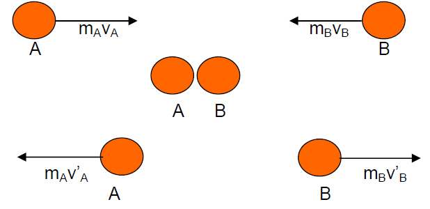
electron A electron B
Momentum space
The linearity of the transducer is an important trait in a transducer. If a transducer is linear, so if the input is doubled, then the output - for example - to be doubled also. This will certainly make it easier to understand and take advantage of the transducer.
Non linearity at least can be divided into two, the non linearity of the known and the unknown. Nonlinearity of the unknown is certainly very difficult, because the connection input - output is unknown. Had this kind of transducer is used as a measuring tool, when input is doubled, then the output to be doubled or tripled, or others, is not known. So for this kind of transducer, separate research needs to be done to get the inputs-output relationship, before use.
As for all non linearity is not known, the transducer that has the character of this kind can still be used to avoid non linearity to her or to do some transformations on the formulas that connect the input to the output. Examples of known non linearity for example: the die area (dead zone), saturation (saturation), logarithmic, quadratic, and so on. The details are as follows:
Die area (dead zone) Transducers
Die area (dead zone) means when it has been granted input, output does not exist. Only after passing a certain threshold value, there is output that is proportional to the input.
Regional Graph Dead (dead zone) Transducers
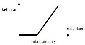 keluaran = output
masukan = input
nilai ambang = threshold value
saturation transducers
Saturation point is, when the input was raised up to a certain value, the output is not growing, but only showed a constant value.
Graph Saturation (saturation) Transducers
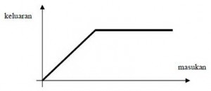 keluaran = output ; masukan = input
 logarithmically transducers
Logarithmically, that is - as the name suggests - when input grows linearly, the output grew logarithmically.
Value kuadratis Transducers
Kuadratis, that is - as the name suggests - when input grows linearly, the output grew by quadratic. In real conditions, the transducer is linear in a broad range very rare. Even a lot of the transducer has a linear nature of which is a combination of several properties are not linear. Therefore, it needs the right tips to take advantage of the phenomenon.
X . I
Terms Sensor and Transducer
Sensor is a device used to detect symptoms or signals originating from a change of energy such as electric energy, physical energy, chemical energy, biological energy, mechanical energy and so on. example; Camera as vision sensors, as sensors hearing ear, the skin as a touch sensor, LDR (light dependent resistance) as a light sensor, and more.
The sensor and transducer is a device or component that has an important role in a system of automatic settings. The accuracy and appropriateness in selecting a sensor will determine the performance of the system settings automatically.General characteristic Sensors and Transducers
In selecting equipment sensors and transducers are appropriate and in accordance with the system to be censored is necessary to note the general requirements of the following sensors:1. Linearity Sensor / Transducer
There are many sensors that generate output signals that vary continuously in response to the continuously changing inputs. For example, a heat sensor can generate a voltage in accordance with the heat felt. In such cases, usually it is known exactly how changes in output compared with the input in the form of a graph. The following figure shows the relationship of two different heat sensors. The straight line in the figure (a). shows a linear response, whereas in figure (b). is a non-linear response.
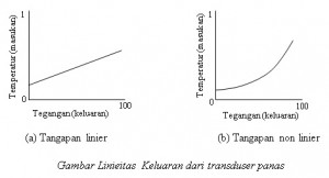
linear response = tanggapan linier
tanggapan non linier = non linier respons
II . Sensitivity Sensor / Transducer
Sensitivity will show how far the sensitivity of the sensor to the measured quantity. Sensitivity is often also expressed with numbers that indicate the "change unit output than input change". and then heat sensor may have a sensitivity that is expressed by "one volt per degree", which means a change of one degree in input will result in a change of one volt outputs. Other heat sensors may have sensitivity "two volts per degree", which means it has sensitivity twice from the first sensor. The linearity of the sensor also affects the sensitivity of the sensor. If the linear response, the sensitivity will be the same for the whole measurement range. image sensor with feedback (b) above will be more sensitive to high temperatures than at low temperatures.3. Response Time Sensor / Transducer
The response time of the sensor shows how fast response to input changes. For example, an instrument with a frequency response that is ugly is a mercury thermometer. The input and the output is the temperature mercury positions. Suppose the temperature changes occur gradually and continuously over time, as shown in figure (a) below.
Frequency is the number of cycles in one second and is given in hertz (Hz). {1 hertz means one cycle per second, 1 kilohertz means 1000 cycles per second]. At low frequencies, which is when the temperature changes slowly, the thermometer will follow the change by "faithful". But when the temperature changes very quickly see figure (b) under then not expected to see a big change in a mercury thermometer, because he is slow and will only show average temperatures.
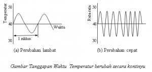
perubahan cepat = rapid change
perubahan lambat = slow changes
There are various ways to express the frequency response of a sensor. For example "one milivolts at 500 hertz". Frequency response can also be expressed as "decibel (db)", which is to compare the output power at a particular frequency with output power at the reference frequency.
X . II
Mathematic linierity
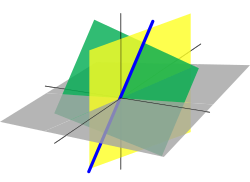
The three-dimensional Euclidean space R3 is a vector space, and lines and planes passing through the origin are vector subspaces in R3.
Linear algebra is the branch of mathematics concerning vector spaces and linear mappings between such spaces. It includes the study of lines, planes, and subspaces, but is also concerned with properties common to all vector spaces.
The set of points with coordinates that satisfy a linear equation forms a hyperplane in an n-dimensional space. The conditions under which a set of n hyperplanes intersect in a single point is an important focus of study in linear algebra. Such an investigation is initially motivated by a system of linear equations containing several unknowns. Such equations are naturally represented using the formalism of matrices and vectors.
Linear algebra is central to both pure and applied mathematics. For instance, abstract algebra arises by relaxing the axioms of a vector space, leading to a number of generalizations. Functional analysis studies the infinite-dimensional version of the theory of vector spaces. Combined with calculus, linear algebra facilitates the solution of linear systems of differential equations.
Techniques from linear algebra are also used in analytic geometry, engineering, physics, natural sciences, computer science, computer animation, advanced facial recognition algorithms and the social sciences (particularly in economics). Because linear algebra is such a well-developed theory, nonlinear mathematical models are sometimes approximated by linear models.
History
The study of linear algebra first emerged from the study of determinants, which were used to solve systems of linear equations. Determinants were used by Leibniz in 1693, and subsequently, Gabriel Cramer devised Cramer's Rule for solving linear systems in 1750. Later, Gauss further developed the theory of solving linear systems by using Gaussian elimination, which was initially listed as an advancement in geodesy.The study of matrix algebra first emerged in England in the mid-1800s. In 1844 Hermann Grassmann published his "Theory of Extension" which included foundational new topics of what is today called linear algebra. In 1848, James Joseph Sylvester introduced the term matrix, which is Latin for "womb". While studying compositions of linear transformations, Arthur Cayley was led to define matrix multiplication and inverses. Crucially, Cayley used a single letter to denote a matrix, thus treating a matrix as an aggregate object. He also realized the connection between matrices and determinants, and wrote "There would be many things to say about this theory of matrices which should, it seems to me, precede the theory of determinants".
In 1882, Hüseyin Tevfik Pasha wrote the book titled "Linear Algebra". The first modern and more precise definition of a vector space was introduced by Peano in 1888; by 1900, a theory of linear transformations of finite-dimensional vector spaces had emerged. Linear algebra took its modern form in the first half of the twentieth century, when many ideas and methods of previous centuries were generalized as abstract algebra. The use of matrices in quantum mechanics, special relativity, and statistics helped spread the subject of linear algebra beyond pure mathematics. The development of computers led to increased research in efficient algorithms for Gaussian elimination and matrix decompositions, and linear algebra became an essential tool for modelling and simulations.
The origin of many of these ideas is discussed in the articles on determinants and Gaussian elimination.
Educational history
Linear algebra first appeared in American graduate textbooks in the 1940s and in undergraduate textbooks in the 1950s. Following work by the School Mathematics Study Group, U.S. high schools asked 12th grade students to do "matrix algebra, formerly reserved for college" in the 1960s. In France during the 1960s, educators attempted to teach linear algebra through affine dimensional vector spaces in the first year of secondary school. This was met with a backlash in the 1980s that removed linear algebra from the curriculum. In 1993, the U.S.-based Linear Algebra Curriculum Study Group recommended that undergraduate linear algebra courses be given an application-based "matrix orientation" as opposed to a theoretical orientation. Reviews of the teaching of linear algebra call for stress on visualization and geometric interpretation of theoretical ideas, and to include the jewel in the crown of linear algebra, the singular value decomposition (SVD), as 'so many other disciplines use it'. To better suit 21st century applications, such as data mining and uncertainty analysis, linear algebra can be based upon the SVD instead of Gaussian Elimination.Scope of study
Vector spaces
The main structures of linear algebra are vector spaces. A vector space over a field F is a set V together with two binary operations. Elements of V are called vectors and elements of F are called scalars. The first operation, vector addition, takes any two vectors v and w and outputs a third vector v + w. The second operation, scalar multiplication, takes any scalar a and any vector v and outputs a new vector av. The operations of addition and multiplication in a vector space must satisfy the following axioms. In the list below, let u, v and w be arbitrary vectors in V, and a and b scalars in F.| Axiom | Signification |
| Associativity of addition | u + (v + w) = (u + v) + w |
| Commutativity of addition | u + v = v + u |
| Identity element of addition | There exists an element 0 ∈ V, called the zero vector, such that v + 0 = v for all v ∈ V. |
| Inverse elements of addition | For every v ∈ V, there exists an element −v ∈ V, called the additive inverse of v, such that v + (−v) = 0 |
| Distributivity of scalar multiplication with respect to vector addition | a(u + v) = au + av |
| Distributivity of scalar multiplication with respect to field addition | (a + b)v = av + bv |
| Compatibility of scalar multiplication with field multiplication | a(bv) = (ab)v [nb 1] |
| Identity element of scalar multiplication | 1v = v, where 1 denotes the multiplicative identity in F. |
Linear transformations
Main article: Linear map
Similarly as in the theory of other algebraic structures, linear
algebra studies mappings between vector spaces that preserve the
vector-space structure. Given two vector spaces V and W over a field F, a linear transformation (also called linear map, linear mapping or linear operator) is a mapAdditionally for any vectors u, v ∈ V and scalars a, b ∈ F:
Linear transformations have geometric significance. For example, 2 × 2 real matrices denote standard planar mappings that preserve the origin.
Subspaces, span, and basis
Again, in analogue with theories of other algebraic objects, linear algebra is interested in subsets of vector spaces that are themselves vector spaces; these subsets are called linear subspaces. For example, both the range and kernel of a linear mapping are subspaces, and are thus often called the range space and the nullspace; these are important examples of subspaces. Another important way of forming a subspace is to take a linear combination of a set of vectors v1, v2, ..., vk:A linear combination of any system of vectors with all zero coefficients is the zero vector of V. If this is the only way to express the zero vector as a linear combination of v1, v2, ..., vk then these vectors are linearly independent. Given a set of vectors that span a space, if any vector w is a linear combination of other vectors (and so the set is not linearly independent), then the span would remain the same if we remove w from the set. Thus, a set of linearly dependent vectors is redundant in the sense that there will be a linearly independent subset which will span the same subspace. Therefore, we are mostly interested in a linearly independent set of vectors that spans a vector space V, which we call a basis of V. Any set of vectors that spans V contains a basis, and any linearly independent set of vectors in V can be extended to a basis. It turns out that if we accept the axiom of choice, every vector space has a basis; nevertheless, this basis may be unnatural, and indeed, may not even be constructible. For instance, there exists a basis for the real numbers, considered as a vector space over the rationals, but no explicit basis has been constructed.
Any two bases of a vector space V have the same cardinality, which is called the dimension of V. The dimension of a vector space is well-defined by the dimension theorem for vector spaces. If a basis of V has finite number of elements, V is called a finite-dimensional vector space. If V is finite-dimensional and U is a subspace of V, then dim U ≤ dim V. If U1 and U2 are subspaces of V, then
.
Matrix theory
Main article: Matrix (mathematics)
A particular basis {v1, v2, ..., vn} of V allows one to construct a coordinate system in V: the vector with coordinates (a1, a2, ..., an) is the linear combinationThere is an important distinction between the coordinate n-space Rn and a general finite-dimensional vector space V. While Rn has a standard basis {e1, e2, ..., en}, a vector space V typically does not come equipped with such a basis and many different bases exist (although they all consist of the same number of elements equal to the dimension of V).
One major application of the matrix theory is calculation of determinants, a central concept in linear algebra. While determinants could be defined in a basis-free manner, they are usually introduced via a specific representation of the mapping; the value of the determinant does not depend on the specific basis. It turns out that a mapping has an inverse if and only if the determinant has an inverse (every non-zero real or complex number has an inverse). If the determinant is zero, then the nullspace is nontrivial. Determinants have other applications, including a systematic way of seeing if a set of vectors is linearly independent (we write the vectors as the columns of a matrix, and if the determinant of that matrix is zero, the vectors are linearly dependent). Determinants could also be used to solve systems of linear equations (see Cramer's rule), but in real applications, Gaussian elimination is a faster method.
Eigenvalues and eigenvectors
Main article: Eigenvalues and eigenvectors
In general, the action of a linear transformation may be quite
complex. Attention to low-dimensional examples gives an indication of
the variety of their types. One strategy for a general n-dimensional
transformation T is to find "characteristic lines" that are invariant sets under T. If v is a non-zero vector such that Tv is a scalar multiple of v, then the line through 0 and v is an invariant set under T and v is called a characteristic vector or eigenvector. The scalar λ such that Tv = λv is called a characteristic value or eigenvalue of T.To find an eigenvector or an eigenvalue, we note that
Inner-product spaces
Main article: Inner product space
Besides these basic concepts, linear algebra also studies vector spaces with additional structure, such as an inner product. The inner product is an example of a bilinear form, and it gives the vector space a geometric structure by allowing for the definition of length and angles. Formally, an inner product is a map- Conjugate symmetry:
- Linearity in the first argument:
-
with equality only for v = 0.
Two vectors are orthogonal if
 .
An orthonormal basis is a basis where all basis vectors have length 1
and are orthogonal to each other. Given any finite-dimensional vector
space, an orthonormal basis could be found by the Gram–Schmidt procedure. Orthonormal bases are particularly nice to deal with, since if v = a1 v1 + ... + an vn, then
  .
.The inner product facilitates the construction of many useful concepts. For instance, given a transform T, we can define its Hermitian conjugate T* as the linear transform satisfying
Some main useful theorems
- A matrix is invertible, or non-singular, if and only if the linear map represented by the matrix is an isomorphism.
- Any vector space over a field F of dimension n is isomorphic to Fn as a vector space over F.
- Corollary: Any two vector spaces over F of the same finite dimension are isomorphic to each other.
- A linear map is an isomorphism if and only if the determinant is nonzero.
Applications
Because of the ubiquity of vector spaces, linear algebra is used in many fields of mathematics, natural sciences, computer science, and social science. Below are just some examples of applications of linear algebra.Solution of linear systems
Main article: System of linear equations
Linear algebra provides the formal setting for the linear combination
of equations used in the Gaussian method. Suppose the goal is to find
and describe the solution(s), if any, of the following system of linear
equations:In the example, x is eliminated from L2 by adding (3/2)L1 to L2. x is then eliminated from L3 by adding L1 to L3. Formally:
The last part, back-substitution, consists of solving for the known in reverse order. It can thus be seen that
We can, in general, write any system of linear equations as a matrix equation:
 .
If the number of variables is equal to the number of equations, then we
can characterize when the system has a unique solution: since N is trivial if and only if det A ≠ 0, the equation has a unique solution if and only if det A ≠ 0.
.
If the number of variables is equal to the number of equations, then we
can characterize when the system has a unique solution: since N is trivial if and only if det A ≠ 0, the equation has a unique solution if and only if det A ≠ 0.Least-squares best fit line
The least squares method is used to determine the best fit line for a set of data. This line will minimize the sum of the squares of the residuals.Fourier series expansion
Fourier series are a representation of a function f: [−π, π] → R as a trigonometric series:The space of all functions that can be represented by a Fourier series form a vector space (technically speaking, we call functions that have the same Fourier series expansion the "same" function, since two different discontinuous functions might have the same Fourier series). Moreover, this space is also an inner product space with the inner product
 ; that is,
Quantum mechanics
Quantum mechanics is highly inspired by notions in linear algebra. In quantum mechanics, the physical state of a particle is represented by a vector, and observables (such as momentum, energy, and angular momentum) are represented by linear operators on the underlying vector space. More concretely, the wave function of a particle describes its physical state and lies in the vector space L2 (the functions φ: R3 → C such that is finite), and it evolves according to the Schrödinger equation. Energy is represented as the operator
  , where V is the potential energy. H is also known as the Hamiltonian operator. The eigenvalues of H
represents the possible energies that can be observed. Given a particle
in some state φ, we can expand φ into a linear combination of
eigenstates of H. The component of H in each eigenstate
determines the probability of measuring the corresponding eigenvalue,
and the measurement forces the particle to assume that eigenstate (wave
function collapse).
, where V is the potential energy. H is also known as the Hamiltonian operator. The eigenvalues of H
represents the possible energies that can be observed. Given a particle
in some state φ, we can expand φ into a linear combination of
eigenstates of H. The component of H in each eigenstate
determines the probability of measuring the corresponding eigenvalue,
and the measurement forces the particle to assume that eigenstate (wave
function collapse).Geometric introduction
Many of the principles and techniques of linear algebra can be seen in the geometry of lines in a real two dimensional plane E. When formulated using vectors and matrices the geometry of points and lines in the plane can be extended to the geometry of points and hyperplanes in high-dimensional spaces.Point coordinates in the plane E are ordered pairs of real numbers, (x,y), and a line is defined as the set of points (x,y) that satisfy the linear equation
Homogeneous coordinates identify the plane E with the z = 1 plane in three dimensional space. The x−y coordinates in E are obtained from homogeneous coordinates y = (y1, y2, y3) by dividing by the third component (if it is nonzero) to obtain y = (y1/y3, y2/y3, 1).
The linear equation, λ, has the important property, that if x1 and x2 are homogeneous coordinates of points on the line, then the point αx1 + βx2 is also on the line, for any real α and β.
Now consider the equations of the two lines λ1 and λ2,
It is interesting to consider the case of three lines, λ1, λ2 and λ3, which yield the matrix equation,
Introduction to linear transformations
Another way to approach linear algebra is to consider linear functions on the two dimensional real plane E=R2. Here R denotes the set of real numbers. Let x=(x, y) be an arbitrary vector in E and consider the linear function λ: E→R, given byConsider the linear functional a little more carefully. Let i=(1,0) and j =(0,1) be the natural basis vectors on E, so that x=xi+yj. It is now possible to see that
This is true for any pair of vectors used to define coordinates in E. Suppose we select a non-orthogonal non-unit vector basis v and w to define coordinates of vectors in E. This means a vector x has coordinates (α,β), such that x=αv+βw. Then, we have the linear functional
Coordinates relative to a basis
This leads to the question of how to determine the coordinates of a vector x relative to a general basis v and w in E. Assume that we know the coordinates of the vectors, x, v and w in the natural basis i=(1,0) and j =(0,1). Our goal is two find the real numbers α, β, so that x=αv+βw, that isInverse image
The set of points in the plane E that map to the same image in R under the linear functional λ define a line in E. This line is the image of the inverse map, λ−1: R→E. This inverse image is the set of the points x=(x, y) that solve the equation,In order to solve the equation, we first recognize that only one of the two unknowns (x,y) can be determined, so we select y to be determined, and rearrange the equation
The vector p defines the intersection of the line with the y-axis, known as the y-intercept. The vector h satisfies the homogeneous equation,
The set of points of a linear functional that map to zero define the kernel of the linear functional. The line can be considered to be the set of points h in the kernel translated by the vector p.
Since linear algebra is a successful theory, its methods have been developed and generalized in other parts of mathematics. In module theory, one replaces the field of scalars by a ring. The concepts of linear independence, span, basis, and dimension (which is called rank in module theory) still make sense. Nevertheless, many theorems from linear algebra become false in module theory. For instance, not all modules have a basis (those that do are called free modules), the rank of a free module is not necessarily unique, not every linearly independent subset of a module can be extended to form a basis, and not every subset of a module that spans the space contains a basis.
In multilinear algebra, one considers multivariable linear transformations, that is, mappings that are linear in each of a number of different variables. This line of inquiry naturally leads to the idea of the dual space, the vector space V∗ consisting of linear maps f: V → F where F is the field of scalars. Multilinear maps T: Vn → F can be described via tensor products of elements of V∗.
If, in addition to vector addition and scalar multiplication, there is a bilinear vector product V × V → V, the vector space is called an algebra; for instance, associative algebras are algebras with an associate vector product (like the algebra of square matrices, or the algebra of polynomials).
Functional analysis mixes the methods of linear algebra with those of mathematical analysis and studies various function spaces, such as Lp spaces.
Representation theory studies the actions of algebraic objects on vector spaces by representing these objects as matrices. It is interested in all the ways that this is possible, and it does so by finding subspaces invariant under all transformations of the algebra. The concept of eigenvalues and eigenvectors is especially important.
Algebraic geometry considers the solutions of systems of polynomial equations.
There are several related topics in the field of Computer Programming that utilizes much of the techniques and theorems Linear Algebra encompasses and refers to.
X . III
Linier equation over a ring
In algebra, linear equations and systems of linear equations over a field are widely studied. "Over a field" means that the coefficients of the equations and the solutions that one is looking for belong to a given field, commonly the real or the complex numbers. This article is devoted to the same problems where "field" is replaced by "commutative ring", or, typically "Noetherian integral domain".
In the case of a single equation, the problem splits in two parts. First, the ideal membership problem, which consists, given a non homogeneous equation
 and b in a given ring R, to decide if it has a solution with
  in R, and, if any, to provide one. This amounts to decide if b belongs to the ideal generated by the ai. The simplest instance of this problem is, for k = 1 and b = 1, to decide if a is a unit in R.
The syzygy problem consists, given k elements
 in R, to provide a system of generators of the module of the syzygies of
  that is a system of generators of the submodule of those elements
  in Rk that are solution of the homogeneous equation
Given a solution of the ideal membership problem, one obtains all the solutions by adding to it the elements of the module of syzygies. In other words, all the solutions are provided by the solution of these two partial problems.
In the case of several equations, the same decomposition into subproblems occurs. The first problem becomes the submodule membership problem. The second one is also called the syzygy problem.
A ring such that there are algorithms for the arithmetic operations (addition, subtraction, multiplication) and for the above problems may be called a computable ring, or effective ring. One may also say that linear algebra on the ring is effective.
The article considers the main rings for which linear algebra is effective.
Generalities
To be able of solving the syzygy problem, it is necessary that the module of syzygies is finitely generated, because it is impossible to output an infinite list. Therefore the problems considered here make sense only for Noetherian rings, or at least a coherent ring. In fact, this article is restricted to Noetherian integral domains because of the following result.Given a Noetherian integral domain, if there are algorithms to solve the ideal membership problem and the syzygies problem for a single equation, then one may deduce from them algorithms for the similar problems concerning systems of equations.
This theorem is useful to prove the existence of algorithms. However, in practice, the algorithms for the systems are designed directly, as it is done for the systems of linear equations over a field.
Properties of effective rings
Let R be an effective commutative ring.- There is an algorithm for testing if an element a is a zero divisor: this amounts to solve the linear equation ax = 0.
- There is an algorithm for testing if an element a is a unit, and if it is, computing its inverse: this amounts to solve the linear equation ax = 1.
- Given an ideal I generated by a1, ..., ak, there is an algorithm for testing if two elements of R have the same image in R/I, and linear algebra is effective over R/I: testing the equality of the images of a and b amounts to solve the equation a = b + a1z1 + ⋅⋅⋅ + akzk; for solving a linear system over R/I, it suffices to write it over R and to add to one side of the ith equation a1zi,1 + ⋅⋅⋅ + akzi,k (for i = 1, ...), where the zi,j are new unknowns.
Linear equations over the integers or a principal ideal domain
There are algorithms to solve all the problems addressed in this article over the integers. In other words, linear algebra is effective over the integers. See Linear Diophantine system for details.The same solution applies to the same problems over a principal ideal domain, with the following modifications.
The notion of unimodular matrix of integers must be extended by calling unimodular a matrix over a integral domain whose determinant is a unit. This means that the determinant is invertible and implies that unimodular matrices are the invertible matrices such all entries of the inverse matrix belong to the domain.
To have an algorithmic solution of linear systems, a solution for a single linear equation in two unknowns is clearly required. In the case of the integers, such a solution is provided by extended Euclidean algorithm. Thus one needs that, for the considered principal ideal domain, there is an algorithm with a similar specification as the extended Euclidean algorithm. That is, given a and b in the principal ideal domain, there is an algorithm computing a unimodular matrix
The main case where this is commonly used is the case of linear systems over the ring of univariate polynomials over a field. In this case, the extended Euclidean algorithm may be used. See polynomial greatest common divisor#Bézout's identity and extended GCD algorithm for details.


![f(x)={\frac {a_{0}}{2}}+\sum _{n=1}^{\infty }\,[a_{n}\cos(nx)+b_{n}\sin(nx)].](https://wikimedia.org/api/rest_v1/media/math/render/svg/7bfd233836a00d8972d09c8ed15fd5f147e0cb64)

![\langle f,h_{k}\rangle ={\frac {a_{0}}{2}}\langle h_{0},h_{k}\rangle +\sum _{n=1}^{\infty }\,[a_{n}\langle h_{n},h_{k}\rangle +b_{n}\langle \ g_{n},h_{k}\rangle ],](https://wikimedia.org/api/rest_v1/media/math/render/svg/5d92a3ed77d3938b339f063f9ff10dc4d7ac860e)


Tidak ada komentar:
Posting Komentar