Transistors in pure electronics engineering are informed in various forms as electronic relays, as drivers, as sinus amplifiers, as electronic mechanical functions, as electronic jumper, as a tool of electronic mathematical functions in operational amplifiers, and as electronics transformers thus the electronics busbar function .

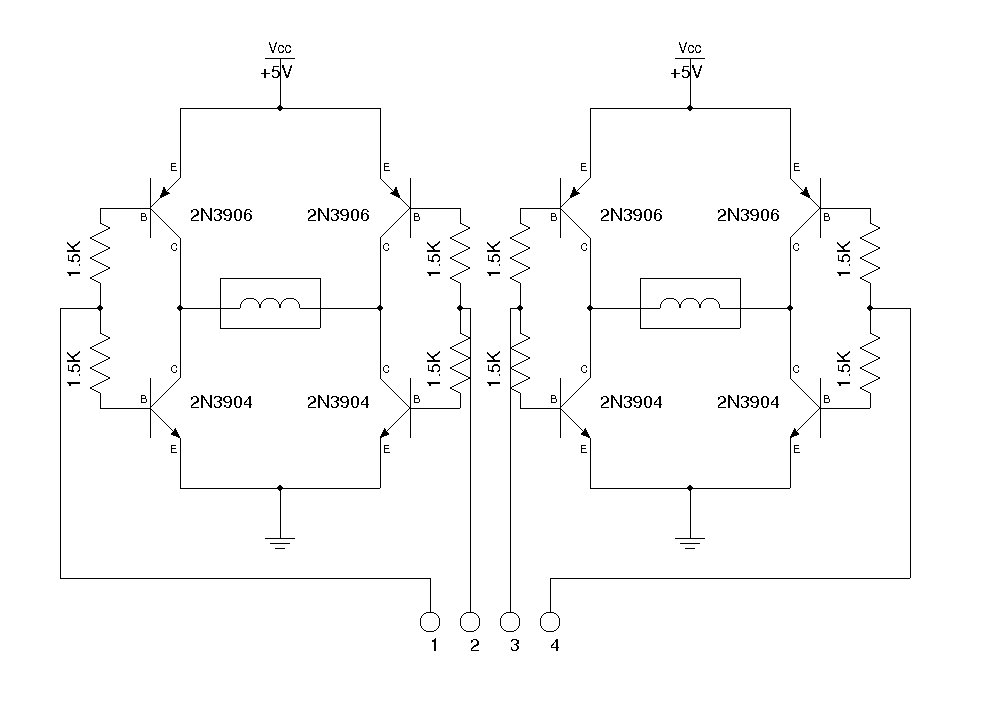
H-BRIDGE These circuits reverse a motor via two input lines. Both inputs must not be LOW with the first H-bridge circuit. If both inputs go LOW at the same time, the transistors will "short-out" the supply. This means you need to control the timing of the inputs. In addition, the current capability of some H-bridges is limited by the transistor types.

The driver transistors are in "emitter follower" mode in this circuit.

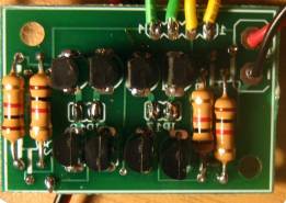
Two H-Bridges on a PC board

H-Bridge using Darlington transistors

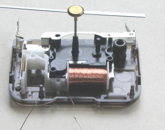
HEX BUG
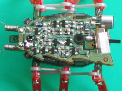
This is the circuit from a HEX BUG. It is a surface-mount bug with 6 legs. The pager motor is driven by an H-Bridge and "walks" to a wall where a feeler (consisting of a spring with a stiff wire down the middle) causes the motor to reverse.
In the forward direction, both sets of legs are driven by the compound gearbox but when the motor is reversed, the left legs do not operate as they are connected by a clutch consisting of a spring-loaded inclined plane that does not operate in reverse.
This causes the bug to turn around slightly.
The circuit also responds to a loud clap. The photo shows the 9 transistors and accompanying components:

HEX BUG CIRCUIT

Inclined Dog Clutch

HEX BUG GEARBOX

Hex Bug gearbox consists of a compound gearbox with output "K" (eccentric pin) driving the legs. You will need to see the project to understand how the legs operate.
When the motor is reversed, the clutch "F" is a housing that is spring-loaded to "H" and drives "H via a square shaft "G". Gearwheel "C" is an idler and the centre of "F" is connected to "E" via the shaft. When "E" reverses, the centre of "F" consists of a driving inclined plane and pushes "F" towards "H" in a clicking motion. Thus only the right legs reverse and the bug makes a turn. When "E" is driven in the normal direction, the centre of "F" drives the outer casing "F" via an action called an "Inclined Dog Clutch" and "F" drives "G" via a square shaft and "G" drives "H" and "J" is an eccentric pin to drive the legs.
The drawing of an Inclined Dog Clutch shows how the clutch drives in only one direction. In the reverse direction it rides up on the ramp and "clicks" once per revolution. The spring "G" in the photo keeps the two halves together.

MODEL RAILWAY TIME Here is a simpler circuit than MAKE TIME FLY from our first book of 100 transistor circuits.
For those who enjoy model railways, the ultimate is to have a fast clock to match the scale of the layout. This circuit will appear to "make time fly" by revolving the seconds hand once every 6 seconds. The timing can be adjusted by the electrolytics in the circuit. The electronics in the clock is disconnected from the coil and the circuit drives the coil directly. The circuit takes a lot more current than the original clock (1,000 times more) but this is the only way to do the job without a sophisticated chip.

Model Railway Time Circuit Connecting the circuit to the clock coil

For those who want the circuit to take less current, here is a version using a Hex Schmitt Trigger chip:

Model Railway Time Circuit using a 74c14 Hex Schmitt Chip

SLOW START-STOP To make a motor start slowly and slow down slowly, this circuit can be used. The slide switch controls the action. The Darlington transistor will need a heatsink if the motor is loaded.

Slow Start-Stop Circuit

THE DARLINGTON TRANSISTOR Normally a single transistor-stage produces a gain of about 100.
If you require a very high gain, two stages can be used. Two transistors can be connected connected in many ways and the simplest is DIRECT COUPLING. This is shown in the circuit below. An even simpler method is to combine two transistors in one package to form a single transistor with very high gain, called DARLINGTON TRANSISTOR.
These are available as:
BD679 NPN-Darlington
2N6284 NPN-Darlington
BC879 NPN-Darlington
BC880 PNP-Darlington TIP122 NPN-Darlington
TIP127 PNP-Darlington
These devices consist of two NPN or PNP transistors but the same result can be obtained by using a PNP/NPN pair. This is called a Sziklai pair. This arrangement will have to be created with two separate transistors.
The Darlington transistor can also be referred to as:
"Super Transistor, Super Alpha Pair, Sziklai pair, Complementary Pair,
Darlington transistors have a gain of 1,000 to 30,000. When the gain is 1,000:1 an input of 1mA will produce a current of 1 amp in the collector-emitter circuit.
The only disadvantage of a Darlington Transistor is the minimum voltage between collector-emitter when fully saturated. It is 0.6v to 1.5v depending on the current through the transistor.
A normal transistor has a collector-emitter voltage (when saturated) of 0.2v to 0.5v. The higher voltage means the transistor will heat up more and requires good heatsinking. In addition, a Darlington transistor needs 1.2v between base and emitter before it will turn on. A Sziklai pair only requires 0.6v for it to turn on.

This circuit detects movement and operates a relay. The PIR module has "Sensitivity" and "Time Delay" pots. They can be purchased on eBay for $2.71 including postage!

H-Bridges: Theory and Practice

Introduction

A number of web sites talk about H-bridges, they are a topic of great discussion in robotics clubs and they are the bane of many robotics hobbyists. I periodically chime in on discussions about them, and while not an expert by a long shot I've built a few over the years. Further, they were one of my personal stumbling blocks when I was first getting into robotics. This attention of the notebook is devoted to the theory and practice of building H-bridges for controlling brushed DC motors (the most common kind you will find in hobby robotics ...) I've got an image of one below with both as a unit and "expanded" in an exploded view.

Basic Theory

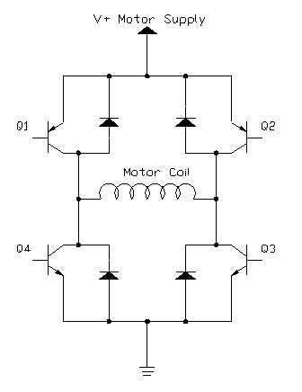
Let's start with the name, H-bridge. Sometimes called a "full bridge" the H-bridge is so named because it has four switching elements at the "corners" of the H and the motor forms the cross bar. The basic bridge is shown in the figure to the right.

Of course the letter H doesn't have the top and bottom joined together, but hopefully the picture is clear. This is also something of a theme of this tutorial where I will state something, and then tell you it isn't really true :-).

The key fact to note is that there are, in theory, four switching elements within the bridge. These four elements are often called, high side left, high side right, low side right, and low side left (when traversing in clockwise order).

The switches are turned on in pairs, either high left and lower right, or lower left and high right, but never both switches on the same "side" of the bridge. If both switches on one side of a bridge are turned on it creates a short circuit between the battery plus and battery minus terminals. This phenomena is called shoot through in the Switch-Mode Power Supply (SMPS) literature. If the bridge is sufficiently powerful it will absorb that load and your batteries will simply drain quickly. Usually however the switches in question melt.

To power the motor, you turn on two switches that are diagonally opposed. In the picture to the right, imagine that the high side left and low side right switches are turned on. The current flow is shown in green.

The current flows and the motor begins to turn in a "positive" direction. What happens if you turn on the high side right and low side left switches? You guessed it, current flows the other direction through the motor and the motor turns in the opposite direction.

Pretty simple stuff right? Actually it is just that simple, the tricky part comes in when you decide what to use for switches. Anything that can carry a current will work, from four SPST switches, one DPDT switch, relays, transistors, to enhancement mode power MOSFETs.

One more topic in the basic theory section, quadrants. If each switch can be controlled independently then you can do some interesting things with the bridge, some folks call such a bridge a "four quadrant device" (4QD get it?). If you built it out of a single DPDT relay, you can really only control forward or reverse. You can build a small truth table that tells you for each of the switch's states, what the bridge will do. As each switch has one of two states, and there are four switches, there are 16 possible states. However, since any state that turns both switches on one side on is "bad" (smoke issues forth), there are in fact only four useful states (the four quadrants) where the transistors are turned on.

High Side Left	High Side Right	Lower Left	Lower Right	Quadrant Description

On	Off	Off	On	Motor goes Clockwise
Off	On	On	Off	Motor goes Counter-clockwise
On	On	Off	Off	Motor "brakes" and decelerates
Off	Off	On	On	Motor "brakes" and decelerates

The last two rows describe a maneuver where you "short circuit" the motor which causes the motors generator effect to work against itself. The turning motor generates a voltage which tries to force the motor to turn the opposite direction. This causes the motor to rapidly stop spinning and is called "braking" on a lot of H-bridge designs.

Of course there is also the state where all the transistors are turned off. In this case the motor coasts if it was spinning and does nothing if it was doing nothing.

Using the H-Bridge

Layout Considerations

Generally this circuit is fairly free of layout restrictions, however there are some things that you can do to make your life easier. A sample layout is shown below.

One of the things to note is that the transistors are arranged "back to back" with their tabs facing each other. In my layout I have spaced them 3/8" apart which allows me to put a piece of 1" x 3/8" x copper bar stock down the middle and with #4-40 machine bolts to secure it. A 1 - 1/2" piece of this stock weighs about 3 oz. This basically doubles to current capacity of the bridge, and if you then bolt the copper bar to a metal enclosure you can triple the capacity to a full 6 amps continuous duty. Further, the two left transistors are the "upper" source transistors and the two right transistors are the lower "sink" transistors. That means that any thermal solution will have heat being injected from diagonal corners which further maximizes the benefit by spreading out the heat injection. The point here is to think about whether or not you are going to put heat sinks on the transistors and lay them out accordingly.

Alternatively you can build this bridge on a piece of perfboard and just solder it together. Be sure and use at least 18 ga wire on the legs of the transistors.

Microprocessor Control

To use this h-bridge with a microprocessor, you must connect the three control lines to output pins on the microprocessor. Using the BasicStamp II as an example, consider the following hookup diagram.

As you can see three pins from the Basic Stamp are connected to each H-bridge board. In this example they are P0, P1, and P2 to the board controlling the left motor and P4, P5, and P6 to the board controlling the right motor. One of the advantages of using three pins that are both right next to each other, and in the same group of four bits (called nybbles) is that you can use a single variable (one of OUTA, OUTB, OUTC, or OUTD) to write to four pins at once.

This is really only important on chips like the BASIC Stamp where their can be a millisecond or more between the execution of one instruction and the next. By connecting them this way you can cause both motors to start turning with a single instruction such as this assignment:

OUTL = $33

Whereas if you did two instructions :

OUTA = $03

OUTB = $03

You would find that the left motor started turning first, then the right motor. So on a robot that steered with two motors the motor would make a slight turn to the right, then go straight. If you turned them off in the same sequence you would find that the robot corrected its heading back to the original heading but would not have traveled "straight" ahead. For systems that use gear motors such as the 12V Brevel motors or the Globe motors, this won't be a noticeable problem, but higher performance motors will definitely suffer.

The easiest way to use PWM on the motor is to start with the direction and enable bits "high" or at a logic 1 value. This turns on the high side (source) transistor and leaves the sink side transistor off. You can then send "low" pulses out the ENA* line to turn the motor on and off. This would allow you to use a single 'PWM' output, such as the one that is available on the PIC16F628, to control the PWM duty cycle in hardware while the PIC managed other aspects of controlling the motor. The most common use would be to provide encoder feedback into the PIC that would allow a simple PID algorithm to be implemented. With two bits of encoder input, three bits of motor control, and two bits for serial I/O the 16F628 would be well engaged.

Transistor Stepper Motor Driver

Driving Bipolar Stepper Motors

THE
H-BRIDGE

The H-Bridge is designed to drive a motor clockwise and anticlockwise.
To reverse a motor, the supply must be reversed and this is what the H-Bridge does.
An H-Bridge can be made with SWITCHES, RELAYS, TRANSISTORS or MOSFETS.
Some circuits are just demonstration circuits and need "damper diodes" (protection diodes) to reduce spikes. H-Bridge with switches:

Do not make circuit "A." It can easily create a SHORT-CIRCUIT. It is only a demonstration circuit.

Switch A and D will make the motor rotate clockwise.
Switch B and C will make the motor rotate anti-clockwise.
Switch A and B will create a BRAKE.
Do not close switch A and C at the same time.
Do not close switch B and D at the same time.

An improved design is shown in Circuit C. It does not create any short-circuit:

H-Bridge with a relay:

The top diagram shows the underside
of a double-pole double-throw relay

The motor is active at all times. Push the button to reverse the direction of rotation. H-Bridge with 2 relays:This circuit has an advantage. It has FORWARD, OFF, REVERSE and BRAKE (off is BRAKE). The relays are single-pole change-over.

The first two circuits above are manual.
For a project such as a robot or car, we need an ELECTRONIC circuit - one that is controlled by a "CONTROL CIRCUIT". The Control Circuit outputs a signal (or a number of signals) to control an H-Bridge.
Here is a circuit of a Hex Bug. The Control Circuit consists of the first 3 transistors. These amplify the signal from the electret microphone and produce a signal that is able to charge a 47u electrolytic. The next two transistors provide inverted signals to the H-Bridge and are part of the Control Circuit. The H-Bridge consists of the last 4 transistors.

THE MOTOR
The type of motor we will be powering is a 3-pole (or 5-pole) with two brushes, similar to the following images:

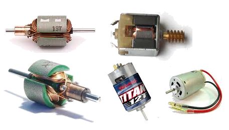
These motors come in different shapes and sizes and have an output from 2,000RPM to more than 16,000RPM.
They operate on less than 1v to more than 24v and the current they require can be less than 100mA to more than 5 amps.
They all have some things in common:
1. They all have a permanent magnet called the FIELD MAGNET.
2. They all rotate in the opposite direction when the supply is reversed.
3. They all take a high current when starting and a lower current when rotating (spinning) at maximum RPM (Revolutions Per Second).
4. They all take a higher current when loaded - (the motor is driving a load). A load may be placing your fingers on the output shaft or driving through a gearbox and lifting a load or driving wheels via a gearbox.
The torque (twisting ability of the output shaft) depends on the voltage and current as well as the strength of the field magnet and the quality of construction (the closeness of the field magnet to the armature).

THREE THINGS
To drive a motor forward and reverse, the circuit must deliver a voltage in one direction, then in the opposite direction.
It must also be able to deliver a "running current" (operating current) (say up to 1 amp) and a "starting current" (up to 5 amps), and a "loaded current" (up to 5 amps). The transistors must be capable of passing a "stalled current" without being destroyed.
The power supply must be capable of delivering a high current so the motor will START-UP under load. THE H-BRIDGE
The circuits we will discuss are called a transistor H-BRIDGE. The active sections of the circuit create the letter "H" to produce the term "H-Bridge."
There are a number of different H-Bridge designs and the actual circuit will depend on the number of transistors, the type of layout, the number of control lines, the voltage of the bridge, and a number of other factors.
That's why we have a number of different designs to cover these variations.DESIGN 1
This design uses 4 transistors. Both inputs must NEVER be HIGH (this will create a short-circuit and damage the transistors). However this circuit is a good design. The voltage on the H-Bridge can be any voltage and the control voltage just needs to be higher than 1v. The circuit provides OFF feature when both inputs are LOW but does not provide BRAKE feature.

DESIGN 2This design uses 6 transistors to do the same job as the circuit above. It does not have any advantages over the circuit above and simply uses extra components. The input voltage must be more than 1.5v for A and B must be higher than 4v to turn off line B. When line B is less than 3.5v, it activates the circuit. The timing of the inputs will prevent any "shoot through" current.

DESIGN 3This design requires the supply voltage to the 74C14 to be the same as the voltage on the H-Bridge (5v to 18v). The circuit provides BRAKE feature when the output of both gates are the same (either HIGH or LOW). There is a "shoot through" current during the time when the inverters change state and this occurs as follows:
When the output of the gate is low, the bottom transistor is not turned on but the top transistor is fully turned ON. When the output of the inverter rises, the top transistor is ON and the lower transistor is also turned on. When the inverter is HIGH, the top transistor is turned OFF. During the time when the inverter is changing from LOW to HIGH, both transistors are turned ON.
The HIGH on the motor will be rail voltage minus the collector-emitter voltage (about 0.3v). The total voltage-drop to the motor will be about 0.6v.

DESIGN 4This circuit does not have the "shoot through" current during the time when the inverters change state but it does not have the same performance as the circuit above. The voltage on the IC and H-Bridge must be the same. The transistors are EMITTER FOLLOWERS and the voltage on the motor will be less than the voltages on the circuit above because the HIGH on the motor will be determined by the output voltage of the IC, minus the slight drop across the 1k and the voltage drop across the base-emitter junction of the transistor (a total of about 1v). The total voltage drop to the motor (due to both sides of the bridge) will be about 2v.
The circuit is only suitable for a low-current motor as the 74C14 can only supply 10mA and the 1k base resistors will limit the current available through the transistors. The resistors can be reduced to 470R.

DESIGN 5This circuit requires 4 inputs and the HIGH inputs must be about 12v. The LOW inputs need to be as close to 0v as possible. With correct timing of the inputs, no "shoot-through" current will be produced.

DESIGN 6This circuit uses a combination of MOSFETs and transistors:
Input A HIGH, Input D HIGH - forward rotation
Input B HIGH, Input C HIGH - reverse rotation
Input A HIGH, Input B HIGH - not allowed
Input C HIGH, Input D HIGH - not allowed

DESIGN 7This circuit controls the speed of a 12v drill and drives a MOSFET. The H-Bridge is a reversing switch (double-pole double-throw). The MOSFET will deliver up to 30Amps. The frequency of the oscillator is in the range 550Hz to about 6.5kHz, with an off period of about 2.6us.

PWM 12v CORDLESS DRILL MOTOR CONTROLLER

DESIGN 8This circuit uses 2 555 IC's to provide forward and reverse motor-control. It does not have an "OFF" position. When pins 2&6 are tied together, the 555 becomes a Schmitt Trigger, detecting when the input is above 2/3 of rail voltage and below 1/3 rail voltage.
The only problem with a 555 is the output voltage on pin 3. It does not rise to rail voltage and does not fall to 0v. The HIGH can be about 1.5v less than rail voltage and the LOW can be 0.7v above the 0v rail. The actual HIGH and LOW from the chip will depend on the supply voltage and the current taken by the load.

DESIGN 9This circuit produces speed control in forward and reverse direction. It does not have an "OFF" position.

DESIGN 10This circuit uses buffer transistors on the output to deliver up to 4 amps to the motor. It does not have an "OFF" position. As mentioned above, the output from a 555 (pin 3) is less than rail voltage and since the BD679 transistors are "emitter followers" they will have at least 2v5 drop across the collector-emitter terminals and thus need heatsinking. The motor will not see more than 8v5. [This is not a very efficient H-Bridge.] The most efficient H-Bridge use transistors in an arrangement shown in Design 1-6 and 15. These arrangements have the lowest voltage-drop across each of the transistors. This means the maximum voltage will be delivered to the motor and thus the motor will produce the maximum torque (power) and will take the maximum current when fully loaded. Even a slight voltage drop to a motor will be noticeable when the motor is under load, so it is important to have a power supply that is capable of delivering a high current and a 'low-loss" H-Bridge.

DESIGN 11This is a half-bridge circuit. It is low-cost and effective. It requires a "split-supply." This is a 6v battery tapped at 3v or two 3v batteries. The input voltage needs to be about 1v. Both inputs must NOT be HIGH at the same time. The circuit has: Forward, OFF, Reverse.

DESIGN 12This circuit uses a half-bridge to dive a motor in the forward/reverse direction. It does not have an "OFF" position.

DESIGN 13This circuit needs just one input-line from a microcontroller to produce forward/reverse. It does not have "OFF" position. The input must be 0v for forward and 5v for reverse.
When we say 0v on "A" we do not mean simply removing the 5v but taking "A" directly to the 0v rail - in other words, "shorting A to 0v." This is done via an output from a previous stage called a DIGITAL STAGE that produces 5v when HIGH and 0v when LOW.

DESIGN 14This circuit uses 4 x BD679 Darlington transistors to drive a motor: Forward - Off - Reverse. Two inputs are needed and both must NOT be HIGH at the same time. It does not have a BRAKE function.

DESIGN 15This circuit is a SOLAR TRACKER. It uses green LEDs to detect the sun and an H-Bridge to drive the motor. A green LED produces nearly 1v but only a fraction of a milliamp when sunlight is detected by the crystal inside the LED and this creates an imbalance in the circuit to drive the motor either clockwise or anticlockwise. The circuit will deliver about 300mA to the motor.
The circuit was designed by RedRok and kits for the Solar Tracker are available from: This design is called: LED5S5V Simplified LED low power tracker.

To select the type of H-Bridge for your particular application, you need to match the H-Bridge inputs with the outputs from your circuit. Some H-Bridges need 1v to activate each leg of the bridge and others need slightly less than rail voltage to activate. In other words, they are active-LOW, but the voltage will need to rise to say 12v to turn the line off.
Some of these requirements are very difficult to achieve, so you should pick a simple design. Some H-Bridge circuits are over-designed - such as using an LM311 comparator to drive each side of the bridge. This can be replaced with a BC547 transistor on each side of the bridge.
In addition, some bridges drop (lose) 1v or more on each leg and this will reduce the power of the motor considerably. The answer is to supply the bridge with a higher voltage. You can supply a motor with a slightly higher voltage and get the maximum performance from the motor. The motor will run much faster on no-load, but you will get the power you need when it is loaded. DESIGN 16
Bidirectional Analog Solar Tracker or Sensor

The circuit uses N channel IRF3708 MOSFETS in the low side and P channel SPP18P06P in the high side.
The pair of BLUE LEDs generate a differential voltage applied to the gates. The diodes cause these voltages to always be above ground. If one side is higher than the other, one IRF3708 MOSFET turns on harder and and enables the SPP18P06P MOSFET on the opposite corner to also turn on causing the motor to turn. If the differential voltage is the other way the motor reverses.

This circuit requires a small bias current be pulled out of the MOSFET gates to compensate for the leakage currents going into the gate from the positive supply which would could cause both MOSFETs to turn on; a bad thing. A pair of resistors could be connect from the gates to the emitters to absorb the approximately 20nA of leakage current. Or you can use diodes that have more leakage current than the MOSFET gates.

The 1N4148 universal high speed switching diode has about 20nA of leakage current; more as the temperature goes up. The reason normal 10MΩ resistors don't work is they consume more current than can be supplied by the BLUE LEDs. Low leakage diodes such as the BAS416 don't work in this circuit is because their leakage current is too low.

DESIGN 17Change-over every 30 seconds
The following circuit pulses a latching relay every 30 seconds. The circuit only consumes current during the 50mS latching period.
The values for the timing components have not been provided. These can be worked out by experimentation.

DESIGN 18High Current H-Bridge-1This circuit will deliver 3 amps to a 12v motor:

DESIGN 19High Current H-Bridge-2 This circuit will deliver up to 3 amps to a 6v motor. Use TIP100 (NPN) and TIP105 (PNP) for 8 amp
H-Bridge. Forward and reverse signals must not be applied at the same time as this will create a SHORT-CIRCUIT. 1N4148 diodes will not be suitable. Use 1N4004 diodes.

DESIGN 20This circuit will operate from a 5v microcontroller and provide forward/reverse/brake. Use TIP31/32 and BC547 transistors. The input transistors work in an unusual way. They are emitter-followers but they have the load in both the collector and emitter circuits.

DESIGN 21

DESIGN 22

This circuit does work however the transistors in the bridge will not provide a high current.
The current-capability of the bridge comes from the ability of the transistor to amplify the current entering their base. Let us consider Q3.
The current entering the base of Q3 via the 1k resistor will only the about 1mA and this means the collector-emitter current will be a maximum of 300mA.
The current-capability of Q6 will be higher.
When Q2 is turned on via the 10k on the base, we will assume the control voltage is 5v and 0.5mA will enter the base of Q2. This will allow 100mA to flow through the collector-emitter terminals of Q2 and this will be adequate to completely turn ON Q6.
The current capability of Q6 is 500mA.
You can see the limitation of the circuit is Q3 and a motor will draw 300mA or more when under load.
To make the circuit more reliable, POWER TRANSISTORS are needed in the bridge. DESIGN 24

This circuit looks very good until you realise the transistors are DARLINGTON and they produce about 2v to 2.5v across the collector-emitter terminals. This means you can lose up to 5v for a 12v supply and the motor will have almost no strength.
In fact the supply can be 1v higher than the motor-voltage to allow for the losses in the bridge and this will give the motor full strength. You can even increase the supply by up to 3v to 5v to produce enormous torque when needed and use PWM to control the speed of the motor (RPM - and thus torque) for all other situations.
For this circuit you can increase the supply by 5v and then add another 3v to 5v to achieve the maximum from the motor.
The use of four optocouplers allows a microcontroller to control the bridge as all the control lines are completely isolated from the bridge.

DESIGNING AN H-BRIDGE To get a motor to start under load requires at least three times the running current. In addition, a motor take 3 times the running current when it is loaded.
That's why an H-Bridge must be able to deliver a HIGH CURRENT.
To deliver a high current, the transistors must be fully SWITCHED ON. In other words they must be fully SATURATED.
To fully saturate a transistor, the base current must be about 1/10 the collector-emitter current.
Most transistors have a gain of about 100 but this only applies when the transistor is passing about 10mA. To get a transistor to pass a high current, the base current must be increased to about 10mA for every 100mA collector-emitter current.
Transistors are not linear devices and that's why this requirement is rarely mentioned.
Most specification-sheets highlight the qualities of a transistor and fail to mention the problems you will encounter.
That's why you have to drive the output transistors in an H-bridge via a DRIVER TRANSISTOR.
The driver transistor will have a gain of about 50 so the input current to the bridge will only be a few milliamps.
The other factor you have to take into consideration is the VOLTAGE-DROPS across each leg of the bridge.
A saturated transistor will drop about 0.3v whereas a Darlington transistor will drop about 1v and a MOSFET will drop only about 0.05v. An emitter-follower will drop about 0.7v
You need to build a test-circuit and measure the voltage drops on each leg before committing to a particular design. The performance of a motor will fall considerably if it does not see full rated voltage.
You can increase the supply voltage to a bridge to account for the voltage-drop across each leg. This will increase the no-load RPM but allow the motor to produce maximum torque.

If you are using MOSFETs, the gate must be at least 0.6v higher than the Source. This is the case with an IRF3708 as it has a very low turn-on for the gate. However many MOSFETS need about 3v before they will start to turn on.
Here is an example of what we mean. The maximum voltage seen by the motor is 9v due to the fact that the top MOSFET needs 3v between the gate and Source, for it to turn on. The Source will be 3v lower than the gate:

CAUTION There are many H-Bridge circuits on the web that do not work, so you have to be careful.

PWM A PWM B T1N4004 1N4004 NPN IRFZ40 NPN IRFZ4o channel 22k ON B ON A BC547 BC547

Build an op amp with three discrete transistors

We can use three discrete transistors to build an operational amplifier with an open-loop gain greater than 1 million (Figure 1). We bias the output at approximately one-half the supply voltage using the combined voltage drops across zener diode D₁, the emitter-base voltage of input transistor Q₁, and the 1V drop across 1-MΩ feedback resistor R₂.

Resistor R₃ and capacitor C₁ form a compensation network that prevents the circuit from oscillating. The values in the figure still provide a good square-wave response. The ratio of R₂ to R₁ determines the inverting gain, which is −10 in this example.

We can configure this op amp as an active filter or as an oscillator. It drives a load of 1 kΩ. The square-wave response is good at 10 kHz, and the output reduces by 3 dB at 50 kHz. Set the 50-Hz low-frequency response with the values of the input and the output capacitors. We can raise the high-frequency response by using faster transistors and doing careful layout.

GOOD JOB GOOD RE ACT ... Developing a flying car

Having been an automotive engineer in flown and driven his prototype "GyroDrive" (Figure 1). watch him fly and drive the car:

Figure 1 The Gyrodrive combines a gasoline-powered gyrocopter with an electric-powered three-wheel motorcycle

Březina must be onto something, since there is another group designing a road-able gyrocopter, the PAL-V Liberty. They have been working on this since 2001, and it shows. The promo video (see below) shows the kind of CAD design and real-world testing any automotive product requires.

The thing is, this is another product that is supposed to go on sale in 2018. They have had a working prototype since 2012. Since it is a 3-wheeled vehicle, it only has to pass motorcycle safety and pollution regulations. There is no crash-testing, which would require a structure with much more weight along with air bags and other design hurdles.

Like a lot of great engineers, they may be reaching for a bridge too far. It’s not only a trike, but a tilting trike. Rather than just lash the rotors like Březina does, it electrically lowers the whole tower and then the rotors can fold back in a method they do not disclose. My dad used to say, “Starts out like a castle, ends up like an outhouse.” I hope PAL-V engineers take out the gee-whiz features and just make a simple basic design that they might be able to sell in 2018. Time will tell.

(Figure 2). Like many impractical projects, there was always another key thing needed. After a while, he said he needed to develop a new rotary engine to get the specific power needed for the car. Then it was computer control to keep the thing stable. Moller has never made a vehicle that flew in untethered flight. Eventually he announced a new design, the M200G Volantor (Figure 3). The TV show Mythbusters estimated that Moller has spent about $200 million on the Skycar.

Figure 2 The Moller M200 (l) and M400 (r) have never flown untethered much less gotten FCC certification, despite 50 years of development

Figure 3 Despite the failure of the Moller Skycar, the company now wants to introduce the M200X Volantor. This is a 5-inch wooden model for sale on eBay

With the advent of electric drones, many people are trying to scale them up for human transport. Amongst these is Google co-founder Larry Page. He has spent 100 million dollars, but at least his flying car (Figure 4) is supposed to come out in 2017. The New York Times said it “... looked like something Luke Skywalker would have built out of spare parts.”

Figure 4 The Kitty Hawk Flyer is supposed to go on sale in 2017 (courtesy Kitty Hawk).

Perhaps more appealing to the Eloi at the Times is the Aeromobil flying car (Figure 5). It’s another complex product with an introduction “just around the corner.” It’s pretty and swoopy, and they claim to be legal in most countries. As a four-wheeled vehicle, it has to pass crash tests, safety tests, and roll-over tests. That is a monumental task just for the bureaucratic nightmare you have to navigate. The real killer is all the weight you have to add. That weight makes everything larger. A pound of payload adds 5 pounds total, even if that payload is airbags or crush structures. Like so many of these schemes, you can pre-order it in 2017.

Figure 5 The AeroMobil s.r.o. is beautiful, but exceedingly complex (courtesy AeroMobil).

At least the folks at Jetpack Aviation have brought a jet-pack product to market. Now they want to hang six electric motors on top of a helicopter cabin and fly through the air (Figure 6). The problem is that it’s not a flying car, it’s a VTOL (vertical take-off and landing) aircraft. It is also a rotorcraft, like any other helicopter. As Bob Dible my RC (radio control) buddy taught me with the Skycar, to actually hover a heavy vehicle like this means noise over 120dB, and very poor specific fuel consumption. Expect a few miles per gallon, or very short battery life. It’s hard enough to make an electric airplane, much less an electric hovercraft. This really hurts when you have to use batteries to power the vehicle, instead of internal combustion. Another major problem is safety under motor failure. With one out of six motors failing, it will be very difficult to keep stable. That is to say, you will crash and die. Designs with four rotors are even more dangerous. Be sure the payload spec is great enough to carry a ballistic parachute.

Figure 6 David Mayman has designed this multi-rotor hovercraft (courtesy Jetpack Aviation).

Realizing the danger of motor failure, some inventors are using many more motors. The Swarm hovercraft has 54 motors (Figure 7). At least there are videos of this thing flying. I can see the benefit of redundancy, if only so you can use cheap RC hobby motors and props. Another hovercraft with many rotors sits the pilot above the rotors, instead of hanging below them as in the Swarm. This one actually flies, and has solved the battery problem by using a internal combustion engine for power. He went on to crash that one. He then designed an electric version, that has a fight time of 14 minutes.

Figure 7 The Swarm hovercraft attempts to achieve safety with 54 motors (courtesy YouTube).

(Figure 8). It’s VTOL, but has airfoils so it gets decent power consumption once under way. Thing is, the transition between hover and forward flight is a complex problem, just ask the Harrier engineers, designers of the most crashed jet in the US military. Airbus claims it will fly prototypes by the end of 2017. It might happen; I really hope it does. A multi-national aircraft giant might be able to pull it off. There is a small company trying to make an “air mule” drone but they know enough to limit its target market to the military.

Figure 8 Airbus has conceived this flying taxi design. The wing and canard rotate so it can take off and land vertically (courtesy Airbus).

Even if these companies beat the weight, complexity, battery, safety, and software issues, there still is the problem of cost. Those gyrocopter cars will cost about a half-million dollars. And they have the simplicity of an inherently safe flight mechanism combined with the much easier regulatory environment of a motorcycle. The bigger, heavier, more complex vehicles are sure to cost over a million dollars. They will probably be closer to a private jet, at multi-millions of dollars. They certainly won’t be in my garage or that of any other middle-class person. As to taxi service, a taxi is based on the capital utilization of a $30,000 car. When the car is two decades (×100) greater cost, that is a bill very few can afford. The flying lawn chairs are more affordable, but they are still unproven and very dangerous.

Engineering is the Venn diagram of science and economics. MIT grads like at Terrafugia are focused on the science, but not the economic realities of designing an airplane and a car combined into one vehicle. The companies proposing million-dollar taxicabs are ignoring the problem of capital utilization. You have to pay for depreciation of that vehicle, as well as exorbitant operating and maintenance costs. So if you are waiting for a VTOL flying car autonomous drone taxi, don’t hold your breath. I sure won’t.

If you want to have a blast flying low and slow, then maybe join a club or timeshare, and learn to fly a gyroplane. It’s a great compromise between a helicopter and a plane, and it looks like it will soon also compromise with an electric motorcycle. Analog engineering is about compromise and trade-offs, and I love those gyrocopter engineers for pulling this off. Flying cars are finally a reality. Sorry if they’re not what you expected.

Powering the autonomous car

Autonomous, self-driving cars are getting a lot of attention and even hype these days, typified by the Google car, which has been undergoing extensive road trials. Depending who you ask and which pundit you follow, these driverless cars will be a reality in a few years, or delayed far into the future, or somewhere in-between. Along with the time line, their level of presumed capability will also cover wide span, from handling any situation including dense urban traffic, to perhaps only more limited cases such as open-highway driving.

What's in the autonomous car and what makes it work has been covered extensively in both the less-technical as well as technical media; two of the many examples are here and here. Whatever the eventual reality of the autonomous vehicle, one thing is for sure: they will require a lot of electrical power for all those high-profile sensors – radar, sonar, vision, and LIDAR (Light Detection and Ranging) are just a few – and even more for the less-obvious but enormous computational MIPS needed to process the huge amounts of data from them.

You may be smart, but how much electrical power you need, how you get it, and how you dissipate the resultant heat is a mystery to me.

Yet despite the many stories on these vehicles, there is one important area where I feel pretty much in the dark. All the coverage I have seen or found via web searches is about the sensors, the signal processing, the algorithms, the user interface, and the control mechanisms – but how the car powers all of the electronics is a technical mystery. I have not seen any credible block diagrams for the power-supply subsystem or even basic numbers on how much electrical power is needed. Even with low-power design, I assume it's in the multi-kilowatt range – but how many?

There are additional questions, of course. How does the power subsystem look in an all electric vehicle (EV) compared to one in a hybrid (HEV) or a conventional internal-combustion (IC) design? Further, any numbers on the power needed brings the inevitable closely related question: how do you dissipate all the heat that the supply (even if it is efficient) and the loads generate? Given that today's non-autonomous vehicles are straining to supply power to all their new electronics, some automakers are looking to supplement the long-established 12-V basic battery rail with a more-efficient 42-V system, see here (déjà vu flash-back: this is actually an idea which has come and gone, but may be coming again, as seen here and here).

I have seen press releases about individual components such as MOSFETs used in autonomous vehicles, but that's looking at a tree when I want to see the forest. Do you have any insight into the power subsystem requirements, implementation details, or thermal design of autonomous vehicles?

Autonomous vehicles

my control as a driver in my car yet to software, high tech LIDAR and cameras.

Commercial aircraft has been flying with auto-pilot and autonomous approach and landing software for a while, but they don’t have to deal with pedestrians darting out in the roadway, the driver in the next lane who spilled their coffee and is swerving into you or the person in the car behind you texting who does not see the traffic slowing down (texting, looking in the mirror, on the phone, etc.) and is quickly approaching your rear bumper about to be “bumped”.

On the bright side, there are many ongoing developments in software and electronic controls that are very promising to autonomous vehicle safety and ultimate implementation. Let’s take a look at some of these efforts.

Electrical Engineering program, has a four-year research agreement with the University of Waterloo to identify new products for autonomous vehicles.

The importance of Autonomous Vehicle tire dynamics¹

Autonomous vehicle dynamics are critical to the safety or passengers and pedestrians and other vehicles on the road. Those dynamics, used by controllers in autonomous vehicles, need to be well understood and rigorously tested in order to declare an autonomous vehicle safe. Some recent controller designs are making an effort to operate the vehicle close to the tire friction limits in order to maximize vehicle performance.

The tire/road forces and their interaction play a big part in Autonomous Vehicle dynamics. The Slip Circle (Figure 1) shows the maximum force generated by the tire.

Figure 1: The Slip Circle shows the horizontal axis as the normalized sideslip angle, and the vertical axis as the normalized longitudinal slip ratio. Point A is a high slip ratio and a low slip angle which represents the situation when the vehicle accelerates. Point B is a low slip ratio and a high slip angle which represents the situation when the vehicle steers aggressively. The dotted lines represent the vehicle driving right at the limits of friction. (Image courtesy of Reference 1)

Research teams have tried to estimate the slip circle parameters because the slip angle and longitudinal slip predict vehicle dynamics. They have found that slip angle is able to be calculated via measurements by accurate GPS and Inertial Measurement Units (Defined by Xsens, recently acquired by Fairchild). The problem here is that this method is highly sensitive to noise and low-cost sensors on existing commercial vehicles will not work well. This prompted researchers to consider estimation/observer algorithms. See Figure 2.

Figure 2: Observer diagram with Pneumatic Trail Estimator (Image courtesy of Nuvation)

An Extended Kalman Filter (EKF) has been developed to estimate slip angles and longitudinal slips by tires on the road surface. It has been shown that an EKF only works accurately in the linear tire region and not the non-linear region.

A Particle Filter (PF) is shown to give more accurate estimates of slip angles, at the expense of intense computations which prevent real-time estimates.

Unscented Kalman Filters (UKF) has been tried, and although they have had good results, this method is also based upon sensors not normally found in commercial vehicles.

Finally, recent studies have determined that the use of pneumatic trail could be a good choice for estimating tire/road friction coefficient and lateral tire forces. There are pros and cons to this approach; however, this method seems to estimate friction coefficient and lateral tire forces very well and a linear observer could accurately track the sideslip angles in both the linear and non-linear regions. Plus this method relies less upon the accuracy of model and tire parameters, uses simple calculations and can use sensors that are now installed in most commercial vehicles. The drawbacks of this method are that it assumes rear-wheel-drive vehicles and also negligible longitudinal dynamics (acceleration and braking) on the wheels (This limits accurate tracking of slip angles to areas near the horizontal axis of the slip circle).

The paper in Reference 1 uses the pneumatic trail-based observer design with the addition of longitudinal tire dynamics. This will give us accurate slip angle estimates in the full domain of the slip circle. The Dugoff Tire Model is used to calculate tire/road forces since it is more accurate than most other models, uses fewer parameters and is less reliant on accurate tire parameters.

The outcome of this paper and the methods used is that the design is fast to operate and does not require expensive sensors. This method was shown to consistently outperform other common observer designs. This model presently only uses the Single Track Bicycle model but could be modified later to a more accurate four-wheel vehicle model to account for other vehicle dynamics.

A good start for Autonomous Vehicle acceptance on our roads, but there is still a long road ahead before I would feel comfortable giving the wheel, gas and brake to any fully autonomous system .

Here is something that can and is being applied to future automobiles on the road to becoming fully autonomous. Any assistance we can get beyond the blind-spot mirrors and safety cameras around the automobile is a step in the direction of fewer accidents by distracted and careless drivers.

Many vehicles already are using Adaptive Cruise Control (ACC) as an option that can improve safety and comfort. We are now looking to help increase traffic efficiency by using vehicle-to-highway communications, like in California, and ultimately vehicle-to-vehicle communications. To achieve this we will need to implement Collaborative Adaptive Cruise Control (CACC). This will introduce wireless communications between vehicles to allow for closer safe vehicle distances and less “ghost traffic jams”. This phenomena occurs when “human” drivers follow each other closely in rush hour traffic and when a minor braking takes place by even one car, this event gets magnified as following drivers react in succession. This is also called string instability. This can be eliminated with CACC.

The Grand Cooperative Driving Challenge (GCDC) states that in the GCDC teams compete against each other on designing and implementing the most effective cooperative vehicle system. The system will have the capability to perform advanced maneuvers in various cooperative scenarios. To achieve this, the vehicles must exchange information about their whereabouts and their intentions via wireless communication. See Figure 3.

Figure 3: The challenge supports the development of innovative technologies for cooperative driving in realistic highway scenarios. (Image courtesy of the GCDC)

Here is what the GCDC says about Autonomous cars being the end of driving:

Road traffic continues to face significant challenges regarding congestion, traffic safety and emissions. Cooperative and automated driving systems, which to some extent free drivers from driving tasks, may provide a solution to some of these issues.

Different levels of automation exist, and while full automation in all traffic situations still lies far in the future, advanced driver assistance systems (ADAS) have already entered the market. Some examples are adaptive cruise control and lane keeping assistance.

Cooperative driving is a matter of communication. Exchange of information enables cooperation between vehicles, and between vehicles and roadside systems. Through access to, for example, early warnings on upcoming traffic situations like incidents and hazards, a more efficient and safe traffic flow can be achieved.

In the 2011 GCDC, automobiles had CACC which used linear feedback controllers with a feed-forward component.

The Proportional Derivative (PD) controller³

The gains for the PD are selected by experiment and the feed-forward controller will be designed to promote string stability on the highway. A simplified automobile model is used whose parameters have very little effect on the feedback controller. A key objective here is to use a controller that will be fully adaptive to the changes in the automobile model so that they might be used in actual road driving conditions.

The existing class of PD control methods is not able to include limitations from the lateral controller and the slip circle mentioned earlier in this article. These need to be addressed if we are to have a viable working system for real highways and roads.

The dynamic model here uses Model Predictive Control (MPC) derived from Reference 4. The cars are assumed to have 2 lidars, one located in front and one at the back. The proposed control model

An MPD that used switching was used for this model so that the error does not accumulate when the rear car is far away. Each car is also equipped with a wireless data receiver, which receives the acceleration information of both the preceding and following vehicles.

with 6 states, and rear-end collision check, is used. Otherwise, a 4 state MPC, developed by Kianfar et al.⁴, with only a preceding vehicle collision-check is used. This ensures that our controller performs equivalently to most other MPC controllers in most situations, and even better in critical cases.

Where

and are the distance errors between vehicles. This ideally should be zero. A minimum constraint is set for both of these as well as keeping velocity and velocity errors in check as well between the vehicles with the MPC. To ensure that the system is string stable we need the acceleration of a vehicle to always be less than the vehicle in front of it if the acceleration is positive. If the acceleration is negative it becomes the lower limit (There is an upper and lower limit of the velocity error for the vehicle in front, but the vehicle behind only has a lower limit)

This team in Reference 3, assisted by Nuvation, has set up a platform to test all CACC algorithms on 1/5 scale remote control electric car models on a test track. These cars can achieve 120 km/h. See Figure 6.

Figure 6: The 1/5 scale remote control electric car models on a test track. These cars can achieve 120 km/h.

So today we have cruise control in our automobiles that controls the gas pedal. Some cars have lane departure avoidance and safety cameras. Tomorrow we will have a first step towards the future of autonomous vehicles with CACC that will lead towards the addition of Rear-end Collision Avoidance and smoother, safer traffic flows.

Scalable electronics driving autonomous vehicle technologies

Vehicles capable of autonomous operation are in the early stages of development today for use on the roads in the near future. To move self-driving cars from vision to reality, auto manufacturers depend on enabling electronic technologies for sensing, sensor fusion, communications, high-performance processing and other functions. Autonomous vehicle control systems will have to be scalable to accommodate a multi-year evolution as car models change and data loads increase with additional features and improved sensors. Innovations that can result in scalability include the use of distributed processing and localized sensor fusion.

Autonomous Vehicles Made Possible by Integrated Electronics

Ever more electronics technology is being integrated into luxury automobiles such as automated parking, and soon pedestrian protection will be integrated based on a stereo video camera.

Other innovations are intelligent headlight control, integrated cruise assist, traffic jam assist, automatic park assist, and pedestrian protection, just to name a few safety solutions that are coming that will make roads safer with more integrated electronics.
One example of this is the Bosch Adaptive Cruise Control (ACC). A radar sensor monitors the road situations ahead of the vehicle. A radar transmitter sends out signals reflected by objects in front of the vehicle. The reflected signal is received by the auto and calculates the distance, direction, and relative speed of the vehicle ahead. ACC predicts the course of the vehicle in which it is installed and makes decisions on whether vehicles on the road ahead are relevant for distance control.
Bosch has also developed a Mid-Range Radar Sensor (MRR), which includes a rear-facing version as well as the front-facing sensor as a more cost-effective and scalable design. These designs use the approved worldwide automotive frequency of 76 GHz to 77 GHz. Its antenna is capable of ranges up to 160 meters (MRR) or 100 meters (MRR rear) with a field view of as much as 45 degrees (MRR) or 150 degrees (MRR rear).
We will soon be seeing features like night vision systems with thermal imaging, which will need sensor conditioning and CCD image processing integration; active cabin noise suppression with a system similar to noise-cancelling headphones; advanced battery power management systems; driver alertness monitoring systems that will look at eye movements and blinking rates of the driver, head movements like nods and tilt, facial expressions via non-invasive cameras -- all of these and more will need more sophisticated sensor and analog integration with microcontroller and software.
The integration will be challenging in this relatively harsh environment of an automobile. What new innovations do you see coming in automobiles in the near future that will challenge integrated electronics?
In the meantime, check out some images from how systems like the ACC work. Please click the photo to start the image gallery.

Vehicle-to-vehicle communication rules will be proposed by the National Highway Traffic Safety Administration (NHTSA) in the near future.

Autonomous cars on various terrains

When the world is treading on the driverless car path, it is important to understand whether the driverless vehicle is really intended for every terrain, or to put it in a better way, can driverless cars handle every terrain? For instance, if the driverless car is in a hilly terrain it will not be able to process information because the availability of information will be limited. Think of something like a hairpin turn, you cannot see what is coming, is there a technology that sees through mass, and lets you know what is there on the other side? No technology using light waves (anything in the electromagnetic spectrum) or sound waves at least can help the autonomous car with this.

The HD maps will be able to solve the problem of the static environment of the cars but the real problem is dealing with the dynamic environment. The one way this problem can be dealt with is using satellite images of the area, which as of today is not permitted since it is a security concern.

The terrain being talked about here is like the one shown in Figures 1 and 2. In such terrains where the cars are not at the same level, the technologies based on LoS become dysfunctional. Only after traversing a few metres when these cars come face to face these technologies work. Imagine a situation like the one shown in Figure 2. The two cars shown here are likely to collide at the turn. The tricky part here really is the reaction time of the passive safety systems? Within how many meters can they alert the driver? For something like this on a hairpin turn the car needs to respond within a couple of meters. Are autopilot systems capable enough for this? Otherwise these cars are not made for driving on all kinds of terrains.

Figure 1

Figure 2

The situation shown in Figure 2 would hold with 2D RADAR systems. The problem can be solved using a 3D RADAR system or the LIDAR systems that autonomous cars are already equipped with. The LIDAR systems span the whole vertical space as well along with a 360 degree view. Refer to Figure 3 for the details on the same. The rotation of the rotating mirror shown in the figure causes a spanning of the vertical space. With this LIDAR system atop the cars shown in Figure 2 the problem of detection of the cars is gone. This kind of scan of the whole 3D surroundings of a point is also done by 3D RADARs which thus becomes an alternate to LIDARs in autonomous cars. The working of 3D RADAR is as shown in Figure 4.

Figure 3

Figure 4

The one problem for which the right technology is still needed in an autonomous car though, is one which does not depend on Line of sight communication and has high speed. Think of the terrain shown in Figure 4. When one car is going on this road and another car is just near this steep turn on the other side, hidden in view by the mountain there is no technology in autonomous cars which will help it take the right decision in this terrain in the right time. By the time the vehicles on this turn actually “see” each other the distance between them will be less than a metre, too small for the car to take a meaningful action.

The one way in which one can see the problem of terrain dependence totally solved is with the connected cars technology. Each connected car is connected to the cloud and so each car connected car can actually see any other using the GPS locations so shared. But for this technology to work, every other car needs to be a connected car. So each autonomous car needs to be a connected car as well. And this situation will be further simplified if after having located each other the cars talk to each other as well, that is, V2V (vehicle to vehicle) communication would make autonomous cars more effective and their artificial intelligence more human-like.

When it comes to terrain not just the geography of the place but also the kind of surface should be a matter of concern for the autonomous car driving to become a better experience. Jaguar Land Rover has been working on this, motion of cars on various kinds of surfaces. Not just Jaguar Land Rover but even Ford has tested its semi-automated cars on snow.

Complete automation in automotive seems not too close today. The variables that an autonomous cars face, the static environment, the dynamic environment, the decisions that need to be made using these variables can be made less realistic. When an autonomous car moves on the same route repeatedly, the static environment remains the same, and so the computations become easier. V2V communications is another way of simplifying computations for autonomous cars, by making the dynamic environment easily understood. They make cars talk to each other, as cars with human drivers would talk or exchange gestures while making critical decisions on the road.

When can a sensor be used in an automotive system?

Automotive applications impose particularly severe operating conditions on electronics components, and the lifetime and reliability requirements are particularly demanding. The requirement for superior characteristics is often neatly summed up in the phrase ‘automotive qualified.’ Sometimes, the only difference between an automotive-qualified part and a non-automotive-qualified part is a wider operating temperature range. And in still other cases, an automotive-qualified version of a consumer part will not only have more robust characteristics but will actually have markedly different features, such as an additional set of signal interfaces.

So on what grounds should an automotive manufacturer pay a premium for the automotive-qualified device? Do semiconductor manufacturers all mean the same thing when they describe a component as automotive-qualified? And which characteristics and attributes should a system designer look for when selecting a component for use in an automotive design?

Common characteristics of automotive qualified parts

The first thing to understand about the complicated field of automotive qualification is that silicon is only one of the ways in which an automotive part might be different. Some consumer-grade sensors could be used in a vehicle, depending on the location and the application, and the OEM’s willingness to waive certain standard requirements. For example, a magnetic rotary or linear position sensor might be used to detect whether a display screen mounted in the back of a front seat’s headrest is in the viewing position. An automotive OEM may consider a consumer part for this application, given that it is not safety-critical and the operating conditions are benign. The use of a non-automotive-qualified part will normally save at least a few cents from the system’s bill-of-materials (BOM) cost.

This use case, however, is unusual; in general, automotive applications have ultra-high reliability requirements, and may be exposed to extreme operating conditions. How is this reflected in the typical parameters by which sensor IC manufacturers rate their parts? The most common characteristics of sensor ICs described as ‘automotive qualified’ are these:

Temperature range: −40°C to 125°C or 150°C in most applications, but −40°C to 85°C inside the cabin
Qualified according to AEC-Q100 standard laid down by the Automotive Electronics Council
Compliant with the PPAP (production part approval process)
Specified for tolerance of relatively high voltages caused by ESD (electro-static discharge)
Compliant with relevant EMC (electro-magnetic compatibility) requirements; EMC requirements refer to both the emissions generated by the part, and the part’s ability to tolerate external interference.
Carrying an ASIL (automotive safety integrity level) rating according to the provisions of the ISO 26262 functional safety standard
Supported by an FMEDA (failure modes effects and diagnostic analysis)
Supporting automotive-specific communications protocols and signalling interfaces

This list is neither comprehensive nor mandatory: there is no single industry standard or test that determines whether a sensor IC may be described as ‘automotive qualified.’ For instance, a climate control system’s cabin temperature sensor might have no functional safety implications, in which case it will not have an ASIL rating, and might have no FMEDA.

Instead, it is better to think of the attributes of automotive parts as falling into three broad categories:

Special capabilities and features set
Special testing regimes
Special verification and qualification requirements

Automotive-specific features

Some automotive parts call for features that are simply not required in consumer or industrial products. For instance, a position sensor used in a safety-critical system such as an accelerator or brake pedal will require certain reliability features in order to support functional safety compliance: diagnostic flags, a checksum, sometimes even a dual-die package to provide redundancy. But an automotive position sensor that is not intended for use in safety-critical applications might not include these features, even if it meets the testing and qualification criteria described below.

Some communication protocols for transmitting a sensor’s output are rarely or never used outside automotive systems. While PWM, SPI, I2C, ABI, and UVW interfaces are commonly used in both industrial and automotive environments, automotive sensors from ams might also offer PSI5, SENT, and CAN interfaces.

A more rigorous testing regime

The recall and repair costs of a vehicle with a component fault are huge, which is why the automotive industry places an extremely strong emphasis on specifying the quality and reliability of the parts it uses. The quality requirement on automotive sensors calls for 100% end-of-line testing: at ams, every single manufactured unit of an automotive qualified sensor will be tested before shipment, to verify that the chip exceeds the minimum and maximum values for key performance parameters stated in the datasheet. This testing requirement extends the time that the chip spends in the factory, and this necessarily entails an increase in its cost.

Automotive qualifications

Compliance with the AEC-Q100 standard will normally be required if a sensor is to be used in an automotive application. Compliance shows that the part has undergone stress testing to quantify the part’s susceptibility to common known failure mechanisms for ICs. But ams guarantees that all automotive products exceed current AEC-Q100 requirements by conducting additional device- and package-level stress tests. These additional tests may include, but are not limited to the following:

power cycling
liquid-to-liquid thermal shock testing, an accelerated way to test for endurance of thermal cycling and thermal shock
instant solder shock
100% oxide stress tests

These rigorous tests validate the robustness of ams’ products before they are released to volume production.

In almost all cases, automotive manufacturers will also require suppliers to comply at a corporate level with industry quality standards such as ISO-TS16949. Conformance to this standard does not guarantee the integrity of any given part or manufactured unit, but it does give the customer confidence that the IC manufacturer follows rigorous quality processes, and documents its conformance to them. Similarly, compliance with the industry’s PPAP is intended to give customers confidence that the processes for designing and manufacturing a production part are effective, that they are well documented, and that the part’s manufacturer consistently implements them throughout the part’s production lifetime.

The many varieties of automotive qualification

For sensor ICs, then, the term ‘automotive qualification’ has two different aspects: the part must meet relevant quality, reliability, and safety standards, and it must also meet the specific functional requirements of the application. For any given type of sensor, such as position sensors or gas sensors, both aspects are dictated by the nature of the application in which it is to be used. This means that a sensor manufacturer may label its device as automotive qualified, but this does not guarantee its suitability for every automotive application. Automotive designers are thus well advised to look closely at the specifications, quality processes, and test results of the devices that they select for evaluation, and not to take the IC manufacturers’ claims that they are ‘automotive qualified’ as a reliable indication of their suitability for their specific application.

What is the body control module in modern automobiles?hat is the body control module in modern automobiles?

The automotive central body control module (BCM) is a processor-based power distribution center that supervises and controls functions related to the car body such as lights, windows, security, door locks and access control, and various comfort controls. The central BCM also operates as a gateway for bus and network interfaces to interact with remote electronic control units (ECU) for other systems. Control of various loads comes directly from remote ECU via CAN/LIN communication or directly from the central body module. The BCM does not control any engine-related functions.

In order to accommodate the increasing number of functions on a shrinking central BCM, designers needs to implement a higher level of integration with a scalable and flexible architecture to fulfill a broad spectrum of requirements.
Infineon has developed an excellent, scalable portfolio of new protected high side switches with their PROFET+2 high-side switches developed for 12V lighting and capacitive loads systems and High Current PROFET that will ensure the system’s reliability with short-circuit robustness.
They have a range of highly integrated products that combine various functions in one device such as multi-channel switches in the SPOC and SPIDER families, and System Basis Chips (SBC) for more functions in less space.
AURIX multicore microcontrollers enable the designer to integrate two applications in one device: BCM and gateway. This will enhance communication with lower power consumption and a selection of top security features.
The following is an example of a central body control module system diagram.

A central body control module system diagram

Look Closer at Automotive Power Supplies

Changes in the nature of automotive power supply system design have accelerated in the last few years. This is based on several paths of development in auto electronics including:

The evolution from electromechanical to electrical-based functionality, particularly in body systems

Advances in powertrain design, including both greater efficiency of combustion engines and electrification/hybridization

Proliferation of Advanced Driver Assist Systems (ADAS)

This post is the first in a series that will examine developments in power supply ICs that present opportunities for engineers to keep pace with these changes and improve overall system reliability and efficiency. We’ll review applications of voltage regulation ICs and multi-output power supplies, as well as system basis chips (SBCs) with higher integration. All of these are generally responsible for conversion of a vehicle’s battery-sourced DC power to the steady and stable supply voltages required by sensors and system ICs such as microcontrollers and transceivers. Multi-output system supplies drive multiple devices with fail safe functions and monitoring capabilities, and SBCs also integrate one or more communications interfaces and switches.
Voltage regulators are the most frequently used electronic power supplies in automotive applications. For a broad line supplier such as Infineon the portfolio of automotive qualified linear voltage regulators includes more than 300 devices when accounting for package types. Commonly used in applications carrying up to 200 mA current loads, they are used in powertrain, transmission, instrumentation and lighting, as sensor supplies and in ADAS. Introduced for automotive applications in the early 1990s, multiple variants of the linear voltage regulator, or LDO, have been developed. These include simple voltage trackers and linear post regulators, devices that integrate a LIN transceiver and LDO, and high performance and application specific devices.
With increased demands on total system power available from a 12V main battery, reduced current consumption is a major objective in supply design. At a general level, LDOs address the need for higher efficiency with updates to underlying technology to improve spec sheet parameters such as quiescent current while achieving size reductions that allow for smaller package size. Improved robustness and wider input voltage V(in) ranges support more rigorous electrical standards and reliability in cranking applications, including increasingly common stop/start systems which may require stable output from inputs as low as 2.75-3V. In general, higher efficiency and higher reliability technologies are first employed for high performance devices, such as the TLS8xxx voltage regulator family. Versions of this device family are optimized either for low quiescent current (5µA with 250mV dropout) or ultra-low dropout (70mV with 40µA).
For sensor technologies, including under the hood sensors and the new generation of camera/radar sensor technologies, power supply architecture is often implemented as a two-stage solution. Voltage regulator variants well-suited to these applications include trackers and post regulators.
Voltage trackers are specifically designed to supply sensors and other off-board loads, with an emphasis on providing highly accurate output while protecting other system components from potential circuit disruptions. They are not a true voltage regulator, as they get an initial reference signal from an external source that typically is used to provide V(in) to multiple trackers. (Figure 1: LDO and Voltage Regulator Circuit Applications). Trackers distribute thermal dissipation, which is useful in designs with multiple on board components. They also include integrated protection features to buffer electrical events that lower risk of damage to a system microcontroller (MCU).

Figure 1

Click here for larger image

LDO and Voltage Regulator Circuit Applications

Post regulators are an increasingly popular component in design of power supplies such as those used to drive the camera or radar sensor array in ADAS. They work in tandem with a DCDC main supply IC that acts as a pre-regulator and feeds 5V to post regulators for additional devices or loads, e.g. 3.3V for I/O devices, 2.5V to drive a camera, and 3.3V for a system MCU. The more efficient conversion of the switching pre-regulator and precise output of the post devices can increase efficiency of the overall system by 50-80%.
DCDC switching regulators are typically used in applications requiring output current above 500mA. While switching regulators require more costly external components to implement, the benefit is higher efficiency. DCDC regulators commonly offer fixed 5 and 3.3V outputs and options to adjust output to support specific component requirements. Input voltage ranges also support a wide range of system applications, from 4.5 V up to the 40V. As noted earlier, switching regulators also are the technology of choice in high current applications.
Systems supplies integrate switch-mode pre-regulators, LDOs and trackers or switch-mode post-regulators to convert battery output to drive multiple loads (Block Diagram: System Supply). In a supply to drive an MCU and associated sensors, a system supply IC uses its pre-regulator stage to efficiently generate 5.8V/1.3A. Three post regulators drive the MCU and peripherals while two trackers push 5V supplies off-board (Figure 2: System Supply IC). This class of devices also includes safety-related peripherals and independent controllers for ASIL-D qualified development.

Figure 2

System Supply IC

System Basis Chips (SBCs) represent the highest level integration of power supply IC for automotive applications, adding rich communications support in the form of CAN and LIN transceivers, as well as high-side switches. This can lead to as much as an 80% reduction in board area for the power supply and communication functional blocks of an MCU-based design. Applications include body, climate and light control lights as well as gateways.
The diverse options available for power supply design reflect the multiple requirements of automotive electronics, with output current demands that range from 50mA to as much as 10A. System complexity also is a huge variable as designs range from straightforward single-channel to multi-channel and output power levels. And of course the pressure to accelerate design cycles, manage system power demands and constantly improve safety present ever larger challenges. In future posts, we’ll look more closely at typical applications for each class of power supply and consider how the accelerated pace of change in areas such as xEV and active sensing of the driving environment impact the evolution of automotive power supply

Power supplies for automotive start/stop systems

In order to curb fuel consumption, many automobile makers are implementing the “Start/Stop” function into their next generation of vehicles and significant numbers of such vehicles are already on the road. These systems turn off the engine when the vehicle comes to a stop and then automatically turn it back on when the foot is moved from the brake pedal to the accelerator pedal – or, in the case of a manual transmission, when the clutch pedal is depressed to re-engage gear. This helps reduce fuel consumption in city driving and stop-and-go rush hour traffic.

Such systems introduce some unique engineering challenges to the vehicle’s electronics however, since the battery voltage can drop to 6.0V or lower when the engine re-starts. In addition, typical electronic modules have a reverse polarity diode included to protect the electronics in the event the car is jump-started (boosted) with the jumper cables accidentally reversed. This diode causes another 0.7V drop in the battery voltage, leaving 5.3V or less for down-stream circuitry. With many modules still requiring a 5V supply, power sources are simple running out of headroom to operate properly.

Boost supply
One approach is a boost supply. This takes a lower input voltage and creates a higher voltage on the output. Many suppliers are currently employing some type of boost supply at the front end of electronic modules in order for them to operate properly through dropout conditions caused by the Start/Stop system.

As with most engineering problems, there are a number of ways to solve an issue. If the battery voltage only drops down to 6V at the input, then the first and simplest solution is to find a low drop-out linear regulator that requires less than 0.3V of headroom. This can work for modules with lower current requirements, but one soon runs out of options for modules with higher current needs.

An alternative approach is to replace the standard P-N junction diode used for reverse battery protection on the front end with either a Schottky diode or a P-channel MOSFET. A Schottky diode has about half of the forward voltage drop of a standard rectifier, so it adds a few more tenths of a volt to the headroom. Changing to a Schottky diode is straight-forward enough, since it typically fits right onto the same PCB pads as the standard diode, eliminating the need for layout changes.

Figure 1 Reverse battery with P-FET

The P-channel MOSFET however requires a PCB change, along with some extra circuitry.

Figure 1 illustrates the three components that are required; a P-FET, a Zener diode, and a resistor. The P-FET needs to be sized so that it can handle the voltages applied to the input of the module, along with the load currents required. In addition, it is important to consider the thermal requirements of the system, since the power dissipation in the FET is the current squared times the on-resistance of the FET. The Zener diode protects the MOSFET’s gate oxide from damage due to over-voltage conditions. Most P-FETs can handle from 15-20V from their gate to source connections, so the Zener has to be chosen to clamp before this point. The resistor pulls the gate down to ground to turn on the P-FET, but it also must be sized appropriately. It cannot have too little resistance, because then too much current will be allowed to flow through the Zener, creating power dissipation issues for it. However, if it gets too large, then the P-FET may not turn on as hard as preferred, and the whole idea for this scheme is to reduce the voltage drop across the drain to source connection.

Voltage dips to under 5V
It is likely that one, or a combination, of the above schemes, will work for a given application. But what happens if the input voltage actually drops below 5V? Some manufacturers are looking at 4.5V during “cold cranking” conditions. If this is the case, then a switching power supply needs to be used in order to boost the input voltage. The three most common switchers are the boost supply, the buck/boost supply, and the SEPIC power supply.

The boost supply uses one inductor, one N-FET, one diode, and one capacitor. It is the simplest design, but it also has some drawbacks. If the output should be shorted, there is no way to protect it because there is a direct path from the input to the output. Also, when the input voltage rises above the output voltage set point, there is nothing to keep the output from also rising, since the input voltage can go right through the inductor and diode to the output.

For example, most modules on a vehicle must pass the load dump test. In this test, a voltage spike is generated and applied to V_in. In a boost supply, this voltage spike would propagate right to the output. Thus, if a 40V spike comes down the line, everything connected to V_out has to be able to handle this voltage.

The next possibility is the non-inverting buck/boost design. This uses only one inductor and capacitor, but it requires two switches and two diodes. The scheme however does allow a designer to keep the output voltage from rising when the input goes higher than the output. It also enables protection from output short circuits by opening up the first switch (FET1). The downside to this design is its efficiency, as now there are losses in two diodes and two switches to take into account.

Figure 2 Various Boost Supplies

The Single-Ended Primary-Inductor Converter (SEPIC) design is very similar in layout to the straight boost converter except that it adds an inductor to ground and a DC blocking capacitor. The negative side here is the addition of another inductor and capacitor, but on the positive side there are no more issues with the output being short circuited as the DC blocking capacitor is now in series with the output. The output now is not affected by the input voltage, so it can be lower or higher than the input. One thing to note is that with all of the switching topologies shown, a reverse battery protection scheme is still needed, since reverse current can still flow from ground through the body diode of the FET back to input voltage.

In summary, there are many issues to consider when going to a Start/Stop alternator system. This article has touched just on the power supplies for electronic modules, but there are also other concerns that need to be addressed. For example, both interior and exterior lighting will dim during these voltage dips. Interior lights blinking can be annoying though not critical, but brake lights and headlights directly affect safety, so these will also need power supply solutions to keep them up and running. Fortunately, there are now solutions in existence for these problems.

Advanced power switches boost microhybrid emissions gains

Automotive start-stop operation, which reduces idling by shutting down a car’s engine when the car momentarily stops, is a simple concept that can go a long way toward improving fuel economy and cutting emissions. The ICE (internal-combustion engine) system remained the predominant technology for vehicle propulsion among the roughly 80 million cars produced worldwide in 2011. Global trends, however, are conspiring to shift the balance toward alternatives. On one hand, the price of gasoline has skyrocketed; on the other, legislation governing emission standards is becoming more stringent worldwide.

In Europe, vehicle carbon-dioxide emissions are subject to a voluntary agreement between the European Union and automakers, but legislation has been pushed because overall performance remains way off the voluntary goal. Meanwhile, the Euro 6 standard, which requires substantial reductions in oxides of nitrogen emissions, will be phased in over the next few years. These developments ratchet up the challenges confronting automakers as they work to conform to evolving standards.
Clearly, reducing fuel consumption is one key to meeting the stringent new requirements. Toward that end, the market will boom in the next 10 years for HEVs (hybrid-electric vehicles) of all configurations—micro, mild, full, and plug-in—as well as for full EVs. Adoption of HEVs and EVs will be critical for meeting carbon-dioxide emissions targets for 2020.

Research firm Yole Développement predicts that combined HEV/EV demand will increase this decade at a compound annual rate of 31% to reach 50 million cars in 2020, or about 50% of all cars produced that year (Figure 1). Analysts expect microhybrid vehicles to account for most of that volume.

Hybrid types
The major difference between microhybrid systems and full- or plug-in-hybrid systems is that microhybrids lack an electric powertrain to propel the vehicle. Rather, the microhybrid’s start-stop system shuts down and restarts the ICE to reduce the amount of time the engine spends idling, such as when a car is sitting at a traffic light or in a traffic jam. The mild hybrid has a regenerative braking system in addition to the start-stop feature. Fuel-economy gains from these technologies are typically in the range of 5% to 10% compared with conventional vehicles’ fuel-economy numbers (Table 1).

Various start-stop systems are available. One is the super starter, which uses a rugged dc starter plus a battery-management system. With a low, $80 average cost to the end user, super starters hold an estimated two-thirds of the total market for start-stop systems. Car manufacturers adopting the technology include BMW.
Another start-stop system is the BAS (belt-driven alternator starter), featuring a dc-ac inverter with average power typically in the 1.5- to 3-kW range. Such systems are virtually silent and offer an engine-restart time as low as 400 msec. With an estimated end-user price of approximately $300, BAS systems are found in many mid-priced vehicles.
Finally, for conditions of extreme cold that can compromise the operation of conventional start-stop systems, a dual-battery solution or a dc-dc boost solution can be used to maintain the bus voltage.

Two batteries

In a typical dual-battery technology, when the ICE is running, power switch Q₁ remains on so that the load is fully supplied by the main battery as well as an alternator (Figure 2). When the vehicle stops, the ICE turns off, and the main battery becomes the only source of power supply to the load. At engine restart, the main-battery voltage must supply a transient current as high as 1000A to the starter motor, resulting in a transient-voltage drop at the main-battery terminal to as low as 6V.

To prevent the power-electronics circuit from shutting down due to the battery-cranking transient event, a controller sends a turnoff signal to Q₁ to disconnect the main battery from the load. The auxiliary battery then supplies power to the load and maintains the battery voltage. After the engine restarts successfully and the alternator resumes operation, Q₁ is turned on and the system reenters vehicle running mode.
Power switch Q₁ and the controller are also used as a part of a reverse battery-protection circuit. If the main battery is connected in reverse polarity, Q₁ stays off because no signal is coming from the controller. It protects circuitry on the load by terminating the reverse-current-flow path.

Dc-dc boost

A similar configuration uses a dc-dc boost converter instead of an auxiliary battery (Figure 3). At engine restart, bypass switch Q₁ disconnects the main battery from the load, and a dc-dc converter supplies a boosted voltage to the load during the cranking period.

The dc-dc boost converter comprises one inductor, two power switches (Q₂ and Q₃), and one output capacitor. All energy is stored at the inductor when Q₂ turns on. Q₃ would be off at that time. The inductor then transfers the energy to the load through Q₃ when Q₂ is off. The voltage on the main battery and the voltage on the load terminal determine the duty cycle of Q₂. A PWM controller operates this type of synchronous dc-dc boost converter in continuous-conduction mode to maintain the voltage on the load terminal.

Microhybrid example
For the battery switch, International Rectifier’s AUIRF1324S-7P surface-mount MOSFET delivers a maximum on-state resistance as low as 1 mΩ and an output current up to 240A. For through-hole packaging requirements, the company offers the AUIRF1324L in a conventional TO-262 with a maximum on-state resistance of 1.65 mΩ.

The wide-lead, TO-262-packaged AUIRF1324WL power MOSFET can reduce the maximum on-state resistance by roughly 20%. Wider-lead packages mean more areas fit the internal wirebonds at the MOSFET’s source terminal. The lower on-state resistance and the improved wirebonding inside the package collectively yield an approximately 30% increase in the maximum-drain-current rating.
All MOSFETs in the 24V 1324 family are suitable candidates for battery-switch applications. IR also offers 40V automotive-grade MOSFETs with an on-state resistance as low as 1.25 mΩ. These products are suited for dc-dc-converter applications.
The AUIR3240S, an automotive-grade high-side MOSFET driver, drives the battery power switch for start-stop applications (Figure 4). The highly integrated boost converter was designed specifically for start-stop systems, which require a board-net stabilizer that uses a power switch to disconnect the starter and main battery from the auxiliary electrical systems during engine start. The AUIR3240S can drive several MOSFETs in parallel to achieve very low on-state resistance, with current consumption of less than 50 μA. The device provides 15V on the output, with a wide input voltage of 4 to 36V. The AUIR3240S also features diagnostics on the output current and a thermal sensor interface for a robust design.

Continued development of microhybrid start-stop systems requires solutions for reducing the cranking voltage drop, integrating more electronics into the starter and furthering the evolution of battery technologies. Power-electronics vendors and automakers are putting the components in place to make the necessary advancements.

This is really a very nice technique to reduce more fuel emission and also save more energy. Automotive start-stop operation will definitely help a lot by stopping the car engine when the car is momentarily stops. It will reduce more consumption of fuel unnecessarily and also the emission of CO2 must be very very less. Another technology will also help to provide more power to the vehicle engine and that is the Dual battery technology. So, the Automotive industry now making several ideal changes for its better future.

Automobile sensors may usher in self-driving cars

Google last year demonstrated the results of its research-and-development efforts to create an autonomous vehicle. The small fleet of specially equipped cars—six Toyota Priuses and one Audi TT—has logged more than 140,000 miles of daytime and nighttime driving in California, including traversing San Francisco’s famously crooked Lombard Street and the Los Angeles freeways (Figure 1). In all cases, an engineer was in the driver’s seat, monitoring each car’s performance and ready to take over if necessary.

A robocar of the future would be so intelligent that its driver would be able to read, play, or work rather than piloting the car. The benefits would include safety, freeing up the driver for other tasks or recreation, and the more effective use of the traffic infrastructure due to more efficient traffic regulation and fuel efficiency.

Motor-vehicle accidents are the leading cause of death of 13- to 29-year-olds in the United States. According to Sebastian Thrun, an engineer at Google and the director of the Stanford Artificial Intelligence Laboratory, which created the Google robocar, almost all of these accidents are the result of human error rather than machine error, and he believes that machines can prevent some of these accidents.

Automobile sensors may usher in self-driving cars figure 1

“We could change the capacity of highways by a factor of two or three if we didn’t rely on human precision for staying in the lane and [instead] depended on robotic precision,” says Thrun. “[We could] thereby drive a little bit closer together in a little bit narrower lanes and do away with all traffic jams on highways.”

Doubling highway capacity by a factor of three with no added infrastructure costs and freeing an hour or two a day for productive or relaxing pursuits seem like worthy goals, but how close is the auto industry to achieving a practical self-driving car? Google is not in the car-production business and has no business plan for monetizing its research (Reference 1). In Google’s approach, autonomous vehicles will not require a government mandate to become reality. The Google fleet uses LIDAR (light-detection-and-ranging) technology, such as that in a system available from Velodyne’s HDL (high-definition LIDAR)-64D laser-sensor system, which uses 64 spinning lasers and then gathers 1.3 million points/sec to create a virtual model of its surroundings. One reason to use LIDAR rather than radar is that the laser’s high-erenergy, shorter-wavelength laser light better reflects nonmetallic surfaces, such as humans and wooden power poles. Google combines the LIDAR system with vision cameras and algorithmic vision-processing systems to construct and react to a 3-D view of the world through which it is driving (Reference 2).

The enabling sensor hardware in the vehicles enables the cars to see everything around them and make decisions about every aspect of driving, according to Thrun. Although we are not close yet to a fully autonomous vehicle, the technology, including the sensor platform of radar, ultrasonic sensors, and cameras, is available in today’s intelligent vehicle. It remains only to standardize the car’s hardware platform and develop the software. Cars are approaching the point that smartphone platforms had reached just before the introduction of the Apple iPhone and the Motorola Android.

As sensors decrease in price and increase in integration, they will become ubiquitous in all cars. Once users accept them as normal parts of a car, then automotive-OEM companies can integrate more intelligence into them until they achieve the goal of an autonomous car. Today’s intelligent automobile can perform many driver-assistance tasks, such as avoiding and preventing accidents and reducing the severity of accidents. To perform these tasks, the vehicles have passive safety systems, such as air bags and seat belts; active safety systems, such as electronic stability control, adaptive suspension, and yaw and roll control; and driver-assistance systems, including adaptive cruise control, blind-spot detection, lane-departure warning, drowsy-driver alert, and parking assistance. These systems require many of the same sensors that the autonomous car requires: ultrasonic sensors, radar, LIDAR systems, and vision-imaging cameras.

Cars now use ultrasonic sensors to provide proximity detection for low-speed events, such as parallel parking and low-speed collision avoidance. Ultrasonic detection works only at low speeds because it senses acoustic waves; when the car is moving faster than a person can walk, the ultrasonic sensor is blind.

Although ultrasonic-sensor technology is more mature and less expensive than radar, car designers who care about the aesthetics of the car’s appearance are reluctant to have too many sensor apertures visible on the car’s exterior. As a more powerful and more flexible technology, radar should begin to replace ultrasonic sensors in future designs (Figure 2).

Automobile sensors may usher in self-driving cars figure 2

Radar works in any type of weather and has short-, medium-, and long-range characteristics. For example, adaptive cruise control works in the long range, looking 200m in front of the car, tracking the car, and accelerating or braking the car to maintain a certain distance. Radar also provides blind-spot detection and lane-departure warning. Early versions of these systems audibly warned the driver of an impending problem, but some implementations now take control of the car to avoid the problem. For example, the 2011 Infiniti M56 has an optional blind-spot-warning/intervention system that relies on radar scans from the left and the right rear quadrant of a car. If the radar system detects a car in the driver’s blind spot, a light comes on. If the driver activates the turn signal, an audible beep comes on. If the driver persists and starts to move into another lane, the car gently applies brakes on the opposite side of the car, moving the car back into the center of the lane (Reference 3).

Most automotive radar systems currently are not highly integrated, taking up significant space, and are costly. Analog Devices’ recently introduced AD8283 integrated automotive-radar-receiver analog front end represents the increasing integration that decreases the size and cost of automotive radar (Figure 3). It will sell for about 50% less than a discrete design for an automotive analog front end and fits into a 10×10-mm package. “The market is moving toward putting radar into nonluxury vehicles—cars for the rest of us,” says Sam Weinstein, product manager for the Precision Linear Group at Analog Devices. The sample price for a six-channel AD8283 is $12.44 (1000).

Automobile sensors may usher in self-driving cars figure 3

IR (infrared) LEDs and photosensors find use in automotive applications, such as rain sensing/wiper activation on the BMW 7 series and the Ford Edge. Sophisticated IR cameras enable safety applications, such as drowsy-driver sensing, which is also an option in the Mercedes E550 sedan. Drowsy-driver sensing uses an IR camera to watch the driver’s eyelids to tell whether they are blinking rapidly, indicating that the driver is alert, or blinking slowly or even closing. The car emits an audible warning or vibrates the driver’s seat.

Out-of-position sensing similarly uses IR cameras. Today’s passenger seats must have pressure sensors to determine the weight of the passenger and use the information to deploy the passenger’s air bags. The air bags deploy at different speeds, depending on the weight of the passenger. This sensor does not know, however, whether the passenger is leaning on the dashboard, reclining in the seat, or moving to the left or the right. The closer the passenger is to the deploying air bag, the greater the impact. The camera monitors the passenger’s position, and, upon impact, deploys the air bag appropriately to the passenger’s size and position.

These cameras use IR LEDs rather than those in the visible spectrum because they must be able to work at night. It would be distracting to illuminate the driver or the passenger with visible light for the camera to sense. The human eye detects light as visible at distances as great as approximately 700 nm, whereas IR cameras detect 850- to 900-nm-distant light.

IR imaging also has a place outside the car for crash avoidance, and these applications require IR illumination. According to Sevugan Nagappan, marketing manager of the infrared business unit at Osram Opto Semiconductors, IR cameras can help in collision avoidance by seeing beyond what the high beams illuminate. “IR-LED illumination allows you to see when you can’t have your high beams on to see past your headlamps, for example, allowing the system to see beyond the headlights to see and avoid a deer entering the road,” he says.

Automobile sensors may usher in self-driving cars figure 4

Automobile sensors may usher in self-driving cars figure 4

IR LEDs’ primary use has so far been in remote controls. However, these inexpensive LEDs use 10 mW or less of power. Automotive applications require output power of greater than 1W to illuminate the subject. In addition, the IR LED must be small enough to fit next to the IR camera and be inconspicuous. Nagappan estimates that the camera needs to measure less than 10 mm², and illuminating the IR LED requires 5 mm². He says that manufacturers can make LEDs in small packages that can provide 3.5W and that these devices are enabling new applications. Osram’s 3.5W SFH 4236 IR LED has an integral lens with a narrow beam angle to focus the IR light, increase the beam intensity, and focus the beam into the eye box to watch the driver’s eyes.

Innovation is also driving down the cost of the cameras. The Fraunhofer Institute expects to bring to market a camera as small as a grain of salt and costing only a few euros. The resolution currently is 250×250 pixels. These cameras could replace side-view mirrors, reducing airflow drag (Figure 4).

For More Information
Analog Devices	Apple Computer	BMW	Ford	Fraunhofer Institute
Google	Infiniti	Mercedes-Benz	Motorola	Osram Opto Semiconductors
Stanford Artificial Intelligence Laboratory	Toyota	Velodyne

Automotive industry now improved a lot and that is shown in some of latest models of several car brands. Car infotainment technology is something widely appreciated by the car users. All the Smart cars are now having several new technologies and all of them particularly more improved in the software enable devices act as car sensors for car traffic control and other car informational works. Smart car technology is something really very popular these days and it is just like the smart phone applications. Car sensor is really very helpful for car operators. It is very useful for safety and security of cars

Operational Amplifiers (Op Amps)

Linear Technology manufactures a broad line of high performance operational amplifiers (op amps) each one designed for the unexpected. Fully specified over temperature, look to Linear for signal conditioning solutions when performance matters. Amplifier product families include high speed amplifiers, precision amplifiers, low noise amplifiers, and micropower amplifiers as well as special function amplifiers such as current sense, programmable gain and differential high speed analog to digital converter (ADC) drivers.

A Collection of Amp Applications

This note examines some of the numerous and widely-used applications of the operational amplifier. While not attempting to list every possible application, it presents several basic circuit configurations that can be modified to suit applications other than those listed In each case, significant op amp or circuit charactersitics are discussed to aid the user in adapting the circuit to a particular need.

Discrete Op Amps

Sparkos Labs has created a family of discrete op amps in an 8 pin DIP compatible package optimized for high performance audio applications. These devices are drop in replacements for many common, yet inferior audio op amps and are uniquely compensated for trouble-free swap out into virtually any circuit. Having a footprint of a mere 0.33 square inches, these devices are one-third the size of any other discrete op amp on the market. Class A biasing and high output current capability coupled with a proprietary compensation scheme requiring multiple NPO dielectric capacitors make these discrete op amps impossible to fabricate as a monolithic IC. These devices utilize matched transistor pairs encapsulated within a single device package for the input stage and internal current mirrors, which retains the advantage that monolithics have with device matching. Each device is fully specified, and is available as a single or dual discrete op amp.

SS3601 Single Discrete Op Amp

Specifications

140 dB Open Loop Gain
415nV RMS (2.9nV√HZ) Noise to 20KHZ
+/- 18 Vcc Max
15mA Class A Ouput Current
65mA Max Output Current
14mA Supply Current
< 300µV Typical Offset

Features

Optimized For High Performance Audio
Available In Single Or Dual
DIP8 Compatible Package
Circular Machined Gold Plated Pins
Smallest Discrete Op Amp On The Market
100% Class A Biasing
Two Pole Compensation
NPO Capacitors
1% Metal Film Resistors SS3602 Dual Discrete Op Amp

Applications

Preamps
DACs
Compressors
Sound Cards
Gain Stages
Mic Amplifiers
RIAA Amplifiers
Crossovers / Filters
Mixers
Line Drivers
Line Receivers
Any Op Amp In The Audio Path

Why discrete op amps?
The SS3601 / SS3602 discrete op amps will outperform virtually all audio grade monolithic IC op amps in open loop gain, noise performance, output current, and magnitude of class A bias current. Even the coveted OPA627 monolithic op amp, with a price tag of over 25 dollars, has 30dB less gain and around twice the noise of these discrete op amps. The table below details the superior performance of the Sparkos Labs discrete op amps to an array of audio grade monolithic IC op amps.

Overview: All of Sparkos Labs discrete op amps are based on Lin 3 Stage topology consisting of an input stage differential pair, a gain (VAS) stage, and an output stage all biased in class A mode with two pole compensation. All active devices are Bipolar Junction Transistors (BJTs) for the greatest linearity and agility that any silicon device has to offer. The devices are fully protected from over current conditions by active current limit circuitry in the output and gain stages, as well as being protected from large differential input voltages by back to back high-speed schottky diodes across the inputs.
Input Stage: The input stage of these devices are comprised of a dual matched pair of NPN BJTs. This means that the device’s inputs will pull a small input bias current (specified as Ib) that will flow into the device. The common mode input voltage range of the input stage can be as high as a few volts below the supply rails, however the best performance is obtained by minimizing this to a few volts above and below ground in a split supply application. Input offset voltage is factory trimmed and typically turns out to be better than 250uV @ ±12Vcc. The input stage is protected in the event that the inputs are driven apart, which usually happens during output clipping or rapid slewing. A cascode Wilson current mirror is utilized as the active load for the input differential pair for precise current matching between the input pair transistors.

Gain (VAS) Stage: The gain stage of the device is a cascode loaded Darlington for the highest linearity and open loop gain possible. The cascode biasing voltage is derived from precision shunt references, which have a much lower dynamic impedance and lower noise than the low voltage zener diodes which are commonly used to derive this bias voltage. The gain stage is current limited by diode clamping action as opposed to a feedback action, which results in greater stability during clip.
Output Stage: The output stage is a push-pull emitter follower biased in class A mode with 8mA of standing current. Due to push-pull action, the output stage can source or sink 16mA of current and still remain in class A mode. The output stage will automatically revert to class AB mode in the event that more output current is demanded by the load, however the best THD performance will be obtained by ensuring that the output stage stays in class A mode. Active current limiting is employed in the output stage to protect it from an over current condition. The output transistors are high gain (β) individual devices in a SOT23 package manufactured by Diodes, Inc. who have developed a special manufacturing and encapsulation process that allows their devices to dissipate two to three times the power of a typical SOT23 packaged device. Utilizing these output devices allows Sparkos Labs discrete op amps to have a high class A bias current and the ability to source or sink far more output current than comparable monolithic op amps in a DIP8 package.

Compensation: All of Sparkos Labs discrete op amps employ a uniquely implemented 2 pole compensation scheme that is extremely tolerant of capacitive loading and high feedback network resistance as seen by the input pins. This allows these discrete op amps to be dropped into virtually any circuit arrangement and work without any stability issues.
Two pole compensation, despite its superiority to single pole schemes, is not often used in monolithic op amps due to the difficulty in fabricating the 2 capacitors at minimum that are required to implement it. Capacitors inside of monolithics consume a large amount of the die area and are therefore kept to a minimum in both capacitor value and quantity. The amount of capacitance required for at least one of the two capacitors in a 2 pole scheme tends be impossibly large for monolithic designs anyway, even if the die area were available for two capacitors.
Beings how the Sparkos Labs discrete op amps employ 3
capacitors for compensation, they are impossible to
fabricate as a monolithic, and are only possible as a discrete op amp.

Monolithic op amps mostly employ single pole compensation schemes. They pay for this with a reduction in open loop gain at audio frequencies, as well as a reduction in maximum open loop gain that they can have in the first place. Since compensation schemes burn off gain by nature, and since a single pole scheme burns it off at half of the rate of a two pole scheme, there is a limitation that exists in how much gain they can start out with in the first place to ensure they can burn it all off by the time the phase lag has shifted 180˚. The monolithic op amps that DO have a high open loop gain always wind up having an excessively high bandwidth in the 50MHz region or so, which tends to make for a finicky device prone to instability and oscillation. Such high bandwidth devices also suffer from more susceptibility to ill effects from layout parasitics, capacitive loading, resistive feed back networks, and usually require a more stringent power supply bypassing capacitor arrangement comprised of a tantalum and a
small value ceramic. Such limitations give most monolithic op amps,
even the good ones, little chance of working as drop in replacements.
SS3601 Single Discrete Op Amp

SS3602 Dual Discrete Op Amp

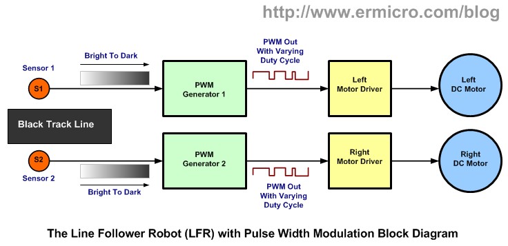
flash back theory

The LM324 Quad Op-Amp Line Follower Robot with Pulse Width Modulation

Designing a simple and yet functional Line Follower Robot (LFR) is always a fascinating and challenging subject to be learned, the LFR actually could be implemented in many ways start from a simple two transistors to a sophisticated PID (Proportional, Integrate and Differential) which take advantage of the programmable feature of microcontroller to calculate the PID equation to successfully navigate the black track line on a white background surface.
Designing a non microcontroller based LFR is quite challenging tasks as we need to limit the electronic components numbers so the LFR will not too complicated to be built by most average robotics beginners or electronic hobbyists, but at the same time we need to have a good speed control mechanism in order for the LFR to navigate the black track line successfully. The microcontroller based design LFR in the other hand is a popular choice because it reduces a number of electronic components significantly while still providing a flexible programmable control to the LFR.

On this tutorial we are going to build yet another LFR using just the standard analog components easily found on the market but use the same speed control method technique found in many good microcontroller based Line Follower Robot design. As the result we could get a good precision analog line follower robot that comparable to the microcontroller based Line Follower Robot design. On this tutorial you will also learn many useful information of how to use the operational amplifier.
The Line Follower Robot
This Line Follower Robot basically use a Cadmium Sulphide (CdS) photocell sensor or known as Light Dependent Resistor (LDR) and the high intensity blue Light Emitting Diode (LED) to illuminate the area under the photocell sensor to sense the black track line and the DC motor speed control technique to navigate the black line track as shown on this following picture:

The easy method to navigate the black track line is to turn ON and OFF the left or the right DC motor according to the sensor reading (black turn OFF and white turn ON), but using this method will make the LFR to move in zigzag way. By proportionally control both left and right DC motor speed according to the light intensity level received by the photocell sensor (reflected back by the black track line) we could make the LFR easily navigate this track. The common technique to control the motor speed efficiently is to use a pulse signal known as the pulse width modulation or PWM for short.

PWM basically is an ON and OFF pulse signal with a constant period or frequency. The proportion of pulse ON time to the pulse period is called a “duty cycle” and it expressed in percentage. For example if the proportion of pulse ON time is 50% to the total pulse period than we say that the PWM duty cycle is 50%. The PWM duty cycle percentage is corresponding to the average power produced by the pulse signal; the lower percentage produces less power than the higher percentage.
Therefore by changing the PWM duty cycles we could change the average voltage across the DC motor terminals, this mean we could vary the DC motor speed just by changing the PWM duty cycle. Therefore to make the LFR smoothly navigate the black track line, we have to adjust the PWM duty cycle according to the photocell sensor reading. The brighter light intensity level received by sensor (sensor is on the white surface) will result in higher PWM duty cycle percentage and the darker light intensity level (sensor is on the black line) received by photocell sensor will result in lower PWM duty cycle percentage.

By converting each of the photocell sensor light intensity level reading to the corresponding voltage level we could achieve this objective by using what is known as the Voltage Control Pulse Width Modulation principal.
Actually generating the PWM signal is easier with microcontroller instead of discrete components because all you have to do is to program the microcontroller PWM peripheral to do the task. On this tutorial we will learn of how to build this LFR with Voltage Control PWM using the same working principal found in many today’s modern microcontroller but using just the analog electronic components.
Now let list down the necessary electronic and other supported components to build this awesome LFR:
1. Resistors: 220 (2), 1K (2), 15K (1), 33K (1), 47K (2), and 100K (1)
2. Trimpots: 100K (2)
3. Two Light Dependent Resistor (dark above 100KOhm and below 5KOhm on bright light intensity)
4. Capacitors: 47uF/16v (1) and 0.1uF (5)
5. Diodes: 1N4148 (2)
6. High Intensity 3 mm blue Light Emitting Diode (2)
7. Optional 5 mm auto flash RGB LED with 330 Ohm resistor for the power indicator
8. Transistors: BC639 (2)
9. IC: National Semiconductor LM324 Quad Operational Amplifier (1)
10. DC Motor: Solarbotics GM2 Geared DC motor with Wheel (2)
11. Prototype Board: 52 x 38 mm for main board and 50 x 15 mm for sensors
12. 3xAA Battery holder
13. CD/DVD ROM (2)
14. Plastic Beads and Paper Clip for the castor (the third wheel)
15. Bolt, Nuts, Double Tape and Standard Electrical Tape for the black line
The complete Line Follower Robot electronics schematic is shown on this following picture:

The Voltage Control PWM
The main brain of this Line Follower Robot is lay behind the LM324 quad operational amplifier from National Semiconductor. The dual in line LM324 packages contains four identical op-amps and is specially designed to operate as an analog device.

The voltage control PWM could be generated by first using the triangle signal generator which provide the basic PWM pulse frequency and the necessary ramp voltage (rise and down) to produce the PWM signal. Next by continuously comparing this ramp voltage according to the voltage level produced by the photocell sensor using the comparator circuit we could produced the exact voltage control PWM as shown on this following picture.

When the triangle rise ramp signal reaches the voltage threshold point it will turn ON the comparator because the comparator non inverting input (V+) voltage is greater than the comparator inverting input (V-) voltage and when the down ramp signal reaches the voltage threshold point it will turn OFF the comparator because now the comparator inverting input (V-) voltage is greater than the comparator non inverting input (V+) voltage. You could read more about how the comparator works on Working with the Comparator Circuit in this blog.
If we set the threshold point voltage higher, then the ON period will be shorten; and if we set the threshold point voltage lower, then the ON period will be longer. Therefore by varying the threshold point voltage we could also vary the ON and OFF period of the comparator which is the exact behavior that we are looking for to produce the required PWM signal to drive the Line Follower Robot geared DC motor.

The ramp signal is provided by the two op-amps (U1A and U1B) that generate the triangle wave signal while the comparator for producing the PWM to each DC motor is provided by the other two op-amps (U1C and U1D) that receipt its input from the voltage divider circuit (VR and LDR) which provide the voltage threshold point and together with the triangle wave to produce the required PWM pulse

The PWM principal explained above is also used in many today’s modern microcontrollers PWM peripheral; but instead of processing the analog signal it process the digital signal. The ramp signal is replaced by the digital counter (TIMER peripheral) that will count up from 0 to 255 and start from 0 again, while the threshold point voltage is provided by threshold point register that hold the digital value (e.g. 100).

Microcontroller uses the digital comparator to compare these two digital values, when the digital counter counting up and reach the threshold point (i.e. 100) then the PWM peripheral will turn on to the output port and when it reach the maximum value (i.e. 255) it will turn off to the output port. Therefore by changing the threshold point register value we could change the PWM duty cycle output. You could read more about microcontroller based PWM on H-Bridge Microchip PIC Microcontroller PWM Motor Controller and Introduction to AVR Microcontroller Pulse Width Modulation (PWM) articles on this blog.
When designing the electronic circuit is a good habit to prototype it first, the prototype circuit enables us to fine tune the electronics design and give us the picture (signal wave) of how the circuit really works. The following picture is the Line Follower Robot circuit prototype on a breadboard complete with sensor (LED and LDR pairs) and the GM2 geared DC motor from Solarbotics.

The Triangle Wave Generator Circuit
Now as you understand the principal of how the Line Follower Circuit works than let’s take a look at the triangle wave generator circuit. In order to make it easy to understand I redraw the electronic schematic circuit separately as shown on this following picture:

To generate the triangle wave we need to use the Schmitt Trigger circuit (also called a comparator with hysteresis) that act as ON and OFF switch to the Integrator circuit input. The integrator uses the R5 and C2 to produce the necessary triangle linear ramp (up and down) on its output.
When the power up we assume the U1A output is HIGH (Vcc); the C2 capacitor will start to charge through the R5 resistor. Because the R5 and C2 is connected to the U1B inverting input (V-), therefore the U1B output will start to ramp down. The U1A non inverting input (V+) get the positive feedback from R3 and R4, when the U1B output voltage reach the threshold voltage below Vref than it will turn the U1A output to LOW (0). This bottom threshold voltage could be calculated as follow:
Vth = (R4 (Vout-u1a – Vout-u1b) / (R4 + R3)) + Vou-u1b; Vout-u1a = Vcc; Vcc = 4.5 Volt
Vth <= Vref, Vref = 0.4 Vcc
(R4 (Vcc – Vout-u1b) / (R4 + R3)) + Vout-u1b <= 0.4 Vcc
Now putting all the resistors value then we will get this following result:
(47 (Vcc – Vout-u1b)/ 147) + Vout-u1b <= 0.4 Vcc
1.4 – 0.3 Vout-u1b + Vout-u1b <= 1.8
Vout-u1b <= 0.6 Volt
Therefore the U1B output will ramp down to about 0.6 volt than the U1A output will turn OFF. Next the C2 capacitor will discharge through R5 and the UA1B output will start to ramp up and it start to increase the voltage across the R4 (Vth – threshold voltage) until the Vth voltage above the Vref voltage then the U1A output will turn to HIGH and the whole cycle will repeat again. This upper threshold voltage could be calculated as follow:
Vth = (R4 (Vout-u1a – Vout-u1b) / (R4 + R3)) + Vou-u1b; Vout-u1a = 0; Vcc = 4.5 Volt
Vth >= Vref; Vref = 0.4 Vcc
(R4 (- Vout-u1b) / (R4 + R3)) + Vout-u1b >= 0.4 Vcc
Now putting all the resistors value then we will get this following result:
(47 (- Vout-u1b)/ 147) + Vout-u1b >= 0.4 Vcc
– 0.3 Vout-u1b + Vout-u1b >= 1.8
Vout-u1b >= 2.6 Volt
Therefore the triangle voltage will ramp up from 0.6 volt to 2.6 volt then ramp down to 0.6 volt repeatedly. The frequency of the triangle wave could be calculated as follow:
Frequency = (1 / (4 x R5 x C2)) x (R3/R4) Hertz
Now putting all the resistors and capacitor value then we will get this following result:
Frequency = (1 / (4 x 15,000 x 0.0000001)) x (100,000/47,000) = 354.61 Hz
As you might guess the actual frequency measured on this Line Follower Robot prototype circuit above is about 292 Hz, this is due to the electronic components tolerance value (resistors and capacitors). Therefore if you want to have the exact frequency you could put a 100K trimport in series with R5 resistors. The voltage divider R1 and R2 provide the voltage reference (DC bias voltage) to both U1A and U1B op-amps.
The Sensor Circuit
As mention above this Line Follower Robot take advantage of the photo-resistor (CdS) known as Light Dependent Resistor (LDR). The LDR will decreases its resistance in the presence of light and increase its resistance in the dark. The region under the LDR is illuminate with a high intensity blue LED, the white surface will reflect most of the light to the LDR surface while the black track line will absorb most of the light, therefore less light will reflect to the LDR surface.

As the robot move on the black track line the LDR will continuously capture the reflected light and convert this light intensity into the corresponding voltage and feeding it to the inverting input (V-) of U1C (left sensor) and U1D (right sensor).

The 100K trimpot and LDR basically is the voltage divider circuit when the LDR detect the black track line it will receive less light intensity (LDR resistance increase) and the voltage (V-) will increase; this will decrease the PWM duty cycle output and as the result the geared DC motor will turn slowly or stop. When the LDR on the white surface it will receive maximum light intensity (LDR resistance decrease) and the voltage (V-) will decrease; this will increase the PWM duty cycle output and as the result the geared DC motor will turn fast.
You could simply exchange the comparator V+ and V- input source to make the Line Follower Robot detect the white line on the black surface instead of normal black line on the white surface. By using two DPDT (Double Pole Double Throw) switches you could achieve this behavior as shown on this following picture:

The geared DC motor driver uses the BC639 transistor and the base terminal is connected to the comparator output through the 1K resistor. The transistor is operated as a switch which turns ON and OFF the geared DC motor according to the PWM pulse current it received from the comparator. The 0.1uF capacitor across the geared DC motor’s terminal is used to reduce noise generated by the DC motor. .
The Line Follower Robot Construction
The Line Follower Robot construction could be constructed freely but the easiest one is to use the discarded CD/DVD ROM as shown on this following pictures:

I glue the two CDROM together in order to make more room and attached the two DC motors, 3xAA battery holder, main board and sensor board using the double tape. The sensor sensitivities and the Line Follower Robot speed could be controlled by adjusting the 100K trimport. After putting all the parts together now is time to watch how this nice Line Follower Robot in action:

.

Samples

Development Tools

Quick Print

Buy
it now

MCP6001
DATA SHEET
(11/18/2009) DOWNLOAD

MCP6001

In Production

The MCP6001 is a single general purpose op amp offering rail-to-rail input and output over the 1.8 to 6V operating range. This amplifier has a typical GBWP of 1 MHz with typical quiescent current of 100 microamperes. The MCP6001 is available in SC-70 and SOT-23 packages.

Features

Gain Bandwidth Product (GBWP): 1 MHz
Quiescent Current: 100 µA (typ.)
Supply voltage range: 1.8V to 6V
Rail to Rail Input and Output
Extended Temperature Range
Space Saving Package Offering: SC70, SOT23

Parameter Name

Value

Temp. Range (°C)

-40°C to +125°C

Vos Max (µV)

4500

# per Package

Iq Typical (µA)

100

Iq Max (µA)

170

GBWP (kHz)

1000

Operating Voltage Range (V)

1.8 to 6.0

Device Description

Linear Op Amps

Input Voltage Noise Density (nV/rt(Hz))

PSRR Min (dB)

CMRR Min (dB)

Vos/Ta (uV/°C)

Ib (pA)

Aol (dB)

112

PM (deg)

Isc (mA)

Rail-to-Rail

In/Out

Unity Gain Stable

Yes

Slew Rate V/uS

0.6

GO LOOK IMPORTANTBOOK

Rabu, 23 Agustus 2017

Transistor upgrade system to operational amplifier and then At a glance Developing a flying car o Auto Mobile AMNIMARJESLOW GOVERNMENT GOOD JOB GOOD COLLABORATION ON MA THE MATIC 222 2049 91220017

Introduction

Basic Theory

Layout Considerations

Microprocessor Control

Scalable electronics driving autonomous vehicle technologies

Operational Amplifiers (Op Amps)

A Collection of Amp Applications

MCP6001

In Production

Features

Tidak ada komentar:

Posting Komentar

Pengikut

Cari Blog Ini

Cari Blog Ini

Translate