High fidelity—or hi-fi or hifi—reproduction is a term used by home stereo listeners, audiophiles and home audio enthusiasts to refer to high-quality reproduction of sound to distinguish it from the lower quality sound produced by inexpensive audio equipment, or the inferior quality of sound reproduction that can be heard in recordings made until the late 1940s.
Ideally, high-fidelity equipment has inaudible noise and distortion, and a flat (neutral, uncolored) frequency response within the intended frequency range.

Hi-fi speakers are a key component of quality audio reproduction.

bright cloud

Bell Laboratories began experimenting with a wider range of recording techniques in the early 1930s. Performances by Leopold Stokowski and the Philadelphia Orchestra were recorded in 1931 and 1932 using telephone lines between the Academy of Music in Philadelphia and the Bell labs in New Jersey. Some multitrack recordings were made on optical sound film, which led to new advances used primarily by MGM (as early as 1937) and 20th Century-Fox Film Corporation (as early as 1941). RCA Victor began recording performances by several orchestras using optical sound around 1941, resulting in higher-fidelity masters for 78-rpm discs. During the 1930s, Avery Fisher, an amateur violinist, began experimenting with audio design and acoustics. He wanted to make a radio that would sound like he was listening to a live orchestra—that would achieve high fidelity to the original sound. After World War II, Harry F. Olson conducted an experiment whereby test subjects listened to a live orchestra through a hidden variable acoustic filter. The results proved that listeners preferred high fidelity reproduction, once the noise and distortion introduced by early sound equipment was removed.
Beginning in 1948, several innovations created the conditions that made for major improvements of home-audio quality possible:

Reel-to-reel audio tape recording, based on technology taken from Germany after WWII, helped musical artists such as Bing Crosby make and distribute recordings with better fidelity.
The advent of the 33⅓ rpm Long Play (LP) microgroove vinyl record, with lower surface noise and quantitatively specified equalization curves as well as noise-reduction and dynamic range systems. Classical music fans, who were opinion leaders in the audio market, quickly adopted LPs because, unlike with older records, most classical works would fit on a single LP.
FM radio, with wider audio bandwidth and less susceptibility to signal interference and fading than AM radio, though AM could be heard at longer distances at night.
Better amplifier designs, with more attention to frequency response and much higher power output capability, reproducing audio without perceptible distortion.
New loudspeaker designs, including acoustic suspension, developed by Edgar Villchur and Henry Kloss improved bass frequency response.

In the 1950s, audio manufacturers employed the phrase high fidelity as a marketing term to describe records and equipment intended to provide faithful sound reproduction. While some consumers simply interpreted high fidelity as fancy and expensive equipment, many found the difference in quality between "hi-fi" and the then standard AM radios and 78 rpm records readily apparent and bought 33⅓ LPs such as RCA's New Orthophonics and London's ffrr (Full Frequency Range Recording, a UK Decca system); and high-fidelity phonographs. Audiophiles paid attention to technical characteristics and bought individual components, such as separate turntables, radio tuners, preamplifiers, power amplifiers and loudspeakers. Some enthusiasts even assembled their own loudspeaker systems. In the 1950s, hi-fi became a generic term for home sound equipment, to some extent displacing phonograph and record player.
In the late 1950s and early 1960s, the development of the Westrex single-groove stereophonic record cutterhead led to the next wave of home-audio improvement, and in common parlance, stereo displaced hi-fi. Records were now played on a stereo. In the world of the audiophile, however, the concept of high fidelity continued to refer to the goal of highly accurate sound reproduction and to the technological resources available for approaching that goal. This period is regarded as the "Golden Age of Hi-Fi", when vacuum tube equipment manufacturers of the time produced many models considered endearing by modern audiophiles, and just before solid state (transistorized) equipment was introduced to the market, subsequently replacing tube equipment as the mainstream technology.
A popular type of system for reproducing music beginning in the 1970s was the integrated music centre—which combined a phonograph turntable, AM-FM radio tuner, tape player, preamplifier, and power amplifier in one package, often sold with its own separate, detachable or integrated speakers. These systems advertised their simplicity. The consumer did not have to select and assemble individual components, or be familiar with impedance and power ratings. Purists generally avoid referring to these systems as high fidelity, though some are capable of very good quality sound reproduction. Audiophiles in the 1970s and 1980s preferred to buy each component separately. That way, they could choose models of each component with the specifications that they desired. In the 1980s, a number of audiophile magazines became available, offering reviews of components and articles on how to choose and test speakers, amplifiers and other components.

Listening tests

Listening tests are used by hi-fi manufacturers, audiophile magazines and audio engineering researchers and scientists. If a listening test is done in such a way that the listener who is assessing the sound quality of a component or recording can see the components that are being used for the test (e.g., the same musical piece listened to through a tube power amplifier and a solid state amplifier), then it is possible that the listener's pre-existing biases towards or against certain components or brands could affect their judgement. To respond to this issue, researchers began to use blind tests, in which the researchers can see the components being tested, but not the listeners undergoing the experiments. In a double-blind experiment, neither the listeners nor the researchers know who belongs to the control group and the experimental group, or which type of audio component is being used for which listening sample. Only after all the data has been recorded (and in some cases, analyzed) do the researchers learn which components or recordings were preferred by the listeners. A commonly used variant of this test is the ABX test. A subject is presented with two known samples (sample A, the reference, and sample B, an alternative), and one unknown sample X, for three samples total. X is randomly selected from A and B, and the subject identifies X as being either A or B. Although there is no way to prove that a certain lossy methodology is transparent, a properly conducted double-blind test can prove that a lossy method is not transparent.
Scientific double-blind tests are sometimes used as part of attempts to ascertain whether certain audio components (such as expensive, exotic cables) have any subjectively perceivable effect on sound quality. Data gleaned from these double-blind tests is not accepted by some "audiophile" magazines such as Stereophile and The Absolute Sound in their evaluations of audio equipment. John Atkinson, current editor of Stereophile, stated (in a 2005 July editorial named Blind Tests & Bus Stops) that he once purchased a solid-state amplifier, the Quad 405, in 1978 after seeing the results from blind tests, but came to realize months later that "the magic was gone" until he replaced it with a tube amp. Robert Harley of The Absolute Sound wrote, in a 2008 editorial (on Issue 183), that: "...blind listening tests fundamentally distort the listening process and are worthless in determining the audibility of a certain phenomenon."
Doug Schneider, editor of the online Soundstage network, refuted this position with two editorials in 2009. He stated: "Blind tests are at the core of the decades’ worth of research into loudspeaker design done at Canada’s National Research Council (NRC). The NRC researchers knew that for their result to be credible within the scientific community and to have the most meaningful results, they had to eliminate bias, and blind testing was the only way to do so." Many Canadian companies such as Axiom, Energy, Mirage, Paradigm, PSB and Revel use blind testing extensively in designing their loudspeakers. Audio professional Dr. Sean Olive of Harman International shares this view.

Semblance of realism

Stereophonic sound provided a partial solution to the problem of creating the illusion of live orchestral performers by creating a phantom middle channel when the listener sits exactly in the middle of the two front loudspeakers. When the listener moves slightly to the side, however, this phantom channel disappears or is greatly reduced. An attempt to provide for the reproduction of the reverberation was tried in the 1970s through quadraphonic sound but, again, the technology at that time was insufficient for the task. Consumers did not want to pay the additional costs and space required for the marginal improvements in realism. With the rise in popularity of home theater, however, multi-channel playback systems became affordable, and many consumers were willing to tolerate the six to eight channels required in a home theater. The advances made in signal processors to synthesize an approximation of a good concert hall can now provide a somewhat more realistic illusion of listening in a concert hall.
In addition to spatial realism, the playback of music must be subjectively free from noise, such as hiss or hum, to achieve realism. The compact disc (CD) provides about 90 decibels of dynamic range, which exceeds the 80 dB dynamic range of music as normally perceived in a concert hall. Audio equipment must be able to reproduce frequencies high enough and low enough to be realistic. The human hearing range, for healthy young persons, is 20 Hz to 20,000 Hz. Most adults can't hear higher than 15 kHz. CDs are capable of reproducing frequencies as low as 10 Hz and as high as 22.05 kHz, making them adequate for reproducing the frequency range that most humans can hear. The equipment must also provide no noticeable distortion of the signal or emphasis or de-emphasis of any frequency in this frequency range.

Modularity

Modular components made by Samsung and Harman Kardon

Integrated, mini, or lifestyle systems, also known as music centres or minisystems, contain one or more sources such as a CD player, a tuner, or a cassette deck together with a preamplifier and a power amplifier in one box. Although some high-end manufacturers do produce integrated systems, such products are generally disparaged by audiophiles, who prefer to build a system from separates (or components), often with each item from a different manufacturer specialising in a particular component. This provides the most flexibility for piece-by-piece upgrades and repairs.
For slightly less flexibility in upgrades, a preamplifier and a power amplifier in one box is called an integrated amplifier; with a tuner, it is a receiver. A monophonic power amplifier, which is called a monoblock, is often used for powering a subwoofer. Other modules in the system may include components like cartridges, tonearms, hi-fi turntables, Digital Media Players, digital audio players, DVD players that play a wide variety of discs including CDs, CD recorders, MiniDisc recorders, hi-fi videocassette recorders (VCRs) and reel-to-reel tape recorders. Signal modification equipment can include equalizers and signal processors.
This modularity allows the enthusiast to spend as little or as much as they want on a component that suits their specific needs. In a system built from separates, sometimes a failure on one component still allows partial use of the rest of the system. A repair of an integrated system, though, means complete lack of use of the system. Another advantage of modularity is the ability to spend money on only a few core components at first and then later add additional components to the system. Some of the disadvantages of this approach are increased cost, complexity, and space required for the components.

Modern equipment

In the 2000s, modern hi-fi equipment can include signal sources such as digital audio tape (DAT), digital audio broadcasting (DAB) or HD Radio tuners. Some modern hi-fi equipment can be digitally connected using fibre optic TOSLINK cables, universal serial bus (USB) ports (including one to play digital audio files), or Wi-Fi support. Another modern component is the music server consisting of one or more computer hard drives that hold music in the form of computer files. When the music is stored in an audio file format that is lossless such as FLAC, Monkey's Audio or WMA Lossless, the computer playback of recorded audio can serve as an audiophile-quality source for a hi-fi system.

X . I

Sound recording and reproduction

Sound recording and reproduction is an electrical, mechanical, electronic, or digital inscription and re-creation of sound waves, such as spoken voice, singing, instrumental music, or sound effects. The two main classes of sound recording technology are analog recording and digital recording.
Acoustic analog recording is achieved by a microphone diaphragm that can detect and sense the changes in atmospheric pressure caused by acoustic sound waves and record them as a mechanical representation of the sound waves on a medium such as a phonograph record (in which a stylus cuts grooves on a record). In magnetic tape recording, the sound waves vibrate the microphone diaphragm and are converted into a varying electric current, which is then converted to a varying magnetic field by an electromagnet, which makes a representation of the sound as magnetized areas on a plastic tape with a magnetic coating on it. Analog sound reproduction is the reverse process, with a bigger loudspeaker diaphragm causing changes to atmospheric pressure to form acoustic sound waves. Oscillations may also be recorded directly from devices such as an electric guitar pickup or a synthesizer, without the use of acoustics in the recording process, other than the need for musicians to hear how well they are playing during recording sessions via headphones.
Digital recording and reproduction converts the analog sound signal picked up by the microphone to a digital form by the process of digitization. This lets the audio data be stored and transmitted by a wider variety of media. Digital recording stores audio as a series of binary numbers (zeros and ones) representing samples of the amplitude of the audio signal at equal time intervals, at a sample rate high enough to convey all sounds capable of being heard. Digital recordings are considered higher quality than analog recordings not necessarily because they have higher fidelity (wider frequency response or dynamic range), but because the digital format can prevent much loss of quality found in analog recording due to noise and electromagnetic interference in playback and mechanical deterioration or damage to the storage medium. Whereas successive copies of an analog recording tend to degrade in quality, as more noise is added, a digital audio recording can be reproduced endlessly with no degradation in sound quality. A digital audio signal must be reconverted to analog form during playback before it is amplified and connected to a loudspeaker to produce sound.

bright cloud

Long before sound was first recorded, music was recorded—first by written notation, then also by mechanical devices (e.g., wind-up music boxes, in which a mechanism turns a spindle, which plucks tines, thus producing a melody). Automatic music reproduction traces back as far as the 9th century, when the Banū Mūsā brothers invented the earliest known mechanical musical instrument, in this case, a hydropowered organ that played interchangeable cylinders. According to Charles B. Fowler, this "...cylinder with raised pins on the surface remained the basic device to produce and reproduce music mechanically until the second half of the nineteenth century." The Banu Musa brothers also invented an automatic flute player, which appears to have been the first programmable machine. According to Fowler, the automata were a robot band that performed "...more than fifty facial and body actions during each musical selection." In the 14th century, Flanders introduced a mechanical bell-ringer controlled by a rotating cylinder. Similar designs appeared in barrel organs (15th century), musical clocks (1598), barrel pianos (1805), and musical boxes (ca.1800).
The fairground organ, developed in 1892, used a system of accordion-folded punched cardboard books. The player piano, first demonstrated in 1876, used a punched paper scroll that could store an arbitrarily long piece of music. The most sophisticated of the piano rolls were "hand-played", meaning that the roll represented the actual performance of an individual, not just a transcription of the sheet music. This technology to record a live performance onto a piano roll was not developed until 1904. Piano rolls were in continuous mass production from 1896 to 2008. A 1908 U.S. Supreme Court copyright case noted that, in 1902 alone, there were between 70,000 and 75,000 player pianos manufactured, and between 1,000,000 and 1,500,000 piano rolls produced. The use of piano rolls began to decline in the 1920s although one type is still being made today.

Phonautograph

The first device that could record actual sounds as they passed through the air (but could not play them back—the purpose was only visual study) was the phonautograph, patented in 1857 by Parisian inventor Édouard-Léon Scott de Martinville. The earliest known recordings of the human voice are phonautograph recordings, called "phonautograms", made in 1857. They consist of sheets of paper with sound-wave-modulated white lines created by a vibrating stylus that cut through a coating of soot as the paper was passed under it. An 1860 phonautogram of Au Clair de la Lune, a French folk song, was played back as sound for the first time in 2008 by scanning it and using software to convert the undulating line, which graphically encoded the sound, into a corresponding digital audio file.

Phonograph

Phonograph cylinder

0:00

On April 30, 1877, French poet, humorous writer and inventor Charles Cros submitted a sealed envelope containing a letter to the Academy of Sciences in Paris fully explaining his proposed method, called the paleophone. Though no trace of a working paleophone was ever found, Cros is remembered as the earliest inventor of a sound recording and reproduction machine. The first practical sound recording and reproduction device was the mechanical phonograph cylinder, invented by Thomas Edison in 1877 and patented in 1878. The invention soon spread across the globe and over the next two decades the commercial recording, distribution, and sale of sound recordings became a growing new international industry, with the most popular titles selling millions of units by the early 1900s. The development of mass-production techniques enabled cylinder recordings to become a major new consumer item in industrial countries and the cylinder was the main consumer format from the late 1880s until around 1910.

Disc phonograph

0:00

Recording of Bell's voice on a wax disc in 1885, identified in 2013

Emile Berliner with disc record gramophone

The next major technical development was the invention of the gramophone disc, generally credited to Emile Berliner and commercially introduced in the United States in 1889, though others had demonstrated similar disk apparatus earlier, most notably Alexander Graham Bell in 1881. Discs were easier to manufacture, transport and store, and they had the additional benefit of being louder (marginally) than cylinders, which by necessity, were single-sided. Sales of the gramophone record overtook the cylinder ca. 1910, and by the end of World War I the disc had become the dominant commercial recording format. Edison, who was the main producer of cylinders, created the Edison Disc Record in an attempt to regain his market. In various permutations, the audio disc format became the primary medium for consumer sound recordings until the end of the 20th century, and the double-sided 78 rpm shellac disc was the standard consumer music format from the early 1910s to the late 1950s.
Although there was no universally accepted speed, and various companies offered discs that played at several different speeds, the major recording companies eventually settled on a de facto industry standard of nominally 78 revolutions per minute, though the actual speed differed between America and the rest of the world. The specified speed was 78.26 rpm in America and 77.92 rpm throughout the rest of the world, the difference in speeds was a result of the difference in cycle frequencies of the AC power driving the stroboscopes used to calibrate recording lathes and turntables. The nominal speed of the disc format gave rise to its common nickname, the "seventy-eight" (though not until other speeds had become available). Discs were made of shellac or similar brittle plastic-like materials, played with needles made from a variety of materials including mild steel, thorn, and even sapphire. Discs had a distinctly limited playing life that varied depending on how they were produced.
Earlier, purely acoustic methods of recording had limited sensitivity and frequency range. Mid-frequency range notes could be recorded, but very low and very high frequencies could not. Instruments such as the violin were difficult to transfer to disc. One technique to deal with this involved using a Stroh violin—which was fitted a conical horn connected to a diaphragm vibrated by the violin bridge. The horn was no longer required once electrical recording was developed.
The long-playing 33 ¹⁄₃ rpm microgroove vinyl record, or "LP", was developed at Columbia Records and introduced in 1948. The short-playing but convenient 7-inch 45 rpm microgroove vinyl single was introduced by RCA Victor in 1949. In the US and most developed countries, the two new vinyl formats completely replaced 78 rpm shellac discs by the end of the 1950s, but in some corners of the world, the "78" lingered on far into the 1960s. Vinyl was much more expensive than shellac, one of several factors that made its use for 78 rpm records very unusual, but with a long-playing disc the added cost was acceptable and the compact "45" format required very little material. Vinyl offered improved performance, both in stamping and in playback. If played with a good diamond stylus mounted in a lightweight pickup on a well-adjusted tonearm, it was long-lasting. If protected from dust, scuffs and scratches there was very little noise. Vinyl records were, over-optimistically, advertised as "unbreakable". They were not, but they were much less fragile than shellac, which had itself once been touted as "unbreakable" compared to wax cylinders.

Electrical recording

RCA-44, a classic ribbon microphone introduced in 1932. Similar units were widely used for recording and broadcasting in the 1940s and are occasionally still used today.

Between the invention of the phonograph in 1877 and the first commercial digital recordings in the early 1970s, arguably the most important milestone in the history of sound recording was the introduction of what was then called electrical recording, in which a microphone was used to convert the sound into an electrical signal that was amplified and used to actuate the recording stylus. This innovation eliminated the "horn sound" resonances characteristic of the acoustical process, produced clearer and more full-bodied recordings by greatly extending the useful range of audio frequencies, and allowed previously unrecordable distant and feeble sounds to be captured.
Sound recording began as a purely mechanical process. Except for a few crude telephone-based recording devices with no means of amplification, such as the Telegraphone, it remained so until the 1920s when several radio-related developments in electronics converged to revolutionize the recording process. These included improved microphones and auxiliary devices such as electronic filters, all dependent on electronic amplification to be of practical use in recording. In 1906, Lee De Forest invented the Audion triode vacuum tube, an electronic valve that could amplify weak electrical signals. By 1915, it was in use in long-distance telephone circuits that made conversations between New York and San Francisco practical. Refined versions of this tube were the basis of all electronic sound systems until the commercial introduction of the first transistor-based audio devices in the mid-1950s.
During World War I, engineers in the United States and Great Britain worked on ways to record and reproduce, among other things, the sound of a German U-boat for training purposes. Acoustical recording methods of the time could not reproduce the sounds accurately. The earliest results were not promising.
The first electrical recording issued to the public, with little fanfare, was of November 11, 1920, funeral services for The Unknown Warrior in Westminster Abbey, London. The recording engineers used microphones of the type used in contemporary telephones. Four were discreetly set up in the abbey and wired to recording equipment in a vehicle outside. Although electronic amplification was used, the audio was weak and unclear. The procedure did, however, produce a recording that would otherwise not have been possible in those circumstances. For several years, this little-noted disc remained the only issued electrical recording.
Several record companies and independent inventors, notably Orlando Marsh, experimented with equipment and techniques for electrical recording in the early 1920s. Marsh's electrically recorded Autograph Records were already being sold to the public in 1924, a year before the first such offerings from the major record companies, but their overall sound quality was too low to demonstrate any obvious advantage over traditional acoustical methods. Marsh's microphone technique was idiosyncratic and his work had little if any impact on the systems being developed by others.
Telephone industry giant Western Electric had research laboratories (merged with the AT&T engineering department in 1925 to form Bell Telephone Laboratories) with material and human resources that no record company or independent inventor could match. They had the best microphone, a condenser type developed there in 1916 and greatly improved in 1922, and the best amplifiers and test equipment. They had already patented an electromechanical recorder in 1918, and in the early 1920s, they decided to intensively apply their hardware and expertise to developing two state-of-the-art systems for electronically recording and reproducing sound: one that employed conventional discs and another that recorded optically on motion picture film. Their engineers pioneered the use of mechanical analogs of electrical circuits and developed a superior "rubber line" recorder for cutting the groove into the wax master in the disc recording system.
By 1924, such dramatic progress had been made that Western Electric arranged a demonstration for the two leading record companies, the Victor Talking Machine Company and the Columbia Phonograph Company. Both soon licensed the system and both made their earliest published electrical recordings in February 1925, but neither actually released them until several months later. To avoid making their existing catalogs instantly obsolete, the two long-time archrivals agreed privately not to publicize the new process until November 1925, by which time enough electrically recorded repertory would be available to meet the anticipated demand. During the next few years, the lesser record companies licensed or developed other electrical recording systems. By 1929 only the budget label Harmony was still issuing new recordings made by the old acoustical process.
Comparison of some surviving Western Electric test recordings with early commercial releases indicates that the record companies "dumbed down" the frequency range of the system so the recordings would not overwhelm non-electronic playback equipment, which reproduced very low frequencies as an unpleasant rattle and rapidly wore out discs with strongly recorded high frequencies.

Other recording formats

In the 1920s, Phonofilm and other early motion picture sound systems employed optical recording technology, in which the audio signal was graphically recorded on photographic film. The amplitude variations comprising the signal were used to modulate a light source which was imaged onto the moving film through a narrow slit, allowing the signal to be photographed as variations in the density or width of a "sound track". The projector used a steady light and a photoelectric cell to convert these variations back into an electrical signal, which was amplified and sent to loudspeakers behind the screen. Ironically, the introduction of "talkies" was spearheaded by The Jazz Singer (1927), which used the Vitaphone sound-on-disc system rather than an optical soundtrack. Optical sound became the standard motion picture audio system throughout the world and remains so for theatrical release prints despite attempts in the 1950s to substitute magnetic soundtracks. Currently, all release prints on 35 mm film include an analog optical soundtrack, usually stereo with Dolby SR noise reduction. In addition, an optically recorded digital soundtrack in Dolby Digital and/or Sony SDDS form is likely to be present. An optically recorded timecode is also commonly included to synchronise CDROMs that contain a DTS soundtrack.
This period also saw several other historic developments including the introduction of the first practical magnetic sound recording system, the magnetic wire recorder, which was based on the work of Danish inventor Valdemar Poulsen. Magnetic wire recorders were effective, but the sound quality was poor, so between the wars, they were primarily used for voice recording and marketed as business dictating machines. In 1924, a German engineer, Dr. Kurt Stille, developed the Poulsen wire recorder as a dictating machine. The following year, Ludwig Blattner began work that eventually produced the Blattnerphone,enhancing it to use steel tape instead of wire. The BBC started using Blattnerphones in 1930 to record radio programmes. In 1933, radio pioneer Guglielmo Marconi's company purchased the rights to the Blattnerphone, and newly developed Marconi-Stille recorders were installed in the BBC's Maida Vale Studios in March 1935. The tape used in Blattnerphones and Marconi-Stille recorders was the same material used to make razor blades, and not surprisingly the fearsome Marconi-Stille recorders were considered so dangerous that technicians had to operate them from another room for safety. Because of the high recording speeds required, they used enormous reels about one metre in diameter, and the thin tape frequently broke, sending jagged lengths of razor steel flying around the studio. The K1 Magnetophon was the first practical tape recorder, developed by AEG in Germany in 1935.

Magnetic tape

Magnetic tape sound recording

Magnetic audio tapes: acetate base (left) and polyester base (right)

An important field of invention during this period was the tape recorder. Magnetic tape recording uses an amplified electrical audio signal to generate analogous variations of the magnetic field produced by a tape head, which impresses corresponding variations of magnetization on the moving tape. In playback mode, the signal path is reversed, the tape head acting as a miniature electric generator as the varyingly magnetized tape passes over it. The original solid steel ribbon was replaced by a much more practical coated paper tape, but acetate soon replaced paper as the standard tape base. Acetate has fairly low tensile strength and if very thin it will snap easily, so it was in turn eventually superseded by polyester. This technology, the basis for almost all commercial recording from the 1950s to the 1980s, was developed in the 1930s by German audio engineers who also rediscovered the principle of AC biasing (first used in the 1920s for wire recorders), which dramatically improved the frequency response of tape recordings. The technology was further improved just after World War II by American audio engineer John T. Mullin with backing from Bing Crosby Enterprises. Mullin's pioneering recorders were modifications of captured German recorders. In the late 1940s, the Ampex company produced the first tape recorders commercially available in the US.

A typical Compact Cassette

Magnetic tape brought about sweeping changes in both radio and the recording industry. Sound could be recorded, erased and re-recorded on the same tape many times, sounds could be duplicated from tape to tape with only minor loss of quality, and recordings could now be very precisely edited by physically cutting the tape and rejoining it. Within a few years of the introduction of the first commercial tape recorder—the Ampex 200 model, launched in 1948—American musician-inventor Les Paul had invented the first multitrack tape recorder, ushering in another technical revolution in the recording industry. Tape made possible the first sound recordings totally created by electronic means, opening the way for the bold sonic experiments of the Musique Concrète school and avant garde composers like Karlheinz Stockhausen, which in turn led to the innovative pop music recordings of artists such as Frank Zappa, The Beatles, and The Beach Boys.
The ease and accuracy of tape editing, as compared to the cumbersome disc-to-disc editing procedures previously in some limited use, together with tape's consistently high audio quality finally convinced radio networks to routinely prerecord their entertainment programming, most of which had formerly been broadcast live. Also, for the first time, broadcasters, regulators and other interested parties were able to undertake comprehensive audio logging of each day's radio broadcasts. Innovations like multitracking and tape echo allowed radio programs and advertisements to be produced to a high level of complexity and sophistication. The combined impact with innovations such as the endless loop broadcast cartridge led to significant changes in the pacing and production style of radio program content and advertising.

Stereo and hi-fi

Stereophonic sound and High fidelity

In 1881, it was noted during experiments in transmitting sound from the Paris Opera that it was possible to follow the movement of singers on the stage if earpieces connected to different microphones were held to the two ears. This discovery was commercialized in 1890 with the Théâtrophone system, which operated for over forty years until 1932. In 1931, Alan Blumlein, a British electronics engineer working for EMI, designed a way to make the sound of an actor in a film follow his movement across the screen. In December 1931, he submitted a patent including the idea, and in 1933 this became UK patent number 394,325. Over the next two years, Blumlein developed stereo microphones and a stereo disc-cutting head, and recorded a number of short films with stereo soundtracks.
In the 1930s, experiments with magnetic tape enabled the development of the first practical commercial sound systems that could record and reproduce high-fidelity stereophonic sound. The experiments with stereo during the 1930s and 1940s were hampered by problems with synchronization. A major breakthrough in practical stereo sound was made by Bell Laboratories, who in 1937 demonstrated a practical system of two-channel stereo, using dual optical sound tracks on film. Major movie studios quickly developed three-track and four-track sound systems, and the first stereo sound recording for a commercial film was made by Judy Garland for the MGM movie Listen, Darling in 1938. The first commercially released movie with a stereo soundtrack was Walt Disney's Fantasia, released in 1940. The 1941 release of Fantasia used the "Fantasound" sound system. This system used a separate film for the sound, synchronized with the film carrying the picture. The sound film had four double-width optical soundtracks, three for left, center, and right audio—and a fourth as a "control" track with three recorded tones that controlled the playback volume of the three audio channels. Because of the complex equipment this system required, Disney exhibited the movie as a roadshow, and only in the United States. Regular releases of the movie used standard mono optical 35 mm stock until 1956, when Disney released the film with a stereo soundtrack that used the "Cinemascope" four-track magnetic sound system.
German audio engineers working on magnetic tape developed stereo recording by 1941, even though a 2-track push-pull monaural technique existed in 1939. Of 250 stereophonic recordings made during WW2, only three survive: Beethoven's 5th Piano Concerto with Walter Gieseking and Arthur Rother, a Brahm's Serenade, and the last movement of Bruckner's 8th Symphony with Von Karajan. The Audio Engineering Society has issued all these recordings on CD. (Varese Sarabande had released the Beethoven Concerto on LP, and it has been reissued on CD several times since). Other early German stereophonic tapes are believed to have been destroyed in bombings. Not until Ampex introduced the first commercial two-track tape recorders in the late 1940s did stereo tape recording become commercially feasible. However, despite the availability of multitrack tape, stereo did not become the standard system for commercial music recording for some years, and remained a specialist market during the 1950s. EMI (UK) was the first company to release commercial stereophonic tapes. They issued their first Stereosonic tape in 1954. Others quickly followed, under the His Master's Voice and Columbia labels. 161 Stereosonic tapes were released, mostly classical music or lyric recordings. RCA imported these tapes into the USA.
Two-track stereophonic tapes were more successful in America during the second half of the 1950s. They were duplicated at real time (1:1) or at twice the normal speed (2:1) when later 4-track tapes were often duplicated at up to 16 times the normal speed, providing a lower sound quality in many cases. Early American 2-track stereophonic tapes were very expensive. A typical example is the price list of the Sonotape/Westminster reels: $6.95, $11.95 and $17.95 for the 7000, 9000 and 8000 series respectively. Some HMV tapes released in the USA also cost up to $15. The history of stereo recording changed after the late 1957 introduction of the Westrex stereo phonograph disc, which used the groove format developed earlier by Blumlein. Decca Records in England came out with FFRR (Full Frequency Range Recording) in the 1940s, which became internationally accepted as a worldwide standard for higher quality recording on vinyl records. The Ernest Ansermet recording of Igor Stravinsky's Petrushka was key in the development of full frequency range records and alerting the listening public to high fidelity in 1946.
Record companies mixed most popular music singles into monophonic sound until the mid-1960s—then commonly released major recordings in both mono and stereo until the early 1970s. Many 1960s pop albums available only in stereo in the 2000s were originally released only in mono, and record companies produced the "stereo" versions of these albums by simply separating the two tracks of the master tape, creating "pseudo stereo". In the mid Sixties, as stereo became more popular, many mono recordings (such as The Beach Boys' Pet Sounds) were remastered using the so-called "fake stereo" method, which spread the sound across the stereo field by directing higher-frequency sound into one channel and lower-frequency sounds into the other.

1950s to 1980s

Magnetic tape transformed the recording industry. By the early 1950s, most commercial recordings were mastered on tape instead of recorded directly to disc. Tape facilitated a degree of manipulation in the recording process that was impractical with mixes and multiple generations of directly recorded discs. An early example is Les Paul's 1951 recording of How High the Moon, on which Paul played eight overdubbed guitar tracks. In the 1960s Brian Wilson of The Beach Boys, Frank Zappa, and The Beatles (with producer George Martin) were among the first popular artists to explore the possibilities of multitrack recording techniques and effects on their landmark albums Pet Sounds, Freak Out!, and Sgt. Pepper's Lonely Hearts Club Band.
The next important innovation was small cartridge-based tape systems, of which the compact cassette, commercialized by the Philips electronics company in 1964, is the best known. Initially, a low-fidelity format for spoken-word voice recording and inadequate for music reproduction, after a series of improvements it entirely replaced the competing formats, the larger 8-track tape (used primarily in cars) and the fairly similar "Deutsche Cassette" developed by the German company Grundig. This latter system was not particularly common in Europe and practically unheard-of in America. The compact cassette became a major consumer audio format and advances in electronic and mechanical miniaturization led to the development of the Sony Walkman, a pocket-sized cassette player introduced in 1979. The Walkman was the first personal music player and it gave a major boost to sales of prerecorded cassettes, which became the first widely successful release format that used a re-recordable medium: the vinyl record was a playback-only medium and commercially prerecorded tapes for reel-to-reel tape decks, which many consumers found difficult to operate, were never more than an uncommon niche market item.

A key advance in audio fidelity came with the Dolby A noise reduction system, invented by Ray Dolby and introduced into professional recording studios in 1966. It suppressed the light but sometimes quite noticeable steady background of hiss, which was the only easily audible downside of mastering on tape instead of recording directly to disc. A competing system, dbx, invented by David Blackmer, also found success in professional audio. A simpler variant of Dolby's noise reduction system, known as Dolby B, greatly improved the sound of cassette tape recordings by reducing the especially high level of hiss that resulted from the cassette's miniaturized tape format. It, and variants, also eventually found wide application in the recording and film industries. Dolby B was crucial to the popularization and commercial success of the cassette as a domestic recording and playback medium, and it became a standard feature in the booming home and car stereo market of the 1970s and beyond. The compact cassette format also benefited enormously from improvements to the tape itself as coatings with wider frequency responses and lower inherent noise were developed, often based on cobalt and chrome oxides as the magnetic material instead of the more usual iron oxide.
The multitrack audio cartridge had been in wide use in the radio industry, from the late 1950s to the 1980s, but in the 1960s the pre-recorded 8-track cartridge was launched as a consumer audio format by Bill Lear of the Lear Jet aircraft company (and although its correct name was the 'Lear Jet Cartridge', it was seldom referred to as such). Aimed particularly at the automotive market, they were the first practical, affordable car hi-fi systems, and could produce superior sound quality to the compact cassette. However the smaller size and greater durability — augmented by the ability to create home-recorded music "compilations" since 8-track recorders were rare — saw the cassette become the dominant consumer format for portable audio devices in the 1970s and 1980s.
There had been experiments with multi-channel sound for many years — usually for special musical or cultural events — but the first commercial application of the concept came in the early 1970s with the introduction of Quadraphonic sound. This spin-off development from multitrack recording used four tracks (instead of the two used in stereo) and four speakers to create a 360-degree audio field around the listener. Following the release of the first consumer 4-channel hi-fi systems, a number of popular albums were released in one of the competing four-channel formats; among the best known are Mike Oldfield's Tubular Bells and Pink Floyd's The Dark Side of the Moon. Quadraphonic sound was not a commercial success, partly because of competing and somewhat incompatible four-channel sound systems (e.g., CBS, JVC, Dynaco and others all had systems) and generally poor quality, even when played as intended on the correct equipment, of the released music. It eventually faded out in the late 1970s, although this early venture paved the way for the eventual introduction of domestic Surround Sound systems in home theatre use, which have gained enormous popularity since the introduction of the DVD. This widespread adoption has occurred despite the confusion introduced by the multitude of available surround sound standards.

Audio components

High fidelity § Modularity

The replacement of the relatively fragile thermionic valve (vacuum tube) by the smaller, lighter-weight, cooler-running, less expensive, more robust, and less power-hungry transistor also accelerated the sale of consumer high-fidelity "hi-fi" sound systems from the 1960s onward. In the 1950s, most record players were monophonic and had relatively low sound quality. Few consumers could afford high-quality stereophonic sound systems. In the 1960s, American manufacturers introduced a new generation of "modular" hi-fi components — separate turntables, pre-amplifiers, amplifiers, both combined as integrated amplifiers, tape recorders, and other ancillary equipment like the graphic equaliser, which could be connected together to create a complete home sound system. These developments were rapidly taken up by major Japanese electronics companies, which soon flooded the world market with relatively affordable, high-quality transistorized audio components. By the 1980s, corporations like Sony had become world leaders in the music recording and playback industry.

Digital recording

Graphical representation of a sound wave in analog (red) and 4-bit digital (blue).

The advent of digital sound recording and later the compact disc (CD) in 1982 brought significant improvements in the durability of consumer recordings. The CD initiated another massive wave of change in the consumer music industry, with vinyl records effectively relegated to a small niche market by the mid-1990s. However, the record industry fiercely resisted the introduction of digital systems, fearing wholesale piracy on a medium able to produce perfect copies of original released recordings. However, the industry succumbed to the inevitable, though using various protection system (principally Serial Copy Management System, or SCMS).

A digital sound recorder from Sony

The most recent and revolutionary developments have been in digital recording, with the development of various uncompressed and compressed digital audio file formats, processors capable and fast enough to convert the digital data to sound in real time, and inexpensive mass storage. This generated new types of portable digital audio players. The minidisc player, using ATRAC compression on small, cheap, re-writeable discs was introduced in the 1990s but became obsolescent as solid-state non-volatile flash memory dropped in price. As technologies that increase the amount of data that can be stored on a single medium, such as Super Audio CD, DVD-A, Blu-ray Disc, and HD DVD become available, longer programs of higher quality fit onto a single disc. Sound files are readily downloaded from the Internet and other sources, and copied onto computers and digital audio players. Digital audio technology is now used in all areas of audio, from casual use of music files of moderate quality to the most demanding professional applications. New applications such as internet radio and podcasting have appeared.
Technological developments in recording, editing, and consuming have transformed the record, movie and television industries in recent decades. Audio editing became practicable with the invention of magnetic tape recording, but digital audio and cheap mass storage allows computers to edit audio files quickly, easily, and cheaply. Today, the process of making a recording is separated into tracking, mixing and mastering. Multitrack recording makes it possible to capture signals from several microphones, or from different takes to tape, disc or mass storage, with maximized headroom and quality, allowing previously unavailable flexibility in the mixing and mastering stages.

Software

There are many different digital audio recording and processing programs running under several computer operating systems for all purposes, ranging from casual users (e.g., a small business person recording her "to-do" list on an inexpensive digital recorder) to serious amateurs (an unsigned "indie" band recording their demo on a laptop) to professional sound engineers who are recording albums, film scores and doing sound design for video games. A comprehensive list of digital recording applications is available at the digital audio workstation article. Digital dictation software for recording and transcribing speech has different requirements; intelligibility and flexible playback facilities are priorities, while a wide frequency range and high audio quality are not.

Legal status

UK

Since 1934, copyright law has treated sound recordings (or phonograms) differently from musical works. Copyright, Designs and Patents Act 1988 defines a sound recording as (a) a recording of sounds, from which the sounds may be reproduced, or (b) a recording of the whole or any part of a literary, dramatic or musical work, from which sounds reproducing the work or part may be produced, regardless of the medium on which the recording is made or the method by which the sounds are reproduced or produced. It thus covers vinyl records, tapes, compact discs, digital audiotapes, and MP3s that embody recordings.

X . II

Frequency response

Frequency response is the quantitative measure of the output spectrum of a system or device in response to a stimulus, and is used to characterize the dynamics of the system. It is a measure of magnitude and phase of the output as a function of frequency, in comparison to the input. In simplest terms, if a sine wave is injected into a system at a given frequency, a linear system will respond at that same frequency with a certain magnitude and a certain phase angle relative to the input. Also for a linear system, doubling the amplitude of the input will double the amplitude of the output. In addition, if the system is time-invariant (so LTI), then the frequency response also will not vary with time. Thus for LTI systems, the frequency response can be seen as applying the system's transfer function to a purely imaginary number argument representing the frequency of the sinusoidal excitation.
Two applications of frequency response analysis are related but have different objectives. For an audio system, the objective may be to reproduce the input signal with no distortion. That would require a uniform (flat) magnitude of response up to the bandwidth limitation of the system, with the signal delayed by precisely the same amount of time at all frequencies. That amount of time could be seconds, or weeks or months in the case of recorded media. In contrast, for a feedback apparatus used to control a dynamic system, the objective is to give the closed-loop system improved response as compared to the uncompensated system. The feedback generally needs to respond to system dynamics within a very small number of cycles of oscillation (usually less than one full cycle), and with a definite phase angle relative to the commanded control input. For feedback of sufficient amplification, getting the phase angle wrong can lead to instability for an open-loop stable system, or failure to stabilize a system that is open-loop unstable. Digital filters may be used for both audio systems and feedback control systems, but since the objectives are different, generally the phase characteristics of the filters will be significantly different for the two applications.

Estimation and plotting

Frequency response of a low pass filter with 6 dB per octave or 20 dB per decade

Estimating the frequency response for a physical system generally involves exciting the system with an input signal, measuring both input and output time histories, and comparing the two through a process such as the Fast Fourier Transform (FFT). One thing to keep in mind for the analysis is that the frequency content of the input signal must cover the frequency range of interest or the results will not be valid for the portion of the frequency range not covered.
The frequency response of a system can be measured by applying a test signal, for example:

applying an impulse to the system and measuring its response (see impulse response)
sweeping a constant-amplitude pure tone through the bandwidth of interest and measuring the output level and phase shift relative to the input
applying a signal with a wide frequency spectrum (for example digitally-generated maximum length sequence noise, or analog filtered white noise equivalent, like pink noise), and calculating the impulse response by deconvolution of this input signal and the output signal of the system.

The frequency response is characterized by the magnitude of the system's response, typically measured in decibels (dB) or as a decimal, and the phase, measured in radians or degrees, versus frequency in radians/sec or Hertz (Hz).
These response measurements can be plotted in three ways: by plotting the magnitude and phase measurements on two rectangular plots as functions of frequency to obtain a Bode plot; by plotting the magnitude and phase angle on a single polar plot with frequency as a parameter to obtain a Nyquist plot; or by plotting magnitude and phase on a single rectangular plot with frequency as a parameter to obtain a Nichols plot.
For audio systems with nearly uniform time delay at all frequencies, the magnitude versus frequency portion of the Bode plot may be all that is of interest. For design of control systems, any of the three types of plots [Bode, Nyquist, Nichols] can be used to infer closed-loop stability and stability margins (gain and phase margins) from the open-loop frequency response, provided that for the Bode analysis the phase-versus-frequency plot is included.

Nonlinear frequency response

If the system under investigation is nonlinear then applying purely linear frequency domain analysis will not reveal all the nonlinear characteristics. To overcome these limitations, generalized frequency response functions and nonlinear output frequency response functions have been defined that allow the user to analyze complex nonlinear dynamic effects. The nonlinear frequency response methods reveal complex resonance, inter modulation, and energy transfer effects that cannot be seen using a purely linear analysis and are becoming increasingly important in a nonlinear world.

Applications

In electronics this stimulus would be an input signal. In the audible range it is usually referred to in connection with electronic amplifiers, microphones and loudspeakers. Radio spectrum frequency response can refer to measurements of coaxial cable, twisted-pair cable, video switching equipment, wireless communications devices, and antenna systems. Infrasonic frequency response measurements include earthquakes and electroencephalography (brain waves).
Frequency response requirements differ depending on the application. In high fidelity audio, an amplifier requires a frequency response of at least 20–20,000 Hz, with a tolerance as tight as ±0.1 dB in the mid-range frequencies around 1000 Hz, however, in telephony, a frequency response of 400–4,000 Hz, with a tolerance of ±1 dB is sufficient for intelligibility of speech.
Frequency response curves are often used to indicate the accuracy of electronic components or systems. When a system or component reproduces all desired input signals with no emphasis or attenuation of a particular frequency band, the system or component is said to be "flat", or to have a flat frequency response curve.
Once a frequency response has been measured (e.g., as an impulse response), provided the system is linear and time-invariant, its characteristic can be approximated with arbitrary accuracy by a digital filter. Similarly, if a system is demonstrated to have a poor frequency response, a digital or analog filter can be applied to the signals prior to their reproduction to compensate for these deficiencies.

                                                                  X . III
                                                        HI-FI STEREO petite

PRELIMINARY
Not so long ago we were introduced to a product 'playback' tiny stereo, the Walkman, cassette-recorder stereo was so small and light that can be taken anywhere and is also equipped with lightweight fur headphones. Until now 'walk man' is still popular, even in the market has decreased. In order to be heard while learning in the room, walk man has now been fitted with a pair of earbuds, without compromising voice quality, thereby creating a hi-fi devices are tiny.
Indeed, lately there is a tendency to minimize the equipment hi-fi. Gone are the days of disco with music pounding frenetic, and is now starting to like more light music, sweet, or heavy but tasty in the ear. Now it seems that the producers of hi-fi stereo is actively designing hi-fi products are tiny, portable (portable) and easily placed anywhere in the room. Hi-fi Compo is one product that is currently more popular and more and more fans and is perfect for an employee, student, or students who are boarding or contract. The resulting sound quality is not inferior when compared to the hi-fi is great. Moreover, the hi-fi Compo consists of components of a complete hi-fi so that we will be able to enjoy a dish of hi-fi which is really satisfying.
Remember the proverb that says 'small is beautiful', which means that small is beautiful. But it was all for the wallet thick. For those who eat only mediocre, at most, only hearing can ride in a friend's house. What power? Fortunately we are a hobby electronics. We will set aside some money to assemble a compact stereo device that can be classified as hi-fi.
HI-FI compact stereo
Actually, it is not correct to say that we are going to raft a hi-fi compo, because we are only going to make the power amplifier section and its pre-amplifier section. Radio as well as a string of other complicated we will not discuss here. For colleagues who are just learning to tamper will be very interesting because this circuit is very easy to make.
In Figure 1 looks chart series compact stereo hi-fi. The system consists of a pre-amplifier can we select will be installed as the amplifier equalization tape head, amplifier pick-up, or just as an amplifier mic pre-amplifier is linear. Then the next level consists of instruments regulating the signal level or volume, bass and treble tone regulator, and the regulator of the balance of the stereo channels or balance.
At the last level is a power amplifier that will drive and drive a speaker that can emit sound signals. Pre-amplifier circuit can be set according to the signal source we are going to enter. With reference to Table 1 we can put up a series of feedback (feedback) corresponding to the input signal.

http://www.elektroindonesia.com/elektro/iel01c1.gif

picture 1

sinyal = signal
sumber sinyal = signal source
prapenguat = pre amplifier
penguat daya = power amplifier

Pre - amplifier
If we want to take the signals from the tape head, the magnetic needle, or a mic, then the pre-amplifier circuit would be useful. By regulating the feedback circuit, pre-amplifier will equalizing input signal to be flat. At the next level of the amplifier signal frequency region will be strengthened with an equally large.
For the pre-amplifier circuit we will use artificial NEC IC 1032H UPC specifically for this purpose. As an initial amplifier UPC 1032H meet the standards of low noise, low hissing, and ideal when used for signal equalizing tape head or signal magnetic needle.
In figure 2 pre-amplifier circuit looks simple. Equalization circuit is determined by R1, R2, R3, C2, C3, and C4, the selection of the value of these components can be seen in table 1. Table 2 is the specification of the characteristics of the UPC 1032H for pre amplifier equalization tape head. When used for pre amplifier equalization magnetic needle or mic, the values obtained will be better again.

http://www.elektroindonesia.com/elektro/iel01c2.gif

picture 2

REGULATOR CIRCUIT TONE
With particular consideration for regulating tone finally been using a series regulator Baxandall type tone. The circuit is quite adequate for the system we have created. Pictures of the circuit in Figure 3.
Input regulator circuit is a tone selector switch which can be selected from the preamp or other sources. Then on potentiometers 'volume' paired up a series of 'loudness' which is useful to accentuate bass tones. Can be used for volume potentiometer logarithmic type (A) or linear type (B). When used, the linear potentiometer R6 must be installed in order to keep working logarithmic potentiometer.
Before getting into the regulator of tone, mounted amplifier transistor arranged colector-base configuration with feedback. Stabilizers 'balance' is placed on the input transistor, which is the linear P2. Bass tone is set by P3, while the treble tones is controlled by P4. The output of the regulator circuit given an additional tone to the facility outlet that is, when will be connected with a power amplifier outside greater.

Picture 3

http://www.elektroindonesia.com/elektro/iel01c3.gif

AMPLIFIER POWER STEREO

For the power amplifier we will use one chip IC which contains a stereo amplifier IC TA 7230P also made in Japan released by Toshiba. Very simple external circuit as shown in Figure 4.

R14, R15, C24, and C25 on inputs is a series of low pass. C15 and C18 is used to clutch input signals and blocking the DC voltage at the feet 3 and 8, C16 and C17 are bypass the AC signal is so low tones are not muted. C19 is a bypass filter ripple voltages for its AF amplifier. The amplifier output is taken from the leg 2 and 10 after passing through the capacitors C22 and C23, while for its power supply given to the first leg and foot 8.

http://www.elektroindonesia.com/elektro/iel01c4.gif

                                                               picture 4

COMPLETE SERIES

Figure 6 is a complete range of hi-fi stereo system this small. Once familiar with the parts details, we are dealing with the integration of these sections are complete. All parts of the hi-fi system was deliberately designed on a PCB for easy installation and operation.

http://www.elektroindonesia.com/elektro/iel01c6.gif

picture 6

Tabel 1

	Preamp Head Tape	Pick Up	Mic	Aux₁
X	C:500 pF	R:47 k	R:47 k	R:47 k
R₁	810	1k	1 k	1 k
R₂	12 k	560 k	closed circuit	closed circuit
R₃	330 k	56 k	100 k	10 k
C₂	22 uF	47 uF	47 k	47 uF
C₃	-	6,8 nF	-	-
C₄	10 nF	1,5 nF	100 pF	-

table 2
1032 H UPC Specifications
Value absolute magnitude (maximum) (Ta = 25 ° C)
Vcc = 18 V (rating: 8 -17 V)
PT = 270 mW (Ta = 75oC)
Topt = -20 + 75oC s.d
S.d Tstg = -40 + 125oC
Operating characteristics: Vcc = 13.2 V, RL = 10 KW, f = 1 kHz, Ta = 25oC

	condition character	value			Unit
	condition character	Min	typ	max	Unit
I_CC	V_I = 0		7	11	mA
G_VO	V_o = 0,3 V	70	81		dB
G_VC	V_o = 0,3 V, R_NF = 1,8 k	33,5	35	35,5	dB
V_OM	KF = 1%, NAB = 35 dB	1,1	1,7		V
KF	V_o = 0,3 V, NAB = 35 dB		0,1	0,3	%
R_I		50	100		kW
N_I	R_g = 2,2 k, NAB = 35 dB		0,4	2	uV

table 3

Specifications TA 7230 P
VCC = 4.5 s.d 20 V
Operating conditions: VCC = 14 V, RL = 8 W, Rg = 600 W, f = 1 kHz, Ta = 25oC

Parameter	condition	value			unity
Parameter	condition	Min	typ	max	unity
I_CC	V_CC = 14 V		27		mA
I_CC	V_CC = 20 V		33		mA
G_V		46	48	50	dB
GH_B				1,6	dB
P_O	KF = 10 %	2	2,4		W
P_O	R_L = 4 W , KF = 10 %		4		W
KF	P_O= 0,6 W		0,1		%
KF	R_L = 4 W , P_O = 1 W		0,3		%
R_I	V_o= 1 V_rms		33		kW
N_O	R_g = 10 k		0,5	1,5	mV_rms
CH_sp	R_g = 0, P_O = 1,8 W		-60	-45	dB
RR	R_g = 0, f = 100 Hz		-50		dB

picture 1

X . IIII
speaker Circuit

In small speakers (on the car speakers, tape compo), generally low tones response sorely lacking, because the shape of tiny speakers. Problem can be solved with an electronic speaker, using feedback techniques electronically.
In practice, electronic ep goes a separation between woofer electronically with other areas, with the active cross over. This article presents a cros over to System 2 and 3 lanes. 2 lanes simpler system.
Two Line System
The use of the simplest electronic speaker system is 2-way or bi-amp system, which could give satisfactory results. The advantage is downsizing distortion TIM (transient inter modulation) and the bass and treble can be set independently. 340 Hz switching frequency selected (on top of the original resonance frequency). It is designed to use a small speaker box. If you are using a sub woofer for this under canal , and must be changed below 100 Hz. The resonant frequency of 20-40 Hz larger box, the box was 40-80 Hz, 80 Hz and above a small box.
B1 as a power amplifier power control woofers have suited our needs. Power woofer SP1 need over there of power amplifiers, because the feedback system will add a lot of power provided to the woofer. For ordinary space suitable power amplifier 20-30 Watt. Should have power amplifier suitable for use in low tones and has a large damping factor.
Speaker SP2 can use any tweeter (tweeter and super tweeter, mid range and tweeter or mid range and super tweeter) with separation conventional using crossover active , which will give satisfactory results.
Another option for bi-amp system is the use of full range speakers in a small box as SP2 and sub woofer for under a separate channel.
Three Line System
This system is similar to the system two paths, but here the tone of the middle separated by a band pass filter.
There are several possibilities that could be taken on speakers. The first choice: SP1 woofer, mid range SP2, SP3 tweeter. Option two: SP1 sub woofer, mid range SP2, SP3 super tweeter (intermediate frequencies below 100 Hz and above 15 KHz). The third option: sub woofer SP1, SP2 full range speakers (woofer, mid range, tweeter with passive crossover), SP3 super tweeter.
Terms of equal power amplifier system with 2 lanes. P3 adjustment is done via the auditory system is mounted. First from the ground is rotated slowly until the buzz stating and then oscillation. The optimum tuning in can play it back a little.
Components list

P₁ = 100 KA(LOGARITMIK)
P₂ = P₄ = 5K (LINIER)
P₃ = 1K B (LINIER)
R₁ = 47K
R₂ = R₃ = 4K7
R₄ = 22K
R₅ = 1K8
R₆ = 1W 5 W
R₇ = R₈ = 47K
R₉ = 10K
R₁₀ = 220K
R₁₁ = 100K
R₁₂ = 1K

...

R₁₃ = 6K8
R₁₄ = 3K3
R₁₅ = 1K5
R₁₆ = 1K
R₁₇ = 6K8
C₁ = 100nF
C₂ = 68nF
C₃ = 180nF
C₄ = 6n8
C₅ = 470nF
C₆ = 1uF 25 V (tantalum)
Q₁ = Q₂ = BC 107 = BC108 = BC109
A₁– A₄ = IC₁ = TL074 = TL075
SP1, SP2 see text

X . IIIII
VU Meter

This tool is one of the fixtures monitor to see a peak level audio system. VU meter display using LEDs for fast response time, operate at low voltages and currents are small, so it is compatible with integrated circuit design.
This circuit uses IC LM3915N which can control up to 10 LEDs. There are 10 pieces comparator that compares the input voltage level of the reference voltage (pin 6). In this IC has provided a reference voltage source so that you no longer need external reference voltage source.
To increase the voltage reference can be done by installing the resistors R1 and R2 (Figure 1). The reference voltage that has been raised is not sensitive to changes in temperature and supply voltage. This reference voltage is used to control the voltage divider in the IC.
The input signal (audio signal) must first be rectified, just a half-wave, and then enter the pin 5. The input signal to the amplifier front entrance conducted by TR-1. Voltage has been amplified is then buffered by the buffer circuit TR-2. The output signal is taken from the emitter of TR-2 and a half-wave rectified by D11 and filtered by R6, C4, and R8.
Regulatory level of input made by trimerpot P1. Pin 8 on the ground, so the reference voltage output on pin 8 at 1.25 volts (minimum) are provided in the upper reference (pin 6). So that the flow coming out of the pin 7 is large enough to turn on the LED, then R9 made small enough (390 ohms). Installation C6 to prevent oscillations arising due to voltage LED unfiltered. S1 is a switch for selecting the "fast" or "slow".
In assembling the circuit, a PCB to a series of mono. So, we need two identical circuits for the stereo. TR-1 (on the power supply circuit) as the regulator and the series will get a voltage of about 12 volts. Transformer is used quite that small power (300mA) with secondary voltages 0-6-12 volt volt or 2x6 with center tap.

This circuit can be driven from the output decks. Pre-amplifier (tone control), or from the output speaker. To capture from speakers, was given custody of 1 M ohm damper so that the incoming signal to the circuit is not too large. The setting range of LED done at trimerpot P1 .

Components list

R1 = 2k2 C1 = C3 = C5 = C6 = 2,2uF/16V
R2 = 1M5 C4 = 0,47uF/10V
R3 = 15k L1…L10 = LED
R4 = 220k D11 = IN4148
R5 = 2k7 T1 = T2 = 2SC828
R6 = 47 ohm IC = LM3915N
R7 = 10 ohm
R8 = 100k
R9 = 390 ohm
VR = 100k trimerpot

X . IIIIII

Digital signal processor

A digital signal processor (DSP) is a specialized microprocessor (or a SIP block), with its architecture optimized for the operational needs of digital signal processing.
The goal of DSPs is usually to measure, filter or compress continuous real-world analog signals. Most general-purpose microprocessors can also execute digital signal processing algorithms successfully, but dedicated DSPs usually have better power efficiency thus they are more suitable in portable devices such as mobile phones because of power consumption constraints. DSPs often use special memory architectures that are able to fetch multiple data or instructions at the same time.

A digital signal processor chip found in a guitar effects unit.

Overview

A typical digital processing system

Digital signal processing algorithms typically require a large number of mathematical operations to be performed quickly and repeatedly on a series of data samples. Signals (perhaps from audio or video sensors) are constantly converted from analog to digital, manipulated digitally, and then converted back to analog form. Many DSP applications have constraints on latency; that is, for the system to work, the DSP operation must be completed within some fixed time, and deferred (or batch) processing is not viable.
Most general-purpose microprocessors and operating systems can execute DSP algorithms successfully, but are not suitable for use in portable devices such as mobile phones and PDAs because of power efficiency constraints. A specialized digital signal processor, however, will tend to provide a lower-cost solution, with better performance, lower latency, and no requirements for specialised cooling or large batteries.
Such performance improvements have led to the introduction of digital signal processing in commercial communications satellites where hundreds or even thousands of analogue filters, switches, frequency converters and so on are required to receive and process the uplinked signals and ready them for downlinking, and can be replaced with specialised DSPs with a significant benefits to the satellites weight, power consumption, complexity/cost of construction, reliability and flexibility of operation. For example, the SES-12 and SES-14 satellites from operator SES, both intended for launch in 2017, are being built by Airbus Defence and Space with 25% of capacity using DSP.
The architecture of a digital signal processor is optimized specifically for digital signal processing. Most also support some of the features as an applications processor or microcontroller, since signal processing is rarely the only task of a system. Some useful features for optimizing DSP algorithms are outlined below.

Architecture

Software architecture

By the standards of general-purpose processors, DSP instruction sets are often highly irregular; while traditional instruction sets are made up of more general instructions that allow them to perform a wider variety of operations, instruction sets optimized for digital signal processing contain instructions for common mathematical operations that occur frequently in DSP calculations. Both traditional and DSP-optimized instruction sets are able to compute any arbitrary operation but an operation that might require multiple ARM or x86 instructions to compute might require only one instruction in a DSP optimized instruction set.
One implication for software architecture is that hand-optimized assembly-code routines are commonly packaged into libraries for re-use, instead of relying on advanced compiler technologies to handle essential algorithms. Even with modern compiler optimizations hand-optimized assembly code is more efficient and many common algorithms involved in DSP calculations are hand-written in order to take full advantage of the architectural optimizations.

Instruction sets

multiply–accumulates (MACs, including fused multiply–add, FMA) operations
- used extensively in all kinds of matrix operations
  - convolution for filtering
  - dot product
  - polynomial evaluation
- Fundamental DSP algorithms depend heavily on multiply–accumulate performance
  - FIR filters
  - Fast Fourier transform (FFT)
Instructions to increase parallelism:
Specialized instructions for modulo addressing in ring buffers and bit-reversed addressing mode for FFT cross-referencing
Digital signal processors sometimes use time-stationary encoding to simplify hardware and increase coding efficiency.
Multiple arithmetic units may require memory architectures to support several accesses per instruction cycle
Special loop controls, such as architectural support for executing a few instruction words in a very tight loop without overhead for instruction fetches or exit testing^.

Data instructions

Saturation arithmetic, in which operations that produce overflows will accumulate at the maximum (or minimum) values that the register can hold rather than wrapping around (maximum+1 doesn't overflow to minimum as in many general-purpose CPUs, instead it stays at maximum). Sometimes various sticky bits operation modes are available.
Fixed-point arithmetic is often used to speed up arithmetic processing
Single-cycle operations to increase the benefits of pipelining

Program flow

Floating-point unit integrated directly into the datapath
Pipelined architecture
Highly parallel multiplier–accumulators (MAC units)
Hardware-controlled looping, to reduce or eliminate the overhead required for looping operations

Hardware architecture

Memory architecture

DSPs are usually optimized for streaming data and use special memory architectures that are able to fetch multiple data or instructions at the same time, such as the Harvard architecture or Modified von Neumann architecture, which use separate program and data memories (sometimes even concurrent access on multiple data buses).
DSPs can sometimes rely on supporting code to know about cache hierarchies and the associated delays. This is a tradeoff that allows for better performance. In addition, extensive use of DMA is employed.

Addressing and virtual memory

DSPs frequently use multi-tasking operating systems, but have no support for virtual memory or memory protection. Operating systems that use virtual memory require more time for context switching among processes, which increases latency.

Hardware modulo addressing
- Allows circular buffers to be implemented without having to test for wrapping
Bit-reversed addressing, a special addressing mode
- useful for calculating FFTs
Exclusion of a memory management unit
Memory-address calculation unit

bright cloud

Prior to the advent of stand-alone DSP chips discussed below, most DSP applications were implemented using bit-slice processors. The AMD 2901 bit-slice chip with its family of components was a very popular choice. There were reference designs from AMD, but very often the specifics of a particular design were application specific. These bit slice architectures would sometimes include a peripheral multiplier chip. Examples of these multipliers were a series from TRW including the TDC1008 and TDC1010, some of which included an accumulator, providing the requisite multiply–accumulate (MAC) function.
In 1976, Richard Wiggins proposed the Speak & Spell concept to Paul Breedlove, Larry Brantingham, and Gene Frantz at Texas Instrument's Dallas research facility. Two years later in 1978 they produced the first Speak & Spell, with the technological centerpiece being the TMS5100, the industry's first digital signal processor. It also set other milestones, being the first chip to use Linear predictive coding to perform speech synthesis.
In 1978, Intel released the 2920 as an "analog signal processor". It had an on-chip ADC/DAC with an internal signal processor, but it didn't have a hardware multiplier and was not successful in the market. In 1979, AMI released the S2811. It was designed as a microprocessor peripheral, and it had to be initialized by the host. The S2811 was likewise not successful in the market.
In 1980 the first stand-alone, complete DSPs – the NEC µPD7720 and AT&T DSP1 – were presented at the International Solid-State Circuits Conference '80. Both processors were inspired by the research in PSTN telecommunications.
The Altamira DX-1 was another early DSP, utilizing quad integer pipelines with delayed branches and branch prediction.
Another DSP produced by Texas Instruments (TI), the TMS32010 presented in 1983, proved to be an even bigger success. It was based on the Harvard architecture, and so had separate instruction and data memory. It already had a special instruction set, with instructions like load-and-accumulate or multiply-and-accumulate. It could work on 16-bit numbers and needed 390 ns for a multiply–add operation. TI is now the market leader in general-purpose DSPs.
About five years later, the second generation of DSPs began to spread. They had 3 memories for storing two operands simultaneously and included hardware to accelerate tight loops, they also had an addressing unit capable of loop-addressing. Some of them operated on 24-bit variables and a typical model only required about 21 ns for a MAC. Members of this generation were for example the AT&T DSP16A or the Motorola 56000.
The main improvement in the third generation was the appearance of application-specific units and instructions in the data path, or sometimes as coprocessors. These units allowed direct hardware acceleration of very specific but complex mathematical problems, like the Fourier-transform or matrix operations. Some chips, like the Motorola MC68356, even included more than one processor core to work in parallel. Other DSPs from 1995 are the TI TMS320C541 or the TMS 320C80.
The fourth generation is best characterized by the changes in the instruction set and the instruction encoding/decoding. SIMD extensions were added, VLIW and the superscalar architecture appeared. As always, the clock-speeds have increased, a 3 ns MAC now became possible.

Modern DSPs

Modern signal processors yield greater performance; this is due in part to both technological and architectural advancements like lower design rules, fast-access two-level cache, (E)DMA circuitry and a wider bus system. Not all DSPs provide the same speed and many kinds of signal processors exist, each one of them being better suited for a specific task, ranging in price from about US$1.50 to US$300.
Texas Instruments produces the C6000 series DSPs, which have clock speeds of 1.2 GHz and implement separate instruction and data caches. They also have an 8 MiB 2nd level cache and 64 EDMA channels. The top models are capable of as many as 8000 MIPS (instructions per second), use VLIW (very long instruction word), perform eight operations per clock-cycle and are compatible with a broad range of external peripherals and various buses (PCI/serial/etc). TMS320C6474 chips each have three such DSPs, and the newest generation C6000 chips support floating point as well as fixed point processing.
Freescale produces a multi-core DSP family, the MSC81xx. The MSC81xx is based on StarCore Architecture processors and the latest MSC8144 DSP combines four programmable SC3400 StarCore DSP cores. Each SC3400 StarCore DSP core has a clock speed of 1 GHz.
XMOS produces a multi-core multi-threaded line of processor well suited to DSP operations, They come in various speeds ranging from 400 to 1600 MIPS. The processors have a multi-threaded architecture that allows up to 8 real-time threads per core, meaning that a 4 core device would support up to 32 real time threads. Threads communicate between each other with buffered channels that are capable of up to 80 Mbit/s. The devices are easily programmable in C and aim at bridging the gap between conventional micro-controllers and FPGAs
CEVA, Inc. produces and licenses three distinct families of DSPs. Perhaps the best known and most widely deployed is the CEVA-TeakLite DSP family, a classic memory-based architecture, with 16-bit or 32-bit word-widths and single or dual MACs. The CEVA-X DSP family offers a combination of VLIW and SIMD architectures, with different members of the family offering dual or quad 16-bit MACs. The CEVA-XC DSP family targets Software-defined Radio (SDR) modem designs and leverages a unique combination of VLIW and Vector architectures with 32 16-bit MACs.
Analog Devices produce the SHARC-based DSP and range in performance from 66 MHz/198 MFLOPS (million floating-point operations per second) to 400 MHz/2400 MFLOPS. Some models support multiple multipliers and ALUs, SIMD instructions and audio processing-specific components and peripherals. The Blackfin family of embedded digital signal processors combine the features of a DSP with those of a general use processor. As a result, these processors can run simple operating systems like μCLinux, velOSity and Nucleus RTOS while operating on real-time data.
NXP Semiconductors produce DSPs based on TriMedia VLIW technology, optimized for audio and video processing. In some products the DSP core is hidden as a fixed-function block into a SoC, but NXP also provides a range of flexible single core media processors. The TriMedia media processors support both fixed-point arithmetic as well as floating-point arithmetic, and have specific instructions to deal with complex filters and entropy coding.
CSR produces the Quatro family of SoCs that contain one or more custom Imaging DSPs optimized for processing document image data for scanner and copier applications.
Most DSPs use fixed-point arithmetic, because in real world signal processing the additional range provided by floating point is not needed, and there is a large speed benefit and cost benefit due to reduced hardware complexity. Floating point DSPs may be invaluable in applications where a wide dynamic range is required. Product developers might also use floating point DSPs to reduce the cost and complexity of software development in exchange for more expensive hardware, since it is generally easier to implement algorithms in floating point.
Generally, DSPs are dedicated integrated circuits; however DSP functionality can also be produced by using field-programmable gate array chips (FPGAs).
Embedded general-purpose RISC processors are becoming increasingly DSP like in functionality. For example, the OMAP3 processors include a ARM Cortex-A8 and C6000 DSP.
In Communications a new breed of DSPs offering the fusion of both DSP functions and H/W acceleration function is making its way into the mainstream. Such Modem processors include ASOCS ModemX and CEVA's XC4000.

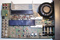
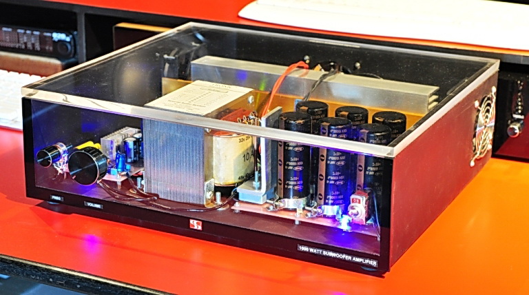
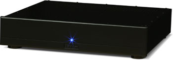
Audio stereo power amplifier

X . IIIIII

A Digital Amplifier Works

Most audiophiles and enthusiasts have grown up with at least a basic understanding of what an amplifier does. It takes a tiny alternating electrical signal that represents the moment-to-moment variations of musical frequencies and their amplitudes (volume levels), and increases their strength many times so they're powerful enough to drive the cones and domes of speakers back and forth to generate air pressure variations (waves), which replicate the original sound waves. Musical tones vary as slowly as 16 times per second (16 Hz)—a very low pipe-organ note—to as fast as 15,000 times per second (15 kHz) or more—the highest harmonics of a cymbal or a violin, for example.

Hi-Fi Analog Amplifiers

Until quite recently, the majority of high-fidelity audio amplifiers were analog, and most were of a type called Class A/B. What does that mean? Perhaps one of the easiest ways to understand how an analog audio amplifier works is to think of it as a kind of servo-controlled “valve” (the latter is what the Brits call vacuum tubes) that regulates stored up energy from the wall outlet and then releases it in measured amounts to your loudspeakers.

The amount being discharged is synchronized to the rapid variations of the incoming audio signal. This weak AC signal is used to modulate a circuit that releases power (voltage and amperage) stored up by the big capacitors and transformer in the amplifier’s power supply, power that is discharged in a way that exactly parallels the tiny modulations of the incoming audio signal.
This signal in the amplifier’s input stage applies a varying conductivity to the output circuit’s transistors, which release power from the amplifier’s power supply to move your loudspeaker’s cones and domes. It’s almost as though you were rapidly turning on a faucet (you turning the faucet is the audio signal), which releases all the stored up water pressure—the water tower or reservoir are the storage capacitors-- in a particular pattern, a kind of liquid code. For our purposes, that’s all we need to know about analog amplification.

Digital Amplification

Basically, a digital (Class D) amplifier takes an incoming analog signal and converts it into a digital representation comprised of pulse widths. Although there are a number of different design variations, Class D amplifiers are essentially switching amplifiers or Pulse Width Modulator (PWM) designs. The incoming analog audio signal is used to modulate a very high frequency Pulse-Width Modulated (PWM) carrier that works the output stage either fully on or off. Later on, this ultra-high-frequency carrier must be removed from the audio output with a reconstruction filter so that no ultra-high frequency switching components remain to corrupt the audio signals.

Differences in Pulse-Width and Pulse-Code Modulation

A digital amplifier’s operation is a little like the way a CD or digital recorder works with PCM (Pulse Code Modulation), the basis of all digital audio-recorded media. In PCM digital recording (a CD, for instance), the digital sampling ADC (analog-to-digital converter) “describes” the incoming analog voltage and frequency with a digital code of ones and zeroes. But in a digital amplifier, the Pulse-Width Modulator describes a low-frequency audio signal as the “widths of a pulse” so many milliseconds wide. (A high frequency would be a narrower pulse, fewer milliseconds wide -- see diagram). Once the analog audio signal (the curving red sine wave overriding the pulses) is “described” in terms of pulse widths, it is amplified and then converted back to analog form. During that process, a reconstruction filter must remove all the on-and-off pulses, leaving only the lower frequencies that represent the audio signal.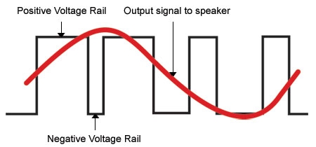

Voltage Rail Graph

As Axiom’s chief R&D engineer Tom Cumberland describes it, a digital amplifier is a “power DAC”, and of course a DAC (Digital-to-Analog Converter) is the basis of all digitally recorded media, whether we’re talking about CDs, hi-res audio, Blu-Ray soundtracks, DVD video, and so on. The view of some that “all digital amplifiers are crap” is not true. In fact, the clock rate of a good digital audio amplifier is typically in the range of 350 to 500 kHz (that’s 500,000 Hz). (Axiom’s ADA1500 digital amplifier uses a 450-kHz clock frequency.) By contrast, even the highest-resolution digital audio system (DVD-Audio and a variant used for Blu-ray soundtracks) runs at 192 kHz, which is far below the clock rate of a good digital amplifier.

Different Forms of Class D Amplification

Though we may think that “digital” means all the circuits in a digital amplifier work in on/off pulses, in fact there are a number of different types, including digital amplifiers that have analog elements.
A digital amplifier will have either analog or digital inputs. Good digital amplifiers with analog inputs can use analog feedback networks to lower the amplifier’s distortion, in much the same way that a Class A/B analog amplifier uses a negative feedback network to lessen the distortion. However, a digital amplifier that accepts only a digital input must rely on the incoming digital signal to lower distortion.

Feedback Networks

Why feedback networks? The reason they are used is that all parts in an amplifier have “tolerances,” which means that any particular part has a range or value in which it operates. Anyone who has examined such basic parts as resistors may have noticed they are specified as being “5%” or “10%” resistors, which means the specified resistor value is accurate within a range of 5% or 10%, respectively. Consequently, because of these variations in parts, a feedback network “looks at” the outgoing signal from the amplifiee -- the one that goes to your loudspeakers --and compares it to the incoming audio signal at the amplifier’s inputs. Any deviation in value away from the incoming signal is a distortion, so the negative feedback network applies inverse correction to compensate.
There are even differences in the operation of digital amplifiers. For example, the “ICE” digital amplifiers developed by the Ice Power division of Denmark’s Bang & Olufsen use a very complex negative feedback system due to parts tolerances. B&O holds patents on its “ICE” amplifier, which is basically a Class D switching design (Pulse Width Modulator) with variants that B&O claims reduces distortion to levels associated with Class A amps, while retaining the high efficiency of Class D switching designs.
“IR” (International Rectifier) is the system used by Axiom Audio in its ADA1500 digital amplifier. Axiom worked with International Rectifier to keep parts tolerances held to the very minimum amount, so that very little negative feedback would be used to correct for anomalies in the output. This approach also made the amplifier more robust in its operation without being subject to oscillations or instability.
Axiom and IR developed new silicon output devices that drive the MOSFETs in the output stage in such a way as to produce a perfect Pulse Width Modulated square wave at the output before the reconstruction filter.

Pros and Cons of ICE and IR Digital Amplifiers

One of the downsides to using a complex negative feedback network in a digital amplifier of the type used in ICE designs is a potential loss of efficiency. Performance may also suffer because of a slower clock rate.
In an IR type of digital design, which uses very little negative feedback or none at all, the clock rate is higher and efficiency increases. Moreover the high efficiency is combined with high power delivery and higher overall resolution. At full output, Axiom’s ADA1500 digital amp runs at about 95% efficiency (by comparison, class A/B analog amplifiers run between 50% and 60% efficiency; the remainder is wasted in heat).

Hasil gambar untuk foto hifi

X . IIIIIII

Class-D amplifier

as like as digital amplifier

A class-D amplifier or switching amplifier is an electronic amplifier in which the amplifying devices (transistors, usually MOSFETs) operate as electronic switches, and not as linear gain devices as in other amplifiers. The signal to be amplified is a train of constant amplitude pulses, so the active devices switch rapidly back and forth between a fully conductive and nonconductive state. The analog signal to be amplified is converted to a series of pulses by pulse width modulation, pulse density modulation or other method before being applied to the amplifier. After amplification, the output pulse train can be converted back to an analog signal by passing through a passive low pass filter consisting of inductors and capacitors.

Block diagram of a basic switching or PWM (class-D) amplifier Note: For Clarity, Signal Periods are not shown to scale

Basic operation

Class-D amplifiers work by generating a train of square pulses of fixed amplitude but varying width and separation, the low-frequency portion of whose frequency spectrum is essentially the signal to be amplified. The high-frequency portion serves no purpose other than to create a two level waveform. Because it has only two levels, it can be amplified by simple switching. The output of such a switch is an identical train of square pulses, except with greater amplitude. Such amplification results in a wave-form with the same frequency spectrum, but with every frequency uniformly magnified in amplitude.
A passive low-pass filter removes the unwanted high-frequency components, i.e., smooths the pulses out and recovers the desired low-frequency signal. To maintain high efficiency, the filter is made with purely reactive components (inductors and capacitors), which store the excess energy until it is needed instead of converting some of it into heat. The switching frequency is typically chosen to be ten or more times the highest frequency of interest in the input signal. This eases the requirements placed on the output filter. In cost sensitive applications the output filter is sometimes omitted. The circuit then relies on the inductance of the loudspeaker to keep the HF component from heating up the voice coil. It will also need to implement a form of three-level (class-BD) modulation which reduces HF output, particularly when no signal is present.
The structure of a class-D power stage is essentially identical to that of a synchronously rectified buck converter (a type of non-isolated switched-mode power supply (SMPS)). Whereas buck converters usually function as voltage regulators, delivering a constant DC voltage into a variable load and can only source current (one-quadrant operation), a class-D amplifier delivers a constantly changing voltage into a fixed load, where current and voltage can independently change sign (four-quadrant operation). A switching amplifier must not be confused with linear amplifiers that use an SMPS as their source of DC power. A switching amplifier may use any type of power supply (e.g., a car battery or an internal SMPS), but the defining characteristic is that the amplification process itself operates by switching.
Theoretical power efficiency of class-D amplifiers is 100%. That is to say, all of the power supplied to it is delivered to the load, none is turned to heat. This is because an ideal switch in its on state would conduct all the current but have no voltage loss across it, hence no heat would be dissipated. And when it is off, it would have the full supply voltage across it but no leak current flowing through it, and again no heat would be dissipated. Real-world power MOSFETs are not ideal switches, but practical efficiencies well over 90% are common. By contrast, linear AB-class amplifiers are always operated with both current flowing through and voltage standing across the power devices. An ideal class-B amplifier has a theoretical maximum efficiency of 78%. Class A amplifiers (purely linear, with the devices always "on") have a theoretical maximum efficiency of 50% and some versions have efficiencies below 20%.

Terminology

The term "class D" is sometimes misunderstood as meaning a "digital" amplifier. While some class-D amps may indeed be controlled by digital circuits or include digital signal processing devices, the power stage deals with voltage and current as a function of non-quantized time. The smallest amount of noise, timing uncertainty, voltage ripple or any other non-ideality immediately results in an irreversible change of the output signal. The same errors in a digital system will only lead to incorrect results when they become so large that a signal representing a digit is distorted beyond recognition. Up to that point, non-idealities have no impact on the transmitted signal. Generally, digital signals are quantized in both amplitude and wavelength, while analog signals are quantized in one (e.g. PWM) or (usually) neither quantity.

Signal modulation

The 2-level waveform is derived using pulse-width modulation (PWM), pulse density modulation (sometimes referred to as pulse frequency modulation), sliding mode control (more commonly called "self-oscillating modulation" in the trade.) or discrete-time forms of modulation such as delta-sigma modulation.
The most basic way of creating the PWM signal is to use a high speed comparator ("C" in the block-diagram above) that compares a high frequency triangular wave with the audio input. This generates a series of pulses of which the duty cycle is directly proportional with the instantaneous value of the audio signal. The comparator then drives a MOS gate driver which in turn drives a pair of high-power switches (usually MOSFETs). This produces an amplified replica of the comparator's PWM signal. The output filter removes the high-frequency switching components of the PWM signal and recovers the audio information that the speaker can use.
DSP-based amplifiers which generate a PWM signal directly from a digital audio signal (e. g. SPDIF) either use a counter to time the pulse length or implement a digital equivalent of a triangle-based modulator. In either case, the time resolution afforded by practical clock frequencies is only a few hundredths of a switching period, which is not enough to ensure low noise. In effect, the pulse length gets quantized, resulting in quantization distortion. In both cases, negative feedback is applied inside the digital domain, forming a noise shaper which has lower noise in the audible frequency range.

Design challenges

Switching speed

Two significant design challenges for MOSFET driver circuits in class-D amplifiers are keeping dead times and linear mode operation as short as possible. "Dead time" is the period during a switching transition when both output MOSFETs are driven into Cut-Off Mode and both are "off". Dead times need to be as short as possible to maintain an accurate low-distortion output signal, but dead times that are too short cause the MOSFET that is switching on to start conducting before the MOSFET that is switching off has stopped conducting. The MOSFETs effectively short the output power supply through themselves in a condition known as "shoot-through". Meanwhile, the MOSFET drivers also need to drive the MOSFETs between switching states as fast as possible to minimize the amount of time a MOSFET is in Linear Mode—the state between Cut-Off Mode and Saturation Mode where the MOSFET is neither fully on nor fully off and conducts current with a significant resistance, creating significant heat. Driver failures that allow shoot-through and/or too much linear mode operation result in excessive losses and sometimes catastrophic failure of the MOSFETs.

Electromagnetic interference

The switching power stage generates both high dV/dt and dI/dt, which give rise to radiated emission whenever any part of the circuit is large enough to act as an antenna. In practice, this means the connecting wires and cables will be the most efficient radiators so most effort should go into preventing high-frequency signals reaching those:

Avoid capacitive coupling from switching signals into the wiring.
Avoid inductive coupling from various current loops in the power stage into the wiring.
Use one unbroken ground plane and group all connectors together, in order to have a common RF reference for decoupling capacitors
Include the equivalent series inductance of filter capacitors and the parasitic capacitance of filter inductors in the circuit model before selecting components.
Wherever ringing is encountered, locate the inductive and capacitive parts of the resonant circuit that causes it, and use parallel RC or series RL snubbers to reduce the Q of the resonance.
Do not make the MOSFETs switch any faster than needed to fulfil efficiency or distortion requirements. Distortion is more easily reduced using negative feedback than by speeding up switching.

Power supply design

Class-D amplifiers place an additional requirement on their power supply, namely that it be able to sink energy returning from the load. Reactive (capacitive or inductive) loads store energy during part of a cycle and release some of this energy back later. Linear amplifiers will dissipate this energy away, class-D amplifiers return it to the power supply which should somehow be able to store it. In addition, half-bridge class D amps transfer energy from one supply rail (e.g. the positive rail) to the other (e.g. the negative) depending on the sign of the output current. This happens regardless of whether the load is resistive or not. The supply should either have enough capacitive storage on both rails, or be able to transfer this energy back.

Error control

The actual output of the amplifier is not just dependent on the content of the modulated PWM signal. The power supply voltage directly amplitude-modulates the output voltage, dead time errors make the output impedance non-linear and the output filter has a strongly load-dependent frequency response. An effective way to combat errors, regardless of their source, is negative feedback. A feedback loop including the output stage can be made using a simple integrator. To include the output filter, a PID controller is used, sometimes with additional integrating terms. The need to feed the actual output signal back into the modulator makes the direct generation of PWM from a SPDIF source unattractive. Mitigating the same issues in an amplifier without feedback requires addressing each separately at the source. Power supply modulation can be partially canceled by measuring the supply voltage to adjust signal gain before calculating the PWM and distortion can be reduced by switching faster. The output impedance cannot be controlled other than through feedback.

Advantages

The major advantage of a class-D amplifier is that it can be more efficient than an analog amplifier, with less power dissipated as heat in the active devices. Given that large heat sinks are not required, Class-D amplifiers are much lighter weight than analog amplifiers, an important consideration with portable sound reinforcement system equipment and bass amplifiers. Output stages such as those used in pulse generators are examples of class-D amplifiers. However, the term mostly applies to power amplifiers intended to reproduce audio signals with a bandwidth well below the switching frequency.
Despite the complexity involved, a properly designed class-D amplifier offers the following benefits:

Reduced power waste as heat dissipation and hence:
Reduction in cost, size and weight of the amplifier due to smaller (or no) heat sinks, and compact circuitry,
Very high power conversion efficiency, usually better than 90% above one quarter of the amplifier's maximum power, and around 50% at low power levels.
Can operate from a digital signal source without requiring a digital-to-analog converter (DAC) to convert the signal to analog form first.

Boss Audio mono amp. The output stage is top left, the output chokes are the two yellow toroids underneath.

Uses

Home theatre in a box systems. These economical home cinema systems are almost universally equipped with class-D amplifiers. On account of modest performance requirements and straightforward design, direct conversion from digital audio to PWM without feedback is most common.
Mobile phones. The internal loudspeaker is driven by up to 1 W. Class D is used to preserve battery lifetime.
Hearing aids. The miniature loudspeaker (known as the receiver) is directly driven by a class-D amplifier to maximise battery life and can provide saturation levels of 130 dB SPL or more.
Powered speakers
High-end audio is generally conservative with regards to adopting new technologies but class-D amplifiers have made an appearance
Active subwoofers
Sound Reinforcement and Live Sound. For very high power amplification the powerloss of AB amplifiers are unacceptable. Amps with several kilowatts of output power are available as class-D. The Crest Audio CD3000, for example, is a class-D power amplifier that is rated at 1500 W per channel, yet it weighs only 21 kg (46 lb). Similarly, the Powersoft K10 is a class-D power amplifier that is rated at 6000 W per 2-Ohm channel, yet it weighs only 12 kg (26.5 lb).
Bass amplifiers. Again, an area where portability is important. Example: Yamaha BBT500H bass amplifier which is rated at 500 W, and yet it weighs less than 5 kg (11 lb). The Promethean P500H by Ibanez is also capable of delivering 500 W into a 4 Ohm load, and weighs only 2.9 kg (6.4 lb). Gallien Krueger MB500 and Eden WTX500, also rated at 500 W weighs no more than 2 kg (4.4 lb).

Class-T amplifier

Two Tripath chipset Class T stereo amplifier modules. TA2024 6+6W to the left, TA2020 20+20W to the right

Class T was a registered trademark for a switching (class-D) audio amplifier, used for Tripath's amplifier technologies (patent filed on Jun 20, 1996). Similar designs have now been widely adopted by different manufacturers.
The covered products use a class-D amplifiers combined with proprietary techniques to control the pulse width modulation to produce what is claimed to be better performance than other class-D amplifier designs. Among the publicly disclosed differences is real time control of the switching frequency depending on the input signal and amplified output. One of the amplifiers, the TA2020, was named one of the twenty-five chips that 'shook the world" by the IEEE Spectrum magazine.
The control signals in Class T amplifiers may be computed using digital signal processing or fully analog techniques. Currently available implementations use a loop similar to a higher order Delta-Sigma (ΔΣ) (or sigma-delta) modulator, with an internal digital clock to control the sample comparator. The two key aspects of this topology are that (1), feedback is taken directly from the switching node rather than the filtered output, and (2), the higher order loop provides much higher loop gain at high audio frequencies than would be possible in a conventional single pole amplifier.

Blaupunkt PA2150 T-Amp, "Powered by Tripath"

Tripath's stock and intellectual property were purchased later that year by Cirrus Logic.

X . IIIIIIII

Delta-sigma modulation

Delta-sigma (ΔΣ; or sigma-delta, ΣΔ) modulation is a method for encoding analog signals into digital signals as found in an analog-to-digital converter (ADC). It is also used to transfer high bit-count low frequency digital signals into lower bit-count higher frequency digital signals as part of the process to convert digital signals into analog as part of a digital-to-analog converter (DAC).
In a conventional ADC, an analog signal is integrated, or sampled, with a sampling frequency and subsequently quantized in a multi-level quantizer into a digital signal. This process introduces quantization error noise. The first step in a delta-sigma modulation is delta modulation. In delta modulation the change in the signal (its delta) is encoded, rather than the absolute value. The result is a stream of pulses, as opposed to a stream of numbers as is the case with PCM. In delta-sigma modulation, the accuracy of the modulation is improved by passing the digital output through a 1-bit DAC and adding (sigma) the resulting analog signal to the input signal, thereby reducing the error introduced by the delta-modulation.
Primarily because of its cost efficiency and reduced circuit complexity, this technique has found increasing use in modern electronic components such as DACs, ADCs, frequency synthesizers, switched-mode power supplies and motor controllers.
Both ADCs and DACs can employ delta-sigma modulation. A delta-sigma ADC first encodes an analog signal using high-frequency delta-sigma modulation, and then applies a digital filter to form a higher-resolution but lower sample-frequency digital output. On the other hand, a delta-sigma DAC encodes a high-resolution digital input signal into a lower-resolution but higher sample-frequency signal that is mapped to voltages, and then smoothed with an analog filter. In both cases, the temporary use of a lower-resolution signal simplifies circuit design and improves efficiency.
The coarsely-quantized output of a delta-sigma modulator is occasionally used directly in signal processing or as a representation for signal storage. For example, the Super Audio CD (SACD) stores the output of a delta-sigma modulator directly on a disk.

Motivation

Why convert an analog signal into a stream of pulses?

In brief, because it is very easy to regenerate pulses at the receiver into the ideal form transmitted. The only part of the transmitted waveform required at the receiver is the time at which the pulse occurred. Given the timing information the transmitted waveform can be reconstructed electronically with great precision. In contrast, without conversion to a pulse stream but simply transmitting the analog signal directly, all noise in the system is added to the analog signal, permanently reducing its quality.
Each pulse is made up of a step up followed after a short interval by a step down. It is possible, even in the presence of electronic noise, to recover the timing of these steps and from that regenerate the transmitted pulse stream almost noiselessly. Then the accuracy of the transmission process reduces to the accuracy with which the transmitted pulse stream represents the input waveform.

Why delta-sigma modulation?

Delta-sigma modulation converts the analog voltage into a pulse frequency and is alternatively known as Pulse Density modulation or Pulse Frequency modulation. In general, frequency may vary smoothly in infinitesimal steps, as may voltage, and both may serve as an analog of an infinitesimally varying physical variable such as acoustic pressure, light intensity, etc. The substitution of frequency for voltage is thus entirely natural and carries in its train the transmission advantages of a pulse stream. The different names for the modulation method are the result of pulse frequency modulation by different electronic implementations, which all produce similar transmitted waveforms.

Why the delta-sigma analog to digital conversion?

The ADC converts the mean of an analog voltage into the mean of an analog pulse frequency and counts the pulses in a known interval so that the pulse count divided by the interval gives an accurate digital representation of the mean analog voltage during the interval. This interval can be chosen to give any desired resolution or accuracy. The method is cheaply produced by modern methods; and it is widely used.

Analog to digital conversion

Description

The ADC generates a pulse stream in which the frequency,

f

, of pulses in the stream is proportional to the analog voltage input,

v

, so that

f=k\cdot v

, where k is a constant for the particular implementation.
A counter sums the number of pulses that occur in a predetermined period,

P

so that the sum,

\Sigma

, is

P\cdot f=k\cdot P\cdot v

k\cdot P

is chosen so that a digital display of the count,

\Sigma

, is a display of

v

with a predetermined scaling factor. Because

P

may take any designed value it may be made large enough to give any desired resolution or accuracy.
Each pulse of the pulse stream has a known, constant amplitude

V

and duration

\operatorname {d} t

, and thus has a known integral

V\operatorname {d} t

but variable separating interval.
In a formal analysis an impulse such as integral

V\operatorname {d} t

is treated as the Dirac δ (delta) function and is specified by the step produced on integration. Here we indicate that step as

\Delta =\int V\operatorname {d} t

.
The interval between pulses, p, is determined by a feedback loop arranged so that

p={\frac {1}{f}}={\frac {1}{k\cdot v}}

.
The action of the feedback loop is to monitor the integral of v and when that integral has incremented by

\Delta

, which is indicated by the integral waveform crossing a threshold, then subtracting

\Delta

from the integral of v so that the combined waveform sawtooths between the threshold and ( threshold -

\Delta

). At each step a pulse is added to the pulse stream.
Between impulses, the slope of the integral is proportional to

v

, that is, for some

A

it equals

A\cdot v={\frac {\Delta }{p}}=\Delta \cdot f=\Delta \cdot k\cdot v

. Whence

A=\Delta \cdot k

.
It is the pulse stream which is transmitted for delta-sigma modulation but the pulses are counted to form sigma in the case of analogue to digital conversion.

Analysis

Fig. 1: Block diagram and waveforms for a sigma delta ADC.

Fig. 1a: Effect of clocking impulses

Shown below the block diagram illustrated in Fig. 1 are waveforms at points designated by numbers 1 to 5 for an input of 0.2 volts on the left and 0.4 volts on the right.
In most practical applications the summing interval is large compared with the impulse duration and for signals which are a significant fraction of full scale the variable separating interval is also small compared with the summing interval. The Nyquist–Shannon sampling theorem requires two samples to render a varying input signal. The samples appropriate to this criterion are two successive Σ counts taken in two successive summing intervals. The summing interval, which must accommodate a large count in order to achieve adequate precision, is inevitably long so that the converter can only render relatively low frequencies. Hence it is convenient and fair to represent the input voltage (1) as constant over a few impulses.
Consider first the closed feedback loop consisting of the analogue adder/subtracter, the integrator, the threshold crossing detector and the impulse generator.
On the left 1 is the input and for this short interval is constant at 0.2 V. The stream of delta impulses generated at each threshold crossing is shown at 2 and the difference between 1 and 2 is shown at 3. This difference is integrated to produce the waveform 4. The threshold detector generates a pulse 5 which starts as the waveform 4 crosses the threshold and is sustained until the waveform 4 falls below the threshold. Within the loop 5 triggers the impulse generator to produce a fixed strength impulse.
On the right the input is now 0.4 V and the sum during the impulse is −0.6 V as opposed to −0.8 V on the left. Thus the negative slope during the impulse is lower on the right than on the left.
Also the sum is 0.4 V on the right during the interval as opposed to 0.2 V on the left. Thus the positive slope outside the impulse is higher on the right than on the left.
The resultant effect is that the integral (4) crosses the threshold more quickly on the right than on the left. A full analysis would show that in fact the interval between threshold crossings on the right is half that on the left. Thus the frequency of impulses is doubled. Hence the count increments at twice the speed on the right to that on the left which is consistent with the input voltage being doubled.The overall effect of the negative feedback loop is to maintain the running integral of the impulse train equal to within one impulse to the running integral of the input analogue signal. Also the frequency of the impulse train is proportional to the bandwidth limited amplitude of the input signal.Bandwidth limitation occurs because the Nyquist–Shannon sampling theorem requires 2 impulses per period to define the highest frequency passed.
Construction of the waveforms illustrated at (4) is aided by concepts associated with the Dirac delta function in that all impulses of the same strength produce the same step when integrated, by definition. Then (4) is constructed using an intermediate step (6) in which each integrated impulse is represented by a step of the assigned strength which decays to zero at the rate determined by the input voltage. The effect of the finite duration of the impulse is constructed in (4) by drawing a line from the base of the impulse step at zero volts to intersect the decay line from (6) at the full duration of the impulse.
Now consider the circuit outside the loop. The summing interval is a prefixed time and at its expiry the count is strobed into the buffer and the counter reset. It is necessary that the ratio between the impulse interval and the summing interval is equal to the maximum (full scale) count. It is then possible for the impulse duration and the summing interval to be defined by the same clock with a suitable arrangement of logic and counters. This has the advantage that neither interval has to be defined with absolute precision as only the ratio is important. Then to achieve overall accuracy it is only necessary that the amplitude of the impulse be accurately defined. As stated, Fig. 1 is a simplified block diagram of the delta-sigma ADC in which the various functional elements have been separated out for individual treatment and which tries to be independent of any particular implementation. Many particular implementations seek to define the impulse duration and the summing interval from the same clock as discussed above but in such a way that the start of the impulse is delayed until the next occurrence of the appropriate clock pulse boundary. The effect of this delay is illustrated in Fig. 1a for a sequence of impulses which occur at a nominal 2.5 clock intervals, firstly for impulses generated immediately the threshold is crossed as previously discussed and secondly for impulses delayed by the clock. The effect of the delay is firstly that the ramp continues until the onset of the impulse, secondly that the impulse produces a fixed amplitude step so that the integral retains the excess it acquired during the impulse delay and so the ramp restarts from a higher point and is now on the same locus as the free running integral. The effect is that, for this example, the undelayed impulses will occur at clock points 0, 2.5, 5, 7.5, 10, etc. and the clocked impulses will occur at 0, 3, 5, 8, 10, etc. The maximum error that can occur due to clocking is marginally less than one count. Although the Sigma-Delta converter is generally implemented using a common clock to define the impulse duration and the summing interval it is not absolutely necessary and an implementation in which the durations are independently defined avoids one source of noise, the noise generated by waiting for the next common clock boundary. Where noise is a primary consideration that overrides the need for absolute amplitude accuracy; e.g., in bandwidth limited signal transmission, separately defined intervals may be implemented.

Practical Implementation

Fig. 1b: circuit diagram

Fig. 1c: ADC waveforms

A circuit diagram for a practical implementation is illustrated, Fig 1b and the associated waveforms Fig. 1c. This circuit diagram is mainly for illustration purposes, details of particular manufacturers implementations will usually be available from the particular manufacturer. A scrap view of an alternative front end is shown in Fig. 1b which has the advantage that the voltage at the switch terminals are relatively constant and close to 0.0 V. Also the current generated through R by −V_ref is constant at −V_ref/R so that much less noise is radiated to adjacent parts of the circuit. Then this would be the preferred front end in practice but, in order to show the impulse as a voltage pulse so as to be consistent with previous discussion, the front end given here, which is an electrical equivalent, is used.
The waveforms shown in Fig 1c are unusually complex because they are intended to illustrate the loop behaviour under extreme conditions,V_in saturated on at full scale, 1.0V, and saturated off at zero. The intermediate state is also indicated,V_in at 0.4V, and is the usual operating condition between 0 and 1.0v where it is very similar to the operation of the illustrative block diagram, Fig 1.
From the top of Fig 1c the waveforms, labelled as they are on the circuit diagram, are:-
The clock.
(a) V_in. This is shown as varying from 0.4 V initially to 1.0 V and then to zero volts to show the effect on the feedback loop.
(b) The impulse waveform. It will be discovered how this acquires its form as we traverse the feedback loop.
(c) The current into the capacitor, I_c, is the linear sum of the impulse voltage upon R and V_in upon R. To show this sum as a voltage the product R × I_c is plotted. The input impedance of the amplifier is regarded as so high that the current drawn by the input is neglected.The capacitor is connected between the negative input terminal of the amplifier and its output terminal. With this connection it provides a negative feedback path around the amplifier. The input voltage change is equal to the output voltage change divided by the amplifier gain. With very high amplifier gain the change in input voltage can be neglected and so the input voltage is held close to the voltage on the positive input terminal which in this case is held at 0V. Because the voltage at the input terminal is 0V the voltage across R is simply V_in so that the current into the capacitor is the input voltage divided by the resistance of R.
(d) The negated integral of I_c. This negation is standard for the op. amp. implementation of an integrator and comes about because the current into the capacitor at the amplifier input is the current out of the capacitor at the amplifier output and the voltage is the integral of the current divided by the capacitance of C.
(e) The comparator output. The comparator is a very high gain amplifier with its plus input terminal connected for reference to 0.0 V. Whenever the negative input terminal is taken negative with respect the positive terminal of the amplifier the output saturates positive and conversely negative saturation for positive input. Thus the output saturates positive whenever the integral (d) goes below the 0 V reference level and remains there until (d) goes positive with respect to the reference level.
(f) The impulse timer is a D type positive edge triggered flip flop. Input information applied at D is transferred to Q on the occurrence of the positive edge of the clock pulse. thus when the comparator output (e) is positive Q goes positive or remains positive at the next positive clock edge. Similarly, when (e) is negative Q goes negative at the next positive clock edge. Q controls the electronic switch to generate the current impulse into the integrator. Examination of the waveform (e) during the initial period illustrated, when V_in is 0.4 V, shows (e) crossing the threshold well before the trigger edge (positive edge of the clock pulse) so that there is an appreciable delay before the impulse starts. After the start of the impulse there is further delay while (e) climbs back past the threshold. During this time the comparator output remains high but goes low before the next trigger edge. At that next trigger edge the impulse timer goes low to follow the comparator. Thus the clock determines the duration of the impulse. For the next impulse the threshold is crossed immediately before the trigger edge and so the comparator is only briefly positive. V_in (a) goes to full scale, +V_ref, shortly before the end of the next impulse. For the remainder of that impulse the capacitor current (c) goes to zero and hence the integrator slope briefly goes to zero. Following this impulse the full scale positive current is flowing (c) and the integrator sinks at its maximum rate and so crosses the threshold well before the next trigger edge. At that edge the impulse starts and the Vin current is now matched by the reference current so that the net capacitor current (c) is zero. Then the integration now has zero slope and remains at the negative value it had at the start of the impulse. This has the effect that the impulse current remains switched on because Q is stuck positive because the comparator is stuck positive at every trigger edge. This is consistent with contiguous, butting impulses which is required at full scale input.
Eventually Vin (a) goes to zero which means that the current sum (c) goes fully negative and the integral ramps up. It shortly thereafter crosses the threshold and this in turn is followed by Q, thus switching the impulse current off. The capacitor current (c) is now zero and so the integral slope is zero, remaining constant at the value it had acquired at the end of the impulse.
(g) The countstream is generated by gating the negated clock with Q to produce this waveform. Thereafter the summing interval, sigma count and buffered count are produced using appropriate counters and registers. The V_in waveform is approximated by passing the countstream (g) into a low pass filter, however it suffers from the defect discussed in the context of Fig. 1a. One possibility for reducing this error is to halve the feedback pulse length to half a clock period and double its amplitude by halving the impulse defining resistor thus producing an impulse of the same strength but one which never butts onto its adjacent impulses. Then there will be a threshold crossing for every impulse. In this arrangement a monostable flip flop triggered by the comparator at the threshold crossing will closely follow the threshold crossings and thus eliminate one source of error, both in the ADC and the sigma delta modulator.

Remarks

In this section we have mainly dealt with the analogue to digital converter as a stand-alone function which achieves astonishing accuracy with what is now a very simple and cheap architecture. Initially the Delta-Sigma configuration was devised by INOSE et al. to solve problems in the accurate transmission of analog signals. In that application it was the pulse stream that was transmitted and the original analog signal recovered with a low pass filter after the received pulses had been reformed. This low pass filter performed the summation function associated with Σ. The highly mathematical treatment of transmission errors was introduced by them and is appropriate when applied to the pulse stream but these errors are lost in the accumulation process associated with Σ to be replaced with the errors associated with the mean of means when discussing the ADC. For those uncomfortable with this assertion consider this.
It is well known that by Fourier analysis techniques the incoming waveform can be represented over the summing interval by the sum of a constant plus a fundamental and harmonics each of which has an exact integer number of cycles over the sampling period. It is also well known that the integral of a sine wave or cosine wave over one or more full cycles is zero. Then the integral of the incoming waveform over the summing interval reduces to the integral of the constant and when that integral is divided by the summing interval it becomes the mean over that interval. The interval between pulses is proportional to the inverse of the mean of the input voltage during that interval and thus over that interval, ts, is a sample of the mean of the input voltage proportional to V/ts. Thus the average of the input voltage over the summing period is VΣ/N and is the mean of means and so subject to little variance.
Unfortunately the analysis for the transmitted pulse stream has, in many cases, been carried over, uncritically, to the ADC.
It was indicated in section 2.2 Analysis that the effect of constraining a pulse to only occur on clock boundaries is to introduce noise, that generated by waiting for the next clock boundary. This will have its most deleterious effect on the high frequency components of a complex signal. Whilst the case has been made for clocking in the ADC environment, where it removes one source of error, namely the ratio between the impulse duration and the summing interval, it is deeply unclear what useful purpose clocking serves in a single channel transmission environment since it is a source of both noise and complexity but it is conceivable that it would be useful in a TDM (time division multiplex) environment.
A very accurate transmission system with constant sampling rate may be formed using the full arrangement shown here by transmitting the samples from the buffer protected with redundancy error correction. In this case there will be a trade off between bandwidth and N, the size of the buffer. The signal recovery system will require redundancy error checking, digital to analog conversion, and sample and hold circuitry. A possible further enhancement is to include some form of slope regeneration. This amounts to PCM (pulse code modulation) with digitization performed by a sigma-delta ADC.
The above description shows why the impulse is called delta. The integral of an impulse is a step. A one bit DAC may be expected to produce a step and so must be a conflation of an impulse and an integration. The analysis which treats the impulse as the output of a 1-bit DAC hides the structure behind the name (sigma delta) and cause confusion and difficulty interpreting the name as an indication of function. This analysis is very widespread but is deprecated.
A modern alternative method for generating voltage to frequency conversion is discussed in synchronous voltage to frequency converter (SVFC) which may be followed by a counter to produce a digital representation in a similar manner to that described above.

Digital to analog conversion

Discussion

Delta-sigma modulators are often used in digital to analog converters (DACs). In general, a DAC converts a digital number representing some analog value into that analog value. For example, the analog voltage level into a speaker may be represented as a 20 bit digital number, and the DAC converts that number into the desired voltage. To actually drive a load (like a speaker) a DAC is usually connected to or integrated with an electronic amplifier.
This can be done using a delta-sigma modulator in a Class D Amplifier. In this case, a multi-bit digital number is input to the delta-sigma modulator, which converts it into a faster sequence of 0s and 1s. These 0s and 1s are then converted into analog voltages. The conversion, usually with MOSFET drivers, is very efficient in terms of power because the drivers are usually either fully on or fully off, and in these states have low power loss.
The resulting two-level signal is now like the desired signal, but with higher frequency components to change the signal so that it only has two levels. These added frequency components arise from the quantization error of the delta-sigma modulator, but can be filtered away by a simple low-pass filter. The result is a reproduction of the original, desired analog signal from the digital values.
The circuit itself is relatively inexpensive. The digital circuit is small, and the MOSFETs used for the power amplification are simple. This is in contrast to a multi-bit DAC which can have very stringent design conditions to precisely represent digital values with a large number of bits.
The use of a delta-sigma modulator in the digital to analog conversion has enabled a cost-effective, low power, and high performance solution.

Relationship to Δ-modulation

Fig. 2: Derivation of ΔΣ- from Δ-modulation

ΔΣ modulation (SDM) is inspired by Δ modulation (DM), as shown in Fig. 2. If quantization were homogeneous (e.g., if it were linear), the following would be a sufficient derivation of the equivalence of DM and SDM:

Start with a block diagram of a Δ-modulator/demodulator.
The linearity property of integration ( $\scriptstyle \int a\,+\,\int b\,=\,\int (a\,+\,b)$ ) makes it possible to move the integrator, which reconstructs the analog signal in the demodulator section, in front of the Δ-modulator.
Again, the linearity property of the integration allows the two integrators to be combined and a ΔΣ-modulator/demodulator block diagram is obtained.

However, the quantizer is not homogeneous, and so this explanation is flawed. It's true that ΔΣ is inspired by Δ-modulation, but the two are distinct in operation. From the first block diagram in Fig. 2, the integrator in the feedback path can be removed if the feedback is taken directly from the input of the low-pass filter. Hence, for delta modulation of input signal

\scriptstyle u

, the low-pass filter sees the signal

y_{\text{DM}}=\int \operatorname {Quantize} \left(u-y_{\text{DM}}\right).\,

However, sigma-delta modulation of the same input signal places at the low-pass filter

y_{\text{SDM}}=\operatorname {Quantize} \left(\int \left(u-y_{\text{SDM}}\right)\right).\,

In other words, SDM and DM swap the position of the integrator and quantizer. The net effect is a simpler implementation that has the added benefit of shaping the quantization noise away from signals of interest (i.e., signals of interest are low-pass filtered while quantization noise is high-pass filtered). This effect becomes more dramatic with increased oversampling, which allows for quantization noise to be somewhat programmable. On the other hand, Δ-modulation shapes both noise and signal equally.
Additionally, the quantizer (e.g., comparator) used in DM has a small output representing a small step up and down the quantized approximation of the input while the quantizer used in SDM must take values outside of the range of the input signal, as shown in Fig. 3.

Fig. 3: An example of SDM of 100 samples of one period a sine wave. 1-bit

samples (e.g., comparator output) overlaid with sine wave where logic high (e.g.,

\scriptstyle +V_{CC}

) represented by blue and logic low (e.g.,

\scriptstyle -V_{CC}

) represented by white.

In general, ΔΣ has some advantages versus Δ modulation:

The whole structure is simpler:
- Only one integrator is needed
- The demodulator can be a simple linear filter (e.g., RC or LC filter) to reconstruct the signal
- The quantizer (e.g., comparator) can have full-scale outputs
The quantized value is the integral of the difference signal, which makes it less sensitive to the rate of change of the signal.

Principle

The principle of the ΔΣ architecture is explained at length in section 2. Initially, when a sequence starts, the circuit will have an arbitrary state which is dependent on the integral of all previous history. In mathematical terms this corresponds to the arbitrary integration constant of the indefinite integral. This follows from the fact that at the heart of the method there is an integrator which can have any arbitrary state dependent on previous input, see Fig. 1c (d). From the occurrence of the first pulse onward the frequency of the pulse stream is proportional to the input voltage to be transformed. A demonstration applet is available online to simulate the whole architecture.

Variations

There are many kinds of ADC that use this delta-sigma structure. The above analysis focuses on the simplest 1st-order, 2-level, uniform-decimation sigma-delta ADC. Many ADCs use a second-order 5-level sinc3 sigma-delta structure.

2nd order and higher order modulator

Fig. 4: Block diagram of a 2nd order ΔΣ modulator

The number of integrators, and consequently, the numbers of feedback loops, indicates the order of a ΔΣ-modulator; a 2nd order ΔΣ modulator is shown in Fig. 4. First order modulators are unconditionally stable, but stability analysis must be performed for higher order modulators.

3-level and higher quantizer

The modulator can also be classified by the number of bits it has in output, which strictly depends on the output of the quantizer. The quantizer can be realized with a N-level comparator, thus the modulator has log₂N-bit output. A simple comparator has 2 levels and so is 1 bit quantizer; a 3-level quantizer is called a "1.5" bit quantizer; a 4-level quantizer is a 2 bit quantizer; a 5-level quantizer is called a "2.5 bit" quantizer.

Decimation structures

The conceptually simplest decimation structure is a counter that is reset to zero at the beginning of each integration period, then read out at the end of the integration period.
The multi-stage noise shaping (MASH) structure has a noise shaping property, and is commonly used in digital audio and fractional-N frequency synthesizers. It comprises two or more cascaded overflowing accumulators, each of which is equivalent to a first-order sigma delta modulator. The carry outputs are combined through summations and delays to produce a binary output, the width of which depends on the number of stages (order) of the MASH. Besides its noise shaping function, it has two more attractive properties:

simple to implement in hardware; only common digital blocks such as accumulators, adders, and D flip-flops are required
unconditionally stable (there are no feedback loops outside the accumulators)

A very popular decimation structure is the sinc filter. For 2nd order modulators, the sinc3 filter is close to optimum.

Quantization theory formulas

Main article: Quantization (signal processing)

When a signal is quantized, the resulting signal approximately has the second-order statistics of a signal with independent additive white noise. Assuming that the signal value is in the range of one step of the quantized value with an equal distribution, the root mean square value of this quantization noise is

{\displaystyle e_{\mathrm {rms} }\,={\sqrt {\,{\frac {1}{\Delta }}\int _{-\Delta /2}^{+\Delta /2}e^{2}\,de\,}}=\,{\frac {\Delta }{2{\sqrt {3}}}}}

In reality, the quantization noise is of course not independent of the signal; this dependence is the source of idle tones and pattern noise in Sigma-Delta converters.
The over-sampling ratio (OSR), where

f_{\mathrm {s} }

is the sampling frequency and

2f_{0}

is Nyquist rate, is defined by

\mathrm {OSR} \,=\,{\frac {f_{s}}{2f_{0}}}\,=\,{\frac {1}{2f_{0}\tau }}

The RMS noise voltage within the band of interest can be expressed in terms of OSR

\mathrm {n_{0}} \,=\,{\frac {e_{rms}}{\sqrt {OSR}}}

Oversampling

Fig. 5: Noise shaping curves and noise spectrum in ΔΣ modulator

Oversampling

Let's consider a signal at frequency

\scriptstyle f_{0}

and a sampling frequency of

\scriptstyle f_{\mathrm {s} }

much higher than Nyquist rate (see fig. 5). ΔΣ modulation is based on the technique of oversampling to reduce the noise in the band of interest (green), which also avoids the use of high-precision analog circuits for the anti-aliasing filter. The quantization noise is the same both in a Nyquist converter (in yellow) and in an oversampling converter (in blue), but it is distributed over a larger spectrum. In ΔΣ-converters, noise is further reduced at low frequencies, which is the band where the signal of interest is, and it is increased at the higher frequencies, where it can be filtered. This technique is known as noise shaping.
For a first order delta sigma modulator, the noise is shaped by a filter with transfer function

\scriptstyle H_{n}(z)\,=\,\left[1-z^{-1}\right]

. Assuming that the sampling frequency

\scriptstyle f_{s}\,\gg \,f_{0}

, the quantization noise in the desired signal bandwidth can be approximated as:

\mathrm {n_{0}} \,=\,e_{rms}{\frac {\pi }{\sqrt {3}}}\,(2f_{0}\tau )^{\frac {3}{2}}

.
Similarly for a second order delta sigma modulator, the noise is shaped by a filter with transfer function

\scriptstyle H_{n}(z)\,=\,\left[1-z^{-1}\right]^{2}

. The in-band quantization noise can be approximated as:

\mathrm {n_{0}} \,=\,e_{rms}{\frac {\pi ^{2}}{\sqrt {5}}}\,(2f_{0}\tau )^{\frac {5}{2}}

.
In general, for a

\scriptstyle \mathrm {N}

-order ΔΣ-modulator, the variance of the in-band quantization noise:

\mathrm {n_{0}} \,=\,e_{rms}{\frac {\pi ^{N}}{\sqrt {2N+1}}}\,(2f_{0}\tau )^{\frac {2N+1}{2}}

.
When the sampling frequency is doubled, the signal to quantization noise is improved by

\scriptstyle 10\log(2^{2N+1})\,dB

for a

\scriptstyle \mathrm {N}

-order ΔΣ-modulator. The higher the oversampling ratio, the higher the signal-to-noise ratio and the higher the resolution in bits.
Another key aspect given by oversampling is the speed/resolution tradeoff. In fact, the decimation filter put after the modulator not only filters the whole sampled signal in the band of interest (cutting the noise at higher frequencies), but also reduces the frequency of the signal increasing its resolution. This is obtained by a sort of averaging of the higher data rate bitstream.

Example of decimation

Let's have, for instance, an 8:1 decimation filter and a 1-bit bitstream; if we have an input stream like 10010110, counting the number of ones, we get 4. Then the decimation result is 4/8 = 0.5. We can then represent it with a 3-bits number 100 (binary), which means half of the largest possible number. In other words,

the sample frequency is reduced by a factor of eight
the serial (1-bit) input bus becomes a parallel (3-bits) output bus.

Naming

The technique was first presented in the early 1960s by professor Haruhiko Yasuda while he was a student at Waseda University, Tokyo, Japan. The name Delta-Sigma comes directly from the presence of a Delta modulator and an integrator, as firstly introduced by Inose et al. in their patent application. That is, the name comes from integrating or "summing" differences, which are operations usually associated with Greek letters Sigma and Delta respectively. Both names Sigma-Delta and Delta-Sigma are frequently used.

Pulse-density modulation

Pulse-density modulation, or PDM, is a form of modulation used to represent an analog signal with a binary signal. In a PDM signal, specific amplitude values are not encoded into codewords of pulses of different weight as they would be in pulse-code modulation (PCM); rather, the relative density of the pulses corresponds to the analog signal's amplitude. The output of a 1-bit DAC is the same as the PDM encoding of the signal. Pulse-width modulation (PWM) is a special case of PDM where the switching frequency is fixed and all the pulses corresponding to one sample are contiguous in the digital signal. For a 50% voltage with a resolution of 8-bits, a PWM waveform will turn on for 128 clock cycles and then off for the remaining 128 cycles. With PDM and the same clock rate the signal would alternate between on and off every other cycle. The average is 50% for both waveforms, but the PDM signal switches more often. For 100% or 0% level, they are the same.

Description

In a pulse-density modulation bitstream a 1 corresponds to a pulse of positive polarity (+A) and a 0 corresponds to a pulse of negative polarity (-A). Mathematically, this can be represented as:

x[n]=-A(-1)^{a[n]}\

where x[n] is the bipolar bitstream (either -A or +A) and a[n] is the corresponding binary bitstream (either 0 or 1).

A run consisting of all 1s would correspond to the maximum (positive) amplitude value, all 0s would correspond to the minimum (negative) amplitude value, and alternating 1s and 0s would correspond to a zero amplitude value. The continuous amplitude waveform is recovered by low-pass filtering the bipolar PDM bitstream.

Examples

A single period of the trigonometric sine function, sampled 100 times and represented as a PDM bitstream, is:
0101011011110111111111111111111111011111101101101010100100100000010000000000000000000001000010010101

An example of PDM of 100 samples of one period of a sine wave. 1s represented by blue, 0s represented by white, overlaid with the sine wave.

Two periods of a higher frequency sine wave would appear as:
0101101111111111111101101010010000000000000100010011011101111111111111011010100100000000000000100101

A second example of PDM of 100 samples of two periods of a sine wave of twice the frequency

In pulse-density modulation, a high density of 1s occurs at the peaks of the sine wave, while a low density of 1s occurs at the troughs of the sine wave.

Analog-to-digital conversion

A PDM bitstream is encoded from an analog signal through the process of delta-sigma modulation. This process uses a one bit quantizer that produces either a 1 or 0 depending on the amplitude of the analog signal. A 1 or 0 corresponds to a signal that is all the way up or all the way down, respectively. Because in the real world, analog signals are rarely all the way in one direction, there is a quantization error, the difference between the 1 or 0 and the actual amplitude it represents. This error is fed back negatively in the ΔΣ process loop. In this way, every error successively influences every other quantization measurement and its error. This has the effect of averaging out the quantization error.

Digital-to-analog conversion

The process of decoding a PDM signal into an analog one is simple: one only has to pass the PDM signal through a low-pass filter. This works because the function of a low-pass filter is essentially to average the signal. The average amplitude of pulses is measured by the density of those pulses over time, thus a low pass filter is the only step required in the decoding process.

Relationship to biology

Notably, one of the ways animal nervous systems represent sensory and other information is through rate coding whereby the magnitude of the signal is related to the rate of firing of the sensory neuron. In direct analogy, each neural event – called an action potential – represents one bit (pulse), with the rate of firing of the neuron representing the pulse density.

Algorithm

Pulse-density modulation of a sine wave using this algorithm.

A digital model of pulse-density modulation can be obtained from a digital model of the delta-sigma modulator. Consider a signal

x[n]

in the discrete time domain as the input to a first-order delta-sigma modulator, with

y[n]

the output. In the discrete frequency domain, the delta-sigma modulator's operation is represented by

Y(z)=X(z)+E(z)\left(1-z^{-1}\right)

Rearranging terms, we obtain

Y(z)=E(z)+\left[X(z)-Y(z)z^{-1}\right]\left({\frac {1}{1-z^{-1}}}\right).

Here,

E(z)

is the frequency-domain quantization error of the delta-sigma modulator. The factor

1-z^{-1}

represents a high-pass filter, so it is clear that

E(z)

contributes less to the output

Y(z)

at low frequencies, and more at high frequencies. This demonstrates the noise shaping effect of the delta-sigma modulator: the quantization noise is "pushed" out of the low frequencies up into the high-frequency range.
Using the inverse Z-transform, we may convert this into a difference equation relating the input of the delta-sigma modulator to its output in the discrete time domain,

y[n]=x[n]+e[n]-e[n-1]

There are two additional constraints to consider: first, at each step the output sample

y[n]

is chosen so as to minimize the "running" quantization error

e[n]

. Second,

y[n]

is represented as a single bit, meaning it can take on only two values. We choose

y[n]=\pm 1

for convenience, allowing us to write

{\displaystyle {\begin{aligned}y[n]&=\operatorname {sgn}(x[n]-e[n-1])\\\\&={\begin{cases}+1&x[n]>e[n-1]\\-1&x[n]<e[n-1]\end{cases}}\\\\&=(x[n]-e[n-1])+e[n]\\\end{aligned}}}

e[n]\leftarrow y[n]-(x[n]-e[n-1])=\operatorname {sgn}(x[n]-e[n-1])-(x[n]-e[n-1])

This, finally, gives a formula for the output sample

y[n]

in terms of the input sample

x[n]

. The quantization error of each sample is fed back into the input for the following sample.
The following pseudo-code implements this algorithm to convert a pulse-code modulation signal into a PDM signal:

// Encode samples into pulse-density modulation
// using a first-order sigma-delta modulator

function pdm(real[0..s] x, real qe = 0) // initial running error is zero
  var int[0..s] y
  
  for n from 0 to s
      if x[n] >= qe
          y[n] := 1
      else
          y[n] := -1
      qe := y[n] - x[n] + qe
  
  return y, qe                 // return output and running error

Applications

PDM is the encoding used in Sony's Super Audio CD (SACD) format, under the name Direct Stream Digital.
Some systems transmit PDM stereo audio over a single data wire. The rising edge of the master clock indicates a bit from the left channel, while the falling edge of the master clock indicates a bit from the right channel.

Delta modulation

Principle of the delta PWM. The output signal (blue) is compared with the limits (green). The limits (green) correspond to the reference signal (red), offset by a given value. Every time the output signal reaches one of the limits, the PWM signal changes state.

A delta modulation (DM or Δ-modulation) is an analog-to-digital and digital-to-analog signal conversion technique used for transmission of voice information where quality is not of primary importance. DM is the simplest form of differential pulse-code modulation (DPCM) where the difference between successive samples are encoded into n-bit data streams. In delta modulation, the transmitted data are reduced to a 1-bit data stream. Its main features are:

The analog signal is approximated with a series of segments.
Each segment of the approximated signal is compared of successive bits is determined by this comparison.
Only the change of information is sent, that is, only an increase or decrease of the signal amplitude from the previous sample is sent whereas a no-change condition causes the modulated signal to remain at the same 0 or 1 state of the previous sample.

To achieve high signal-to-noise ratio, delta modulation must use oversampling techniques, that is, the analog signal is sampled at a rate several times higher than the Nyquist rate.
Derived forms of delta modulation are continuously variable slope delta modulation, delta-sigma modulation, and differential modulation. Differential pulse-code modulation is the superset of DM.

Principle

Rather than quantizing the absolute value of the input analog waveform, delta modulation quantizes the difference between the current and the previous step, as shown in the block diagram in Fig. 1.

Fig. 1 – Block diagram of a Δ-modulator/demodulator

The modulator is made by a quantizer which converts the difference between the input signal and the average of the previous steps. In its simplest form, the quantizer can be realized with a comparator referenced to 0 (two levels quantizer), whose output is 1 or 0 if the input signal is positive or negative. It is also a bit-quantizer as it quantizes only a bit at a time. The demodulator is simply an integrator (like the one in the feedback loop) whose output rises or falls with each 1 or 0 received. The integrator itself constitutes a low-pass filter.

Transfer characteristics

The transfer characteristics of a delta modulated system follows a signum function, as it quantizes only two levels and also one-bit at a time.
The two sources of noise in delta modulation are "slope overload", when step size is too small to track the original waveform, and "granularity", when step size is too large. But a 1971 study shows that slope overload is less objectionable compared to granularity than one might expect based solely on SNR measures.

Output signal power

In delta modulation there is a restriction on the amplitude of the input signal, because if the transmitted signal has a large derivative (abrupt changes) then the modulated signal can not follow the input signal and slope overload occurs. E.g. if the input signal is

m(t)={A\cos(\omega t)}

,
the modulated signal (derivative of the input signal) which is transmitted by the modulator is

|{\dot {m}}(t)|_{max}=\omega A

,
whereas the condition to avoid slope overload is

|{\dot {m}}(t)|_{max}=\omega A<\sigma f_{s}

.
So the maximum amplitude of the input signal can be

A_{max}={\sigma f_{s} \over \omega }

,
where f_s is the sampling frequency and ω is the frequency of the input signal and σ is step size in quantization. So A_max is the maximum amplitude that DM can transmit without causing the slope overload and the power of transmitted signal depends on the maximum amplitude.

Bit-rate

If the communication channel is of limited bandwidth, there is the possibility of interference in either DM or PCM. Hence, 'DM' and 'PCM' operate at same bit-rate which is equal to N times the sampling frequency.

Adaptive delta modulation

Adaptive delta modulation (ADM) was first published by Dr. John E. Abate (AT&T Bell Laboratories Fellow) in his doctoral thesis at NJ Institute Of Technology in 1968. ADM was later selected as the standard for all NASA communications between mission control and space-craft.
Adaptive delta modulation or [continuously (CVSD) is a modification of DM in which the step size is not fixed. Rather, when several consecutive bits have the same direction value, the encoder and decoder assume that slope overload is occurring, and the step size becomes progressively larger.
Otherwise, the step size becomes gradually smaller over time. ADM reduces slope error, at the expense of increasing quantizing error.This error can be reduced by using a low-pass filter. ADM provides robust performance in the presence of bit errors meaning error detection and correction are not typically used in an ADM radio design, this allows fortive-delta-modulation

Applications

Contemporary applications of Delta Modulation includes, but is not limited to, recreating legacy synthesizer waveforms. With the increasing availability of FPGAs and game-related ASICs, sample rates are easily controlled so as to avoid slope overload and granularity issues. For example, the C64DTV used a 32 MHz sample rate, providing ample dynamic range to recreate the SID output to acceptable levels^.

SBS Application 24 kbps delta modulation

Delta Modulation was used by Satellite Business Systems or SBS for its voice ports to provide long distance phone service to large domestic corporations with a significant inter-corporation communications need (such as IBM). This system was in service throughout the 1980s. The voice ports used digitally implemented 24 kbit/s delta modulation with Voice Activity Compression (VAC) and echo suppressors to control the half second echo path through the satellite. They performed formal listening tests to verify the 24 kbit/s delta modulator achieved full voice quality with no discernible degradation as compared to a high quality phone line or the standard 64 kbit/s µ-law companded PCM. This provided an eight to three improvement in satellite channel capacity. IBM developed the Satellite Communications Controller and the voice port functions.
The original proposal in 1974, used a state-of-the-art 24 kbit/s delta modulator with a single integrator and a Shindler Compander modified for gain error recovery. This proved to have less than full phone line speech quality. In 1977, one engineer with two assistants in the IBM Research Triangle Park, NC laboratory was assigned to improve the quality.
The final implementation replaced the integrator with a Predictor implemented with a two pole complex pair low-pass filter designed to approximate the long term average speech spectrum. The theory was that ideally the integrator should be a predictor designed to match the signal spectrum. A nearly perfect Shindler Compander replaced the modified version. It was found the modified compander resulted in a less than perfect step size at most signal levels and the fast gain error recovery increased the noise as determined by actual listening tests as compared to simple signal to noise measurements. The final compander achieved a very mild gain error recovery due to the natural truncation rounding error caused by twelve bit arithmetic.
The complete function of delta modulation, VAC and Echo Control for six ports was implemented in a single digital integrated circuit chip with twelve bit arithmetic. A single digital-to-analog converter (DAC) was shared by all six ports providing voltage compare functions for the modulators and feeding sample and hold circuits for the demodulator outputs. A single card held the chip, DAC and all the analog circuits for the phone line interface including transformers.

DSD technique

SACD audio is stored in DSD, which differs from the conventional PCM used by the compact disc or conventional computer audio systems.
A DSD recorder uses sigma-delta modulation. DSD is 1-bit with a 2.8224 MHz sampling rate. The output from a DSD recorder is a bitstream. The long-term average of this signal is proportional to the original signal. DSD uses noise shaping techniques to push quantization noise up to inaudible ultrasonic frequencies. In principle, the retention of the bitstream in DSD lets the SACD player use a basic (one-bit) DAC design with a low-order analog filter. The SACD format can deliver a dynamic range of 120 dB from 20 Hz to 20 kHz and an extended frequency response up to 100 kHz—though most current players list an upper limit of 80–90 kHz.
Most professional audiologists accept that the upper limit of human adult hearing is 20 kHz^[22] and that high frequencies are the first to be affected by hearing loss,^[23] though research by Tsutomu Ōhashi et al. has claimed to observe brain changes in subjects exposed to an ultrasound stimulus, which he calls the hypersonic effect.
The process of creating a DSD signal is conceptually similar to taking a one-bit delta-sigma analog-to-digital (A/D) converter and removing the decimator, which converts the 1-bit bitstream into multi-bit PCM. Instead, the 1-bit signal is recorded directly and, in theory, only requires a lowpass filter to reconstruct the original analog waveform. In reality it is a little more complex, and the analogy is incomplete in that 1-bit sigma-delta converters are these days rather unusual, one reason being that a one-bit signal cannot be dithered properly: most modern sigma-delta converters are multi-bit.
Because of the nature of sigma-delta converters, one cannot make a direct comparison between DSD and PCM. An approximation is possible, though, and would place DSD in some aspects comparable to a PCM format that has a bit depth of 20 bits and a sampling frequency of 96 kHz. PCM sampled at 24 bits provides a (theoretical) additional 24 dB of dynamic range.
Because it has been extremely difficult to carry out DSP operations (for example performing EQ, balance, panning and other changes in the digital domain) in a one-bit environment, and because of the prevalence of solely PCM studio equipment such as Pro Tools, the vast majority of SACDs—especially rock and contemporary music, which rely on multitrack techniques—are in fact mixed in PCM (or mixed analog and recorded on PCM recorders) and then converted to DSD for SACD mastering.
To address some of these issues, a new studio format has been developed, usually referred to as DSD-wide, which retains the high sample rate of standard DSD, but uses an 8-bit, rather than single-bit digital word length, yet still relies heavily on the noise shaping principle. DSD-wide is PCM with noise shaping—and is sometimes disparagingly referred to as "PCM-narrow"—but has the added benefit of making DSP operations in the studio a great deal more practical. The main difference is that "DSD-wide" still retains 2.8224 MHz (64Fs) sampling frequency while the highest frequency in which PCM is being edited is 384 kHz (8Fs). The "DSD-wide" signal is down-converted to regular DSD for SACD mastering. As a result of this technique and other developments there are now a few digital audio workstations (DAWs) that operate, or can operate, in the DSD domain, notably Pyramix and some SADiE systems.
Another format for DSD editing is Digital eXtreme Definition (DXD), a PCM format with 24-bit resolution sampled at 352.8 kHz (or alternatively 384 kHz). DXD was initially developed for the Merging Pyramix workstation and introduced together with their Sphynx 2, AD/DA converter in 2004. This combination meant that it was possible to record and edit directly in DXD, and that the sample only converts to DSD once before publishing to SACD. This offers an advantage to the user as the noise created by converting DSD raises dramatically above 20 kHz, and more noise is added each time a signal is converted back to DSD during editing.
Note that high-resolution PCM (DVD-Audio, HD DVD and Blu-ray Disc) and DSD (SACD) may still technically differ at high frequencies. A reconstruction filter is typically used in PCM decoding systems, much the same way that bandwidth-limiting filters are normally used in PCM encoding systems. Any error or unwanted artifact introduced by such filters typically affects the end-result. A claimed advantage of DSD is that product designers commonly choose to have no filtering, or modest filtering. Instead DSD leads to constant high levels of noise at these frequencies. The dynamic range of DSD decreases quickly at frequencies over 20 kHz due to the use of strong noise shaping techniques that push the noise out of the audio band, resulting in a rising noise floor just above 20 kHz. The dynamic range of PCM, on the other hand, is the same at all frequencies. However, almost all present-day DAC chips employ some kind of sigma-delta conversion of PCM files that results in the same noise spectrum as DSD signals. All SACD players employ an optional low-pass filter set at 50 kHz for compatibility and safety reasons, suitable for situations where amplifiers or loudspeakers cannot deliver an undistorted output if noise above 50 kHz is present in the signal.

Double-rate DSD

The Korg MR-1000 1-bit digital recorder samples at 5.6448 MHz, twice the SACD rate. This is also referred to as DSD128 because the sample rate is 128 times that of CD. Since its establishment content creators have started to make 5.6 MHz DSD128 recordings available, such as the audiophile label Opus3.Additionally a 48 kHz variant at 6.144 MHz has been supported by multiple hardware devices such as the exaSound e20 Mk II DAC.

Quad-rate DSD

The Merging Technologies Horus AD/DA Converter offers sample rates up to 11.2 MHz, or four times the SACD rate. This is also referred to as DSD256 because the sample rate is 256 times that of CD. The Pyramix Virtual Studio Digital Audio Workstation allows for recording, editing and mastering all DSD formats, being DSD64 (SACD resolution), DSD128 (Double-DSD) and DSD256 (Quad-DSD). A 48 kHz variant of 12.288 MHz has been established. The exaSound e20 DAC was the first commercially available device capable of DSD256 playback at sampling rates of 11.2896/12.288 MHz.

Octuple-rate DSD

A further extension to the development of DSD is DSD512, with a sample rate of 22.5792 MHz (512 times that of CD), or alternatively 24.576 MHz (512 times 48 kHz). Hardware such as the Amanero Combo384 DSD output adapter, and exaU2I USB to I²S interface, and software such as JRiver Media Player, foobar2000 with SACD plugin and HQPlayer are all able to handle DSD files of this advanced sampling rate fully natively.

DSD playback options

Sony developed DSD for SACD, and many disk players support SACD. Since the format is digital, there are other ways to play back a DSD stream; the development of these alternatives has enabled companies to offer high-quality music downloads in DSD.

DSD disc format

Some professional audio recorders (from Korg, Tascam, and others) can record in DSD format. Transferring this signal to a recordable DVD with the appropriate tools, such as the AudioGate software bundled with Korg MR-1/2/1000/2000 recorders, renders a DSD Disc. Such discs can be played back in native DSD only on certain Sony VAIO laptops and PlayStation 3 systems. HQPlayer from February 16, 2011, version 2.6.0 beta includes support for direct/native playback from DSD Interchange File Format (DSDIFF) and DSD stream files (DSF) to ASIO devices with DSD support. Moreover, Sony produces two SACD players, the SCD-XA5400ES and the SCD-XE800, that fully support the DSD-disc format. Only the DSF format is supported. DSF is a stereo-only, simplified form of DFF, the format used for SACD mastering and 5.1-channel downloads. However, since most personal computers have only PCM audio hardware, DSD discs must be transcoded to PCM on the fly with the proper software plug-ins with questionable quality benefits compared to native high resolution PCM sources like DVD or Blu-ray Disc Audio.
In June 2012, Pioneer launched a series of SACD players compatible with DSD-disc. The PD-30 and PD-50.
In January 2013, TEAC announced a DSD-disc compatible player, the PD-501HR.

DSD over USB

An alternative to burning DSD files onto disks for eventual playback is to transfer the (non-encrypted) files from a computer to audio hardware over a digital link such as USB.
The USB audio 2.0 specification defined several formats for the more common PCM approach to digital audio, but did not define a format for DSD.
In 2012, representatives from many companies and others developed a standard to represent and detect DSD audio within the PCM frames defined in the USB specification; the standard, commonly known as "DSD over PCM", or "DoP", is suitable for other digital links that use PCM. Many manufacturers now offer DACs that support DoP.

DSD-CD (CD-DA)

DSD vs. PCM

There has been much controversy between proponents of DSD and PCM over which encoding system is superior. In 2001, Stanley Lipshitz and John Vanderkooy from the University of Waterloo stated that one-bit converters (as employed by DSD) are unsuitable for high-end applications due to their high distortion. Even 8-bit, four-times-oversampled PCM with noise shaping, proper dithering and half data rate of DSD has better noise floor and frequency response. In 2002, Philips published a convention paper arguing to the contrary. Lipshitz and Vanderkooy's paper has been criticized by Jamie Angus. Lipshitz and Vanderkooy later responded.
Fundamental distortion mechanisms are present in the conventional implementation of DSD. These distortion mechanisms can be alleviated to some degree by using digital converters with a multi-bit design. Historically, state-of-the-art ADCs were based around sigma-delta modulation designs. Oversampling converters are frequently used in linear PCM formats, where the ADC output is subject to bandlimiting and dithering. Many modern converters use oversampling and a multi-bit design. It has been suggested that bitstream digital audio techniques are theoretically inferior to multi-bit (PCM) approaches: J. Robert Stuart notes, "1-bit coding would be a totally unsuitable choice for a series of recordings that set out to identify the high-frequency content of musical instruments, despite claims for its apparent wide bandwidth. If it is unsuitable for recording analysis then we should also be wary of using it for the highest quality work."
When comparing a DSD and PCM recording of the same origin, the same number of channels and similar bandwidth/SNR, some still think that there are differences. A study conducted at the Erich-Thienhaus Institute in Detmold, Germany, seems to contradict this, concluding that in double-blind tests "hardly any of the subjects could make a reproducible distinction between the two encoding systems. Hence it may be concluded that no significant differences are audible." Listeners involved in this test noted their great difficulty in hearing any difference between the two formats.

The future of DSD

DSD has not been broadly successful in the consumer markets, though the SACD format has gained more traction than its direct competitor, DVD-Audio. DSD brings new challenges if immediate manipulation of the recorded data is desired. PCM is far easier to manipulate and is more easily built into existing applications such as the advent of very-high-resolution PCM media and tools, such as DXD. DSD however is used as a master archive format in the studio market and seen as a possible low-noise replacement for analog tapes. As a little quality is lost when converting from DSD to PCM, the debate continues as to whether the ultimate quality digital audio can be found by using DSD players or recording directly into a high quality PCM format in the first place.
In early 2014, AudioFEEL presented a project that proposed to combine the DSD principle with a 'solid state' media type (SD card). The idea is to create a new 'popular' format as able to succeed as historic optical formats: CD, SA-CD, DVD, etc.

Comparison with PCM

X . IIIIIII

Super Audio CD

Super Audio CD (SACD) is a read-only optical disc for audio storage, introduced in 1999. It was developed jointly by Sony and Philips Electronics, and intended to be the successor to their Compact Disc (CD) format. While the SACD format can offer more channels (e.g. surround sound), and a longer playing time than CD, research published in 2007 found no significant difference in audio quality between SACD and standard CD at ordinary volume levels.
Having made little impact in the consumer audio market, by 2007, SACD was deemed to be a failure by the press. A small market for SACD has remained, serving the audiophile community.

The Super Audio CD format was introduced in 1999. Royal Philips and Crest Digital partnered in May 2002 to develop and install the first SACD hybrid disc production line in the USA, with a production capacity of 3 million discs per year. SACD did not achieve the same level of growth that Compact discs enjoyed in the 1980s, and was not accepted by the mainstream market.

Content

Main article: List of SACD artists

By October 2009, record companies had published more than 6,000 SACD releases, slightly more than half of which were classical music. Jazz and popular music albums, mainly remastered previous releases, were the next two most numerous genres represented.
Many popular artists have released some or all of their back catalog on SACD. Pink Floyd's album The Dark Side of the Moon (1973) sold over 800,000 copies by June 2004 in its SACD Surround Sound edition. The Who's rock opera Tommy (1969), and Roxy Music's Avalon (1982), were released on SACD to take advantage of the format's multi-channel capability. All three albums were remixed in 5.1 surround, and released as hybrid SACDs with a stereo mix on the standard CD layer.
Some popular artists have released new recordings on SACD. Sales figures for Sting's Sacred Love (2003) album reached number one on SACD sales charts in four European countries in June 2004.
Between 2007 and 2008, Genesis re-released all of their studio albums across three box sets. Each album in these sets contains the original album on SACD in both stereo and 5.1 mixes. The US & Canada versions do not use SACD but CD instead.
By August 2009 443 labels had released one or more SACDs. Instead of depending on major label support, some orchestras and artists have released SACDs on their own. For instance, the Chicago Symphony Orchestra started the Chicago Resound label to provide full support for high-resolution SACD hybrid discs, and the London Symphony Orchestra established their own 'LSO Live' label.
Many of the SACD discs that were released from 2000-2005 are now out of print and are available only on the used market. By 2009, the major record companies were no longer regularly releasing discs in the format, with new releases confined to the smaller labels.

Technology

SACD is a disc of identical physical dimensions as a standard compact disc; the density of the disc is the same as a DVD. There are three types of disc:

Hybrid: Hybrid SACDs are encoded with a 4.7 GB DSD layer (also known as the HD layer), as well as a PCM (Red Book) audio layer readable by most conventional Compact Disc players.
Single-layer: A DVD-5 encoded with one 4.7 GB DSD layer.
Dual-layer: A DVD-9 encoded with two DSD layers, totaling 8.5 GB, and no PCM layer. Dual-layer SACDs can store nearly twice as much data as a single-layer SACD.

Unlike hybrid discs, both single- and dual-layer SACD's are incompatible with conventional CD players and cannot be played on them.
A stereo SACD recording has an uncompressed rate of 5.6 Mbit/s, four times the rate for Red Book CD stereo audio. Other technical parameters are as follows:

	CD layer (optional)	SACD layer
Disc capacity	700 MB	4.7 GB
Audio encoding	16 bit PCM	1 bit DSD
Sampling frequency	44.1 kHz	2.8224 MHz
Audio channels	2 (Stereo)	up to 6 (Discrete surround)
Playback time if stereo	80 minutes	256 minutes

Commercial releases commonly included both surround sound (five full-range plus LFE multi-channel) and stereo (dual-channel) mixes on the SACD layer. Some reissues however, retained the mixes of earlier multi-channel formats (examples include the 1973 quadraphonic mix of Mike Oldfield's Tubular Bells and the 1957 three-channel stereo recording by the Chicago Symphony Orchestra of Mussorgsky's Pictures at an Exhibition, reissued on SACD in 2001 and 2004 respectively).

Disc reading

A Super Audio CD uses two layers and the standardized focal length of conventional CD players to enable both types of player to read the data.

Objective lenses in conventional CD players have a longer working distance, or focal length, than lenses designed for SACD players. This means that when a hybrid SACD is placed into a conventional CD player, the laser beam passes the high-resolution layer and is reflected by the conventional layer at the standard 1.2 mm distance, and the high-density layer is out of focus. When the disc is placed into an SACD player, the laser is reflected by the high-resolution layer (at 0.6 mm distance) before it can reach the conventional layer. Conversely, if a conventional CD is placed into an SACD player, the laser will read the disc as a CD since there is no high-resolution layer.

DSD

Direct Stream Digital

SACD audio is stored in a format called Direct Stream Digital (DSD), which differs from the conventional Pulse-code modulation (PCM) used by the compact disc or conventional computer audio systems.
DSD is 1-bit, has a sampling rate of 2.8224 MHz, and makes use of noise shaping quantization techniques in order to push 1-bit quantization noise up to inaudible ultrasonic frequencies. This gives the format a greater dynamic range and wider frequency response than the CD. The SACD format is capable of delivering a dynamic range of 120 dB from 20 Hz to 20 kHz and an extended frequency response up to 100 kHz, although most currently available players list an upper limit of 70–90 kHz, and practical limits reduce this to 50 kHz. Because of the nature of sigma-delta converters, one cannot make a direct technical comparison between DSD and PCM. DSD's frequency response can be as high as 100 kHz, but frequencies that high compete with high levels of ultrasonic quantization noise. With appropriate low-pass filtering, a frequency response of 20 kHz can be achieved along with a dynamic range of nearly 120 dB, which is about the same dynamic range as PCM audio with a resolution of 20 bits.

DST

To reduce the space and bandwidth requirements of Direct Stream Digital (DSD), a lossless data compression method called Direct Stream Transfer (DST) is used. DST compression is compulsory for multi-channel regions and optional for stereo regions. This typically compresses by a factor of between two and three, allowing a disc to contain 80 minutes of both 2-channel and 5.1-channel sound.
Direct Stream Transfer compression was also standardized as an amendment to MPEG-4 Audio standard (ISO/IEC 14496-3:2001/Amd 6:2005 – Lossless coding of oversampled audio) in 2005. It contains the DSD and DST definitions as described in the Super Audio CD Specification. The MPEG-4 DST provides lossless coding of oversampled audio signals. Target applications of DST is archiving and storage of 1-bit oversampled audio signals and SA-CD. A reference implementation of MPEG-4 DST was published as ISO/IEC 14496-5:2001/Amd.10:2007 in 2007.

Copy protection

SACD has several copy protection features at the physical level, which made the digital content of SACD discs difficult to copy until the jailbreak of the PlayStation 3. The content may be copyable without SACD quality by resorting to the analog hole, or ripping the conventional 700 MB layer on hybrid discs. Copy protection schemes include physical pit modulation and 80-bit encryption of the audio data, with a key encoded on a special area of the disc that is only readable by a licensed SACD device. The HD layer of an SACD disc cannot be played back on computer CD/DVD drives, and SACDs can only be manufactured at the disc replication facilities in Shizuoka and Salzburg. However, PlayStation 3 with a SACD drive and appropriate firmware can use specialized software to extract a DSD copy of the HD stream.

Sound quality

Sound quality parameters achievable by the Red Book CD-DA and SACD formats compared with the limits of human hearing are as follows:

	CD	SACD	Human hearing
Dynamic range	90 dB, 120 dB (with shaped dither)	105 dB	120 dB
Frequency range	20 Hz – 20 kHz	20 Hz – 50 kHz	20 Hz – 20 kHz (young person); upper limit 8–15 kHz (middle-aged adult)

Comparison with CD

In the audiophile community, the sound from the SACD format is thought to be significantly better than that of CD. For example, one supplier claims that "The DSD process used for producing SACDs captures more of the nuances from a performance and reproduces them with a clarity and transparency not possible with CD."
In September 2007, the Audio Engineering Society published the results of a year-long trial, in which a range of subjects including professional recording engineers were asked to discern the difference between SACD and a compact disc audio (44.1 kHz/16 bit) conversion of the same source material under double blind test conditions. Out of 554 trials, there were 276 correct answers, a 49.8% success rate corresponding almost exactly to the 50% that would have been expected by chance guessing alone. When the level of the signal was elevated by 14 dB or more, the test subjects were able to detect the higher noise floor of the CD quality loop easily. The authors commented:

Now, it is very difficult to use negative results to prove the inaudibility of any given phenomenon or process. There is always the remote possibility that a different system or more finely attuned pair of ears would reveal a difference. But we have gathered enough data, using sufficiently varied and capable systems and listeners, to state that the burden of proof has now shifted. Further claims that careful 16/44.1 encoding audibly degrades high resolution signals must be supported by properly controlled double-blind tests.

Following criticism that the original published results of the study were not sufficiently detailed, the AES published a list of the audio equipment and recordings used during the tests.

Comparison with DVD-A

Double-blind listening tests in 2004 between DSD and 24-bit, 176.4 kHz PCM recordings reported that among test subjects no significant differences could be heard. DSD advocates and equipment manufacturers continue to assert an improvement in sound quality above PCM 24-bit 176.4 kHz. Despite both formats' extended frequency responses, it has been shown people cannot distinguish audio with information above 21 kHz from audio without such high-frequency content.

Playback hardware

The Sony SCD-1 player was introduced concurrently with the SACD format in 1999, at a price of approximately US$5,000. It weighed over 26 kilograms (57 lb) and played two-channel SACDs and Red Book CDs only. Electronics manufacturers, including Onkyo, Denon, Marantz, Pioneer and Yamaha offer or offered SACD players. Sony has made in-car Super Audio CD players.
SACD players are not permitted to offer an output carrying an unencrypted stream of Direct Stream Digital (DSD).
The first two generations of Sony's PlayStation 3 game console were capable of reading SACD discs. Starting with the third generation (introduced October 2007), SACD playback was removed. All PS3 models however will play DSD Disc format. PS3 was capable of converting multi-channel DSD to lossy 1.5 Mbit/s DTS for playback over S/PDIF using the 2.00 system software. The subsequent revision removed the feature.
Several brands have introduced (mostly high-end) Blu-ray Disc players that can play SACD discs.
Unofficial playback of SACD disc images on a PC is possible through freeware audio player foobar2000 for Windows using an open source plug-in extension called SACDDecoder. Mac OS X music software Audirvana also supports playback of SACD disc images.

Hasil gambar untuk foto hifi

                                                            X .   IIIIIIII
                                                  Amplifier electronics in space

                       Hasil gambar untuk foto hifi

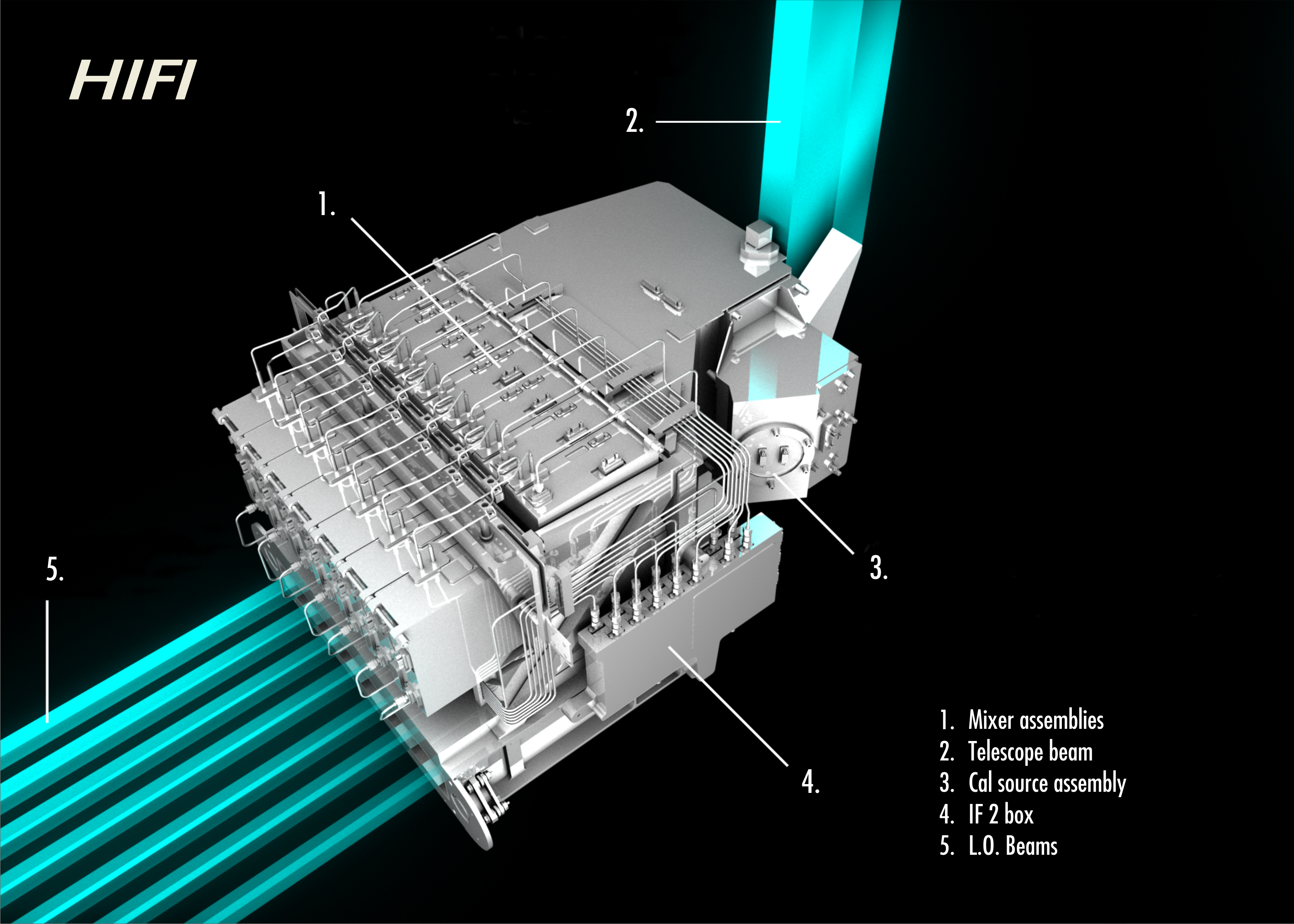
Herschel is equipped with three instruments that turn the telescope from a mere light-collector into powerful infrared eyes.

Gambar terkait

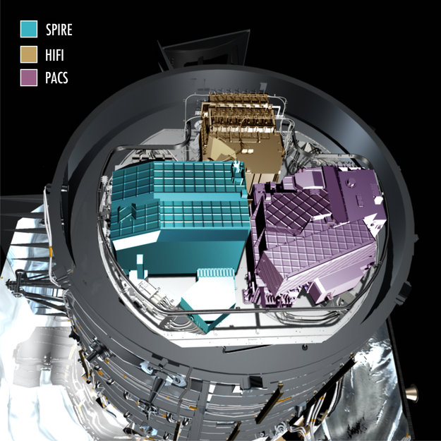
HIFI, a high-resolution spectrometer, is designed to observe unexploited wavelengths. With its high spectral resolution –– the highest ever in the range of wavelengths it covers –– HIFI will observe an unprecedented level of detail: it will be able to observe and identify individual molecular species in the enormity of space, and study their motion, temperature, and other physical properties. This is fundamental to the study of comets, planetary atmospheres, star formation and the development of distant and nearby galaxies.
HIFI can produce high-resolution spectra of thousands of wavelengths simultaneously. It covers two bands (157–212 microns and 240–625 microns), and uses superconducting mixers as detectors. It was designed and built by a nationally-funded consortium led by SRON Netherlands Institute for Space Research (Groningen, the Netherlands). The consortium includes institutes from France, Germany, USA, Canada, Ireland, Italy, Poland, Russia, Spain, Sweden, Switzerland and Taiwan.

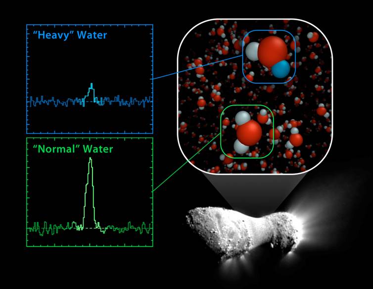
reviews amplifier electronics in space :

NASA is developing a first-ever robo mission to visit a large near-Earth asteroid, collect a multi-ton boulder from its surface, and redirect it into a stable orbit around the moon. Once it's there, astronauts will explore it and return with samples in the 2020s. This Asteroid Redirect Robo Mission (ARRM) is part of NASA's plan to advance the new technologies and spaceflight experience needed for a human mission to the Martian system in the 2030s.
Led by JPL, the mission is an integral part of NASA's plans for future human exploration, including Mars. Following proposed launch in late 2021, the spacecraft will rendezvous with and map a near-Earth asteroid, then locate and extract a large boulder. The spacecraft will demonstrate a planetary defense concept by using an enhanced gravity tractor to very slightly deflect the asteroid's orbit. The spacecraft will then maneuver the boulder into orbit around Earth's moon, where an astronaut crew in an Orion vehicle will dock to the ARRM spacecraft and conduct two spacewalks over a five-day period. The ARRM mission is enabled by significant technology advancements in low-thrust mission design, solar electric propulsion, proximity operations and roboics.
Hasil gambar untuk foto hifi satellite

Selasa, 21 Maret 2017

High - Fidelity Analog amplifier and then Digital Amplifier and processing sigma , delta , quantization processing amplifier so do Amplifier electronics in space AMNIMARJESLOW AL DO FOUR DO AL ONE LJBUSAF thankyume orbit

Listening tests

Semblance of realism

Modularity

Modern equipment

Sound recording and reproduction

Phonautograph

Phonograph

Phonograph cylinder

Disc phonograph

Electrical recording

Other recording formats

Magnetic tape

Stereo and hi-fi

1950s to 1980s

Audio components

Digital recording

Software

Legal status

UK

X . II

Frequency response

Estimation and plotting

Nonlinear frequency response

Applications

table 21032 H UPC SpecificationsValue absolute magnitude (maximum) (Ta = 25 ° C)Vcc = 18 V (rating: 8 -17 V)PT = 270 mW (Ta = 75oC)Topt = -20 + 75oC s.dS.d Tstg = -40 + 125oCOperating characteristics: Vcc = 13.2 V, RL = 10 KW, f = 1 kHz, Ta = 25oC

table 3Specifications TA 7230 PVCC = 4.5 s.d 20 VOperating conditions: VCC = 14 V, RL = 8 W, Rg = 600 W, f = 1 kHz, Ta = 25oC

Digital signal processor

Overview

Architecture

Software architecture

Instruction sets

Data instructions

Program flow

Hardware architecture

Memory architecture

Addressing and virtual memory

Modern DSPs

A Digital Amplifier Works

Hi-Fi Analog Amplifiers

Digital Amplification

Differences in Pulse-Width and Pulse-Code Modulation

Different Forms of Class D Amplification

Feedback Networks

Pros and Cons of ICE and IR Digital Amplifiers

Class-D amplifier

as like as digital amplifier

Block diagram of a basic switching or PWM (class-D) amplifier Note: For Clarity, Signal Periods are not shown to scale

Basic operation

Terminology

Signal modulation

Design challenges

Switching speed

Electromagnetic interference

Power supply design

Error control

Advantages

Uses

Class-T amplifier

Delta-sigma modulation

Motivation

Why convert an analog signal into a stream of pulses?

Why delta-sigma modulation?

Why the delta-sigma analog to digital conversion?

Analog to digital conversion

Description

Analysis

Practical Implementation

Remarks

Digital to analog conversion

Discussion

Relationship to Δ-modulation

Principle

Variations

2nd order and higher order modulator

3-level and higher quantizer

Decimation structures

Quantization theory formulas

Oversampling

table 2
1032 H UPC Specifications
Value absolute magnitude (maximum) (Ta = 25 ° C)
Vcc = 18 V (rating: 8 -17 V)
PT = 270 mW (Ta = 75oC)
Topt = -20 + 75oC s.d
S.d Tstg = -40 + 125oC
Operating characteristics: Vcc = 13.2 V, RL = 10 KW, f = 1 kHz, Ta = 25oC

table 3

Specifications TA 7230 P
VCC = 4.5 s.d 20 V
Operating conditions: VCC = 14 V, RL = 8 W, Rg = 600 W, f = 1 kHz, Ta = 25oC