Automatic control glance with
Fiber optic sensors for automation, medical, and robo


X . I PID / PITa and digital control efficiencies
Most proportional - integral - derivative (PID) applications use digital controllers, though some still use analog. Digital control can offer additional process control system efficiencies. digital controller has several advantages over analog controller to a proportional-integral-derivative (PID) applications. maybe we can explain how digital controls may offer extra efficiency of the process control system by answering five questions like the following:
Digital PID controller
I . maria: For PID applications, about how many analog controls are still in place or used?
anselo: By looking around the plants where we have control of the project and ask some customers, we would say there is less than 5% analog controllers on crop production today.
II . maria : What are the main advantages of using digital controllers over analog in PID applications?
anselo: There are many useful options in digital controllers that are unavailable in analog controllers, such as variable tuning; selectable PID structure [P and D on process variable (PV) or error] and form; gap control; error squared; tuning algorithms; accurate tuning settings; and others.
III . maria: Are there PID applications where analog has advantages over digital?
anselo: I have heard that a digital control controller must have input to output response time less than 100 milliseconds to match the speed of an analog controller. So, for loops that require a very fast response, the analog controller is faster than most digital controllers.
IIII . maria: When transitioning from analog to digital PID - type controllers, what are the special considerations, if any, for selection, setup, operation, optimization, or modifications over time?
anselo: The first step is to make sure you PROPERLY convert the current tuning in the analog controller to the digital controller.
Also, ensure you don't configure a lot of new alarms just because it is easy to do so.
Finally, investigate the new features of the digital controller to find better ways to duplicate or improve previous functionality.
IIIII . maria: beyond performance, what are some other advantages of digital controllers for PID applications?
anselo: Other advantages include ease of collecting data from the controller and easier troubleshooting the controller action.
system PID / Pita maria and anselo ; Understanding PID control and loop tuning fundamentals
 controller computes its output CO(t) by multiplying the sum of the proportional, integral, and derivative terms by the controller gain P. The proportional term is the difference between the desired setpoint SP and the measured process variable PV(t) at time t. The integral term is the sum of all past errors multiplied by the inverse integral time 1/TI. The derivative term is the rate at which the error is currently changing multiplied by the derivative time TD. Courtesy: Control Engineering")
PID loop tuning may not be a hard science, but it’s not magic either. Here are some tuning tips that work. A "control loop" is a feedback mechanism that attempts to correct discrepancies between a measured process variable and the desired setpoint. A special-purpose computer known as the "controller" applies the necessary corrective efforts via an actuator that can drive the process variable up or down. A home furnace uses a basic feedback controller to turn the heat up or down if the temperature measured by the thermostat is too low or too high.
For industrial applications, a proportional-integral-derivative (PID) controller tracks the error between the process variable and the setpoint, the integral of recent errors, and the derivative of the error signal. It computes its next corrective effort from a weighted sum of those three terms, then applies the results to the process, and awaits the next measurement. It repeats this measure-decide-actuate loop until the error is eliminated.
PID basics
A PID controller using the ideal or International Society of Automation (ISA) standard form of the PID algorithm computes its output CO(t) according to the formula shown in Figure ; PV(t) is the process variable measured at time t, and the error e(t) is the difference between the process variable and the setpoint. The PID formula weights the proportional term by a factor of P, the integral term by a factor of P/TI, and the derivative term by a factor of P.TD where P is the controller gain, TI is the integral time, and TD is the derivative time.
That terminology bears some explaining. "Gain" refers to the percentage by which the error signal will gain or lose strength as it passes through the controller en route to becoming part of the controller's output. A PID controller with a high gain will tend to generate particularly aggressive corrective efforts.
The "integral time" refers to a hypothetical sequence of events where the error starts at zero, then abruptly jumps to a fixed value. Such an error would cause an instantaneous response from the controller's proportional term and a response from the integral term that starts at zero and increases steadily. The time required for the integral term to catch up to the unchanging proportional term is the integral time TI. A PID controller with a long integral time is more heavily weighted toward proportional action than integral action.
Similarly, the "derivative time" TD is a measure of the relative influence of the derivative term in the PID formula. If the error were to start at zero and begin increasing at a fixed rate, the proportional term would start at zero, while the derivative term assumes a fixed value. The proportional term would then increase steadily until it catches up with the derivative term at the end of the derivative time. A PID controller with a long derivative time is more heavily weighted toward derivative action than proportional action.
Historical note
The first feedback controllers included just the proportional term. For mathematical reasons that only became apparent later on, a P-only controller tends to drive the error downward to a small, but non-zero, value and then quit. Operators observing this phenomenon would manually increase the controller's output until the last vestiges of the error were eliminated. They called this operation "resetting" the controller.
When the integral term was introduced, operators observed that it would tend to perform the reset operation automatically. That is, the controller would augment its proportional action just enough to eliminate the error entirely. Hence, integral action was originally called "automatic reset" and remains labeled that way on some PID controllers to this day. The derivative term was invented shortly thereafter and was described, accurately enough, as "rate control."
Tricky business
Loop tuning is the art of selecting values for the tuning parameters P, TI, and TD so that the controller will be able to eliminate an error quickly without causing the process variable to fluctuate excessively. That's easier said than done.
Consider a car's cruise controller, for example. It can accelerate the car to a desired cruising speed, but not instantaneously. The car's inertia causes a delay between the time that the controller engages the accelerator and the time that the car's speed reaches the setpoint. How well a PID controller performs depends in large part on such lags.
Suppose an overloaded car with an undersized engine suddenly starts up a steep hill. The ensuing error between the car's actual and desired speeds would cause the controller's derivative and proportional actions to kick in immediately. The controller would begin to accelerate the car, but only as fast as the lag allows.
After a while, the integral action would also begin to contribute to the controller's output and eventually come to dominate it because the error decreases so slowly when the lag time is long, and a sustained error is what drives the integral action. But exactly when that would happen and how dominant the integral action would become thereafter would depend on the severity of the lag and the relative sizes of the controller's integral and derivative times.
This simple example demonstrates a fundamental principle of PID tuning. The best choice for each of the tuning parameters P, TI, and TD depends on the values of the other two as well as the behavior of the controlled process. Furthermore, modifying the tuning of any one term affects the performance of the others because the modified controller affects the process, and the process in turn affects the controller.
 reveal the process’ dead time d (the time between points 1 and 2), time constant T (the time between points 2 and 4), and gain K (the distance between points 3 and 4 divided by B). Courtesy: Control Engineering") How can a control engineer designing a PID loop determine the values for P, TI, and TD
that will work best for a particular application? John G. Ziegler and
Nathaniel B. Nichols of Taylor Instruments (now part of ABB) addressed
that question in 1942 when they published two loop tuning techniques
that remain popular to this day.
How can a control engineer designing a PID loop determine the values for P, TI, and TD
that will work best for a particular application? John G. Ziegler and
Nathaniel B. Nichols of Taylor Instruments (now part of ABB) addressed
that question in 1942 when they published two loop tuning techniques
that remain popular to this day.
Their open loop technique is based on the results of a bump or step test for which the controller is taken offline and manually forced to increase its output abruptly. A strip chart of the process variable's subsequent trajectory is known as the "reaction curve" (see Figure 2).
A sloped line drawn tangent to the reaction curve at its steepest point shows how fast the process reacted to the step change in the controller's output. The inverse of this line's slope is the process time constant T, which measures the severity of the lag.
The reaction curve also shows how long it took for the process to demonstrate its initial reaction to the step (the dead time d) and how much the process variable increased relative to the size of the step (the process gain K). By trial-and-error, Ziegler and Nichols determined that the best settings for the tuning parameters P, TI, and TD could be computed from T, d, and K as shown by the equation:

After these parameter settings have been loaded into the PID formula and the controller returned to automatic mode, the controller should be able to eliminate future errors without causing the process variable to fluctuate excessively.
Ziegler and Nichols also described a closed loop tuning technique that is conducted with the controller in automatic mode, but with the integral and derivative actions shut off. The controller gain is increased until even the slightest error causes a sustained oscillation in the process variable (see Figure 3).
The smallest controller gain that can cause such an oscillation is called the "ultimate gain" Pu. The period of those oscillations is called the "ultimate period" Tu. The appropriate tuning parameters can be computed from these two values according to the following rules:

, forcing the process variable into sustained oscillations with a period known as the ultimate period Tu. These two values define a process’ behavior sufficiently to allow the controller to be tuned to eliminate errors with only a few oscillations. Courtesy: Control Engineering")
Caveats
Unfortunately, PID loop tuning isn't really that simple. Different PID controllers use different versions of the PID formula, and each must be tuned according to the appropriate set of rules. The rules also change when:
- The derivative and/or the integral actions are disabled.
- The process itself is inherently oscillatory.
- The process behaves as if it contains its own integral term (as is the case with level control).
- The dead time d is very small or significantly larger than the time constant T.
That's where loop tuning becomes an art. It takes more than a little experience and sometimes a lot of luck to come up with just the right combination of P, TI, and TD.
MORE ADVICE
Key concepts
A PID controller with a high gain tends to generate particularly aggressive corrective efforts.
Loop tuning is the art of selecting values for tuning parameters that enable the controller to eliminate the error quickly without causing excessive process variable fluctuations.
Different PID controllers use different versions of the PID formula, and each must be tuned according to the appropriate set of rules.
________________________________________________________________________________
Fixing PID
Proportional-integral-derivative controllers may be ubiquitous, but they’re not perfect.
Although the PID algorithm was first applied to a feedback control problem more than a century ago and has served as the de facto standard for process control since the 1940s, PID loops have seen a number of improvements over the years. Mechanical PID mechanisms have been supplanted in turn by pneumatic, electronic, and computer-based devices; and the PID calculation itself has been tweaked to provide tighter control.
Integral action or automatic reset was the first fix introduced to improve the performance of feedback controllers back when they were equipped with only proportional action. A basic “P-only” controller applies a corrective effort to the process in proportion to the difference or error between the desired setpoint and the current process variable measurement.
When the setpoint goes up or the process variable goes down, the error between them grows in the positive direction, causing a P-only controller to respond with a positive control effort that drives the process variable back up towards the setpoint. In the converse case, the error grows in the negative direction and the controller responds with a negative control effort that drives the process variable back down.

 In
this simple example of a generic control loop, a proportional-only
controller with a gain of 2 drives a process with a steady-state gain of
3. That is, the controller amplifies the error by a factor of 2 to
produce the control effort, and the process multiplies the control
effort by a factor of 3 (and adds a few transient oscillations) to
produce the process variable. If the setpoint is 70%, the process
variable will end up at 60% after the transients die out. The error
remains nonzero, yet the controller stops trying to reduce it any
further.
In
this simple example of a generic control loop, a proportional-only
controller with a gain of 2 drives a process with a steady-state gain of
3. That is, the controller amplifies the error by a factor of 2 to
produce the control effort, and the process multiplies the control
effort by a factor of 3 (and adds a few transient oscillations) to
produce the process variable. If the setpoint is 70%, the process
variable will end up at 60% after the transients die out. The error
remains nonzero, yet the controller stops trying to reduce it any
further.
Integral action operating in parallel with proportional action eliminates that steady-state error. It increases the control effort in proportion to the running total or integral of all the previous errors and continues to grow so long as any error remains. As a result, a proportional-plus-integral or “PI” controller never gives up. It continues to apply an ever-increasing control effort until the process variable reaches the setpoint.
Unfortunately, the introduction of integral action causes other problems that require their own fixes. Arguably the most significant is an increased risk of closed-loop instability where the integral action’s persistence does more harm than good. It can grow so large that it forces the process variable to overshoot the setpoint.
If the controlled process happens to be particularly sensitive to the controller’s efforts, that overshoot will cause an even larger error in the opposite direction. The controller will eventually change course in an effort to eliminate the new error but will end up driving the process variable back the other way, ending up even further from the setpoint. Eventually, the controller will start oscillating from fully on to fully off in a vain effort to reach a steady state.
The simplest solution to this problem is to reduce the amplification factor or gain by which the controller multiplies the integrated error to generate the integral action. On the other hand, reducing the integral gain risks increasing the time required for the closed-loop system to reach a steady state with zero error. Hundreds of analytical and heuristic techniques have been developed over the years to determine values for the integral and proportional gains that are just right for a particular application.
Reset windup
Integral action can also cause reset windup when the actuator is too small to implement an especially large control effort requested by the controller. That can happen when a burner isn’t large enough to supply the necessary heat, a valve is too small to generate a high enough flow rate, or a pump reaches its maximum speed. The actuator is said to be saturated at some limiting value—either its maximum or minimum output.
When actuator saturation prevents the process variable from rising any further, the controller continues to see positive errors between the setpoint and the process variable. The integrated error continues to rise, and the integral action continues to call for an increasingly aggressive control effort. However, the actuator remains stuck at its maximum output, unable to affect the process any further, so the process variable doesn’t get any closer to the setpoint.
An operator can try to fix the problem by reducing the setpoint back into the range that the actuator is capable of achieving, but the controller will not respond because of the enormous value that the total integrated error will have achieved during the time that the actuator was saturated fully on. That total will remain very large for a very long time, no matter what the current value of the error happens to be. As a result, the integral action will remain very high, and the controller will keep pushing the actuator against its upper limit.
Fortunately, the error will turn negative if the operator drops the setpoint low enough, so the total integrated error will eventually start to fall. Still, a long series of negative errors will be required to cancel the long series of positive errors that had been accumulating in the integrator’s running total. Until that happens, the integral action will remain large enough to continue saturating the actuator, no matter what the simultaneous proportional action is calling for. See the “Reset windup” graphic.
Several techniques have been devised to protect against reset windup. The obvious solution is to replace the undersized actuator with a larger one capable of actually driving the process variable all the way to the setpoint or selecting setpoints that the existing actuator can actually reach. Otherwise, the integrator can simply be turned off when the actuator saturates.
 In
this example, the operator has tried to increase the setpoint to a
value higher than the actuator is capable of achieving. After observing
that the controller has been unable to drive the process variable that
high, the operator returns the setpoint to a lower value. Note that the
controller does not begin to lower its control effort until well after
the setpoint has been lowered because the integral action has grown very
large during the controller’s futile attempt to reach the higher
setpoint. Instead, the controller continues to call for a maximum
control effort even though the error has turned negative. The control
effort does not begin to drop until the negative errors following the
setpoint change have persisted as long as the positive errors had
persisted prior to the setpoint change (or more precisely, until the
integral of the negative errors reaches the same magnitude as the
integral of the positive errors).
In
this example, the operator has tried to increase the setpoint to a
value higher than the actuator is capable of achieving. After observing
that the controller has been unable to drive the process variable that
high, the operator returns the setpoint to a lower value. Note that the
controller does not begin to lower its control effort until well after
the setpoint has been lowered because the integral action has grown very
large during the controller’s futile attempt to reach the higher
setpoint. Instead, the controller continues to call for a maximum
control effort even though the error has turned negative. The control
effort does not begin to drop until the negative errors following the
setpoint change have persisted as long as the positive errors had
persisted prior to the setpoint change (or more precisely, until the
integral of the negative errors reaches the same magnitude as the
integral of the positive errors).
 In
this case, the operator has repeated the same sequence of setpoint
moves, but this time using a PID controller equipped with reset windup
protection. Extra logic added to the PID algorithm shuts off the
controller’s integrator when the actuator hits its upper limit. The
process variable still can’t reach the higher setpoint, but the
controller’s integral action doesn’t wind up during the attempt. That
allows the controller to respond immediately when the setpoint is
lowered.
In
this case, the operator has repeated the same sequence of setpoint
moves, but this time using a PID controller equipped with reset windup
protection. Extra logic added to the PID algorithm shuts off the
controller’s integrator when the actuator hits its upper limit. The
process variable still can’t reach the higher setpoint, but the
controller’s integral action doesn’t wind up during the attempt. That
allows the controller to respond immediately when the setpoint is
lowered.
Pre-loading
Reset windup also occurs when the actuator is turned off but the controller isn’t. In a cascade controller, for example, the outer-loop controller will see no response to its control efforts while the inner loop is in manual mode. If the outer-loop controller is left operating during that interval, its integral action will “wind up” as the error remains constant.
Similarly, when the burner, valve, or pump is shut down between cycles of a batching operation, the process variable is prevented from getting any closer to the setpoint, again leading to windup. That’s not a problem while the actuator remains off, but as soon the actuator is reactivated at the beginning of the next batch, the controller will immediately call for a 100% control effort and saturate the actuator.
The obvious solution to this problem is to turn off the controller’s integrator whenever the actuator is turned off or to eliminate the error artificially by adjusting the setpoint to whatever value the process variable takes between batches. But there’s another approach that not only prevents reset windup between batches but actually improves the controller’s performance during the next batch.
Pre-loading freezes the output of the controller’s integrator between batches so that the integral action starts the next batch with the total integrated error that it had accumulated as of the end of the previous batch. This technique assumes that the controller is eventually going to need the same amount of integral action to reach the same steady state as in the previous batch, so there’s no point in starting the integrated error at zero. With pre-loading, the integral action essentially picks up right where it left off at the end of the previous batch, thereby shortening the time required to achieve a steady state in the next batch.
Pre-loading works best if each successive batch is more-or-less identical to its predecessor so that the controller is attempting to achieve the same setpoint under the same load conditions every time. But even if the batches aren’t identical, it is sometimes possible to use a mathematical model of the process to predict what level of integral action is eventually going to be required to achieve a steady state. The required integrated error can then be deduced and pre-loaded into the controller’s integrator at the start of each batch. This approach will also work for a continuous process if it can be modeled prior to the initial start-up.
Bumpless transfer
One potential drawback to pre-loading is the abrupt change it can cause in the actuator’s output at the beginning of each batch. Although the actuator won’t immediately slam all the way open if pre-loading is used to prevent reset windup, it will try to start the next batch at or near the position it was in at the end of the previous batch. If that causes an abrupt change that is likely to damage the actuator, the controller’s integrator can be ramped up gradually to its pre-load value.
A similar problem can occur when a controller is switched from automatic to manual mode and back again. If an operator manually modifies the control effort during that interval, the controller will abruptly switch the control effort to whatever the PID algorithm is calling for at the time automatic mode is resumed.
Bumpless transfer solves this problem by artificially pre-loading the integrator with whatever value is required to restart automatic operations without changing the control effort from wherever the operator left it. The controller will still have to make adjustments if the operator’s actions, changes in the process variable, or changes in the setpoint have created an error while the controller was in manual mode, but less of a “bump” will result when the controller is “transferred” back to automatic mode.
Still more windup problems
All of these windup-related problems are compounded by deadtime—the interval required for the process variable to change following a change in the control effort. Deadtime typically occurs when the process variable sensor is located too far downstream from the actuator. No matter how hard the controller works, it cannot begin to reduce an error between the process variable and the setpoint until the material that the actuator has modified reaches the sensor.
As the controller is waiting for its efforts to take effect, the process variable and the error will remain fixed, causing the integral action to wind up just as if the actuator were saturated or turned off. The most common fix to this problem is to de-tune the controller; that is, reduce the integral gain to reduce the maximum integral action caused by windup.
The same effect can be achieved by equipping the integral action with its own deadtime so that windup does not begin until at least some of the process deadtime has elapsed. This in turn lowers the total integrated error that the controller can accumulate during the interval that the error is fixed.
Deadtime-induced windup can also be ameliorated by making the integral action intermittent. Let the proportional action do all the work until the process variable has settled somewhere close to the setpoint, then turn on the integral action only long enough to eliminate the remaining steady-state error. This approach not only delays the onset of windup, it gives the integral action only small errors to deal with, thereby reducing the maximum windup effect.
But wait, there’s more
This only scratches the surface of the many ways engineers have sought to improve control performance. The PID algorithm has also been modified to deal with velocity-limited actuators, time-varying process models, noise in the process variable measurement, excessive derivative action during setpoint changes, and more. Future installments of this series will look at the effects these problems cause and how they can be avoided.
_________________________________________________________________________________
Open- vs. closed-loop control
Automatic control operations can be described as either open-loop or closed-loop. The difference is feedback.
- The process that is to be controlled
- An instrument with a sensor that measures the condition of the process
- A transmitter that converts the measurement into an electronic signal
- A controller that reads the transmitter's signal and decides whether or not the current condition of the process is acceptable, and
- An actuator functioning as the final control element that applies a corrective effort to the process per the controller's instructions.
 In
a closed-loop control system, information flows around a feedback loop
from the process to the sensor to the transmitter to the controller to
the actuator and back to the process. This measure-decide-actuate
sequence-known as closed-loop control-repeats as often as necessary
until the desired process condition is achieved. Familiar examples
include using a thermostat controlling a furnace to maintain the
temperature in a room or cruise control to maintain the speed of a car.
In
a closed-loop control system, information flows around a feedback loop
from the process to the sensor to the transmitter to the controller to
the actuator and back to the process. This measure-decide-actuate
sequence-known as closed-loop control-repeats as often as necessary
until the desired process condition is achieved. Familiar examples
include using a thermostat controlling a furnace to maintain the
temperature in a room or cruise control to maintain the speed of a car.
But not all automatic control operations require feedback. A much larger class of control commands can be executed in an open-loop configuration without confirmation or further adjustment. Open-loop control is sufficient for predictable operations such as opening a door, starting a motor, or turning off a pump.
Continuous closed-loop control
Continuing the analysis, it is clear that all closed-loop operations are not alike. For a continuous process, a feedback loop attempts to maintain a process variable (or controlled variable) at a desired value known as the setpoint. The controller subtracts the latest measurement of the process variable from the setpoint to generate an error signal. The magnitude and duration of the error signal then determines the value of the controller's output or manipulated variable which in turn dictates the corrective efforts applied by the actuator.
For example, a car equipped with a cruise control uses a speedometer to measure and maintain the car's speed. If the car is traveling too slowly, the controller instructs the accelerator to feed more fuel to the engine. If the car is traveling too quickly, the controller lets up on the accelerator. The car is the process, the speedometer is the sensor, and the accelerator is the actuator.
The car's speed is the process variable. Other common process variables include temperatures, pressures, flow rates, and tank levels. These are all quantities that can vary constantly and can be measured at any time. Common actuators for manipulating such conditions include heating elements, valves, and dampers.
Discrete closed-loop control
For a discrete process, the variable of interest is measured only when a triggering event occurs, and the measure-decide-actuate sequence is typically executed just once for each event. For example, the human controller driving the car uses her eyes to measure ambient light levels at the beginning of each trip. If she decides that it's too dark to see well, she turns on the car's lights. No further adjustment is required until the next triggering event such as the end of the trip.
Feedback loops for discrete processes are generally much simpler than continuous control loops since discrete processes do not involve as much inertia. The driver controlling the car gets instantaneous results after turning on the lights, whereas the cruise control sees much more gradual results as the car slowly speeds up or slows down.


Inertia tends to complicate the design of a continuous control loop since a continuous controller typically needs to make a series of decisions before the results of its earlier efforts are completely evident. It has to anticipate the cumulative effects of its recent corrective efforts and plan future efforts accordingly. Waiting to see how each one turns out before trying another simply takes too long.
Open-loop control
Open-loop controllers do not use feedback per se. They apply a single control effort when so commanded and assume that the desired results will be achieved. An open-loop controller may still measure the results of its commands: Did the door actually open? Did the motor actually start? Is the pump actually off? Generally, these actions are for safety considerations rather than as part of the control sequence.
Even closed-loop feedback controllers must operate in an open-loop mode on occasion. A sensor may fail to generate the feedback signal or an operator may take over the feedback operation in order to manipulate the controller's output manually.
Operator intervention is generally required when a feedback controller proves unable to maintain stable closed-loop control. For example, a particularly aggressive pressure controller may overcompensate for a drop in line pressure. If the controller then overcompensates for its overcompensation, the pressure may end up lower than before, then higher, then even lower, then even higher, etc. The simplest way to terminate such unstable oscillations is to break the loop and regain control manually.
There are also many applications where experienced operators can make manual corrections faster than a feedback controller can. Using their knowledge of the process' past behavior, operators can manipulate the process inputs now to achieve the desired output values later. A feedback controller, on the other hand, must wait until the effects of its latest efforts are measurable before it can decide on the next appropriate control action. Predictable processes with longtime constants or excessive dead time are particularly suited for open-loop manual control.
Open- and closed-loop control combined
The principal drawback of open-loop control is a loss of accuracy. Without feedback, there is no guarantee that the control efforts applied to the process will actually have the desired effect. If speed and accuracy are both required, open-loop and closed-loop control can be applied simultaneously using a feedforward strategy. A feedforward controller uses a mathematical model of the process to make its initial control moves like an experienced operator would. It then measures the results of its open-loop efforts and makes additional corrections as necessary like a traditional feedback controller.


Feedforward is particularly useful when sensors are available to measure an impending disturbance before it hits the process. If its future effects on the process can be accurately predicted with the process model, the controller can take preemptive actions to counteract the disturbance as it occurs.
For example, if a car equipped with cruise control and radar could see a hill coming, it could begin to accelerate even before it begins to slow down. The car may not end up at the desired speed as it climbs the hill, but even that error can eventually be eliminated by the cruise controller's normal feedback control algorithm. Without the advance notice provided by the radar, the cruise controller wouldn't know that acceleration is required until the car had already slowed below the desired speed halfway up the hill.
Open- and closed-loop control in parallel
Many automatic control systems use both open- and closed-loop control in parallel. Consider, for example, a brewery that ferments and bottles beer.
Brew kettles in a modern brewery rely on continuous closed-loop control to maintain prescribed temperatures and pressures while turning water and grain into fermentable mash.
A brewery's bottling line uses both discrete closed-loop control and open-loop control to fill and cap the individual bottles.
The conditions inside the brew kettles are maintained by closed-loop controllers using feedback loops that measure the temperature and pressure, then adjust steam flow into the kettle and flow pumps to compensate for out-of-spec conditions. Open-loop control is also required for one-time operations such as starting and stopping the mixer motors or opening and closing the steam lines to the heat exchangers.
Simultaneously, finished batches of beer are bottled using open-loop and discrete closed-loop control. A proximity sensor determines that a bottle is present before filling can begin, then a valve opens to fill each bottle until a level sensor determines that the bottle is full.
In general, continuous closed-loop control applications require at least a few ancillary open-loop control operations, whereas many open-loop control applications require no feedback loops at all.
Which is which?
The differences between continuous closed-loop control, discrete closed-loop control, and open-loop control can be subtle. Here are some snippets of pseudo-code to illustrate each:
Open-loop control
IF (time_for_action = TRUE) THEN
take_action(X)
END
Discrete closed-loop control
IF (time_for_action = TRUE) THEN
measure(Y)
IF (Y = specified_condition) THEN
take_action(X)
END
END
Continuous closed-loop control
WHILE (Y <> specified_condition)
take_action(X)
measure(Y)
wait(Z)
REPEAT
In the first two cases the time for action usually means that a particular step has been reached in the control sequence. At that point, an open-loop controller would simply execute action X and proceed to the next step in the program. A discrete closed-loop controller would first measure or observe some condition Y in the process to determine if action X needs to be executed or not. Once activated, a continuous closed-loop controller is always ready for action. It takes action X, measures condition Y, waits Z seconds, then repeats the loop unless Y had reached the specified condition. In the discrete case, the specified condition is usually a discrete event such as the completion of a prior task or a change in some go/no-go decision criteria. In the continuous case, the specified condition is usually met when the measured variable reaches a desired value.
Key concepts:
- There are different types of control loops and the most critical characteristic that separates them is how they handle feedback.
- The needs of an application should be the primary reason for choosing one type or another.
- In some cases, human intervention may be more desirable than an automatic approach.
Fundamentals of integrating vs. self-regulating processes
Sometimes a process is easier to control if it “leaks.” Here’s a look at why.


An integrating process produces an output that is proportional to the running total of some input that the process has been accumulating over time. Alternately, an integrating process can accumulate a related quantity proportional to the input rather than the input itself. Either way, if the input happens to turn negative, an integrating process will start to relinquish whatever it has accumulated, thereby lowering its output.
For the water tank shown in the "Integrating process example," input is the water flowing into the tank—the net flow from all incoming streams minus outgoing streams. The output is the level of water the tank has accumulated. As long as net inflow remains positive (more incoming than outgoing), the output level will continue to increase as the tank fills up. If net inflow turns negative (more outgoing than incoming), output level will decrease as the tank drains.
Servo motors have an entirely different accumulation mechanism, but the same effects. A servo motor's input voltage generates torque, which accelerates a load around the shaft. The resulting rotation turns the load a bit more for every instant input voltage is non-zero. The load's net position results from the accumulation of all those incremental rotations, each of which is proportional to input voltage at that instant. As long as input voltage remains positive, the output position will continue to increase. If input voltage turns negative, the output position will decrease as the shaft turns backwards.
The water tank and servo motor also behave similarly in that fixing their inputs at zero will fix their outputs at whatever values they'd reached up to that point. The tank's water level will remain unchanged as long as incoming flow exactly matches outgoing flow (typically when both are zero), and the servo motor's shaft will remain in its last position as long as input voltage is neither positive nor negative.
This is a defining characteristic of all integrating processes. They can accumulate their inputs and subsequently disperse them without suffering spontaneous losses to the surrounding environment. Accumulation and dispersal rates can vary considerably from process to process, and the two rates can be different within the same process depending on the effects of friction and inertia. But once a chunk of input has been successfully added to the running total, it will stay there until a negative input removes it. That is, a drop of water that has entered the tank will remain within (or be replaced) until outflow exceeds inflow.
Losses as well as gains
Other processes can lose what they've accumulated without the benefit of a negative input. A leaky tank will lose water no matter how the inlet and outlet valves are set, and a servo motor rotating against a torsional spring will lose position whether input voltage is positive, negative, or zero.
Such processes can reach an equilibrium point where further accumulations are offset by spontaneous losses. If a tank is leaky enough, a given inflow rate will not be able to raise the output level beyond a certain height. If the spring opposing the servo motor is strong enough, it will eventually prevent the shaft from rotating any further.
These are often called non-integrating processes, though "short-term integrating" might be a more apt description. They accumulate their inputs just as integrating processes do but only until they reach an equilibrium point between input and losses, as shown in the "Non-integrating process example."

Key concepts:
- Processes have specific characteristics that affect the way in which they should be controlled.
- Understanding how a process responds to control efforts is a critical step of establishing control strategy.
Fundamentals of cascade control
Sometimes two controllers can do a better job of keeping one process variable where you want it.
When multiple sensors are available for measuring conditions in a
controlled process, a cascade control system can often perform better
than a traditional single-measurement controller. Consider, for example,
the steam-fed water heater shown in the sidebar Heating Water with
Cascade Control. In Figure A, a traditional controller is shown
measuring the temperature inside the tank and manipulating the steam
valve opening to add more or less heat as inflowing water disturbs the
tank temperature. This arrangement works well enough if the steam supply
and the steam valve are sufficiently consistent to produce another X%
change in tank temperature every time the controller calls for another
Y% change in the valve opening.
However, several factors could alter the ratio of X to Y or the time
required for the tank temperature to change after a control effort. The
pressure in the steam supply line could drop while other tanks are
drawing down the steam supply they share, in which case the controller
would have to open the valve more than Y% in order to achieve the same
X% change in tank temperature.
Or, the steam valve could start sticking as friction takes its mechanical toll over time. That would lengthen the time required for the valve to open to the extent called for by the controller and slow the rate at which the tank temperature changes in response to a given control effort.
A better way
 A
cascade control system could solve both of these problems as shown in
Figure B where a second controller has taken over responsibility for
manipulating the valve opening based on measurements from a second
sensor monitoring the steam flow rate. Instead of dictating how widely
the valve should be opened, the first controller now tells the second
controller how much heat it wants in terms of a desired steam flow rate.
A
cascade control system could solve both of these problems as shown in
Figure B where a second controller has taken over responsibility for
manipulating the valve opening based on measurements from a second
sensor monitoring the steam flow rate. Instead of dictating how widely
the valve should be opened, the first controller now tells the second
controller how much heat it wants in terms of a desired steam flow rate.
The second
controller then manipulates the valve opening until the steam is flowing at the requested rate. If that rate turns out to be insufficient to produce the desired tank temperature, the first controller can call for a higher flow rate, thereby inducing the second controller to provide more steam and more heat (or vice versa).
That may sound like a convoluted way to achieve the same result as the first controller could achieve on its own, but a cascade control system should be able to provide much faster compensation when the steam flow is disturbed. In the original single-controller arrangement, a drop in the steam supply pressure would first have to lower the tank temperature before the temperature sensor could even notice the disturbance. With the second controller and second sensor on the job, the steam flow rate can be measured and maintained much more quickly and precisely, allowing the first controller to work with the belief that whatever steam flow rate it wants it will in fact get, no matter what happens to the steam pressure.
The second controller can also shield the first controller from deteriorating valve performance. The valve might still slow down as it wears out or gums up, and the second controller might have to work harder as a result, but the first controller would be unaffected as long as the second controller is able to maintain the steam flow rate at the required level.
Without the acceleration afforded by the second controller, the first controller would see the process becoming slower and slower. It might still be able to achieve the desired tank temperature on its own, but unless a perceptive operator notices the effect and re-tunes it to be more aggressive about responding to disturbances in the tank temperature, it too would become slower and slower.
Similarly, the second controller can smooth out any quirks or nonlinearities in the valve's performance, such as an orifice that is harder to close than to open. The second controller might have to struggle a bit to achieve the desired steam flow rate, but if it can do so quickly enough, the first controller will never see the effects of the valve's quirky behavior.
Elements of cascade control
The Cascade Control Block Diagram shows a generic cascade control system with two controllers, two sensors, and one actuator acting on two processes in series. A primary or master controller generates a control effort that serves as the setpoint for a secondary or slave controller. That controller in turn uses the actuator to apply its control effort directly to the secondary process. The secondary process then generates a secondary process variable that serves as the control effort for the primary process.
The geometry of this block diagram defines an inner loop involving the secondary controller and an outer loop involving the primary controller. The inner loop functions like a traditional feedback control system with a setpoint, a process variable, and a controller acting on a process by means of an actuator. The outer loop does the same except that it uses the entire inner loop as its actuator.
In the water heater example, the tank temperature controller would be primary since it defines the setpoint that the steam flow controller is required to achieve. The water in the tank, the tank temperature, the steam, and the steam flow rate would be the primary process, the primary process variable, the secondary process, and the secondary process variable, respectively (refer to the Cascade Control Block Diagram). The valve that the steam flow controller uses to maintain the steam flow rate serves as the actuator which acts directly on the secondary process and indirectly on the primary process.
Requirements
Naturally, a cascade control system can't solve every feedback control problem, but it can prove advantageous if under the right circumstances:
- The inner loop has influence over the outer loop. The actions of the secondary controller must affect the primary process variable in a predictable and repeatable way or else the primary controller will have no mechanism for influencing its own process.
- The inner loop is faster than the outer loop. The secondary process must react to the secondary controller's efforts at least three or four times faster than the primary process reacts to the primary controller. This allows the secondary controller enough time to compensate for inner loop disturbances before they can affect the primary process.
- The inner loop disturbances are less severe than the outer loop disturbances. Otherwise, the secondary controller will be constantly correcting for disturbances to the secondary process and unable to apply consistent corrective efforts to the primary process.
Cascade control block diagram
A cascade control system reacts to physical phenomena shown in blue and process data shown in green.

In the water heater example:
- Setpoint - temperature desired for the water in the tank
- Primary controller (master) - measures water temperature in the tank and asks the secondary controller for more or less heat
- Secondary controller (slave) - measures and maintains steam flow rate directly
- Actuator - steam flow valve
- Secondary process - steam in the supply line
- Inner loop disturbances - fluctuations in steam supply pressure
- Primary process - water in the tank
- Outer loop disturbances - fluctuations in the tank temperature due to uncontrolled ambient conditions, especially fluctuations in the inflow temperature
- Secondary process variable - steam flow rate
- Primary process variable - tank water temperature
Cascade control can also have its drawbacks. Most notably, the extra sensor and controller tend to increase the overall equipment costs. Cascade control systems are also more complex than single-measurement controllers, requiring twice as much tuning. Then again, the tuning procedure is fairly straightforward: tune the secondary controller first, then the primary controller using the same tuning tools applicable to single-measurement controllers.
However, if the inner loop tuning is too aggressive and the two processes operate on similar time scales, the two controllers might compete with each other to the point of driving the closed-loop system unstable. Fortunately, this is unlikely if the inner loop is inherently faster than the outer loop or the tuning forces it to be.
And it's not always clear when cascade control will be worth the extra effort and expense. There are several classic examples that typically benefit from cascade control-often involving a flow rate as the secondary process variable-but it's usually easier to predict when a cascade control system won't help than to predict when it will.
Key concepts:
- When more than one element can affect a single process variable, treating each separately can make the process easier to control.
- One process variable that depends on more than one measurement might need more than one controller.
________________________________________________________________________________
Back to Basics: Closed-loop stability
Stability is how a control loop reduces errors between the measured process variable and its desired value or setpoint.
For the purposes of feedback control, stability refers to a control loop’s ability to reduce errors between the measured process variable and its desired value or setpoint. A stable control loop will manipulate the process so as to bring the process variable closer to the setpoint, whereas an unstable control loop will maintain or even widen the gap between them.
With the exception of explosive devices that depend on self-sustained reactions to increase the temperature and pressure of a process exponentially, feedback loops are generally designed to be stable so that the process variable will eventually achieve a constant steady state after a setpoint change or a disturbance to the process.Unfortunately, some control loops don’t turn out that way. The problem is often a matter of inertia – a process’s tendency to continue moving in the same direction after the controller has tried to reverse course.
Consider, for example, the child’s toy shown in the first figure. It consists of a
weight hanging from a vertical spring that the human controller can raise or lower by tugging on the spring’s handle. If the controller’s goal is to position the weight at a specified height above the floor, it would be a simple matter to slowly raise the
handle until the height measurement matches the desired setpoint.

Doing so would certainly achieve the desired objective, but if this were an industrial positioning system, the inordinate amount of time required to move the weight slowly to its final height would degrade the performance of any process that depends on the weight’s position. The longer the weight remains above or below the setpoint, the poorer the performance.
Moving the weight faster would address the time-out-of-position problem, but moving it too quickly could make matters worse. The weight’s inertia might cause it to move past the setpoint even after the controller has observed the impending overshoot and begun pushing in the opposite direction. And if the controller’s attempt to reverse course is also too aggressive, the weight will overshoot the other way.Fortunately, each successive overshoot will typically be smaller than the last so that the weight will eventually reach the desired height after bouncing around a bit. But as anyone who has ever played with such a toy knows, the faster the controller moves the handle, the longer those oscillations will be sustained. And at one particular speed corresponding to the resonant frequency of the weight-and-spring process, each successive overshoot will have the same magnitude as its predecessor and the oscillations will continue until the controller gives up.
But if the controller were to become even more aggressive, those oscillations would grow in magnitude until the spring reaches its maximum distention or breaks. Such an unstable control loop might be amusing for a child playing with a toy spring, but it would be disastrous for a commercial positioning system or any other application of closed-loop feedback.
One solution to this problem would be to limit the controller’s aggressiveness by equipping it with a speed-sensitive damper such as a dashpot or a shock absorber as shown in the second figure. Such a device would resist the controller’s movements more and more as the controller tries to move faster and faster. The
derivative term in a PID controller serves the same function, though too much derivative damping can actually make matters worse.

__________________________________________________________________________________
Disturbance-Rejection vs. Setpoint-Tracking Controllers
Designing a feedback control loop starts with understanding its objective as well as the process’s behavior.
The principal objective of a feedback controller is typically either disturbance rejection or setpoint tracking. A controller designed to reject disturbances will take action to force the process variable back toward the desired setpoint whenever a disturbance or load on the process causes a deviation.
A car’s cruise controller, for example, will throttle up the engine whenever it detects a drop in the car’s speed during an uphill climb. It will continue working to reject or overcome the extra load on the car until the car is once again moving as fast as the driver originally specified. Disturbance-rejection controllers are best suited for applications where the setpoint is constant and the process variable is required to stay close to it.
 or by affecting the process variable directly. Either way, the controller then measures the resulting process variable and repeats its closed-loop operations until it has forced the error to zero. All feedback control loops work this way, but the ideal configuration for a particular application depends on whether errors are caused mostly by disturbances or by setpoint changes and the relative speed of each. SOURCE: Control Engineering")
In contrast, a setpoint-tracking controller is appropriate when the setpoint is expected to change frequently and the controller is required to raise or lower the process variable accordingly. A luxury car equipped with an automatic temperature controller will track a changing setpoint by adjusting the heater’s output whenever a new driver calls for a new interior temperature.
Disturbance-rejection and setpoint-tracking controllers can each do the job of the other (a cruise controller can increase the car’s speed when the driver wants to go faster, and the car’s temperature controller can cut back the heating when the sun comes out), but optimal performance generally requires that a controller be designed or tuned for one role or the other. To see why, consider the feedback loop shown in the Control Loop diagram and the effects of an abrupt disturbance to the process or an abrupt change in the process variable’s setpoint.
Open-loop operations
First, suppose that the feedback path is disabled so that the controller is operating in open-loop mode. After a disturbance, the process variable will begin to change according to the magnitude of the load and the physical characteristics of the process. In the cruise control example, the sudden resistance added by the hill will start to decelerate the car according to the hill’s steepness and the car’s inertia.

Note that an open-loop controller doesn’t actually play any role in determining how the process reacts to a disturbance, so the controller’s tuning is irrelevant when feedback is disabled. In contrast, a setpoint change will pass through both the controller and the process, even without any feedback. See the Open-Loop Operations diagram.
As a result, the mathematical inertia of the controller combines with the physical inertia of the process to make the process’s response to a setpoint change slower than its response to an abrupt disturbance. This is especially true when the controller is equipped with integral action. The I component of a PID controller tends to filter or average-out the effects of a setpoint change by introducing a time lag that limits the rate at which the resulting control effort can change.

In the car temperature control example, this phenomenon is evident when the controller starts turning up the heat upon receiving the driver’s request for a warmer interior. The car’s heater will in turn begin to raise the car’s temperature at a rate that depends on how aggressively the controller is tuned and how quickly the interior temperature reacts to the heater’s efforts. A direct disturbance such as a burst of sunshine would typically raise the car’s temperature at a much faster rate because the effects of the disturbance would not depend on the controller ramping up first.
Closed-loop operations
Of course an open-loop controller can’t really reject disturbances nor track setpoint changes without feedback, so it makes sense to ask, “What happens to that extra setpoint response time when the feedback is enabled?” Usually, nothing. Unless the controller happens to be equipped with setpoint filtering, the setpoint response will remain slower than the disturbance response by exactly the same amount as in the open-loop case. See the Closed-Loop Operations diagram.
, the original control loop diagram can be rearranged mathematically to show how disturbances affect the process variable. Disturbances pass through a modified process that is mathematically equivalent to the original process being driven by a feedback signal passing through the controller. SOURCE: Control Engineering")
But since that difference in response times is attributable entirely to the time lag of the controller, one might wonder if it would still be possible to design a setpoint-tracking controller that is just as fast as its disturbance-rejection counterpart by tuning it to respond instantaneously to a setpoint change.
That won’t work either. Eliminating the controller’s time lag would require disabling its integral action, and that would prevent the process variable from ever reaching the setpoint. For more on this steady-state offset phenomenon, see “The Three Faces of PID ;

On the other hand, the controller’s mathematical inertia can be minimized without completely defeating its ability to eliminate errors between the process variable and the setpoint. A fast setpoint-tracking controller would require particularly aggressive tuning, but that shouldn’t be a problem so long as the controller never needs to reject a disturbance. But if an unexpected load ever does disturb the process abruptly, a setpoint-tracking controller will tend to overreact and cause the process variable to oscillate unnecessarily.

Conversely, a controller tuned to reject abrupt disturbances will typically be relatively slow about implementing a setpoint change. Fortunately, a typical feedback control loop in an industrial application will operate for extended periods at a constant setpoint, so the only time that a disturbance-rejection controller normally experiences a delay because of a setpoint change is at start-up.
Caveats
Unfortunately, that’s not the end of the disturbance-rejection vs. setpoint-tracking story. To this point we have assumed that the process is subject to abrupt disturbances such as when a car with cruise control suddenly encounters a steep hill. Many if not most feedback control applications involve much less dramatic disturbances—rolling hills rather than steep inclines, for example.
When the physical properties of the process limit the rate at which disturbances can affect the process variable, the disturbance response will sometimes be slower than the setpoint response, not faster. In such cases, more aggressive tuning would be appropriate for a disturbance-rejection controller than for its setpoint-tracking counterpart. The key is determining which scenario applies to the process at hand and which objective the controller is required to achieve.
___________________________________________________________________________________
Tuning PID loops for level control
One-in-four control loops are regulating level, but techniques for tuning PID controllers in these integrating processes are not widely understood.
Since the first two PID controller tuning methods were published in 1942 by J. G. Ziegler and N. B. Nichols, more than 100 additional tuning rules have been developed for self-regulating control loops (e.g., flow, temperature, pressure). In contrast, fewer than 10 tuning methods have been developed for integrating (e.g., level) process types, though roughly one-in-four industrial PID loops controls liquid level.

Applicable process types
This modified Ziegler-Nichols tuning method is intended for use with integrating processes, and level control loops (Figure ) are the most common example.
 Unlike
a self-regulating process, an integrating process will stabilize at
only one controller output, which has to be at the point of equilibrium.
If the controller output is set to a different value, the process will
increase or decrease indefinitely at a steady slope
Unlike
a self-regulating process, an integrating process will stabilize at
only one controller output, which has to be at the point of equilibrium.
If the controller output is set to a different value, the process will
increase or decrease indefinitely at a steady slope Note: This tuning method provides a fast response to disturbances in level and is therefore not suitable for tuning surge tank level control loops.
The modified Ziegler-Nichols tuning rules presented here are designed for use on a non-interactive controller algorithm with its integral time set in minutes. Dataforth's MAQ20 industrial data acquisition and control system uses this approach as do other controllers from a variety of manufacturers.
Procedure
To apply these tuning rules to an integrating process, follow these steps. The process variable and controller output must be time-trended so that measurements can be taken from them, as illustrated in Figure 3.
Step I. Do a step test
a) Make sure, as far as possible, that the uncontrolled flow in and out of the vessel is as constant as possible.
b) Put the controller in manual control mode.
c) Wait for a steady slope in the level. If the level is very volatile, wait long enough to be able to confidently draw a straight line though the general slope of the level.
d) Make a step change in the controller output. Try to make the step change 5% to 10% in size, if the process can tolerate it.
e) Wait for the level to change its slope into a new direction. If the level is volatile, wait long enough to be able to confidently draw a straight line though the general slope of the level.
f) Restore the level to an acceptable operating point and place the controller back into automatic control mode.
Step II. Determine process characteristics
 Based on the example shown in Figure 3:
a) Draw a line (Slope 1) through the initial slope, and extend it to the right as shown in Figure 3.
b) Draw a line (Slope 2) through the final slope, and extend it to the left to intersect Slope 1.
c) Measure the time between the beginning of the change in controller output and the intersection between Slope 1 and Slope 2. This is the process dead time (td), the first parameter required for tuning the controller.
d) If td was measured in seconds, divide it by 60 to convert it to minutes. As mentioned earlier, the calculations here are based on the integral time in minutes, so all time measurements should be in minutes.
e) Pick any two points (PV1 and PV2) on Slope 1, located conveniently far from each other to make accurate measurements.
f) Pick any two points (PV3 and PV4) on Slope 2, located conveniently far from each other to make accurate measurements.
g) Calculate the difference in the two slopes (DS) as follows:
DS = (PV4 - PV3) / T2 - (PV2 - PV1) / T1
Note: If T1 and T2 measurements were made in seconds, divide them by 60 to convert them to minutes.
h) If the PV is not ranged 0%-100%, convert DS to a percentage of the range as follows:
DS% = 100 × DS / (PV range max - PV range min)
i) Calculate the process integration rate (ri), which is the second parameter needed for tuning the controller:
ri = DS [in %] / dCO [in %]
Step III. Repeat
Perform steps 1 and 2 at least three more times to obtain good average values for the process characteristics td and ri.
Step IIII. Calculate tuning constants
Using the equations below, calculate your tuning constants. Both PI and PID calculations are provided since some users will select the former based on the slow-moving nature of many level applications.
For PI Control
Controller Gain, Kc = 0.45 / (ri × td)
Integral Time, Ti = 6.67 × td
Derivative Time, Td = 0
For PID Control
Controller Gain, Kc = 0.75 / (ri × td)
Integral Time, Ti = 5 × td
Derivative Time, Td = 0.4 × td
Note that these tuning equations look different from the commonly published Ziegler-Nichols equations. The first reason is that Kc has been reduced and Ti increased by a factor of two, to make the loop more stable and less oscillatory. The second reason is that the Ziegler-Nichols equations for PID control target an interactive controller algorithm, while this approach is designed for a non-interactive algorithm such as is used in the Dataforth MAQ20 and others. (If you are using a different controller, make sure you find out which approach it uses.) The PID equations above have been adjusted to compensate for the difference.
Step IIIII . Enter the values
 Key
your calculated values into the controller, making sure the algorithm
is set to non-interactive, and put the controller back into automatic
mode.
Key
your calculated values into the controller, making sure the algorithm
is set to non-interactive, and put the controller back into automatic
mode.
Step IIIIII . Test and tune your work
Change the setpoint to test the new values and see how it responds. It might still need some additional fine-tuning to look like Figure 4. For integrating processes, Kc and Ti need to be adjusted simultaneously and in opposite directions. For example, to slow down the control loop, use Kc / 2 and Ti × 2.
With just a few modifications to the original Ziegler-Nichols tuning approach, these rules can be used to tune level control loops for both stability and fast response to setpoint changes and disturbances.
Lee Payne is CEO of Dataforth.
Key concepts:
- Modified Ziegler-Nichols tuning rules are effective for tuning level control loops.
- They are designed for use with integrating processes and on non-interactive controller algorithms.
- These rules provide loop stability as well as fast response to setpoint changes and disturbances.
_________________________________________________________________________________
Designing control: Smart sensors and data acquisition
Smart sensors enable accurate, efficient, and expansive data collection. Smart sensing solutions can preserve signal integrity in harsh industrial environments and give customers quick and easy solutions for test and measurement and other big data applications.

Traditional sensors such as thermocouples, resistance temperature detectors (RTDs), strain gages, linear variable differential transducers (LVDTs) and flowmeters measure physical parameters and provide data needed to monitor and control processes. Many of these produce low-level analog outputs that require precision signal conditioning to preserve the critical information they are gathering. Signal conditioning functions include sensor excitation, signal amplification, anti-alias filtering, low-pass and high-pass filtering, linearization, and an often overlooked but essential feature—isolation. Once signal conditioning has been performed, sensor signals can be digitized using an analog-to-digital converter and then further processed by a data acquisition system.
System on a chip
Developments in electronics are rapidly changing the way process data is collected using sensors. Microcontrollers and microprocessors have become much more sophisticated, incorporating communications interfaces, excitation sources, high-resolution analog to digital (A to D) and D to A converters, general purpose discrete I/O, fast architectures, math support, and low-power modes. Commonly called SoC, or system-on-chip, these small devices outperform the full and half-length ISA and PCI card solutions of yesterday at a much reduced cost. Microcontrollers with integrated data converters are even available in packages as small as 2 mm x 3 mm.
So what does all this mean for smart sensors and data acquisition? How are these changes in electronics technology changing the way data is acquired and used?
First, let's understand what a smart sensor is. Smart sensors analyze collected measurements, make decisions based on the physical parameter being measured, and most importantly, are able to communicate. Local computational power enables self-test, self-calibration, cancellation of component drift over time and temperature, remote updating, and reconfiguration.
Widely distributed
Low-cost and low-power electronics allow signal conditioning to occur much closer to the sensor, or even within the sensor package itself. This enables processing power to be widely distributed throughout a data acquisition system, resulting in far more signal processing capability than was previously possible. Systems are flexible and scalable and sensor packages are rugged, leading to high reliability. Long bundles of sensor wires composed of carefully routed twisted-shielded pair wiring with specific shield grounding requirements now can be replaced with fewer wires that connect to multiple sensors and don't have as stringent routing and shielding needs. Since low-level analog signal lines can be short with smart sensors, environmental electrical noise coupled into signal lines is avoided and signal integrity is preserved. When conditioned sensor data format and a smart sensor communication standard are defined, physical parameters measured with a wide range of sensors becomes universal. In a nutshell, smart sensors make data acquisition systems easy to design, use, and maintain.
Smart sensors
Smart sensors may be thought of as discrete elements like an intelligent thermocouple or accelerometer with integrated electronics, but in a broader sense, smart sensing and smart signal processing at the system level also are rapidly evolving with advances in electronics. Data acquisition systems used to rely on host computer software to perform complex calculations on measured data. Now, individual signal conditioning input and output modules commonly interface to between 1 and 32 sensors and perform signal processing functions within a module, remote from a host computer.
Signals can be locally monitored for alarm conditions with programmed actions taken when limits are reached. In addition, high-performance signal conditioners provide essential sensor signal isolation required in harsh industrial applications and protect against transient events, such as electrostatic discharge (ESD) or secondary lightning strikes, as well as extreme overvoltage.
SoC microcontrollers and microprocessors in a data acquisition system have integrated peripherals for communicating over Ethernet, USB, CAN, and other fieldbuses. Fast processors, math support, and local memory allow control functions, such as proportional-integral-derivative (PID) algorithms, to reside and execute within a system control module and operate in parallel with communication to individual I/O modules and host computer software applications. Many systems are moving toward true stand-alone capability where no host computer is required to run application software. Data acquisition and control is fully contained within the data acquisition system with application software running on system resources and user interface occurring simply through a web browser from anywhere in the world.
Higher cost, safety considerations
As with any technology, smart sensors have disadvantages. Integration of electronics with sensors drives up system costs. When retrofitting existing installations, costs to change wiring can be significant. New hardware and systems have learning curves for optimal operation. Safety and compliance to regulatory standards may prohibit smart sensor use. Each application needs to be individually analyzed with costs weighed against benefits, but in general, smart sensors and smart systems are changing the way data is collected and will work their way into new and existing applications.
The world is hungry for more data. The need is omnipresent in industrial applications, manufacturing, laboratories, medical applications, and now even in our homes. Data is used to automate processes and expand capabilities. Data analysis tells us about health of system components, efficiency of processes, and fault conditions.
Signal integrity
Smart sensors enable accurate, efficient, and expansive data collection. More than ever, smart sensors and smart sensing are the future of data acquisition and processing.
Smart sensing solutions can preserve signal integrity in harsh industrial environments and give customers quick and easy solutions for test and measurement applications. Products that help with this include signal conditioning modules, and data acquisition and control systems, and data communication products have some of the best performance metrics in the industry while maintaining low cost. Products remove analog problems from systems design and development and provide a better user experience for data acquisition and control.
Key concepts
- Smart sensors and data acquisition help with Internet of Things (IoT) and big data.
- System-on-a-chip capabilities distribute intelligence to sensors.
- Integrity of signals from sensors ensures proper information.
Tuning PID control loops for fast response
When choosing a tuning strategy for a specific control loop, it is important to match the technique to the needs of that loop and the larger process. It is also important to have more than one approach in your repertoire, and the Cohen-Coon method can be a handy addition in the right situation.
The method's original design resulted in loops with too much oscillatory response and consequently fell into disuse. However, with some modification, Cohen-Coon tuning rules proved their value for control loops that need to respond quickly while being much less prone to oscillations.
Applicable process types
The Cohen-Coon tuning method isn't suitable for every application. For starters, it can be used only on self-regulating processes. Most control loops, e.g., flow, temperature, pressure, speed, and composition, are, at least to some extent, self-regulating processes. (On the other hand, the most common integrating process is a level control loop.)
 A
self-regulating process always stabilizes at some point of equilibrium,
which depends on the process design and the controller output. If the
controller output is set to a different value, the process will respond
and stabilize at a new point of equilibrium.
A
self-regulating process always stabilizes at some point of equilibrium,
which depends on the process design and the controller output. If the
controller output is set to a different value, the process will respond
and stabilize at a new point of equilibrium.
Target controller algorithm
Cohen-Coon tuning rules have been designed for use on a non-interactive controller algorithm such as that provided by the Dataforth MAQ 20 industrial data acquisition and control system. There are controllers with similar characteristics available from other suppliers.
Procedure
To apply modified Cohen-Coon tuning rules, follow the steps below. The process variable and controller output must be time-trended so that measurements can be taken from them.
I . Do a controller output step test:
- Put the controller in manual and wait for the process to settle out.
- Make a step change in the CO (controller output) of a few percent and wait for the PV (process variable) to settle out. The size of this step should be large enough that the PV moves well clear of the process noise and disturbance level. A total movement of five times more than the peak-to-peak level of the noise and disturbances on the PV should be sufficient.
 2. Determine the process characteristics (see Figure 1):
 - If the PV is not ranged 0-100%, convert the change in PV to a percentage of the range: change in PV [in %] = change in PV [in engineering units] × 100 / (PV upper calibration limit - PV lower calibration limit).
- Calculate the process gain (gp): gp = total change in PV [in %] / change in CO [in %].
- Find the maximum slope of the PV response curve. This will be at the point of inflection. Draw a tangential line through the PV response curve at this point.
- Extend this line to intersect with the original level of the PV before the step in CO.
- Take note of the time value at this intersection and calculate the dead time (td): td = time difference between the change in CO and the intersection of the tangential line and the original PV level.
- If td was measured in seconds, divide it by 60 to convert it to minutes. (Since the Dataforth PID controller uses minutes as its time base for integral time, all measurements have to be made in minutes or converted to minutes. Many other controllers are similar.)
- Calculate the value of the PV at 63% of its total change.
- On the PV reaction curve, find the time value at which the PV reaches this level.
- Calculate the time constant (t): t = time difference between intersection at the end of dead time and the PV reaching 63% of its total change.
- If t was measured in seconds, divide it by 60 to convert it to minutes.
IIII . Calculate controller settings for a PI or PID controller using the modified Cohen-Coon equations below. (The modified rules calculate the controller gain as ½ of that calculated by the original rules.)

IIIII . Enter the values into the controller, make sure the algorithm is set to non-interactive, and put the controller in automatic mode.
IIIIII . Change the setpoint to test the new values.
Do fine tuning if necessary. The control loop's response can be slowed down and made less oscillatory, if needed, by decreasing KC and/or increasing TI.
Conclusion
These modified Cohen-Coon tuning rules are an excellent method for achieving fast response on virtually all control loops with self-regulating processes. They are an effective and highly reliable alternative to the Ziegler-Nichols tuning method, which does not work well when applied to many self-regulating processes.
Lee Payne is CEO of Dataforth.
Key concepts
- Cohen-Coon tuning rules are effective on virtually all control loops with self-regulating processes.
- They are designed for use on a noninteractive controller algorithm.
- The modified Cohen-Coon method provides fast response and is an excellent alternative to Ziegler-Nichols for self-regulating processes.
__________________________________________________________________________________
Fundamentals of lambda tuning
Understanding a particularly conservative PID controller design technique.
Like its more famous cousin, Ziegler-Nichols tuning, lambda tuning involves a set of formulas or tuning rules that dictate the values of the PI parameters required to achieve the desired controller performance. The first step in applying them is to determine how much and how fast the process responds to the controller’s efforts (see the bump test graphic).

Bump test
This IIIIIIIIII-step test, also known as an open-loop reaction curve test or step test, gives a PI controller everything it needs to know about the behavior of a non-oscillatory process in order to control it:
- Turn off the controller by switching it to manual mode.
- Wait until the process variable settles out to a steady-state value.
- Manually “bump” or “step” the process by forcing the control effort abruptly upwards by B%—whatever it takes to make the process variable move appreciably but not excessively.
- Record the process variable’s reaction or step response on a trend chart as above, starting at the time when the bump was applied (step 1) and ending when the process variable settles out again.
- Draw an ascending line tangent to the steepest part of the process variable’s trend line.
- Draw horizontal lines through the process variable’s initial and final values.
- Mark where the two horizontal lines intersect the ascending line at points 2 and 3.
- Record the deadtime D from point 1 to point 2 and the process time constant Tp from point 2 to point 4.
- Record the change in the process variable from point 3 to point 4 then divide that by B to get the process gain Kp.
Consider a process with an open-loop gain Kp, a time constant Tp, and a deadtime D being driven by the control effort or control output CO(t) from a PI controller given by
where
is the error at time t between the process variable PV(t) and the setpoint SP(t). The rules for lambda tuning call for
and
in order to obtain a closed-loop system with a non-oscillatory setpoint response that will settle out in approximately 4λ seconds.
Note that these tuning rules require the user to specify only one performance parameter: λ. This not only simplifies the calculation of Kc and Ti, but it also allows the user to select the controller’s desired performance in terms of a physically meaningful quantity—the time allowed to complete a setpoint change—as opposed to the less intuitive concepts of proportional band and reset time.
Closed-loop performance
A PI controller thus tuned will, theoretically, complete a setpoint change in about 4λ seconds when operating in closed-loop mode, and it will do so without overshoot. That is, it will drive the process variable towards the setpoint gradually enough to guarantee that the error between them will continue to diminish steadily.
This overdamping feature can be especially useful in applications where the process variable must be maintained near some limiting value that the process variable must not cross. The controller will never accidentally violate such a constraint because it will never drive the process variable past the setpoint. Nor will a lambda-tuned controller ever cause unstable oscillations in the process variable because it will never need to reverse course after a setpoint change. The process variable will always proceed steadily upward or steadily downward until the new setpoint is reached.
Overdamping also helps ensure consistency, which is why lambda tuning has become particularly popular for paper-making operations where fluctuations in certain process variables can cause visible irregularities in the finished product. The absence of overshoot also prevents the interacting loops in a paper-making machine from shaking the equipment to death by causing the actuators to oscillate all at once. And individual actuators (especially valves) will be subject to less wear and tear since they will never be required to reverse course unless the setpoint does.
Coordinating multiple loops
Furthermore, since lambda tuning allows a PI controller to achieve its objective over a user-specified interval, it can be used to synchronize all of the controllers in a multi-loop operation so that the process variables will all move at roughly the same rate. This too contributes to uniformity in the paper-making process. It also helps maintain a constant ratio of ingredients in a blending operation.
Conversely, when certain interacting loops are more important than others, the most critical ones can be assigned smaller λ values to make sure that they remain out of spec for the shortest possible interval following a setpoint change. Loops that contribute less to the overall profitability of the operation and loops that have slower or less powerful actuators can be allowed to take their time with larger λ values.
Using highly disparate lambda values for two interacting loops can also help decouple them. The faster loop will see little or no effect from the slower one since the latter will appear to be more-or-less stationary during the interval that the former is completing its latest setpoint change. Conversely, the faster loop will have finished its work by the time the slower one gets underway. The decoupling won’t be complete, but the interactions between the loops will be mitigated at least somewhat, thereby reducing the apparent loads that each would otherwise cause the other.
A less obvious advantage of lambda tuning is its robustness. Because a lambda-tuned controller is so conservative, it can withstand considerable discrepancies between the estimated and actual values of the process parameters, whether those discrepancies are due to a poorly executed bump test or a change in the process that occurs after the tuning is complete. The resulting distortions in the calculated PI parameters may well make the controller more or less conservative than if the tuning had been accomplished with perfect knowledge of the process’s behavior, but the closed-loop system is likely to remain overdamped either way.
Disadvantages
On the other hand, lambda tuning has its limits, especially when speed is of the essence. It tends to make a slow process even slower, causing the process variable to remain out of spec for a long time. Specifically, λ is generally assigned a value between Tp and 3Tp, making the closed-loop response to a setpoint change up to three times longer than the corresponding open-loop step response. An even larger value of λ is required if the deadtime D is significant. In such cases, λ > D is the practical lower limit since the controller can’t be expected to react any faster than the deadtime allows.
But arguably the most challenging drawback to a lambda-tuned controller is its limited ability to deal with an external load on the process. It can still bring the process variable back to the setpoint if a random load should ever upset the process variable, but it will make no effort to do so particularly quickly or efficiently. Even measuring the disturbances won’t help because the lambda tuning rules make no provisions for the behavior of the load, only the process.
The best the user can do is to set λ as small as possible in order to increase the controller’s speed overall, but doing so will tend to make the controller less robust. And lambda tuning wouldn’t be a particularly good choice anyway when a fast response is required since there are other tuning rules that are much more effective for time-sensitive applications.
Mathematical challenges
There are also some subtle limitations to lambda tuning buried deep in the underlying mathematics. For one, it can’t be applied to a process that is itself oscillatory. If an open-loop bump test yields a step response that fluctuates before settling out, the process cannot be completely characterized by just the three parameters Kp, Tp, and D and the controller cannot be tuned with the lambda rules, though there are several related IMC techniques that will work just fine in such cases.
The mathematics also break down when the deadtime D is especially large. The calculations required to compute Kc and Ti suffer from an approximation that becomes less and less accurate as D increases. Several alternative approaches have been proposed to improve the accuracy of that approximation, but those efforts have also generated considerable confusion—multiple sets of tuning rules all called “lambda tuning.” They all achieve roughly the same closed-loop performance but look nothing alike. Some apply to a PI-only controller while others require a full PID controller equipped with derivative action.
Lambda tuning rules also take on different forms for an integrating process that has no time constant. These occur in applications such as level control where a bump from the controller (opening the inlet valve) results in a process variable (liquid level) that continues to rise without leveling off. A lambda-tuned controller can force an integrating process to reach a steady-state, but it takes longer for the process variable to settle out—about 6 λ seconds—and the process variable will overshoot the setpoint along the way.
Nonetheless, lambda tuning is relatively simple, intuitive, and bullet-proof. It will no doubt remain popular in applications where a conservative controller is required.
Key concepts
- When applied properly, lambda tuning can move a process to a new setpoint in a specified amount of time and without overshoot.
- This approach is particularly valuable when there are critical limits that a process should not cross.
- It isn’t appropriate for every application, especially those that need quick response.
_________________________________________________________________________________
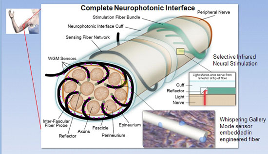
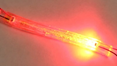
Stretchable Optical Sensor
_______________________________________________________
Fibre Probe Based Raman Spectroscopy Bio-sensor for Surgical Robotics
Application Note
In many surgical procedures involving the excision of tumorous
tissue, the surgeon is challenged in deciding when the excision is
complete whilst at the same time trying to minimise the amount of
healthy tissue removed. This is particularly challenging during
laparoscopy or keyhole surgery, and even more so if robotic surgery is
included, where the view of the tissue and the tactile feedback are
restricted, or absent. Researchers are turning to photonic techniques
such as Raman spectroscopy, which can offer powerful detection
capability in the field of bio-medical optics that aids in the
identification of the chemical constituents of tissues and cells. This
in turn can assist the surgeon in making a reliable diagnosis as regards
the type of tissue. A group at the University of St Andrews [1,2] have
tackled this problem by designing, building and demonstrating a robotic
based analytical tool to assist surgeons in such surgical procedures. Introduction
Many surgical procedures are conducted nowadays with the assistance of robotic systems. Ashok et. al. [1] have developed a Raman probe based system to complement current standard diagnostic techniques such as histological examination. In their design a Raman probe based sensor was integrated into a surgical robot - ARAKNES (Array of Robots Augmenting the KiNematics of Endoluminal Surgery) [3], with the aim of demonstrating a tool for robot-assisted laparoscopic surgery. Laparoscopy is a type of surgical procedure that allows a surgeon to access the inside of the body with keyhole surgery, for example the abdomen, without having to make large incisions in the skin.

Setup
A schematic of the spectroscopy part of the system is shown in figure 1. The Raman sensor consists of four principal subsystems:
- a laser diode operating at 785 nm (LuxxMaster , PD-LD) to excite the sample, with typical input power of 100 mW at the sample,
- a fiber-based Raman probe (Emvision LLC), with an excitation delivery fiber of 200 ?m core diameter, and a collection bundle of 7 fibers each with 200 µm core diameter,
- a spectrometer (Shamrock SR-303i) using an f-number matcher and incorporating a 400 lines/mm grating, blazed at 850 nm to facilitate good collection efficiency,
- a detector (Newton) that has a thermo-electrically (TE) cooled deep-depletion, back-illuminated sensor to ensure optimum sensitivity in the NIR region.

- it could be maneouvred easily by the robotic arm inside the abdominal cavity and,
- the stiffness of the first 30 cm approximately of the fiber probe next to the head could be varied in such a way so as to aid the positioning of the probe head during the insertion and retraction phases of the surgical procedure.
A disposable sterile sleeve, into which the probe was inserted, was used to maintain sterility of the probe during the surgical procedure. A sapphire window was bonded to the end of the sleeve and this allowed optical access to the tissue from the probe head. The probe head was pushed up against the 1 mm thick sapphire window. Since the probe head had a working distance of 1 mm – the sleeve-head assembly was used in contact mode i.e. the sapphire window was brought into contact with the tissue when taking the Raman spectral data, thus minimising any variability in the signal due to different sample-probe distances.
Another very important component of the system was the user-compatible software interface. Clearly the tool has to be user friendly to surgeons and medical staff, whose expertise is not analytical spectroscopy, but who want to know whether the tissue under test is healthy or cancerous. Ashok et. al. implemented a supervised multivariate classification algorithm to classify the different tissue types. Two key features incorporated within their protocol for analysing the data were:
- adapting the configuration to avoid inter-patient variability in data, and,
- ensuring the sensor system is generic for use in binary discrimination between any types of tissue i.e. that it is not restricted to a particular tissue type.
Results and Discussion
In order to test the efficacy of the system, proof-of-principle tests were carried out on excised tissues that were visually similar. Adipose tissues derived from various animals were used in this tissue discrimination analysis. A typical Raman spectrum captured from Bovine adipose tissues is shown in figure 3. With chemometric analysis of the subtle differences between spectral features from different samples the different tissues types can be identified. An accuracy of 95% was obtained in discriminating these tissue types.

________________________________________________________________________________
Robotic Waveguide by Free Space Optics
1. Introduction
Road
construction and work on the water supply often require the relocation
of aerial/underground telecommunication cables. Each optical fiber
leading from an optical line terminal (OLT) in a telephone office to a
customer’s optical network unit (ONU) must be cut and reconnected.
Customers expect real-time transmission for high-quality communications
to continue uninterrupted, especially for video transmission services.
Some
electrical transmission apparatus can maintain communication without
interruption, even when optical cables are temporarily cut. The system
is complicated and any transmission delay during O/E conversion is fatal
to real-time communication. Although it is desirable to directly switch
the transmission medium itself, it had been thought that some data bits
would inevitably be lost during the replacement of optical fibers. An
optical fiber cable transfer splicing system has been developed to minimize the disconnection time. It takes 30 ms to switch a transmission line, and more than 2 seconds * to restore communications with, for example, GE-PON .
We
have developed an interruption-free replacement method for in-service
telecommunication lines, which can be applied to the current PON system
equipped with conventional OLTs and ONUs .
Two essential techniques were presented; a measurement method and a
system for adjusting the transmission line length. The latter
continuously lengthens/shortens the line over very long distances
without losing transmitted data based on free space optics (FSO). The
former distinguishes the difference between the duplicated line lengths
by analyzing signal interference. The mechanism that automatically
coordinates both these two functions and referred to as a robotic
waveguide in this paper compensates for the traveling time difference of
a transmitted pulse. Interferometry is the technique of diagnosing the
properties of two or more lasers or waves by studying the pattern of
interference created by their superposition. It is an important
investigative technique in the fields of astronomy, fiber optics,
optical metrology and so on. Studies on optical interferometry are
reported to improve tiny optical devices . We have applied the technique to measure length of several kilometers of optical fibers with a 10 mm resolution.
This
paper describes the design of our robotic waveguide system. An optical
line length measurement method is studied to distinguish the difference
of two lines by evaluating interfered optical pulses. An optical line
switching procedure is designed, and a line length adjustment system is
prototyped. Finally, we applied the proposed system to a 15 km GE-PON
optical fiber network while adding a 10 m extension to show the
efficiency of this approach when replacing in-service optical cables.
2. Optical line duplication for switching over
Figure 1
shows an individual optical line in a GE-PON transmission system with a
single star configuration. Optical pulse signals at two wavelengths are
bidirectionally transmitted through a regular line between customers’
ONU and an OLT in a telephone office via a wavelength independent
optical coupler, WIC1, and a 2x2 optical splitter, 2x2 SP, respectively.

We
have designed a robotic waveguide system, and a switching procedure for
three wavelengths, namely 1310 and 1490 nm for GE-PON transmission, and
1650 nm for measurement. A robotic waveguide system is installed in a
telephone office. It is composed of an optical line length detector and
an optical line length adjuster. A test light at a wavelength different
from those of the transmission signals is sent from one of the optical
splitter’s ports to the duplicated lines. An oscilloscope is connected
to the optical coupler to detect the test light through a
long-wavelength pass filter (LWPF). The optical line length adjuster is
an FSO application. Some optical switches (SWs) and optical fiber
selectors (FSs) control the flow of the optical signals managed by a
controller. The optical pulses are compensated by 1650 and 1310/1490 nm
amplifiers . The proposed method temporarily provides a duplicate transmission line as shown in Fig. 1
to replace optical fiber cables. A detour line is prepared in advance
through which to divert signals while the existing line is replaced with
a new one. This system transfers signals between the two lines. Signals
are duplicated at the moment of changeover to maintain continuous
communications. The signals travel separately through the two lines to a
receiver. A difference in the line lengths leads to a difference in the
signals’ arrival times. A communication fault occurs if, as a result of
their proximity, the waveforms of the two arriving signals are too
blurred for the signals to be identified as discrete. Thus it is
important to adjust the lengths of both lines precisely. Experiments
determined that the tolerance of the difference in line length is 80 mm
with regard to the GE-PON transmission system.
The
proposed system controls the adjustment procedure so that the
difference in length between the detour and regular lines is adjusted
within 80 mm.
III . Optical line length difference detection
We
use laser pulses at a wavelength of 1650 mm to detect the optical path
length difference. They are introduced from an optical splitter,
duplicated, and transmitted toward the OLT through the active and detour
lines. They are distributed by an optical coupler just in front of the
OLT, and observed with an oscilloscope. The conventional measurement
method evaluates the arrival time interval between the duplicated
signals, and converts it to the difference between the lengths of the
regular line and the detour line at a resolution of 1 m. The difference
in line length, ΔL is described as

where c is the speed of light, Δt is the difference between the signal arrival times for the regular and detour lines, and n is the refractive index of optical fiber.
Figure 2
shows the received pulses observed with an oscilloscope. When the
detour is 99 m shorter than the active line, pulses traveling through
the detour line reach the oscilloscope about 500 ns earlier than through
the regular line. The former pulse approaches the latter as shown in Fig. 2(b),
while the system lengthens the detour line using the optical path
length adjuster. This method fails if the difference between the line
lengths is less than 1 m, because the two pulses combine as shown in Fig. 2(c).
We
also developed an advanced technique for measuring a difference of less
than 1 m between optical line lengths. Interferometry enables us to
obtain more detailed measurements when the optical pulses combine. A
chirped light source generates interference in the waveform of a unified
pulse.
Each pulse, E (Lj, t) is expressed as

where j represents the regular line, 1, or the detour line, 2. And, Aj, k, n, Lj, ωj, t, ϕ0
denote amplitude, wavenumber in a vacuum, refractive index of optical
fiber, line length, frequency, time, and initial phase, respectively.
The intensity of a waveform with interference, I, is calculated by taking the square sum as

where ΔL and Δω represent the differences between line lengths and frequencies, respectively.
The waveform with interference depends on the delay between the pulses’ arrival times. Time-domain waveforms are shown in Fig. 3. When the gap was 0.5 m, the waveform contained high-frequency waves as shown in Fig. 3(a).
The less the gap became, the lower-frequency the interfered waveform
was composed of. When the lengths of two lines coincided, a quite
low-frequency waveform was observed as Fig. 3(d).

Figure 2.
Time-domain optical line length measurement when difference in line length is more than 1 m.

Figure 3.
Time-domain optical line length measurement when difference in line length is less than 1 m.
A
Fourier-transform spectrum reveals the characteristics. When the gap
was 0.5 m, the waveform with interference was composed of the power
spectrum shown in Fig. 4(a). The peak power indicated that the major frequency component was around 600 MHz. Figure 4(b) and (c)
indicate that the peak powers for gaps of 0.3 and 0.1 m were 360 and
120 MHz, respectively. It became difficult to determine the peak for
smaller gaps, because the frequency peak became so low that it was
hidden by the near direct-current part of the frequency component. When
the lengths of duplicated lines coincided, the power spectrum was
obtained as Fig. 4(d).

An
evaluation of the frequency characteristics in the interfered waveforms
showed that the peak frequencies are proportional to the difference
between the line lengths from -1 to 1 m as shown in Fig. 5.
This result helps us to determine the optimal position for adjustment.
The optimal position where the line lengths coincide can be estimated by
extrapolating the data.
We have established a
technique for distinguishing the difference between line lengths to an
accuracy of better than 10 mm by analyzing interfering waveforms created
by chirped laser pulses.
We have realized a complete length measurement for optical transmission lines from 100 m to 10 mm.

IIII . Robotic waveguide system
We
designed a prototype of the robotic waveguide system to apply to a
GE-PON optical fiber line replacement according to the procedure
described below.
An optical line length adjuster, shown in Photo 1,
is installed along the detour line. The adjuster is equipped with two
retroreflectors, which directly face each other as shown in Fig. 6.
A retroreflector consists of three plane mirrors, each of which is
placed at right angles to the other two. And it accurately reflects an
incident beam in the opposite direction regardless of its original
direction, but with an offset distance. The vertex of the three mirrors
in the retroreflector is in the middle of a common perpendicular of the
axes of the incoming and outgoing beams as shown in Fig. 6.
The number of reflections is determined based on the retroreflector
arrangement. A laser beam travels 10 times between the retroreflectors
in our prototype, and are introduced into the other optical fiber.
Optical pulses are transmitted through an optical fiber, divided into
three wavelengths by wavelength division multiplexing (WDM) couplers,
and discharged separately into the air from collimators. The focuses of a
pair of collimators corresponding for a wavelength is best tuned for
the wavelength to achieve the minimum coupling loss. The collimators for
multiple wavelenghts are arranged to share the two retroreflectors as
shown in Fig. 7.
The detour line between the retroreflectors consists of an FSO system .
The detour line length can be easily adjusted by controlling the
retroreflector interval with a resolution of 0.14 mm. Optical pulses
travel n-times faster in the air than in an optical fiber, where n is
the refractive index of the optical fiber. Thus the optical line length
adjuster lengthens/shortens the corresponding optical fiber length, L, by kΔx/n, where k, Δx, n
are the number of journeys between the retroreflectors, the
retroreflector interval variation, and the refractive index of optical
fiber, respectively. The FSO lengthens the optical line length up to L0.


where Δxmax is the maximum range of the retroreflector interval variation. The maximum range of our prototype, Δxmax, is around 0.3 m, the refractive index, n, of the optical fiber is 1.46, the number of journeys, k is 10, and the optical line span, L0, tuned by the adjuster is 2 m.


The
limit of the adjustable range is a practical problem when this system
is applied to several kilometers of access network. Therefore, we employ
optical line length accumulators. The optical line length adjuster
contains two optical paths, #0 and #1 as shown in Fig. 1 or Fig. 8.
An optical switch and an optical fiber selector are installed in each
path. Optical switches control the optical pulse flow. Each optical
fiber selector is equipped with various lengths of optical fiber, for
example L0, 2L0 and 3L0. The path length can be discretely changed by choosing any one of them.
The optical line length adjuster can extend the detour line as much as required using the following operation as shown in Fig. 9. First, the FSO system lengthens path #0 by L0 by gradually increasing the retroreflector interval. After the optical fiber selector has selected an optical fiber of length L0,
the active line is switched from path #0 to path #1. The FSO system
then returns to the origin, and the optical fiber selector selects an
optical fiber of length L0 instead to keep the length of path #0 at L0.
The FSO system increases the retroreflector interval again to repeat
the same operation. In this way the adjuster accumulates spans extended
by the FSO system. The scanning time of our prototype is 10 seconds,
because the retroreflector operates at 30 mm/s.
The optical line length adjuster enables us to lengthen/shorten the detour line while continuing to transmit optical signals.

IIIII . Experiments on optical line replacement
The optical line replacement procedure, shown in Fig. 10 where a 2x8 optical splitter is used instead of a 2x2 splitter, is as follows:
- A detour line is established between a WIC and a 2x8 optical splitter.
- The detour line length is measured with a 1650 nm test light using an optical line length measuring technique, and is adjusted to the same length as the regular line using an optical line length adjusting technique. These techniques are described in the preceding sections.
- Once the lengths of the two lines coincide, the transmission signals are also launched into the detour line.
- The regular line is cut and replaced with a new line, while the signals are being transmitted through the detour line. A long-wavelength pass filter (LWPF) is temporarily installed in the new line.
- The test light measures the lengths of the new line and the detour line. The detour line is adjusted to the new line while communications are maintained. The LWPF prevents only the optical transmission pulses from traveling through the new line.
- The LWPF is then removed and the transmission is duplicated. The detour line is finally cut off.

We
investigated the tolerance of the multiplexed signal synchronicity in
advance. The transmission quality is observed by changing the difference
between the duplicated line lengths. The results show that the
transmission linkage is maintained if the difference is within 80 mm as
with GE-PON. A multiplexed signal cannot be perceived as a single bit
when the duplicated line lengths have a larger gap for 1 Gbit/s
transmission. Because these characteristics depend on the periodic
length of a transmission bit, the requirement is assumed to be severe
when the method is applied to higher-speed communication services.
Next, we constructed a prototype of the robotic waveguide system shown in Fig. 1,
and applied it to a 15 km GE-PON optical transmission line replacement.
A 10 m optical fiber extension was added to the transmission line,
while optical signals were switched between the duplicated lines during
transmission.
Figure 11
shows the frame loss that occurred during optical line replacement,
which we measured with a SmartBit network performance analyzer. No frame
loss was observed at any switching stage if the difference between the
duplicated line lengths was less than 80 mm. If the difference exceeded
80 mm, signal multiplexing caused frame loss in stages (a) and (d). We
confirmed that the optical signals can be completely switched between
the regular, detour, and new lines on condition that the line length is
adjusted with sufficient accuracy.
The
experimental results proved that our proposed system successfully
relocated an in-service broadband network without any service
interruption.

Figure 11.
Frame
loss while replacing transmission line according to the procedure; (a)
Multiplex signals of current line and detour line, (b) Cut current line,
(c) Extend detour line, (d) Multiplex signals of detour line and new
line, (e) Cut off detour line.
IIIIII . Conclusion
We
proposed a new switching method for in-service optical transmission
lines that transfers live optical signals. The method exchanges optical
fibers instead of using electric apparatus to control transmission
speed. The robotic waveguide system is designed to apply to duplicated
optical lines. An optical line length adjuster, designed based on an FSO
system, continuously lengthened the optical line up to 100 m with a
resolution of 0.1 mm. An optical line length measurement technique
successfully evaluated the difference in length between the duplicated
lines from 100 m to 10 mm. An interferometry measurement distinguished
the difference between line lengths to an accuracy of better than 10 mm
by analyzing interfering waveforms created by chirped laser pulses. We
applied this system to a 15 km GE-PON network and succeeded in replacing
the communication lines without inducing any frame loss.
________________________________________
The BigBOSS Instrument
5.1 Overview
The BigBOSS instrument is composed of a set of telescope prime focus corrector optics, a massively multiplexed, roboticized optical fiber focal plane, and a suite of fiber-fed medium resolution spectrographs, all coordinated by a real-time control and data acquisition system. The conceptual design achieves a wide-field, broad-band mulit-object spectrograph on the Mayall 4-m telescope at KPNO.Table 5.1 summarizes the key instrument parameters such as field of view, number of fibers, fiber size and positioning accuracy, spectrograph partitioning, and integration time, were derived from a blend of science requirements and technical boundaries. These were derived from a confronting the science requirements for the Key Science Project with realistic technical boundaries.

Figure 5.1: BigBOSS instrument installed at the Mayall 4-m telescope. A new corrector lens assembly and robotic positioner fiber optic focal plane are at mounted at the prime focus. The yellow trace is a fiber routing path from the focal plane to the spectrograph room incorporating fiber spooling locations to accommodate the inclination and declinaton motions of the telescope. The two stack-of-five spectrograph arrays are adjacent to the telescope base at the end of the fiber runs.
The instrument wavelength span requirement of 340–1060 nm was determined by the need to use galaxy [O II] doublet(3727Å and 3729Å) emission lines to measure the redshift of Luminous Red Galaxies (0.2 < z < 1) and Emission Line Galaxies (0.7 < z < 1.7) and the Ly-α (1215Å ) forest for Quasi-Stellar Objects(2 < z < 3.5) as described in Section 2.
Our large, 3° linear FOV was set by a requirement to accomplish a 14,000 deg2 survey area in 500 nights at the required object sensitivity. The field was selected following feasible designs that were demonstrated in earlier NOAO work and expanded upon with BigBOSS studies. In our implementation, the existing Mayall prime focus is replaced with a six element corrector illuminating the focal plane with a f/4.5 telecentric beam that is well matched to the optical fibers acceptance angle. In this way, the large FOV can be accomplished within a total optical blur budget of 28 µm RMS.
Given the FOV and required number of objects to observe, we design the focal plane to accommodate 5000 fibers by using demonstrated 12 mm pitch fiber actuators. A 120 µm fiber core size is chosen to fit a 105 µm FWHM image of a galaxy (after telescope blur and site seeing of 1 arcsec RMS) while minimizing inclusion of extraneous sky background. The fiber size choice allows for fiber tip placement of 5 µm RMS accuracy.
In order to achieve spectral resolutions of 3000–4000 for resolving the [O II] doublet lines while keeping the optical element small and optimized for high throughput, we have chosen to divide the system into ten identical spectrographs each with three bandpass-optimized arms. with each spectrograph recording 500 fibers and each arm instrumented with 4k×4k CCD.
The exposure time of 16.6 minutes is based on the requirement that at least one of the lines of the [OII] doublet lines 3727Å and 3729Å from an Emission Line Galaxy with a line flux of 0.9×10⁻¹⁶ ergs/cm2/s is detected with a signal-to-noise ratio of 8. The time was derived using the BigBOSS exposure time calculator described in Appendix A and including known detector characteristics (readnoise, dark current, and quantum efficiency), effective telescope aperture, mirror refection, fiber coupling and transmission losses, and spectrograph throughput, A one minute deadtime between exposures was set to maintain the needed observing efficiency while allowing for spectrograph detector reads, fiber positioning, and telescope pointing.
Figures 5.2 and 5.3 schematically show the content and interplay of instrumental systems.

Figure 5.2: BigBOSS telescope system block diagram.

Figure 5.3: BigBOSS focal plane and spectrograph systems block diagram.
5.2 Telescope Optics
5.2.1 Design
BigBOSS employs a prime focus corrector to provide a telecentric, seeing-limited field to an array of automated fiber positioners. Basic design requirements are listed in Table 5.2. The optics team received considerable guidance and assistance from Ming Liang in the areas of corrector, atmospheric dispersion compensator, and stray light design. The final corrector and ADC design was developed from a concept presented by on the NOAO web site ([Liang, 2009]).
Cassegrain and prime focus options were explored. Prime focus was selected for its superior stray light performance, increased throughput due to simplified baffling and smaller central obscuration, and lower cost. The corrector includes four corrector elements, and a pair of ADC elements (each consisting of two powered prisms). Materials and design of the corrector and ADC were selected for manufacturing feasibility. All elements of the corrector are long-lead items, and initial contacts have been made with raw material suppliers and lens manufacturers. Corning can supply the large fused silica pieces, and N-BK7 and LLF1 are current production glasses at Schott.
Figure 5.4 shows the optical layout of the BigBOSS prime focus corrector and ADC. The four singlet corrector elements are fused silica, each with one aspheric and one spherical surface. Element C1 is the largest lens, 1.25 m fused silica. Lens elements were sized to have more 15 mm of radius beyond the clear aperture to allow for polishing fixturing and mounting. The ADC consists of two wedged doublets, with spherical external surfaces, and a flat, cemented wedge interface. ADC elements are made of LLF1 and N-BK7, and all are within the current production capability of Schott. A minimum 300 mm gap exists between Element 4 and the central fiber positioner (focal surface).

Figure 5.4: BigBOSS prime focus corrector consists of four corrector elements and two ADC prism doublets.
Figure 5.5 shows the ideal rms geometric blur performance (no manufacturing, alignment or seeing errors) of the BigBOSS corrector mounted on the Mayall telescope. For reference, the required FWHM geometric blur of 0.8 arcsec corresponds to a blur RMS of 28 µm, so realistic manufacturing margins exist.
Figure 5.5: Ideal geometric blur performance of BigBOSS corrector on Mayall 4-m telescope. The required 0.8 as FWHM corresponds to a geometric blur radius of 28 µm.
5.2.2 Focal Surface
The focal surface is a convex sphere of 4000 mm radius of curvature and has a diameter of 950 mm. This is the surface that the optical fiber tips must placed on to 10 µm accuracy.5.2.3 Tolerancing
The Mayall telescope is seeing-limited with an atmospheric FWHM of 0.9 arcsec, or 72 µm FWHM. For the 17.1 m focal length of BigBOSS, this corresponds to an RMS radius of 32 µm. Peak geometric blur (multispectral) of the perfect telescope across the 3° FOV is 18.3 µm, or 43 µm FWHM. With manufacturing, alignment and thermal drift, the telescope geometric blur is 28 µm RMS, or 66 µm FWHM. The overall peak budget for seeing, residual phase error, manufacturing, alignment error and thermal drift is 100 µm FWHM, or 1.2 arcsec. This is a worst-case number, and performance of the telescope is better over the majority of the field.Tolerances for the telescope are broken down into three major categories: compensated manufacturing errors, compensated misalignment, and uncompensated errors. Manufacturing errors such as lens radius of curvature and thickness may be compensated to a certain degree by varying the spacing of the lens elements during assembly and alignment. Table 5.3 shows compensated manufacturing tolerances on the individual optical elements.
 Residual alignment errors and thermal drift in the assembled corrector
are compensated by a motion of the entire corrector barrel and focal
plane via motorized hexapod. Residual errors after these compensations
are primarily higher-order aberrations, and are budgeted
as compensated tolerances in Table 5.4.
Residual alignment errors and thermal drift in the assembled corrector
are compensated by a motion of the entire corrector barrel and focal
plane via motorized hexapod. Residual errors after these compensations
are primarily higher-order aberrations, and are budgeted
as compensated tolerances in Table 5.4.
The current operations plan involves characterization of the telescope for gravity sag as a function of elevation, and thermal drift of telescope focus. These are compensated continuously by motion of the hexapod. Other manufacturing errors may not be compensated (between observations) by motion of the hexapod, for example, corrector glass inhomogeneities. Such effects are currently being quantified, but the optical performance of the corrector (geometric blur) has more allowance than other existing and planned (e.g., DES) designs.

5.2.4 Optical Mounts
Corrector and ADC elements have coefficients of thermal expansion between 0.5 and 8.1 ppm/°C. The largest element is corrector element C1 (1.25 m in diameter). Operational temperatures range from -10° to 30° . Although larger transmissive elements have been built, detailed design and careful attention will be necessary during the design, fabrication and test phases in order to achieve the science goals of BigBOSS.Overall responsibility for mounting and aligning the large glass elements of the corrector lies with University College London (UCL), who is also responsible for the similar corrector barrel assembly for DES. Requirements and goals for the optical mounts are listed in Table 5.5.
 The glass elements of the corrector will be mounted in rigid lens cells
with a compliant layer interface. A nickel/iron alloy will be used as
the cell material with RTV rubber pads as the interface between cell and
lens. With a suitable choice of the Ni/Fe alloy mix, a particular CTE
can be chosen which in combination with precise thickness RTV pads
around the perimeter of the silica lens allow an athermal design that
allows the lens to expand and contract with minimal stress. Once mounted
in the cell, standard fastener construction can be used to mount the
lens cell via a metal ring to the barrel.Titanium cell rings (9.2×10⁻⁶/°C) are used with RTV to similarly athermalize the higher expansion N-BK7 and LLF1 lenses (6.2×10⁻⁶/°C and 7.1×10⁻⁶/°C
respectively). A circular array of flexure blades allows for thermal
expansion between the lens cell and the corrector barrel. This heritage
design is currently being implemented by UCL on the DES project (see
Figure 5.6b).
The glass elements of the corrector will be mounted in rigid lens cells
with a compliant layer interface. A nickel/iron alloy will be used as
the cell material with RTV rubber pads as the interface between cell and
lens. With a suitable choice of the Ni/Fe alloy mix, a particular CTE
can be chosen which in combination with precise thickness RTV pads
around the perimeter of the silica lens allow an athermal design that
allows the lens to expand and contract with minimal stress. Once mounted
in the cell, standard fastener construction can be used to mount the
lens cell via a metal ring to the barrel.Titanium cell rings (9.2×10⁻⁶/°C) are used with RTV to similarly athermalize the higher expansion N-BK7 and LLF1 lenses (6.2×10⁻⁶/°C and 7.1×10⁻⁶/°C
respectively). A circular array of flexure blades allows for thermal
expansion between the lens cell and the corrector barrel. This heritage
design is currently being implemented by UCL on the DES project (see
Figure 5.6b). 
Figure 5.6: Schematic of athermalized, flexure-mounted lens cell design (left) and 550 mm prototype lens and lens cell at UCL (right).
5.2.5 Coatings
The preferred coating technology for the BigBOSS lenses is a hard (and durable) coating of MgF2, with a tuned Sol-Gel coating. While Sol-Gel can be tuned to some degree for the bandpass of the telescope, it is not as durable as MgF2. Cost, risk, performance and alignment constraints on the various coating technologies will be investigated during the fabrication of the corrector lenses, and a final decision is not necessary at this time. The likely configuration for the coatings is a hybrid MgF2 undercoat with a tuned Sol-Gel overcoat (demonstrated performance of <0.5% loss over the visible band). At least two vendors (REOSC and SESO) are capable of coating the optics, including the 1.25 m diameter C1 element. It is expected that improved capability will be available subsequent to lens polishing.5.2.6 Stray Light and Ghosting
A major benefit, and reason for selecting the prime focus option over Cassegrain, is the simplified stray light baffling. A wide-field Cassegrain design appropriate for BigBOSS would require a 50% linear obscuration, with carefully designed M1 and M2 baffles in order to block direct sneak paths to the detector. With a prime focus design, out-of-field rays miss the focal plane entirely. The main sources of stray light (first order stray light paths) are surfaces illuminated by sky light, and directly visible to the focal plane. Chief among these surfaces are the structure surrounding M1, which will be painted with durable diffuse and specular black stray light coatings (Aeroglaze Z302, Z306 and Ebanol). Other first order stray light paths include particulate contamination on M1 and the surfaces of the correctors.The BigBOSS corrector was designed to ensure internal reflections within the corrector do not contribute significantly to stray light at the focal surface. The main causes of reflections are typically reflections off concave surfaces (facing the focal surface), and are most significant for elements in close proximity to the focal surface. Figure 5.7 shows a ghost stray light path from the C4 corrector element, which has been reduced by ensuring the radius of curvature of the first optical surface is smaller than its separation from the focal plane. As shown, the focus of the ghost is located off the focal surface, and only a diffuse reflected return, off two surfaces with >0.98% transmission surfaces contributes to the stray light at the focal plane. Additional point source transmittance analysis with realistic contamination and surface roughness is currently underway with the existing stray light model of the telescope and corrector.
Reflections between the focal plane array and nearby corrector surfaces are a typical source of stray light in an imaging wide-field corrector system. Because the fiber positioners can be made rough, and painted black, this source of stray light may be virtually eliminated on a robotic fiber array.

Figure 5.7: Reflections off corrector lens surfaces could contribute ghost background noise. Elements are designed to reduce bright ghost irradiance on the focal plane to acceptable levels.
5.2.7 Atmospheric Dispersion Corrector
Chromatic aberration must be sufficiently small to place incoming light between 0.34–1.060 nm within the geometric blur allocation. Because observations will be between 0−60° from zenith, an atmospheric dispersion corrector will be necessary. The ADC elements are 0.9 m in diameter and made of Schott LLF1 and N-BK7. Wedge angles within the two elements are roughly 0.3° . Figure 5.8a shows the PSF across a 3 ° FOV at an angle 60° from zenith with the ADC rotated to correct for atmospheric dispersion. Figure 5.8b is for the uncorrected case. Rotational tolerance requirements for the ADC are greater than 1°, and the ADC rotator is consequently not a high-precision mechanism.5.2.8 Hexapod Adjustment Mechanism
Compensations for gravity sag, temperature change and composites dryout will be provided by a six-degree-of-freedom hexapod mechanism, Figure 5.9. The focal plane and corrector elements are positioned relative to one-another during alignment, and moved as a unit by the hexapod. Requirements for the hexapod are as listed in Table 5.6.
Figure 5.8: Geometric raytrace shows effects of atmospheric dispersion on telescope point spread function. a) A heavily chromatically aberrated view of the sky 60° from zenith. Overall scale is 1m square, PSF exaggerated by factor of 106. This chromatic aberration is removed by rotating the ADC prisms 85° as shown in b). The dispersion being compensated here is 3 arcsec.

5.2.9 Telescope Simulator
The corrector integration and testing will be performed at FNAL using a telescope simulator developed for the DECam Project at the Blanco telescope, the twin of the Mayall. The telescope simulator (see Figure 5.10) will allow us to prove that the corrector passes the technical specifications independent of the expected orientations of the telescope. This platform will also allow us to develop the procedures that will be used to install the focal plane on the telescope. Performing this work in the lab, rather than in the field, we reduce the risk of extended telescope down-time when we install the instrument on the telescope for the first time, and we minimize the amount time required for integration and commissioning at KPNO.The telescope simulator base is 4.3 m tall and 7.6 m wide. The four rings weigh 14,500 kg. The outer one has a 7.3 m diameter. Two motors from SEW Eurodrive can orient the camera to any angle within the pitch and roll degrees of freedom. The pitch motor is 1/3 HP, 1800 RPM, directly-coupled, torque-limited and geared down 35,009:1 for a maximum speed of 20 minutes per revolution. The roll motor is 1/2 HP, 1800 RPM, geared down 709:1 for a maximum speed of 11.5 minutes per revolution. The coupling is by means of a 18.9 m chain attached to the inner race (3rd ring out). Of course, the motor controls allow the assembly to be moved more slowly. When the assembly is not moving, the motors automatically engage brakes. The motors are controlled from a panel located on the exterior of the base. These controls are simple power on/off, with forward/backward and speed control for each ring. Four limit switches prevent the rings from being oriented in any undesired location.

Figure 5.9: The corrector is supported on a six-degree-of-freedom hexapod mechanism that attached to the telescope structure through a series of rings and struts. Four of the hexapod actuators are the cylinders in the center of the figure (red). The cylinders at the left (blue) form the passive kinematic mount of the focal plane to the corrector.
5.2.10 Fiber View Camera
During the course of the survey, before any given exposure, after the mechanism to arrange the position of the 5000 fibers has completed its task the Fiber View Camera will take a picture of the fibers on the fiber plane to check the accuracy of all of the fiber positions, and if needed allow the correction of any misplaced fibers. The camera will be located on the axis of the telescope at a distance of 1 m below corrector element C1, as shown on Figure 5.11. The camera will be supported in this position by thin spider legs from the ring supporting the first element of the corrector optics. In this position the lens of the fiber view camera will be 5 m from the fiber plane. To get an image of the 950 mm diameter fiber plane on a 40 mm CCD will require the camera to have a demagnification of about 25. This can be accomplished with a 200 mm focal length lens. A detailed ray tracing through the camera lens and corrector optics finds that the image sizes are too small so we will have to defocus the camera to get the images to spread out over enough pixels to allow good interpolation. The fibers will be back-illuminated at the spectrograph end by a 10 mW LED.
Figure 5.10: The telescope simulator at Fermilab with the DECam Prime Focus Cage. The structure in the background supports a copy of the two rings (white) at the top of the Serrurier Truss. The yellow rings are connected to motor drives that enable the Prime Focus Cage to be pitched and rolled, for the purpose of testing and pre-commissioning of the instrument prior to delivery to the telescope. The foreground structure (left) is the secondary (f/8) mirror handling fixture, enabling the installation of the mirror over the end of the optical corrector for the use of instruments at the Cassegrain Focus.
The view camera images the fiber tip focal plane through the corrector optics. This introduces some distortions in the images. A detailed study of the image shapes, using the BEAM4 ray tracing program, shows that these distortions are at an acceptable level. A set of fixed and surveyed reference fibers will be mounted in the focal plane and imaged simultaneously with the movable fibers. These can be used to deconvolve any distortion and any motion of the camera with respect to the focal plane due to gravity sag.5.2.10.1 Design Considerations. The performance requirements for the fiber view camera are summarized in Table 5.7. We note further that since we plan to illuminate the fibers with a monochromatic LED, the CCD of choice should be monochromatic. For this reason we will use a monochromatic CCD, the Kodak KAF-50100. The plan is then to build a custom camera body (see Figure 5.12) using a commercially available lens, the Canon EF 200 mm f/2.8 L II USM. There also exists commercially available clocking and readout electronics for the Kodak CCD that we plan to use.
5.2.10.2 Fiber Illumination. We plan to illuminate each fiber at their end in the spectrometer with a monochromatic 10 mW LED. We estimate that each fiber will emit 2×10⁹ photons/sec into a 30° cone, full angle, at the focal surface. The solid angle of the fiber view camera lens will capture 3×10⁵ photons/sec/fiber image. With 25% quantum efficiency this gives 75,000 electrons/sec/fiber image on the CCD.
5.2.10.3 Dark Current and Read Noise. It is desirable to run the camera at room temperature. The dark current in this Kodak CCD is advertised as 15 e/pixel/sec at 25°C and the read noise is 12.5 e at a 10 MHz read out rate. Both of these are quite negligible compared to the high fluxes expected from the fibers.

Figure 5.11: The Mayall Telescope showing the placement of the corrector optics and the fiber view camera

Figure 5.12: Schematic of the Fiber View Camera
5.2.10.4 Fiber Position Precision. With a demagnification of 25 the 120 µm diameter fiber will have a 5 µm diameter image on the CCD. Including the optical distortions we still expect image sizes well under 10 µm, not a match to the 6 µm CCD pixels. We plan to defocus the lens slightly to produce large enough images to allow interpolations to much better than the pixel size. A Monte Carlo calculation was performed to determine the optimal image size. For the discussion here we will assume a 25 µm diameter image with significant flux spread over 16 pixels. With a one second exposure we expect 75,000 electrons per image. With such large signal to noise, we expect to centroid the fiber position to ~0.1 µm. Systematic effects can double this to 0.2 µm. With the factor of 25 demagnification this translates to a 5 µm measurement error on the fiber plane.5.2.10.5 Occupancy and Ability to Resolve Close by Fibers. With 16 pixels in a fiber image, the 5000 fibers will occupy 80,000 pixels. Compared to the 50×106 pixels on the CCD, this gives an acceptable occupancy of ~2×10⁻³ . The fiber positioning mechanism sets the closest separation between any two fibers to be 3 mm. With the factor of 25 demagnification this means 120 µm or a 20 pixel separation on the CCD, so that overlap of the images will not be a problem. We have developed code to carry out a simultaneous fit to two images when two images are close together so that the tails of one image under the other and vice versa are correctly taken into account.
5.2.10.6 Modelling and Scene Calibration. The fiber position measurement preci sion quoted in Table 5.7 is based on the assumption that given the high statistics we can measure the position of the centroid of the image on the CCD to 3% of the pixel size. A Monte Carlo simulation will be useful to determine the optimum image size on the CCD for the best precision. In addition to the statistical error there will be systematic effects that limit the precision, such as variations in pixel size and response, lens distortions, etc. Before installation of the camera on the telescope a measurement and calibration of the precision in a test set up is anticipated.

5.3 The Focal Plane Assembly
The BigBOSS focal plane assembly includes three main items: the support structure (adapter), the focal plate (which supports the ~5000 actuators) and the set of actuators. The focal plane system is being studied by the Instituto de Astrof´ısica de Andaluc´ıa (IAA-CSIC, Granada, Spain). The IAA-CSIC, in collaboration with the company AVS, is working on its conceptual design. The focal plane parameters depend heavily on the support structure (corrector barrel) and on the final design of the fiber positioners (actuators). The focal surface is as a convex spherical cap with 4000 mm radius of curvature and 950 mm in diameter. The focal plate is foreseen to be an aluminum alloy plate ~100 mm thick. Its primary purpose is to support the fiber positioners such that the fibers patrol area form tangents to the focal surface. The focal plate will be attached to the corrector barrel through a support structure, that we call “adapter”. Figure 5.13 shows a view of the whole system.5.3.1 Interfaces
The focal plate must be held at the back of the corrector barrel, facing the last lens of the corrector. Due to the distance to the corrector (about 200 mm), the focal plate cannot be directly attached to the corrector barrel and some structure in between (adapter) will be necessary. This will need to provide manual adjustment for initial focusing.
Figure 5.13: A cross section of the focal plane assembly with a possible shape of the focal plate and the adapter to attach the focal plate to the corrector barrel (orange color). The detail of a single actuator supporting a fiber is shown enlarged.
The focal plane supports several systems, most importantly being the 5000 fiber positioners. These will be inserted from the back of the focal plane to facilitate replacement. Insertion depth, tilt and rotation angle are precisely controlled, tolerances allocated from an overall focus depth budget. An array of back illuminated fixed fibers will serve as fiducials for the fiber view camera. Guiding and focus sensors also reside on the focal plane.The focal plane is electrically connected to the power supplies for the fibers positioners, positioners wireless control system, electronics for guiding and focusing sensors, fiber view camera lamps, and environment monitors. Electromagnetic interference, both received and transmitted, will need careful study.
The large number of fibers and cables coming from the prime focus necessitate careful placement. They will be routed from the focal plane to the telescope support cage while minimizing obscuration of the primary mirror. Careful packing within the footprint of the primary optics support vanes coming from the telescope Serrurier truss will be designed.
5.3.2 Focal Plate Adapter
A structure is needed in order to attach the focal plate to the corrector barrel. A simple structure made of two circular flanges linked by a number of trusses should be able to cope with the flexures and sag. A few reference pins will be used to obtain mounting repeatability.Interface of the adapter will be the corrector barrel on one side, and the focal plate edge on the other side. The adapter requirements are shown in Table 5.8.

5.3.3 Focal Plate
The focal plate will be a solid piece of metal, probably an aluminum alloy, with multiple drills for actuator housing. The plate does not need to have a spherical shape, but the holes hosting the actuators must have their axes converging to the focal surface center and the plate must support the actuators so that their tips lie on the spherical focal surface. An example of suitable shape is shown in Figure 5.13. The edge of the plate must match the adapter flange that attaches to the corrector barrel. A few reference pins will be used to obtain a repeatable positioning onto the flange. Because the holes hosting the actuators do not follow any regular pattern (see Fiber Positioner Topology section), they will have to be machined from the model coordinates via a 5-axes machine tool. Care must be taken with the thermal expansion of such a large metal plate (aluminum alloys might not be ideal in this respect), which could easily overcome the actuators required positioning precision. A detailed materials study will be conducted in order to constrain the thermal effects as much as possible. Eventually, it could be necessary to set up a thermally controlled environment around the plate and the actuators, which could be obtained by enclosing the back of the focal plane with a vacuumed box, the other side of the focal plane being enclosed by the corrector last lens. Analysis is ongoing for studying the behavior of the honeycomb focal plate structure in terms of stiffness, deformations, sag etc. Such parameters vary with the inter-actuator wall thickness and plate thickness, but also depend on the actuator characteristics (once mounted, the actuators will contribute importantly to the stiffness and weight of the focal plane). In general, during the focal plane integration and test, it will be necessary to characterize all the reference positions of the actuators via the fiber view camera (with fiber back-illumination), which makes it much easier to fulfill the positioning precision requirement over such a large array of actuators. The requirements for the focal plate are shown in Table 5.9.
5.3.4 Fiber Positioners
A key enabling element for an efficient survey is a robotically manipulated fiber positioning array. The ability to reposition the fiber array on a timescale of ~1 min greatly improves on-sky operational efficiency when compared to manual fiber placement methods. Require ments for the fiber positioner system are shown in Table 5.10. The fiber positioners selected for BigBOSS will be assembled by the China
USTC group, who has experience designing and manufacturing the
actuators for the LAMOST project. Several variants of the LAMOST
actuators, specifically designed for BigBOSS, are currently under test at
USTC. Current BigBOSS designs include a 10 mm diameter (12 mm pitch)
actuator, as well as a 12 mm and 15 mm diameter variant. The 12 mm
diameter version
(see Figure 5.14) has a measured positioning repeatability (precision) of better than 5
µm. Key changes to the LAMOST design include installation of
smaller diameter motors with co-linear axes, and a redesign of the gear
system. The LBNL/USTC team is currently working to achieve a 10 mm
diameter (12 mm pitch) actuator. The Instituto de Astrofísica de
Andalucía (IAA-CSIC, Granada, Spain) in collaboration with the company
AVS is in parallel working on a separate design for a BigBOSS 10 mm
diameter actuator. The two designs will be reviewed and, finally, the
best of each will be used for the BigBOSS actuator. IAA-CSIC/AVS has
extensive experience with the design, construction and testing of a high
precision fiber positioner prototype for the 10 m Gran Telescopio
Canarias.
The fiber positioners selected for BigBOSS will be assembled by the China
USTC group, who has experience designing and manufacturing the
actuators for the LAMOST project. Several variants of the LAMOST
actuators, specifically designed for BigBOSS, are currently under test at
USTC. Current BigBOSS designs include a 10 mm diameter (12 mm pitch)
actuator, as well as a 12 mm and 15 mm diameter variant. The 12 mm
diameter version
(see Figure 5.14) has a measured positioning repeatability (precision) of better than 5
µm. Key changes to the LAMOST design include installation of
smaller diameter motors with co-linear axes, and a redesign of the gear
system. The LBNL/USTC team is currently working to achieve a 10 mm
diameter (12 mm pitch) actuator. The Instituto de Astrofísica de
Andalucía (IAA-CSIC, Granada, Spain) in collaboration with the company
AVS is in parallel working on a separate design for a BigBOSS 10 mm
diameter actuator. The two designs will be reviewed and, finally, the
best of each will be used for the BigBOSS actuator. IAA-CSIC/AVS has
extensive experience with the design, construction and testing of a high
precision fiber positioner prototype for the 10 m Gran Telescopio
Canarias. The choice of power and command signaling architecture for the robotic actuators is driven by packaging constraints. LAMOST experience shows that fiber, power and command line routing space is at a premium on a high-density robotic focal plane array. LAMOST opted to implement a hybrid wire/wireless scheme, in which only power lines and fibers were connected to each actuator and commanding was implemented by a ZigBee® 2.4 GHz wireless link. Based on this experience, BigBOSS has baselined ZigBee wireless communication. We have discussed with UC Berkeley and LBNL people working with the ZigBee standards committee and they indicated that this is good application and will be more so with an upcoming revision to the standard. Five transmitters will communicate with 1,000 actuators. The thermal cover on the aft end of the corrector will serve as a faraday cage to contain RF transmission from the ZigBee array. Although ZigBee commanding is currently baselined, power-line commanding is also under consideration.

Figure 5.14: 12 mm diameter actuator under test at USTC
Figure 5.15 shows the baseline actuator control board as implemented by USTC, and the overall architecture. In order to reduce the size of the board compared to that of LAMOST, a smaller microcontroller (without integral ZigBee) was selected. The power converter of the LAMOST board was made unnecessary by selecting a motor driver, microcontroller and ZigBee IC that operate at the same voltage. Each group of 250 actuators will be powered by one dedicated 250 W power supply.
Figure 5.15: BigBOSS wireless actuator control board is 7 mm wide, with 4-layers. This USTC design is simplified compared to that of LAMOST.
5.3.5 Fiber Positioners Placement
Each fiber tip must be positionable within a disc (patrol disc) in order to gather the light of a targeted galaxy. In order to cover all the focal plane, the patrol discs must overlap as shown in Figure 5.17, top-left panel. This is possible thanks to the fiber being mounted on an arm which can protrude from the actuator chassis envelope. The positioning software must be clever enough so as to avoid collisions between arms of different actuators (simulations performed at IAA-CSIC show that this is possible). The patrol disc is necessarily flat because of the positioner characteristics, but the fiber tips should lie on a convex spherical focal surface, with a radius of curvature of 4000 mm and a diameter of 950 mm. Two questions arise:5.3.5.1 What is the best position of the disc with respect to the spherical focal surface? Placing the disc tangent to the sphere is not ideal because the borders of the disc would be affected by defocusing. The same is true if the circumference of the disc is embedded in the spherical surface; in this case the center of the disc would suffer the defocusing. The best position must be somewhere between these two extreme positions, and we assume it to be that position for which the defocus is the same at the center and at the border of the patrol disc (other positions could be used, with little practical difference). Figure 5.16) illustrates the trades. For a 4000 mm radius of curvature, and 6.93 mm patrol radius, and imposing W = S (see Figure 5.16), the amount of defocus is identical at the center and at the border of the patrol disc. The best position is found with the patrol disc 2.5 µm away from being tangent to the focal surface. It also tells us that the defocus at the center and border of the patrol disc is also 2.5 µm.

Figure 5.16: Cross section of a patrol disc (the vertical line) when intersecting the focal surface (curved line). S and W are the deviations in and out of the focal plane.
5.3.5.2 Is it possible to distribute the actuators uniformly over the spherical surface? Here, “uniformly” means that the distances between the centers of one patrol disc and its six neighbors (a hexagonal pattern is assumed) is the same over the whole focal plane. A sphere can not be tessellated with uniform size hexagons, thus a compromise must be accepted and the final pitch between actuators will necessarily vary across the focal plane. The task is then to find a distribution as uniform as possible over a sphere, and, ideally, a distribution which can be easily transferred to a drilling machine for fabrication. The process adopted here is to stretch a flat, uniform distribution of hexagons onto a sphere. Figure 5.17 shows two possible types of deformations that can be used. The bipolar mapping follows the opposite process to that of mapping a portion of the Earth onto a plane map— the regions close to the poles (at the top of the figure) have a greater density than those close to the center. The multipolar mapping yields a different distribution, which gives a rotation-invariant pattern about the center, thus a slightly more uniform distribution. Other distributions could be used (for example an orthogonal projection, or a central projection centered at the curvature center), but it is found that the multipolar mapping gives the best results, which means that the pitch varies less across the focal plane.
Figure 5.17: Distribution of patrol discs over a flat disc (top left), over a spherical cap with the bipolar mapping (top right) and with the multipolar mapping (bottom left). The radius of curvature of the spherical cap is greatly reduced here (600 mm) in order to exaggerate the deformations. The patrol discs cannot be nested properly in the case of the spherical cap, thus their size is arbitrary. The picture is meant to just give the idea so only one quarter of the focal plane is shown, the rest being symmetric.
For the spherical focal surface of 950 mm diameter and 4000 mm radius of curvature with a 12 mm actuator pitch (5549 possible locations for actuators and other specialized fibers), the multipolar mapping has a peak center-to-center difference of 26 µm; the orthogonal projection yields 78 µm, the bipolar mapping yields 79 µm and the central projection 153 µm. Thanks to the large radius of curvature and relatively small diameter of the focal surface, the differences can be mitigated to the order of tens of microns, but they cannot be neglected and will make the machining of the focal plane challenging because no regular pattern can be followed. We note that the anti-collision software algorithm for moving the actuators also must take into account the varying safe distances across the focal plane.5.3.6 Guide Sensors
The Mayall telescope control is expected to point the telescope to within ~3 arcseconds of the desired observation field. The BigBOSS star guidance system (SGS) is required to assist in telescope pointing at levels below 10 mas and ensure each of the optical fibers is located to within 15 µm of the desired target on the sky. Trade studies between two star guider designs are in progress. Regardless of the final design, the system must contain at least two viewing fields with radius of 30 arcsec. This will allow the SGS to determine the current pointing of the telescope once the Mayall control has finished slewing to a new location. By comparing an observed star field to a star catalog (NOMAD, for example) the current telescope pointing can be determined.The system must also be large enough to ensure that several guide stars are available for tracking. The resolution of the star centroids must be better than several microns. The difference between observed and desired telescope pointing are then sent back to the telescope control system for adjustment. Finally, the fibers can be arranged relative to the observed pointing direction. The telescope is then updated periodically with correction requests for telescope pointing from the tracked star locations.
The two designs being considered have both been used in other systems. The first and more common design incorporates imaging sensors within the focal plane. A baseline design would be four optical CCDs located in each focal plane quadrant. Despite the added complexity of optical sensors on the focal plane, it provides a relatively stable location between fiber positioners centers and the guider. Figure 5.18 shows an example of this layout on the LAMOST telescope.

Figure 5.18: Photograph of the LAMOST focal plane with star guiders.
A second design is similar to that deployed in SDSS-III (Figure 5.19). All star guidance would be obtained via imaging optical fibers that are fixed in the focal plane. The fibers would transport star field images to remote cameras. At least two of the imaging fibers would need to be at least 30 arcseconds in diameter in order to acquire the current pointing direction. This design offers focal plane simplicity as it simply replaces approximately 20 science fibers with coherent fiber bundles and transmits the star images to a remote location.This design is limited by light losses in the fibers and cost consideration.

Figure 5.19: Photograph of the BOSS guider fibers. Two are large field fibers for star acquisition.
In either design, at least 240 arcmin2 of sky would need to be covered by the fixed imaging fibers or the guider sensors. This area ensures that enough guide stars would always be available in a magnitude range both sufficiently bright for detection and within the dynamic range of the sensor. Using the average star density over a 10 degree radius at NGP, there are 0.14 stars per arcmin2 in the magnitude range 15 < g < 17 or 0.07 stars per arcmin2 in the magnitude range 14 < g < 16. The star density can be as much as a factor of two lower than this average. In these case, sufficient guide stars should still be available. Additionally, in acquisition mode, the guidance system can integrate for a much longer period of time. This deeper observation will provide significantly more stars in the acquisition field. Saturated stars in the field still provide useful information in the pattern detection algorithm. In the worst case scenario when there are not at least two quality guide stars visible, the guidance system can request a small pointing adjustment and all fibers will be repositioned. The guider can also run in a mode of longer integration allowing it to track fainter stars at a slightly reduced update frequency. In order to maximize live time, the system will be designed to keep the operator informed of the quality of the guidance signal. If the quality deteriorates or is lost, new fields in another part of the sky will be recommended.5.3.7 Focus Sensors
Two separate instruments will be deployed to monitor the telescope focus. First, a Shack Hartman sensor will be installed in the center of the field of view. This is a well known technology and will provide wavefront errors.Second, a focus sensor comprised ~11 steps of viewing above and below focus in the focal plane. The defocus steps are provided by varying thicknesses of glass above the imaging sensor. Nominal steps are 0, ±50, ±100, ±250, ±500 and ±1000 µm. Stars imaged above and below focus will form an annular shaped pattern.

Figure 5.20: Star images taken at the Blanco telescope and the associated Zernike expansions.
 Analysis of these many donut shapes will provide corrections needed in focus.
 The sensor technology used in this focus sensor will mirror that of the fine guidance star sensors. The first option is a single imaging sensor (CCD) in the center of the field of view. The other option is several imaging fibers each positioned at varying positions above or below focus. Focus information derived from the sensors will drive the six-axis corrector barrel hexapod to perform a focus adjustment at an update period yet to be determined.
The focus sensors will image stars above, below and in focus. The current focus and alignment of the telescopes can be determined from the coeffficients of a Zernike expansion of these images (Eq. 5.1). Table 5.11 shows the optical meaning of several Zernike terms. The in focus star images provide seeing information that assists in the above and below focus image calculations. Figure 5.20 shows an example taken with the Mosaic 2 camera at the Blanco telescope.
In BigBOSS, donut images will be captured and processed with a frequency of around one minute. After an ~15 minute data integration, many measurements of focus and alignment (changes) will be available. The hexapod can then apply any needed corrections to the optical system during the data readout period.

5.3.8 Fiber View Camera Fiducials.
As described in the fiber view camera section, a set of fixed fibers in the focal plane are used as fiducials. The number and deployment await detailed studies from the development of the view camera fiber position reconstruction code. At the moment, it is thought that these fibers would be illuminated by lamps in the focal plane region, saving routing them off the telescope structure.5.3.9 Thermal Control
Source light is collected at the prime focus by 5,000 robotically controlled actuators. Each actuator has a peak power of 0.4 W while actuating, and an idle (waiting for ZigBee command) power of roughy 2 mW. On average, each repositioning of the array is estimated to dissipate 150,000 joules, which could raise the temperature of the focal plane assembly by roughly 1°C. This temperature increase is not negligible, and would be expected to degrade telescope seeing unacceptably. We are trying to better estimate these numbers.Other potential heat sources are guider and focus sensor electronics, lamps for fiber view camera ZigBee base stations.

Figure 5.21: Heat generated by the fiber positioners is capped, and exhausted by an insulated vacuum line.
The cooling approach adopted on BigBOSS employs an insulated cap behind the focal plane, and an insulated suction line to draw away warm air from the focal plane. Figure 5.21 shows the nested corrector mount on the radial spider vanes. The corrector moves within a barrel assembly capped at the top by an insulated cover. Heat generated in the focal plane region is removed by natural convection (gravitational pumping) and contained by the cover. An insulated vacuum line located at the top corner of the cover removes warm air directly from the top of the corrector, and removes it from the dome (where it is released into the atmosphere downwind of the telescope). Ambient air is drawn into the corrector barrel through the gap between the corrector and outer barrel. Flow of air into a vacuum port is essentially irrotational (potential) flow, and does not generate vorticity and turbulence, as would an air outlet line.Forced air cooling was rejected due to due to its consequences for seeing, and glycol loops were rejected due to risk to the primary mirror.
5.4 Fibers
5.4.1 Overview
The fiber system consists of 5000 fibers, ~30 m in length. The input ends are each mounted in one of a close-packed, focal-plane array of computer-controlled actuators. The fibers are grouped to reach each of ten spectrographs at their output ends. The output ends are held in precision-machined (“V-groove”) holder blocks of 100 fibers each, five blocks per spectrograph, to align the output fiber ends with the spectrograph slits. The planar-faced fiber input ends are each placed by an actuator with 10 µm accuracy. Each fiber input end can be non-destructively removed and replaced from its actuator assembly. The fiber run uses guides, trays, and spools to reach from the focal plane to the spectrograph room. To facilitate installation and maintenance, the fiber system concept includes intermediate breakout/strain relief units and fiber-to-fiber connectors within the fiber run. The fiber termination at the spectrograph input is a linear arc slit array containing 500 fibers. The arcs are modularized into sub-slit blocks of 100 fibers. The fiber system and its requirements are summarized in Table 5.12. Key performance and technology issues are discussed in detail hereafter.5.4.2 Technology and Performance
Fiber throughput can be affected by transmission losses in the glass of the fiber, and losses at the fiber ends due to polishing imperfections and surface reflection. Losses cause increased exposure time and have the effect of limiting the total sky coverage during the survey life. Therefore fiber losses are a critical issue in the BigBOSS design. Low-OH silica fibers such as Polymicro FBP or CeramOptec Optran (Figures 5.22 and 5.23) are well matched to the desired pass band and have a minimum of absorption features that are inherent in high-OH, UV enhanced fibers. The fiber ends will be treated with AR coatings so that light loss at each fiber end can be reduced from ~5% to < 1.5% each (see Figure 5.24). The performance of every fiber will be tested by a group independent of the manufacturer.Light incident on a fiber at a single angle will exit the fiber with a distribution of angles. Consequently, a cone of radiation entering the fiber at a certain focal ratio will exit the fiber spread into a smaller focal ratio, i.e., suffer from focal ratio degradation (FRD). The FRD is caused in part by imperfections in the fiber manufacturing process and by the quality of the fiber-end mechanical treatment, e.g., bonding and polishing stresses induced on the fiber’s terminus. Actual measured FRD for a selection of fibers made for BOSS are shown in Figure 5.25. We use values from this experience in establishing our performance parameters. FRD is exacerbated by stresses, bends and micro-cracks caused by fiber handling and routing. Demonstrated control of FRD is important in order to achieve the desired throughput because light distributed beyond the acceptance of the spectrograph
 may be lost or scattered. Quality control inspection will be used to
verify the net FRD of each fiber so that an accepted fraction of f/4.5
input flux will be projected within the f/4.0 acceptance of the
spectrograph including an allowance for the fiber angular output
tolerance. critical for this relatively low-resolution spectral
application where the spectral resolution requires only a modest
sub-aperture of the grating.
may be lost or scattered. Quality control inspection will be used to
verify the net FRD of each fiber so that an accepted fraction of f/4.5
input flux will be projected within the f/4.0 acceptance of the
spectrograph including an allowance for the fiber angular output
tolerance. critical for this relatively low-resolution spectral
application where the spectral resolution requires only a modest
sub-aperture of the grating. We also consider the potential for FRD over the course of the thousands of random motions of the fiber positioner that represent the observation lifetime. Propagation of ab initio microcracks as the fiber is flexed during actuator motion may lead to a time dependent degradation of transmission efficiency. Various fiber types differ in their cladding overcoats, which according to vendors can affect flex performance. The Polymicro fibers used for BOSS, a hard clad silica with a single hard polyimide overcoat, have proven FRD robust to hand insertion flexing cycles. CeramOptec makes a fiber construction to minimize internal fiber stresses by using a two-layer clad (hard then soft glass) and a two-layer coat (hard then soft plastic). We will conduct degradation tests for the different fiber constructions to determine their life FRD properties given the mechanical requirements of the actuator rotation cycles.

Figure 5.22: Polymicro 30 m length fiber transmission comparison for three types of fiber, FIP, STU, and FPB. BigBOSS expects to use the low OH content FPB fiber.
The fibers will also be flexed in their bundled run assemblies as the telescope slews over the sky. These repeated motions may also induce worsened FRD. Bundle and sub-bundle bending will be constrained to the rated long-term life radii by using guides belts, rails and soft clamps. Stress propagation to the fiber ends cause by friction induced wind-up over many motion cycles will be mitigated by using spiral wind construction and low friction sleeves over the sub-bundles. A fiber bundle assembly mock-up will be exercised over the designed routing system to verify its life performance.5.4.3 Positioner Fiber End
At the focal plane, each fiber end is terminated individually to a positioner. The termination will be made by bonding the fiber into a ferrule and then finishing the optical surface (Figure 5.26) with flat polishing. To maximize throughput, AR coating will be applied to the polished fiber ends. A low temperature ion-assisted-deposition coating process will be used to avoid compromising the fiber/ferrule bond since the coating must be applied after fiber/ferrule assemblies are polished. The ferrule will be coupled to the metal actuator arm using a removable interface that provides the required 5 µm axial precision for matching the focal surface. The ferrule-actuator interface must not induce thermal stress on the fiber tip over the broad thermal range found at prime focus. A low-stress semi-kinematic fitment will be used that accounts for the variable amount of material removed during optical polishing. The lateral fiber-end positioning accuracy is less critical because the fiber tracking camera will calibrate the fiber’s lateral position. Nonetheless, the position needs to be repeatable and stable between camera calibrations.
Figure 5.23: Polymicro FPB Low OH fiber attenuation from 200 to 1700 nm. The red line corresponds to an attenuation scale from 0 to 100 dB/km. The blue line corresponds to an attenuation scale from 0 to 1000 dB/km.
Fiber performance is affected by surface stress and damage both during installation of the fiber into the ferrule and during polishing. Low stress fiber assemblies have been achieved using combinations of specific fiber glasses/buffers, ferrule ceramics/steels and specialized epoxies. Critical factors include the balance of material’s coefficient of thermal expansion (CTE) and adhesive shrinkage, strength and modulus. We anticipate using a polyimide buffered fiber as polyimide survives the AR coating process temperature. Polyimide also has high diametrical and concentric tolerances and high stiffness, which allows for bonding the un-stripped, buffered fiber within the ferrule and for good optical quality end-polishing, respectively. Depending on the final design of the positioner ferrule, either the fiber/ferrule CTE’s will be matched and used with a relatively brittle epoxy (e.g. Epotek 353-ND) or the fiber/ferrule CTE’s will differ and be used with a relatively elastic epoxy (e.g. Epotek 301-2). The brittle epoxy method allows for a thermally accelerated cure which can yield manufacturing efficiencies. We plan to verify the fiber ferrule fabrication process as well as its performance over lifetime temperature cycles.Protective sleeving will terminate at each ferrule assembly and will be bonded in place, serving as reinforcement at the high stress region where the fiber enters the ferrule assembly. The sleeve should be sufficiently flexible to allow unimpeded movement of the actuator and must allow repeated movement within the actuator’s guide channel while having adequate wear resistance. Woven polyimide sleeve (Microlumen Inc.) or close-wound PEEK polymer helical tubing are our chosen candidate sleeving types, The jacketed fibers from a localized region of actuators will be collected into sub-bundles of 100 fibers. The collection ports of the sub-bundles will be suspended from a fiber-harnessing support grid located near the aft of the focal plane’s back surface. At the support grid, each sub-bundle will enter a protective sheath to commence the fiber run.

Figure 5.24: Modeled AR coating at 0° and 8°. incidence (by Polymicro on FBP).
5.4.4 Fiber Run
Fibers and actuator electrical power lines will run in a cable bundle that starts at a harnessing support grid located behind the focal plane and then runs across the secondary support vanes, down the telescope structure toward the primary cell, through a new access port in the primary mirror shutter’s base, and into the telescope elevation bearing. The fiber run feeds within an existing large air-conditioning conduit, exiting about the polar bearing with a spool loop, and then entering the spectrograph room where the bundle branches to feed each spectrograph assembly. Guides, spools, and link-belts will constrain bundle motion to limit twist and enforce minimum bend radii. We plan to use standard outer cabling products, such as PVC clad steel spiral wrap (e,g, ADAPTAFLEX) and furcated sub-bundles in a segmented polymer tube (e.g. MINIFLEX) that exhibits a desirable trade of mechanical properties such as flexibility, toughness, crush and extension resistance, and minimum bend radius. Figure 5.27 shows a cross section through the cable.The full cable uses an Aramid yarn tensile element to limit length extension. The Aramid yarn is built up with a polymer coating to a diameter around which the loose-fiber carrying furcation tubes can be sprial wound in a uniform radial packing. The spiral avoids cumulative tension in the end terminations sue to differential length strain on the furcation tubes when bending the conduit. The helical cable core is wrapped with a protective ribbon of polymer tape and a hygroscopic gel layer that maintains a dry environment within the cable volume. We will evaluate a range of cable size options while considering routing constraints and ease of fabrication, assembly, and maintenance. An appealing approach is to use five primary cables consisting of industry standard 33 mm conduits, each supporting ten 5 mm diameter furcation tubes carrying 1000 loose-packed (<80%) fibers.
5.4.5 Breakout-Relief Boxes and Fiber Connectors
Cable breakout and strain-relief boxes will be located at the primary focus support ring. The boxes contain free loops of fiber that equalize differential tension within the main cable and isolate longitudinal fiber movement from causing stress at the fiber terminations. The fiber run is also rearranged at the boxes into a non-obscuring profile for the run across the light-path on the spider structure arms. Cable breakout-relief boxes will also be located in the spectrograph room to divide fiber runs with each conduit to their respective instruments and to provide a fiber length reservoir for stress free routing to the instrument slit assemblies.
Figure 5.25: The surface brightness profiles for 5 prototype BOSS fibers with identical material requirements and core size (120 μm) as BigBOSS. The fiber vendor and manufacturer designated "CT1" was chosen for construction, and 3 other prototypes nearly met specifications on throughput, focal ratio degradation (FRD) and physical characteristics. As for BOSS, each delivered fiber will be mechanically inspected and tested for throughput.
We anticipate that including fiber to fiber connector(s) in the fiber run will ease fabrication, integration, installation, and schedule demands. A fiber connector will allow both the focal plane and the spectrograph to be fully and independently assembled and tested off-site. For example, the exit fiber slits can be aligned and tested with their spectrographs in the laboratory, and the fiber input ends can similarly be installed and tested in their actuators at the focal plane. However, the use of connectors will incur some optical loss. Bare fiber, index-matching gel filled connectors can exhibit losses < 2% and lenslet arrays or individual GRIN lens connectors can be limited to similar loss.We are conducting trade studies on adapting commercial devices or constructing custom connectors. Commercial modules under consideration include: US Conec MTP connectors, presently in use on the BOSS project, that is available in standard sizes up to 72 fibers and 2) Diamond S.A. MT series connectors, in standard sizes up to 24 fibers, that have been ganged into larger multiples by LBNL for the ATLAS project. Alternates include custom bare-fiber or lensed connector designs based on integral field unit (IFU) schemes.
A key parameter for the coupler is the number of fibers per mating. Considerations include the fabrication cost, coupler size impact on the fiber run routing, and integration, test and service modularity. One logical unit would use 100 fibers each on 50 connectors where each unit corresponds to a spectrograph slit-blocks of 100 fibers, as described below. An alternative unit would use 500 fibers each on 10 connectors, where each unit supplies one spectrograph’s slit. The number of fiber connector couplings over the project life is limited as the coupling will be made for testing the fiber run, the focal plane, and the spectrograph, and for telescope installation or maintenance. We anticipate that a proven lifetime of 100 couplings will suffice for the project -a value that is factors of several within the rated life of commercial connectors under consideration.

Figure 5.26: An r-θ actuator is shown at the bottom right and a simple array is at the bottom left. The illustration shows a fiber attached to the position arm. The fiber is first glued into a ferule (such as the zirconia ferrule shown in the image ,upper left) and the tip is then polished and anti-re ective coated.
Commercial vendors customarily deliver performance-verified fiber connector pairs after their assembly into an optical fiber bundle. We expect to obtain verified connectors for the long cable run and join these to connectors that ‘pig-tail’ to the focal plane and to the spectrograph slits, where the pig-tails are obtained as a verified pair on a fiber bundle and then cut and end finished for the focal plane and slit assembly. The location of the connectors will be determined following further study of the fiber routing scheme and connector methodology. The connectors are best used in clean and controlled environments for reliable coupling. We include an environmental enclosure at the junction to limit foreign debris or other environmental intrusions about the connectors.5.4.6 Slit Array
The output end of the fibers terminate in 10 slit arrays, one per spectrograph assembly. Each slit array consists of a group of 500 fibers arranged in a planar arc specified by the spectrograph optical prescription. Fiber ends are directed toward the spectrograph entrance pupil and represent the illumination input, i.e., the spectrograph entrance slit (Figure 5.28).
Figure 5.27: Proposed cable cross section. Five cables would be made with the above cross section, each carrying 1000 fibers. Ten furcation tubes are spiral wrapped circumferentially about the central strength member and then surrounded with protective layers.
The slit arc is concave toward the spectrograph with a radius of 330 mm to match the pupil. The fiber’s center spacing of 240 µm is established by the spectrograph field size together with the desired dark regions between each fiber’s spectral trace on the sensor. Optical tolerances demand a precise location for the fiber tips with respect to focal distance, i.e., the fiber tips must lie within 10 µm of the desired 330 mm radius input surface. Lateral and fiber center spacings are not demanding.The slit array is a mechanical assembly that includes five blocks of 100 fibers each which are precisely arranged to a strong-back metal assembly plate. The plate provides the mechanical interface to the spectrograph and is installed using registration pins for accurate location. The assembly plate also supports and constrains each block’s fiber bundle and terminates the bundles’ protective sheaths. The subset 100-fiber blocks are the basic fabrication unit for the fiber system. The ends of the individual fibers are bonded into V-shaped grooves. The fiber ends are cleaved and then co-polished with the block surface. The V-grooves are EDM machined into a metal planar surface at radial angles that point each fiber toward the radius of curvature. Fiber jacketing is removed prior to bonding and terminated into a larger V-grooves and the jacketed fiber is supported by adhesive on a free bonding ledge to enforce minimum curvature radii and strain relief of the fibers before their entry into bundle sleeving. Following finish polishing, fiber support, and tested for throughput, FRD and alignment, the face of the fiber block will be AR coated. The method, materials and process for the block production follow the same considerations discussed for the fiber input end and will be verified through pilot development and test, including the impact of fiber bonding and finish schemes on throughput and FRD and the robustness of jacket termination, free fiber support and bundle termination.
Each slit array assembly also includes a provision to flood the spectrograph focal plane with continuum flux so that a spectral flat field can be obtained. We intend to install an illuminated ‘leaky’ optical fiber on the slit assembly plate that runs parallel to and nearby the slit. Lamp illumination of the leaky fiber will flood the spectrograph to provide a diffuse continuum field for spectral flat-fielding across local detector regions. An internal shutter in each spectrograph camera will back-reflect flux into the fiber slit ends so that the fiber tracking camera can calibrate the position of the fiber input ends on the focal-plane.

Figure 5.28: At the top is an illustration of 500 fibers focusing on the input of a spectrograph, forming the input slits. Below, a 100 fiber subset is glued in a plane and the fiber tips machined to the focal length of the spectrograph input. The inset shows V-shaped groves into which fiber and its jacketing are bonded. The fiber tips are polished and AR coated after bonding.
5.4.7 Additional Fibers
Additional fibers will be included in the fiber system that will terminate at fixed positions on the focal plane. These fibers will be back illuminated by LED flood of the spectrograph shutter and provide fiducial marks for calibration of the focal plane geometry. The fiber system will also include spare fibers to allow for performance or damage mitigation during major maintenance episodes. The options for replacing damaged fibers is limited by the bonded design of the fiber slit array. Either spare fibers can be ganged and replaced as 100-fiber slit unit blocks or individual fibers can be fusion spliced within the fiber unit run. The Breakout-Relief Boxes can allow for a spare fiber reservoir so that fiber can be drawn from the boxes to the appropriate replacement location. We will establish a spare-fiber maintenance plan and method following further development of the fiber connector scheme.5.5 Spectrographs
The spectrograph performance specifications are given in Table 5.13. These values lead to the optical design. The system is divided into three channels to enhance the throughput and decrease the complexity of each individual one. The overall efficiency is enhanced despite the addition of dichroics by selection of detectors, glasses, AR coatings and gratings optimized for each band. The moderate complexity of each channel allow compact packaging. This optimization will impact dramatically integration, test and maintenance procedures.The Figure 5.29 shows the proposed architecture. The full bandpass is divided in three channels: blue (340–540 nm), visible (500–800 nm) and red (760–1060 nm).This separation is accomplished with dichroics each reflecting the shorter bandwidth and transmitting the longer one.

Each channel consists of a two lens collimator, a grism and a six lens camera. A cooled CCD in a dedicated cryostat terminates the optical path. The pupil size is about 85 mm and the lens diameters vary from 80 mm to 120 mm. The lens thicknesses are constrained to be less than 25 mm, resulting in small lens volumes, which helps to keep the mechanic support simple and light.

Figure 5.29: Schematic view of the spectrograph channel division.
5.5.1 Entrance Slit
The entrance slit of the spectrograph is made by the 500 fibers. They are aligned along a 330 mm radius circle creating a curved slit (Figure 5.30). The pitch of the fibers is 240 µm while its fiber core diameter is 120 µm. This configuration delivers a 120 mm long slit at the entrance of the spectrograph. The collimator accepts light within a cone whose axis that passes through the center of curvature of the slit to mimic the entrance pupil. The cone of each fiber is an f/4 beam, implying a 82.5 mm pupil diameter. Each fiber end will be located within ±45 µm to the 330 mm circle in the light beam direction.5.5.2 Dichroics
The dichroics split the light beams from the fibers into the three bands. The transition between reflection to transmission permits the two parts of the spectrum to be matched by cross-correlation. Table 5.14 summarizes the specifications of the dichroics, and Figure 5.31 shows their configuration.5.5.3 Optical Elements
The collimator is based on a doublet and, as mentioned above, the lenses all have reasonable diameters. The grating is within the prism’s body. Each face of this prism is perpendicular to the local optical axis, which reduces aberration. The exit face of this prism has a spherical surface. Three doublets compose the camera. The last one is the entrance window of the detector cryostat. The f/2 beam at the detector favors a short distance between the last lens and the image plane. A flat entrance window for the cryostat would lead to longer distance, a less than optimal design. The current capabilities of the optical manufacturers allows us to use a multiple number of aspherical surfaces. In the current process of optimization, we decided to have one aspherical surface per lens. This is not seen as a risk, or even as cost driver, by several vendors. The proposed solution is very compact and elegant. As described further in the description of the structure, the entire spectrograph array will have a volume of about 2 m3, impressive for 30 detectors and 5000 fibers.
Figure 5.30: Schematic view of the optical interface to the fibers (only 8 fibers are represented).
5.5.4 Gratings and Grisms
The likely grating technology will be the volume phase hologram grating (VPHG) to ensure a high throughput. The lines density (900 to 1200 lines/mm), the beam diameter (80 mm) and the groove angle (12 to 18°) are fully compatible with the standard use of VPHG.5.5.5 Optical Layout
Figures 5.32 to 5.34 present the layouts of the three channels of a spectrograph. Notice that all optical elements (at the right) are within a very small volume. The dichroics are at the left of Figures 5.33 and 5.34. This is a favorable mechanical implementation and is similar to the concept used for the VLT/MUSE instrument. Manufacturing and integrating the ten copies of each channel in a short period of time has been demonstrated by the MUSE project and the WINLIGHT Company.5.5.6 Optical Performance
The first performance evaluation is the spot diagram. For BigBOSS, diffraction limited performance is not required. The fiber core is to be imaged onto four 15 µm pixels while the diffraction limit varies from 1 to 3 µm. Figure 5.35 shows wavelength versus field position spot diagrams for the three channels. The specification is to have 50% of the encircle energy (EE) within 3.5 pixels and more than 85% in 8 pixels.
Figure 5.36 shows the 50% and 95% encircled energies for the three channels as a function of wavelength and field of view. The results for both performance metrics are summarized in Table 5.15. We note that we are lower than the specifications with less than 3.5 pixels for 50% EE and that 8 pixels contain 95% EE.

5.5.7 Shutter
A shutter will be placed between each spectrograph channel body and its cryostat. A clear aperture of 100 mm diameter is sufficient and a commercial shutter can be used. A candidate shutter can be found at http://www.packardshutter.com/
Figure 5.31: Dichroics configuration view.
5.5.8 Mechanical
5.5.8.1 Optical elements support. The optical elements are grouped in doublets. Each lens will be glued to one side of a doublet barrel. Each doublet will be integrated in the spectrograph channel body (see Figure 5.37). Mechanical alignment and positioning will be enough to insure the image quality. Since the entire system will be thermalized in the instrument room, the criterion on the differential thermal expansion is not be the driver in terms of image quality. The only time thermal stress of the glass is consideration is for transport and storage.5.5.8.2 Light baffling. The spectrograph body will completely block external light. In the same way, the dichroic support will be a good place to block stray light. The only places were the light could leak into the path are the interface between the fiber and the dichroic body and the dichroic body and the spectrograph body. Interfaces with light traps will be designed to eliminate stray light contamination.
5.6 Cryostats and Sensors
The 30 BigBOSS cameras (10 for each channel of the instrument) contain a single CCD housed in a small cryostat.5.6.1 Cryostats and Sensors
The preliminary requirements for the design of the cryostats are as follows. CCDs are to be cooled down to 160–170K and their temperature must be regulated within 1K. Cryostats include the last two lenses of the spectrographs and must allow CCDs to be adjusted within ±15 µm along the optical axis to maintain image quality. The design must be simple to give easy access to the instrument, it must require low maintenance and make fast replacements possible (typically, one cryostat to be replaced in less than 24 hours by 2 persons). Finally, the system once in operation must be insensitive to electromagnetic discharges.
Figure 5.32: Optical layout of the blue spectrograph channel. This channel is fed with the re ected beam from the first dichroic, not shown.

Figure 5.33: Optical layout of the visible spectrograph channel. This channel is fed with the re ected beam from the second dichroic. The transmitting first dichroic is shown.

Figure 5.34: Optical layout of the red spectrograph. This channel is fed with the transmitted beam through both dichroics, which are shown at the left.

Figure 5.35: Point source spot diagrams for the three spectrograph channels for five wavelengths and five field positions.

Figure 5.36: Encircled energy contours, 50% on the left and 95% on the right, for the three spectrograph channels as function of wavelength and field of view.

Figure 5.37: Spectrograph mechanics showing the dichroics box (green), visible channel structure housing two lens doublets and the grism (lower blue),and the cryostat with the final lens doublet.
One of the most important requirements is to have independent units in order to be able to react quickly in case of changes or failures. To produce cooling power for the 30 cryostats, we will thus use one closed cycle cryocooler per cryostat, each with its own CCD temperature monitoring. The above requirement led us to adopt the same mechanical design for all cryostats except for the support of the front optics.5.6.1.1 Focal plane
The focal plane is determined by the optical configuration of the spectrographs and will be slightly different in each channel. The last two lenses of each spectrograph arm have to be integrated in the cryostat due to their short distance to the CCD plane. They will act as the window of the cryostat vessel. These lenses will be aligned (at room temperature) by mechanical construction. Each cryostat has to provide a mechanism to align its CCD under cold conditions. As a reference for the alignment, we use the interface plane between the last mechanical surface of the spectrograph housing and the front surface of the cryostat (see Figure 5.38).The first lens, CL1, will support the pressure difference between ambient conditions and the internal cryostat vacuum, whereas the second one will be in vacuum. The lenses will be assembled in the cryostat front flange and fixed to the spectrograph. The assembly will use specific high precision parts to meet the alignment requirements given in Table 5.16.
The alignment of the cryostat part which supports the CCD will rely on the roll-pitch system developed for MegaCam at CFHT. The system is composed of a pair of outer flanges with 3 micrometric screws positioned at 120° (see Figure 5.39), inserted between the front flange and the moving part of the cryostat. In order to prevent any lateral displacement, locking will be provided by balls in V-grooves located inside the flanges. Once in position, the balls will be locked by a screw.

Figure 5.38: Positions and reference (RC) of the last pair of lenses and CCD plane of one spectrograph arm.
This system should allow us to align the CCD plane within 15 µm along the optical axis and within 1.5 arcmin in Rx and Ry. A design study of the mechanical assembly of the lenses and tip-tilt system has been performed with simulations at Irfu. The final validation of the design will require a cryostat prototype to be mounted and tested at Irfu during the R&D phase of the project. Final values of the lens and focal plane positions will be given by the spectrograph design studies.5.6.1.2 Cryostat vessels
The cryostat vessel ensures the mechanical connection with the spectrograph, the thermal and vacuum conditions for the CCD and the interface with the control system and the CCD electronics.The cryostat is a metal cylinder that will receive a front flange that integrates the last pair of lenses and the tip-tilt system, and a rear flange to support the cold head. The cylinder sides will be equipped with several connection pipes: one for the vacuum, one for the CCD flex connector and one or two for the electrical connection to the control system.
Figure 5.40 shows cryostats assembled on the three arms of a spectrograph, with the

Figure 5.39: Sketch of the tip-tilt system mechanism for fine alignment of the CCD by micrometric screws based on the roll-pitch system developed for MegaCam. The locking system is implemented as stainless steel balls in a grove.
CCD electronics (black boxes), the cold heads (dark green), their compressors (small light green cylinders) and the tip-tilt system (screws in white).Cooling power is supplied from the cold machine to the CCD through a set of mechanical parts. As shown in Figure 5.41, the CCD, mounted on its SiC package, is followed by a SiC cold plate connected to the Cu cold tip of the cold machine through flexible cryo-braids. The SiC cold plate ensures the mounting of the CCD and supplies cold power with minimal thermal losses. The CCD package and cold plate will be made of the same material to reduce stresses from thermal contraction. The cold plate will be equipped with a Pt100 resistor as a temperature sensor. Braids will be dimensioned to have a thermal capacitance suitable for the CCD temperature regulation, which will be achieved by tuning the electrical power of a resistive heater glued on one side of the tip of the cold machine.
Thermal shielding of the cryostat will be provided in three pieces, one for the vessel sides, one for the rear flange and one for the front lens. The latter will differ for the three arms of the spectrographs, which have lenses of different diameters. The shielding will be provided by polished Al plates or MLI foils. The final choice will be based on the results of the tests with the cryostat prototype.
Finally, the design of the vacuum system takes into account the mechanical assembly of the spectrographs which will be mounted in two towers of five spectrographs each. To allow easy access, each tower will be equipped with three vacuum units. A vacuum unit will be composed of a primary/secondary pumping machine and a distribution line to five vertically aligned cryostats (see Figure 5.42). Each pipe to a cryostat will be equipped with an isolation valve. One full-range vacuum sensor will allow pressure to be measured. This sensor will be isolated by a manual valve in case of maintenance operation.

Figure 5.40: 3D model of a complete spectrograph with its 3 cryostats.
We plan to run with static vacuum during the observation periods, cryo-pumping keeping vacuum conditions inside the cryostats. The procedure of pumping between these periods has to be discussed and defined.5.6.2 Cryogenic System
The cryogenic system uses independent and autonomous cooling machines, based on pulse tube technology, in order to have a simple and robust system for the control of the 30 cryostats that also allows easy integration, assembly and maintenance operations.
Figure 5.41: Sketch of a cryostat.

Figure 5.42: Vacuum system for a tower of spectrographs.
Linear Pulse Tubes (LPT) were developed by the Service des Basses Temperatures (SBT) from CEA in Grenoble (France). The technology was transferred by CEA/SBT to Thales Cryogenics BV Company which provides several models of LPTs with different power and temperature ranges. To define an appropriate LPT model for BigBOSS cryostats, a preliminary estimate of the power and temperature budget of the different elements of the cryostat was done, as shown in Table 5.17. The values are meant for a CCD temperature of 170K and a maximum difference of -20K with respect to the cold finger of the cold head. A 3 W, 150K cold machine appears adequate.5.6.2.1 Linear pulse tubes (LPT)
The Linear Pulse Tube (LPT) is a miniature closed-cycle pulse tube cooler, made of a compressor module connected by a metal tube to a pulse tube cold finger (see Figure 5.43). The compressor pistons are driven by integral linear electric motors and are gas-coupled to the pulse tube cold finger. The pulse tube has no mechanical moving parts. This technology, combined with the proven design of the ultra reliable flexure bearing compressors, results in extremely reliable and miniature cryocoolers with a minimum of vibrations. In addition, the compact magnetic circuit is optimized for motor efficiency and reduction of electromagnetic interference.

Figure 5.43: Left: two models of LPT, LPT9510 (in the foreground) and LPT9310, with powers of 1 W and 4 W at 80K, respectively Right: dimensions of the LPT9510 model.
5.6.2.2 Device monitoring and temperature regulation
The LPT compressor is powered with an AC voltage signal which sets the cold finger operating point in power and temperature. Changing this voltage allows the thermal per formance to be tuned in a given range (see Figure 5.44).
Figure 5.44: Power vs. temperature diagram for the LPT9510.
The LPT machine is provided with an electrical interface called CDE (Cooler Drive Electronics) powered by an input DC signal. The CDE converts the input signal from DC to AC and adjusts the output voltage. A pre-tuning is usually done by the manufacturer to meet specific customer requirements.A CDE with higher functionality is also available. It can be used to drive the LPT in order to achieve extreme temperature stability and provides internal feedback about the thermal control process itself (see Figure 5.45). Combined with the thermal capacitance provided by the cold base and its heater (see Sec. 5.6.1.2), the CDE could offer a second solution to set and regulate the CCD temperatures. The final configuration of the regulation system will be discussed with the LPT manufacturer and will depend on the results of cryogenic tests to be performed during the R&D phase of the project.
5.6.3 Cryostat Control System
We have adopted a well-tested control system for the 30 CCDs and cryostats that has been working reliably on many projects for several years (MegaCam, Visir/VLT, LHC Atlas and CMS experiments at CERN). The three main components are a programmable logical controller (PLC), measurement sensor modules and a user interface on a PC. The general architecture of the system is presented in Figure 5.46.The PLC is a Simatic S7-300 unit type from Siemens with a system core based on a UC319 mainframe. The program implemented in the PLC will acquire in real time all variables corresponding to the monitoring and control of the instrument: vacuum and temperature monitoring, control of the cold production unit, CCD cooling down and warming up, safety procedures on cryogenics, vacuum and electrical power. Safe operations all systems will be insured. A local network (based on an industrial bus, e.g., ProfiBus or ProfiNet) ensures communication with the remote plug-in I/O modules and with the PLC.

Figure 5.45: Block diagram of a Cooler Drive Electronics.
Temperature measurements are provided by Pt100 temperature probes directly connected to the PLC. The other analog sensors (heaters, vacuum gauges) are connected to a 4–20 mA or 0–10 V module. All measurement sensors will be located in two cabinets, each dedicated to one spectrograph tower (see Figure 5.47).Supervision software (with user interface) is implemented in the industrial PC connected to the PLC via a dedicated Ethernet link. It will ensure the monitoring and control of all variables, with possibly different levels of user access rights. This system will also allow the set-up to be remotely controlled via the Ethernet network that will be accessible from Internet through a secured interface.
5.6.4 Detectors
Each of the three arms of a spectrograph will use a 4k×4k CCD with 15 µm pixels. For the blue arm we are baselining the e2v CCD231-84 with its good quantum efficiency down to 340 nm. For the visible arm we are baselining the LBNL 4k×4k CCD as used by BOSS. The red arm will also use the BOSS format CCD except that it will be a thick CCD (~ 650 µ m to achieve usable QE out to 1060 nm. Figure 5.48 show the two types of CCDs. CCD performance characteristics and cosmetics will be the same as established by BOSS. Typical achieved value are shown in Table 5.18.The quantum efficiency performance of the BOSS e2v and LBNL CCDs is well established and is shown in the two left curves in Figure 5.49. The high-side cutoff of a CCD is determined by its thickness as the absorption length increases rapidly above 900 nm. The absorption is also a function of temperature, decreasing with increasing temperature. To maximize the near infrared reach we propose to use a very thick CCD, 650 µm compared to 250 µm used in BOSS and the visible arm. Such a CCD can achieve a QE of around 25% at 1050 nm (at 175K). Measurement of dark current of CCDs of this thickness combined with signal-to-noise simulations for BigBOSS indicate that this temperature can be tolerated. QE simulations to date have been done for a 500 µm thick CCD and are shown in Figure 5.49.

Figure 5.46: Architecture of the BigBOSS cryostat control system.
A concern with the thick CCD is the depth of focus variation that is rapidly changing between 900 nm and 1060 nm. We have simulated this for an f/2 beam focused at the optical surface of a 650 µm thick CCD. We include the measured effects of lateral charge diffusion.Figure 5.50 shows the projected conversion charge distributions at the pixel plane for several wavelengths. The 950 nm photons mostly convert at the surface of the CCD and the distribution is essentially gaussian, determined by lateral charge diffusion during the 650 µm charge drift to the pixel plane. For increasing wavelengths, there is less lateral charge diffusion on average but this is offset by the spread in the conversion area as the f/2 beam diverges in the CCD thickness. We note that the relative areas under the curves in the figure scale like the relative quantum efficiences. Also shown in Figure 5.50 is the PSF of the convolved fiber and spectrograph optics response. Simulations indicate that the contribution from the CCD blurring is not important.

Figure 5.47: Configuration of the control system for one spectrograph tower.
5.6.5 Detector Readout Electronics
The electronics for each CCD will be mounted on the warm side of the cryostat wall. This provides easy access for replacement without disturbing the detector. This will include local power generation from an isolated single input voltage, CCD bias voltages generation, programmable clock levels and pattern, CCD signal processing and digitization, and set voltage readback. Configuration and control of the electronics and delivery of science data will be over Ethernet links, possibly optically isolated. A block diagram is shown in Figure 5.51.There is a level of complexity introduced into this electronics because the mixture of n-channel (e2v) and p-channel (LBNL) CCDs. The CCD output structures required opposite sign DC biasing voltages and the electron-to-voltage gains are of opposite sign. Common clocking circuitry can work for both, but the e2v devices require four-phase parallel clocking while the LBNL devices require three. In addition, the LBNL devices require a HV depletion supply.
The analog signal processing and digitization can be accomplished with the CRIC ASIC that can accommodate either n- or p-channel devices. The n-channel device exists; the Table 5.18: BOSS achieved CCD performance of detectors proposed for use in BigBOSS. Readnoise is for 70 kpixel/s.

Figure 5.48: 4kx4k, 15 μm CCDs: left, e2V and right, LBNL. A four-side abuttable package similar to that shown for the e2v device is underdevelopment for the LBNL CCD.

version that supports both types of CCDs is in fabrication. CRIC contains a programmable gain input stage, a single-to double-ended current source followed by a differential dual-slope integrator correlated double sampler. The voltage output of the integrator is converted by a 14-bit pipeline ADC. Two integrator range bits plus the ADC bits provide 14-bit resolution over a 16-bit dynamic range to encode the pixel charge. The CRIC chip contains four channels of the above. The data is transmitted off-chip with a single LVDS wire pair. A differential serial LVDS configuration bus is used to configure, command and clock the device.
We belive that a single configurable board design can service the two types of CCD technologies.
5.7 Calibration System
5.7.1 Dome Flat Illuminations
Continuum and emission line lamps illuminating the dome flat exercise the entire instrument light path and generate spectra placed on the CCDs as galaxies do. The line lamps are useful for verifying the corrector focus and alignment. Whether these can be intense enough for dome illumination needs to be investigated. Laser comb lamps may be an alternative, but typically the wavelength spacing is finer than the spectrograph resolution. Again, further study is required. The lamps will be mounted at the top of the prime focus cage. The dome flat screen is already in place.
Figure 5.49: Quantum effciency for the three types of BigBOSS CCDs. Left curve is for e2v CCD231-84, center curve is for LBNL BOSS 250 μm thick CCD, and the right curve is the simulation for an LBNL 500 μm BOSS-like CCD.

Figure 5.50: Thick CCD PSF. An f/2 beam for wavelengths near cutoff is focused at r = 0 on the surface of a 650 μm thick CCD with 100 V bias voltage. The curves show the radial charge distribution collected in the pixel plane. The horizontal bins correspond to 15 μm pixels. The dashed curve is the optical PSF from the fibers and spectrograph optics.
5.7.2 Spectrograph Slit Illumination
As described earlier, the fiber slit array assemblies will have a lossy fiber that can illuminate the entire spectrograph acceptance angle with white light or line lamps. This allows the entire CCD area to be illuminated with arc and line lamps. By this means, the four dark pixel rows between spectra can be illuminated.
Figure 5.51: CCD frontend electronics module block diagram supporting both n-channel and p-channel CCDs.
5.8 Instrument Readout and Control System
The BigBOSS data acquisition system (DAQ) is responsible for the transfer of image data from the frontend electronics to a storage device. It has to coordinate the exposure sequence, configure the fiber positioners and it provides the interface between BigBOSS and the Mayall telescope control system. The instrument control system (ICS) is designed to aid in this effort. Every component of the instrument will be monitored and detailed information about instrument status, operating conditions and performance will be archived in the facilities database. In the following sections we first discuss a typical exposure sequence to introduce some of the requirements for the DAQ and ICS systems. This is followed by a description of the exposure control system which includes the fiber positioners and a section on readout and dataflow. Later sections cover the instrument control system and the interface to the Mayall telescope. We conclude with a discussion of the online software we envision for BigBOSS.5.8.1 Exposure Sequence
A typical BigBOSS exposure sequence is shown in Figure 5.52. The observation control system (OCS) is responsible for coordinating the different activities. In order to maximize survey throughput we will set up for the next exposure while the previous image is being digitized and read out.At the end of the accumulation period of an exposure after the shutters are closed, the OCS instructs the frontend electronics to read out the CCDs. At the same time the guider and focus control loops are paused. Information about the next pointing has already been loaded to the OCS during the previous accumulation phase. Once the shutter is closed the OCS transmits the new coordinates to the telescope. The focal plane systems are

Figure 5.52: An example of a BigBOSS exposure sequence.
switched to positioner mode and the fiber positioners moved to a new configuration. The first snapshot of actual fiber locations is then acquired by the fiber view camera. It will require a second cycle to complete the positioner setup. After the telescope reaches the new target position, the OCS activates the guider to close the tracking feedback loop with the telescope control system. Guider correction signals are sent at a rate of about 1 Hz. Once the telescope is tracking, the OCS re-enables the focus control loop. At the end of the second fiber positioning cycle, the focal plane systems switch back to low power mode. The OCS waits for the CCD readout to complete and for the fiber view camera to signal that fibers are in position before it commands the shutters to open. While the spectra are being acquired information about the next exposure, including telescope coordinates and target positions, is loaded into the OCS.At a typical pixel clock rate of 100 kHz CCD readout will take approximately 42 seconds. The BigBOSS DAQ system is designed to complete the entire sequence outlined above in a similar amount of time so that the time between exposures will be no longer than 60 seconds.
5.8.2 Readout and Dataflow
The BigBOSS instrument consists of ten identical spectrographs each with three cameras covering different wavelength regions. Each camera uses a single 4k×4k CCD with four readout amplifiers that operate in parallel. A default pixel clock of 100 kpixels/s results in a readout time of approximately 42 seconds. The charge contained in each pixel is converted with 16-bit ADCs yielding a data volume of 34 MBytes per camera or about 1 GByte per exposure for the entire instrument. A schematic view of the BigBOSS DAQ system is shown in Figure 5.53. While we are still evaluating different options we are considering a system consisting of 30 identical slices, one for each camera.In the block diagram (Figure 5.53) data flows from left to right starting with the CCDs and ending with the images stored as FITS files on disk arrays in the computer room. Each CCD is connected to a camera frontend electronics module that will be located directly on the spectrographs. Optical data and control links connect each camera to its data acquisition module which includes a full frame buffer and a microcontroller with a high speed network interface to the online computer system in the control room. Several architecture and technology options are still being investigated at this time. This includes the placement of the Camera DAQ modules. The best location might be close to the frontend electronics near the cameras but because of the data/control link we could also choose a more convenient location in the Mayall dome.
We need to determine that data and control links can be combined and establish the package form factor for the Camera DAQ modules. For the BOSS/SDSS-III data acquisition system we combined the functionality provided by the DAQ module with the backend of the frontend electronics. We intend to explore this option for BigBOSS as well.
Our baseline for the network link on the DAQ module is (optical) Gigabit Ethernet with the assumption that the Camera Controller supports the TCP/IP software protocol. This feature combined with the modular design allows us to operate individual cameras with only a laptop computer, a network cable and of course the online software suite. We expect this to become a very valuable tool during construction, commissioning, and maintenance.

Figure 5.53: Block diagram of the BigBOSS data acquisition system.
Data transfer from the frontend electronics to the Camera DAQ modules will begin shortly after the start of digitization and will proceed concurrently with CCD readout. System throughput will be designed to match the CCD readout time of 42 seconds to avoid additional dead time between exposures. The required bandwidth of approximately 10 Mbits/s is easily achievable with current technology. A small buffer memory on the frontend electronics module provides a certain level of decoupling between the synchronous CCD readout and the transfer over the data link. The Camera DAQ module will have a full frame buffer. The Camera Controller assembles the pixel data in FITS format and transfers the image over a standard network link to the online computer system in the control room. The BigBOSS online software performs the necessary book keeping to ensure that data from all 30 cameras have been received. Initial quality assurance tests are performed at this stage and additional information received from the telescope control system and other sources is added to the image files. The need for an image builder stage to create a combined multi-extension FITS file is currently not foreseen. The final image files will be transferred to the BigBOSS processing facility at LBNL NERSC.5.8.3 Instrument Control and Monitoring
Hardware monitoring and control of the BigBOSS instrument is the responsibility of the in strument control system (ICS). Shown schematically in Figure 5.53 we distinguish two sets of ICS applications. Critical systems such as cooling for the CCDs and the monitor system for the frontend electronics have to operate at all times. Fail-safe systems and interlocks for critical and/or sensitive components will be implemented in hardware and are the responsibility of the device designer. Control loops and monitor functions for these applications will use PLCs or other programmable automation controllers that can operate stand-alone without requiring the rest of the BigBOSS ICS to be online. Measured quantities, alarms, and error messages produced by these components will be archived in the BigBOSS facility database where they can be accessed for viewing and data mining purposes.The second set of instrument control applications consists of components that participate more actively in the image acquisition process such as the shutters, the fiber positioning mechanism and the focus and alignment system. The control interface for these devices typically consists of a network enabled microcontroller with firmware written in C. The online system interacts with the hardware controller via a TCP/IP socket connection although other interfaces will be supported if required. We envision that the DAQ group provides the higher level software in the instrument control system while the microcontroller firmware will be developed by the groups responsible for the respective components. Similar to the first set of ICS devices, this group of applications will also use the facility database to archive the instrument status.
Each of the BigBOSS spectrographs will include three shutters, one per CCD camera. Each shutter will be individually controlled by the camera frontend electronics module, or a dedicated system that will control all 30 shutters (TBD). Commercial shutters typically use an optoisolated TTL signal. The length of the control signal determines how long the shutter is open. We will control exposure times to better than 10 ms precision and keep the jitter in open and close times among the 30 shutters to less than 10 ms. Details of the interface to the shutter will depend on the actual shutter system selected for the BigBOSS cameras.
BigBOSS controls applications can be categorized by location into spectrograph-based systems, telescope-based system and external systems. Spectrograph-based systems include the fiber slit array lamps, the shutters, electronics monitoring, cryostat thermal and vacuum control and some environmental monitors. The group of telescope-based systems consists of the fiber view camera and fiber view lamps, the hexapod and corrector controllers, the fiber positioner, the focal plane thermal control system as well as additional environmental monitors. Components in both these groups will be integrated with the ICS using the architecture discussed in the previous paragraph. The third category consists of external instruments such as a seeing monitor, an all sky cloud camera and the dome environmental systems. The interface to these devices will be discussed in the next section.
5.8.4 Telescope Operations Interface
The BigBOSS online system has to interface with the existing Mayall telescope control system (TCS) to send new pointing coordinates and correction signals derived from the guider. In return BigBOSS will receive telescope position and status information from the Mayall TCS. Since the dome environmental system and most of the observatory instrumentation for weather and seeing conditions is already connected to the TCS we will not access these devices directly but control and monitor them through the TCS. Similar to the design developed by BigBOSS collaborators for the Dark Energy Camera and the Blanco telescope the BigBOSS online system will include a TCS interface process that acts as conduit and protocol translator between the instrument and the telescope control systems.During an exposure, the BigBOSS guider and the telescope servo systems form a closed feedback loop to allow the telescope to track a fixed position on the sky. For an imaging survey it is sufficient to have a stable position. BigBOSS, however, requires a precise absolute position so that the fibers are correctly positioned on their targets. Given a pointing request, the Mayall slews into position with a typical accuracy of 3 arcsec. Using the guide CCDs in the focal plane we will then locate the current position to 0.03 arcsec accuracy. If the offset between requested and actual position is larger than a certain fraction of the fiber positioner motion we will send a pointing correction to the TCS to adjust the telescope position. Details of this procedure need to be worked out and depend on the pointing precision of the Mayall control system.
5.8.5 Observation Control and Online Software
The BigBOSS online software will consist of a set of application processes built upon a layer of infrastructure software that facilitates message passing and information sharing in a distributed environment. The application layer can be divided into several functional units: the image pipeline, the instrument control system including the connection to the Mayall TCS, data quality monitoring and the user interfaces with the observer console. The Observation Control System (OCS) is the central component of the BigBOSS image pipeline coordinating all aspects of the observation sequence. Connected to the OCS is an application that proposes an optimized sequence of pointings for the telescope based on a number of inputs including survey history, current time and date and the current observing conditions. At the end of an exposure the OCS will initiate readout and digitization and the DAQ system transfers the image data to a disk cache. The OCS notifies the data transfer system developed by NOAO that image data is available to be transferred to the NOAO archive and the BigBOSS image processing center. Continuous monitoring of both the instrument and the image quality is required to control systematic uncertainties to achieve the BigBOSS science goals. Quality assurance processes will analyze every spectrum recorded by the instrument and provide immediate feedback to the observer. Feedback on the performance of BigBOSS is also provided by the instrument control system (ICS) which monitors and archives a large number of environmental and operating parameters such as voltages and temperatures. In addition, the ICS provides the interfaces to the BigBOSS hardware components and the telescope control system as outlined in the previous sections. The BigBOSS user interface architecture will follow the Model-View-Controller (MWC) pattern now commonly in use for large applications. We intend to evaluate different technologies including those developed for SDSS-III/BOSS and the Dark Energy Survey.The infrastructure layer of the BigBOSS online software provides common services such as configuration, access to the archive database, alarm handling and processing as well as a standard framework for application development. Due to the distributed architecture of the BigBOSS online software, inter-process communication takes a central place in the design of the infrastructure software. We will evaluate several options including openDDS, an open source implementation of the Data Distribution Service standard used by LSST and the Python-based architecture developed for DES.
5.9 Assembly, Integration and Test
5.9.1 Integration and Test
Several large subsystems of the BigBOSS will be integrated and tested before delivery to the Mayall. These are the telescope corrector barrel, the focal plane with fiber positioners, fiber slit arrays, the spectrographs and cameras, and the instrument control system. Figure 5.54 pictorially shows the integration flow. Below is a broad brush description of the integration process, which will require much greater elaboration during the conceptual design phase.Prior to shipment, the corrector barrel lens elements are aligned and demonstrated to image to specifications. Actuators for the hexapod and the ADC are installed and operational. The fiber view camera mount attachment is verified. A focal plane mock-up is test fitted. When delivered to the Mayall, the secondary mirror mount will be verified.
For the systems that contain fibers, we assume that intermediate fiber optic connector blocks will be used between the positioners and the spectrographs. This enables more comprehensive integration and testing before delivery to the Mayall, and makes installation easier.
Prior to delivery to the Mayall, the focal plane will be integrated with the fiber positioners, guider sensors, focus sensors, fiber view camera fiducial fibers, and cable/fiber support trays. The positioners will be installed with their fibers in place, which be terminated in connector blocks. A myriad of tests can be performed by individually stimulating fibers in the connectors. Positioner operation will tested and positioner control address, location and fiber slit array position will be mapped. There is no requirement that any one fiber be placed in a specific focal plane position, only that, in the end, a map from positioner position to spectrograph spectral position be determined. A fiber view camera emulator can verify the performance of all the positioners.
This focal plane assembly is delivered to the Mayall and fitted to the corrector barrel. An acceptance testing plan will need to be developed that defines when the Mayall top can be disassembled and the BigBOSS prime focus structure installed.
The fiber slit array assembly precision can be measured by stimulating individual fibers in the connector blocks. This will also generate map for slit array position to connector location. This can be repeated with the actual spectrographs after their installation at the Mayall site. The fiber bundles can then be routed to and through the telescope to mate up with the fiber positioner connectors. Support of the fibers will require attachment of several structures to the telescope. The details are yet to be determined.
Spectrographs will be fully assembled and tested prior to shipment. This includes the cameras, cooling and vacuum systems, and the control system. Prior to their delivery, the Mayall FTS room will be reconfigured. The spectrographs and support equipment can be installed during day shifts and tested with the online software system, including acquiring spectra from internal lamps.
The instrument control system will have been developed in parallel with the other systems and will have been used in the commissioning and testing of other assemblies.
In summary, installation activities at the Mayall will entail replacing the existing prime focus structure including the mount ring with the BigBOSS equivalent. The focal plane will then be mounted and the fiber strung to and from the spectrograph room. In parallel, the spectrographs will installed, plumbed and the fiber slit arrays inserted. Interfacing to the instrument control system and its interface to telescope operations also occurs. Commissioning will then commence.
5.9.2 Commissioning
A goal for commissioning is to have equipment delivered to the Mayall and run through preliminary shakedown tests so they are ready for the annual August shutdown. The major disruption to Mayall, the disassembly of the top end occurs then. If we take the Dark Energy Survey model, four to six weeks comprise the shakedown period, requiring that the corrector and focal plane arrive in June. DES allocates six weeks for installing and testing the new cage and the f/8 support, a similar activity to that for the BigBOSS corrector and focal plane.DES uses time over the following 11 weeks to complete on-sky commissioning. For BigBOSS, activities during this time will be demonstrating combined fiber positioning and telescope pointing, achieving and maintaining focus, end-to-end wavelength calibration using dome arc lamps or sky lines, and focusing the f/8 secondary using the corrector internal adjusters.
As described above, the major instrument subsystems will be fully integrated and tested before delivery to the Mayall. The hoped-for outcome is that commissioning time will only go into the first-time co-operation of these subsystems.
We note that once the f/8 support and positioning are verified in the telescope, Cassegrain instruments can be once again operated. This, of course, precludes BigBOSS commissioning when in operation.
5.10 Facility Modifications and Improvements
Improvements to the Mayall telescope and its dome are speculative at this time. We describe below potential issues and fixes that have been identified by NOAO and others.5.10.1 Dome Seeing Improvements
There are dome and telescope improvements that can or might improve seeing. These need further study.5.10.1.1 Stray light
The Dark Energy Survey did a stray light study of the Blanco telescope. They identifed the outer support ring of the primary mirror as the dominant stray light source. This flat annular ring is already painted black at the Mayall, but a conical shape may be more effective. The Serrurier truss is presently white and there may be a benefit to change this to a matte black. These will be studies with our stray light codes.5.10.1.2 Primary mirror
The Mayall primary mirror support system is current and no improvements are required. A wavefront mapping prior to BigBOSS operation should be performed to confirm that it is positioned correctly.
Figure 5.54: Assembly, integration and test flow.
5.10.1.3 Thermal sources
Air currents and heat sources in the dome impact seeing. The telescope control room is presently located on the telescope floor. The room will be relocated to a lower level at the Blanco and a similar solution is being considered for the Mayall in support of BigBOSS. It may be possible to study the impact of the control room in its present position under heated and unheated conditions.The mass of the primary mirror central baffle impacts its thermalization to ambient temperature. Reconstructing this with a lighter design may be desirable.
One difference between the Blanco and the Mayall is that the former has a two-sheet protective cover for the primary mirror that does not trap air when open. The Mayall has a multi-petal system that partially traps a 1 m column of air above the primary. Again, it is speculative that a redesign of this can improve dome seeing.
5.10.2 Telescope Pointing
Historically the Mayall has shown absolute point accuracy of 3 arcsec in both declination and right ascension. More recently, right ascension accuracy is of order 15 arcsec. This will be corrected.Telescope slew times have been recently measured, <20 sec for moves <5° . Unexpectedly, the primary mirror was observed to take 40–50 sec to settle. This impacts the 60 sec deadtime between exposures that we have established as a goal. The cause may be a software issue in the drive of mirror supports. Further study and corrective action, hopefully, should be supported.
5.10.3 Remote Control Room
A long term goal of NOAO is to remote the telescope operations to Tucson. A remote instrument control room for BigBOSS is also desirable. The practicality of this and the cost are not yet understood.5.10.4 Secondary Mirror Installation
It is required that BigBOSS provide a mounting mechanism for the existing secondary mirror to support Cassegrain focus instruments. This will require procedures and fixtures to remove the fiber view camera and support and to rig in the secondary. These will have to be jointly developed with NOAO.5.10.5 Spectrograph Environment
The preferred location for the spectrograph system is in the FTS room adjacent to the telescope. A large part of this room in on the telescope support pier. The general area is presently partitioned into multiple rooms with removable walls and will need to be recon-figured for BigBOSS use. There appears to be an air handling in place already, but it may require rework to provide a temperature controlled environment at the appropriate level.5.11 R & D Program
Several technology areas of the BigBOSS instrument will benefit from early R&D activities to help insure that the conceptual design is within the bounds of what can be manufactured, costed and scheduled. We discuss several such areas below.5.11.1 Telescope Optics R&D
5.11.1.1 Lens design and manufacturability. We will continue discussion with glass providers and lens makers for the corrector and atmospheric distortion corrector. The lens glass blanks are large and will take some time to produce. Likewise, the grinding and polishing of the lenses be will be lengthy and production times need to be discussed with vendors. The mounting method of the lenses needs to be understood early on as this affects both the diameter and shape of the lens elements. This includes the size and optical prescription.5.11.1.2 Anti-reflective coating. Another area impacted by the large lenses is availability of facilities for AR coating. Once identified, a potential way to verify capabilities is to coat small witness samples over representative areas of actual lenses.
5.11.2 Telescope Tracking Performance
To verify that the Mayall can track at the 30 mas level, a modest experiment is proposed. A prototype guider system and a small array of fiber positioners and/or imaging fibers will be mounted in the existing prime focus corrector. The guider will be interfaced to the telescope control system and we will measure the tracking performance.5.11.3 Fiber View Camera
A development fiber view camera can be useful for software algorithm development and in support of fiber positioner development. Measuring positioning performance of actuator designs will allow us an obvious early use of a view camera demonstrator.5.11.4 Fiber Optic R&D
5.11.4.1 Fiber characterization. A system to characterize general optical performance of fibers from multiple vendors will be established. Testing includes wavelength dependent transmission losses, flexing dependent transmission losses, and focal ratio degradation.5.11.4.2 Positioner fiber termination. The fibers are terminated differently at each end. At the positioner, fibers are terminated individually by gluing into a ferule and then finishing the optical surface. Methods for bonding the fiber to the actuator ferrule will be developed and optically tested.
5.11.4.3 Spectrograph fiber termination. At the spectrograph, groups of stripped fibers are terminated in a plane with spacing comparable to the fiber core diameter, for example 120 µm-core fibers on 240 µm centers. For an initial BigBOSS spectrograph concept, the fiber tips must lie within 50 µm of a circle segment of 330 mm radius. A slit array sub-module containing 100 fibers will be fabricated to test assembly, bonding, and polishing processes. The unit will be tested for throughput and alignment.
5.11.4.4 Fiber antireflection coating. With appropriate antireflective coatings, light loss at the fiber ends can be reduced to < 2% each. The challenge here is to work with vendors that can apply AR coatings to individual fibers already mounted in ferules and a linear array of fibers assembled in a slit plane.
5.11.4.5 Fiber connectorization. An intermediate fiber to fiber connector can be useful for fiber slit array assembly verification and for initial installation and maintenance of BigBOSS. The cost is some loss of photons. Test units will be procured from multiple vendors and tested.
5.11.5 Fiber Positioners R&D
5.11.5.1 Positioner pitch. Fiber positioners will be developed at Granada, LBNL and University of Science and Technology of China. Positioners supporting 12.5 fiber pitch have been developed at the latter. Alternative implementations are being looked at to reduce the fiber pitch 10 mm. The motivation is to reduce diameter focal plane, still with 5000 fibers, which in turns reduces the size and cost of the corrector optics, reducing their risk. This multi-path activity addresses one of the largest technical risks in the BigBOSS project, the positioners and size of the corrector optical elements.5.11.5.2 Positioner performance. Fiber positioning accuracy and repeatability and positioner lifetime are important characteristics that can distinguish between different designs. We will attach fibers to prototype positioners and, by illuminating the far end of the fiber and imaging the positioner fiber end with a CCD camera, we can measure the positional accuracy and number of iterations required to achieve the required 5 µm. Exercising positioners over thousands of cycles can expose lifetime issues.
5.11.5.3 Position communication. We envision using ZigBee ®wireless
communication to control the fiber positioners. The 2.4 GHz carrier
might be of concern to the Kitt Peak NRAO telescope. While ZigBee is low
power with a ~10-m range and will be confined in a mostly closed
structure, we will need to coordinate with NRAO and possibly perform
some experiments to check for radio interference.
5.11.6 Spectrograph R&D
5.11.6.1 Cryostat tip-tilt. A cryostat will be fabricated to demonstrate the tip-tilt mechanism required to place the CCD optical surface at the spectrograph focus.5.11.6.2 Linear pulse tube. A linear pulse tube cryocooler will be acquired to measure it performance and understands the interfacing impacts on the cryostat design. In particular, we need to measure any vibration that might be introduced into the spectrograph bench.
5.11.7 CCD R&D
5.11.7.1 Blue LBNL CCD. The baseline detector for the blue arm of the spectrograph is an e2v CCD with a blue enhanced AR coating. A simplification of the cryostat design and the readout electronics is possible if the LBNL CCD can be used here as well as in the other two arms. LBNL has been working with JPL for many years on implementing their delta-doping backside contact on n-type silicon. This has been somewhat successful, but has been limited to processing at the die level (maximum size 2k×4k). The Jet Propulsion Lab is commissioning a new molecular beam epitaxy machine that can perform batch processing at the wafer level. We continue to provide CCDs to JPL to assist in making this a routine processing step. There is a good possibility that we will be able to change the baseline in the next year to use one type of CCD everywhere.5.11.7.2 Red LBNL CCD. To avoid the introduction of exotic and costly NIR detectors into the reddest spectrograph arm, we have baselined using a very thick version of the standard LBNL 4k x 4k CCD. Simulations indicate that a useable QE out to 1060 nm with acceptable point spread functions can be achieved. We will continue to perform lab measurements to verify the model predictions.
_________________________________________________________________________________
Robot and fiber optic on blue background.
Fiber Optic Cable
A new light in the modern world which might some day replace copper wire for signal transmission. Fiber Optic cable uses thin flexible fibers (imagine thin long glass
strands) to transmit light from one end to another as opposed to other
cables which transmit electrical signals eliminating the problem of
electrical interference. This also makes it ideal to transmit signals
over much longer distances. Fiber optics principle is more interesting
than any of the previous cables. The insulated glass strands act as
perfect mirrors. When light hits one end of the cable, these mirrors
reflect light within and then reach the other end of the cable. By
switching off and on a laser light once, one bit of information is
guided and sent from one end to another.
Fiber Optic cable uses thin flexible fibers (imagine thin long glass
strands) to transmit light from one end to another as opposed to other
cables which transmit electrical signals eliminating the problem of
electrical interference. This also makes it ideal to transmit signals
over much longer distances. Fiber optics principle is more interesting
than any of the previous cables. The insulated glass strands act as
perfect mirrors. When light hits one end of the cable, these mirrors
reflect light within and then reach the other end of the cable. By
switching off and on a laser light once, one bit of information is
guided and sent from one end to another. There are three types of Fiber Optic Cables in use:
- Single mode Cable: This is considered the best type of fiber optic cable, made of minute single strand of glass fiber and transmits data to longer distances.
- Multi mode Fiber: This Cable is again made of glass but a bit bigger than Single mode cable. They usually have two glass strands and light is dispersed into numerous paths while transmission. However they are not too well for long runs and end up in incomplete data transmission when the distance is long.
- Plastic Fiber: Plastic Fiber or Polymer Fiber
Optic cables are made of polymer strands. With the advancement in
Polymers, these have replaced glass in Optic Cables. However, due to
their large diameter, they are ideal for data transmission within short
distances.
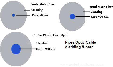
 The
new transatlantic cable will have the capacity for 200,000 simultaneous
online movie downloads.
The
new transatlantic cable will have the capacity for 200,000 simultaneous
online movie downloads. Robotic fiber positioners for dark energy instrument
A new instrument on the 4m Mayall Telescope at
Kitt Peak National Observatory will use 5000 robotic fiber positioners
to create a 3D redshift map of the universe to study dark energy.
13 July 2016, SPIE Newsroom. DOI: 10.1117/2.1201606.006531

The initial discovery of an accelerated universe in the late 1990s1,2
spurred scientific efforts to understand the underlying mechanism of
this new phenomenon. It is now well established that the so-called dark
energy, which drives the acceleration, accounts for about 70% of the
energy density of our universe. But we have yet to uncover the nature of
dark energy, nor do we know how it has competed with gravity over time
to shape the structure of our universe.
In an attempt to answer these questions, the Dark Energy Spectroscopic Instrument3, 4
(DESI) will conduct a large redshift survey and compile a 3D map of the
universe reaching to redshift 3.5 (23 billion light years) over more
than a third of the sky. By measuring the light spectra of more than 35
million galaxies and quasars, DESI will be able to precisely measure the
expansion history of the universe. DESI will also use the growth of
cosmic structure to study the properties of gravity, neutrinos, and the
inflationary epoch of the early universe.
The order-of-magnitude advance over previous redshift surveys5
will be achieved using 5000 robotically controlled fiber positioners
feeding a collection of spectrographs covering the wavelength range from
360 to 980nm. During each observation, light from 5000 galaxies will be
received by individual 107μm-diameter optical fibers. The closely
packed robots will position the fibers so that each captures the
spectrum of a single galaxy or quasar that we will then analyze using
spectrographs. The robots are designed to position the fibers precisely
and quickly, allowing rapid reconfiguration of the entire field for each
observation. This is critical in order to achieve our goal of
completing the survey within five years.
In test measurements, fiber positioners
consistently locate their fiber on target with an RMS accuracy better
than 5μm. To verify positioning, the fibers are back-illuminated after
each move, and their actual positions are measured by an on-axis CCD
camera located in the central hole of the primary mirror.
From the fiber plane image taken after the robots
complete positioning, we calculate the offset of the actual position of
the fiber from its desired position. These offsets are then fed to the
computer controlling the fiber positioners to enable correction. We
achieve the final accuracy iteratively. Typically, the first (blind)
move positions fibers within 50μm of the target position. Two subsequent
moves are sufficient to achieve micron precision.
The positioners have eccentric axis kinematics and are sized for a 10.4mm center-to-center pitch (see Figure 1).
Actuation is achieved by two 4mm-diameter DC brushless gear motors
(manufactured by Namiki Precision Jewel Co., Japan). The control of the
motors is handled by a small electronics driver board attached to the
rear (see Figure 2).
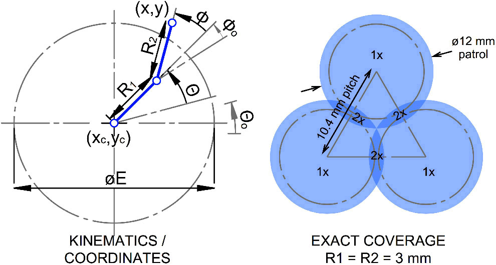
Figure 1. Left: Eccentric axis (Θ–Φ) kinematics. Whenever the Φ arm (R2)
is retracted within the dashed circle E, the positioner is guaranteed
free rotation about Θ without obstruction from its neighbors. Right: The
patrol region (the area within which every point can be reached by the
robot) coverage extends beyond the pitch. This assures complete coverage
but requires implementation of collision avoidance algorithms in the
move control software. R1, R2: Kinematic lengths of the Θ and Φ arms. xc, yc: Center of robot. x, y: Position of fiber. Θo, Φo: Home positions. 1×, 2×: Coverage by a single positioner and two positioners, respectively.
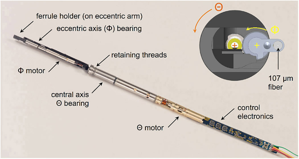
Figure 2. DESI (Dark Energy
Spectroscopic Instrument) 10.4mm pitch Θ−Φ fiber positioner. The centers
of the two axes are indicated on the insert (top right).
This board hosts a Cortex microcontroller running
custom firmware that provides CAN (controller area network)
communication, sends pulse-width-modulated signals to digital switches
for motor control, and provides telemetry functionality. Figure 3
shows a block diagram of the control electronics. The electronics board
is connectorless. The firmware contains an integral boot loader so that
after initial JTAG (an IEEE testing and interface standard)
programming, subsequent reprogramming can be performed remotely via the
CAN bus command lines. This feature allows full access to the
microcontroller while minimizing the wire connection count.
Electrical connection to each positioner is by a
single five-wire assembly that connects to an interface board. In
addition to power and CAN communication, each positioner receives a
synchronization signal to facilitate easy coordination of the motion of
multiple positioners.
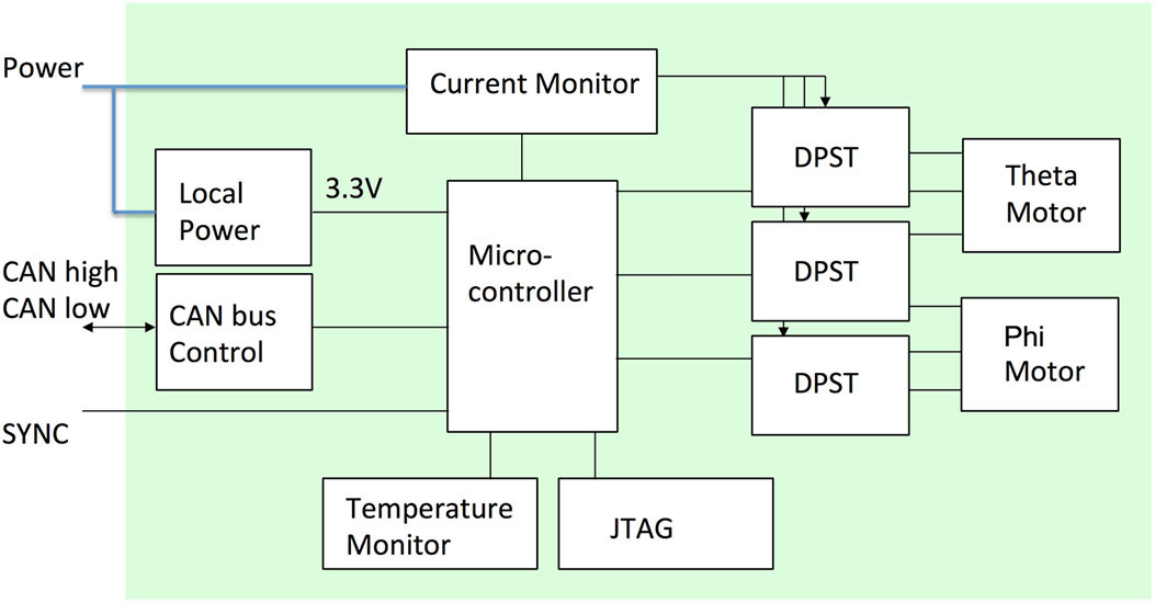
Figure 3. Local electronics of
the fiber positioner. Power is directed to the motors via digitally
controlled double-pole single-throw (DPST) switches. Monitoring of local
temperature and motor currents is provided. CAN: Controller area
network. SYNC: Synchronization. JTAG: IEEE testing and interface
standard.
Each positioner is uniquely addressed by an ID
number, and can be physically placed anywhere on the CAN bus. Groups of
positioners are connected in parallel, and in any order, to simple
two-line power and signal rails. Power to the electronics is shut off
when the positioner is not operating to reduce the heat load on the
focal plane.
Extensive tests have shown that the positioners are
fast (180°/s), accurate, and robust (tested to 400,000 reconfigurations
with no degradation in performance). A total of 20 machined parts and
10 fasteners go into the assembly of a positioner. Most of the research
and development was performed at Lawrence Berkeley National Laboratory,
with production of 5000 positioners now under way at the University of
Michigan. The assembly is done in stages, each positioner undergoing
quality control and testing.
After six generations of prototypes, the DESI fiber
positioners are now at a mature stage and ready for mass production.
Our tests show that they perform well and fulfill all specifications. A
first on-sky test will be performed in September 2016 with a small-scale
instrument (ProtoDESI), which tests various elements of DESI. At the
same time, the first DESI subassembly will be populated with 500
positioners and tested. By fall of 2018, the remaining positioners will
have been produced, tested, and installed before shipment to Kitt Peak
National Observatory. First light for DESI is expected in the winter of
2018/19, followed by a five-year survey in which, night after night, the
robots will reposition, enabling the instrument to collect an
unprecedentedly rich redshift sample for the study of dark energy.
________________________________________________________________________________
Remote Sensing
Calibration of airborne water reflectance measurements

Studying the water quality of
large lakes is a challenging task. For instance, collecting water
samples is time-consuming and insufficient for studying the
microproperties of water for a whole lake. In recent years, airborne and
spaceborne remote sensing techniques have been developed to overcome
this issue. From high altitudes, spectrometers can thus be used to
capture information (relevant to the study of bodies of water) over
large areas. Indeed, it is now known that several factors related to
water quality (e.g., the presence of phytoplankton or the concentration
of colored dissolved organic matter) can be assessed from the spectral
reflectance (i.e., the amount of radiation reflected) of the water.
In
a joint effort to study both Lake Geneva (Switzerland) and Lake Baikal
(Russia), several Swiss and Russian institutions have founded the
so-called Leman-Baikal project. As part of this work, between 2013 and
2015, scientists collected water samples, in situ hyperspectral data
(using a WISP-3 instrument from Water Insight and a RAMSES radiometer
from TriOS), and airborne hyperspectral data (using a Headwall Photonics
Micro-Hyperspec visible/near-IR sensor) to perform a large-scale
water-quality assessment of both lakes (see Figure 1).
A calibration procedure, however, is still needed so that data from the
pushbroom airborne sensor can be made to match the ground (i.e., in
situ) spectra. Only then will the airborne data be suitable for
large-scale analyses. Methods that have been developed so far for this
purpose, however, rely on additional onboard equipment,4 or they require the use of concurrent ground measurements.
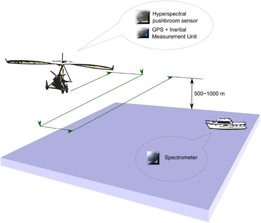
Figure 1. Schematic
illustration of the Leman-Baikal project acquisition campaign. At a
given time, an ultralight trike—equipped with a hyperspectral pushbroom
sensor—flies over a point of interest. In situ data is simultaneously
acquired (from a spectrometer on a boat) for the same point of interest.
GPS: Global positioning system.
We therefore propose a new, fully unsupervised
calibration procedure for the retrieval of water-leaving reflectances
from an airborne hyperspectral pushbroom camera.5
We have specifically designed this procedure so that we can deal with
all the inherent (i.e., noise and spectral smile) and external (e.g.,
contributions from the Sun, sky, and atmosphere) sources of error. We
can thus transform the output of the sensor into digital information and
subsequently into a unit-less measure of remotely sensed reflectance.
In particular, we propose new methods to correct the spectral shifts
induced by smile—a phenomenon that arises with pushbroom hyperspectral
sensors because the projection of the radiation from the dispersive
element onto the CCD array is distorted (in the shape of a smile) and
thus causes spectra collected in pixels from the same scan line to be
misaligned with respect to wavelength—or by moving dispersive elements
inside the sensor, and to scale data to reflectance.
To perform our spectral calibration, we rely on the
presence of the dioxygen absorption peak (around 760nm) in our
measurements. In our approach, we compute a signal—which represents the
fast variations (‘high frequencies’) within the spectrum—for each of two
spectra that we wish to align (i.e., with respect to their
wavelengths). We obtain this signal by dividing the original spectrum by
a smoothed version of it. The high frequencies signals therefore
highlight absorption peaks, especially the atmospheric absorption peak:
see Figure 2(a).
We then use an elastic matching algorithm (dynamic time warping) to
establish a band-to-band correspondence between the two high frequencies
signals. This correspondence can then be used to warp one signal (align
it bandwise) with the other signal. An example result is shown in
Figure 2(b).
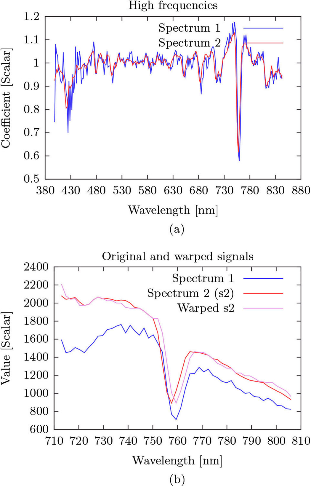
Figure 2. Illustration of the
spectral-shift removal process. (a) Signals of the high frequencies
(fast variations) in the spectra are obtained by dividing the original
signals by their smoothed versions. The high frequencies of the two
spectra, however, are misaligned. (b) Dynamic time warping (an elastic
matching algorithm) is then used to align the spectra. In this example,
the band-to-band correspondence is used to stretch spectrum 2 into new
warped spectrum with peaks that are aligned with those of spectrum 1.
Once the data has been filtered to remove noise and
smile, we process it further to mitigate the effects of
surface-reflected glint and to scale it to reflectance. The
water-leaving radiance is supposed to be negligible in the near-IR
(NIR). We therefore compute the correlations between the data from
different bands for a deep-water area,6
to reduce the impact of glint. We then measure an area of vegetation on
the shore and assume that its NIR reflectance is close to 50%. Although
the NIR reflectance of plants can vary substantially, our assumption is
a reasonable approximation of the real reflectance for a heterogeneous
area of healthy vegetation. By using a Spectralon (a unit-reflectance
panel that exhibits Lambertian behavior), we can estimate the
band-to-NIR transmittance ratio for each band of our camera. All the
transmittances can then be computed by simply scaling the NIR digital
number, collected with the Spectralon, to 50% reflectance. If this
scaling factor is inappropriate, we can determine a better factor from a
different ground measurement. At this point in our technique the method
becomes supervised.
To assess the performance of our calibration
process, we computed spectra for four sample points near the mouth of
the Rhône river in Lake Geneva and for four points in the Selenga Delta
of Lake Baikal. We obtained these measurements from low altitudes
(≤700m), which means that they are relatively unaffected by atmospheric
scattering. We also compared this data with in situ spectra that we
collected using the WISP-3 and RAMSES instruments. Both our calibrated
airborne data and our in situ data are plotted in Figure 3
for one of the Lake Geneva sites. We find a good similarity between the
calibrated and in situ data for all eight test points, with an average
correlation of 0.976.
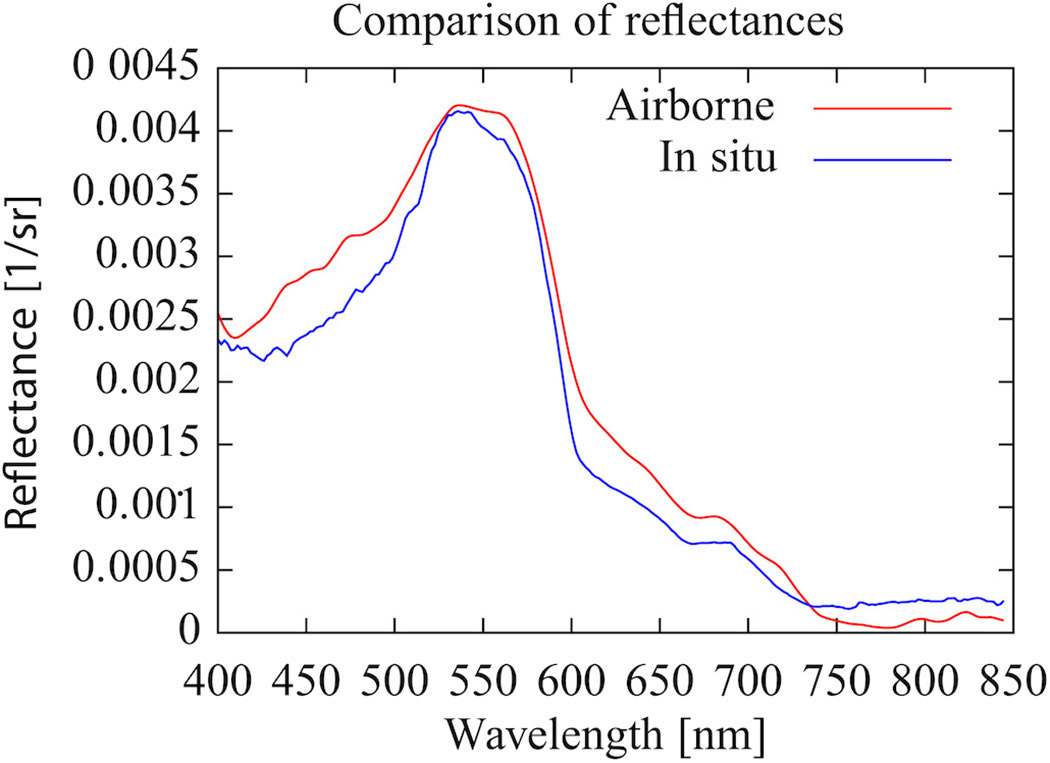
Figure 3. Comparison of a
calibrated airborne spectrum and an in situ spectrum for a location in
Lake Geneva (46.40860°latitude, 6.84326° longitude). sr: Steradian.
In summary, we have designed a self-calibration
algorithm, to transform sensor digital numbers to reflectance
information, for an airborne pushbroom hyperspectral camera. With our
algorithm we efficiently mitigate the effects of noise, spectral smile,
as well as external parameters such as glint and atmospheric scattering.
Our calibrated water-leaving reflectance outputs show good similarity
to simultaneously obtained ground measurements.5
In our ongoing work, we plan to focus on finding an efficient,
image-based atmospheric correction algorithm to calibrate spectra
obtained from higher-altitude flights.
_________________________________________________________________________________
Using ordered nanostructures on optical fiber tips as molecular nanoprobes

Since the development of an enzymatic electrode in 1962,
biosensors have been proposed for a range of applications (including
healthcare monitoring, clinical analysis, drug development, food
monitoring, homeland security, and environmental monitoring). Indeed, in
recent years, ever more powerful analytical and diagnostic tools have
been continuously demanded in the healthcare and pharmaceutical sectors,
i.e., for the identification of diseases and for the detection of
target biomolecules at very low concentrations, at precise locations
that are often hard to reach. New technology-enabled approaches are
therefore required for the development of ‘smart needles’ that have
unprecedented functionality, integration and miniaturization levels, and
that can be used to monitor clinically relevant parameters in real
time, directly inside the human body.
Optical
fibers (OFs) are unrivaled candidates for such in vivo point-of-care
diagnostics. This is because of their intrinsic property of conducting
light to a remote location, as well as their microscopic light-coupled
cross section, ultrahigh aspect ratio, biocompatibility, mechanical
robustness/flexibility, and easy integration with medical catheters and
needles. The intriguing combination of on-chip nanophotonic biosensors
and the unique advantages of OFs has thus led to the development of
so-called lab-on-fiber technology (LOFT).
Before LOFT platforms can be definitively established, however, there
is one main issue that needs to be addressed, namely, the lack of
stable, effective, and reproducible fabrication procedures that have
parallel-production capability.
To date, many prestigious research groups in the
photonics community have focused their efforts on addressing the major
challenge of matching the micro/nanotechnology world with that of OFs.
To further that pursuit and to fabricate regular patterns on an OF tip,
in this work we propose and demonstrate a novel lithographic approach
that is based on particle self-assembly at the nanoscale.
By exploiting the extreme light–matter interaction that can be achieved
when nanostructures are used, we have successfully used our decorated
fiber tips as surface-enhanced Raman scattering (SERS) substrates. Such
platforms thus enable the realization of ultrasensitive tools for in
vivo molecular recognition.
In our approach (see Figure 1),
we achieve the nanopattern by assembling polystyrene nanospheres (PSNs)
at the air/water interface (AWI), which leads to the formation of a
monolayer colloidal crystal (MCC). To produce floating MCCs, we drop an
alcoholic suspension on a water surface. The difference in surface
tension of the two substances causes the alcohol to spread quickly. The
PSNs are thus pushed onto the AWI, where—through collective motion and
capillary force—they self-assemble. To achieve the final transfer of the
nanopattern onto the fiber tip, we use a simple dipping method to
achieve the final transfer of the nanopattern onto the fiber tip, i.e.,
we lift part of the MCC island that is floating on the water surface
onto the fiber.
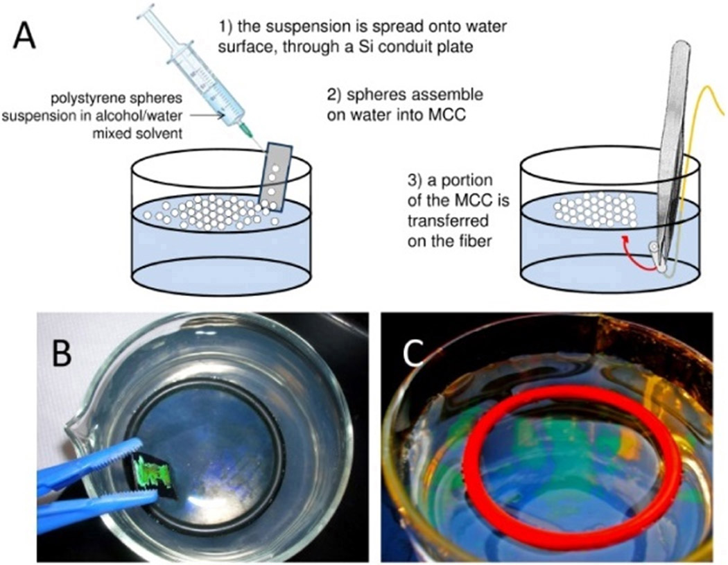
Figure 1. (A) Schematic
representation of polystyrene nanosphere (PSN) assembly at the air/water
interface (AWI), which leads to the formation of a monolayer colloidal
crystal (MCC), as well as subsequent deposition on the fiber.
Photographs of (B) the equipment used for the PSN self-assembly at the
AWI, where the silicon (Si) conduit plate is partially immersed in the
water (as indicated by the bright green color caused by the presence of
the packed nanospheres) and (C) the MCCs (which appear green because of
light diffraction) floating on water.
By applying further treatments to the MCCs, we can
efficiently produce different nanostructures (with completely different
morphological features), as shown in Figure .
We obtained a close-packed array of metallo-dielectric nanostructures
by simply depositing thin gold overlays on the uncoated fiber/MCC
assemblies. We also produced arrays of gold triangular nanoislands by
removing the metal-coated spheres. Furthermore, we can easily obtain
sparse arrays if we use oxygen plasma etching on the uncoated fiber/MCC
assemblies to reduce the PSN size. Holey gold nanostructures can be
obtained—through PSN removal—from the sparse arrays. In our work, we
have also verified the repeatability of our process (see Figure 3) and have thus demonstrated the effectiveness of our proposed fabrication route.
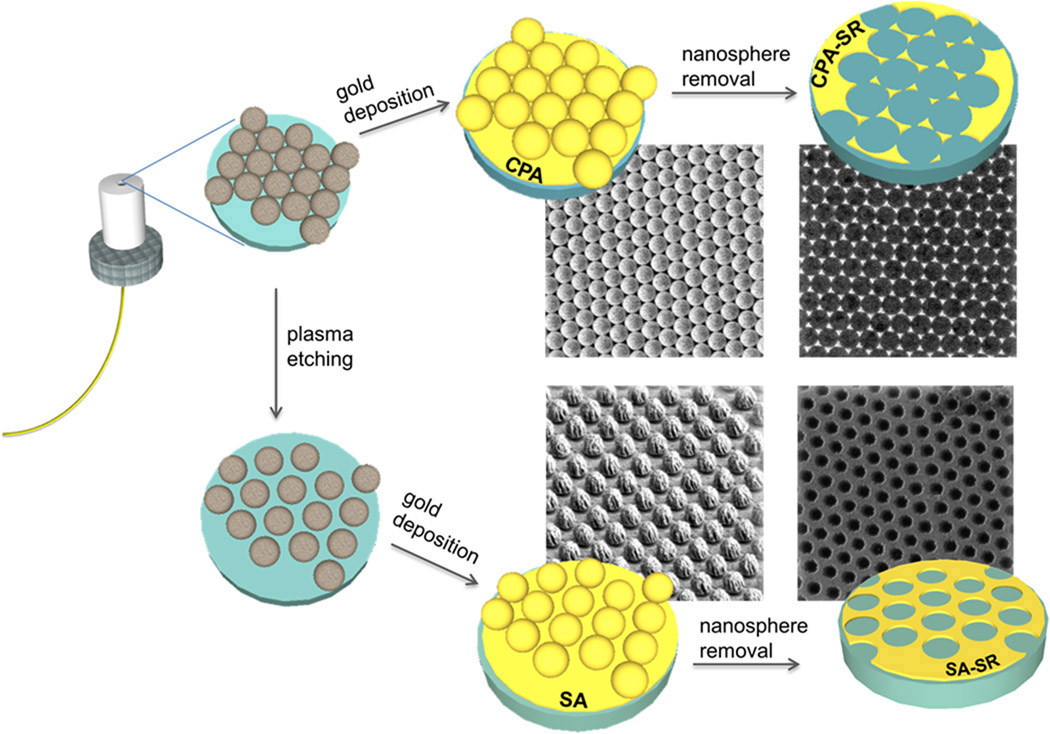
Figure 2. Schematic
illustration of the fabrication steps used to realize different periodic
structures on the optical fiber. CPA: Close-packed array. SA: Sparse
array. SR: Sphere removal. The inset shows scanning electron microscope
(SEM) images of the fiber facet for the corresponding fabricated
structures.8

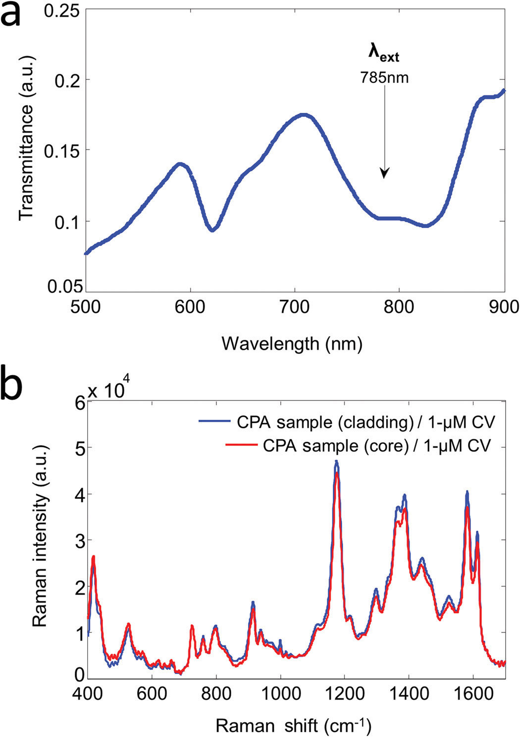
Figure 4. (a) Transmittance spectrum of the CPA sample (with a diameter of 1000nm), which exhibits a plasmonic resonance at 800nm. λext:
Excitation wavelength. (b) Surface-enhanced Raman scattering spectrum
obtained from 1μM crystal violet (CV). a.u.: Arbitrary units.
The kinds of complex, nanoscale, metallo-dielectric
structures we have produced can trigger interesting plasmonic phenomena
(with strong field localization) and can thus enable the development of
advanced platforms for biosensing applications.In our study, we conducted SERS measurements (in which illumination and
collection of the scattered light were made externally to the fiber
tip) to demonstrate that our decorated fiber tips can be used
efficiently as repeated SERS substrates. In these tests, we detected the
benchmark molecule (crystal violet) at a concentration as low as 1μM
(see Figure 3).
In summary, we have developed a simple and
cost-effective self-assembly approach for the integration of functional
materials (at the nanoscale) on OF tips. Our methodology thus provides a
valuable tool for the development of advanced OF bioprobes. In
particular, we have demonstrated the fabrication of reproducible SERS
fiber tips that can be used to detect a benchmark molecule at a very low
concentration. We now hope to drive the exploitation of this promising
technology for practical scenarios. Specifically, we will address
important issues such as the identification of suitable methodologies
for the excitation and collection of Raman signals with the same
patterned OF.
High Tech Robotic Hand Holding a Bundle of Fiber Optic Wire Cable - Communications Industry Technology Concept.
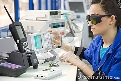

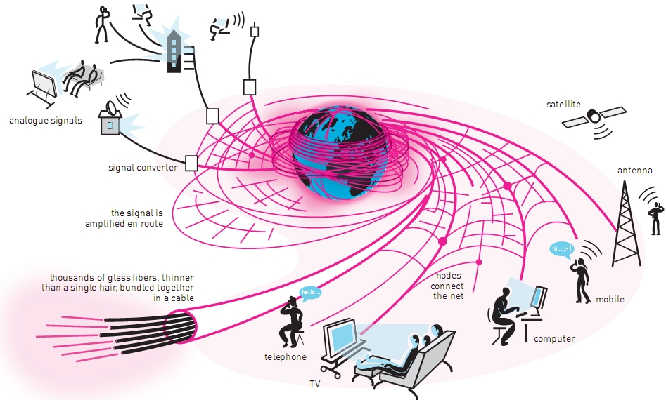


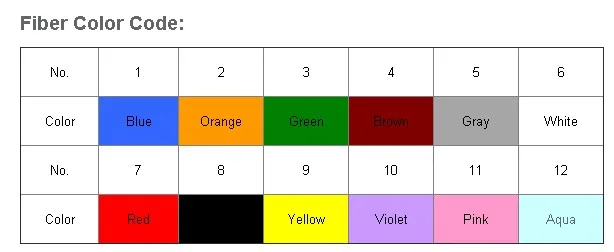
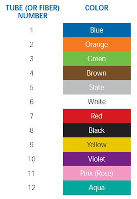
________________________________________________________________________________
Miscellaneous lightning lights
Operational Modes After studying the types of stage lights in a previous article, let us learn more about the various methods of controlling lighting. If you often come across the term Operational Mode on the specification of lighting but confused with its meaning, this article is right for you. Operational Mode is a mode of operation that can be executed to control the fixture. There are many aspects that can be controlled in lighting, such as lighting direction, the width of the diameter of the shot (beam angle), the color, the speed of change of color, dimming, strobing, as well as other effects. There are several ways of control (Operational Mode) to control lighting, including: Manual / Remote Control The first way is to manually course. Referred manually is that you have to approach the lighting fixture to change the settings manually. But as technology develops, in today's world almost all can be controlled remotely or automatically, unless of course follow spot that requires the operator to manually direct the spotlight to an object. To facilitate manual control from a distance, some lighting is now equipped with a remote function that uses radio frequency analog for controlling simple aspects of the lighting for example a color change, dimming, strobe effects and some other functions. Auto / Sound active sound active mode is the mode most often used by the venue owners who want lightingnya fixture featuring light show but do not have a lighting operator. By activating this mode, lighting you can follow the music / beat song that is being played. Master / Slave Master / Slave mode of operation in which the fixture is one (slave) set to follow the show or mode of operation that is running on the other fixture (master). This mode is typically used by light designer to run a simple light show and wanted some fixturenya actively use the same mode. So just by controlling the master fixture, all the other slave fixture can move together.
DMX512DMX512 (Digital Multiplex) is a communications protocol that enables access control of various parameters on a lighting, whether it dimming, color, gobo, direction of movement of the moving head, and a variety of other specific parameters on a fixture. To control the fixture DMX <required controller which is not only just a hardware / mixer, but also in the form of software. By using the software, the ability to control the lighting system is very complex because it is not limited to the number of buttons on a hardware mixer. Even DMX software can now be controlled using MIDI controller general. A fixture that has no DMX features can not be controlled in detail to produce a more complex light show. One of the DMX software that you can use is MyDMX2.0 Art-Net / Kling-Net protocol Art-Net and Kling-Net is generally used to control the LED panel to display a particular sequence or animation. Methods for controlling the LED panel is also called Pixel Mapping. Art-Net itself is basically a protocol that was developed to transfer data DMX via UDP (User Datagram Protocol) as used on Internet communication protocol via ethernet cable. While Kling-Net is a protocol developed by ArKaos to distribute video in real-time to the LED panels which have been prepared on a large scale. To control the lighting with Kling-Net protocol, can use software GrandVJ and MEDIAMASTER of Arkaos.
ILDAILDA (International Laser Display Association) was originally a light international association for designers, especially laserist (the term for a lighting designer who focuses on laser). ILDA then developed a special image format for transferring image / picture from a controller to the laser fixture. Since then, came the ILDA format designed specifically for laser use. Laser projector that has operational ILDA mode can be custom programmed to display images even any animation. One of the most powerful software makers to control the laser ILDA is Pangolin.
kind type of lighting lamps


___________________________________________________________________________
Working Principle TelevisionThe workings of a TV station first starts of the Department of Programming. This is the planning department and determine what programs will be delivered, at what time, and who the target audience. Then
the program was whether it should be made own inhouse, outsourced,
purchased from a local PH or must be imported from abroad. If purchased from abroad, the program was in the form of a cassette or in the form of a live broadcast (live). Progam imported in the form of cassette tape example is the film
series The A-Team, Smallville or Mc Gyver, while imports of live
programs such example is world cup football, professional boxing or car
racing F1.
If programs that have been selected and the broadcast schedule has dutentukan, then the Sales & Marketing that will market / sell it to prospective advertisers. Time slots are available for ads then given the price (rate card), while the type of ad that can be offered in the form of video, graphics, animation, running text, built-in or ad blocking time. It all depends on the agreement between the two parties (advertisers and TV station operator).
If the program itself must be made in-house, then the production will then draw up crew, schedule and produce programs that targeted a predetermined time. Production can be done in the studio or outside the studio, depending on the type of program being made. After so (in the form of a cassette tape or a disk file) The next step is the process of Post Production (Editing, Graphic and Quality Control). When it has escaped from the Quality Control means the program was ready to be served, and the program was later sent to playout to put in the waiting list (Play List). Later, in hours, minutes and seconds that have been determined, the program will run itself automatically on the orders of On-Air Automation software.
On-Air Automation works based data entry entered by Traffic section. The data in the entry, for example: the program title, duration, hours, minutes and seconds when the program should appear on the screen. If facilities are available, the data can also contain when running text, graphic or animated ads must appear together with the program (this facility is called the Secondary Event). Traffic section is typically below Sales with the aim to facilitate the coordination and control of ad serving. Because this berakitan closely with billing issues and payment for advertisements. Traffic or traffic control program and this ad is quite complicated, as it involves many parties (Programming, Sales, Finance and Engineering) that required special software to help simplify the technical-operational.
When everything is neatly arranged and later in the run, then playout automatically deliver the program and advertising it in sequence according to the schedule that has been arranged in the Play List. Audio-video signals coming out of playout and then selected by the Master Switcher to be sent to the transmitter to be emitted. In many cases the location of the transmitter is often far outside the studio, so we need a tool that serves ntuk distribute the signal from the studio to the transmitter. The tool is then called by STL (Studio to Transmitter Link) as shown in the diagram below.

In
drawing up the program sequence is often a time slot for the live
broadcast (live), either from within or from outside the studio. While
the live broadcast is usually the time is often uncertain, in a sense
can be forward or backward a few minutes or seconds. Therefore, in the On-Air Automation software generally has available
facilities capable of adjusting the reciprocation of serving time live
broadcast this program.The
live broadcast from outside the studio generally use fiber optic lines,
satellite or microwave links as a means to transmit signals from the
location to the studio. The
signals coming from the outside have been through Routing Switcher and
then be synchronized in advance with the existing signaling standard
that is in the studio. A device that serves to synchronize the video signal is called the Frame Synchronizer. Furthermore, to measure the quality of signals from the outside it is
used in the form of video monitoring equipment Waveform and Vectorscope.
The live broadcast from the studio for example is a news broadcast, interview or dialogue. In the news broadcasts are often interspersed with live reports from the location. Then the signal from this location should be sent first to the studio, then combined with a news reader (sometimes inserted text and the pictures are graphic), and then forwarded to the Master Switcher for insertion of logos, running text or animated ads (if any) and subsequent output of Master Switcher is sent to the transmitter.
If the size of the studio was big enough then it could be used to produce entertainment programs such as talk shows, quizzes, contests / live music or other events rather colossal. But it all depends on the vision and mission of the TV station itself. In some TV stations, studios for entertainment programs as it is generally separate from the studio to broadcast news, so there is more than one studio to produce a different program. But in some of the many TV stations also encountered only one studio to produce various kinds of programs. The aim is for efficiency. That is, efficient in terms of investment tools, the room and the number of personnel to operate it.Studio are often used for recording purposes (taping). The tape later in the process in the ranks of Post Production to undergo the process of editing. For example, the pictures do not need to be disposed of, a weak voice amplified or too strong is reduced, then given written or graphic to look more attractive, or by insertion sound (dubbing / voice over) when necessary. Once that process is completed then all the material submitted to the Quality Control department for examination quality. When you have passed the QC then shipped to Play Out to put in the waiting list (Play List). At a predetermined time, the program will then automatically broadcast sendirir behest On-Air Automation software.
INTERCOMInside the studio, a lot of parties involved in the production of a program of activities, namely:01. Producer02. Program Director03. Floor Director04. Anchor / Host05. cameramen06. Switcherman07. Audio Engineer08. Lightingmen09. CG / Graphic Operator10. VTR / Record & Play Back Operator11. Operator TelePrompTer12. Technical Support13. Master Control
To all the personnel is always involved in a program of production activity in the studio. Especially for the live broadcast program, the atmosphere of the production activities generally very noisy, it works very fast rhythm, full of pressure and a decision should be taken on the spot, but the error should be minimum. You can imagine what it would be if there were no channels dedicated communication between one another. All the personnel concerned would be shouting to convey meaning. While the rest of the band, with the interests of others, will also do the same thing. Then the atmosphere will be very noisy and rowdy. Well here Intercom is required, Intercom main function is to be a channel of communication that is orderly and purposeful. Conduct within the meaning communication can take place alternately, while the focus in the sense that there are some channels that can be selected for komuniikasi in groups with different interests. For instance:1. Producer only spoke to Anchor / Talent through channels Interrupt Program.2. Program Director spoke with cameramen through the channel-1.3. Producer speak with Floor Director through the channel-2.4. Program Director spoke with Audioman, Graphic, MCR and Technical Support via the channel-3.5. While the channel-4 is used for sharing (Party Line).

The communication channel is divided multiple channels for different purposes.
That's it. So with this Intercom communication in the studio will be orderly and purposeful. Intercom is also often used for communication between the studio and the location outside the studio, where an event is in progress. In order for this communication still takes place in an orderly and purposeful, required an interface between the Intercom with telephone lines. With this interface, the crew inside the studio could communicate with the crew who are outside the studio through the telephone network to communicate via Intercom like usual. One product interfaces such example is ClearCom type AC-701 (see picture 1).Intercom relationship from Producer to Talent can also take place wirelessly using a transmitter and receiver ClearCom ClearCom PTX2 PRC2 (see picture 1), and many more variations intercom products that can be selected to meet very specific needs that might be in their respective studios. Figure 2 shows another example diagram Intercom 4 channels are very commonly used in News Studio.For more complex intercom network are strongly advised to use the intercom MATRIX kind that works like a PABX telephone, where there is one central, and there are many Remote Station. Each Remote Station Remote Station can contact another simply by pressing certain buttons, like a push button telephone. Examples of products along varasinya Intercom can be seen in more detail in the Product Intercom.
That's it. So with this Intercom communication in the studio will be orderly and purposeful. Intercom is also often used for communication between the studio and the location outside the studio, where an event is in progress. In order for this communication still takes place in an orderly and purposeful, required an interface between the Intercom with telephone lines. With this interface, the crew inside the studio could communicate with the crew who are outside the studio through the telephone network to communicate via Intercom like usual. One product interfaces such example is ClearCom type AC-701 (see picture 1).Intercom relationship from Producer to Talent can also take place wirelessly using a transmitter and receiver ClearCom ClearCom PTX2 PRC2 (see picture 1), and many more variations intercom products that can be selected to meet very specific needs that might be in their respective studios. Figure 2 shows another example diagram Intercom 4 channels are very commonly used in News Studio.For more complex intercom network are strongly advised to use the intercom MATRIX kind that works like a PABX telephone, where there is one central, and there are many Remote Station. Each Remote Station Remote Station can contact another simply by pressing certain buttons, like a push button telephone. Examples of products along varasinya Intercom can be seen in more detail in the Product Intercom.

One example configuration of Intercom in the studioStudio: Video Work FlowInside the studio there are three main components, namely: Cameras, Monitors and Video Switcher. The
camera function to take a picture, then the results can be viewed on
screen, while Switcher serves to switch (toggle) images coming from
cameras 1, Camera 2, Camera 3 and so on. The output is then sent to the transmitter or can be recorded onto a video tape recorders or video servers. This is the most basic principle of a working mechanism in the studio with a number of cameras is more than one. Question: why did it take more than one camera? Due to the many camera can image objects taken from several angles at the same time, so shooting becomes more effective. That is why Swicther required in multi-camera systems that capture images from one corner to the other can be changed quickly.Each camera was given the Monitor. The aim is that Switcher operator can easily identify where the camera is ready and the camera is not. The camera is not ready usually still perform adjustment (pan, tilt, zoom and focus) on an object image that is being taken. A Program Director (PD) may ask the cameraman, via Intercom, to direct the camera to a certain object. Furthermore,
through the Monitor-Monitor in the Control Room, PD can see whether an
image taken by a cameraman it is appropriate that he wants to or not. If not, then he could ask again for Cameraman perform image adjustment again until he meant fulfilled. That is why Intercom become a vital means of communication in the Studio.Switcher
generally equipped with the Monitor PREVIEW which serves as the monitor
shortly before the image is shown, while the image is being aired can
be seen through the Monitor PROGRAM. Video
output of PROGRAM generated by Switcher, further in-stribusi-kan by the
VDA (Video Distribution Amplifier) to multiple destinations. Among them are to the transmitter's emitted, to the Video Server to be recorded and to Floor Monitor (see picture (1) below). Floor
Monitor placed in the studio, and function like a mirror for the actor,
anchor or MC in action so that he can see for himself how it looks on
the screen.

Video flow diagram for a multi-camera studio basic level. Larger image.Based on experience, 3 pcs camera is the most optimal amount for studio news (News Studio). For most objects in the News Studio image can be more than one. For
example 2 Anchor reads news alternately, or one Anchor with one or two
resource persons, where objects pictures like this are relatively silent
(not move) and generally also be formal (sedentary), so 3 Camera rated
fit for cover image object like this.In stark contrast to entertainment programs such as Live Music, Contests or Fashion Show for example. Programs
like this picture many objects, move, move where and non-formal
(shooting could be from the bottom, from the top or side). Thus the number of cameras needed for entertainment programs like
these become more numerous, so it takes Switcher by the number of input
ports is more too.In
a program, an image originating from camera alone to be sufficient,
because the information displayed would not be complete without the
addition of sufficient supporting data. The supporting data can be text or graphical images. That is why it takes a computer graphics and CG (Character Generator
letter generator = computer) to make a program in order to be more
informative and interesting.In
addition it also needed pieces of program (video clip) to be inserted
into the main program, where video-clip video has been deliberately made
in such a way is to complete the main program. That requires centrifuges video clip (playout system) for example is the Video Server. Generally
Video Server totaled 2 pieces that can be used interchangeably (A-B
Roll), or Video Server which one becomes a back up of the Video Server
to another. Video
servers are generally also equipped with an input port and perekamanan
software so that it can function as a recording device. First
video recording device is the most popular VTR (Video Tape Recorder),
where the video signal is stored in the magnetic strip. But now a store video of the more popular hard drives, solid state
disk (SSD) or a memory card, so that the computer or server into a tape
recorder or a video player that is dominant today.From
the above discussion it became clear that in addition to the purposes
of live broadcasts, studio equipment can also be used to record programs
(taping). The recorded signal does not always come from the studio, but it could also come from outside the studio. For
example, want to record live broadcasts Italian league football, which
once recorded the results will be aired the next day. Italian
League live broadcast can be obtained from the satellite using a
satellite dish and a receiver called TVRO (Television Receive Only). It is important to provide input port padaSwitcher as an entrance for the signal coming from the outside. And in addition to record signals from the outside, the input port can also be used for live broadcasts.
And what about the signal coming from the outside? Is not the signal from the outside it was definitely not in sync? Now that the synchronous signal from the outside it must be passed prior to the Frame Synchronizer (see the block in the image (2) blue). By a Frame Sync signal from the outside it will be captured and then digitally modified such that the vertical and horizontal position equal blanking / synchronous signal in the studio. In this way, the signal from outside the studio will always be in sync with the signal in the studio (existing).After all the signals are synchronized and how to equate the image quality of the three units of the Camera? Imagine if there are three cameras that take pictures of objects of the same. For example, the face image broadcaster. Camera-1's face capture broadcasters from the left, camera-2 from the right and the camera-3 from the front. It turned out that the results can vary. For example, broadcasters face from the left corner looks a little brighter, from the right corner while a little more contrast from the front slightly redder, and many other details that could reveal differences. So although the three cameras of the same brand and type, but the images produced can vary. This difference may not be so obvious, but when viewed through the measuring instrument then see the difference. This is because each of the cameras in the set individually using a separate monitor. And when combined in a single output screen will then see the difference. That is why it is advised not to take pictures the same object from two different cameras, because if there are differences between them will be easy to see. Also it is advisable to use a camera with the same brand and type, because if the brand / type of camera is different certainly the resulting image will be different. Unless the object image taken is different, because the two objects of different images must not be compared. So the differences will be very difficult to identify when an object image taken different.To overcome the problem of the difference is then used a device called a CCU (Camera Control Unit). CCU through this every time the camera can be set so as to produce bright, contrast and style / color that is really similar to each other. To help multi-camera setting is commonly used measuring devices Waveform and Vectorscope. Waveform to help measure the contrast and dark-bright image (Luminance), while Vectorscope is required to determine the amplitude and phase angle of the signal color (chrominance). The amount is enough for one course via Video Routing Switcher inputs of Waveform & Vectorscope can be changed easily. So Waveform & Vectorscope in addition to sets the camera at the same time also can be used to measure and monitor other devices such as: CG, Graphic, Server, Frame Sync and also Output Program [see picture (2)]In the picture (2) there is a large monitor screen. This is intended to reduce space requirements, given the number of monitors needed quite a lot so it requires a fairly large room. By bringing together these monitors into one screen, then the space requirement is much reduced. Besides the installation of a wide-screen (55-inch LED TV, for example) is practically also very easy. The price is now also relatively inexpensive. But for this purpose diperlukanMuti-Viewer, a tool that serves to display images of many inputs into a single screen. In the Multi-Viewer there is a facility to adjust the position of the image, the image area and the labels on every box image. In fact, there is also a facility to display Audio Level to monitor the audio output level.


There is one more thing that needs to be discussed further, which is about synchronization. When
Video Switcher move the input signal from the camera 1 to camera 2, for
example, what happens exactly when the switch is changed? Imagine,
when Camera 1 is doing the scanning, just as the scanning position
exactly the center of the screen, and then switch to move to the Camera
2. Whereas Camera 2 were taking pictures of objects to another. So the picture is half the screen remainder of Camera 1 had continued to go? Well on conditions such as this that will cause the displacement of the image from camera 1 to camera 2 becomes "jumping". Then jumping problem is then solved in a way: the switch will move only when scanning in the position of the vertical blanking.The
second question is: when the camera 1 is in the vertical blanking
position, whether at that moment the camera 2 in the position of the
vertical blanking too? The answer is no, because we do not know. Therefore,
the switch will move when the camera 1 is in the vertical blanking
position and wait until the camera 2 in the position of the vertical
blanking well. And
because of the position of the vertical blanking both cameras are not
the same (no sync), then transfer from camera 1 to camera 2 had to be
delayed. The length of this delay time is half the frame (20 milliseconds) maximum. During
a very short delay, the image from camera 1 will be frozen for a moment
(freze) before being replaced by images from the camera 2. This
incident took place in such a short (max 20 milliseconds) so that the
effect is not so obvious. Therefore Switcher with such weakness is still widely used given the relatively cheap and its effect is not so obvious.In order to transfer images from camera 1 to camera 2 running smoothly, then each device must be synchronized. That is, the sync pulses in the two cameras must be the same. That
requires a signal generator synchronization (Synch Generator) where the
signal or the sync pulses may be further in-distribution-kan via Video
Distibution Amplifier (VDA) to all cameras and other devices, such as:
CG, Graphic, Server and Switcher ( consider the block in the image (2) which is green). Thus when the image is moved by Swicher from one input to another input displacement will go smoothly. For
all the devices are already using the same reference signal, so that we
can be sure that the position of vertical or horizontal blanking pulse
will always be the same.
And what about the signal coming from the outside? Is not the signal from the outside it was definitely not in sync? Now that the synchronous signal from the outside it must be passed prior to the Frame Synchronizer (see the block in the image (2) blue). By a Frame Sync signal from the outside it will be captured and then digitally modified such that the vertical and horizontal position equal blanking / synchronous signal in the studio. In this way, the signal from outside the studio will always be in sync with the signal in the studio (existing).After all the signals are synchronized and how to equate the image quality of the three units of the Camera? Imagine if there are three cameras that take pictures of objects of the same. For example, the face image broadcaster. Camera-1's face capture broadcasters from the left, camera-2 from the right and the camera-3 from the front. It turned out that the results can vary. For example, broadcasters face from the left corner looks a little brighter, from the right corner while a little more contrast from the front slightly redder, and many other details that could reveal differences. So although the three cameras of the same brand and type, but the images produced can vary. This difference may not be so obvious, but when viewed through the measuring instrument then see the difference. This is because each of the cameras in the set individually using a separate monitor. And when combined in a single output screen will then see the difference. That is why it is advised not to take pictures the same object from two different cameras, because if there are differences between them will be easy to see. Also it is advisable to use a camera with the same brand and type, because if the brand / type of camera is different certainly the resulting image will be different. Unless the object image taken is different, because the two objects of different images must not be compared. So the differences will be very difficult to identify when an object image taken different.To overcome the problem of the difference is then used a device called a CCU (Camera Control Unit). CCU through this every time the camera can be set so as to produce bright, contrast and style / color that is really similar to each other. To help multi-camera setting is commonly used measuring devices Waveform and Vectorscope. Waveform to help measure the contrast and dark-bright image (Luminance), while Vectorscope is required to determine the amplitude and phase angle of the signal color (chrominance). The amount is enough for one course via Video Routing Switcher inputs of Waveform & Vectorscope can be changed easily. So Waveform & Vectorscope in addition to sets the camera at the same time also can be used to measure and monitor other devices such as: CG, Graphic, Server, Frame Sync and also Output Program [see picture (2)]In the picture (2) there is a large monitor screen. This is intended to reduce space requirements, given the number of monitors needed quite a lot so it requires a fairly large room. By bringing together these monitors into one screen, then the space requirement is much reduced. Besides the installation of a wide-screen (55-inch LED TV, for example) is practically also very easy. The price is now also relatively inexpensive. But for this purpose diperlukanMuti-Viewer, a tool that serves to display images of many inputs into a single screen. In the Multi-Viewer there is a facility to adjust the position of the image, the image area and the labels on every box image. In fact, there is also a facility to display Audio Level to monitor the audio output level.
Pictures (2) video flow diagram for advanced multi-camera studio. Larger image.
In the picture (2) there is a PC for Teleprompter, a word-processing machines (text) where the output can be displayed to the screen placed in front of the camera. Above the screen is mounted translucent glass with a slope of 45 degrees so it does not block the camera lens but it also serves to reflect the text coming from the monitor screen. The reflection in the glass text is then readable by Anchor or Host. Teleprompter can stand alone or integrated with Automation News. Figure (3) shows the interconnection of a Teleprompter
In the picture (2) there is a PC for Teleprompter, a word-processing machines (text) where the output can be displayed to the screen placed in front of the camera. Above the screen is mounted translucent glass with a slope of 45 degrees so it does not block the camera lens but it also serves to reflect the text coming from the monitor screen. The reflection in the glass text is then readable by Anchor or Host. Teleprompter can stand alone or integrated with Automation News. Figure (3) shows the interconnection of a Teleprompter
Interconnection diagram Teleprompter
Studio: Audio Work FlowIn the studio making the audio signal is completely separate from the video signal. The video signal is taken using the camera while the audio signal is taken using a microphone. Microphone is a transducer that converts air pressure affecting the membrane in it into an audio signal. The resulting audio signal further strengthened, regulated and controlled via the Audio Mixer. The main output of the mixer further in-distribution-kan to multiple destinations through ADA (Audio Distribution Amplifier). One output is sent together with the video signal to the transmitter to be transmitted, while the other output is connected to Video Server A and B to be recorded along with the video signal at the time of taping, or taped to the Instant Replay for replay shortly after the record.There are two types of relationships from Microphone to Audio Mixer, namely wired and wireless. Wired (use cable) is generally used to connect Microphone position relative to stationary or rare move, while wireless (cordless) Microphone is perfect for that position are often on the move. There are two types of Wireless Microphone, the type held (handheld) and the type of Clip-On (clamped near the collar). Wireless Clip-On must be connected to a transmitter that is placed inside the Belt-Pack, and then beam the signal was captured by the Receiver (Rx) to then be connected to the input of the Audio Mixer.For monitoring purposes there are several Audio Monitor to be installed. One for the audio operator itself, one for video and another operator for the audience (Floor Monitor). One output is again connected to IFB (Intercom Fold Back) connected with the Ear Set is placed in the ear Anchor / MC / host. Thus, each person having an interest in the studio can hear what is going on so that they can act according to their respective roles.In some cases, when there are programs that require as background music, then the CD player needs to be available to meet that need. It is also necessary to broadcast the Telephone Hybrid that comes from sources that are outside the studio. Telephone Hybrid serves to take the voice signal flowing on telephone lines into audio signals to be more easily integrated into the Audio Mixer, and otherwise modify the audio signal from the mixer into a voice signal to match the telephone lines. The number of telephone lines coming into the Telephone Hybrid can be selected as needed, so that two (or more) sound sources can be displayed together with the sound Anchor, MC or Master of Ceremonies in the studio. Furthermore, when in Studio are fasilitasVirtual Set, the necessary audio delay which serves to delay the audio signal to be in sync with the video signals that were a result of the delay video signal processing and 3-dimensional graphics in the Virtual Machine Set.
Studio: Audio Work FlowIn the studio making the audio signal is completely separate from the video signal. The video signal is taken using the camera while the audio signal is taken using a microphone. Microphone is a transducer that converts air pressure affecting the membrane in it into an audio signal. The resulting audio signal further strengthened, regulated and controlled via the Audio Mixer. The main output of the mixer further in-distribution-kan to multiple destinations through ADA (Audio Distribution Amplifier). One output is sent together with the video signal to the transmitter to be transmitted, while the other output is connected to Video Server A and B to be recorded along with the video signal at the time of taping, or taped to the Instant Replay for replay shortly after the record.There are two types of relationships from Microphone to Audio Mixer, namely wired and wireless. Wired (use cable) is generally used to connect Microphone position relative to stationary or rare move, while wireless (cordless) Microphone is perfect for that position are often on the move. There are two types of Wireless Microphone, the type held (handheld) and the type of Clip-On (clamped near the collar). Wireless Clip-On must be connected to a transmitter that is placed inside the Belt-Pack, and then beam the signal was captured by the Receiver (Rx) to then be connected to the input of the Audio Mixer.For monitoring purposes there are several Audio Monitor to be installed. One for the audio operator itself, one for video and another operator for the audience (Floor Monitor). One output is again connected to IFB (Intercom Fold Back) connected with the Ear Set is placed in the ear Anchor / MC / host. Thus, each person having an interest in the studio can hear what is going on so that they can act according to their respective roles.In some cases, when there are programs that require as background music, then the CD player needs to be available to meet that need. It is also necessary to broadcast the Telephone Hybrid that comes from sources that are outside the studio. Telephone Hybrid serves to take the voice signal flowing on telephone lines into audio signals to be more easily integrated into the Audio Mixer, and otherwise modify the audio signal from the mixer into a voice signal to match the telephone lines. The number of telephone lines coming into the Telephone Hybrid can be selected as needed, so that two (or more) sound sources can be displayed together with the sound Anchor, MC or Master of Ceremonies in the studio. Furthermore, when in Studio are fasilitasVirtual Set, the necessary audio delay which serves to delay the audio signal to be in sync with the video signals that were a result of the delay video signal processing and 3-dimensional graphics in the Virtual Machine Set.
Audio flow diagram for a studio in general.
Studio to Transmitter Link (STL)The position of the transmitting antenna is most ideal in high places. The purpose is so that the radiation waves emitted radia can freely reach the widest possible area unobstructed. Because the working frequency of TV broadcasts are in the UHF band, so to get a better signal reception when the antenna is transmitting funds can see each receiver antenna (Line of Sight). To qualify for this ideal then needed a tower high enough to put an antenna on it. The higher the location of the transmitting antenna itself will be easily seen by the receiving antenna.But the height of the antenna tower also has its limits. Not only because of the higher prices that tower makain expensive, but the height of the tower is often limited by Regulation (local regulations). Because this case involves the beauty of the layout of the city or because of safety concerns local airlines. To solve the problem of this law then the antenna towers have to be placed in a rather high place in the suburbs. For instance Semarang. In Semarang TV towers almost all placed on a hill Gombel, because the land is rather high position so that the antenna TV receiver can easily see in this direction. Likewise, Napier, where many TV towers placed in Bili-Bili is located on the edge of town and land position pacaraan signal is high enough so that it can reach a very wide area.On the other hand, an ideal position for production equipment and studio is in town. Because the number of personnel involved in it so much more, and coordination with outside parties are also definitely easier. Therefore, the position between the transmitter and the studio have become no distance. Jaraknyapun often too close. In fact there are up to 20 km more. Now that the signal from the studio can be emitted by the transmitter takes a channel as a liaison. A conduit is then called by STL (Studio to Transmitter Link).There are three types of STL that can be selected, namely: microwave, fiber optic or satellite. The device is relatively expensive satellite and transponder rental price is also expensive. Fiber optic pemasangnnya very long and complicated licensing need to spread them along the pathway. So of the three options it is most often selected is a microwave, because microwave devices are relatively cheap price and time to install the relatively very fast.
Studio to Transmitter Link (STL)The position of the transmitting antenna is most ideal in high places. The purpose is so that the radiation waves emitted radia can freely reach the widest possible area unobstructed. Because the working frequency of TV broadcasts are in the UHF band, so to get a better signal reception when the antenna is transmitting funds can see each receiver antenna (Line of Sight). To qualify for this ideal then needed a tower high enough to put an antenna on it. The higher the location of the transmitting antenna itself will be easily seen by the receiving antenna.But the height of the antenna tower also has its limits. Not only because of the higher prices that tower makain expensive, but the height of the tower is often limited by Regulation (local regulations). Because this case involves the beauty of the layout of the city or because of safety concerns local airlines. To solve the problem of this law then the antenna towers have to be placed in a rather high place in the suburbs. For instance Semarang. In Semarang TV towers almost all placed on a hill Gombel, because the land is rather high position so that the antenna TV receiver can easily see in this direction. Likewise, Napier, where many TV towers placed in Bili-Bili is located on the edge of town and land position pacaraan signal is high enough so that it can reach a very wide area.On the other hand, an ideal position for production equipment and studio is in town. Because the number of personnel involved in it so much more, and coordination with outside parties are also definitely easier. Therefore, the position between the transmitter and the studio have become no distance. Jaraknyapun often too close. In fact there are up to 20 km more. Now that the signal from the studio can be emitted by the transmitter takes a channel as a liaison. A conduit is then called by STL (Studio to Transmitter Link).There are three types of STL that can be selected, namely: microwave, fiber optic or satellite. The device is relatively expensive satellite and transponder rental price is also expensive. Fiber optic pemasangnnya very long and complicated licensing need to spread them along the pathway. So of the three options it is most often selected is a microwave, because microwave devices are relatively cheap price and time to install the relatively very fast.
Figure (1): Three options STL, namely: (1) Microwave (2) Fiber Optic and (3) Satellite
In STL operation must be highly reliable, which means that the link should not be broken. Because if you break means broadcasts can not take place. Therefore STL to be made redundant. The goal is that when one link breaks it will replace the other link. Thus the reliability of the link really guaranteed. About SSL configuration is redundant, quite a lot of configurations that can be selected, namely:1. Configure two pairs of microwave link, A and B (A and B as playing as a back up)2. Configure 2 fiber optic link, A and B (A and B as playing as a back up)3. Configure as the main microwave and fiber optic as a back up4. Configuring the microwave as the main and satellite as a back up5. Configure as the main fiber optic and satellite as a back upConfiguration number (1) is a configuration that is most widely used by local TV stations, while the configuration of the number (4) of the most widely used by national TV station
In STL operation must be highly reliable, which means that the link should not be broken. Because if you break means broadcasts can not take place. Therefore STL to be made redundant. The goal is that when one link breaks it will replace the other link. Thus the reliability of the link really guaranteed. About SSL configuration is redundant, quite a lot of configurations that can be selected, namely:1. Configure two pairs of microwave link, A and B (A and B as playing as a back up)2. Configure 2 fiber optic link, A and B (A and B as playing as a back up)3. Configure as the main microwave and fiber optic as a back up4. Configuring the microwave as the main and satellite as a back up5. Configure as the main fiber optic and satellite as a back upConfiguration number (1) is a configuration that is most widely used by local TV stations, while the configuration of the number (4) of the most widely used by national TV station
Tidak ada komentar:
Posting Komentar