In fluid dynamics, wind waves, or wind-generated waves, are surface waves that occur on the free surface of oceans, seas, lakes, rivers, and canals or even on small puddles and ponds. They result from the wind blowing over an area of fluid surface. Waves in the oceans can travel thousands of miles before reaching land. Wind waves range in size from small ripples, to waves over 100 ft (30 m) high.
When directly generated and affected by local winds, a wind wave system is called a wind sea. After the wind ceases to blow, wind waves are called swells. More generally, a swell consists of wind-generated waves that are not significantly affected by the local wind at that time. They have been generated elsewhere or some time ago. Wind waves in the ocean are called ocean surface waves.
Wind waves have a certain amount of randomness: subsequent waves differ in height, duration, and shape with limited predictability. They can be described as a stochastic process, in combination with the physics governing their generation, growth, propagation and decay—as well as governing the interdependence between flow quantities such as: the water surface movements, flow velocities and water pressure. The key statistics of wind waves (both seas and swells) in evolving sea states can be predicted with wind wave models.
Although waves are usually considered in the water seas of Earth, the hydrocarbon seas of Titan may also have wind-driven waves
The great majority of large breakers seen on a beach result from distant winds. Five factors influence the formation of the flow structures in wind waves:
- Wind speed or strength relative to wave speed- the wind must be moving faster than the wave crest for energy transfer
- The uninterrupted distance of open water over which the wind blows without significant change in direction (called the fetch)
- Width of area affected by fetch
- Wind duration - the time over which the wind has blown over a given area
- Water depth
- Wave height (from high trough to crest)
- Wave length (from crest to crest)
- Wave period (time interval between arrival of consecutive crests at a stationary point)
- Wave propagation direction
• Sources of wind wave generation: Sea water wave is generated by many kinds of disturbances such as Seismic events, gravity, and crossing wind. The generation of wind wave is initiated by the disturbances of cross wind field on the surface of the sea water. Two major Mechanisms of surface wave formation by winds (a.k.a.‘The Miles-Phillips Mechanism’) and other sources (ex. earthquakes) of wave formation can explain the generation of wind waves.
However, if one set a flat water surface (Beaufort Point,0) and abrupt cross wind flows on the surface of the water, then the generation of surface wind waves can be explained by following two mechanisms which initiated by normal pressure fluctuations of turbulent winds and parallel wind shear flows.
• The mechanism of the surface wave generation by winds
1) Starts from "Fluctuations of wind" (O.M.Phillips) : the wind wave formation on water surface by wind is started by a random distribution of normal pressure acting on the water from the wind. By the mechanism developed by O.M. Phillips (in 1957), the water surface is initially at rest and wave generation is started by adding turbulent wind flows and then, by the fluctuations of the wind, normal pressure acting on the water surface. From this pressure fluctuation arise normal and tangential stresses to the surface water, which generates wave behavior on the water surface. It is assumed that:-
- The water originally at rest.
- The water is not viscid.
- The water is irrotational.
- There are random distribution of normal pressure to the water surface from the turbulent wind.
- Correlations between air and water motions are neglected.
the growth-rate can be determined by the curvature of the winds ((d^2 Ua)/(dz^2 )) at the steering height (Ua (z=z_h)=c) for a given wind speed Ua {Assumptions; 1. 2D parallel shear flow, Ua(y) 2. incompressible, inviscid water / wind 3. irrotational water 4. slope of the displacement of surface is small}
Generally these wave formation mechanisms occur together on the ocean surface and arise wind waves and grows up to the fully developed waves.
For example,
If we suppose a very flat sea surface (Beaufort number, 0), and sudden wind flow blows steadily across the sea surface, physical wave generation process will be like;
1. Turbulent wind flows form random pressure fluctuations at the sea surface. Small waves with a few centimeters order of wavelengths are generated by the pressure fluctuations. (The Phillips mechanism)
2. The cross winds keep acting on the initially fluctuated sea surface causing the waves to become larger. As the waves grow, the pressure differences get larger causing the growth rate to increase. Finally the shear instability expedites the wave growth exponentially. (The Miles mechanism)
3. The interactions between the waves on the surface generate longer waves (Hasselmann et al., 1973) and the interaction will transfer wave energy from the shorter waves generated by the Miles mechanism to the waves have slightly lower frequencies than the frequency at the peak wave magnitudes, then finally the waves will be faster than the cross wind speed (Pierson & Moskowitz).
Conditions Necessary for a Fully Developed Sea at Given Wind Speeds, and the Parameters of the Resulting Waves
| Wind Conditions | Wave Size | ||||
|---|---|---|---|---|---|
| Wind Speed in One Direction | Fetch | Wind Duration | Average Height | Average Wavelength | Average Period and Speed |
| 19 km/h (12 mph) | 19 km (12 mi) | 2 hr | 0.27 m (0.89 ft) | 8.5 m (28 ft) | 3.0 sec 9.3 ft/sec |
| 37 km/h (23 mph) | 139 km (86 mi) | 10 hr | 1.5 m (4.9 ft) | 33.8 m (111 ft) | 5.7 sec 19.5 ft/sec |
| 56 km/h (35 mph) | 518 km (322 mi) | 23 hr | 4.1 m (13 ft) | 76.5 m (251 ft) | 8.6 sec 29.2 ft/sec |
| 74 km/h (46 mph) | 1,313 km (816 mi) | 42 hr | 8.5 m (28 ft) | 136 m (446 ft) | 11.4 sec 39.1 ft/sec |
| 92 km/h (57 mph) | 2,627 km (1,632 mi) | 69 hr | 14.8 m (49 ft) | 212.2 m (696 ft) | 14.3 sec 48.7 ft/sec |
((NOTE: Most of the wave speeds calculated from the wave length divided by the period are proportional to sqrt (length). Thus, except for the shortest wave length, the waves follow the deep water theory described in the next section. The 28 ft long wave must be either in shallow water or between deep and shallow.))

Three different types of wind waves develop over time:
- Capillary waves, or ripples
- Seas
- Swells
Individual "rogue waves" (also called "freak waves", "monster waves", "killer waves", and "king waves") much higher than the other waves in the sea state can occur. In the case of the Draupner wave, its 25 m (82 ft) height was 2.2 times the significant wave height. Such waves are distinct from tides, caused by the Moon and Sun's gravitational pull, tsunamis that are caused by underwater earthquakes or landslides, and waves generated by underwater explosions or the fall of meteorites—all having far longer wavelengths than wind waves.
Yet, the largest ever recorded wind waves are common — not rogue — waves in extreme sea states. For example: 29.1 m (95 ft) high waves have been recorded on the RRS Discovery in a sea with 18.5 m (61 ft) significant wave height, so the highest wave is only 1.6 times the significant wave height. The biggest recorded by a buoy (as of 2011) was 32.3 m (106 ft) high during the 2007 typhoon Krosa near Taiwan.
Ocean waves can be classified based on: the disturbing force(s) that create(s) them; the extent to which the disturbing force(s) continue(s) to influence them after formation; the extent to which the restoring force(s) weaken(s) (or flatten) them; and their wavelength or period. Seismic Sea waves have a period of ~20 minutes, and speeds of 760 km/h (470 mph). Wind waves (deep-water waves) have a period of about 20 seconds.
| Wave type | Typical wavelength | Disturbing force | Restoring force |
|---|---|---|---|
| Capillary wave | < 2 cm | Wind | Surface tension |
| Wind wave | 60–150 m (200–490 ft) | Wind over ocean | Gravity |
| Seiche | Large, variable; a function of basin size | Change in atmospheric pressure, storm surge | Gravity |
| Seismic sea wave (tsunami) | 200 km (120 mi) | Faulting of sea floor, volcanic eruption, landslide | Gravity |
| Tide | Half the circumference of Earth | Gravitational attraction, rotation of Earth | Gravity |
The speed of all ocean waves is controlled by gravity, wavelength, and water depth. Most characteristics of ocean waves depend on the relationship between their wavelength and water depth. Wavelength determines the size of the orbits of water molecules within a wave, but water depth determines the shape of the orbits. The paths of water molecules in a wind wave are circular only when the wave is traveling in deep water. A wave cannot "feel" the bottom when it moves through water deeper than half its wavelength because too little wave energy is contained in the small circles below that depth. Waves moving through water deeper than half their wavelength are known as deep-water waves. On the other hand, the orbits of water molecules in waves moving through shallow water are flattened by the proximity of the sea surface bottom. Waves in water shallower than 1/20 their original wavelength are known as shallow-water waves. Transitional waves travel through water deeper than 1/20 their original wavelength but shallower than half their original wavelength.
In general, the longer the wavelength, the faster the wave energy will move through the water. For deep-water waves, this relationship is represented with the following formula:

The speed of a deep-water wave may also be approximated by:


The speed of shallow-water waves is described by a different equation that may be written as:

As waves travel from deep to shallow water, their shape alters (wave height increases, speed decreases, and length decreases as wave orbits become asymmetrical). This process is called shoaling.
Wave refraction is the process by which wave crests realign themselves as a result of decreasing water depths. Varying depths along a wave crest cause the crest to travel at different phase speeds, with those parts of the wave in deeper water moving faster than those in shallow water. This process continues until the crests become (nearly) parallel to the depth contours. Rays—lines normal to wave crests between which a fixed amount of energy flux is contained—converge on local shallows and shoals. Therefore, the wave energy between rays is concentrated as they converge, with a resulting increase in wave height.
Because these effects are related to a spatial variation in the phase speed, and because the phase speed also changes with the ambient current – due to the Doppler shift – the same effects of refraction and altering wave height also occur due to current variations. In the case of meeting an adverse current the wave steepens, i.e. its wave height increases while the wave length decreases, similar to the shoaling when the water depth decreases.
Some waves undergo a phenomenon called "breaking". A breaking wave is one whose base can no longer support its top, causing it to collapse. A wave breaks when it runs into shallow water, or when two wave systems oppose and combine forces. When the slope, or steepness ratio, of a wave is too great, breaking is inevitable.
Individual waves in deep water break when the wave steepness—the ratio of the wave height H to the wavelength λ—exceeds about 0.07, so for H > 0.07 λ. In shallow water, with the water depth small compared to the wavelength, the individual waves break when their wave height H is larger than 0.8 times the water depth h, that is H > 0.8 h. Waves can also break if the wind grows strong enough to blow the crest off the base of the wave.
Three main types of breaking waves are identified by surfers or surf lifesavers. Their varying characteristics make them more or less suitable for surfing, and present different dangers.
- Spilling, or rolling: these are the safest waves on which to surf. They can be found in most areas with relatively flat shorelines. They are the most common type of shorebreak
- Plunging, or dumping: these break suddenly and can "dump" swimmers—pushing them to the bottom with great force. These are the preferred waves for experienced surfers. Strong offshore winds and long wave periods can cause dumpers. They are often found where there is a sudden rise in the sea floor, such as a reef or sandbar.
- Surging: these may never actually break as they approach the water's edge, as the water below them is very deep. They tend to form on steep shorelines. These waves can knock swimmers over and drag them back into deeper water.
Wind waves are mechanical waves that propagate. along the interface between water and air; the restoring force is provided by gravity, and so they are often referred to as surface gravity waves. As the wind blows, pressure and friction perturb the equilibrium of the water surface and transfer energy from the air to the water, forming waves. The initial formation of waves by the wind is described in the theory of Phillips from 1957, and the subsequent growth of the small waves has been modeled by Miles, also in 1957.

Stokes drift in a deeper water wave (Animation)

Photograph of the water particle orbits under a – progressive and periodic – surface gravity wave in a wave flume. The wave conditions are: mean water depth d = 2.50 ft (0.76 m), wave height H = 0.339 ft (0.103 m), wavelength λ = 6.42 ft (1.96 m), period T = 1.12 s.
See also: Airy wave theory
In linear plane waves of one wavelength in deep water, parcels
near the surface move not plainly up and down but in circular orbits:
forward above and backward below (compared the wave propagation
direction). As a result, the surface of the water forms not an exact sine wave, but more a trochoid with the sharper curves upwards—as modeled in trochoidal wave theory.When waves propagate in shallow water, (where the depth is less than half the wavelength) the particle trajectories are compressed into ellipses.
In reality, for finite values of the wave amplitude (height), the particle paths do not form closed orbits; rather, after the passage of each crest, particles are displaced slightly from their previous positions, a phenomenon known as Stokes drift.[22][23]
As the depth below the free surface increases, the radius of the circular motion decreases. At a depth equal to half the wavelength λ, the orbital movement has decayed to less than 5% of its value at the surface. The phase speed (also called the celerity) of a surface gravity wave is – for pure periodic wave motion of small-amplitude waves – well approximated by

- c = phase speed;
- λ = wavelength;
- d = water depth;
- g = acceleration due to gravity at the Earth's surface.
 , so
, so  and the hyperbolic tangent approaches
  , the speed
  approximates
 in m/s,
  , when
  is measured in metres. This expression tells us that waves of different
wavelengths travel at different speeds. The fastest waves in a storm
are the ones with the longest wavelength. As a result, after a storm,
the first waves to arrive on the coast are the long-wavelength swells.
is measured in metres. This expression tells us that waves of different
wavelengths travel at different speeds. The fastest waves in a storm
are the ones with the longest wavelength. As a result, after a storm,
the first waves to arrive on the coast are the long-wavelength swells.For intermediate and shallow water, the Boussinesq equations are applicable, combining frequency dispersion and nonlinear effects. And in very shallow water, the shallow water equations can be used.
If the wavelength is very long compared to the water depth, the phase speed (by taking the limit of c when the wavelength approaches infinity) can be approximated by


- S = surface tension of the air-water interface;
= density of the water.
As the water depth
 decreases towards the coast, this will have an effect: wave height changes due to wave shoaling and refraction. As the wave height increases, the wave may become unstable when the crest of the wave moves faster than the trough. This causes surf, a breaking of the waves.
The movement of wind waves can be captured by wave energy devices. The energy density (per unit area) of regular sinusoidal waves depends on the water density
, gravity acceleration  and the wave height
  (which, for regular waves, is equal to twice the amplitude,
  ):
):
Wind wave models

The image shows the global distribution of wind speed and wave height as
observed by NASA's TOPEX/Poseidon's dual-frequency radar altimeter from
October 3 to October 12, 1992. Simultaneous observations of wind speed
and wave height are helping scientists to predict ocean waves. Wind
speed is determined by the strength of the radar signal after it has
bounced off the ocean surface and returned to the satellite. A calm sea
serves as a good reflector and returns a strong signal; a rough sea
tends to scatter the signals and returns a weak pulse. Wave height is
determined by the shape of the return radar pulse. A calm sea with low
waves returns a condensed pulse whereas a rough sea with high waves
returns a stretched pulse. Comparing the two images above shows a high
degree of correlation between wind speed and wave height. The strongest
winds (33.6 mph; 54.1 km/h) and highest waves are found in the Southern
Ocean. The weakest winds—shown as areas of magenta and dark blue—are
generally found in the tropical Oceans.
Wind wave models are also an important part of examining the impact of shore protection and beach nourishment proposals. For many beach areas there is only patchy information about the wave climate, therefore estimating the effect of wind waves is important for managing littoral environments.
Seismic signals
Main article: microseism
Ocean water waves generate land seismic waves that propagate hundreds of kilometers into the land.
These seismic signals usually have the period of 6 ± 2 seconds. Such
recordings were first reported and understood in about 1900.There are two types of seismic "ocean waves". The primary waves are generated in shallow waters by direct water wave-land interaction and have the same period as the water waves (10 to 16 seconds). The more powerful secondary waves are generated by the superposition of ocean waves of equal period traveling in opposite directions, thus generating standing gravity waves – with an associated pressure oscillation at half the period, which is not diminishing with depth. The theory for microseism generation by standing waves was provided by Michael Longuet-Higgins in 1950, after in 1941 Pierre Bernard suggested this relation with standing waves on the basis of observations.
Internal waves
Internal waves can form at the boundary between water layers of different densities. These sub-surface waves are called internal waves. As is the case with ocean waves at the air-ocean interface, internal waves possess troughs, crests, wavelength, and period. Internal waves move very slowly because the density difference between the joined media is very small. Internal waves occur in the ocean at the base of the pycnocline, especially at the bottom edge of a steep thermocline. The wave height of internal waves may be greater than 30 meters (98 feet), causing the pycnocline to undulate slowly through a considerable depth. Their wavelength often exceeds 0.8 kilometres (0.50 mi) and their periods are typically 5 to 8 minutes. Internal waves are generated by wind energy, tidal energy, and ocean currents. Surface manifestations of internal waves have been photographed from space.Internal waves may mix nutrients into surface water and trigger plankton blooms. They can also affect submarines and oil platforms.
A tsunami (plural: tsunamis or tsunami; from Japanese: 津波, lit. "harbour wave"; English pronunciation: /tsuːˈnɑːmi/) , also known as a seismic sea wave, is a series of waves in a water body caused by the displacement of a large volume of water, generally in an ocean or a large lake. Earthquakes, volcanic eruptions and other underwater explosions (including detonations of underwater nuclear devices), landslides, glacier calvings, meteorite impacts and other disturbances above or below water all have the potential to generate a tsunami. Unlike normal ocean waves which are generated by wind or tides which are generated by the gravitational pull of the Moon and Sun, a tsunami is generated by the displacement of water.
Tsunami waves do not resemble normal undersea currents or sea waves, because their wavelength is far longer. Rather than appearing as a breaking wave, a tsunami may instead initially resemble a rapidly rising tide, and for this reason they are often referred to as tidal waves, although this usage is not favoured by the scientific community because tsunamis are not tidal in nature. Tsunamis generally consist of a series of waves with periods ranging from minutes to hours, arriving in a so-called "internal wave train". Wave heights of tens of metres can be generated by large events. Although the impact of tsunamis is limited to coastal areas, their destructive power can be enormous and they can affect entire ocean basins; the 2004 Indian Ocean tsunami was among the deadliest natural disasters in human history with at least 230,000 people killed or missing in 14 countries bordering the Indian Ocean.
Greek historian Thucydides suggested in his late-5th century BC History of the Peloponnesian War, that tsunamis were related to submarine earthquakes, but the understanding of a tsunami's nature remained slim until the 20th century and much remains unknown. Major areas of current research include trying to determine why some large earthquakes do not generate tsunamis while other smaller ones do; trying to accurately forecast the passage of tsunamis across the oceans; and also to forecast how tsunami waves interact with specific shorelines.
Tsunami
The term tsunami, meaning "harbour wave" in literal translation, comes from the Japanese 津波, composed of the two kanji 津 (tsu) meaning "harbour" and 波 (nami), meaning "wave". (For the plural, one can either follow ordinary English practice and add an s, or use an invariable plural as in the Japanese.) While not entirely accurate, as tsunami are not restricted to harbours, tsunami is currently the term most widely accepted by geologists and oceanographers.Tidal wave

Seismic sea wave
The term seismic sea wave also is used to refer to the phenomenon, because the waves most often are generated by seismic activity such as earthquakes. Prior to the rise of the use of the term "tsunami" in English-speaking countries, scientists generally encouraged the use of the term "seismic sea wave" rather than the inaccurate term "tidal wave." However, like "tsunami," "seismic sea wave" is not a completely accurate term, as forces other than earthquakes – including underwater landslides, volcanic eruptions, underwater explosions, land or ice slumping into the ocean, meteorite impacts, or even the weather when the atmospheric pressure changes very rapidly – can generate such waves by displacing water.History
See also: List of historic tsunamis

Lisbon earthquake and tsunami in 1755
Tsunamis are an often underestimated hazard in the Mediterranean Sea and parts of Europe. Of historical and current (with regard to risk assumptions) importance are the 1755 Lisbon earthquake and tsunami (which was caused by the Azores–Gibraltar Transform Fault), the 1783 Calabrian earthquakes, each causing several tens of thousands of deaths and the 1908 Messina earthquake and tsunami. The tsunami claimed more than 123,000 lives in Sicily and Calabria and is among the most deadly natural disasters in modern Europe. The Storegga Slide in the Norwegian sea and some examples of tsunamis affecting the British Isles refer to landslide and meteotsunamis predominantly and less to earthquake-induced waves.
As early as 426 BC the Greek historian Thucydides inquired in his book History of the Peloponnesian War about the causes of tsunami, and was the first to argue that ocean earthquakes must be the cause.
"The cause, in my opinion, of this phenomenon must be sought in the earthquake. At the point where its shock has been the most violent the sea is driven back, and suddenly recoiling with redoubled force, causes the inundation. Without an earthquake I do not see how such an accident could happen."[18]The Roman historian Ammianus Marcellinus (Res Gestae 26.10.15-19) described the typical sequence of a tsunami, including an incipient earthquake, the sudden retreat of the sea and a following gigantic wave, after the 365 AD tsunami devastated Alexandria.
Generation mechanisms
The principal generation mechanism (or cause) of a tsunami is the displacement of a substantial volume of water or perturbation of the sea. This displacement of water is usually attributed to either earthquakes, landslides, volcanic eruptions, glacier calvings or more rarely by meteorites and nuclear tests. The waves formed in this way are then sustained by gravity. Tides do not play any part in the generation of tsunamis.Seismicity
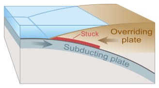
Tsunami can be generated when the sea floor abruptly deforms and vertically displaces the overlying water. Tectonic earthquakes are a particular kind of earthquake that are associated with the Earth's crustal deformation; when these earthquakes occur beneath the sea, the water above the deformed area is displaced from its equilibrium position. More specifically, a tsunami can be generated when thrust faults associated with convergent or destructive plate boundaries move abruptly, resulting in water displacement, owing to the vertical component of movement involved. Movement on normal (extensional) faults can also cause displacement of the seabed, but only the largest of such events (typically related to flexure in the outer trench swell) cause enough displacement to give rise to a significant tsunami, such as the 1977 Sumba and 1933 Sanriku events.-
-
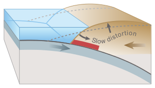 Overriding plate bulges under strain, causing tectonic uplift.
-
 Plate slips, causing subsidence and releasing energy into water.
-
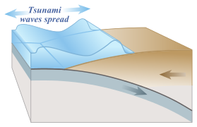 The energy released produces tsunami waves.


On April 1, 1946, a magnitude-7.8 (Richter Scale) earthquake occurred near the Aleutian Islands, Alaska. It generated a tsunami which inundated Hilo on the island of Hawai'i with a 14-metre high (46 ft) surge. The area where the earthquake occurred is where the Pacific Ocean floor is subducting (or being pushed downwards) under Alaska.
Examples of tsunami originating at locations away from convergent boundaries include Storegga about 8,000 years ago, Grand Banks 1929, Papua New Guinea 1998 (Tappin, 2001). The Grand Banks and Papua New Guinea tsunamis came from earthquakes which destabilised sediments, causing them to flow into the ocean and generate a tsunami. They dissipated before travelling transoceanic distances.
The cause of the Storegga sediment failure is unknown. Possibilities include an overloading of the sediments, an earthquake or a release of gas hydrates (methane etc.).
The 1960 Valdivia earthquake (Mw 9.5), 1964 Alaska earthquake (Mw 9.2), 2004 Indian Ocean earthquake (Mw 9.2), and 2011 Tōhoku earthquake (Mw9.0) are recent examples of powerful megathrust earthquakes that generated tsunamis (known as teletsunamis) that can cross entire oceans. Smaller (Mw 4.2) earthquakes in Japan can trigger tsunamis (called local and regional tsunamis) that can only devastate nearby coasts, but can do so in only a few minutes.
Landslides
In the 1950s, it was discovered that larger tsunamis than had previously been believed possible could be caused by giant submarine landslides. These rapidly displace large water volumes, as energy transfers to the water at a rate faster than the water can absorb. Their existence was confirmed in 1958, when a giant landslide in Lituya Bay, Alaska, caused the highest wave ever recorded, which had a height of 524 metres (over 1700 feet). The wave did not travel far, as it struck land almost immediately. Two people fishing in the bay were killed, but another boat managed to ride the wave.Another landslide-tsunami event occurred in 1963 when a massive landslide from Monte Toc entered the Vajont Dam in Italy. The resulting wave surged over the 262 m (860 ft) high dam by 250 metres (820 ft) and destroyed several towns. Around 2,000 people died Scientists named these waves megatsunamis.
Some geologists claim that large landslides from volcanic islands, e.g. Cumbre Vieja on La Palma in the Canary Islands, may be able to generate megatsunamis that can cross oceans, but this is disputed by many others.
In general, landslides generate displacements mainly in the shallower parts of the coastline, and there is conjecture about the nature of large landslides that enter water. This has been shown to lead to effect water in enclosed bays and lakes, but a landslide large enough to cause a transoceanic tsunami has not occurred within recorded history. Susceptible locations are believed to be the Big Island of Hawaii, Fogo in the Cape Verde Islands, La Reunion in the Indian Ocean, and Cumbre Vieja on the island of La Palma in the Canary Islands; along with other volcanic ocean islands. This is because large masses of relatively unconsolidated volcanic material occurs on the flanks and in some cases detachment planes are believed to be developing. However, there is growing controversy about how dangerous these slopes actually are.
Meteotsunamis
Some meteorological conditions, especially rapid changes in barometric pressure, as seen with the passing of a front, can displace bodies of water enough to cause trains of waves with wavelengths comparable to seismic tsunami, but usually with lower energies. These are essentially dynamically equivalent to seismic tsunami, the only differences being that meteotsunami lack the transoceanic reach of significant seismic tsunami, and that the force that displaces the water is sustained over some length of time such that meteotsunami can't be modelled as having been caused instantaneously. In spite of their lower energies, on shorelines where they can be amplified by resonance they are sometimes powerful enough to cause localised damage and potential for loss of life. They have been documented in many places, including the Great Lakes, the Aegean Sea, the English Channel, and the Balearic Islands, where they are common enough to have a local name, rissaga. In Sicily they are called marubbio and in Nagasaki Bay they are called abiki. Some examples of destructive meteotsunami include 31 March 1979 at Nagasaki and 15 June 2006 at Menorca, the latter causing damage in the tens of millions of euros.Meteotsunami should not be confused with storm surges, which are local increases in sea level associated with the low barometric pressure of passing tropical cyclones, nor should they be confused with setup, the temporary local raising of sea level caused by strong on-shore winds. Storm surges and setup are also dangerous causes of coastal flooding in severe weather but their dynamics are completely unrelated to tsunami waves.They are unable to propagate beyond their sources, as waves do.
Man-made or triggered tsunamis
See also: Tsunami bomb
There have been studies of the potential of induction of and at least one actual attempt to create tsunami waves as a tectonic weapon.In World War II, the New Zealand Military Forces initiated Project Seal, which attempted to create small tsunamis with explosives in the area of today's Shakespear Regional Park; the attempt failed.
There has been considerable speculation on the possibility of using nuclear weapons to cause tsunamis near to an enemy coastline. Even during World War II consideration of the idea using conventional explosives was explored. Nuclear testing in the Pacific Proving Ground by the United States seemed to generate poor results. Operation Crossroads fired two 20 kilotonnes of TNT (84 TJ) bombs, one in the air and one underwater, above and below the shallow (50 m (160 ft)) waters of the Bikini Atoll lagoon. Fired about 6 km (3.7 mi) from the nearest island, the waves there were no higher than 3–4 m (9.8–13.1 ft) upon reaching the shoreline. Other underwater tests, mainly Hardtack I/Wahoo (deep water) and Hardtack I/Umbrella (shallow water) confirmed the results. Analysis of the effects of shallow and deep underwater explosions indicate that the energy of the explosions doesn't easily generate the kind of deep, all-ocean waveforms which are tsunamis; most of the energy creates steam, causes vertical fountains above the water, and creates compressional waveforms. Tsunamis are hallmarked by permanent large vertical displacements of very large volumes of water which don't occur in explosions.
Characteristics

When the wave enters shallow water, it slows down and its amplitude (height) increases.

The wave further slows and amplifies as it hits land. Only the largest waves crest.
While everyday wind waves have a wavelength (from crest to crest) of about 100 metres (330 ft) and a height of roughly 2 metres (6.6 ft), a tsunami in the deep ocean has a much larger wavelength of up to 200 kilometres (120 mi). Such a wave travels at well over 800 kilometres per hour (500 mph), but owing to the enormous wavelength the wave oscillation at any given point takes 20 or 30 minutes to complete a cycle and has an amplitude of only about 1 metre (3.3 ft). This makes tsunamis difficult to detect over deep water, where ships are unable to feel their passage.
The velocity of a tsunami can be calculated by obtaining the square root of the depth of the water in metres multiplied by the acceleration due to gravity (approximated to 10 m sec2). For example, if the Pacific Ocean is considered to have a depth of 5000 metres, the velocity of a tsunami would be the square root of √5000 x 10 = √50000 = ~224 metres per second (735 feet per second), which equates to a speed of ~806 kilometres per hour or about 500 miles per hour. This formula is the same as used for calculating the velocity of shallow waves, because a tsunami behaves like a shallow wave as it peak to peak value reaches from the floor of the ocean to the surface.
The reason for the Japanese name "harbour wave" is that sometimes a village's fishermen would sail out, and encounter no unusual waves while out at sea fishing, and come back to land to find their village devastated by a huge wave.
As the tsunami approaches the coast and the waters become shallow, wave shoaling compresses the wave and its speed decreases below 80 kilometres per hour (50 mph). Its wavelength diminishes to less than 20 kilometres (12 mi) and its amplitude grows enormously. Since the wave still has the same very long period, the tsunami may take minutes to reach full height. Except for the very largest tsunamis, the approaching wave does not break, but rather appears like a fast-moving tidal bore. Open bays and coastlines adjacent to very deep water may shape the tsunami further into a step-like wave with a steep-breaking front.
When the tsunami's wave peak reaches the shore, the resulting temporary rise in sea level is termed run up. Run up is measured in metres above a reference sea level. A large tsunami may feature multiple waves arriving over a period of hours, with significant time between the wave crests. The first wave to reach the shore may not have the highest run up.
About 80% of tsunamis occur in the Pacific Ocean, but they are possible wherever there are large bodies of water, including lakes. They are caused by earthquakes, landslides, volcanic explosions, glacier calvings, and bolides.
Drawback

An illustration of the rhythmic "drawback" of surface water associated
with a wave. It follows that a very large drawback may herald the
arrival of a very large wave.
A typical wave period for a damaging tsunami is about 12 minutes. This means that if the drawback phase is the first part of the wave to arrive, the sea will recede, with areas well below sea level exposed after 3 minutes. During the next 6 minutes the tsunami wave trough builds into a ridge, and during this time the sea is filled in and destruction occurs on land. During the next 6 minutes, the tsunami wave changes from a ridge to a trough, causing flood waters to drain and drawback to occur again. This may sweep victims and debris some distance from land. The process repeats as the next wave arrives.
Scales of intensity and magnitude
As with earthquakes, several attempts have been made to set up scales of tsunami intensity or magnitude to allow comparison between different events.Intensity scales
The first scales used routinely to measure the intensity of tsunami were the Sieberg-Ambraseys scale, used in the Mediterranean Sea and the Imamura-Iida intensity scale, used in the Pacific Ocean. The latter scale was modified by Soloviev, who calculated the Tsunami intensity I according to the formula
 is the average wave height along the nearest coast. This scale, known as the Soloviev-Imamura tsunami intensity scale, is used in the global tsunami catalogues compiled by the NGDC/NOAA and the Novosibirsk Tsunami Laboratory as the main parameter for the size of the tsunami.
In 2013, following the intensively studied tsunamis in 2004 and 2011, a new 12 point scale was proposed, the Integrated Tsunami Intensity Scale (ITIS-2012), intended to match as closely as possible to the modified ESI2007 and EMS earthquake intensity scales.
Magnitude scales
The first scale that genuinely calculated a magnitude for a tsunami, rather than an intensity at a particular location was the ML scale proposed by Murty & Loomis based on the potential energy.Difficulties in calculating the potential energy of the tsunami mean that this scale is rarely used. Abe introduced the tsunami magnitude scale , calculated from,
Warnings and predictions
See also: Tsunami warning system

Tsunami warning sign
In the 2004 Indian Ocean tsunami drawback was not reported on the African coast or any other east-facing coasts that it reached. This was because the wave moved downwards on the eastern side of the fault line and upwards on the western side. The western pulse hit coastal Africa and other western areas.
A tsunami cannot be precisely predicted, even if the magnitude and location of an earthquake is known. Geologists, oceanographers, and seismologists analyse each earthquake and based on many factors may or may not issue a tsunami warning. However, there are some warning signs of an impending tsunami, and automated systems can provide warnings immediately after an earthquake in time to save lives. One of the most successful systems uses bottom pressure sensors, attached to buoys, which constantly monitor the pressure of the overlying water column.
Regions with a high tsunami risk typically use tsunami warning systems to warn the population before the wave reaches land. On the west coast of the United States, which is prone to Pacific Ocean tsunami, warning signs indicate evacuation routes. In Japan, the community is well-educated about earthquakes and tsunamis, and along the Japanese shorelines the tsunami warning signs are reminders of the natural hazards together with a network of warning sirens, typically at the top of the cliff of surroundings hills.
The Pacific Tsunami Warning System is based in Honolulu, Hawaiʻi. It monitors Pacific Ocean seismic activity. A sufficiently large earthquake magnitude and other information triggers a tsunami warning. While the subduction zones around the Pacific are seismically active, not all earthquakes generate tsunami. Computers assist in analysing the tsunami risk of every earthquake that occurs in the Pacific Ocean and the adjoining land masses.
As a direct result of the Indian Ocean tsunami, a re-appraisal of the tsunami threat for all coastal areas is being undertaken by national governments and the United Nations Disaster Mitigation Committee. A tsunami warning system is being installed in the Indian Ocean.

Some zoologists hypothesise that some animal species have an ability to sense subsonic Rayleigh waves from an earthquake or a tsunami. If correct, monitoring their behaviour could provide advance warning of earthquakes, tsunami etc. However, the evidence is controversial and is not widely accepted. There are unsubstantiated claims about the Lisbon quake that some animals escaped to higher ground, while many other animals in the same areas drowned. The phenomenon was also noted by media sources in Sri Lanka in the 2004 Indian Ocean earthquake. It is possible that certain animals (e.g., elephants) may have heard the sounds of the tsunami as it approached the coast. The elephants' reaction was to move away from the approaching noise. By contrast, some humans went to the shore to investigate and many drowned as a result.
Along the United States west coast, in addition to sirens, warnings are sent on television and radio via the National Weather Service, using the Emergency Alert System.
Forecast of tsunami attack probability
Kunihiko Shimazaki (University of Tokyo), a member of Earthquake Research committee of The Headquarters for Earthquake Research Promotion of Japanese government, mentioned the plan to public announcement of tsunami attack probability forecast at Japan National Press Club on 12 May 2011. The forecast includes tsunami height, attack area and occurrence probability within 100 years ahead. The forecast would integrate the scientific knowledge of recent interdisciplinarity and aftermath of the 2011 Tōhoku earthquake and tsunami. As the plan, announcement will be available from 2014.Mitigation
See also: Tsunami barrier

Japan, where tsunami science and response measures first began following a disaster in 1896, has produced ever-more elaborate countermeasures and response plans. The country has built many tsunami walls of up to 12 metres (39 ft) high to protect populated coastal areas. Other localities have built floodgates of up to 15.5 metres (51 ft) high and channels to redirect the water from incoming tsunami. However, their effectiveness has been questioned, as tsunami often overtop the barriers.
The Fukushima Daiichi nuclear disaster was directly triggered by the 2011 Tōhoku earthquake and tsunami, when waves exceeded the height of the plant's sea wall. Iwate Prefecture, which is an area at high risk from tsunami, had tsunami barriers walls totalling 25 kilometres (16 mi) long at coastal towns. The 2011 tsunami toppled more than 50% of the walls and caused catastrophic damage.
The Okushiri, Hokkaidō tsunami which struck Okushiri Island of Hokkaidō within two to five minutes of the earthquake on July 12, 1993 created waves as much as 30 metres (100 ft) tall—as high as a 10-story building. The port town of Aonae was completely surrounded by a tsunami wall, but the waves washed right over the wall and destroyed all the wood-framed structures in the area. The wall may have succeeded in slowing down and moderating the height of the tsunami, but it did not prevent major destruction and loss of life.
Waves and shallow water
When waves travel into areas of shallow water, they begin to be affected by the ocean bottom. The free orbital motion of the water is disrupted, and water particles in orbital motion no longer return to their original position. As the water becomes shallower, the swell becomes higher and steeper, ultimately assuming the familiar sharp-crested wave shape. After the wave breaks, it becomes a wave of translation and erosion of the ocean bottom intensifies
In fluid dynamics, the Boussinesq approximation for water waves is an approximation valid for weakly non-linear and fairly long waves. The approximation is named after Joseph Boussinesq, who first derived them in response to the observation by John Scott Russell of the wave of translation (also known as solitary wave or soliton). The 1872 paper of Boussinesq introduces the equations now known as the Boussinesq equations.
The Boussinesq approximation for water waves takes into account the vertical structure of the horizontal and vertical flow velocity. This results in non-linear partial differential equations, called Boussinesq-type equations, which incorporate frequency dispersion (as opposite to the shallow water equations, which are not frequency-dispersive). In coastal engineering, Boussinesq-type equations are frequently used in computer models for the simulation of water waves in shallow seas and harbours.
While the Boussinesq approximation is applicable to fairly long waves – that is, when the wavelength is large compared to the water depth – the Stokes expansion is more appropriate for short waves (when the wavelength is of the same order as the water depth, or shorter).


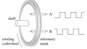
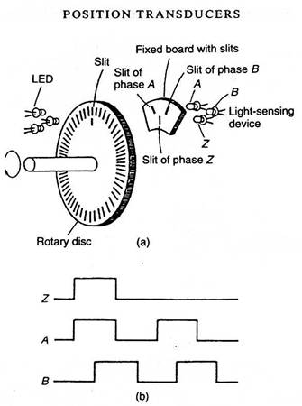
 Gambar 1. Blok penyusun rotary encoder
 (1)
(1) Gambar 2. Rangkaian tipikal penghasil pulsa pada rotary encoder
 Gambar 4. Contoh piringan dengan 10 cincin dan 10 LED – photo-transistor untuk membentuk sistem biner 10 bit.


 menggunakan frequencymeter dan periodimeter.
 (2)
(2) (3)
(3)


 Gambar 11. Pengukuran kecepatan dengan menggunakan Periodimeter