A Theoristic have got a Value fact + Virtual = Ideal Value .
A Practical have not got constant value and then changing is a true .
The track of ideal value always to everything moving so do the track of practical always
spring and random .
AMNIMARJEESLOW in PASCAL go to track up schrodinge spring on through the walls

( Gen. Mac Tech Zone MARIA PREFER to delta , derivative , integral , determinant BASIC )
Matrixs and determinants are often useful not just to apply them directly to but understand and solve other more complicated problems.
Many
problems in engineering can be described with systems of linear
equations. This is generally good since you can easily determine whether
it is solveable and then how to solve it. You can use determinants and
with that Cramer’s rule to solve it, even though the algorithm of Gauß
or iterative approaches might be more suited for larger problems. As you
can see it above you can use it to describe electronic circuits with
Kirchhoff laws.
Another problem are Eigenvalues and Eigenvector problems. To get a eigenvalue of a matrix you need to solve


. With the matrix and it’s Eigenvalues you can get the eigenvectors for
that matrix. This is important for the stability of systems. As you can
see above it can be used to explore buckling of sticks or the natural
frequency of damping systems.
Not
all systems can be described with normal functions. Some phenomenas
like a circuit with capacitors above need differential equations to be
described well.
If
your differential equation is not of first order, it has multiple
solutions that are a base of a vector space. To see whether your found
solutions all linear independent you take all solutions and its
derivation till the
th derivation of each solution so that you have a
Matrix. You can then take the determinant, the so called Wronskian
determinant. If it’s not zero for some x of your intervall, the
solutions are linear independent.
If
you not only have one differential equation but multiple you can solve
it again with the Eigenvalues and Eigenvectors of the Matrix or use
Putzer’s algorithm, if you have multiples times the same Eigenvalue.
If
you have a multidimensional integral and want to e.g. calculate the
electric charge from a(not constant) charge density, you will need to
integrate it. This often isn’t that easy in cartesian coordinates.
Better use a polar coordinate system for spheres or cylinder to have it
easier. This is a substitution for multidimensional integrals and like
you need for 1 dimension the derivate of your substitution, you need to
derivation in multiple dimensions. This is the Jacobian matrix and it’s
determinant since your small volume parts aren’t the same as before the
substitution.
In general, you have to know that not every thing in your mathematics course has directly an application.
-------------------------------------------------------------------------------------------------------------------------
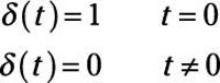
The delta function is a mathematical construct, not a real world signal. Signals in the real world that act as delta functions will always have a finite duration and amplitude. Just as in the discrete case, the continuous delta function is given the mathematical symbol: δ( ).
The delta function is a generalized function that can be defined as the limit of a class of delta sequences. The delta function is sometimes called "Dirac's delta function" or the "impulse symbol" (Bracewell 1999). ... The action of on , commonly denoted or , then gives the value at 0 of for any function .
A river delta is a landform created by deposition of sediment that is carried by a river as the flow leaves its mouth and enters slower-moving or stagnant water. This occurs where a river enters an ocean, sea, estuary, lake, reservoir, or (more rarely) another river that cannot carry away the supplied sediment.
Apply the Impulse Function to Circuit Analysis
The impulse function, also known as a Dirac delta function, helps you
measure a spike that occurs in one instant of time. Think of the spiked
impulse function (Dirac delta function) as one that’s infinitely large
in magnitude and infinitely thin in time, having a total area of 1.
Impulse forces occur for a short period of time, and the impulse
function allows you to measure them.
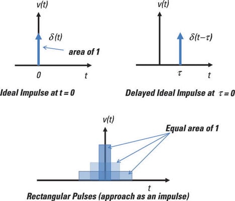
Visualize the impulse as a limiting form of a rectangular pulse of unit
area. Specifically, as you decrease the duration of the pulse, its
amplitude increases so that the area remains constant at unity. The more
you decrease the duration, the closer the rectangular pulse comes to
the impulse function.

The bottom diagram here shows the limiting form of the rectangular pulse approaching an impulse.
So what’s the practical use of the impulse function? By using the
impulse as an input signal to a system, you can reveal the output
behavior or character of a system. After you know the behavior of the
system for an impulse, you can describe the system’s output behavior for
any input.
Why is that? Because any input is modeled as a series of impulses
shifted in time with varying heights, amplitudes, or strengths.
Here’s the fancy pants description of the impulse function:
Another example of a real-world impulse function is a bomb. A powerful bomb has lots of energy occurring in a short amount of time. Similarly, fireworks, including cherry bombs, produce loud noises — audio energy — that occur as a series of popping noises having short durations.
Here’s the fancy pants description of the impulse function:
Identify impulse functions in the day-to-day
Some physical phenomena come very close to
being modeled with impulse functions. One example is lightning.
Lightning has lots of energy and occurs in a short amount of time. That
fits the description of an impulse function.
An ideal impulse has an infinitely high amplitude (high energy) and
is infinitely thin in time. As you drive through a lightning storm, you
may hear a popping noise if you’re tuned in to a radio weather station.
This noise occurs when the energy of the lightning interferes with the
signal coming from the radio weather station.Another example of a real-world impulse function is a bomb. A powerful bomb has lots of energy occurring in a short amount of time. Similarly, fireworks, including cherry bombs, produce loud noises — audio energy — that occur as a series of popping noises having short durations.
This mathematical description says that the impulse function occurs
at only one point in time; the function is zero elsewhere. The impulse
here occurs at the origin of time — that is, when you decide to let t = 0 (not at the beginning of the universe or anything like that).
The top-left diagram here shows an ideal unit impulse function having a large amplitude with a short duration.

You can describe the area of the impulse function as the strength of the impulse:
The top-left diagram here shows an ideal unit impulse function having a large amplitude with a short duration.
You can describe the area of the impulse function as the strength of the impulse:
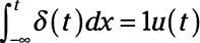
At time t = 0, the area is a constant having a value of 1; and before t = 0, the area is equal to 0. The integration of the impulse results in another funky function, u(t), called a step function. You can view the impulse as a derivative of the step function u(t) with respect to time:
What these two equations tell you is that if you know one function, you can determine the other function.
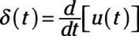
The area under the curve is given by strength K. The result of integrating the impulse leads you to another step function with amplitude or strength K.
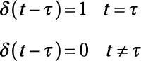
This equation says the impulse occurs only at a time later τ and nowhere else, or it’s equal to 0 at time not equal to τ. You see a delayed impulse in the top-right diagram shown here.
For a numerical example, let an impulse having a strength of 10 occur at delayed time τ = 5. You can describe the delayed impulse as
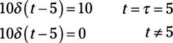
The equation says that the impulse, which has strength K = 10, occurs only at a time τ = 5 later and that the impulse occurs nowhere else. In other words, the impulse is equal to 0 when time is not equal to 5.
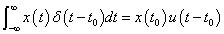
You do this evaluation only where the impulse occurs — at only one point and nowhere else. The preceding equation sifts out or selects the value of x(t) at time equal to t0. This integration is one of the easiest integrations you’ll encounter.
Here’s a simple numerical example with x(t) = 5t2 + 3t + 6 and t0 = 5:
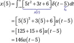
Pretty funky way to integrate analytically, huh? The integration leads to a delayed (or time-shifted) step function (or constant) starting at a delayed time of t0 = 5.
What these two equations tell you is that if you know one function, you can determine the other function.
Change the strength of the impulse
The figure shows an impulse with an area (or strength) equal to 1. To have a different area or strength K, you can modify the impulse:The area under the curve is given by strength K. The result of integrating the impulse leads you to another step function with amplitude or strength K.
Delay an impulse
Impulses can be delayed. Analytically, you can describe a delayed impulse that occurs later, say, at time τ:This equation says the impulse occurs only at a time later τ and nowhere else, or it’s equal to 0 at time not equal to τ. You see a delayed impulse in the top-right diagram shown here.
For a numerical example, let an impulse having a strength of 10 occur at delayed time τ = 5. You can describe the delayed impulse as
The equation says that the impulse, which has strength K = 10, occurs only at a time τ = 5 later and that the impulse occurs nowhere else. In other words, the impulse is equal to 0 when time is not equal to 5.
Evaluate impulse functions with integrals
Assuming x(t) is a continuous function that’s multiplied by a time-shifted (or delayed) impulse, the integral of the product is expressed and evaluated as follows:You do this evaluation only where the impulse occurs — at only one point and nowhere else. The preceding equation sifts out or selects the value of x(t) at time equal to t0. This integration is one of the easiest integrations you’ll encounter.
Here’s a simple numerical example with x(t) = 5t2 + 3t + 6 and t0 = 5:
Pretty funky way to integrate analytically, huh? The integration leads to a delayed (or time-shifted) step function (or constant) starting at a delayed time of t0 = 5.
You can model any smooth function x(t) as a series of delayed and time-shifted impulses in the following way:
This equation says you can break up any function x(t) into a sum of a whole bunch of delayed impulse functions with different strengths. The value of the strength is simply the function x(t) evaluated where the shifted impulse occurs at time τ or t.
------------------------------------------------------------------------------------------------------------------------
Algebra and Geometry in Electronics
Magnetic field near a bar magnet
 Consider the bar magnet shown. The
magnetic field strength H at a test point P
along the axis of the magnet is given by the formula:
Consider the bar magnet shown. The
magnetic field strength H at a test point P
along the axis of the magnet is given by the formula:Problem:
Show that at large distances H falls off as the inverse cube of the distance.Solution
The phrase "at large distances" means that the distance d becomes very large; much larger than the distance L. If we let d become very large in the original expression:
H = + 0 - 0
since d is in the denominator. This is of no help. What is
required is to combine the two fractions into one. Start by
putting them over a common denominator, like this:
Electronics:
Linear Algebra
One of the most important applications of linear algebra to electronics is to analyze electronic circuits that cannot be described using the rules for resistors in series or parallel such as the one shown to the right. The goal is to calculate the current flowing in each branch of the circuit or to calculate the voltage at each node of the circuit.
Knowing the branch currents, the nodal voltages can easily be calculated, and knowing the nodal voltages, the branch currents can easily be calculated. Loop analysis finds the currents directly and nodal analysis find the voltages directly. Which method is simpler depends on the given circuit. Nodal analysis is important because its answers can be directly compared with voltage measurements taken in a circuit, whereas currents are not so easily measured in a circuit (one must cut wires)
Electronics and Trignometry
Background
Alternating current (AC) is current which flows back and forth along a conductor. (In contrast, direct current (DC) is current which flows in one direction only.) Alternating current is the result of an alternating voltage (force) pushing electric charges back and forth.The diagram to the right shows an AC generator capable of producing an alternating voltage. It is basically a loop of wire rotating between the poles of a magnet. The diagram also shows a graph of the voltage v produced by the generator as a function of time t as the loop L rotates through one complete circle .
Electronics: RC circuits and Exponential Charging
 An RC circuit is one that contains a resistor and capacitor.
Consider the RC circuit shown in the figure. Suppose that the
switch is closed at time t = 0 s and
that the capacitor has no initial stored charge on it. Once the
switch closes, a current will begin flowing in the circuit.
This current will deposit charge on the capacitor, leading to a
voltage vC(t) across
the capacitor.
An RC circuit is one that contains a resistor and capacitor.
Consider the RC circuit shown in the figure. Suppose that the
switch is closed at time t = 0 s and
that the capacitor has no initial stored charge on it. Once the
switch closes, a current will begin flowing in the circuit.
This current will deposit charge on the capacitor, leading to a
voltage vC(t) across
the capacitor.The current i(t) is given by the formula:
Electronics: Using Derivatives with Circuits
The 4 concepts of calculus?
With just four main ideas on which to focus, students will find calculus more manageable, and they'll have an easier time understanding, connecting, and remembering important concepts. Each concept is clearly developed through graphical, algebraic, numerical, and verbal methods, so differentiation is made easy.
Waveform Differentiation
A waveform is a function that repeats itself or cycles after a specified period of time. This time, denoted T, is called the period of the waveform. The diagram to the right shows an electronic circuit that takes
as input a voltage waveform and gives as output an approximation
of the derivative of that waveform. The approximation can be made
quite good by using small enough values of R and
C or restricting ourselves to slowly varying input
voltages.
The diagram to the right shows an electronic circuit that takes
as input a voltage waveform and gives as output an approximation
of the derivative of that waveform. The approximation can be made
quite good by using small enough values of R and
C or restricting ourselves to slowly varying input
voltages.To calculate the derivative of a waveform it is sufficient to calculate the derivative of just the first cycle. This is because the derivative of a waveform is another waveform. The derivative of all the other cycles will look the same as that of the first cycle. If f (t) is the formula for the first cycle then f ′ (t), its derivative, is the formula for the derivative of the first cycle. If required, the formula for the derivative of any other cycle can be found by simply applying a shift to the formula for the derivative of the first cycle.
Electronics: Integrals and RMS Signals
The average or mean of a set of numbers is found by adding up
the numbers and dividing by the number of numbers. The
mean value of a function is the generalization
of this idea. The mean value of any function
f(x) is defined as the mean height of the
function. It can be found by calculating the area under the
function and dividing by the width of the function. We will
denote the mean value of a function f using angle
brackets like this:
 Then using calculus notation the above statement can be
written as:
Then using calculus notation the above statement can be
written as:
 (We are assuming that the function runs from a to
b, so integrating from a to b gives
the area under the function and dividing by b - a
divides by the width of the function.)
(We are assuming that the function runs from a to
b, so integrating from a to b gives
the area under the function and dividing by b - a
divides by the width of the function.)
If the function is periodic (i.e. if the function repeats itself exactly after a certain amount of time, called the period, T) then we can replace the above formula by this formula:
 In other words we only have to find the area for one cycle and
divide by the width of one cycle.
In other words we only have to find the area for one cycle and
divide by the width of one cycle.
The RMS value of a function is related to the idea of the standard deviation of a set of numbers. The RMS value of a function is defined as the square root of the mean value of the square of a function. In other words to get the RMS value of a function we follow these three steps:
 Then using calculus notation the above procedure can be
written as:
Then using calculus notation the above procedure can be
written as:
 (Again we are assuming that the function runs from a
to b, so integrating from a to b gives
the area under the squared function and dividing by b -
a gives the mean of the squared function.)
(Again we are assuming that the function runs from a
to b, so integrating from a to b gives
the area under the squared function and dividing by b -
a gives the mean of the squared function.)
If the function is periodic with period T then we can replace the above formula by this formula:
Electronics:
 Put the above equation in differential form.
 Integrate both sides of the equation.
 Solve for the current i. First isolate the logarithm.
 Express in exponential form.
 Substitute the initial conditions into this equation to
evaluate the constant A. The initial conditions are i=0 at
t=0.
Substitute the initial conditions into this equation to
evaluate the constant A. The initial conditions are i=0 at
t=0.
 Thus the equation becomes
 Evaluate the expression for the values given in the circuit
diagram.
Evaluate the expression for the values given in the circuit
diagram.
 A graph of this function is shown below. Note that if the
inductor were absent the current would rise
instantly to 5 amperes, the value given by ohms
law, i=E/R. The presence of the inductor causes the current to
rise exponentially to 5 amperes, with the
characteristic time being 1/2000 s.
A graph of this function is shown below. Note that if the
inductor were absent the current would rise
instantly to 5 amperes, the value given by ohms
law, i=E/R. The presence of the inductor causes the current to
rise exponentially to 5 amperes, with the
characteristic time being 1/2000 s.
If the function is periodic (i.e. if the function repeats itself exactly after a certain amount of time, called the period, T) then we can replace the above formula by this formula:
The RMS value of a function is related to the idea of the standard deviation of a set of numbers. The RMS value of a function is defined as the square root of the mean value of the square of a function. In other words to get the RMS value of a function we follow these three steps:
- Square the function (i.e. draw a new function whose height everywhere is the square of the original function),
- calculate the Mean of this new function (This can be done using the above formula, namely, finding the area under the new function, and dividing by the width of the function),
- taking the square Root
(Again we are assuming that the function runs from a
to b, so integrating from a to b gives
the area under the squared function and dividing by b -
a gives the mean of the squared function.)If the function is periodic with period T then we can replace the above formula by this formula:
Electronics:
Circuit Analysis Using Differential Equations
Problem:
Find the current in the circuit to the right after time t=0. The switch is closed at t=0, and the initial current in the circuit is zero.Solution:
Using Kirchoff’s Voltage Law:
vL + vR = E
Express the voltage equation in terms of current.
L di = (E-Ri) dt
Separate the variables.
Solve for the current i. First isolate the logarithm.
Substitute the initial conditions into this equation to
evaluate the constant A. The initial conditions are i=0 at
t=0.
Thus the equation becomes
Evaluate the expression for the values given in the circuit
diagram.
Robotics:Robotic Arm Coordinates and Geometry
The diagram shows a robot with a telescoping arm.
Note the two basic variables:
θ= angular inclination of the arm (rads)
R = length of the arm (meters)
Each of these variables can be controlled separately.
In any practical situation, the manipulator (the component at the end of the arm) has to move in a prescribed way. Suppose that the angle θ can be increased or decreased, in response to commands from a computer. While this is happening, the arm can also be extended or retracted. We want to obtain a mathematical description of how R should be adjusted, in relation to θ, so that the manipulator will trace out a particular path.
(Note that the control of an actual robot is a much more complicated affair. For example, movements have to be graduated, because of inertia, and in order to prevent excessive strain on mechanical linkages. Robots are programmed to move according to complex dynamical equations that take into account velocity, acceleration, and mass distributions.)
Robotics: Using Transformation Matrices to Change from One Coordinate System to Another in Robotics
Background
In many robotics problems it is useful to define more than one coordinate system. For example in the picture to the right we have defined three coordinate systems. We have attached a coordinate system called B to the robot’s base, another coordinate system called H to its hand and another called P to the piece that the robot must grasp. (By attached we mean that if we move the base, the hand or the piece then the corresponding coordinate system moves with it.) Coordinate system P is useful for locating points on the cylinder. Coordinate system B is useful for describing the location of the hand. And coordinate system H is useful for measuring distances from the hand.Often we know the position and orientation of the piece P relative to the robot’s base B but we need to know it relative to the hand H so that the hand can be moved correctly to pick up the piece. This can be computed if we know the position and orientation of the hand relative to the base. Note that orientation as well as position is important if we want the hand to be properly oriented to grasp the piece.
In this background section we will explain how a transformation matrix can be used to describe the location and orientation of a second coordinate system with respect to a first coordinate system.
Consider the following transformation matrix
T = 
Here is how this transformation matrix can be
used to describe the location and orientation of a second
coordinate system relative to a first coordinate system. We
apply the transformation matrix to the origin and the
endpoints of the unit vectors of the first coordinate
system. This matrix multiplication produces the origin and
the endpoints of the unit vectors of the second coordinate
system:
 These two coordinate systems are shown in the picture to
the right. (The second coordinate system is the one with
the tick marks.) Points can be located relative to either
coordinate system. For example the point P is
located at (x’ = 2, y’ =
1, z’ = 1) in the second coordinate system
and at (x = -5, y = 7,
z = 3) in
the first coordinate system.
These two coordinate systems are shown in the picture to
the right. (The second coordinate system is the one with
the tick marks.) Points can be located relative to either
coordinate system. For example the point P is
located at (x’ = 2, y’ =
1, z’ = 1) in the second coordinate system
and at (x = -5, y = 7,
z = 3) in
the first coordinate system.Probably the quickest way to "design" a transformation matrix like
T =
is to notice that the three columns of the 3x3
submatrix give the orientation of the second
coordinate system in terms of the first like this:
 and that the three element vector
Robotics: Linear Velocity of a Piston-Wheel System
 As the flywheel rotates at a constant rate of 500 rpm, the
piston moves back and forth along a horizontal line. If R = 10 cm
and L = 40 cm then what is the linear velocity of the piston,
when angle θ = 160°?
As the flywheel rotates at a constant rate of 500 rpm, the
piston moves back and forth along a horizontal line. If R = 10 cm
and L = 40 cm then what is the linear velocity of the piston,
when angle θ = 160°?Solution:
In the triangle with sides R and L, name the third side (the base) x.R and L are constant, but x is a function of time, x(t). The desired velocity is dx/dt.
Apply the Cosine Law:
L2 = R2 + x2 -
2 R x cos θ [equation 1]
Recalling that θ and therefore x are functions of time,
perform implicit differentiation:
0 = 2x dx/dt - 2R [ dx/dt cos θ- x sin (θ)
dθ/dt ] [equation 2]
To use this equation to find dx/dt, we need R, θ,
dθ/dt, and x.- R = 10
- θ= 160°, cos (θ)= -0.9397, sin (θ)= 0.3420
- dθ/dt = 500 rpm = (500)(2π)/60 rad/sec = 52.36 rad/sec
- To find x when R= 10 and L = 40 we must solve equation [1]:
402 = 102 + x2 - 2 (10) x (-.9397)This becomes
x2 + 18.79 x - 1500 = 0The roots are -49.25 and 30.46, and we need the positive root.
0 = 2(30.46) (dx/dt) - 2 (10) [ - .9397 dx/dt - 30.46 ( .3420)
(52.36)]
(-60.92 - 18.79) dx/dt = 10909
dx/dt = -136.9 cm/sec
The negative sign indicates that x is getting smaller, which
is correct when θ < 180°________________________________________________________________________________
ACTIVE AREA ON FUNCTION ELECTRONICS
A transistor is a semiconductor device used to amplify or switch electronic signals and electrical power. ... A voltage or current applied to one pair of the transistor's terminals controls the current through another pair of terminals.
An integrated circuit, or IC, is small chip that can function as an amplifier, oscillator, timer, microprocessor, or even computer memory. An IC is a small wafer, usually made of silicon, that can hold anywhere from hundreds to millions of transistors, resistors, and capacitors.
Impulse response
In signal processing, the impulse response, or impulse response function (IRF), of a dynamic system is its output when presented with a brief input signal, called an impulse. More generally, an impulse response is the reaction of any dynamic system in response to some external change. In both cases, the impulse response describes the reaction of the system as a function of time (or possibly as a function of some other independent variable that parameterizes the dynamic behavior of the system).In all these cases, the dynamic system and its impulse response may be actual physical objects, or may be mathematical systems of equations describing such objects.
Since the impulse function contains all frequencies, the impulse response defines the response of a linear time-invariant system for all frequencies.
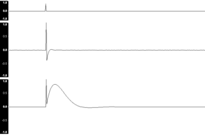
The Impulse response from a simple audio system. Showing, from top to bottom, the original impulse, the response after high frequency boosting, and the response after low frequency boosting.
Mathematical considerations
Mathematically, how the impulse is described depends on whether the system is modeled in discrete or continuous time. The impulse can be modeled as a Dirac delta function for continuous-time systems, or as the Kronecker delta for discrete-time systems. The Dirac delta represents the limiting case of a pulse made very short in time while maintaining its area or integral (thus giving an infinitely high peak). While this is impossible in any real system, it is a useful idealisation. In Fourier analysis theory, such an impulse comprises equal portions of all possible excitation frequencies, which makes it a convenient test probe.Any system in a large class known as linear, time-invariant (LTI) is completely characterized by its impulse response. That is, for any input, the output can be calculated in terms of the input and the impulse response. The impulse response of a linear transformation is the image of Dirac's delta function under the transformation, analogous to the fundamental solution of a partial differential operator.
It is usually easier to analyze systems using transfer functions as opposed to impulse responses. The transfer function is the Laplace transform of the impulse response. The Laplace transform of a system's output may be determined by the multiplication of the transfer function with the input's Laplace transform in the complex plane, also known as the frequency domain. An inverse Laplace transform of this result will yield the output in the time domain.
To determine an output directly in the time domain requires the convolution of the input with the impulse response. When the transfer function and the Laplace transform of the input are known, this convolution may be more complicated than the alternative of multiplying two functions in the frequency domain.
The impulse response, considered as a Green's function, can be thought of as an "influence function": how a point of input influences output.
Practical applications
In practical systems, it is not possible to produce a perfect impulse to serve as input for testing; therefore, a brief pulse is sometimes used as an approximation of an impulse. Provided that the pulse is short enough compared to the impulse response, the result will be close to the true, theoretical, impulse response. In many systems, however, driving with a very short strong pulse may drive the system into a nonlinear regime, so instead the system is driven with a pseudo-random sequence, and the impulse response is computed from the input and output signals.Loudspeakers
An application that demonstrates this idea was the development of impulse response loudspeaker testing in the 1970s. Loudspeakers suffer from phase inaccuracy, a defect unlike other measured properties such as frequency response. Phase inaccuracy is caused by (slightly) delayed frequencies/octaves that are mainly the result of passive cross overs (especially higher order filters) but are also caused by resonance, energy storage in the cone, the internal volume, or the enclosure panels vibrating. Measuring the impulse response, which is a direct plot of this "time-smearing," provided a tool for use in reducing resonances by the use of improved materials for cones and enclosures, as well as changes to the speaker crossover. The need to limit input amplitude to maintain the linearity of the system led to the use of inputs such as pseudo-random maximum length sequences, and to the use of computer processing to derive the impulse response.Electronic processing
Impulse response analysis is a major facet of radar, ultrasound imaging, and many areas of digital signal processing. An interesting example would be broadband internet connections. DSL/Broadband services use adaptive equalisation techniques to help compensate for signal distortion and interference introduced by the copper phone lines used to deliver the service.Control systems
In control theory the impulse response is the response of a system to a Dirac delta input. This proves useful in the analysis of dynamic systems; the Laplace transform of the delta function is 1, so the impulse response is equivalent to the inverse Laplace transform of the system's transfer function.Acoustic and audio applications
In acoustic and audio applications, impulse responses enable the acoustic characteristics of a location, such as a concert hall, to be captured. Various packages are available containing impulse responses from specific locations, ranging from small rooms to large concert halls. These impulse responses can then be utilized in convolution reverb applications to enable the acoustic characteristics of a particular location to be applied to target audio.
=======================================================================
Electronic Circuits - Signals
A Signal can be understood as "a representation that gives some information about the data present at the source from which it is produced." This is usually time varying. Hence, a signal can be a source of energy which transmits some information. This can easily be represented on a graph.
Examples
- An alarm gives a signal that it’s time.
- A cooker whistle confirms that the food is cooked.
- A red light signals some danger.
- A traffic signal indicates your move.
- A phone rings signaling a call for you.
Types of Signals
Signals can be classified either as Analog or Digital, depending upon their characteristics. Analog and Digital signals can be further classified, as shown in the following image.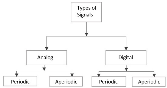
Analog Signal
A continuous time-varying signal, which represents a time-varying quantity, can be termed as an Analog Signal. This signal keeps on varying with respect to time, according to the instantaneous values of the quantity, which represents it.Digital Signal
A signal which is discrete in nature or which is non-continuous in form can be termed as a Digital signal. This signal has individual values, denoted separately, which are not based on previous values, as if they are derived at that particular instant of time.Periodic Signal & Aperiodic Signal
Any analog or digital signal, that repeats its pattern over a period of time, is called as a Periodic Signal. This signal has its pattern continued repeatedly and is easy to be assumed or to be calculated.Any analog or digital signal, that doesn’t repeat its pattern over a period of time, is called as Aperiodic Signal. This signal has its pattern continued but the pattern is not repeated and is not so easy to be assumed or to be calculated.
Signals & Notations
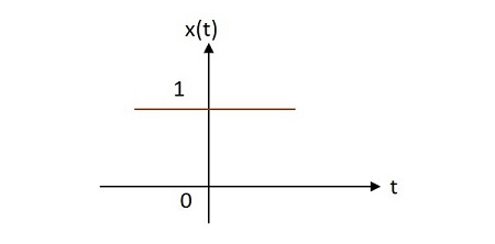
Among the Periodic Signals, the most commonly used signals are Sine wave, Cosine wave, Triangular waveform, Square wave, Rectangular wave, Saw-tooth waveform, Pulse waveform or pulse train etc. let us have a look at those waveforms.Unit Step Signal
The unit step signal has the value of one unit from its origin to one unit on the X-axis. This is mostly used as a test signal. The image of unit step signal is shown below.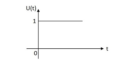 The unit step function is denoted by $u\left ( t \right )$. It is defined as −
$$u\left ( t \right )=\left\{\begin{matrix}1 & t\geq 0\\ 0 & t< 0\end{matrix}\right.$$
Unit Impulse Signal
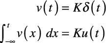
The unit impulse signal has the value of one unit at its origin. Its area is one unit. The image of unit impulse signal is shown below.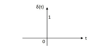 The unit impulse function is denoted by ẟ(t). It is defined as
$$\delta \left ( t \right )=\left\{\begin{matrix} \infty \:\:if \:\:t=0\\0 \:\:if \:\:t\neq 0\end{matrix}\right.$$
$$\int_{-\infty }^{\infty }\delta \left ( t \right )d\left ( t \right )=1$$
$$\int_{-\infty }^{t }\delta \left ( t \right )d\left ( t \right )=u\left ( t \right )$$
$$\delta \left ( t \right )=\frac{du\left ( t \right )}{d\left ( t \right )} $$
Unit Ramp Signal
The unit ramp signal has its value increasing exponentially from its origin. The image of unit ramp signal is shown below.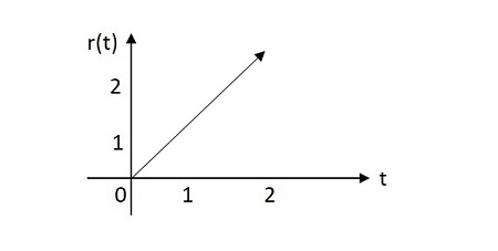 The unit ramp function is denoted by u(t). It is defined as −
$$\int_{0}^{t}u\left ( t \right ) d\left ( t \right )=\int_{0}^{t} 1 dt =t=r\left ( t \right )$$
$$u\left ( t \right )=\frac{dr\left ( t \right )}{dt}$$
Unit Parabolic Signal
The unit parabolic signal has its value altering like a parabola at its origin. The image of unit parabolic signal is shown below.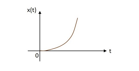 The unit parabolic function is denoted by $u\left ( t \right )$. It is defined as −
$$\int_{0}^{t}\int_{0}^{t}u\left ( t \right )dtdt=\int_{0}^{t}r\left ( t \right )dt=\int_{0}^{t} t.dt=\frac{t^{2}}{2}dt=x\left ( t \right )$$
$$r\left ( t \right )=\frac{dx\left ( t \right )}{dt}$$
$$u\left ( t \right )=\frac{d^{2}x\left ( t \right )}{dt^{2}}$$
Signum Function
The Signum function has its value equally distributed in both positive and negative planes from its origin. The image of Signum function is shown below.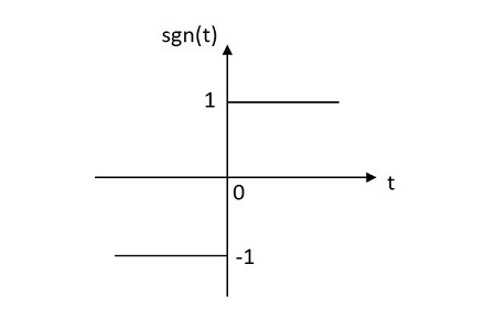 The Signum function is denoted by sgn(t). It is defined as
$$sgn\left ( t \right )=\left\{\begin{matrix} 1 \:\: for \:\: t\geq 0\\-1 \:\: for \:\:t < 0\end{matrix}\right.$$
$$sgn\left ( t \right )=2u\left ( t \right ) -1$$
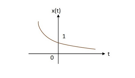
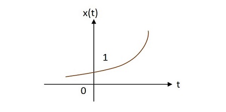
Exponential Signal
The exponential signal has its value varying exponentially from its origin. The exponential function is in the form of −$$x\left ( t \right ) =e^{\alpha t}$$
The shape of exponential can be defined by $\alpha$. This function can be understood in 3 cases
Case 1 −
If $\alpha = 0\rightarrow x\left ( t \right )=e^{0}=1$
 Case 2 −
If $\alpha <0$ then $x\left ( t \right )=e^{\alpha t}$ where $\alpha$ is negative. This shape is called as decaying exponential.
 Case 3 −
If $\alpha > 0$ then $x\left ( t \right )=e^{\alpha t}$ where $\alpha$ is positive. This shape is called as raising exponential.
Rectangular Signal
The rectangular signal has its value distributed in rectangular shape in both positive and negative planes from its origin. The image of rectangular signal is shown below.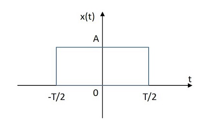 The rectangular function is denoted by $x\left ( t \right )$. It is defined as
 $$x\left ( t \right )=A \:rect\left [ \frac{t}{T} \right ]$$
Triangular Signal
The rectangular signal has its value distributed in triangular shape in both positive and negative planes from its origin. The image of triangular signal is shown below.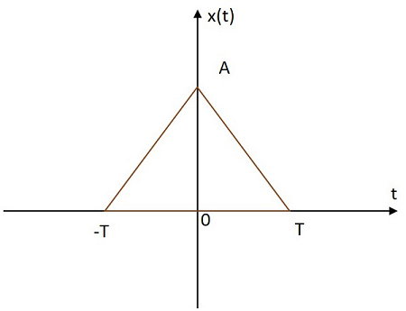 The triangular function is denoted by$x\left ( t \right )$. It is defined as
$$x\left ( t \right )=A \left [ 1-\frac{\left | t \right |}{T} \right ]$$
Sinusoidal Signal
The Sinusoidal signal has its value varying sinusoidally from its origin. The image of Sinusoidal signal is shown below.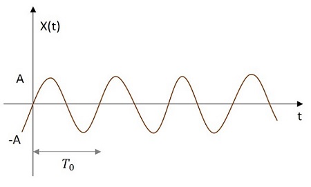 The sinusoidal function is denoted by x (t). It is defined as −
$$x\left ( t \right )=A \cos \left ( w_{0} t\pm \phi \right )$$
or
$$x\left ( t \right )=A sin\left ( w_{0}t\pm \phi \right )$$Where $T_{0}=\frac{2 \pi}{w_{0}}$
Sinc Function
The Sinc signal has its value varying according to a particular relation as in given equation below. It has its maximum value at the origin and goes on decreasing as it moves away. The image of a Sinc function signal is shown below.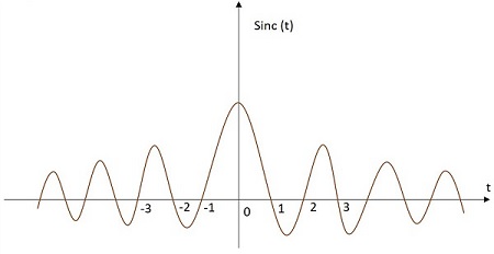 The Sinc function is denoted by sinc(t). It is defined as −
$$sinc\left ( t \right )=\frac{sin\left ( \pi t \right )}{\pi t}$$
So, these are the different signals we mostly come across in the field of Electronics and Communications. Every signal can be defined in a mathematical equation to make the signal analysis easier.
Each signal has a particular wave shape as mentioned before. The shaping of the wave may alter the content present in the signal. Anyways, it is the decision to be made by the design engineer whether to alter a wave or not for any particular circuit.
=======================================================================
Outer space in electronic networks for Electronic and Cyber Warfare in Outer Space
communication is used in space ? One of these forms is commonly called radio. The astronauts have devices in their helmets which transfer the sound waves from their voices into radio waves and transmit it to the ground (or other astronauts in space) .
At the International Space Station (ISS), astronauts make use of radio waves to access the internet since the atmosphere doesn't interfere with them. It's like how people use GPS technology. A signal is sent to a satellite, which then tracks the user's specific location and sends this information to the GPS receiver.
Electronics work in space ? So in a basic sense, not much really changes, and it's possible, with a bit of work, to use off-the-shelf components to do the same job out in space. However, there's a subtler way in which earth-bound electronics do benefit from Earth's magnetic field.
The Deep Space Network (DSN) consists of antenna complexes at three locations around the world, and forms the ground segment of the communications system for deep space missions. These facilities, approximately 120 longitude degrees apart on Earth, provide continuous coverage and tracking for deep space missions.
pictures sent from space?
phones work in space ? NASA Sends Cell Phones (Regular Old Cell Phones) Into Space. With just a touch of programming, NASA has turned some Nexus Ones into satellites .


Space industry is undergoing some profound changes, from the ... components and installing and connecting the electronics and other devices ..
Spacecraft equipment is a proven, trusted equipment supplier offering an extensive portfolio for space-related applications in telecommunications, Earth and space observation, ground and space navigation, science, launchers and manned space flight. With an unparalleled track record for in-orbit reliability, Airbus possesses all the expertise required to help design, engineer and implement disruptive new space missions.
communication is used in space ? One of these forms is commonly called radio. The astronauts have devices in their helmets which transfer the sound waves from their voices into radio waves and transmit it to the ground (or other astronauts in space) .
At the International Space Station (ISS), astronauts make use of radio waves to access the internet since the atmosphere doesn't interfere with them. It's like how people use GPS technology. A signal is sent to a satellite, which then tracks the user's specific location and sends this information to the GPS receiver.
Electronics work in space ? So in a basic sense, not much really changes, and it's possible, with a bit of work, to use off-the-shelf components to do the same job out in space. However, there's a subtler way in which earth-bound electronics do benefit from Earth's magnetic field.
The Deep Space Network (DSN) consists of antenna complexes at three locations around the world, and forms the ground segment of the communications system for deep space missions. These facilities, approximately 120 longitude degrees apart on Earth, provide continuous coverage and tracking for deep space missions.
pictures sent from space?
Spacecraft send information and pictures back to Earth using the Deep Space Network (DSN), a collection of big radio antennas. ... Spacecraft send information and pictures back to Earth using the Deep Space Network, or DSN. The DSN is a collection of big radio antennas in different parts of the world.
phones work in space ? NASA Sends Cell Phones (Regular Old Cell Phones) Into Space. With just a touch of programming, NASA has turned some Nexus Ones into satellites .
Space industry is undergoing some profound changes, from the ... components and installing and connecting the electronics and other devices ..
Spacecraft equipment
Spacecraft equipment is a proven, trusted equipment supplier offering an extensive portfolio for space-related applications in telecommunications, Earth and space observation, ground and space navigation, science, launchers and manned space flight. With an unparalleled track record for in-orbit reliability, Airbus possesses all the expertise required to help design, engineer and implement disruptive new space missions.
Avionics
an avionics product portfolio that covers a complete
range of compact and powerful onboard computers, new-generation GNSS
(Global Navigation Satellite System) receivers, launcher electronics and
other world-class platform data handling equipment and interface units .
Power
power solutions, has vast experience in providing turnkey solar arrays, photovoltaic assemblies and solar cell assemblies for institutional and commercial applications. The company also offers a full range of electronics – including power control units, power processing units for electric propulsion and electric power conditioners.
Payload Products
With more than two decades of experience and multiple innovations in navigation electronics and space-borne Mass Memories, mass data storage that provides high precision and innovative solutions for all types of missions. The company offers payload data handling units with compression and encryption features; radar and video electronic units; payload instrument control units; high precision, low noise timing solutions, for navigation constellations and scientific applications and more .
Pure line
All components are intensively radiation-tested to ensure flawless
in-orbit operation for years in low-Earth orbit. This new space product
line has now been extended to wider applications on satellites and
spacecraft .
Testing on high-end antenna measurement techniques :
----------------------------------------------------------------------------------------------------------------------------


Gen . Mac Tech Zone Function and NET
--------------------------------------------------------------------------------------------------------------------------
----------------------------------------------------------------------------------------------------------------------------
Gen . Mac Tech Zone Function and NET
--------------------------------------------------------------------------------------------------------------------------