


Blood is RED ?
Blood is red because it is made up of cells
that are red, which are called red blood cells. But, to understand why
these cells are red you have to study them on a molecular level. Within
the red blood cells there is a protein called hemoglobin. Each
hemoglobin protein is made up subunits called hemes, which are
what give blood its red color. More specifically, the hemes can bind
iron molecules, and these iron molecules bind oxygen. The blood cells
are red because of the interaction between iron and oxygen. (Even more
specifically, it looks red because of how the chemical bonds between the
iron and the oxygen reflect light.) And it's very important for blood
to be able to carry oxygen because when blood flows through the lungs,
the blood picks up oxygen, and the blood carries this oxygen to the rest
of the body until the oxygen is all used up -- the blood then returns
to the lungs to get more oxygen.
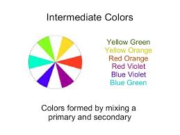
Magnetic and Electric Colours
In Colour Therapy, Red, Orange, and Yellow are referred
to as magnetic/warm colours - Blue, Indigo and Violet are referred to as
electric/cool colours.
Generally speaking, the three higher colours are calming,
and the three lower colours are stimulating and green is the balance
between the two types of energy.
Colours and Frequencies
In terms of Colour Therapy, the shortest wavelength
colours - are described as being cool electric colours
and the lowest wavelength colours - are described as being warm magnetic
colours.
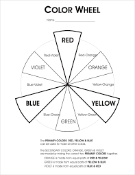
The diagram on the right, shows the seven rainbow colours in order of their frequency.
Violet is at the top of the column since it has the shortest wavelength and the highest frequency.
Red at the base with the longest wavelength and lowest frequency.
All seven colours of the spectrum can be seen by passing light through a prism. The three 'higher'
colours of - Violet, Indigo and Blue are in Colour Therapy Terms called the cool
/ electric colours and generally indicate calm/and coolness.
The three ' lower ' colours of Yellow, Orange and Red
are in Colour Therapy Terms called the warm / magnetic colours and
generally these are warming and activating colours. The colour Green is
the balance between the cool and warm rays.
 Similarity Matching vs. Thresholding
In reality you must calibrate your sensors before they will work. This means you must use your sensor(s)
to sense the object, record the readings, then make a chart using this data. That way when your robot is doing its thing
and senses the same object, it can compare the similarity of the new reading vs. the calibrating reading.
For example, suppose your robot needs to follow a white line on a grey floor. Your robot would use a
microcontroller to sense the analog value from the sensor.
During the calibration phase your robot measured an analog value of 95 for the grey floor, 112 for the white line,
and then stored these values in memory.
Now your robot is on the line, and a sensor reads 108. What does that mean? Is it on the line or not?
Using the
thresholding method, you add both calibrated numbers and divide by two to find the average middle number.
For example, (95+112)/2 = threshold. Anything above that threshold would be the white line, and anything under
would be the grey floor.
But what if you had three or four colors? How do you threshold that? Well, instead what you would do is called
similarity matching. What you do is determine how similar each color of the object is to the calibrated value.
Staying with our white line example, using similarity matching, you do a little math:
equation:
abs(new_reading - calibrating_reading)/calibrated_reading * 100 = similarity
now using our numbers:
grey floor = (108 - 95)/95 * 100 = 13.7% different
white line = (108 - 112)/112 * 100= 3.6% different
compare: white line < grey floor
therefore the sensor sees a white line
You can use this method for any color and any number of colors, given that you do a calibration beforehand.
Consider calibration as a way of teaching your robot the difference between colors.
Assembling and Programming a Color Sensor
To detect two colors, of an infinite number of shades, you just need one LED and one sensor.
For example, with infrared emitter detectors
you will see a clear emitter diode (
LED) and a black detector diode (phototransistor):
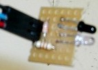
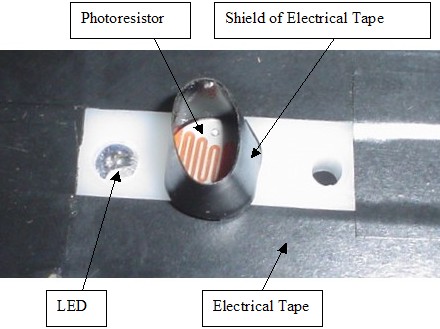
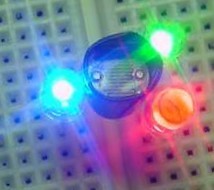
With a photoresistor, here is an example of where I used a green LED with a photoresistor shielded
with black electrical tape:
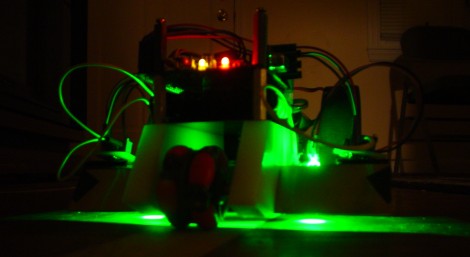
One advantage to having bright LEDs on your robot for color sensing is that your robot can look really
cool when the lights are off. This is what my undocumented secret 2006
MOBOT,
which used color sensing for line detection, looked like:
And of course if you wanted three different colors it would look something like this:
Programming your color sensor is very easy. You simply turn on a LED with a digital output pin,
wait about 50ms for the photoresistor to change (photoresistors are much much slower than
infrared sensors), take a reading with an analog pin,
then turn off the LED (if you have more than one LED).
For example, if your robot has three different color LEDs, this would be your pseudocode:
turn on green LED
wait 50ms
record sensor reading G
turn off green LED
turn on red LED
wait 50ms
record sensor reading R
turn off red LED
turn on blue LED
wait 50ms
record sensor reading B
turn off blue LED
Now using a similarity-matching algorithm, with precalibrated numbers, your robot can then identify
the target.
Range Detection with Shades
What is the difference between bright green and dark green? The only difference is that with
bright green there are more electromagnetic waves being detected and/or emitted. For example,
suppose you have a green apple and your robot takes a green color measurement. Then you move
the apple an inch back and take another measurement. What will happen? Simple, less green light
from the apple will reach your sensor. So how is this useful? Range detection!
Going back to the previous chart, can you see how you can calculate distance from an object?
 Unfortunately your color range sensor won't have a range of more than a few inches at most, depending on the brightness
of your LED. You could of course use a green laser pointer for maximum range, or apply a trick I am about to show you.
This following trick employs the same method TV remotes use to increase sensor range. Normally, if you apply
a large amount of power to an LED to increase brightness it will fry. But what if you put a huge amount of power
into it but over a very short period of time? Then you could make it say 5x brighter for ~5x increase in range!
Power (watts) is voltage x current. A typical LED can only work at a few 100 milliwatts before they fry (check your
datasheet) - this is why you should always put a resistor in series with an LED!
Now watts is a measurement of energy divided by time: energy/second. So what if we had the LED shine for only 50ms?
Well, that's 1 / .05 = 20, or 1/20th of a second. This means that if you shine your LED for only 50ms, then it can
take about 10 to 20 times more current, and therefore shine about 10 to 20 times brighter.
The exact numbers would depend on the thermal cooling rate of the LED - something that can only be determined by frying
a few LEDs with testing . . . Just so you know, its quite common to find half an amp going through a TV remote IR emitter!
Unfortunately your color range sensor won't have a range of more than a few inches at most, depending on the brightness
of your LED. You could of course use a green laser pointer for maximum range, or apply a trick I am about to show you.
This following trick employs the same method TV remotes use to increase sensor range. Normally, if you apply
a large amount of power to an LED to increase brightness it will fry. But what if you put a huge amount of power
into it but over a very short period of time? Then you could make it say 5x brighter for ~5x increase in range!
Power (watts) is voltage x current. A typical LED can only work at a few 100 milliwatts before they fry (check your
datasheet) - this is why you should always put a resistor in series with an LED!
Now watts is a measurement of energy divided by time: energy/second. So what if we had the LED shine for only 50ms?
Well, that's 1 / .05 = 20, or 1/20th of a second. This means that if you shine your LED for only 50ms, then it can
take about 10 to 20 times more current, and therefore shine about 10 to 20 times brighter.
The exact numbers would depend on the thermal cooling rate of the LED - something that can only be determined by frying
a few LEDs with testing . . . Just so you know, its quite common to find half an amp going through a TV remote IR emitter!
Modulation
There is yet another method to increasing detectable range of your sensor called modulation. It's somewhat complex
so Ill write about it in another tutorial, but it requires a very fast sensor. Basically you switch your
emitter on/off really fast so your sensor can therefore ignore background noise. As such you need a fast sensor.
Infrared sensors respond within
microseconds, but unfortunately photoresistors respond within milliseconds (bad!). If you were to do modulation,
it would be better to use IR, such as a Sharp IR Rangefinder. Unless . . .
Unless you use these neat color sensors that are made by
TAOS.

These sensors can be bought for many different specific wavelengths in the visible spectrum, yet
have the frequency response rate of IR sensors! They also require zero interface electronics - just plug
them in to power and analog I/O and wallah! I've done
some experimentation with them, but found
the ones I bought were over-sensitive. In a dimly lit room they already max out in voltage =(
So this concludes my color sensor tutorial, I hope you learned something!
High Altitude Balloon Tutorial
= Simulations, Modeling, Mapping =
 Intro to Simulations, Modeling, and Mapping for Balloons
Before we even begin, if you've never used software simulators before, I
strongly encourage you
to first read my
tutorial on finite element analysis. It will explain
to you all the caveats about using software simulators. Links to more software can be found on the
external links page.
Predicting the Weather
I can't emphasize how important launch planning is. The very first step is to have a look at the jet stream.
There are various websites out there, but the one I recommend the most is this animated version:
ANIMATION of Jet Stream Forecasts
(click
Build Animation to see it in motion)
They also have a
jet stream animation of the northern hemisphere
in case you live somewhere other than north America.
 image: example of jet stream mapping
The arrows represent wind speed and direction.
Ideally you'd want to launch when you expect the arrows to be really
small. If you choose the launch date poorly, you could end up with
150mph winds blowing your project 300 miles away (that means a 600 mile
drive there and back). Or worse, if you live on the east coast, your
project will
land in the Atlantic Ocean. The jet stream is seasonal and typically
calmer during the summer.
note: On the flip side, some people intentionally try to fly
their balloons across the Atlantic to Europe - so the jet stream isn't
always a bad thing!
Weather Soundings Data
Wind speeds and directions can vary greatly with altitude. Knowing your general launch region in mind,
you now need to get exact wind speed data from what's called 'sonar soundings'. Typically it's paid for with your tax
dollars and useful for various industries - yet free for you to do whatever with it.
One place to get sounding data is here:
http://weather.uwyo.edu/upperair/sounding.html
Click the location on the map, and it'll give you a chart of data which you can play around with.
If you google around you can find several sites offering sounding data in various formats.
The sonar soundings will consist of a chart listing things like
temperature, pressure, wind speed, and humidity at various altitudes.
This info can not only help you prepare for insulation and testing and
to verify post-flight data,
but also support running flight trajectory prediction simulations. I
encourage you to plot that data in Excel to better visualize the
atmosphere.
Predicting Rain
You can also plan for rain. Launching in the rain is bad for obvious reasons.
Launching with winds above 10mph is bad as the balloon is hard to control during inflation.
And 100% cloud cover makes pictures from your cameras rather boring.
Now, don't just go to some weather site and read the prediction for that day. It'll say something useless like
'Wednesday Rain 60% chance', and then there won't be a single cloud in the sky the whole day.
What you need to do is think like a weatherman and learn how to read satellite maps.
To plan for rainy weather, I use this
animated map from Wunderground.
You can zoom to individual locations, and track cloud movement over a
period of days.
Click the animation triangle button and watch how the clouds form, the
directions they move, and the distance it travels over a set
period of time. With a little practice, you can predict rain with fairly
high accuracy.
It also has a future weather prediction option on the map, but I haven't
verified if it's accurate or not.
The weather soundings data will help you guestimate the cloud direction and wind intensity for that day, too.
note: Our team typically sets a launch date weeks in advance, but doesn't 100% confirm the launch date until a day
or two before. If the weather is bad, we just shift it to our second 'rain date' (already decided in advance).
Simulations
Before I go any further, keep in mind that simulations ARE NOT an exact
science. They are fairly crude and can be inaccurate by large
percentages.
If you input bad data, it'll output incorrect results. Garbage in
garbage out.
To simulate, you need to input the weather of the launch date - but
how do you know the weather of the future? We typically run simulations 2
or 3 days before to determine a launch location and plan logistics.
We then run another the night before to confirm the launch location, and
yet again early morning before driving out to the planned launch site.
We have had times where we were forced to make last minute changes.
Each simulation uses the latest predictions of weather, with accuracy
increasing as the launch date becomes nearer. It's also fun to run a
simulation
after recovery using actual weather data to see how accurate the simulator really was.
Typically a simulation can determine where it'll land within a ~15 mile radius.
After looking up the jet stream and deciding which day is best to fly, choose a launch region
based on the wind direction and speed. This will help you with the next steps later in this tutorial. The best way to do this
would be to open up
google maps and look within a 50 mile radius of where you live/work.
We'll be coming back to this later to choose a more specific location.
 Simulating the Balloon and Parachute Vertical Speeds
The first part of your flight involves the balloon going up. But how
fast does it go up? If it's in the jet stream for a long time,
where winds are very fast, your balloon will travel very far (a bad
thing).
ascent
How high does the balloon go before it pops?
If you fill the balloon with too little helium, it'll go up too slow and
not very high. Worst case, it might even become
neutrally buoyant at too low of an altitude and simply not burst at all.
If you fill it too much it'll go up very fast,
but it'll also pop faster because of increased expansion of the helium.
So given your goals of altitude and such, you need to decide how much
air to use.
Use this Balloon Burst Calculator
or this CUSF Balloon Burst Calculator.
Measure exactly how much your balloon package
weighs. Even small errors can add up in a simulator! A general rule of
thumb is that you want about 4 to 5 pounds of positive lift (PPL).
note: here is another ascent rate calculator
Remember to rerun your calculation using the exact measured lift on launch day.
descent
After your balloon pops your package will start falling. It will fall
through the jet stream, and the slower it falls, the farther it'll blow
with the wind. The descent rate depends on the weight of your package
and the design/size/shape of your parachute. There are various
parachute descent calculators
out there. Choose the one that best fits your parachute design for
highest accuracy. Be aware that the material porosity (a property that
is
difficult to experimentally measure) and air pressure for that
particular day affects results.
If you want really high accuracy, copy the exact design of a parachute and package weight that has flown before,
and then look at the actual descent data of that parachute.
Simulations will help you design your chute to be sufficient, but actual
experimental tests are the only way to get an exact descent rate.
You can find a very tall building and throw your package off the roof.
Film it to measure descent rate. But keep in mind that descent rate
changes with
air pressure -
there is no air at high altitudes to fill your parachute! This below video was made when we questioned the logic of using
a dual parachute system - would two parachutes get tangled up or naturally separate?
The video shows that a dual parachute system works great. The weight
(schoolbag with stuff inside) was about 4 lbs. It was hand-thrown in
front of the parachute.
Unfortunately that was the tallest building I had roof access (without
risking arrest!).
At the end of the video it was more of a blooper reel. But it shows what
happens when the weight is launched upside down, i.e. it still works.
note: Another person on our HacDC team hand-made those two parachutes.
Balloon Trajectory Simulation
Now it's time to start simulating.
To help visualize how the simulator works, picture wind speed being zero
at all times.
Your balloon will go up and then fall back down - 100% vertically.
Given your previously calculated ascent and descent rates, your balloon
will spend different amounts of
time at different altitudes.
The wind conditions are different at each altitude, as listed by the
sounding data.
As such, your balloon will move horizontally at those speeds and
directions for that set period of time at that set altitude.
It's simple math, but involves a large number of repetitive
calculations.
A simulator does all that math and spits out a predicted trajectory.
Overlay that trajectory on a map and you have a predicted landing
location.
Remember: garbage in garbage out. Give it good data, and it'll give you an accurate trajectory.
Let's start with a simple simulator:
Balloon Trajectory Forecaster
Type in the balloon pop altitude and exactly where you plan to launch it (get GPS coordinates from Google maps).
This simulator does
not account for your specific ascent/descent rates, but it should give you a general idea of what to expect.
It will output the result as a GoogleEarth KML file. Just open that up in
Google Earth and play around with the trajectory
to get an intuitive feel for it.
For a more fancy (but also more complicated to use) simulator, there is
Balloon Track. If anyone knows of a better simulator,
or wants to link a tutorial on any other simulators,
contact me. But DO NOT
email me on how to use it. Ask all your questions in the
forum.
Choosing the Launch Location
Now that you have the predicted balloon trajectory, look at your Google
map and find an exact location to launch from.
Any place within a ~50 mile radius of your simulated launch location
will result in the same general trajectory.
A public field with no trees to snag your balloon is good. The
trajectory should follow major highways (not back roads)
so you can easily follow the balloon. The trajectory should not cross
over lakes, rivers, mountains, airports, restricted air spaces
(like the White House, or military bases), etc. And finally, the
expected landing region should be near a major road that goes straight
home.
It's not easy! Your team is likely to spend hours debating on the
'perfect' launch location. But I'd argue this is a good thing -
if a later simulation result forces a change in launch location,
everyone would already be aware of the issues making re-planning rather
quick and painless.
After you've decided on your launch location, run one more simulation using the new coordinates to verify the trajectory.
The below video shows a balloon trajectory recorded from one of our balloon flights.
Notice that the path the balloon takes to go up is nearly the mirror image of the path the balloon takes when coming back down.
The only difference is that the rate of falling was 2x that of rising. You can use this knowledge
to predict the final landing location during mid-flight.
note: large features such as mountains could distort the predicted landing location
Plotting the Final Trajectory
Just like when you plotted the simulated path, you can also plot the actual path from the logged GPS coordinates.
To convert your GPS data to a Google Earth compatible KML file, use the
GPS Visualizer.
Double click the KML file it gives you and Google Earth will do its magic (see above video for demonstration).
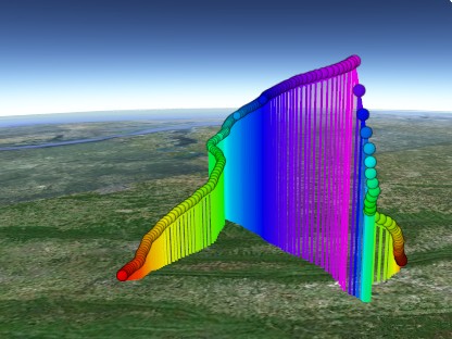
Below are the GPS coordinates plotted in 3D from our last flight, SB5.
Use your mouse to scroll around and inspect the trajectory. You need to have the latest version of
Google Earth
for it to work. If you don't, install it, then refresh this page.
|
|
BLUETOOTH WIRELESS
FOR ROBO |
|
What is Bluetooth?
Bluetooth is the USB of the wireless world. It is practically the standard now for personal
electronic wireless interfaces. You may already have heard of bluetooth being used in wireless
printers/scanners/mice/keyboards/headsets, digital cameras for image transfers to the PC,
some cordless phones, PDAs, and MP3 players.
Bluetooth makes the sharing and exchange of information between mobile and/or static devices as
simple as possible. Whether at home, on the move, or in the office it can be used for
networking, sharing files, synchronizing information, email, Internet access, printing, and more.
In industry it can be used to wirelessly control equipment and machinery - perfect for servicing
inaccessible devices.
And now it will be for a wireless link between a PC/laptop and your robot! Imagine reprogramming
your robot wirelessly (with bootloading software), or
data logging/collecting
sensor data, or sending commands without a long data cord to hassle with.
Way better than any
RC robot . . .
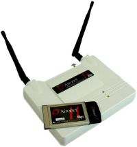
Here is a demonstration of setting up bluetooth on my
ERP
with an
Axon:
The Disadvantages of Wired Data Links
Let me say this bluntly - no cute girl would ever date you if you have a robot with a long
wire dragging behind it. Just that simple. And if that isnt enough, the wire will cause
locomotion resistance (imagine the wire pulling the robot back), will get tangled up in obstacles,
and has a limited length of only a few meters before signal degredation leads to signal failure.
Bluetooth Basics
Bluetooth is a license-free 2.4 GHz frequency band, usually with an integrated antenna,
having data-rates up to 3 Mbps (for Bluetooth v2.0), can pass through walls,
has easy setup, and optional data-encryption. Multiple links can be established concurrently
with different bluetooth devices because of automated frequency hopping (Frequency Hopping Spread Spectrum, or FHSS).
This is comparable to the creation of a virtual RS485-type bus allowing several devices to communicate at the same time.
What is FHSS? In this technique, a device will use 79 individual, randomly chosen frequencies within a designated range,
changing from one to another on a regular basis. In the case of Bluetooth, the transmitters change frequencies 1,600 times
every second, meaning that more devices can make full use of a limited slice of the radio spectrum. Since every Bluetooth
transmitter uses spread-spectrum transmitting automatically, it�s unlikely that two transmitters will be on the same
frequency at the same time. This same technique minimizes the risk that portable phones or baby monitors will disrupt
Bluetooth devices, since any interference on a particular frequency will last only a tiny fraction of a second.
 Classes of Bluetooth
Bluetooth comes in three classes.
Transmitting range cannot be explicitly stated for each device class; every environment is slightly
different, and affects the signal in different ways. The best way to compare a devices' operating range is by
comparing Output Power. A higher output power means a longer range.
Class 1 - Long Range
Maximum Output Power of 100mW (20dBm)
up to 100 meter range
Class 2 - Medium Range (the most common)
Maximum Output Power of 2.5mW (4dBm)
up to 10 meter range
Class 3 - Short Range (very rare)
Maximum Output Power of 1mW (0dBm)
up to ~1 meter range
Where Do I Connect Bluetooth On My Robot?
There are many different Bluetooth devices available on the market, but all are simple plug and play devices.
Just connect one directly to your
microcontroller
by either a
rs232 serial interface
or through the
UART tx/rx pins. I highly encourage you
to read my
microcontroller UART tutorial.
The easiest way to do this would buy a microcontroller that already has a built in serial interface, and then
connect it to a
rs232 bluetooth adaptor. I have found two by
brainboxes.com, and both are shown below.
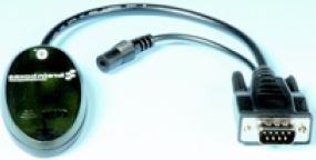
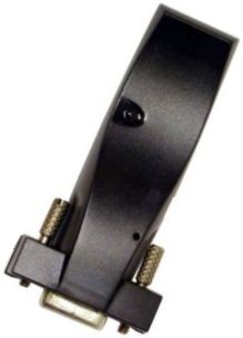
A Bluetooth rs232 Adaptor allows any device with an rs232 port to communicate with another Bluetooth
device without the need for additional software/drivers.
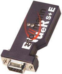
But as mentioned before, you could still get a
Bluetooth module and plug it directly into the micrcontrollers' UART pins.
Stollmann also offers many Bluetooth modules.
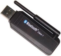
What About The Computer End?
The part that connects to your computer will be a
USB Bluetooth dongle. There are hundreds of
these on the market and are very easy/cheap to find and buy.

Notebooks can use Bluetooth via a PCMCIA card or a USB dongle.
There are Bluetooth adapters for PDAs and PDAs with integrated Bluetooth functionality.
There are also Bluetooth enabled phones (robot controlled by your mobile, anyone?).
Because the Bluetooth module basically acts like a wireless serial cable,
the software on the connected devices does not typically need to be modified.
 Extra Information - WiFi vs Bluetooth
What are the differences between WiFi and Bluetooth?
IEEE 802.11b offers faster speeds and greater range than Bluetooth.
While Bluetooth has a weaker radio signal, this provides for more
conservative use of battery power (designed for PDAs, wearable headsets,
cell phones).
Wifi's stronger signal provides more range, but uses 10 to 100 times
more power than Bluetooth
(designed for notebook computers, where the additional current drain is
negligible).
The two systems share space.
But WiFi uses te 2.4 GHz radio band/Direct Sequence Spread Spectrum (DSS), not frequency hopping (FHSS) such as with Bluetooth.
Bluetooth also doesn't typically have an access point. Devices on a Bluetooth PAN communicate directly with one another.
IEEE 802.11b allows mobility over a very large area. When out of range of one IEEE 802.11b access point, another takes over.
In the unlicensed 2.4 GHz radio spectrum, and it is possible for
Bluetooth and IEEE 802.11b systems to interfere with one another.
The 2.4 GHz Industrial, Scientific, and Medical (ISM) radio band is 83
MHz wide.
The ISM band is also used by the HomeRF wireless networking system,
cordless analog and digital phones, microwave ovens, and some medical
equipment.
As is the case with most unlicensed radio bands, no one "owns" any
particular frequency in the band, so users must share the radio
spectrum.
Generally keeping the devices far from each other distance wise will
dramatically reduce interference - but dont worry too much, the FCC
requires
all of these devices to 'play nice' and be resistant to interference.
Extra Information - Why is it Called 'Bluetooth'?
Apparently it was named after Harald Bluetooth, the King of Denmark in
the late 900's. He united Denmark and part of Norway into a single
kingdom,
so supposedly thats the link. But then he got owned by his son. Look him
up
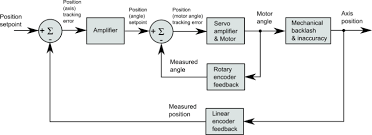
"This practical explanation helped me understand PID control better in two hours than a recent three-month theoretical course."
Has that PID controller that looks after your most important process always been a bit of a ‘black box?’
Have you Googled PID control and found that Wikipedia page with enough math to frighten Mr Spock?
My name is Finn Peacock, and I've been in the Control System
Engineering game for over 12 years. Over those 12 years I’ve repeatedly
been asked to explain how the PID controllers - on which million and
billion dollar enterprises depend - actually work.
After a lot of false starts I finally came up with not just an
analogy that explains PID control in plain English, but a series of
thought experiments. The great thing about thought experiments is that
they force you to VISUALIZE what’s going on.
And as almost every engineer I’ve ever met has a highly visual
mind - that means if you follow these thought experiments you should
never forget these fundamental PID Control concepts.
What Other Engineers Are Saying
“Easy to use and to follow. This is probably is
the best down-to-earth material for tuning PIDs that I have ever seen.
Really,..
it is Idiot Proof. It is like you just follow the lines painted on the floor and you will arrive safely at your destination.
Using your Blueprint,
my process was tuned with just PI. PID was not necessary after it was so well tuned. ”
"As I am rather new to this field of process control, I was very
pleased to have the PID Loop explained in a VERY understandable way (if
you know why, the how comes easy)
Now even I can explain it to others. Excellent Job!!!"
"I was impressed with how the your course explained all of the math
behind the proportional, integral and derivative terms in layman's
terms, so that operators, engineers, electricians, and mechanics cold
get a better understanding of PID control.
The Operators and Stationary Engineers in my plant were very
grateful that I allowed them to read the material, because now they
could understand the processes better.
I also liked the way that it built up each of the three
components, starting with proportional, then adding integral, then
finally adding derivative.
This practical explanation helped me understand PID
control better in two hours than I had learned in three-month
theoretical courses that I had taken in the past."
Thought I would edit this and put it back on the front page. There
seems to be quite a lot of PID talk at the moment, may be helpful to
someone.
I have built several robots which were capable of
avoiding obstacles and driving around without bumping into anything.
For a university project i wanted to make a robot that could build some
kind of map of it environment. During this project i found i needed
better control of my robot, to allow it to drive in a straight line and
follow walls. So i started experimenting with PID control. I thought i
would write a walkthrough to share what i have achieved.
Before
using PID control i was simply telling the robots wheels to drive at a
certain speed, set by a PWM output. I was then assuming that the robot
wheels would turn at the same speed and the robot would travel in a
straight line. This is known as open loop control. This means that you
send an output to the motors with no feedback and assume they travel at
the speed you set. It is very unlikely that two motors, even two
identical motors will turn at the same speed. So some sort of feedback
is required to control the speed. This is normally achieved using an
encoder. When the speed of the motor is controlled using feedback it is
known as closed loop control.
I have
implemented PID control to control both wheels of my robot, meaning the
wheels turn at the same speed and the robot can travel in a straight
line. I have also used it to allow my robot to follow walls. In this
case the feedback is not from the encoders on the motors but from a
sensor looking at the wall being followed. The idea behind PID control
is that you set a value that you want maintained, either a speed of a
motor of a reading from a sensor. You then take readings from the
encoder or the sensor and compare them to the setpoint. From this an
error value can be calculated, i.e,
(error = setpoint - actual reading).
This error value is then used to calculate how much to alter the motor
speed by to make the actual reading closer to the setpoint.
The
maths behind PID control can be pretty heavy. However, the process can
be simplified greatly if the frequency at which you sample the encoders
or the sensor is fixed. This is an important point and one that i wish
someone had told me when i started experimenting. I will now attempt to
explain how i implemented PID control, its quite a tricky thing to
explain so i will do my best and if anyone has any tips on how the
explanation can be improved, let me know and ill try again.
Ill
use an example of controlling one motor with encoder feedback to try
and explain how ive implemented PID control. I use an ATMEGA32 on my
robot, using 8bit PWM to drive a motor with an encoder that sends a
series of pulses as the motor turns. These pulses are counted by the
microcontroller. I use an internal interrupt that triggers when to
sample the encoder. I use a sampling time of around 1/10th of a second.
So i am taking a reading from the encoder 10 times a second, comparing
the reading to the setpoint to give me an error value, and using this
to calculate how much to alter the motor speed by.
So what do you
do with the error value to calculate how much to change the motor speed
by? i hear you ask. The simplest method is to simply add the error
value to the PWM output to change the motor speed. And this would work,
and is known as proportional control (the P in PID). It is often
necessary to scale the error value before adding it to the output by
using a gain contant. For example. Say the PWM output to the motor is
200, you have chosen a setpoint of 10. You are therefore expecting that
when you sample the encoder it should have sent 10 pulses to the
microcontroller since last time you sampled it. If the has only sent 6
pulses the motor is going to slow. The error (the difference between the
actual reading and the setpoint) is therefore 4. You could add this
value straight to the PWM output (200+4=204), which would speed up the
motor. It may take many samples before the motor speed matched the
setpoint, so it may be necessary to scale the error value, by
multiplying it by 2 for example. This would improve the response time.
As an equation this would look something like this:
c = E*Kp
where
c is the value to be added to the PWM output, E is the error value and
Kp is the gain constant. You only ever have to add c to the PWM output
as if the motor was going to fast, the error value would be negative,
and therefore c would also be negative.
AS
i mentioned this approach would work, but you may find that if you want
a quick response time, by using a large gain constant, or the error is
very large, the motor speed will go much higher than the setpoint, known
as overshoot. The motor speed may then go much lower than the
setpoint, then higher again and so on. When this approach is used on a
robot, the robot tends to oscillate in a jerky manner. This is when the
D bit of the PID comes into play. D stands for Derivative. It is used
to look at the rate of change of the error, i.e is the error changing
quickly of slowly. Another error value is calculate which i call Ed,
which is the difference between the previous error and the current error
(Ed = E - Eprev). This gives a value that is larger
if the error is changing quicky and a smaller value if the error is
changing slowly. If this is used as well as the proportial control it
is known as PD control, and an equation like this can be used:
c = (E*Kp)+(Ed*Kd)
where c, E and Kp are the same as before, Ed is calculated as shown above and Kd is the derivative gain constant.
The
I bit of PID refers to Integral control. I have found that generally
PD control is sufficient for controlling motor speeds and gives a good
performance. The integral control improves steady state perfomance,
that is when the motor speed has settled to a fairly consistant speed,
how far away from the setpoint is it running. By adding together all
prevoius errors it is possible to monitor if there are accumulating
errors. As if the motor is turning stightly too fast all the time, the
error will always be positive so the sum of the errors will get bigger,
the inverse is true if the motor is always going to slowly. An addition
error value, which i call Ei is simply the sum of all previous error.
This can be added into the equation, again with a gain contant to give
the full PID equation:
c = (E*Kp)+(Ed*Kd)+(Ei*Ki)
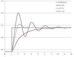
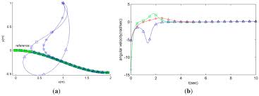
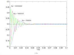
The
values of the K gain contants affect how much of each error are used to
alter the motor speed. Their values are usually found by trial and
error. To give an example the picture i have used for this walkthrough
is a graph of actual encoder values taken from my robot when it is
moving, with a setpoint of 10, You can see that the readings increase
above 10, oscillate around 10, before settling to around 10. This is a
common PID control loop response. I used settings of:
Kp = 1
Kd = 0.5
Ki = 0.3
I
hope this is helpful, as i said it is quite a tricky thing to explain
and im not sure i have done a very good job, please ask if there is
something i have not explained very well and i will try and improve it.
The
example i have given using a motor and an encoder is just one
application. If using a sensor to follow a wall the error value can be
calculated from the sensor reading compared to a setpoint. I have done
this using my two wheeled robot and just altered the speed of one wheel
while the other ran at a set speed. It worked very well using just PD
control. To make my two wheeled robot go in a straight line is had to
alter the speed of both wheels. To do this i sampled the left and right
encoders, and found an error value for each. I then put these values
into the PID equation and found a value to add to each motor.
Below
is the code i have used to control two motors on my robot. the doPID
loop is called everytime the encoders are sampled and the motor speeds
altered.
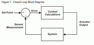
What is PID?
“PID”
is an acronym for Proportional Integral Derivative. As the name
suggests, these terms describe three basic mathematical functions
applied to the error (error = SetVal - SensorVal, where SetVal is the
target value and SensorVal is the present input value obtained from the
sensor ). Main task of the PID controller is to minimize the error of
whatever we are controlling. It takes in input, calculates the deviation
from the intended behaviour and accordingly adjusts the output so that
deviation from the intended behaviour is minimized and greater accuracy
obtained.
Why implement PID?
Line
following seems to be accurate when carried out at lower speeds. As we
start increasing the speed of the robot, it wobbles a lot and is often
found getting off track.
Hence some kind of control on the robot is
required that would enable us to make it follow the line efficiently at
higher speeds. This is where PID controller shines.
In order to implement line following one can basically start with just three sensors which are so spaced on the robot that-
- If the centre sensor detects the line the robot steers forward
- If the left sensor detects the line the robot steers right
- If the right sensor detects the line the robot steers left.
This
algorithm would make the robot follow the line, however, we would need
to compromise with its speed to follow the line efficiently.
We can increase the efficiency of line following by increasing the number of sensors, say 5.
Here the possible combinations represent exact position like-
| 00100 | On the centre of the line |
| 00001 | To the left of the line |
| 10000 | To the right of the line |
There
will be other possible combinations such as 00110 and 00011 that can
provide us data on how far to the right is the robot from the centre of
the line(same follows for left). Further to implement better line
following we need to keep track of how long is the robot not centered on
the line and how fast does it change its position from the centre.This
is exactly what we can achieve using “PID” control.The data obtained
from the array of sensors would then be put into utmost use and line
following process would be much more smoother, faster and efficient at
greater speeds.
PID is all about improving our control on the robot.
The
idea behind PID control is that we set a value that we want maintained,
either speed of a motor or reading from a sensor. We then take the
present readings as input and compare them to the setpoint. From this an
error value can be calculated, i.e, (error = setpoint - actual
reading). This error value is then used to calculate how much to alter
the output by to make the actual reading closer to the setpoint.
How to implement PID?
Terminology:
The basic terminology that one would require to understand PID are:
- Error
- The error is the amount at which a device isn’t doing something
right. For example, suppose the robot is located at x=5 but it should be
at x=7, then the error is 2.
- Proportional (P) - The proportional term is directly proportional to the error at present.
- Integral (I) - The integral term depends on the cumulative error made over a period of time (t).
- Derivative (D) - The derivative term depends rate of change of error.
- Constant
(factor)- Each term (P, I, D) will need to be tweaked in the code.
Hence,they are included in the code by multiplying with respective
constants.
- P-Factor (Kp) - A constant value used to increase or decrease the impact of Proportional
- I-Factor (Ki) - A constant value used to increase or decrease the impact of Integral
- D-Factor (Kd) - A constant value used to increase or decrease the impact of Derivative
Error measurement: In
order to measure the error from the set position, i.e. the centre we
can use the weighted values method. Suppose we are using a 5 sensor
array to take the position input of the robot. The input obtained can be
weighted depending on the possible combinations of input. The weight
values assigned would be such that the error in position is defined both
exactly and relatively.
The full range of weighted values is shown below. We assign a numerical value to each one.
| Binary Value | Weighted Value |
| 00001 | 4 |
| 00011 | 3 |
| 00010 | 2 |
| 00110 | 1 |
| 00100 | 0 |
| 01100 | -1 |
| 01000 | -2 |
| 11000 | -3 |
| 10000 | -4 |
| 00000 | -5 or 5 (depending on the previous value) |
The
range of possible values for the measured position is -5 to 5. We will
measure the position of the robot over the line several times a second
and use these value to determine Proportional, Integral and Derivative
values.
PID formula:
So what do we do
with the error value to calculate how much the output be altered by? We
would need to simply add the error value to the output to adjust the
robot’s motion. And this would work, and is known as proportional
control (the P in PID). It is often necessary to scale the error value
before adding it to the output by using the constant(Kp).
Proportional:
Difference = (Target Position) - (Measured Position)
Proportional = Kp*(Difference)
This
approach would work, but it is found that if we want a quick response
time, by using a large constant, or if the error is very large, the
output may overshoot from the set value. Hence the change in output may
turn out to be unpredictable and oscillating. In order to control this,
derivative expression comes to limelight.
Derivative:
Derivative
provides us the rate of change of error. This would help us know how
quickly does the error change from time to time and accordingly we can
set the output.
Rate of Change = ((Difference) – (Previous Difference))/time interval
Derivative= Kd *(Rate of Change)
The time interval can be obtained by using the timer of microcontroller.
The
integral improves steady state performance, i.e. when the output is
steady how far away is it from the setpoint. By adding together all
previous errors it is possible to monitor if there are accumulating
errors. For example- if the position is slightly to the right all the
time, the error will always be positive so the sum of the errors will
get bigger, the inverse is true if position is always to the left. This
can be monitored and used to further improve the accuracy of line
following.
Integral:
Integral = Integral + Difference
Integral = Ki*(Integral)
Summarizing “PID” control-
| Term | Expression | Effect |
| Proportional | Kp x error | It reduces a large part of the error based on present time error. |
| Integral | error dt | Reduces the final error in a system. Cumulative of a small error over time would help us further reduce the error. |
| Derivative | Kd x derror / dt | Counteracts the Kp and Ki terms when the output changes quickly. |
Therefore, Control value used to adjust the robot’s motion=
(Proportional) + (Integral) + (Derivative)
Tuning:
PID
implementation would prove to be useless rather more troublesome unless
the constant values are tuned depending on the platform the robot is
intended to run on. The physical environment in which the robot is being
operated vary significantly and cannot be modelled mathematically. It
includes ground friction, motor inductance, center of mass, etc. Hence,
the constants are just guessed numbers obtained by trial and error.
Their best fit value varies from robot to robot and also the
circumstance in which it is being run. The aim is to set the constants
such that the settling time is minimum and there is no overshoot.
There are some basic guidelines that will help reduce the tuning effort.
- Start
with Kp, Ki and Kd equalling 0 and work with Kp first. Try setting Kp
to a value of 1 and observe the robot. The goal is to get the robot to
follow the line even if it is very wobbly. If the robot overshoots and
loses the line, reduce the Kp value. If the robot cannot navigate a turn
or seems sluggish, increase the Kp value.
- Once the robot is
able to somewhat follow the line, assign a value of 1 to Kd (skip Ki for
the moment). Try increasing this value until you see lesser amount of
wobbling.
- Once the robot is fairly stable at following the
line, assign a value of 0.5 to 1.0 to Ki. If the Ki value is too high,
the robot will jerk left and right quickly. If it is too low, you won’t
see any perceivable difference. Since Integral is** cumulative, the Ki
value has **a significant impact. You may end up adjusting it by .01
increments.
- Once the robot is following the line with good
accuracy, you can increase the speed and see if it still is able to
follow the line. Speed affects the PID controller and will require
retuning as the speed changes.
Pseudo Code:Here is a simple loop that implements the PID control:
start:
error = (target_position) - (theoretical_position)
integral = integral + (error
dt)
derivative = ((error) - (previous_error))/dt
output = (Kperror) + (Ki
integral) + (Kdderivative)
previous_error = error
wait (dt)
goto start
Lastly,
PID doesn’t guarantee effective results just by simple implementation
of a code, it requires constant tweaking based on the circumstances,
once correctly tweaked it yields exceptional results. The PID
implementation also involves a settling time, hence effective results
can be seen only after a certain time from the start of the run of the
robot. Also to obtain a fairly accurate output it is not always
necessary to implement all the three expressions of PID. If implementing
just PI results yields a good result we can skip the derivative part.
What are Interrupts?
One of the most fundamental and useful principles of modern embedded processors are
interrupts.
An interrupt is a way for an external (or, sometimes, internal) event
to pause the current processor’s activity, so that it can complete a
brief task before resuming execution where it left off.
Example:
Let’s
say we are at home, writing an excellent tutorial on how a principle of
modern embedded processors works. We are very interested in this topic,
so we are devoting all our concentration to our keyboard. However, half
way though, the phone rings. Despite not being by the phone waiting for
a call, we are able to stop what we are doing, take the call, and go
back where we left off once we have hung up.
Consider
you’re at home watching an excellent movie(HD print). You are very much
interested in watching the end of the movie and suddenly the doorbell
rings. Now you have to pause your movie, get up from your chair, open
the door and then resume the movie form where you left it.
This
is how a microprocessor’s interrupt works. We can tell the processor to
look for some specific specific external event (like data reception
complete or pin changing its state like going from high to low) to
become true. While processor checks for these events we can parallely do
some other job. When these events occur, we stop the current task,
handle the interrupt, and resume back where we left off. This gives us a
great deal of flexibility. Rather that constantly checking the FLAG bit
via code we can trust interrupts to do the job of checking.
What we are doing is called
asynchronous
processing - that is, we are processing the interrupt events outside
the regular “execution thread” of the main program. The point to be
noted here is that we aren’t doing parallel programing (- running two or
more codes simultaneously) but we are just pausing the current program
and resuming to it after handing the interrupt.
We can link a specific interrupt source to a specific handler routine, called an
Interrupt Service Routine, or
ISR for short.
Interrupts available in AVR
There are two main sources of interrupts:
- Hardware
Interrupts : which occur in response to a changing external event such
as a pin going low, or a timer reaching a preset value
- Software Interrupts : which occur in response to a command issued in software
In
8-bit AVRs the software interrupts are not available, which are
basically used for generating user defined Exceptions and handling them
as and when they occur.
Each microcontroller has a set of interrupt sources available.
Some of the interrupts available in ATmega16 are as follows:
- External Interrupt
- Timer Interrupt
- USART Receive and Transmit Interrupt
- EEPROM Ready Interrupt
- ADC conversion complete
How do we handle Interrupts?
The method of handling interrupts differs in different languages.
For an Interrupt to fire ISR three things must be true
- The
AVR’s global Interrupts Enable bit must be set to one in the
microcontroller control register SREG. This allows the AVR’s core to
process interrupts via ISRs when set, and prevents them from running
when set to zero. It is like a global ON/OFF switch for the interrupts.
By default this bit is zero.
- The individual interrupt source’s
enable bit must be set. Each interrupt source has a separate interrupt
enable bit in the related peripherals control registers, which turns on
the ISR for that interrupt. This must also be set, so that when the
interrupt event occurs the processor runs the associated ISR.
- The
condition of the interrupt must be me - for example when the adc
conversion is complete then only it will fire ADC conversion interrupt.
When all three conditions are met, the AVR will fire our ISR each time the interrupt event occurs.
The C code for writing the ISR is as follows
pseudo C code:
#include <avr/interrupt.h>
ISR({Vector Source}_vect)
{
// ISR code to execute here
}
How do we enable an interrupt?
If
you simply add an ISR to your existing program, you will find that it
appears to do nothing when you try to fire it. This is because while we
have defined an ISR, we haven’t enabled the interrupt source.
Firstly,
we need to set the I bit in the SREG register. This is the Global
Interrupt Enable bit, without which the AVR will simply ignore any and
all interrupts.
In C, we can use predefined library functions. In
the case of AVR-GCC we just use the sei() and cli() macro equivalents
defined in <avr/interrupt.h>:
pseudo C code:
sei(); // Enable Global Interrupts
cli(); // Disable Global Interrupts
Now,
we need to enable a specific interrupt source, to satisfy the second
condition for firing an ISR. The way to do this varies greatly between
interrupt sources, but always involves setting a specific flag in one of
the peripheral registers. Let’s set an interrupt on the
USART Receive Complete (USART RX) interrupt. According to the datasheet, we want to set the RXCIE bit in the UCSRB register:
pseudo C code:
After sei(); and setting RXCIE the ISR will code will run when the data receive is complete.
Some Important Points
There are a few things to keep in mind when using interrupts in your program:
Now
we have learnt what are interrupts in general. In the next tutorial we
will see how to implement specific interrupts like ADC Conversion
Complete Interrupt, External Interrupts, Timer Interrupts etc.