electronics equipment engineered feelings for The Cyberlink Mind AMNIMARJESLOW GOVERNMENT 91220017 LOR EL CYBERLINK MIND UNTO FEELINGS 02096010014 ELECTRON LJBUSAF XAM $$$$$$$$$$
Electronic Stylus
ELECTRONIC FEELINGS EQUIPMENT IS THE KEY :
Antennas & Propagation
Online tutorials about antennas, transmission lines and propagation. Learn this aspect of electronics online because a good understanding of what happens after a signal leaves a transmitter and before it enters the recever itself is essential for anyone involved in radio or wireles technology.
One of the key areas of any radio system is that part where the signal is transfered from the transmitter to the receiver. This involves the use of antennas or aerials to radiate the signal as an electromagnetic wave, and then there is the way that the electromagntic wave travels or propagates between the transmitting antenna and the receiving one. Thus antennas and propagation are key areas for any radio system .
Meteor scatter or meteor burst communications
- a summary, overview or tutorial covering the basics of Meteor Scatter or Meteor Burst Communications, a form of radio signal propagation often used at VHF.
Meteor scatter or meteor burst communications use a form of radio communications system that is dependent on radio signals being scattered or reflected by meteor trails.
Meteor scatter communications is a specialized form of propagation that can be successfully used for radio communications over paths that extend up to 1500 or 2000 km.
Meteor scatter or meteor burst communication provides form of radio propagation that can be sued when no other form of radio propagation may be available. While data has to be transmitted in bursts and there may be delays, it provides a very useful form of non-real-time communications that can be used in many circumstances.
Meteor burst / communication basics
Meteor scatter or meteor burst radio communications relies on the fact that meteors continually enter the Earth's atmosphere. As they do so they burn up leaving a trail of ionisation behind them. These trails which typically occur at altitudes between about 85 and 120 km can be used to "reflect" radio signals. In view of the fact that the ionisation trails left by the meteors are small, only minute amounts of the signal are reflected and this means that high powers coupled with sensitive receivers are often necessary.
Meteor scatter propagation uses the fact that vast numbers of meteors enter the Earth's atmosphere. It is estimated that around 10^12 meteors enter the atmosphere each day and these have a total weight of around 10^6 grams.
Fortunately for everyone living below, the vast majority of these meteors are small, and are typically only the size of a grain of sand. It is found that the number of meteors entering the atmosphere is inversely proportional to their size. For a tenfold reduction in size, there is a tenfold increase in the number entering the atmosphere over a given period of time. From this it can be seen that very few large ones enter the atmosphere. Although most are burnt up in the upper atmosphere, there are a very few that are sufficiently large to survive entering the atmosphere and reach the earth.
Meteor burst communication applications
Meteor scatter or meteor burst communications are used for a number of applications on frequencies normally between about 40 and 150 MHz.
They are used professionally for a number of data transfer applications, particularly when transferring data from remote unmanned sites to a base using a radio communications link. Nowadays using computer controlled systems, this form of radio communications can offer an effective alternative to other means, and especially where satellites may need to be used because of the cost.
In other applications, radio hams use meteor scatter as a form of long distance VHF radio signal propagation.
Meteor burst communications system
The trails of ionisation left by meteors are short lived, and therefore the communications used needs to be able to be able to detect when a path exists and send high speed data while the radio path exists between the transmitter and the receiver.
A typical meteor scatter communications system, or meteor burst communications system will operate in a number of stages. A transmitter or master station will send out a probe signal. This is typically coded to ensure that communications are secure and not corrupted
1) Meteor scatter system sends out probe signal
A meteor trail will appear at some point that enables the transmitted probe signal to be reflected back so that it is received by the remote station. When this occurs the remote station will decode the signal and it will in turn transmit back a coded signal to the master. This signal is in turn checked by the master.
2) Receiver receives probe signal from transmitter
Once the link has been verified, data can be exchanged in either or both directions. Data is transmitted at high speed and also with constant error checks as the link will only be able to support communications for a few tenths of a second. After this point the diffusion of the meteor trail will reduce the ion density to a point where it will not reflect the signal back and the link will be lost.
3) Receiver receives probe signal from transmitter
When the link is lost, the master station starts to transmit its coded probe signal searching for the next meteor trail that will be able to support communications.
4) Meteor scatter system sends out probe signal
Although the normal maximum range is around 1500 km, for extended ranges a relay system can be implemented. Here a station approximately half way between the two end points can operate in a store and forward mode, storing the received data and forwarding it on as the trails become available. Time taken for data to be sent across the overall link will obviously increase, but for most systems that would consider meteor burst communications, this should not be a problem.
Radio hams & meteor scatter
Radio hams also make widespread use of meteor scatter as a mode of propagation. Often contacts will be pre-arranged at a specific time and frequency. Alternatively when meteor showers are predicted, special calling frequencies will be used. Normally high gain directive antenna are used to enable a sufficient signal to noise ratio.
Often high speed Morse code transmissions are used, or other data modes are now available.
The use of meteor scatter enables radio hams to make contacts on VHF bands when no other forms of communication / propagation may be available.
Meteors & Meteor Showers
A summary of the different types or classifications of meteors used for meteor burst or meteor scatter and the main meteor showers.
Although it may appear that meteors would all be the same as they all come from space, they can be categorised in different ways.
Although not always true, the types of meteor trail that the different types tend to make is different and this means that the radio propagation characteristics are different.
It is possible to split the meteors entering the atmosphere into two categories. One category is those that are associated with meteor showers at particular times of the year. The other is the meteors that enter the atmosphere all the time that are known as sporadic meteors.
Meteor showers: It found that at specific times during the year, the number of meteors entering the atmosphere rises significantly as a result of meteor showers. They occur as the Earth's path passes through debris in its orbit around the Sun. Often these have been traced back to the passage of a comet. For some of the larger showers, the number of visible trails rise significantly allowing the casual observer to see a worthwhile of trails in an evening. Of the meteor showers, the Perseids shower in August is probably the best, and the Quadrantids in January also produces a large number of trails.
Shower meteors are characterised by what is termed their radiant. This is the point in the sky from which they appear to originate. The radiant is usually identified by the name of the constellation or major star in the area of the sky from which they appear to come, and this name is usually given to the shower itself. Apart from the main showers, there are hundreds and possibly thousands of smaller showers that have been recorded, often by amateur observers.
Sporadic Meteors: The greatest number of meteors entering the atmosphere arises from sporadic meteors. These are the space debris that exists within the universe and in our solar system. The majority of this debris arises from the vast amounts of material that is thrown out by the Sun into the universe. Unlike the shower meteors they enter in all directions and they do not have a radiant.
What is Radio Propagation: RF propagation
An understanding of what radio propagation is can be an essential tool for anybody involved or interested in radio technology.
Radio signals can travel over vast distances. However radio signals are affected by the medium in which they travel and this can affect the radio propagation or RF propagation and the distances over which the signals can propagate. Some radio signals can travel or propagate around the globe, whereas other radio signals may only propagate over much shorter distances.
Radio propagation, or the way in which radio signals travel can be an interesting topic to study. RF propagation is a particularly important topic for any radio communications system. The radio propagation will depend on many factors, and the choice of the radio frequency will determine many aspects of radio propagation for the radio communications system.
Accordingly it is often necessary to have a good understanding of what is radio propagation, its principles, and the different forms to understand how a radio communications system will work, and to choose the best radio frequencies.
Radio propagation definition
Radio propagation is the way radio waves travel or propagate when they are transmitted from one point to another and affected by the medium in which they travel and in particular the way they propagate around the Earth in various parts of the atmosphere.
Factors affecting radio propagation
There are many factors that affect the way in which radio signals or radio waves propagate. These are determined by the medium through which the radio waves travel and the various objects that may appear in the path. The properties of the path by which the radio signals will propagate governs the level and quality of the received signal.
Reflection, refraction and diffraction may occur. The resultant radio signal may also be a combination of several signals that have travelled by different paths. These may add together or subtract from one another, and in addition to this the signals travelling via different paths may be delayed causing distorting of the resultant signal. It is therefore very important to know the likely radio propagation characteristics that are likely to prevail. Professional superheterodyne receiver Image courtesy Icom UK
The distances over which radio signals may propagate varies considerably. For some radio communications applications only a short range may be needed. For example a Wi-Fi link may only need to be established over a distance of a few metres. On the other hand a short wave broadcast station, or a satellite link would need the radio waves to travel over much greater distances. Even for these last two examples of the short wave broadcast station and the satellite link, the radio propagation characteristics would be completely different, the signals reaching their final destinations having been affected in very different ways by the media through which the signals have travelled.
Types of radio propagation
There are a number of categories into which different types of RF propagation can be placed. These relate to the effects of the media through which the signals propagate.
Free space propagation: Here the radio waves travel in free space, or away from other objects which influence the way in which they travel. It is only the distance from the source which affects the way in which the signal strength reduces. This type of radio propagation is encountered with radio communications systems including satellites where the signals travel up to the satellite from the ground and back down again. Typically there is little influence from elements such as the atmosphere, etc. . . . . Read more about free space propagation.
Ground wave propagation: When signals travel via the ground wave they are modified by the ground or terrain over which they travel. They also tend to follow the Earth's curvature. Signals heard on the medium wave band during the day use this form of RF propagation. Read more about ground wave propagation
Ionospheric propagation: Here the radio signals are modified and influenced by a region high in the earth's atmosphere known as the ionosphere. This form of radio propagation is used by radio communications systems that transmit on the HF or short wave bands. Using this form of propagation, stations may be heard from the other side of the globe dependent upon many factors including the radio frequencies used, the time of day, and a variety of other factors. . . . . Read more about ionospheric propagation.
Tropospheric propagation: Here the signals are influenced by the variations of refractive index in the troposphere just above the earth's surface. Tropospheric radio propagation is often the means by which signals at VHF and above are heard over extended distances. Read more about tropospheric propagation
In addition to these main categories, radio signals may also be affected in slightly different ways. Sometimes these may be considered as sub-categories, or they may be quite interesting on their own.
Some of these other types of niche forms of radio propagation include:
Sporadic E: This form of propagation is often heard on the VHF FM band, typically in summer and it can cause disruption to services as distant stations are heard. Read more about sporadic E propagation.
Meteor scatter communications: As the name indicates, this form of radio propagation uses the ionised trails left by meteors as they enter the earth’s atmosphere. When data is not required instantly, it is an ideal form of communications for distances around 1500km or so for commercial applications. Radio amateurs also use it, especially when meteor showers are present. Read more about meteor scatter communications.
Transequatorial propagation, TEP: Transequatorial propagation occurs under some distinct conditions and enables signals to propagate under circmstances when normal ionospheric propagation paths would not be anticipated.Read more about transequatorial propagation.
Near Vertical Incidence Skywave, NVIS: This form of propagation launches skywaves at a high angle and they are returned to Earth relatively close by. It provides local coverage in hilly terrain. Read more about NVIS propagation.
Auroral backscatter: The aurora borealis (Northern Lights) and Aurora Australis (Southern Lights) are indicators of solar activity which can disrupt normal ionospheric propagation. This type of propagation is rarely used for commercial communications as it is not predictable but radio amateurs often take advantage of it. Read more about auroral backscatter propagation.
Moonbounce EME: When high power transmissions are directed towards the moon, feint reflections can be heard if the antennas have sufficient gain. This form of propagation can enable radio amateurs to communicate globally at frequencies of 140 MHz and above, effectively using the Moon as a giant reflector satellite.
In addition to these categories, many short range wireless or radio communications systems have RF propagation scenarios that do not fit neatly into these categories. Wi-Fi systems, for example, may be considered to have a form of free space radio propagation, but there will be will be very heavily modified because of multiple reflections, refractions and diffractions. Despite these complications it is still possible to generate rough guidelines and models for these radio propagation scenarios.
RF propagation summary
There are many radio propagation scenarios in real life. Often signals may travel by several means, radio waves travelling using one type of radio propagation interacting with another. However to build up an understanding of how a radio signal reaches a receiver, it is necessary to have a good understanding of all the possible methods of radio propagation. By understanding these, the interactions can be better understood along with the performance of any radio communications systems that are used.
Radio Signal Path Loss
The intensity of radio waves and all electromagnetic waves diminishes with distance – there are many reasons for this which affect radio propagation.
Radio path loss is key factor in the design of any radio communications system or wireless system.
It is a fact that any radio signal will suffer attenuation when it travels from the transmitter to the receiver. A variety of different phenomena give rise to this radio path loss.
Understanding what causes radio path loss enables any system to be designed to perform to its best despite the various issues affecting it.
How does radio path loss affect systems
The radio signal path loss will determine many elements of the radio communications system in particular the transmitter power, and the antennas, especially their gain, height and general location. This is true for whatever frequency is used.
To be able to plan the system, it is necessary to understand the reasons for radio path loss, and to be able to determine the levels of the signal loss for a given radio path.
The radio path loss can often be determined mathematically and these calculations are often undertaken when preparing coverage or system design activities. These depend on a knowledge of the signal propagation properties.
Accordingly, radio path loss calculations are used in many radio and wireless survey tools for determining signal strength at various locations. These wireless survey tools are being increasingly used to help determine what radio signal strengths will be, before installing the equipment. For cellular operators radio coverage surveys are important because the investment in a macrocell base station is high. Also, wireless survey tools provide a very valuable service for applications such as installing wireless LAN systems in large offices and other centres because they enable problems to be solved before installation, enabling costs to be considerably reduced. Accordingly there is an increasing importance being placed onto wireless survey tools and software.
Radio path loss basics
The signal path loss is essentially the reduction in power density of an electromagnetic wave or signal as it propagates through the environment in which it is travelling.
There are many reasons for the radio path loss that may occur:
Free space loss: The free space loss occurs as the signal travels through space without any other effects attenuating the signal it will still diminish as it spreads out. This can be thought of as the radio communications signal spreading out as an ever increasing sphere. As the signal has to cover a wider area, conservation of energy tells us that the energy in any given area will reduce as the area covered becomes larger.
Diffraction: radio signal path loss due diffraction occurs when an object appears in the path. The signal can diffract around the object, but losses occur. The loss is higher the more rounded the object. Radio signals tend to diffract better around sharp edges, i.e. edges that are sharp with respect to the wavelength.
Multipath: In a real terrestrial environment, signals will be reflected and they will reach the receiver via a number of different paths. These signals may add or subtract from each other depending upon the relative phases of the signals. If the receiver is moved the scenario will change and the overall received signal will be found vary with position. Mobile receivers (e.g. cellular telecommunications phones) will be subject to this effect which is known as Rayleigh fading.
Absorption losses: Absorption losses occur if the radio signal passes into a medium which is not totally transparent to radio signals. There are many reasons for this which include:
Buildings, walls, etc: When radio signals pass through dense materials such was walls, buildings or even furniture within a building, they suffer attenuation. It is particularly applicable to cellular communications – in buildings, houses, etc signals are considerably reduced. The radio signal attenuation is more pronounced for the higher frequency mobile bands., e.g. 2.2 GHz as opposed to 800 / 900 MHz.
Atmospheric moisture: At high microwave frequencies radio path loss increases as a result of precipitation or even moisture in the air. The radio signal path loss may vary according to the weather conditions. However this typically only has a noticeable effect further into the microwave region.
Vegetation: In dense forest it is found that signals even at lower frequencies are considerably reduced. This illustrates that vegetation can introduce considerable levels of radio path loss. Trees and foliage can attenuate radio signals, particularly when wet.
Terrain: The terrain over which signals travel will have a significant effect on the signal. Obviously hills which obstruct the path will considerably attenuate the signal, often making reception impossible. Additionally at low frequencies the composition of the earth will have a marked effect. For example on the Long Wave band, it is found that signals travel best over more conductive terrain, e.g. sea paths or over areas that are marshy or damp. Dry sandy terrain gives higher levels of attenuation.
Atmosphere: The atmosphere can affect radio signal paths.
Ionosphere: At lower frequencies, especially below 30 - 50MHz, the ionosphere has a significant effect, reflecting (or more correctly refracting) them back to Earth. However when passing through some regions, especially the D region and to a lesser extent the E region, signals can suffer attenuation rather than reflection / refraction. This can introduce a significant radio path loss.
Troposphere: At frequencies above 50 MHz and more the troposphere has a major effect, refracting the signals back to earth as a result of changing refractive index. For UHF broadcast this can extend coverage to approximately a third beyond the horizon. The refraction can sometimes mean that signal that would normally reach a certain area may be refracted away from it.
These reasons represent some of the major elements causing signal path loss for any radio system.
Predicting radio path loss
One of the key reasons for understanding the various elements affecting radio signal path loss is to be able to predict the loss for a given path, or to predict the coverage that may be achieved for a particular base station, broadcast station, etc.
Although prediction or assessment can be fairly accurate for the free space scenarios, for real life terrestrial applications it is not easy as there are many factors to take into consideration, and it is not always possible to gain accurate assessments of the effects they will have.
Despite this there are wireless survey tools and radio coverage prediction software programmes that are available to predict radio path loss and estimate coverage. A variety of methods are used to undertake this.
Free space path loss varies in strength as an inverse square law, i.e. 1/(range)2, or 20 dB per decade increase in range. This calculation is very simple to implement, but real life terrestrial calculations of signal path loss are far more involved. To show how a real life situation can alter the calculations, often mobile phone operators may modify the inverse square law to 1/(range)n where n may vary between 3.5 to 5 as a result of the buildings and other obstructions between the mobile phone and the base station.
Most path loss predictions are made using techniques outlined below:
Statistical methods: Statistical methods of predicting signal path loss rely on measured and averaged losses for typical types of radio links. These figures are entered into the prediction model which is able to calculate the figures based around the data. A variety of models can be used dependent upon the application. This type of approach is normally used for planning cellular networks, estimating the coverage of PMR (Private Mobile Radio) links and for broadcast coverage planning.
Deterministic approach: This approach to radio signal path loss and coverage prediction utilises the basic physical laws as the basis for the calculations. These methods need to take into consideration all the elements within a given area and although they tend to give more accurate results, they require much additional data and computational power. In view of their complexity, they tend to be used for short range links where the amount of required data falls within acceptable limits.
These wireless survey tools and radio coverage software packages are growing in their capabilities. However it is still necessary to have a good understanding of radio propagation so that the correct figures can be entered and the results interpreted satisfactorily.
For any given radio transmission, the radio path loss is likely to be caused by a number of different factors. This often makes accurate radio path loss calculations difficult. However even if they are not as accurate as might be always liked, the radio path loss calculations enable equipment to be designed to meet the requirement
Free Space Path Loss: details & calculator
The simplest scenario for radio signal propagation is free space propagation model when a signal travels in free space.
The way the signal propagates and the path loss incurred provide a foundation for more complicated propagation models.
Although in most cases the free space propagation model details the way in which a radio signal travels in free space, when it is not under the influence of the many other external elements that affect propagation.
Free space propagation basics
The free space propagation model is the simplest scenario for the propagation of radio signals. Here they are considered to travel outwards from the point where they are radiated by the antenna.
The way in which they propagate can be likened to the ripples of waves on a pond that travel outwards from the point where a stone is dropped into a pond.
As the ripples move outwards their level reduces until they finally disappear to the eye.
In the case of radio signal propagation, the waves spread out in three dimensions rather than the two dimensions of the pond example.
Free space propagation signal level
It can be shown that the level of the signal falls as it moves away from the point where it has been radiated. Signals reduce in intensity as they travel from the transmitterThe rate at which it falls is proportional to the inverse of the square of the distance.
Signal level=kd2
Where: k = constant d = distance from the transmitter
As a simple example this means that the signal level of a transmission will be a quarter of the strength at 2 metres distance that it is at 1 metre distance.
Where a radio signal comes under the influence of other factors, the basic formula can be altered to take account of this.
The exponent is altered to represent more accurately the real life scenario. In environments like the internals of buildings such as buildings, stadiums and other indoor environments, the path loss exponent can reach values in the range of 4 to 6. Many mobile phone operators base their calculations on a terrestrial signal reduction around the inverse of the distance to the power 4. However tunnels can act as a form of waveguide and they can result in a path loss exponent values of less than 2.
Free space path loss calculation
It is possible to calculate the path loss between a transmitter and a receiver. The path loss proportional to the square of the distance between the transmitter and receiver as seen above and also to the square of the frequency in use.
The free space path loss can be expressed in terms of either the wavelength or the frequency. Both equations are given below:
In terms of wavelength
FSPL=(4πdλ)2
In terms of frequency
FSPL=(4πdfc)2
Where: FSPL = Free space path loss d = distance from the transmitter to the receiver (metres) λ = signal wavelength (metres) f = signal frequency (Hz) c = speed of light (metres per second)
Free space loss formula frequency dependency
The free space loss equations above seem to indicate that the loss is frequency or wavelength dependent. In reality the attenuation resulting from the distance travelled in space is not frequency or wavelength dependent and is constant.
Looking at the free space path loss equations it is possible to see that the result is dependent upon two effects:
The first results from the spreading out of the energy as the sphere over which the energy is spread increases in area. This is described by the inverse square law.
The second effect results from the antenna aperture change and this is dependent upon physical size and the wavelength being used. This affects the way in which any antenna can pick up signals and it results in this element being frequency dependent.
Even though one element of the equation for free space path loss is non-frequency dependent, the other is and this results in the overall equation having a wavelength or frequency dependence.
Free space path loss equation in deciBels
It is normally more convenient to be able to express the path loss in terms of a direct loss in decibels. In this way it is possible to calculate elements including the expected signal, etc.
The equation below shows the path loss for a free space propagation application. It can also be used when calculating or estimating other paths as well.
FSPL(dB)=20log(d)+20log(f)+32.44
Where: d = distance of the receiver from the transmitter (km) f = signal frequency (MHz) It is worth noting that the equation above does not include antenna gains and feeder losses. It is for two isotropic antennas, i.e. ones that radiate equally in all directions.
It is possible to add the antenna gains into the equation
F=20log(d)+20log(f)+32.44−Gtx−Grx
Where: Gtx = overall transmitter antenna gain including feeder losses Grx = overall receiver antenna gain including feeder losses
Free space path loss calculator
The simple free space path loss calculator is given below. To use the free space path loss calculator, enter the figures as required and press calculate to provide the answer.
As the IEEE "Standard Definitions of Terms for Antennas", IEEE 145-1983, states that a free space path loss is between two isotropic radiators. The calculator below is a path loss calculator because it includes the antenna gains. To make it a free space path loss calculator, antenna gains of 0 should be entered into both gain boxes.
Path Loss Calculator
Using the path loss calculator, it should be remembered that the calculations have been scaled to accept distances in terms of kilometres and frequencies in terms of MHz. All antenna gains are expressed in decibels relative to an isotropic radiator and not a dipole which has a gain of 2.1 dB over an isotropic source.
It should also be remembered that although the calculator is for path loss and is not strictly a free space path loss calculator, the calculation assumes there is free space between the two and no other effects affect the signal apart from the reduction due to signal distance and the antenna gains. A free space path loss calculation does not include the antenna gains and only looks at the path loss itself.
Radio Link Budget: details & formula
The radio link budget is a summary of transmitter power levels, system losses & gains.
When designing a complete, i.e. end to end radio communications system, it is necessary to calculate what is termed the radio link budget.
The link budget is a summary of the transmitted power long with all the gains and losses in the system and this enables the strength of the received signal to be calculated.
Using this knowledge it is possible to determine whether power and gain levels are sufficient, too high, or too low and then apply corrective action to ensure the system will operate satisfactorily.
This ensures that once the system is installed and is ready for operation, there will be sufficient signal for it to operate correctly, or whether the signal is too even high and action can be taken to save costs..
Larger than required antennas, high transmitter power levels and the like can add considerably to the cost, so it is necessary to balance these to minimise the cost of the system while still maintaining performance.
Link budgets are used in many applications from satellite links to mobile phone systems, HF radio links and many more.
Link budget style calculations are also used within wireless survey tools. These wireless survey tools will not only look at the way radio signals propagate, but also the power levels, antennas and receiver sensitivity levels required to provide the required link quality.
Radio link budget – the basics
As the name implies, a radio link budget is a summary of all the gains and losses in a transmission system. The radio link budget sums the transmitted power along with the gains and loses to determine the signal strength arriving at the receiver input. The link budget may include the following items:
Where the losses may vary with time, e.g. fading, and allowance must be made within the link budget for this - often the worst case may be taken, or alternatively an acceptance of periods of increased bit error rate (for digital signals) or degraded signal to noise ratio for analogue systems.
In essence the link budget will take the form of the equation below:
Received power (dBm)=Transmitted power (dBm)+Gains (dB)−Losses (dB)
The basic calculation to determine the link budget is quite straightforward. It is mainly a matter of accounting for all the different losses and gains between the transmitter and the receiver.
Once the link budget has been calculated, then it is possible to compare the calculated received level with the parameters for the receiver to discover whether it will be possible to meet the overall system performance requirements of signal to noise ratio, bit error rate, etc.
Radio link budget formula
In order to devise a radio link budget formula, it is necessary to investigate all the areas where gains and losses may occur between the transmitter and the receiver. Although guidelines and suggestions can be made regarding the possible areas for losses and gains, each link has to be analysed on its own merits.
A typical link budget equation for a radio communications system may look like the following:
PRX=PTX+GTX+GRX−LTX−LFS−LP−LRX
Where: PRX = received power (dBm) PTX = transmitter output power (dBm) GTX = transmitter antenna gain (dBi) GRX = receiver antenna gain (dBi) LTX = transmit feeder and associated losses (feeder, connectors, etc.) (dB) LFS = free space loss or path loss (dB) LP = miscellaneous signal propagation losses (these include fading margin, polarization mismatch, losses associated with medium through which signal is travelling, other losses...) (dB) LRX = receiver feeder and associated losses (feeder, connectors, etc.) (d)B
NB for the sake of visibility, the losses in the link budget equation is shown with a negative sign e.g. LTX or LFS, etc. When entering the figures into the radio link budget formula, the figure should be entered as the modulus of the loss. In this way they will be subtracted and not added to the figure.
Antenna gain & radio link budget
The basic link budget equation where no levels of antenna gain are included assumes that the power spreads out equally in all directions from the source, i.e. from an isotropic source, an antenna that radiates equally in all directions.
This assumption is good for many theoretical calculations, but in reality all antennas radiate more in some directions than others. In addition to this it is often necessary to use antennas with gain to enable interference from other directions to be reduced at the receiver, and at the transmitter to focus the available transmitter power in the required direction.
In view of this it is necessary to accommodate these gains into the link budget equation as they have been in the equation above because they will affect the signal levels - increasing them by levels of the antenna gain, assuming the gain is in the direction of the required link.When quoting gain levels for antennas it is necessary to ensure they are gains when compared to an isotropic source, i.e. the basic type of antenna assumed in the equation when no gain levels are incorporated. The gain figures relative to an isotropic source are quoted as dBi, i.e. dB relative to an isotropic source. Often gain levels given for an antenna may be the gain relative to a dipole where the figures may be quoted as dBd, i.e. dB relative to a dipole. However a dipole has gain relative to an isotropic source, so the dipole gain of 2.1 dBi needs to be accommodated if figures relative to a dipole are quoted for an antenna gain.
Link budget calculations are an essential step in the design of a radio communications system. The link budget calculation enables the losses and gains to be seen, and devising a link budget enables the apportionment of losses, gains and power levels to be made if changes need to be made to enable the radio communications system to meet its operational requirements. Only by performing a link budget analysis is this possible.
Radio Wave Reflection
Like other forms of electromagnetic wave, radio signals can be reflected by certain surfaces.
It is possible for radio waves to be reflected in the same way as light waves. As both light and radio waves are forms of electromagnetic waves, they are both subject to the same basic laws and principles.
Visual examples of light reflection are everywhere from specific mirrors to flat reflective surfaces like glass, polished metal and the like.
So too, radio waves can experience reflection.
Radio wave reflection
When a radio wave or in fact any electromagnetic wave encounters a change in medium, some or all of it may propagate into the new medium and the remainder is reflected. The part that enters the new medium is called the transmitted wave and the other the reflected wave.
The rules that govern the reflection of radio waves are simple and are the same as those that govern light waves. Propagation of reflected & refracted wavesWhen a reflection occurs it can be seen that the angle of incidence, θ1 is the same for the incident ray as for the reflected ray.
Additionally there is normally some loss, as a result of absorption, or signal passing into the medium.
Reflective medium
Conducting media provide the optimum surfaces for reflecting radio waves. Metal surfaces, and other conducting areas provide the best reflections. It is noticeable that for HF ionospheric propagation, when signals are returned to earth and are reflected back again by the Earth’s surface, areas of good conductivity provide the best reflections. Desert areas give poor reflected signals, but the sea is much better and the differences are very noticeable despite the variations in the ionosphere and overall propagation path.
Surface
Conductivity (Siemens)
Dry ground & desert
0.001
Average ground
0.005
Fresh water
0.01
Wet ground
0.02
Sea water
5
Multiple reflections
In real transmission paths, radio waves are often reflected by a variety of different surfaces. Although ionospheric reflections are actually caused by refraction, they can often be considered as reflections. Also for shorter range signals like mobile phone or other VHF / UHF communications the signals undergo many reflections.
These multiple reflections lead to the signal arriving at the receiver via several paths. Radio wave reflections normally give rise to multi-path effects.
The multiple reflections and multi-path effects give rise to distortion of the signal and fading.
When a signal arrives by two paths, one is longer than the other and will take longer to arrive than the other. This can mean that the signals either add together if they are in phase, or they can tend to cancel each other out. This results in fading of anything moves of changes, or dead spots in certain areas if the reflective surfaces are fixed.
Additionally the delays in some signal paths can give rise to distortion of the modulation. For audio the signal can literally sound distorted dependent upon the type of modulation used – frequency modulation the audio can become very broken when multiple signals are received. For digital signals, it can result in data becoming corrupt as the data from one path may be delayed compared to the other and the receiver not being able to distinguish where data bits start and stop.
Radio Wave Refraction
Like other forms of electromagnetic wave, radio signals can be refracted when the refractive index of the medium through which they are passing changes.
It is possible for radio waves to be refracted in the same way as light waves. As both light and radio waves are forms of electromagnetic waves, they are both subject to the same basic laws and principles.
The concept of refraction is generally illustrated in terms of light. On a hot day the surface of the ground can be heated and this causes air to rise. Hot air and the colder air have slightly different values of refractive index and this causes the light to bend. With the movement of the rising air the surface of the ground appears to shimmer.
Refraction of radio waves
In just the same way that light waves are refracted, so too radio waves can undergo refraction.
The classic case for refraction occurs at the boundary of two media. At the boundary, some of the electromagnetic waves will be reflected, and some will enter the new medium and be refracted. Propagation of reflected & refracted wavesThis is best illustrated by placing a straight stick through the surface of a still pond where both the reflection and the refracted waves can be seen.
Radio wave refraction follows exactly the same effects as it does for light.
The basic law for radio wave refraction and light wave refraction is known as Snells Law which states:
η1sin(θ1)=η2sin(θ2)
Gradual changes in refractive index
Rather than a sudden boundary to two different media, radio waves will often be refracted by areas where the refractive index gradually changes.
This may happen as the radio waves propagate through the atmosphere where small changes in refractive index occur.
Typically it is found that the refractive index of the air is higher close to the earth’s surface, falling slightly with height.
In this case the radio waves are refracted towards the area of higher refractive index. This extends the range over which they can travel.
Refraction of radio waves in ionised regions
Radio waves are also refracted in regions of ionisation such as the ionosphere.
The ionosphere is a region in the upper atmosphere where there is a large concentration of ions and free electrons, primarily as a result of the effect of the Sun’s radiation on the upper reaches of the atmosphere.
The electrons in the ionosphere are excited by the radio waves and are set in motion by them as a result they tend to re-radiate the signal. As the signal is travelling in an area where the density of electrons is increasing, the further it progresses into the region, the signal is refracted away from the area of higher electron density. In the case of signals below about 30 MHz, this refraction is often sufficient to bend them back to earth. In effect it appears that the region has "reflected" the signal.
The tendency for this "reflection" is dependent upon the frequency and the angle of incidence. As the frequency increases, it is found that the amount of refraction decreases until a frequency is reached where the signals pass through the region and on to the next. Eventually a point is reached where the signal passes through the E layer on to the next layer above it.
The state of the ionosphere is constantly changing, so the degrees of refraction that are encountered will vary continually.
Radio Wave Diffraction
Like other forms of electromagnetic wave, radio signals can be diffracted when they travel past sharp corners
Electromagnetic waves can be diffracted when they meet a sharp obstacle.
As radio waves are a form of electromagnetic wave, it means that they can also be diffracted.
Radio wave diffraction
As radio waves undergo diffraction it means that a signal from a transmitter may be received from a transmitter even though it may be "shaded" by a large object between them.
To understand how this happens it is necessary to look at Huygen's Principle. This states that each point on a spherical wave front can be considered as a source of a secondary wave front.
Even though there will be a shadow zone immediately behind the obstacle, the signal will diffract around the obstacle and start to fill the void. It is found that diffraction is more pronounced when the obstacle becomes sharper and more like a "knife edge".
For a radio signal the definition of a knife edge depends upon the frequency, and hence the wavelength of the signal.
For low frequency signals a mountain ridge may provide a sufficiently sharp edge. A more rounded hill will not produce such a marked effect. It is also found that low frequency signals diffract more markedly than higher frequency ones. It is for this reason that signals on the long wave band are able to provide coverage even in hilly or mountainous terrain where signals at VHF and higher would not. Radio wave diffraction The effect may also be important for very high frequency signals where items of furniture in the home may have a sufficiently sharp edge to enable diffraction to be seen. This may give slightly better coverage to items like mobile phones or for Wi-Fi systems.
Multipath Propagation
Multipath radio propagation affects virtually all wireless signals: it can give rise to interference or it can be used to increase improve performance with techniques like MIMO.
Multipath propagation is a fact of life in any terrestrial radio scenario. While the direct or line of sight path is often the main wanted signal, a radio receiver will receive different versions of the same signal that have travelled from the transmitter via many different paths.
Multipath propagation basics
The vast number of different signal paths arise from the fact that signals are reflections from buildings, mountains or other reflective surfaces including water, etc. that may be adjacent to the main path. Additionally other effects such as ionospheric reflections give rise to multipath propagation as does tropospheric ducting.
The antennas used for transmission and reception have an effect on the number of paths that the signal can take. Non-directive antennas will radiate the signal in all directions, whereas directive ones will focus the power in one direction reducing the strength of reflected signals away from the main beam.
The multipath propagation resulting from the variety of signal paths that may exist between the transmitter and receiver can give rise to interference in a variety of ways including distortion of the signal, loss of data and multipath fading.
At other times, the variety of signal paths arising from the multipath propagation can be used to advantage. Schemes such as MIMO use multipath propagation to increase the capacity of the channels they use or seek to improve the signal to noise ratio.
Multipath fading
Signals are received in a terrestrial environment, i.e. where reflections are present and signals arrive at the receiver from the transmitter via a variety of paths. The overall signal received is the sum of all the signals appearing at the antenna. Sometimes these will be in phase with the main signal and will add to it, increasing its strength. At other times they will interfere with each other. This will result in the overall signal strength being reduced.
Multipath fading: Multipath fading can be detected on many signals across the frequency spectrum from the HF bands right up to microwaves and beyond. It can cause signals to rise and fall in strength. . . . . . . Read more about multipath fading.
Rayleigh fading: Rayleigh fading is the name given to the form of fading that is often experienced in an environment where there is a large number of reflections present. . . . . . . Read more about Rayleigh fading.
Interference caused by multipath propagation
Multipath propagation can give rise to interference that can reduce the signal to noise ratio and reduce bit error rates for digital signals. One cause of a degradation of the signal quality is the multipath fading already described. However there are other ways in which multipath propagation can degrade the signal and affect its integrity.
One of the ways which is particularly obvious when driving in a car and listening to an FM radio. At certain points the signal will become distorted and appear to break up. This arises from the fact that the signal is frequency modulated and at any given time, the frequency of the received signal provides the instantaneous voltage for the audio output. If multipath propagation occurs, then two or more signals will appear at the receiver. One is the direct or line of sight signal, and another is a reflected signal. As these will arrive at different times because of the different path lengths, they will have different frequencies, caused by the fact that the two signals have been transmitted by the transmitter at slightly different times. Accordingly when the two signals are received together, distortion can arise if they have similar signal strength levels.
Another form of multipath propagation interference that arises when digital transmissions are used is known as Inter Symbol Interference, ISI. This arises when the delay caused by the extended path length of the reflected signal. If the delay is significant proportion of a symbol, then the receiver may receive the direct signal which indicates one part of the symbol or one state, and another signal which is indicating another logical state. If this occurs, then the data can be corrupted.
One way of overcoming this is to transmit the data at a rate the signal is sampled, only when all the reflections have arrived and the data is stable. This naturally limits the rate at which data can be transmitted, but ensures that data is not corrupted and the bit error rate is minimised. To calculate this the delay time needs to be calculated using estimates of the maximum delays that are likely to be encountered from reflections .
Multipath Fading
Multipath fading occurs when signals reach a receiver via many paths & their relative strengths & phases change.
Multipath fading affects most forms of radio communications links in one form or another.
Multipath fading can affect signals on frequencies from the LF portion of the spectrum and below right up into the microwave portion of the spectrum.
Multipath fading occurs in any environment where there is multipath propagation and the paths change for some reason. This will change not only their relative strengths but also their phases, as the path lengths will change.
Multipath fading may also cause distortion to the radio signal. As the various paths that can be taken by the signals vary in length, the signal transmitted at a particular instance will arrive at the receiver over a spread of times. This can cause problems with phase distortion and inter-symbol interference when data transmissions are made. As a result, it may be necessary to incorporate features within the radio communications system that enables the effects of these problems to be minimised.
Multipath fading basics
Multipath fading is a feature that needs to be taken into account when designing or developing a radio communications system. In any terrestrial radio communications system, the signal will reach the receiver not only via the direct path, but also as a result of reflections from objects such as buildings, hills, ground, water, etc that are adjacent to the main path.
The overall signal at the radio receiver is a summation of the variety of signals being received. As they all have different path lengths, the signals will add and subtract from the total dependent upon their relative phases.
At times there will be changes in the relative path lengths. This could result from either the radio transmitter or receiver moving, or any of the objects that provides a reflective surface moving. This will result in the phases of the signals arriving at the receiver changing, and in turn this will result in the signal strength varying as a result of the different way in which the signals will sum together. It is this that causes the fading that is present on many signals.
Selective and flat fading
Multipath fading can affect radio communications channels in two main ways. This can given the way in which the effects of the multipath fading are mitigated.
Flat fading: This form of multipath fading affects all the frequencies across a given channel either equally or almost equally. When flat multipath fading is experienced, the signal will just change in amplitude, rising and falling over a period of time, or with movement from one position to another.
Selective fading: Selective fading occurs when the multipath fading affects different frequencies across the channel to different degrees. It will mean that the phases and amplitudes of the signal will vary across the channel. Sometimes relatively deep nulls may be experienced, and this can give rise to some reception problems. Simply maintaining the overall amplitude of the received signal will not overcome the effects of selective fading, and some form of equalization may be needed. Some digital signal formats, e.g. OFDM are able to spread the data over a wide channel so that only a portion of the data is lost by any nulls. This can be reconstituted using forward error correction techniques and in this way it can mitigate the effects of selective multipath fading.
Selective multipath fading occurs because even though the path length will be change by the same physical length (e.g. the same number of metres, yards, miles, etc) this represents a different proportion of a wavelength. Accordingly the phase will change across the bandwidth used.
Selective fading can occur over many frequencies. It can often be noticed when medium wave broadcast stations are received in the evening via ground wave and skywave. The phases of the signals received via the two means of propagation change with time and this causes the overall received signal to change. As the multipath fading is very dependent on path length, it is found that it affects the frequencies over even the bandwidth of an AM broadcast signal to be affected differently and distortion results.
Selective multipath fading is also experienced at higher frequencies, and with high data rate signals becoming commonplace wider bandwidths are needed. As a result nulls and peaks may occur across the bandwidth of a single signal.
Cell phone signal fading
Mobile phone communications are subject to multipath fading. There are a variety of reasons for this.
Mobile user is moving:, The first is that the mobile station or user is likely to be moving, and as a result the path lengths of all the signals being received are changing. The second is that many objects around may also be moving. Automobiles and even people will cause reflections that will have a significant effect on the received signal. Accordingly multipath fading has a major bearing on cellular telecommunications.
Other objects moving: Often the multipath fading that affects cellular phones is known as fast fading because it occurs over a relatively short distance. Slow fading occurs as a cell phone moves behind an obstruction and the signal slowly fades out.
>The fast signal variations caused by multipath fading can be detected even over a short distance. Assume a frequency of 2 GHz (e.g. a typical approximate frequency value for many phones). The wavelength can be calculated as:
λ=cf
λ=3⋅1082⋅109
λ=0.15metres
Where: c = speed of light in metres per second f = frequency in Hertz
To move from a signal being in phase to a signal being out of phase is equivalent to increasing the path length by half a wavelength or 0.075m, or 7.5 cms. This example looks at a very simplified example. In reality the situation is far more complicated with signals being received via many paths. However it does give an indication of the distances involved to change from an in-phase to an out of phase situation.
Ionospheric fading
Short wave radio communications is renowned for its fading. Signals that are reflected via the ionosphere, vary considerably in signal strength. These variations in strength are primarily caused by multipath fading.
When signals are propagated via the ionosphere it is possible for the energy to be propagated from the transmitter to the receiver via very many different paths. Simple diagrams show a single ray or path that the signal takes. In reality the profile of the electron density of the ionosphere (it is the electron density profile that causes the signals to be refracted) is not smooth and as a result any signals entering the ionosphere will be scattered and will take multiple paths to reach a particular receiver. With changes in the ionosphere causing the path lengths to change, this will result in the phases changing and the overall summation at the receiver changing.
The changes in the ionosphere arise from a number of factors. One is that the levels of ionisation vary, although these changes normally occur relatively slowly, but nevertheless have an effect. In addition to this there are winds or air movements in the ionosphere. As the levels of ionisation are not constant, any air movement will cause changes in the profile of the electron density in the ionosphere. In turn this will affect the path lengths.
It is for this reason that signals on the short wave bands are constantly changing in strength.
Tropospheric fading
Many signals using frequencies at VHF and above are affected by the troposphere. The signal is refracted as a result of the changes in refractive index occurring, especially within the first kilometres above the ground. This can cause signals to travel beyond the line of sight. In fact for broadcast applications a figure of 4/3 of the visual line of sight is used for the radio horizon. However under some circumstances relatively abrupt changes in refractive index occurring as a result of weather conditions can cause the distances over which signals travel to be increased. Signals may then be "ducted" by the ionosphere over distances up to a few hundred kilometres.
When signals are ducted in this way, they will be subject to multipath fading. Here, heat rising from the Earth's surface will ensure that the path is always changing and signals will vary in strength. Typically these changes may be relatively slow with signals falling and rising in strength over a period of a number of minutes.
Multipath radio fading is factor that appears on most signals to a greater or lesser degree. As radio signals tend to reach a receiver via multiple paths regardless of how good the path appears to be there are always likely to be reflections from other objects. The only exception is in outer space where there are very few significant objects that are likely to cause major issues.
Rayleigh Fading
Rayleigh fading is the name given to the form of fading that is often experienced in an environment where there is a large number of reflections present.
The Rayleigh fading model uses a statistical approach to analyse the propagation, and can be used in a number of environments.
The Rayleigh fading model is ideally suited to situations where there are large numbers of signal paths and reflections. Typical scenarios include cellular telecommunications where there are large number of reflections from buildings and the like and also HF ionospheric communications where the uneven nature of the ionosphere means that the overall signal can arrive having taken many different paths.
The Rayleigh fading model is also appropriate for for tropospheric radio propagation because, again there are many reflection points and the signal may follow a variety of different paths.
Rayleigh fading definition
The Rayleigh fading model may be defined as follow:
Rayleigh fading model: Rayleigh fading models assume that the magnitude of a signal that has passed through such a transmission medium (also called a communications channel) will vary randomly, or fade, according to a Rayleigh distribution — the radial component of the sum of two uncorrelated Gaussian random variables.
Rayleigh radio signal fading basics
The Rayleigh fading model is particularly useful in scenarios where the signal may be considered to be scattered between the transmitter and receiver. In this form of scenario there is no single signal path that dominates and a statistical approach is required to the analysis of the overall nature of the radio communications channel.
Rayleigh fading is a model that can be used to describe the form of fading that occurs when multipath propagation exists. In any terrestrial environment a radio signal will travel via a number of different paths from the transmitter to the receiver. The most obvious path is the direct, or line of sight path.
However there will be very many objects around the direct path. These objects may serve to reflect, refract, etc the signal. As a result of this, there are many other paths by which the signal may reach the receiver.
When the signals reach the receiver, the overall signal is a combination of all the signals that have reached the receiver via the multitude of different paths that are available. These signals will all sum together, the phase of the signal being important. Dependent upon the way in which these signals sum together, the signal will vary in strength. If they were all in phase with each other they would all add together. However this is not normally the case, as some will be in phase and others out of phase, depending upon the various path lengths, and therefore some will tend to add to the overall signal, whereas others will subtract.
As there is often movement of the transmitter or the receiver this can cause the path lengths to change and accordingly the signal level will vary. Additionally if any of the objects being used for reflection or refraction of any part of the signal moves, then this too will cause variation. This occurs because some of the path lengths will change and in turn this will mean their relative phases will change, giving rise to a change in the summation of all the received signals.
The Rayleigh fading model can be used to analyse radio signal propagation on a statistical basis. It operates best under conditions when there is no dominant signal (e.g. direct line of sight signal), and in many instances cellular telephones being used in a dense urban environment fall into this category. Other examples where no dominant path generally exists are for ionospheric propagation where the signal reaches the receiver via a huge number of individual paths. Propagation using tropospheric ducting also exhibits the same patterns. Accordingly all these examples are ideal for the use of the Rayleigh fading or propagation model.
X . I Waveguide Microwave Feeder
Waveguides are RF feeders used at microwave frequencies where they are able to provide very low levels of loss.
Waveguides are a form of RF feeder or transmission line used at microwave frequencies.
A waveguide generally consists of a form of circular or rectangular conducting pie. As the name waveguide suggests, it confines and guides the electromagnetic wave within the walls of the feeder.
As the walls are made of a conductor such as brass, and they may even be silver plated, conduction losses are low, and the electromagnetic wave cannot escape the confines of the waveguide feeder. As a result the losses of waveguide feeders are very low when compared to other forms of feeder.
Waveguide feeder basics
Waveguides are used in a variety of applications to carry radio frequency energy from one point to another. In their broadest terms they can be described as a system of material that is designed to confine electromagnetic waves in a direction defined by its physical boundaries. This definition gives a very broad view of their properties, but it indicates that waveguide theory can be applied in a number of areas and in a variety of different ways.
Electromagnetic waves propagating in open space travel out in all directions and can be thought of as spherical waves travelling out from a central source. As a result the power intensity decreases as the distance increases - it is proportional to the power of the source divided by the square of the distance. The waveguide operates by confining the electromagnetic wave so that it does not spread out and losses resulting from this effect are eliminated.
Typically a waveguide is thought if as a transmission line comprising a hollow conducting tube, which may be rectangular or circular within which electromagnetic waves are propagated.
Unlike coaxial cable which is also a transmission line, there is no centre conductor within the waveguide. Signals propagate within the confines of the metallic walls that act as boundaries. The signal propagation is confined by total internal reflection from the walls of the waveguide. Rectangular waveguide
Circular waveguideWaveguides will only carry or propagate signals above a certain frequency, known as the cut-off frequency. Below this the waveguide is not able to carry the signals. This is obviously an important parameter, and one of the most basic specifications for its operation. It is for this reason that waveguides are typically only used at microwave frequencies.
Types of waveguide feeder
There is a number of different types of microwave waveguide that can be used, bought and designed.
Most waeguides are rectangular in cross section as this is the most common form of waveguide, but other types are available.
Rectangular waveguide: This is the most commonly used form of waveguide and has a rectangular cross section. The dimesions of the cross section sides determine the preperties including the cut-off frequency
Circular waveguide: This is less common than rectangular waveguide. They have many similarities in their basic approach, although signals often use a different mode of propagation. The diameter is important as this determines the operating range.
Circuit board stripline: This form of waveguide is used on printed circuit boards as a transmission line for microwave signals. It typically consists of a line of a given thickness above an earth plane. Its thickness defines the impedance.
In addition to these basic forms, there are also flexible waveguides. These are most widely seen in the rectangular format. Flexible waveguide is often used to connect to antennas, etc that may not be fixed or may be moveable.
Waveguide feeder advantages & disadvantages
Waveguide microwave feeder has a number of significant advantages, but it also has a number of disadvantages.
Waveguide feeder advantages:
Very low loss
Can operate at very high frequencies (microwaves)
Waveguide feeder disadvantages:
Expensive
Not flexible (there are some flexible types but these are particularly expensive
Requires special flanges and adaptors to join sections together.
Waveguide feeder is not as widely used as other forms of RF feeder like coax.
Waveguide Modes: TE, TM, TEM . .
Signals propagate within waveguides in a number of different ways or modes: TE, TM, TEM and they have different orders of each mode . . ..
Electromagnetic waves can travel along waveguides using a number of different modes.
The different waveguide modes have different properties and therefore it is necessary to ensure that the correct mode for any waveguide is excited and others are suppressed as far as possible, if they are even able to be supported.
Waveguide modes
Looking at waveguide theory it is possible it calculate there are a number of formats in which an electromagnetic wave can propagate within the waveguide. These different types of waves correspond to the different elements within an electromagnetic wave.
TE mode: This waveguide mode is dependent upon the transverse electric waves, also sometimes called H waves, characterised by the fact that the electric vector (E) being always perpendicular to the direction of propagation.
TM mode: Transverse magnetic waves, also called E waves are characterised by the fact that the magnetic vector (H vector) is always perpendicular to the direction of propagation.
TEM mode: The Transverse electromagnetic wave cannot be propagated within a waveguide, but is included for completeness. It is the mode that is commonly used within coaxial and open wire feeders. The TEM wave is characterised by the fact that both the electric vector (E vector) and the magnetic vector (H vector) are perpendicular to the direction of propagation.
Text about the different types of waveguide modes often indicates the TE and TM modes with integers after them: TEm,n. The numerals M and N are always integers that can take on separate values from 0 or 1 to infinity. These indicate the wave modes within the waveguide.
Only a limited number of different m, n modes can be propagated along a waveguide dependent upon the waveguide dimensions and format. Rectangular waveguide TE modesFor each waveguide mode there is a definite lower frequency limit. This is known as the cut-off frequency. Below this frequency no signals can propagate along the waveguide. As a result the waveguide can be seen as a high pass filter.
It is possible for many waveguide modes to propagate along a waveguide. The number of possible modes for a given size of waveguide increases with the frequency. It is also worth noting that there is only one possible mode, called the dominant mode for the lowest frequency that can be transmitted. It is the dominant mode in the waveguide that is normally used.
It should be remembered, that even though waveguide theory is expressed in terms of fields and waves, the wall of the waveguide conducts current. For many calculations it is assumed to be a perfect conductor. In reality this is not the case, and some losses are introduced as a result, although they are comparatively small.
Rules of thumb
There are a number of rules of thumb and common points that may be used when dealing with waveguide modes.
For rectangular waveguides, the TE10 mode of propagation is the lowest mode that is supported.
For rectangular waveguides, the width, i.e. the widest internal dimension of the cross section, determines the lower cut-off frequency and is equal to 1/2 wavelength of the lower cut-off frequency.
For rectangular waveguides, the TE01 mode occurs when the height equals 1/2 wavelength of the cut-off frequency.
For rectangular waveguides, the TE20, occurs when the width equals one wavelength of the lower cut-off frequency.
Waveguide propagation constant
A quantity known as the propagation constant is denoted by the Greek letter gamma, γ. The waveguide propagation constant defines the phase and amplitude of each component or waveguide mode for the wave as it propagates along the waveguide. The factor for each component of the wave can be expressed by:
exp[jωt−γm,nZ)
Where: z = direction of propagation ω = angular frequency, i.e. 2 π x frequency
It can be seen that if propagation constant, γm,n is real, the phase of each component is constant, and in this case the amplitude decreases exponentially as z increases. In this case no significant propagation takes place and the frequency used for the calculation is below the waveguide cut-off frequency.
It is actually found in this case that a small degree of propagation does occur, but as the levels of attenuation are very high, the signal only travels for a very small distance. As the results are very predictable, a short length of waveguide used below its cut-off frequency can be used as an attenuator with known attenuation.
The alternative case occurs when the propagation constant, γm,n is imaginary. Here it is found that the amplitude of each component remains constant, but the phase varies with the distance z. This means that propagation occurs within the waveguide.
The value of γm,n is contains purely imaginary when there is a totally lossless system. As in reality some loss always occurs, the propagation constant, γm,n will contain both real and imaginary parts, αm,n and βm,n respectively.
Accordingly it will be found that:
γm,n−αm,n+jβm,n
This waveguide theory and the waveguide equations are true for any waveguide regardless of whether they are rectangular or circular.
It can be seen that the different waveguide modes propagate along the waveguide in different ways. As a result it is important to understand what he available waveguide modes are and to ensure that only the required one is used.
Like other transmission lines & feeder, waveguides have a characteristic impedance which require matching for maximum power transfer
The characteristic impedance of a waveguide is very important in many areas of their use.
Like other forms of feeder, waveguides have a characteristic impedance. By matching the waveguide impedance to the source and load, the maximum power transfer occurs on each occasion.
Waveguide impedance definition
There are several ways to define the waveguide impedance - waveguide characteristic impedance is not as straightforward as that of a more traditional coaxial feeder.
To determine the waveguide impedance by using the voltage to be the potential difference between the top and bottom walls in the middle of the waveguide, and then take the value of current to be the integrated value across the top wall. As expected the ratio gives the impedance.
Measure the waveguide impedance is to utilising the voltage and then use the power flow within the waveguide.
The waveguide impedance can be determined by taking the ratio of the electric field to the magnetic field at the centre of the waveguide.
Methods of determining the waveguide characteristic impedance tend to provide results that are within a factor of two of the free space impedance of 377 ohms, i.e. most results for the waveguide impedance fall between about 190 and 750Ω.
Waveguide impedance and reflection coefficient
To obtain the optimum power transfer between a waveguide and its source or load, the impedance of both items at the junction should be the same.
When the impedance of the waveguide is not accurately matched to the load, standing waves result, and not all the power is transferred. Similarly when a source is providing power to the waveguide and there is an impedance mismatch, then it is not possible for all the available power to be transferred.
To overcome the mismatch it is necessary to use impedance matching techniques.
Waveguide impedance matching
There are a number of ways in which waveguide impedance matching can be achieved. The main methods of impedance matching are summarised below:
Use of gradual changes in dimensions of waveguide.
Use of a waveguide iris
Use of a waveguide post or screw
Each method has its own advantages and disadvantages and can be used in different circumstances.
The use of elements including a waveguide iris or a waveguide post or screw has an effect which is manifest at some distance from the obstacle in the guide since the fields in the vicinity of the waveguide iris or screw are disturbed.
Waveguide impedance matching using gradual changes
It is found that abrupt changes in a waveguide will give rise to a discontinuity that will create standing waves as this is seen as an impedance mismatch. However gradual changes in impedance do not cause this as the gradual change is seen as a matching element in the system and not a mismatch.
This approach is used with horn antennas - these are funnel shaped antennas that provide the waveguide impedance match between the waveguide itself and free space by gradually expanding the waveguide dimensions.
There are basically three types of waveguide horn that may be used:
E plane
H plane
Pyramid
Impedance matching using a waveguide iris
Impedance matching within a waveguide can be providing by using a waveguide iris.
The waveguide iris is effectively an obstruction within the waveguide that provides a capacitive or inductive element . In this way this element is able to provide the required matching of the characteristic impedance of the waveguide.
The obstruction or waveguide iris is located in either the transverse plane of the magnetic or electric field. A waveguide iris places a shunt capacitance or inductance across the waveguide and it is directly proportional to the size of the waveguide iris.
An inductive waveguide iris is placed within the magnetic field, and a capacitive waveguide iris is placed within the electric field. These can be susceptible to breakdown under high power conditions - particularly the electric plane irises as they concentrate the electric field. Accordingly the use of a waveguide iris or screw / post can limit the power handling capacity. Inductive and capacitive waveguide iris matchingThe waveguide impedance matching iris may either be on only one side of the waveguide, or there may be a waveguide iris on both sides to balance the system.
A single waveguide iris is often referred to as an asymmetric waveguide iris or diaphragm and where there are two: i.e. one iris on each side of the waveguide, it is known as a symmetrical waveguide iris. Symmetric and asymmetric waveguide iris diaphragms A combination of both E and H plane waveguide irises can be used to provide both inductive and capacitive reactance. This forms a tuned circuit. At resonance, the iris acts as a high impedance shunt. Above or below resonance, the iris acts as a capacitive or inductive reactance.
Impedance matching using a waveguide post or screw
In addition to using a waveguide iris, post or screw can also be used to give a similar effect and thereby provide waveguide impedance matching.
The waveguide post or screw is made from a conductive material. To make the post or screw inductive, it should extend through the waveguide completely making contact with both top and bottom walls. For a capacitive reactance the post or screw should only extend part of the way through.
When a screw is used, the level can be varied to adjust the waveguide to the right conditions.
Ensuring there is a good match between a waveguide and its source and load is essential if the waveguide is to provide optimum operation within and system and ensure that the benefits of its low loss are to be utilised properly. The different methods of providing a good impedance match can be used, the particular approach being dependent upon the system requirements.
Waveguide Cutoff Frequency
Waveguides have a minimum or cut-off frequency below which they are unable to operate.
As a result of the way in which waveguides operate, all waveguides have a cut-off frequency. Below this cut-off frequency the waveguide is unable to support power transfer along its length.
When choosing a waveguide it is important to bear this frequency in mind, especially if any changes to the system may be likely.
In view of the critical nature of the cut-off frequency, it is one of the major specifications associated with any waveguide product.
Waveguide cut-off frequency background
Waveguides will only carry or propagate signals above a certain frequency, known as the cut-off frequency.
Below the waveguide cutoff frequency, it is not able to carry the signals.
In order to carry signals a waveguide needs to be able to propagate the signals and this is dependent upon the wavelength of the signal. If the wavelength is too long, then the waveguide will not operate in a mode whereby it can carry the signal.
As might be imagined, the cut-off frequency depends upon its dimensions. In view of the mechanical constraints this means that waveguides are only used for microwave frequencies. Although it is theoretically possible to build waveguides for lower frequencies the size would not make them viable to contain within normal dimensions and their cost would be prohibitive.
As a very rough guide to the dimensions required for a waveguide, the width of a waveguide needs to be of the same order of magnitude as the wavelength of the signal being carried. As a result, there is a number of standard sizes used for waveguides as detailed in another page of this tutorial. Also other forms of waveguide may be specifically designed to operate on a given band of frequencies
Waveguide cut-off frequency details
Although the exact mechanics for the cut-off frequency of a waveguide vary according to whether it is rectangular, circular, etc, a good visualisation can be gained from the example of a rectangular waveguide. This is also the most widely used form.
Signals can progress along a waveguide using a number of modes. However the dominant mode is the one that has the lowest cut-off frequency. For a rectangular waveguide, this is the TE10 mode.
The TE means transverse electric and indicates that the electric field is transverse to the direction of propagation. Rectangular waveguide TE modesThe diagram shows the electric field across the cross section of the waveguide. The lowest frequency that can be propagated by a mode equates to that were the wave can "fit into" the waveguide.
As seen by the diagram, it is possible for a number of modes to be active and this can cause significant problems and issues. All the modes propagate in slightly different ways and therefore if a number of modes are active, signal issues occur.
It is therefore best to select the waveguide dimensions so that, for a given input signal, only the energy of the dominant mode can be transmitted by the waveguide. For example: for a given frequency, the width of a rectangular guide may be too large: this would cause the TE20 mode to propagate.
As a result, for low aspect ratio rectangular waveguides the TE20 mode is the next higher order mode and it is harmonically related to the cut-off frequency of the TE10 mode. This relationship and attenuation and propagation characteristics that determine the normal operating frequency range of rectangular waveguide.
Rectangular waveguide cut-off frequency formula
Although waveguides can support many modes of transmission, the one that is used, virtually exclusively is the TE10 mode. If this assumption is made, then the calculation for the lower cut-off point becomes very simple. The cut-off frequency for a rectangular waveguide can be calculated using the formula given below:
fc=c2a
Where: fc = rectangular waveguide cut-off frequency in Hz c = speed of light within the waveguide in metres per second a = the large internal dimension of the waveguide in metres
It is worth noting that the cut-off frequency is independent of the other dimension of the waveguide. This is because the major dimension governs the lowest frequency at which the waveguide can propagate a signal.
Circular waveguide cut-off frequency formula
A different formula is required to calculate the cut-off frequency of a circular waveguide.
fc=1.8412c2πa
Where: fc = circular waveguide cut-off frequency in Hz c = speed of light within the waveguide in metres per second a = the internal radius for the circular waveguide in metres
Although it is possible to provide more generic waveguide cut-off frequency formulae, these ones are simple, easy to use and accommodate, by far the majority of calculations needed.
The cut-off frequency for a waveguide is one of the most important parameters. It sets a total limit on the lowest frequency that can be used by any frequency.
Waveguide Flanges
Waveguide flanges are used to enable different items of waveguide to be connected together. They are the equivalent of connectors for coax.
Waveguide flanges are used to enable waveguide to be joined to other lengths of waveguide or to equipment that uses a waveguide interface.
Waveguide flanges have the characteristic metal interface that locates and enables the two interfaces to be tightly bolted together.
Waveguide flanges come in a variety of formats. These have been standardised to enable waveguide from different manufacturers to be joined perfectly well, provided they both conform to the same waveguide standard.
Waveguide flange designations & terminology
There are a number of different designations and abbreviation used to describe the different waveguide flange types. Several of these abbreviations for waveguide flanges are summarised in the table below:
Waveguide Flange Terminology
Details and Information
Choke
UG style waveguide flanges with an o-ring groove and a choke cavity.
CMR
CMR waveguide flanges are the miniature version of the Connector Pressurized Rectangular (CPR) style flanges.
CPRF
Connector Pressurized Rectangular (CPR) refers to a range of commercial rectangular waveguide flanges. CPRF is flat CPR flange.
CPRG
Connector Pressurized Rectangular (CPR) refers to a range of commercial rectangular waveguide flanges. CPRG is Grooved CPR flange.
Cover or Plate
Square, flat UG style waveguide flanges
UG
UG is the military standard MIL-DTL-3922 for a range of waveguide flange types
Waveguide flange leakage
One important aspect of any waveguide flange is the leakage that can occur at the joint. This results from the fact that as the joint are formed from a metal to metal joint and metal contact, any imperfections in the waveguide flange surface or dirt can result in an imperfect contact.
There are two ways that have been adopted to overcome this:
Use of an 'O' ring: Many waveguide flanges incorporate a grove cut in either surface so that a gasket can be added
Use of a thin metal gasket: Another method of reducing the leakage is to place a thin metal shim or gasket between the two surfaces. The metal used in this is slightly compressible enabling any imperfections in the surface to be taken up.
The measurement of the actual leakage from a waveguide flange is very difficult. To attain a level of consistency across measurements a standard procedure with defined test equipment and a given environment need to be adopted.However it is found that in general measurements made of the fields made using probes show a sharp peak around the edge of the waveguide flange connection. Levels are typically around -130dB, which indicates a low level of leakage. To achieve this, the waveguide flange surfaces must be clean and bolts must be tightened to the required torque level. Good RF gaskets also ensure these levels are maintained or improved upon.
Waveguide flange insertion loss
As is likely to be anticipated there will always be some loss, even if small, caused by the introduction of a joint, including the flange.
The waveguide flange insertion loss will arise mainly from two main factors:
Loss arising from leakage: The leakage through the joint between two waveguide flanges is normally small, but in some instances a poor joint may give rise to measurable levels of loss due to leakage.
Loss arising from flange resistance: If the two waveguide flanges are not bolted together tightly enough, there will be resistance between the flanges. As the waveguide relies on the conduction in the surface of the waveguide for its transmission, the resistance between the two waveguide flanges is critical. Additionally the resistance of the waveguide surface is crucial because of the skin effect which is very pronounced at these frequencies. Accordingly the resistance of the waveguide flanges is particularly important in the region closes to the cavity.
Normally losses are low, but precautions must be taken when using waveguide flanges to ensure that the joints are well made - the surfaces should be clean and free from oxide and small particles. Also gaskets should be used with the waveguide flanges if appropriate.
Waveguide flange resistance and bolt torque
To ensure that a waveguide flange does not leak and also provides a low level of loss across the join, the force between the two adjacent waveguide flange faces must be sufficient to prevent leakage. In turn this means that the bolts must be torqued to the recommended specification.
It is generally accepted that there must be a force of 1000 lb / linear inch of waveguide flange connection to give a satisfactory seal for high power applications. Also for low power applications, this will provide for lower levels of loss.
Waveguide flanges are machined to high tolerances. As such they perform well and even though they are costly, they perform well an enable a system to be bolted together from individual components with relative ease.
Waveguide Junction
Waveguide junctions enable power to be split, extracted or combined - there are various types including E-Type, H-Type, Magic T, Hybrid Ring.
Waveguide junctions are used to enable power in a waveguide to be split, combined or for some extracted.
There are a number of different types of waveguide junction that can be used, each type having different properties - the different types of waveguide junction affect the energy contained within the waveguide in different ways. The common types of waveguide junction include the E-Type, H-Type, Magic T and Hybrid Ring junctions.
The different forms of waveguide junction have different properties and this means that they are applicable for different applications. Having an understanding of their different properties enables the correct type to be chosen.
Waveguide junction types
The main types of waveguide junction are listed below:
E-Type T Junction: The E-type waveguide junction gains its name because the top of the "T" extends from the main waveguide in the same plane as the electric field in the waveguide.
H-type T Junction: The H-type waveguide junction gains its name because top of the "T" in the T junction is parallel to the plane of the magnetic field, H lines in the waveguide.
Magic T Junction: The magic T waveguide junction is effectively a combination of the E-type and H-type waveguide junctions.
Hybrid Ring Waveguide Junction: This is another form of waveguide junction that is more complicated than either the basic E-type or H-type waveguide junction. It is widely used within radar system as a form of duplexer.
E-type waveguide junction
It is called an E-type T junction because the junction arm, i.e. the top of the "T" extends from the main waveguide in the same direction as the E field. It is characterized by the fact that the outputs of this form of waveguide junction are 180° out of phase with each other. Waveguide E-type junctionThe basic construction of the waveguide junction shows the three port waveguide device. Although it may be assumed that the input is the single port and the two outputs are those on the top section of the "T", actually any port can be used as the input, the other two being outputs.
To see how the waveguide junction operates, and how the 180° phase shift occurs, it is necessary to look at the electric field. The magnetic field is omitted from the diagram for simplicity. E-type junction E fieldsIt can be seen from the electric field that when it approaches the T junction itself, the electric field lines become distorted and bend. They split so that the "positive" end of the line remains with the top side of the right hand section in the diagram, but the "negative" end of the field lines remain with the top side of the left hand section. In this way the signals appearing at either section of the "T" are out of phase.
These phase relationships are preserved if signals enter from either of the other ports.
H-type waveguide junction
This type of waveguide junction is called an H-type T junction because the long axis of the main top of the "T" arm is parallel to the plane of the magnetic lines of force in the waveguide. It is characterized by the fact that the two outputs from the top of the "T" section in the waveguide are in phase with each other. H-type junctionTo see how the waveguide junction operates, the diagram below shows the electric field lines. Like the previous diagram, only the electric field lines are shown. The electric field lines are shown using the traditional notation - a cross indicates a line coming out of the screen, whereas a dot indicates an electric field line going into the screen. H-type junction electric fieldsIt can be seen from the diagram that the signals at all ports are in phase. Although it is easiest to consider signals entering from the lower section of the "T", any port can actually be used - the phase relationships are preserved whatever entry port is used.
Magic T hybrid waveguide junction
The magic-T is a combination of the H-type and E-type T junctions. The most common application of this type of junction is as the mixer section for microwave radar receivers. Magic T waveguide junctionThe diagram above depicts a simplified version of the Magic T waveguide junction with its four ports.
To look at the operation of the Magic T waveguide junction, take the example of when a signal is applied into the "E plane" arm. It will divide into two out of phase components as it passes into the leg consisting of the "a" and "b" arms. However no signal will enter the "E plane" arm as a result of the fact that a zero potential exists there - this occurs because of the conditions needed to create the signals in the "a" and "b" arms. In this way, when a signal is applied to the H plane arm, no signal appears at the "E plane" arm and the two signals appearing at the "a" and "b" arms are 180° out of phase with each other. Magic T waveguide junction signal input / outputWhen a signal enters the "a" or "b" arm of the magic t waveguide junction, then a signal appears at the E and H plane ports but not at the other "b" or "a" arm as shown.
One of the disadvantages of the Magic-T waveguide junction are that reflections arise from the impedance mismatches that naturally occur within it. These reflections not only give rise to power loss, but at the voltage peak points they can give rise to arcing when used with high power transmitters. The reflections can be reduced by using matching techniques. Normally posts or screws are used within the E-plane and H-plane ports. These solutions improve the impedance matches and hence the reflections, but there is a power handling capacity penalty.
Hybrid ring waveguide junction
This form of waveguide junction overcomes the power limitation of the magic-T waveguide junction.
A hybrid ring waveguide junction is a further development of the magic T. It is constructed from a circular ring of rectangular waveguide - a bit like an annulus. The ports are then joined to the annulus at the required points. Again, if signal enters one port, it does not appear at all the others. The junction is able to provide high levels of isolation, although the exact values should be checked in the datasheets for the particular junction being considered.
The hybrid ring is used primarily in high-power radar and communications systems where it acts as a duplexer - allowing the same antenna to be used for transmit and receive functions.
During the transmit period, the junction couples microwave energy from the transmitter to the antenna while blocking energy from the receiver input. Then as the receive cycle starts, the hybrid ring waveguide junction couples energy from the antenna to the receiver. During this period it prevents energy from reaching the transmitter.
Waveguide junctions are an essential type of configuration that enable power to be split and combined in a variety of ways. They considerably simplify many systems, and although many are quite expensive, they provide a high performance method of achieving their function.
Waveguide Types:- Dimensions & Sizes
There are two main standards for waveguides: WG and WR series – each has its own set of dimensions, parameters etc. .
Waveguides come in a variety of sizes so that they can meet the variety of different requirements for use in many different frequency bands.
In order to bring order to the market, different waveguide standards have been introduced. The most common series are the WG and WG waveguide standards.
Waveguide sizes and waveguide dimensions determine the properties of the waveguide, including parameters such as the waveguide cut off frequency and many other properties.
Waveguide sizes and waveguide dimensions have been standardised to enable waveguides from different manufacturers to be used together. In this way the industry is able to benefit from the ability to use waveguide with known properties, etc.
Waveguide types: standards
There are a number of different standards for differnet types of waveguide. These tend to be country specific. Some of the major standards include:
WR waveguide system: EIA designation (Standard US) using a WR designator to indicate the size. The designator for a size consists of the letters WR followed by numerals indicating the lowest frequency for which they were designed for use. The letters WR stand for Waveguide Rectangular.
WG waveguide system: RCSC Designation (Standard UK). The waveguides types are given designators which comprise the letters WG followed by one or two numerals, e.g. WG10.
Both systems are in widespread use and enable the waveguide sizes to be matched and known.
WR waveguide sizes & designations
The WR waveguide designation system is used within the USA and is also widely used in many other areas around the globe. It is popualr because many WR series waveguide parts are made within the USA and these are widely exported. Like the WG waveguide sizes, the WR waveguide designations start with the letters WR.
WR waveguide dimensions, sizes and waveguide cut-off frequencies for rigid rectangular RF waveguides
WR Designation
WG Equivalent
Standard Freq Range GHz
Inside dimensions (inches)
WR340
WG9A
2.20 - 3.30
3.400 x 1.700
WR284
WG10
2.60 - 3.95
2.840 x 1.340
WR229
WG11A
3.30 - 4.90
2.290 x 1.150
WR187
WG12
3.95 - 5.85
1.872 x 0.872
WR159
WG13
4.90 - 7.05
1.590 x 0.795
WR137
WG14
5.85 - 8.20
1.372 x 0.622
WR112
WG15
7.05 - 10.00
1.122 x 0.497
WR90
WG16
8.2 - 12.4
0.900 x 0.400
WR75
WG17
10.0 - 15.0
0.750 x 0.375
WR62
WG18
12.4 - 18.0
0.622 x 0.311
WR51
WG19
15.0 - 22.0
0.510 x 0.255
WR42
WG20
18.0 - 26.5
0.420 x 0.170
WR28
WG22
26.5 - 40.0
0.280 x 0.140
WR22
WG23
33 - 50
0.224 x 0.112
WR19
WG24
40 - 60
0.188 x 0.094
WR15
WG25
50 - 75
0.148 x 0.074
WR12
WG26
60 - 90
0.122 x 0.061
It can be seen from the table that the WR number is taken from the internal measurement in mils of the wider side of the waveguide.
WG waveguide sizes and dimensions
The details including cut-off frequency as well as the waveguide dimesions and sizes are given below are for some of the more commonly used rigid rectangular waveguides.
WG waveguide dimensions, sizes and waveguide cut-off frequencies for rigid rectangular RF waveguides
WG Design
Freq range*
Waveguide cut off*
Theoretical attn dB/30m
Material
Band
Waveguide dimensions (mm)
WG00
0.32 - 0.49
0.256
0.051 - 0.031
Alum
B
584 x 292
WG0
0.35 - 0.53
0.281
0.054 - 0.034
Alum
B,C
533 x 267
WG1
0.41 - 0.625
0.328
0.056 - 0.038
Alum
B,C
457 x 229
WG2
0.49 - 0.75
0.393
0.069 - 0.050
Alum
C
381 x 191
WG3
0.64 - 0.96
0.513
0.128 - 0.075
Alum
C
292 x 146
WG4
0.75 - 1.12
0.605
0.137 - 0.095
Alum
C,D
248 x 124
WG5
0.96 - 1.45
0.766
0.201 - 0.136
Alum
D
196 x 98
WG6
1.12 - 1.70
0.908
0.317 - 0.212
Brass
D
165 x 83
WG6
1.12 - 1.70
0.908
0.269 - 0.178
Alum
D
165 x 83
WG7
1.45 - 2.20
1.157
D,E
131 x 65
WG8
1.70 - 2.60
1.372
0.588 - 0.385
Brass
E
109 x 55
WG8
1.70 - 2.60
1.372
0.501 - 0.330
Alum
E
109 x 55
WG9A
2.20 - 3.30
1.736
0.877 - 0.572
Brass
E,F
86 x 43
WG9A
2.20 - 3.30
1.736
0.751 - 0.492
Alum
E,F
86 x 43
WG10
2.60 - 3.95
2.078
1.102 - 0.752
Brass
E,F
72 x 34
WG10
2.60 - 3.95
2.078
0.940 - 0.641
Alum
E,F
72 x 34
WG11A
3.30 - 4.90
2.577
F,G
59 x 29
WG12
3.95 x 5.85
3.152
2.08 - 1.44
Brass
F,G
48 x 22
WG12
3.95 x 5.85
3.152
1.77 - 1.12
Alum
F,G
48 x 22
WG13
4.90 - 7.05
3.711
G,H
40 x 20
WG14
5.85 - 8.20
4.301
2.87 - 2.30
Brass
H
35 x 16
WG14
5.85 - 8.20
4.301
2.45 - 1.94
Alum
H
35 x 16
WG15
7.05 - 10.0
5.26
4.12 - 3.21
Brass
I
29 x 13
WG15
7.05 - 10.0
5.26
3.50 - 2.74
Alum
I
29 x 13
* waveguide cut off frequency in GHz and for TE10 mode Alum = Aluminium
Waveguide type choice
It is important to choose the right type of waveguide. Each type has different dimensions and this will give it different properties, the cut-off frequency being particularly important, along with the overall recommended frequency range.
The material used in the waveguide will also help dictate some properties. Low resistance materials help to keep losses to a minimum, whereas light weight materials like aluminium keep the weight to a minimum.
Balancing all the different requirements makes sure that the best choice is made for any given application
HA-301 is a GPS L1\L2、GLONASS L1\L2 and BDS B1/B2 bands Helix antenna, which is designed for UAV system and other mobile devices. It can be used in aerial photographs, telemetry technology, disaster monitoring, traffic patrol, security monitoring applications
X . II equipment feelings Gene circuits in live cells can perform complex computations
Technique combines analogue, digital processes in engineered cells
Living cells are capable of performing complex computations on the environmental signals they encounter.
advertisement
These computations can be continuous, or analogue, in nature -- the way eyes adjust to gradual changes in the light levels. They can also be digital, involving simple on or off processes, such as a cell's initiation of its own death.
Synthetic biological systems, in contrast, have tended to focus on either analogue or digital processing, limiting the range of applications for which they can be used.
But now a team of researchers at MIT has developed a technique to integrate both analogue and digital computation in living cells, allowing them to form gene circuits capable of carrying out complex processing operations.
The synthetic circuits, presented in a paper published in the journal Nature Communications, are capable of measuring the level of an analogue input, such as a particular chemical relevant to a disease, and deciding whether the level is in the right range to turn on an output, such as a drug that treats the disease.
In this way they act like electronic devices known as comparators, which take analogue input signals and convert them into a digital output, according to Timothy Lu, an associate professor of electrical engineering and computer science and of biological engineering, and head of the Synthetic Biology Group at MIT's Research Laboratory of Electronics, who led the research alongside former microbiology PhD student Jacob Rubens.
"Most of the work in synthetic biology has focused on the digital approach, because [digital systems] are much easier to program," Lu says.
However, since digital systems are based on a simple binary output such as 0 or 1, performing complex computational operations requires the use of a large number of parts, which is difficult to achieve in synthetic biological systems.
"Digital is basically a way of computing in which you get intelligence out of very simple parts, because each part only does a very simple thing, but when you put them all together you get something that is very smart," Lu says. "But that requires you to be able to put many of these parts together, and the challenge in biology, at least currently, is that you can't assemble billions of transistors like you can on a piece of silicon," he says.
The mixed signal device the researchers have developed is based on multiple elements. A threshold module consists of a sensor that detects analogue levels of a particular chemical.
This threshold module controls the expression of the second component, a recombinase gene, which can in turn switch on or off a segment of DNA by inverting it, thereby converting it into a digital output.
If the concentration of the chemical reaches a certain level, the threshold module expresses the recombinase gene, causing it to flip the DNA segment. This DNA segment itself contains a gene or gene-regulatory element that then alters the expression of a desired output.
"So this is how we take an analogue input, such as a concentration of a chemical, and convert it into a 0 or 1 signal," Lu says. "And once that is done, and you have a piece of DNA that can be flipped upside down, then you can put together any of those pieces of DNA to perform digital computing," he says.
The team has already built an analogue-to-digital converter circuit that implements ternary logic, a device that will only switch on in response to either a high or low concentration range of an input, and which is capable of producing two different outputs.
In the future, the circuit could be used to detect glucose levels in the blood and respond in one of three ways depending on the concentration, he says.
"If the glucose level was too high you might want your cells to produce insulin, if the glucose was too low you might want them to make glucagon, and if it was in the middle you wouldn't want them to do anything," he says.
Similar analogue-to-digital converter circuits could also be used to detect a variety of chemicals, simply by changing the sensor, Lu says.
The researchers are investigating the idea of using analogue-to-digital converters to detect levels of inflammation in the gut caused by inflammatory bowel disease, for example, and releasing different amounts of a drug in response.
Immune cells used in cancer treatment could also be engineered to detect different environmental inputs, such as oxygen or tumor lysis levels, and vary their therapeutic activity in response.
Other research groups are also interested in using the devices for environmental applications, such as engineering cells that detect concentrations of water pollutants, Lu says.
The research team recently created a spinout company, called Synlogic, which is now attempting to use simple versions of the circuits to engineer probiotic bacteria that can treat diseases in the gut.
The company hopes to begin clinical trials of these bacteria-based treatments within the next 12 months.
X . III ON THE ORIGIN CIRCUIT
A computer carefully scrutinized every member of large and diverse set of candidates. Each was evaluated dispassionately, and assigned a numeric score according to a strict set of criteria. This machine’s task was to single out the best possible pairings from the group, then force the selected couples to mate so that it might extract the resulting offspring and repeat the process with the following generation. As predicted, with each breeding cycle the offspring evolved slightly, nudging the population incrementally closer to the computer’s pre-programmed definition of the perfect individual.
The experiment by selecting a straightforward task for the chip to complete: he decided that it must reliably differentiate between two particular audio tones. A traditional sound processor with its hundreds of thousands of pre-programmed logic blocks would have no trouble filling such a request.
To that end, a chip only ten cells wide and ten cells across— a mere 100 logic gates , also strayed from convention by omitting the system clock, thereby stripping the chip of its ability to synchronize its digital resources in the traditional way and then cooked up a batch of primordial data-soup by generating fifty random blobs of ones and zeros. One by one his computer loaded these digital genomes into the FPGA chip, played the two distinct audio tones, and rated each genome’s fitness according to how closely its output satisfied pre-set criteria. Unsurprisingly, none of the initial randomized configuration programs came anywhere close. Even the top performers were so profoundly inadequate that the computer had to choose its favorites based on tiny nuances. The genetic algorithm eliminated the worst of the bunch, and the best were allowed to mingle their virtual DNA by swapping fragments of source code with their partners. Occasional mutations were introduced into the fruit of their digital loins when the control program randomly changed a one or a zero here and there.
For the first hundred generations or so, there were few indications that the circuit-spawn were any improvement over their random-blob ancestors. But soon the chip began to show some encouraging twitches. By generation #220 the FPGA was essentially mimicking the input it received, a reaction which was a far cry from the desired result but evidence of progress nonetheless. The chip’s performance improved in minuscule increments as the non-stop electronic orgy produced a parade of increasingly competent offspring. Around generation #650, the chip had developed some sensitivity to the 1kHz waveform, and by generation #1,400 its success rate in identifying either tone had increased to more than 50%.
Finally, after just over 4,000 generations, test system settled upon the best program. When Dr. Thompson played the 1kHz tone, the microchip unfailingly reacted by decreasing its power output to zero volts. When he played the 10kHz tone, the output jumped up to five volts. He pushed the chip even farther by requiring it to react to vocal “stop” and “go” commands, a task it met with a few hundred more generations of evolution. As predicted, the principle of natural selection could successfully produce specialized circuits using a fraction of the resources a human would have required. And no one had the foggiest notion how it worked.
The plucky chip was utilizing only thirty-seven of its one hundred logic gates, and most of them were arranged in a curious collection of feedback loops. Five individual logic cells were functionally disconnected from the rest— with no pathways that would allow them to influence the output— yet when the researcher disabled any one of them the chip lost its ability to discriminate the tones. Furthermore, the final program did not work reliably when it was loaded onto other FPGAs of the same type.
It seems that evolution had not merely selected the best code for the task, it had also advocated those programs which took advantage of the electromagnetic quirks of that specific microchip environment. The five separate logic cells were clearly crucial to the chip’s operation, but they were interacting with the main circuitry through some unorthodox method— most likely via the subtle magnetic fields that are created when electrons flow through circuitry, an effect known as magnetic flux. There was also evidence that the circuit was not relying solely on the transistors’ absolute ON and OFF positions like a typical chip; it was capitalizing upon analogue shades of gray along with the digital black and white.
Today, researchers are just beginning to explore the real-world potential of evolving circuitry. Engineers are experimenting with rudimentary adaptive hardware systems which marry evolvable chips to conventional equipment. Such hybrids quickly adapt to new demands by constantly evolving and adjusting their control code. The space exploration industry is intrigued by the technology— an evolving system could dynamically reprogram itself to avoid any circuits damaged by radiation, reducing the need for heavy shielding and redundant systems. Similarly, researchers speculate that robots might one day use evolution-inspired systems to quickly adapt to unforeseen obstacles in their environment.
Modern supercomputers are also contributing to artificial evolution, applying their massive processing power to develop simulated prototypes. The initial designs are thoroughly tested within carefully crafted virtual environments, and the best candidates are used to breed successive batches until a satisfactory solution has evolved. These last-generation designs are then fabricated and tested in the real world. NASA recently used this approach to produce the antenna for a spacegoing vessel, resulting in flamboyant-yet-effective shapes that vaguely resemble organic lifeforms— unlike anything an engineer would design without the benefit of mood-altering drugs. Scientists hope to eventually use genetic algorithms to improve complex devices such as motors and rockets, but progress is dependent upon the development of extremely accurate simulations.
These evolutionary computer systems may almost appear to demonstrate a kind of sentience as they dispense graceful solutions to complex problems. But this apparent intelligence is an illusion caused by the fact that the overwhelming majority of design variations tested by the system— most of them appallingly unfit for the task— are never revealed. According to current understanding, even the most advanced microchips fall far short of the resources necessary to host legitimate intelligence. On the other hand, at one time many engineers might have insisted that it’s impossible to train an unclocked 10×10 FPGA to distinguish between two distinct audio tones.
There is also an ethical conundrum regarding the notion that human lives may one day depend upon these incomprehensible systems. There is concern that a dormant “gene” in a medical system or flight control program might express itself without warning, sending the mutant software on an unpredictable rampage. Similarly, poorly defined criteria might allow a self-adapting system to explore dangerous options in its single-minded thrust towards efficiency, placing human lives in peril. Only time and testing will determine whether these risks can be mitigated.
If evolvable hardware passes muster, the Sussex circuits may pave the way for a new kind of computing. Given a sufficiently well-endowed Field-Programmable Gate Array and a few thousand exchanges of genetic material, there are few computational roles that these young and flexible microchips will be unable to satisfy. While today’s computers politely use programmed instructions to solve predictable problems, these adaptable alternatives may one day strip away such limits and lay bare the elegant solutions that the human mind is reluctant— or powerless— to conceive on its own.
X . IIII Engineered to move in and on
When building an automation product for d-cinema use, “the customer wanted us to add a fire alarm interface to it,” he recalls, providing one example. “The development of that additional functionality only took a few weeks from request to shipping the first units. An example of a more extensive design project was the XL-Mover system to motorize 2D and 3D format changes. It required development of electrical and mechanical subassemblies comprised of a new circuit board design, sheet metal parts, machined parts, control cables, and so on. Being an entirely new device, that product probably took four to six months beginning from the customer inquiry to having the first prototypes ready to send out.”
a policy of creating products that make sense to cinema operators and that provide practical solutions for daily operations just like the XL-Mover does. “Many of our new products are variations on existing ones.” He brings up another example that was initially developed for a post-production house wanting “to have digital projectors side-by-side with their existing film projectors,” but went on to much broader use. Once MiT started manufacturing the iMage Mover track system, “we got interest from several commercial theatres,” he recalls. “So a slightly different, simpler version of the product was developed for that market. Then a few years after that, we were approached by a company that makes much larger projection systems to develop an extra heavy-duty version of the system.” Although the iMage Mover was somewhat permanently rolled aside by the digital conversion, “there continue to be slightly different versions of the system.” Featuring “carriages that are longer and thinner, or shorter and wider,” he says, “we have about five or six different flavors of that system now.”
The same is true for other solutions like MiT’s “Image Surge” line of surge-suppression products, Richards continues. “We came out with the IS-30 device when we realized that digital projectors were failing due to power fluctuations and voltage spikes.” Again, in response to a very practical need, “we developed that product as a three-phase unit specifically for protecting the sensitive projector electronics. It worked so well that we received requests for similar products that would protect other components,” ultimately leading to three more versions.
“On something fairly complicated like the IS-30 or XL-Mover, we follow more or less standard manufacturing industry practices.”
lays out the development process that includes prototypes and field testing. “We’ll come up with an initial design. We try to make sure there are no obvious mistakes, but we don’t worry too much about the minutiae because we don’t intend the first units to be sold anyway. Typically the initial prototypes will be used just for internal testing, or maybe a sample would be sent to a customer, possibly as a non-functional ‘dummy’ unit. Also on any electrical product, we’ll need a few samples for testing by the regulatory folks. In industry jargon, these are usually called ‘alpha’ units.” After they are manufactured and testing has begun, “we almost always see a number of minor changes that are needed.”
a larger quantity of beta units. “Perhaps as many as 10 or even 20 units if we are fairly confident in the design and the customer need is urgent. Sometimes the beta release is fine and will become the version used for volume production. In other cases there will be additional minor changes needed that are implemented in a third release of the design. Of course, there are almost always minor improvements ongoing in all the products we make, but the changes are minor and not apparent to the user.”
“The most exciting moment for me personally was probably seeing the first light come out of the xenon console that our chief engineer and I designed. But that feeling has been repeated many, many times since then with the first trial of every new product. “It incorporated a lot of great features; by the final iteration it was an extremely robust and reliable piece of equipment. We had very few problems or complaints about the product.”
Given how “it reflected a lot of late nights and hard work to get to that point, but be “a little disappointed that solid-state power supplies have been completely taken over in our industry with the advent of digital projection. Of course you can’t stand in the way of progress, but I just wish there was some other application for that power supply.” Another “very reliable” product line taken out of commission by d-cinema is MiT’s platters with solid-state control system. “I don’t think I ever got word of one of our platters throwing film on the floor due to a failure of the control system, as is or was a fairly common occurrence with some platters. It was a good feeling to go into a booth that was running films on our equipment, and to see it just keep chugging along, hour after hour, day after day with very little intervention required.”
“We’ve had our share of products that customers approached us to make,” he confirms about things that actually did not make it. “We went through the preliminary stages, provided cost estimates, and got all the way to building sample units, when the project would die for a variety of reasons. In some cases, that was because of organizational changes at the customer company,” he recalls. In others, “the product requirements changed substantially in the interim after we were first approached, or perhaps an off-the-shelf product was found that provided the desired functionality cheaper than we could manufacture it.”
“there have been very few nightmares” along the way. “One recurring problem with our xenon power supply early on was getting it to reliably start the lamp. We were doing everything according to the information provided by lamp manufacturers, and any other documentation we could find in writing. But despite doing everything exactly as documented…the lamps just did not start reliably. Clearly, there was arcane knowledge required that was not in any book. The problem was only solved by asking experienced old-timers in the industry about the symptom we were seeing and if they had any suggestions. A couple of people suggested increasing the open-circuit voltage above what the lamp data sheets said was actually necessary. That did the trick.”
Whether he would start up MiT all over again is a “classic question” that he finds tricky to answer nonetheless. “If everything was exactly the same, then yes, the same me from ten years ago would make the same decision again. But I’m not the same me, I’m older. At this stage in my life, my decision would be colored by the security, when considering how hard it would be to get another job if the startup didn’t make it. Also, the economy in general isn’t quite as good today as it was ten years ago. Luckily it’s a hypothetical decision I don’t have to make!”
.” How have they stayed together as a team all this time? “I think we all recognize the areas of expertise in other members of the team, and we pretty much each leave our colleagues alone to do what they’re good at… The prospect of ‘being your own boss’ is certainly very attractive.” In closing, he concurs, this overall entrepreneurial approach and team expertise are key elements that set MiT apart from the competition. “The feedback that I get from the customers I interact with, as well as my business partners, is that we seem to be regarded as pretty good at doing custom projects for customers very quickly. For a company that has the sales volume we do, we have a relatively small management team. So we have very little inertia, and it allows us to react quickly to any new requirement from the marketplace.”
“In the first years of the company, MiT was clearly an ‘engineering and manufacturing’ company. Although we still manufacture a lot of what we sell, some of my partners would perhaps characterize MiT as more of a ‘sales’ company today. I still consider MiT to be an engineering and manufacturing company, because that represents our most unique attribute—whereas anybody can buy and sell equipment manufactured by others.”
Many of the overall design concepts, as well as a fair percentage of the actual engineering drawings themselves, come from my desk. I review and approve all the drawings that come out of my department before they are released to vendors or customers. I write most of the user manuals, technical field bulletins, and internal test and inspection procedures.”
Another substantial portion of his work involves component engineering, which he describes as “specifying everything from integrated circuits and transistors to purchased assemblies such as power supplies and other equipment
MiT’s purchasing department as these components “frequently become obsolete or have availability problems. There is constant research required to identify substitutes and replacements.” Most important, perhaps, is his support of the sales and customer-service departments “when customers have specific questions about the operation or use of our products, or when they have requirements for new products."
X . IIIII The State of Unclassified and Commercial Technology Capable of Some Electronic Mind Control Effects "We need a program of psychosurgery and political control of our society. The purpose is physical control of the mind. Everyone who deviates from the given norm can be surgically mutilated. "The individual may think that the most important reality is his own existence, but this is only his personal point of view. This lacks historical perspective. "Man does not have the right to develop his own mind. This kind of liberal orientation has great appeal. We must electrically control the brain. Some day armies and generals will be controlled by electrical stimulation of the brain."
I. LIMITATIONS
The author acknowledges that this article falls short of a rigorous
academic paper. This is explained by the fact that all involuntary
neuro-electromagnetic experimentees are kept in a sort of "barely
alive" condition, with significant health problems, and either unable
to work or just barely able to hold a job with limited earning
potential.
Furthermore, since the perpetrators constantly work to prevent the
public from knowing anything about electronic mind control, evidence
is obtainable with great difficulty, and often the only evidence is
of lower quality than would be accepted for a scientific treatise.
In short, everything in this article represents a struggle against
immense odds. We ask readers to understand this and hope that those
who are not under electronic attack and surveillance will try through
independent channels to find better quality proof.
Up to Contents
===========================================================================
II. INTRODUCTION
Electronic mind control technology had it's start in the 1950s, as an
obscure branch of the CIA's MKULTRA project group. Just as organized
crime is not stopped by hearings and court cases, neither did this
originally obscure branch of MKULTRA activity, when the institutional/
drug/child abuse phases were exposed by the U.S. Senate's Church-
Inouye hearings in the late 1970s. No criminal proceedings followed,
and only two civil law suits (Orlikow and Bonacci) have succeeded.
This assembly of unclassified and commercial literature is to show
investigators and concerned citizens that in spite of the tightest
possible information blackout imposed in the early 1970s, enough of
the classified mind control technology has leaked out to show that
significant classified accomplishments are overwhelmingly likely,
and in need of disclosure, here at the end of the 20th century.
It is hoped that government and media, who have shied away from this
topic for decades, preferring the warm fuzzy feelings that "this can't
be true", will read about the unclassified and commercial devices and
understand the implications of continued turning the other way.
Up to Contents
===========================================================================
III. MIND CONTROL EFFECTS
Since government-backed electronic mind control is classified at the
highest levels in all technologically capapble governments, the
description of effects is taken from the personal experiences of over
300 known involuntary experimentees. The experimentees without
exception report that once the "testing" begins, the classified exper-
iment specification apparently requires that the "testing" be continued
for life. Many are young seniors, some in their 70s and 80s.
Some have children and the children are often subjected to the same
"testing" as their parent(s).
The effects pattern:
This article is about unclassified/commercial technologies which can
produce some of the effects of the classified equipment, not testimonials,
but this much has become clear over time:
- All "testing" consists of unique, carefully engineered-unprovable
events to produce psychological stress in the victim. There are
no events which do not fit that apparent purpose.
- In every series of stress event type, ONE introductory event of
very high energy/effect is staged. The obvious purpose is to be
certain the victim KNOWS this is external harassment, and not just
"bad luck". From that time forward, the experimenters appear to
apply "Pavlovian training" so that they can get the victim to "jump"
(or react in some way) to the same effect at a tiny fraction of the
initial "introductory" event.
- This type of testing started during the Cold War, and shows every
characteristic of being for military and intelligence psychological
warfare purposes.
- This type of testing all points to CONTROL of the test subject.
Endlessly repeated words generated inescapably within the skull
are just one hypnosis-like experience.
- Given that CONTROL is the likely ultimate purpose, INVOLUNTARY
test subjects become a necessity. Thus, the phenomenon of people
apparently being chosen at random for this "work".
- Given a requirement for INVOLUNTARY test subjects, the ONLY group
with the necessary funds and legal powers is GOVERNMENT. Private
contractors are no doubt the main perpetrators to keep the "work"
well covered, but without secret complicity of GOVERNMENT, this
expensive, extensive, and illegal atrocity simply could not happen.
The effect types categorized:
Here is a list of most of the common effects. It is not exhaustive,
but is intended to show the reader how the perpetrators' pallette
of stress effects is broken down. Indent levels are used to show
categories and sub-categories:
1. Invasive At-a-Distance Body Effects (including mind)
a. Sleep deprivation and fatigue
i. Silent but instantaneous application of "electronic
caffeine" signal, forces awake and keeps awake
ii. Loud noise from neighbours, usually synchronized
to attempts to fall asleep
iii.Precision-to-the-second "allowed sleep" and "forced
awakening"; far too precise and repeated to be natural
iv. Daytime "fatigue attacks", can force the victim to sleep
and/or weaken the muscles to the point of collapse
b. Audible Voice to Skull (V2S)
i. Delivered by apparent at a distance radio signal
ii. Made to appear as emanating from thin air
iii.Voices or sound effects only the victim can hear
c. Inaudible Voice to Skull (Silent Sound)
i. Delivered by apparent at a distance radio signal;
manifested by sudden urges to do something/go somewhere
you would not otherwise want to; silent (ultrasonic)
hypnosis presumed
ii. Programming hypnotic "triggers" - i.e. specific phrases
or other cues which cause specific involuntary actions
d. Violent muscle triggering (flailing of limbs)
i. Leg or arm jerks to violently force awake and keep awake
ii. Whole body jerks, as if body had been hit by large jolt
of electricity
iii.Violent shaking of body; seemingly as if on a vibrating
surface but where surface is in reality not vibrating
e. Precision manipulation of body parts (slow, specific purpose)
i. Manipulation of hands, forced to synchronize with closed-eyes
but FULLY AWAKE vision of previous day; very powerful and
coercive, not a dream
ii. Slow bending almost 90 degrees BACKWARDS of one toe at a
time or one finger at a time
iii.Direct at-a-distance control of breathing and vocal cords;
including involuntary speech
iv. Spot blanking of memory, long and short term
f. Reading said-silently-to-self thoughts
i. Engineered skits where your thoughts are spoken to you
by strangers on street or events requiring knowledge of
what you were thinking
ii. Real time reading subvocalized words, as while the victim
reads a book, and BROADCASTING those words to nearby people
who form an amazed audience around the victim
g. Direct application of pain to body parts
i. Hot-needles-deep-in-flesh sensation
ii. Electric shocks (no wires whatsoever applied)
iii.Powerful and unquenchable itching, often applied precisely
when victim attempts to do something to expose this "work"
iv. "Artificial fever", sudden, no illness present
v. Sudden racing heartbeat, relaxed situation
h. Surveillance and tracking
i. Thru wall radar and rapping under your feet as you move
about your apartment, on ceiling of apartment below
ii. Thru wall radar used to monitor starting and stopping
of your urination - water below turned on and off
in sync with your urine stream
iii.Loud, raucous artificial bird calls everywhere the
victim goes, even into the wilderness
2. Invasive Physical Effects at a Distance, non-body
a. Stoppage of power to appliances (temporary, breaker ON)
b. Manipulation of appliance settings
c. Temporary failures that "fix themselves"
d. Flinging of objects, including non-metallic
e. Precision manipulation of switches and controls
f. Forced, obviously premature failure of appliance or
parts
3. External Stress-Generating "Skits"
a. Participation of strangers, neighbours, and in some cases
close friends and family members in harassment
i. Rudeness for no cause
ii. Tradesmen always have "problems", block your car, etc.
iii.Purchases delayed, spoiled, or lost at a high rate
iv. Unusually loud music, noise, far beyond normal
b. Break-ins/sabotage at home
i. Shredding of clothing
ii. Destruction of furniture
iii.Petty theft
iv. Engineered failures of utilities
c. Sabotage at work
i. Repetitive damage to furniture
ii. Deletion/corruption of computer files
iii.Planting viruses which could not have come from
your computer usage pattern
iv. Delivered goods delayed, spoiled, or lost at a high rate
v. Spreading of rumors, sabotage to your working reputation
vi. Direct sabotage and theft of completed work; tradesmen
often involved and showing obvious pleasure
Illustration of the bodily effects
Up to Contents
===========================================================================
IV. MAJOR TECHNOLOGY CLASSES
These technology classes are for the UNclassified and commercial equipment
which can emulate the "real" classified mind control equipment. Effect
section 2, "Invasive Physical Effects at-a-Distance", clearly establishes
the existence of remote precision manipulation of objects which is far
beyond the capabilities of unclassified and commercial equipment at the
time of writing.
REMOTE PHYSICAL MANIPULATION is not covered in this article, but the reader
should know that both NASA and IEEE have noted successes in creating very
small antigravity effects (which are not due to simple magnetism.)
TRANSMISSION METHODS FOR NEURO-EFFECTIVE SIGNALS:
- pulsed microwave (i.e. like radar signals)
- ultrasound and voice-FM (transmitted through the air)
While transmission of speech, dating from the early 1970s,
was the first use of pulsed microwave, neuro-effective
signals can now cause many other nerve groups to become
remotely actuated. At time of writing, that technology
appears to be classified.
PAVLOVIAN HYPNOTIC TRIGGERS:
A [Pavlovian] hypnotic trigger is a phrase or any other
sensory cue which the victim is programmed to involuntarily
act on in a certain way. The 50s-70s MKULTRA survivors can
still be triggered from programming done decades ago. A name
"manchurian candidate", from a novel by John Marks, is used
to describe a person who carries Pavlovian triggers.
One of the main goals of the institutional/drug/child
abuse phases of the CIA MKULTRA atrocities (1950's through
1970's) was to implant triggers using a "twilight
state" (half-conscious) medication and tape recorded
hypnosis. The ultimate goal was to have the acting out
of Pavlovian triggers erased from the victim's memory.
Using one of the two transmission methods above, these
triggers are now planted using either of the above two
transmission methods, but with the words moved up just
above (or near the top of) the audible frequency range.
The result is that hypnotic triggers are planted without
the subject being aware. This technology was used in
the Gulf War and has a name: "Silent Sound"
THROUGH-WALL SURVEILLANCE METHODS:
So-called "millimeter wave" scanning. This method uses the
very top end of the microwave radio signal spectrum just
below infra-red. To view small objects or people clearly,
the highest frequency that will penetrate non-conductive or
poorly- conductive walls is used. Millimeter wave scanning
radar can be used in two modes:
- passive (no signal radiated, uses background
radiation already in the area to be scanned,
totally UNdetectable)
- active (low power millimeter wave "flashlight"
attached to the scanner just as a conventional
light mounted on a camcorder), or, the use of
archaeological ground penetrating radar
THOUGHT READING:
Thought reading can be classed as a "through wall
surveillance" technology. Thought reading, in the
unclassified/commercial realm, can be broken down as
follows:
- thru-skull microwave reading
- magnetic skull-proximity reading
BRAIN ENTRAINMENT:
The reverse of biofeedback. Those low frequency electrical
brain rhythms which are characteristics of various moods
and states of sleep can not only be read out using
biofeedback equipment or EEG machines, but using radio,
sound, contact electrodes, or flashing lights, the moods
and sleep states can be generated or at least encouraged
using brain entrainment devices.
Brain entrainment signals cannot carry voice, which is a
much higher frequency range. Brain entrainment can,
however, be used to "set up" a target to make him/her more
susceptible to hypnosis.
These major technology classes can produce some of the observed mind
control effects, FROM HIDING AND UNDETECTABLY, with the exception of
remote physical manipulation.
IMPLANTATION is sometimes used to assist the above technologies
but with current devices, implants are no longer required.
Diagram showing the overall method, based entirely on unclassified
1974 technology, of how SILENT hypnosis may be transmitted to a
target without the target's being aware. This technique is probably
the most insidious, because it allows months and years of programming
and Pavlovian trigger-setting, while the target cannot resist.
Up to Contents
===========================================================================
V. PULSED MICROWAVE
Pulsed microwave voice-to-skull (or other-sound-to-skull) transmission
was discovered during World War II by radar technicians who found they
could hear the buzz of the train of pulses being transmitted by radar
equipment they were working on. This phenomenon has been studied
extensively by Dr. Allan Frey, whose work has been published in a number
of reference books.
What Dr. Frey found was that single pulses of microwave could be heard
by some people as "pops" or "clicks", while a train of uniform pulses
could be heard as a buzz, without benefit of any type of receiver.
Dr. Frey also found that a wide range of frequencies, as low as 125 MHz
(well below microwave) worked for some combination of pulse power and
pulse width. Detailed unclassified studies mapped out those frequencies
and pulse characteristics which are optimum for generation of "microwave
hearing".
Very significantly, when discussing electronic mind control, is the
fact that the PEAK PULSE POWER required is modest - something like
0.3 watts per square centimeter of skull surface, and this power level
is only applied for a very small percentage of each pulse's cycle time.
0.3 watts/sq cm is about what you get under a 250 watt heat lamp at
a distance of one meter. It is not a lot of power.
When you take into account that the pulse train is OFF (no signal) for
most of each cycle, the average power is so low as to be nearly
undetectable.
Frequencies that act as voice-to-skull carriers are not single freq-
uencies, as, for example TV or cell phone channels are. Each sensitive
frequency is actually a range or "band" of frequencies. A technology
used to reduce both interference and detection is called "spread
spectrum". Spread spectrum signals have the carrier frequency "hop"
around within a specified band.
Unless a receiver "knows" the hop schedule in advance, there is virtually
no chance of receiving or detecting a coherent readable signal. Spectrum
analyzers, used for detection, are receivers with a screen. A spread
spectrum signal received on a spectrum analyzer appears as just more
"static" or noise.
My organization was delighted to find the actual method of the first
successful UNclassified voice to skull experiment in 1974, by Dr.
Joseph C. Sharp, then at the Walter Reed Army Institute of Research.
Dr. Sharp's basic method is shown in Appendix PM6, below. A Frey-
type audible pulse was transmitted every time the voice waveform
passed down through the zero axis, a technique easily duplicated by
ham radio operators who build their own equipment.
A pattern seems to be repeated where research which could be used for
mind control starts working, the UNclassified researchers lose funding,
and in some cases their notes have been confiscated, and no further
information on that research track is heard in the unclassified press.
Pulsed microwave voice-to-skull research is one such track.
Illustration showing the principle behind pulsed microwave voice-to-skull
Appended articles:
PM1 http://www.raven1.net/lida.htm, photo and description of
the Korean War LIDA machine, a radio frequency BRAIN ENTRAINMENT
device developed by Soviet Russia and used in the Korean War on
allied prisoners of war. BRAIN ENTRAINMENT IS INCLUDED IN THE
RADIO FREQUENCY SECTION BECAUSE THE MOST INSIDIOUS METHOD OF BRAIN
ENTRAINMENT IS SILENTLY, USING RADIO SIGNALS.
PM2 http://www.raven1.net/frey.htm, Human Auditory System Response
To Modulated Electromagnetic Energy, Allan H. Frey, General Electric
Advanced Electronics Center, Cornell University, Ithaca, New York
PM3 http://www.raven1.net/v2s-nasa.htm, NASA technical report
abstract stating that speech-to-skull is feasible
PM4 http://www.raven1.net/v2s-kohn.htm, DOD/EPA small business
initiative (SBIR) project to study the UNclassified use of voice-to-
skull technology for military uses. (The recipient, Science and Engin-
eering Associates, Albuquerque NM, would not provide me details on the
telephone)
PM5 http://www.raven1.net/bioamp.htm, Excerpts, Proceedings of
Joint Symposium on Interactions of Electromagnetic Waves with
Biological Systems, 22nd General Assembly of the International
Union of Radio Science, Aug 25 - Sep 2, 1987, Tel Aviv, Israel
SHOWS BIOLOGICAL AMPLIFICATION OF EM SIGNALS, pointing to relative
ease with which neuro-electromagnetic signals can trigger effects
PM6 http://www.raven1.net/v2succes.htm, Excerpt, Dr. Don R.
Justesen, neuropsychological researcher, describes Dr. Joseph C.
Sharp's successful transmission of WORDS via a pulse-rate-
modulated microwave transmitter of the Frey type.
PM7 http://www.raven1.net/russ.htm, FOIA article circulated among
U.S. agencies describing the Russian TV program "Man and Law",
which gives a glimpse into the Russian mind control efforts.
(Dr. Igor Smirnov, a major player, was used as a consultant to
the FBI at the Waco Branch Davidian standoff.)
Up to Contents
===========================================================================
VI. ULTRASOUND AND VOICE-FM
Ultrasound is vibration of the air, a liquid, or a solid, above the
upper limit of human hearing which is roughly 15,000 Hz in adults.
Voice-FM uses a tone at or near that upper limit, and the speaker's
voice VARIES the frequency slightly. Either a "tinnitus-like sound"
or nothing is heard by the target.
Ultrasound/voice-FM can be transmitted in these ways:
- directly through the air using "air type transducers"
- directly to the brain using a modulated microwave pulse train
- through the air by piggybacking an ultrasound message on top
of commercial radio or television
The use of commercial radio or television requires that the input signal
at the transmitter be relatively powerful, since radio and TV receivers
are not designed to pass on ultrasound messages. However, the average
radio and TV receiver does not simply stop ultrasound, rather, the ability
to pass ultrasound messages "rolls off", i.e. degrades, as the frequency
is increased.
Today's radios and TVs can carry enough ultrasound messaging to be "heard"
by the human brain (though not the ear) to be effective in conveying
hypnosis. This was proven by the U.S. military forces in the Gulf War.
Ultrasound's (and voice-FM's) main advantage in mind control work is that
it can carry VERBAL hypnosis, more potent than simple biorhythm entrain-
ment.
The brain CAN "hear" and understand this "inaudible voice", while the ear
cannot. Once you can convey hypnotic suggestion which cannot be
consciously heard, you have eliminated a major barrier to the subject's
acceptance of the words being transmitted.
In previous decades, "subliminal advertising" using voice and images
at normal frequencies were "time sliced" into an apparently normal
radio or TV broadcast. This apparently did not work well, and now
voice-FM "subliminal learning tapes" commercially available have
superseded the time slice method.
Illustration showing the operation of "silent sound" with the human
hearing system, using near-ultrasound, FREQUENCY MODULATED voice
One method for projecting either audible voice or voice-FM over
long distances, virtually undectable if line of sight, is the "acoustic
heterodyne" or "HyperSonic Sound" system, patented by American Technologies
Corporation, San Diego CA, http://www.atcsd.com
Illustration showing the principle of an ultrasound projection system
capable of true ventriloquism at a distance, by American Technologies
VII. THROUGH-WALL RADAR
When "millimeter wave" microwave signals are received, the waves are so
small that they can display a two-dimensional outline of an object. Lower
frequency radar can only show a "blip" which indicates an object's presence
or motion, but not it's outline.
A millimeter wave dish acts as a camera lens to focus incoming millimeter
wave signals on to a plate with a two-dimensional array of elements
sensitive to millimeter wave frequencies, in exactly the same way a camera
focusses light on to a piece of film. Each of the sensitive elements
is scanned in a definite order, just as with a TV camera and screen, and
a picture showing the outline of an object is formed.
If no signal is sent out by the scanner, it is called "passive" millimeter
wave radar. If the subject is illuminated by a separate source of
millimeter wave signals, it is an "active" scanner. Since passive systems
can penetrate clothing and non-conductive walls UNDETECTABLY, it is obvious
that with just a small millimeter wave "flashlight", non-conductive walls
can be scanned through and still very little detectable signal is present.
Millimeter wave through-clothing, through-luggage is currently in use
at airports.
In addition to mind control experimental observation, millimeter wave
scanners are ideal for stalkers and voyeurs, since the subject is
portrayed in the nude.
VIII. THOUGHT READING
"Thought reading" appears to be one of the EASIER components of electronic
mind control, given that commercial and unclassified thought reading devices
are available and being actively developed. Thought reading is an enhanced
version of computer speech recognition, with EEG waves being substituted
for sound waves.
The easiest "thought" reading is actually remote picking up of the electro-
magnetic activity of the speech-control muscles.
When we "say words to ourselves, silently", or, read a book, we can actually
FEEL the slight sensations of those words in our vocal muscles - all that is
absent is the passage of air. Coordinated speech signals are relatively
strong and relatively consistent.
The other kind of "thought reading", i.e. "MINING" someone's brain for
information from a distance is SPECULATIVE. We targetted individuals have
no way to verify that is happening, however, we do know that we are "fed"
hypnotic signals to force consistent "neutral" content (but of different
character than prior to becoming test subjects,) DREAMS.
These forced, neutral content ("bland" content) dreams occur every single
night and may represent the experimenters' efforts to have our experiences
portray themselves in such dreams, in effect, MINING our experiences.
Again, this is SPECULATION, but it seems very logical.
Appendix TR4, referenced below, confirms the ability of current unclassified
technology to actually see what a living animal sees, electronically. It is
therefore extremely likely that these forced dreams can be displayed on the
experimenters' screens in an adjacent apartment or adjacent house, (which are
made obvious to the involuntary experimentee.)
Finally, among the 300 known neuro-electromagnetic experimentees, we often
have strangers either tell us what we are thinking, say they can pick up
our broadcast thoughts, or tell us about events inside our homes at times
when they could not have seen from the outside. BUGS are not used, and
they have been searched for.
Electronic implants are actually one of the older forms of electronic mind
control technology. Implants can either receive instructions via radio
signals, passing them to the brain, or, can be interrogated via external
radio signals to read brain activity at a distance.
Many of the about 300 known involuntary neuro-electromagnetic experimentees
do not have implants, but have an aggressive and thorough regimen of mind
control effects anyway. IMPLANTS ARE STILL SIGNIFICANT, though, for these
reasons:
1. Their use, since World War II and continuing to the present day,
associated with MKULTRA atrocities, is a crystal clear indication
that a MOTIVE POOL of unethical researchers has existed through
the late 1970s. The same people, none jailed, are still working,
by and large. The reader can see that the existence of the same
motive pool is overwhelmingly likely, given that no social changes
have occurred which would prevent that.
2. The fact that to date (autumn 1999) no victim who has had implants
removed has ever been able to get custody of the removed implant
shows that research programmes using implants are still quite active
and obviously quite important to someone.
3. The use of implants shows that, in the field of involuntary human
experimentation, not every perpetrator group has access to the
most sophisticated (implant-less) technology. Since implants for
beneficial purposes are actively being promoted by NIH, it is
obvious they will not disappear any time soon.
X. CONCLUSION
Conclusion? While the documentary evidence in this report does not exactly
"prove" we are being targetted by intelligence/defence contractors using
classified electronic weapons, it certainly eliminates the argument that
such devices are impossible, don't exist, or that government has "no
interest" in them, or that the "were tried years ago but didn't work".
Add in the experiences of victims of the Tuskegee untreated syphilis exper-
iments, the feeding of radioactive food to uninformed U.S. citizens, and
the atrocities perpetrated under the institutional/drug/child abuse phases
of the CIA's MKULTRA programmes, and you have more than enough grounds to
petition for an independent, open investigation.
No doubt there were citizens of ancient Pompeii who argued that Vesuvius
could not possibly erupt in their lifetimes.
Faced with all the evidence, no honest government can afford to take the
risk that electronic mind control activity may be happening, controlled
from their own "back rooms".
X . IIIIIII Human Auditory System Response To Modulated Electromagnetic Energy
to bring a new phenomena to the
attention of physiologists. Using extremely low average power
densities of electromagnetic energy, the perception of sounds was
induced in normal and deaf humans. The effect was induced several
hundred feet from the antenna the instant the transmitter was turned
on, and is a function of carrier frequency and modulation. Attempts
were made to match the sounds induced by electromagnetic energy and
acoustic energy.
The closest match occurred when the acoustic amplifier was driven by
the rf transmitter's modulator. Peak power density is a critical
factor and, with acoustic noise of approximately 80 db, a peak power
density of approximately 275 mw / rf is needed to induce the
perception at carrier frequencies 125 mc and 1,310 mc. The average
power density can be at rf as low as 400 _u_w/cm2. The evidence for
the various positive sites of the electromagnetic energy sensor are
discussed and locations peripheral to the cochlea are ruled out.
A significant amount of research has been conducted with the effects
of radio-frequency (rf) energy on organisms (electro- magnetic energy
between 1 kc and ** Gc). Typically, this work has been concerned with
determining damage resulting from body temperature increase. The
average power densities used have been on the order of 0.1-t w/cm2
used over many minutes to several hours.
In contrast, using average power densities measured in microwatts per
square centimeter, we have found that ****r effects which are
transient, can be induced with rf energy. Further, these effects
occur the instant the transmitter is turned on. With appropriate
modulation, the perception of different sounds can be induced in
physically deaf, as well as normal, in human subjects at a distance
of inches up to thousands of feet from the transmitter. With
somewhat different transmission parameters, you can induce the
perception of severe buffeting of the head, without such apparent
vestibular symptoms as dizziness or nausea. Changing transmitter
parameters down, one can induce a "pins-and-needles" sensation.
Experimental work with these phenomena may yield information on
auditory system functioning and, more generally, in the nervous
system function. For example, this energy could possibly be used as
a tool to explore nervous system coding, possibly using Neider and
Neff's procedures (1), and for stimulating the nervous system without
the damage caused by electrodes.
Since most of our data have been obtained of the "rf sound" and only
the visual system has previously been shown to respond to
electromagnetic energy, this paper will be concerned only with the
auditory effects data. As a further restriction, only data from
human subjects will be reported, since only this data can be
discussed meaningfully at the present time. The long series of
studies we performed to ascertain that we were dealing with a
biological significant phenomena (rather than broadcasts from sources
such as loose fillings in the teeth) are summarized in another paper
(2), which also reports on the measuring instruments used in this
work.
The intent of this paper is to bring this new phenomenon to the
attention of physiologists. The data reported are intended to
suggest numerous lines of experimentation and indicate necessary
experimental controls.
Since we are dealing with a significant phenomenon, we decided to
explore the effects of a wide range of transmitter parameters to
build up the body of knowledge which would allow us to generate
hypotheses and determine what experimental controls would be
necessary. Thus, the numbers given are conservative; they should not
be considered precise, since the transmitters were never located in
ideal laboratory environments. Within the limits of our
measurements, the orientation of the subject in the rf field was of
little consequence.
Most of the transmitters used to date in the experimentation have
been pulse modulated with no information placed on the signal. The
rf sound has been described as being a buzz, clicking, hiss, or
knocking, depending on several transmitter parameters, i.e., pulse
width and pulse-repetition rate (PRF). The apparent source of these
sounds is localized by the subjects as being within, or immediately
behind the head. The sound always seems to come from within or
immediately behind the head no matter how the subjects twists or
rotates in the rf field.
Our early experimentation, preformed using transmitters with very
short square pulses and high pulse-repetition rates, seemed to
indicate that we were dealing with harmonics of the PRF. However,
our later work has indicated that this is not the case; rather, the
rf sound appears to be incidental modulation envelope on each pulse,
as shown in Fig 1.
Some difficulty was experienced when the subjects tried to match the
rf sound to ordinary audio. They reported that it was not possible
to satisfactorily match the rf sound to a sine wave or to white
noise. An audio amplifier was connected to a variable bypass filter
and pulsed by the transmitter pulsing mechanism. The subjects, when
allowed to control the filter, reported a fairly satisfactory match.
The subjects were fairly well satisfied with all frequencies below
5-kc audio were eliminated and the high- frequency audio was extended
as much as possible. There was, however, always a demand for more
high-frequency components. Since our tweeter has a rather good
high-frequency response, it is possible that we have shown an
analogue of visual phenomenon in which people see farther into the
ultraviolet range when the lenses is eliminated from the eye. In
other words, this may be a demonstration that the mechanical
transmission system of the ossicles cannot respond to as high a
frequency as the rest of the auditory system. Since the rf bypasses
the ossicle system and the audio given the subject for matching does
not, this may explain the dissatisfaction of our subjects in the
matching.
FIG. 1. Oscilloscope representation of transmitter output over
time (pulse-modulated).
TRANSMITTER ELECTRONIC NOISE
|--(INCIDENTAL MODULATION)
|
\/
:.:.:.: :.:.:.:
| | | |
| | | |
| | | |
--- --------------- -----------
ON OFF ON OFF
FIG. 2. Audiogram of deaf subject (otosclerosis) who had a "normal"
rf sound threshold.
-10|----|----|----|--|--|--|--|--|--|--|--|
| | | | | | | | | | | |
0|----|----|----|--|--|--|--|--|--|--|--| A = RIGHT BONE
| | A | | | | | | | | |
|----|----B----A--|--|--|--|--|--|--|--| B = LEFT BONE
| | | B | A | | | | | | |
LOSS(db) 20|----|----|----B--B--AB-B--B--B--AB-|--| C = LEFT AIR
| | | | | | | A | | | |
|----|----|----|--|--|--|--|--|--|--|--| D = RIGHT AIR
| | | | | | | | | | | C
40|----|----|----|--|--|--|--|--|--|--C--|
| | C C C | | | | | C | |
|----C----|----D--|--C--C--C--|--D--D--D
| | D | D | | D | | | |
60|----D----|----|--|--D--|--|--|--|--|--|
| | | | | | | | | | | |
|----|----|----|--|--|--|--|--|--|--|--|
| | | | | | | | | | | |
80|----|----|----|--|--|--|--|--|--|--|--|
| | | | | | | | | | | |
|----|----|----|--|--|--|--|--|--|--|--|
| | | | | | | | | | | |
100|----|----|----|--|--|--|--|--|--|--|--|
125 250 500 1000 2000 4000 8000
FREQUENCY (cps)
TABLE 1. Transmitter parameters
Trans- Frequency, Wave- Pulse Width, Pulses Sec. Duty Cy.
mitter mc length, cm _u_sec
A 1,310 22.9 6 244 .0015
B 2,982 10.4 1 400 .0004
C 425 70.6 125 27 .0038
D 425 70.6 250 27 .007
E 425 70.6 500 27 .014
F 425 70.6 1000 27 .028
G 425 70.6 2000 27 .056
H 8,900 3.4 2.5 400 .001
FIG. 3. Attenuation of ambient sound with Flent antinoise stopples
(collated from Zwislocki (3) and Von Gierke (4).
|----|---|--|--|-|-|-|||----|---|--|-|||
| | | | | | | ||| | | | |||
|----|---|--|--|-|-|-|||----|---|--|-||| A = FLENTS
| | | | | | | ||| | | | |||
10|----|---|--|--|-|-|-|||----|---|--|-||| B = THEORETICAL LIMIT
measurements were made. The ordinary noise attenuation of the Flents
is indicated in Fig. 3. Although the rf sounds can be heard without
the use of Flents, eventhough they have an ambient noise evel of 90
db, it appears that the ambient noise to some extent "masked" the rf
sound.
Table 2 gives the thresholds for the perception of the sounds. It
shows fairly clearly that the critical factor in the perception of
the rf sound is the peak power density, rather than the average power
density. The relatively high value for transmitter B was expected
and will be discussed below. Transmitter G has been omitted from the
table since the 20-mw/cm2 reading for it can be considered only
approximate. The field-strength-measuring instruments used in that
experiment did not read high enough to give an accurate reading. The
energy from transmitter H was not perceived, even when the peak power
density was as high as 25 w/cm2.
When the threshold energy is plotted as a function of the rf energy
(Fig. 4), a curve is obtained which is suggestive of the curve of
penetration of rf energy into the head. Figure 5 shows the
calculated penetration, by frequency of rf energy, into the head. Our
data indicate that the calculated penetration curve may well be
accurate at the higher frequencies but the penetration at the lower
frequencies may be greater than that calculated on this model.
As previously noted, the thresholds were obtained in a high ambient
noise environment. This is an unusual situation as compared to
obtaining thresholds of regular audio sound. One recent
experimentation leads us to believe that, if the ambient noise level
were not so high, these threshold fields strengths would be much
lower. Since one purpose of this paper is to suggest experiments, it
might be appropriate to theories as to what the rf sound threshold
might be if we assumed that the subject is in an anechoic chamber.
It is also assumed that there is no transducer noise.
Given: As a threshold for the rf sound, a peak power density of 275
mw/cm2 determined in an ambient noise environment of 80 db. Earplugs
attenuate the ambient noise 30 db.
If: 1 mw/cm2 is set equal to o db, then 275 mw/cm2 is equal to 24 db.
Then: We can reduce the rf energy 50 db to -26 db as we reduce the
noise level energy from 50 db to o db. We found that -26 db rf
energy is approximately 3 _u_w/cm2.
Thus: If an anechoic room, rf sound could theoretically be induced
by a peak power density of 3 _u_w/cm2 measured in free space. Since
only 10% of this energy is likely to penetrate the skull, the human
auditory system and a table radio may be one order of magnitude apart
in sensitivity to rf energy.
RF DETECTOR IN AUDITORY SYSTEM
One possibility that seems to have been ruled out in our
experimentation is that of a capacitor-type effect with the tympanic
membrane and oval window acting as plates of a capacitor. It would
seem possible that these membranes, acting as plates of a capacitor,
could be set in motion by rf energy. There are, however, three
points of evidence against this possibility. First, when one rotates
a capacitor in an rf field, a rather marked change occurs in the
capacitor as a function of its orientation in the field. When our
subjects rotate or change the positions of their heads in the field,
the loudness of the rf sound does not change appreciably. Second,
the distance between these membranes is rather small, compared with
the wavelengths used. As a third point, we found that one of our
subjects who has otosclerosis heard the rf sound.
Another possible location for the detecting mechanism is in the
cochlea. We have explored this possibility with nerve-deaf people,
but the results are inconclusive due to factors such as tinnitus. We
are currently exploring this possibility with animal preparations.
The third likely place for the detection mechanism is the brain. Burr
and Mauro (6) presented evidence that indicates that there is an
electrostatic field about neurons. Morrow and Sepiel (7) presented
evidence that indicates the existence of a magnetic field about
neurons. Becker (personal communication) has done some work
indicating that there is longitudinal flow of charged carriers in
neurons. Thus, it is reasonable to suspect that possibly the
electromagnetic field could interact with neuron fields. As yet,
evidence of this possibility is inconclusive. The strongest point
against it is that we have not found visual effects although we have
searched for them. On the other hand, we have obtained other
nonauditory effects and have found that the sensitive area for
detecting rf sounds is a region over the temporal lobe of the brain.
One can shield, with a 2-in.2 piece of fly screen, a portion of the
stippled area shown in Fig. 6 and completely cut off the rf sound.
Another possibility should also be considered. There is no good
reason to assume that there is only one detector site. On the
contrary, the work of Jones et al. (8), in which they placed
electrodes in the ear and electrically stimulated the subject, is
sufficiently relevant to suggest the possibility of more than one
detector site. Also, several sensations have been elicited with
properly modulated electromagnetic energy. It is doubtful that all
of these can be attributed to one detector.
As mentioned earlier, the purpose of this paper is to focus the
attention of physiologists on an unusual area and stimulate
additional work on which interpretations can be based.
Interpretations have been deliberately omitted from this paper since
additional data are needed before a clear picture can emerge. It is
hoped that the additional exploration will also result in an increase
in our knowledge of nervous system functions.
also on ways in which cells communicate, and
shows that electromagnetic fields of relatively weak power levels
can affect intercellular communication, which is, as I understand
the subject, what the brain is "all about".
Bio-amplification is apparently why radio signals of very low average
power ("MICROwatts" per NASA) can still produce audio effects,
and no doubt plays a part in difficulties in detection.
When two more characteristics of voice to skull are factored in:
1. The carrier signal can be "hopped" continuously within the
bioeffective bandwidth, known as "spread spectrum" transmission,
and,
2. The voice modulation most effective for undetectable hypnosis
is evidently a voice shifted just above normal hearing, but still
audible to the brain,
...you have a recipe for incredibly difficult signals to detect.
X . IIIIIIII Patriot Scientific Corporation has developed radar
technologies with a wide range of possible applications.
technologies with a wide range of possible applications.
This description below will highlight possibilities for use in:
- Ground Penetrating Radar (GPR)
- Communications
- Surveillance
- Ordnance Detection
- Stealth Radar
The Demonstration System:
...is a diagram of the demonstration system. A pulse generator
is used to drive the transmit antenna. The pulse is a positive
spike going up to 100V then falling back to ground in one and
a half nanoseconds corresponding to a pulse transmit frequency
of 750 MHz.
The return signal is read by the receive antenna. At this
point some simple analog processing is done and the signal is
digitized at a resolution of 6 GHz, and sent to a PC.
The PC correlates the data into a conventional waveform, does
some processing, then transmits the data over an ethernet
cable to a Pentium workstation (not shown).
The Pentium workstation is used to apply different digital
filters, combine waveforms, and display the results. This
system can be used to demonstrate detection of small targets
buried in sand, people behind walls, and other targets.
Patriot has used its antenna system to demonstrate detection
of objects as small as a coke can buried in sand, through a
wall. Even small targets disturb the wavefront of the pulse,
producing reflections and modifing the field in measurable
ways.
Patriot will be testing this technology for suitability for
mine detection. We will be acquiring sample casings and
running further tests.
Advantages of Patriot's Impulse Radar System
The key to Patriot's Radar system is its ability to transmit
and receive pulses barely longer then single cycles at the
transmit frequency. The first waveform shown here is a pulse
generated by an earlier Patriot Design, based on "off the
shelf" antenna technology. The waveform on the bottom was
produced and received by Patriot's current Design.
The current Patriot antenna system produces a pulse at the
desired frequency with little leading or trailing noise. The
Patriot antenna system provides many advantages over
pulse-based systems.
Patriot originally developed the impulse radar system to allow
time domain processing in Patriot's GPR systems. Because the
impulse is extremely short (3 nanoseconds), the time to return
can be used to gauge the distance traveled by the pulse.
Furthermore, the transmit and receive antenna's are very
directional, eliminating much of the multipath components of
the return signal.
The short pulse combined with the directional transmit and
receive to provide us with a number of important advantages:
- Very low average power during transmission
- Low interference from other transmitters
- Transmission invisible to conventional receivers
- High bandwidth digital data transmission possible
- Difficult detection by other impulse receivers
Interference with other sources and receivers is further
reduced by using directional antennas. The antenna design
shown is highly directional.
When penetrating the ground, we wish to eliminate as much of
the multipath signal as possible. The directional antennas
reduce the multipath signals detected to those that are
relatively inline with the wave path, and eliminate much of
the multipath signal that returns at odd angles.
Impulse radar uses low power inherently because the
transmissions occur in pulses separated by periods of no
transmission. The power of the pulses is offset by the dead
time between the pulses. The average output of the current
system is about 300 MICROwatts. THE LOW AVERAGE POWER OF AN
IMPULSE SYSTEM EFFECTIVELY HIDES THE TRANSMISSIONS FROM
CONVENTIONAL RECEIVERS.
Interference can be further reduced in an impulse system by
using random interval spacing. As long as the transmit and
receive antennas are in sync, the period between pulses can be
varied to prevent aliasing with other continuous- or
pulse-transmission systems that might be operating in the same
locale. Furthermore, if an impulse system is being used to
transmit data, varying the intervals between pulses prevents
other impulse systems from locking onto the signal. Patriot
Scientific's current GPR system does not use random interval
spacing.
X . IIIIIIII The Cyberlink Mind Mouse
The Cyberlink Mind Mouse
What is it?
The Cyberlink Mind Mouse is a revolutionary hands-free
computer controller which allows you to move and click a
mouse cursor, play video games, create music, and control
external devices, all without using your hands.
How does it work?
A headband with three sensors detects electrical signals on
the forehead resulting from subtle facial muscle, eye, and
brain activity. This headband connects to an interface box
which amplifies and digitizes the forehead signals and sends
them to your computer. The Cyberlink software decodes the
forehead signals into ten BrainFingers for continuous cursor
control. It also decodes eye motion and facial gestures into
mouse button clicks, keystrokes, and cursor resolution
control. With a little practice, most or all of these
commands can be mastered to operate virtually all computer
functions.
I can do what...?
By learning to change the energy levels of your BrainFingers,
you will be able to do just about anything on a computer,
except turn it on! The Cyberlink Mind Mouse supports
hands-free mouse, keyboard and joystick cursor control,
switch closure, video game control, and music and art
synthesis.
...and it works with my software?
The Cyberlink Mind Mouse features a Windows 95 Mouse Driver
for hands-free control of third party software like games,
business software, Internet browsers, and a range of
assistive technologies, such as the X-10 Home Controller and
special needs word- processing and communication software,
including WiVik2, Words Plus, and Clicker Plus.
What kind of computer does it take?
The Cyberlink Mind Mouse has the following PC requirements:
Pentium Processor
16 MB RAM
20 MB Disk Space
VGA or better Display
Windows 95
What comes with the Mind Mouse?
The Cyberlink Mind Mouse consists of the following
components:
Cyberlink Interface Unit
Cyberlink Headband/Sensor Harness with 3 Sensors
Cybergel
Cyber Trainer Software
Windows 95 "Mouse" Driver
Cables
User manual
How much is it?
The Cyberlink Mind Mouse is priced at $1495.00 (US$) plus
shipping. Free upgrades are included for one year.
Implants Can Now Allow Humans To Control Computers
scientist has entered the world of science
fiction by implanting electrodes in the brains of disabled
people so that they can control a computer by the power of
thought.
The implants have enabled two paralysed people to move the
cursor on the screen simply by thinking about moving part of
their body. They were able to convey messages such as "I'm
thirsty" or "please turn off the light" by pointing the
cursor at different icons.
The hope is that eventually patients will be able to
communicate complex ideas just by thinking about them. "If
you can run a computer, you can talk to the world," Dr Ray
Bakay of Emory University in Atlanta, whose team developed
the implants, said.
A number of laboratories around the world are working on
brain implants, but the only devices licensed for use so far
are bionic ears for the profoundly deaf and chips which can
control the tremor caused by Parkinson's disease.
The Emory implants go much further. They consist of two
hollow glass cones, each the size of a ballpoint pen tip,
placed into the brain's motor cortex, which controls body
movements. The cones are covered in chemicals that encourage
nerve growth, extracted from the patient's knees. Once
installed, nerve cells grow into the cones and attach
themselves to tiny electrodes inside.
The location of each cone is determined by monitoring the
patient's brain using scanners and identifying the most
active regions. Once the cones are in place and surrounded by
nerve cells, the patient is asked to think about moving some
part of the body, and signals from the electrodes are picked
up by a small transmitter-receiver, amplified, and used to
control a computer. Depending upon which nerves grow into the
cones, each patient may have to think about moving a
different part of the body to achieve the same effect.
They are trained by listening to a buzzer which becomes
faster and louder when they are thinking along the right
lines. Dr Bakay says that controlling the cursor soon
becomes second nature.
The first two patients, New Scientist reports, were a woman
with motor neuron disease, who was given the implants 18
months ago and has since died, and a 57-year-old man
paralysed by a stroke.
They were taught very simple commands, with one cone being
used to move the cursor up and down and the other from left
to right. If they could give more complex commands, disabled
people could use them to make the computer speak for them. Dr
Bakay warns that this could still be years off. But he has
secured funding from the US National Institutes of Health to
continue the research with three more patients.
The British Telecom laboratories near Ipswich have also done
research into implantable chips, including a possible memory
chip which would take data from the eye and store it for a
computer. "There is a raft of wonderful benefits to bringing
chips and circuits inside human beings,"
===== MA THE ELECTRONIC FEELINGS UNTO CYBERLINK MIND MATIC =====
Biofeedback equipment has many applications including stress management, pain management, and peak performance. When you decide that you want to make a purchase there are several things to consider.


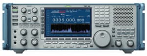


 Up to Contents
===========================================================================
V. PULSED MICROWAVE
Pulsed microwave voice-to-skull (or other-sound-to-skull) transmission
was discovered during World War II by radar technicians who found they
could hear the buzz of the train of pulses being transmitted by radar
equipment they were working on. This phenomenon has been studied
extensively by Dr. Allan Frey, whose work has been published in a number
of reference books.
What Dr. Frey found was that single pulses of microwave could be heard
by some people as "pops" or "clicks", while a train of uniform pulses
could be heard as a buzz, without benefit of any type of receiver.
Dr. Frey also found that a wide range of frequencies, as low as 125 MHz
(well below microwave) worked for some combination of pulse power and
pulse width. Detailed unclassified studies mapped out those frequencies
and pulse characteristics which are optimum for generation of "microwave
hearing".
Very significantly, when discussing electronic mind control, is the
fact that the PEAK PULSE POWER required is modest - something like
0.3 watts per square centimeter of skull surface, and this power level
is only applied for a very small percentage of each pulse's cycle time.
0.3 watts/sq cm is about what you get under a 250 watt heat lamp at
a distance of one meter. It is not a lot of power.
When you take into account that the pulse train is OFF (no signal) for
most of each cycle, the average power is so low as to be nearly
undetectable.
Frequencies that act as voice-to-skull carriers are not single freq-
uencies, as, for example TV or cell phone channels are. Each sensitive
frequency is actually a range or "band" of frequencies. A technology
used to reduce both interference and detection is called "spread
spectrum". Spread spectrum signals have the carrier frequency "hop"
around within a specified band.
Unless a receiver "knows" the hop schedule in advance, there is virtually
no chance of receiving or detecting a coherent readable signal. Spectrum
analyzers, used for detection, are receivers with a screen. A spread
spectrum signal received on a spectrum analyzer appears as just more
"static" or noise.
My organization was delighted to find the actual method of the first
successful UNclassified voice to skull experiment in 1974, by Dr.
Joseph C. Sharp, then at the Walter Reed Army Institute of Research.
Dr. Sharp's basic method is shown in Appendix PM6, below. A Frey-
type audible pulse was transmitted every time the voice waveform
passed down through the zero axis, a technique easily duplicated by
ham radio operators who build their own equipment.
A pattern seems to be repeated where research which could be used for
mind control starts working, the UNclassified researchers lose funding,
and in some cases their notes have been confiscated, and no further
information on that research track is heard in the unclassified press.
Pulsed microwave voice-to-skull research is one such track.
Up to Contents
===========================================================================
V. PULSED MICROWAVE
Pulsed microwave voice-to-skull (or other-sound-to-skull) transmission
was discovered during World War II by radar technicians who found they
could hear the buzz of the train of pulses being transmitted by radar
equipment they were working on. This phenomenon has been studied
extensively by Dr. Allan Frey, whose work has been published in a number
of reference books.
What Dr. Frey found was that single pulses of microwave could be heard
by some people as "pops" or "clicks", while a train of uniform pulses
could be heard as a buzz, without benefit of any type of receiver.
Dr. Frey also found that a wide range of frequencies, as low as 125 MHz
(well below microwave) worked for some combination of pulse power and
pulse width. Detailed unclassified studies mapped out those frequencies
and pulse characteristics which are optimum for generation of "microwave
hearing".
Very significantly, when discussing electronic mind control, is the
fact that the PEAK PULSE POWER required is modest - something like
0.3 watts per square centimeter of skull surface, and this power level
is only applied for a very small percentage of each pulse's cycle time.
0.3 watts/sq cm is about what you get under a 250 watt heat lamp at
a distance of one meter. It is not a lot of power.
When you take into account that the pulse train is OFF (no signal) for
most of each cycle, the average power is so low as to be nearly
undetectable.
Frequencies that act as voice-to-skull carriers are not single freq-
uencies, as, for example TV or cell phone channels are. Each sensitive
frequency is actually a range or "band" of frequencies. A technology
used to reduce both interference and detection is called "spread
spectrum". Spread spectrum signals have the carrier frequency "hop"
around within a specified band.
Unless a receiver "knows" the hop schedule in advance, there is virtually
no chance of receiving or detecting a coherent readable signal. Spectrum
analyzers, used for detection, are receivers with a screen. A spread
spectrum signal received on a spectrum analyzer appears as just more
"static" or noise.
My organization was delighted to find the actual method of the first
successful UNclassified voice to skull experiment in 1974, by Dr.
Joseph C. Sharp, then at the Walter Reed Army Institute of Research.
Dr. Sharp's basic method is shown in Appendix PM6, below. A Frey-
type audible pulse was transmitted every time the voice waveform
passed down through the zero axis, a technique easily duplicated by
ham radio operators who build their own equipment.
A pattern seems to be repeated where research which could be used for
mind control starts working, the UNclassified researchers lose funding,
and in some cases their notes have been confiscated, and no further
information on that research track is heard in the unclassified press.
Pulsed microwave voice-to-skull research is one such track.


Thanks for sharing
BalasHapusWaveguide mitter bends
Biofeedback equipment has many applications including stress management, pain management, and peak performance. When you decide that you want to make a purchase there are several things to consider.
BalasHapus