
X . I
Pulse generator
A pulse generator is either an electronic circuit or a piece of electronic test equipment used to generate rectangular pulses. Pulse generators are used primarily for working with digital circuits, related function generators are used primarily for analog circuits.
 Pulse generators in a physics laboratory
 Bench pulse generators
Simple bench pulse generators usually allow control of the pulse repetition rate (frequency), pulse width, delay with respect to an internal or external trigger and the high- and low-voltage levels of the pulses. More-sophisticated pulse generators may allow control over the rise time and fall time of the pulses. Pulse generators are available for generating output pulses having widths (duration) ranging from minutes down to under 1 picosecond. Pulse generators are generally voltage sources, with true current pulse generators being available only from a few suppliers. Pulse generators may use digital techniques, analog techniques, or a combination of both techniques to form the output pulses. For example, the pulse repetition rate and duration may be digitally controlled but the pulse amplitude and rise and fall times may be determined by analog circuitry in the output stage of the pulse generator. With correct adjustment, pulse generators can also produce a 50% duty cycle square wave. Pulse generators are generally single-channel providing one frequency, delay, width and output.Optical pulse generators
Light pulse generators are the optical equivalent to electrical pulse generators with rep rate, delay, width and amplitude control. The output in this case is light typically from a LED or laser diode.Multiple-channels
A new family of pulse generators can produce multiple-channels of independent widths and delays and independent outputs and polarities. Often called digital delay/pulse generators, the newest designs even offer differing repetition rates with each channel. These digital delay generators are useful in synchronizing, delaying, gating and triggering multiple devices usually with respect to one event. One is also able to multiplex the timing of several channels onto one channel in order to trigger or even gate the same device multiple times.A new class of pulse generator offers both multiple input trigger connections and multiple output connections. Multiple input triggers allows experimenters to synchronize both trigger events and data acquisition events using the same timing controller.
In general, generators for pulses with widths over a few microseconds employ digital counters for timing these pulses, while widths between approximately 1 nanosecond and several microseconds are typically generated by analog techniques such as RC (resistor-capacitor) networks or switched delay lines.
Microwave pulsers
Pulse generators capable of generating pulses with widths under approximately 100 picoseconds are often termed as "microwave pulsers" and typically generate these ultra-short pulses using Step recovery diode (SRD) or Nonlinear Transmission Line (NLTL) methods (for example ). Step Recovery Diode pulse generators are inexpensive but typically require several volts of input drive level and have a moderately high level of random jitter (usually undesirable variation in the time at which successive pulses occur).NLTL-based pulse generators generally have lower jitter, but are more complex to manufacture and do not suit integration in low-cost monolithic ICs. A new class of microwave pulse generation architecture, the RACE (Rapid Automatic Cascode Exchange) pulse generation circuit ,, is implemented using low-cost monolithic IC technology and can produce pulses as short as 1 picosecond, and with repetition rates exceeding 30 billion pulses per second. These pulsers are typically used in military communications applications, and low-power microwave transceiver ICs. Such pulsers, if driven by a continuous frequency clock, will act as microwave comb generators, having output frequency components at integer multiples of the pulse repetition rate, and extending to well over 100 gigahertz (for example ).
Applications
Pulses can then be injected into a device that is under test and used as a stimulus or clock signal or analyzed as they progress through the device, confirming the proper operation of the device or pinpointing a fault in the device. Pulse generators are also used to drive devices such as switches, lasers and optical components, modulators, intensifiers as well as resistive loads.The output of a pulse generator may also be used as the modulation signal for a signal generator. Non-electronic applications include those in material science, medical, physics and chemistry.Examples
- Ballistics testing uses high voltage pulse generator
- "Signal cable selection for Veritas Observatory" with <200 ps risetime pulse generator
- Single channel pulse generators were in existence in the 1950s
- "Characterization of Permalloy films on high-bandwidth striplines" Journal of Magnetism and Magnetic Materials Volumes 272-276, Supplement 1, May 2004, Pages E1341-E1342
- "Protoporphyrin IX Occurs Naturally in Colorectal Cancers and Their Metastases"
- Testing Silicon Strip Detector with IR Light Pulse Generator

 Tektronix 7854 oscilloscope with curve tracer and time-domain reflectometer plug-ins. Lower module has a digital voltmeter, a digital counter, an old WWVB frequency standard receiver with phase comparator, and function generator
 Test equipment switching
The addition of a high-speed switching system to a test system’s configuration allows for faster, more cost-effective testing of multiple devices, and is designed to reduce both test errors and costs. Designing a test system’s switching configuration requires an understanding of the signals to be switched and the tests to be performed, as well as the switching hardware form factors available.Types of test equipment
Basic equipment

Agilent commercial digital voltmeter checking a prototype
- Voltmeter (Measures voltage)
- Ohmmeter (Measures resistance)
- Ammeter, e.g. Galvanometer or Milliameter (Measures current)
- Multimeter e.g., VOM (Volt-Ohm-Milliammeter) or DMM (Digital Multimeter) (Measures all of the above)
- RLC Meter e.g., RLC meter or Resistance,Inductance and capacitance meter (measure RLC values)
The following analyze the response of the circuit under test:

- Oscilloscope (Displays voltage as it changes over time)
- Frequency counter (Measures frequency)
Advanced or less commonly used equipment
Meters- Solenoid voltmeter (Wiggy)
- Clamp meter (current transducer)
- Wheatstone bridge (Precisely measures resistance)
- Capacitance meter (Measures capacitance)
- LCR meter (Measures inductance, capacitance, resistance and combinations thereof)
- EMF Meter (Measures Electric and Magnetic Fields)
- Electrometer (Measures voltages, sometimes even tiny ones, via a charge effect)
Probes

Analyzers
- Logic analyzer (Tests digital circuits)
- Spectrum analyzer (SA) (Measures spectral energy of signals)
- Protocol analyzer (Tests functionality, performance and conformance of protocols)
- Vector signal analyzer (VSA) (Like the SA but it can also perform many more useful digital demodulation functions)
- Time-domain reflectometer (Tests integrity of long cables)
- Semiconductor curve tracer
Signal-generating devices

- Signal generator usually distinguished by frequency range (e.g., audio or radio frequencies) or waveform type (e.g., sine, square, sawtooth, ramp, sweep, modudulated, ...)
- Frequency synthesiser
- Function generator
- Digital pattern generator
- Pulse generator
- Signal injector
Miscellaneous devices
- Boxcar averager
- Continuity tester
- Cable tester
- Hipot tester
- Network analyzer (used to characterize an electrical network of components)
- Test light
- Transistor tester
- Tube tester
Platforms

Keithley Instruments Series 4200 CVU
GPIB/IEEE-488
The General Purpose Interface Bus (GPIB) is an IEEE-488 (a standard created by the Institute of Electrical and Electronics Engineers) standard parallel interface used for attaching sensors and programmable instruments to a computer. GPIB is a digital 8-bit parallel communications interface capable of achieving data transfers of more than 8 Mbytes/s. It allows daisy-chaining up to 14 instruments to a system controller using a 24-pin connector. It is one of the most common I/O interfaces present in instruments and is designed specifically for instrument control applications. The IEEE-488 specifications standardized this bus and defined its electrical, mechanical, and functional specifications, while also defining its basic software communication rules. GPIB works best for applications in industrial settings that require a rugged connection for instrument control.The original GPIB standard was developed in the late 1960s by Hewlett-Packard to connect and control the programmable instruments the company manufactured. The introduction of digital controllers and programmable test equipment created a need for a standard, high-speed interface for communication between instruments and controllers from various vendors. In 1975, the IEEE published ANSI/IEEE Standard 488-1975, IEEE Standard Digital Interface for Programmable Instrumentation, which contained the electrical, mechanical, and functional specifications of an interfacing system. This standard was subsequently revised in 1978 (IEEE-488.1) and 1990 (IEEE-488.2). The IEEE 488.2 specification includes the Standard Commands for Programmable Instrumentation (SCPI), which define specific commands that each instrument class must obey. SCPI ensures compatibility and configurability among these instruments.
The IEEE-488 bus has long been popular because it is simple to use and takes advantage of a large selection of programmable instruments and stimuli. Large systems, however, have the following limitations:
- Driver fanout capacity limits the system to 14 devices plus a controller.
- Cable length limits the controller-device distance to two meters per device or 20 meters total, whichever is less. This imposes transmission problems on systems spread out in a room or on systems that require remote measurements.
- Primary addresses limit the system to 30 devices with primary addresses. Modern instruments rarely use secondary addresses so this puts a 30-device limit on system size.
LAN eXtensions for Instrumentation
The LXI (LXI) Standard defines the communication protocols for instrumentation and data acquisition systems using Ethernet. These systems are based on small, modular instruments, using low-cost, open-standard LAN (Ethernet). LXI-compliant instruments offer the size and integration advantages of modular instruments without the cost and form factor constraints of card-cage architectures. Through the use of Ethernet communications, the LXI Standard allows for flexible packaging, high-speed I/O, and standardized use of LAN connectivity in a broad range of commercial, industrial, aerospace, and military applications. Every LXI-compliant instrument includes an Interchangeable Virtual Instrument (IVI) driver to simplify communication with non-LXI instruments, so LXI-compliant devices can communicate with devices that are not themselves LXI compliant (i.e., instruments that employ GPIB, VXI, PXI, etc.). This simplifies building and operating hybrid configurations of instruments.LXI instruments sometimes employ scripting using embedded test script processors for configuring test and measurement applications. Script-based instruments provide architectural flexibility, improved performance, and lower cost for many applications. Scripting enhances the benefits of LXI instruments, and LXI offers features that both enable and enhance scripting. Although the current LXI standards for instrumentation do not require that instruments be programmable or implement scripting, several features in the LXI specification anticipate programmable instruments and provide useful functionality that enhances scripting’s capabilities on LXI-compliant instruments.
VME eXtensions for Instrumentation
The VME eXtensions for Instrumentation (VXI) bus architecture is an open standard platform for automated test based on the VMEbus. Introduced in 1987, VXI uses all Eurocard form factors and adds trigger lines, a local bus, and other functions suited for measurement applications. VXI systems are based on a mainframe or chassis with up to 13 slots into which various VXI instrument modules can be installed.[3] The chassis also provides all the power supply and cooling requirements for the chassis and the instruments it contains. VXI bus modules are typically 6U in height.PCI eXtensions for Instrumentation
PCI eXtensions for Instrumentation, (PXI), is a peripheral bus specialized for data acquisition and real-time control systems. Introduced in 1997, PXI uses the CompactPCI 3U and 6U form factors and adds trigger lines, a local bus, and other functions suited for measurement applications. PXI hardware and software specifications are developed and maintained by the PXI Systems Alliance.[4] More than 50 manufacturers around the world produce PXI hardware.[5]Universal Serial Bus
The Universal Serial Bus (USB) connects peripheral devices, such as keyboards and mice, to PCs. The USB is a Plug and Play bus that can handle up to 127 devices on one port, and has a theoretical maximum throughput of 480 Mbit/s (high-speed USB defined by the USB 2.0 specification). Because USB ports are standard features of PCs, they are a natural evolution of conventional serial port technology. However, it is not widely used in building industrial test and measurement systems for several (e.g., USB cables are rarely industrial grade, are noise sensitive, are not positively attached and so are rather easily detachable, and the maximum distance between the controller and device is limited to a few meters). Like some other connections, USB is primarily used for applications in a laboratory setting that do not require a rugged bus connection.RS-232
RS-232 is a specification for serial communication that is popular in analytical and scientific instruments, as well for controlling peripherals such as printers. Unlike GPIB, with the RS-232 interface, it is possible to connect and control only one device at a time. RS-232 is also a relatively slow interface with typical data rates of less than 20 kbytes/s. RS-232 is best suited for laboratory applications compatible with a slower, less rugged connection.Test script processors and a channel expansion bus
One of the most recently developed test system platforms employs instrumentation equipped with onboard test script processors combined with a high-speed bus. In this approach, one “master” instrument runs a test script (a small program) that controls the operation of the various “slave” instruments in the test system, to which it is linked via a high-speed LAN-based trigger synchronization and inter-unit communication bus. Scripting is writing programs in a scripting language to coordinate a sequence of actions.This approach is optimized for small message transfers that are characteristic of test and measurement applications. With very little network overhead and a 100 Mbit/s data rate, it is significantly faster than GPIB and 100BaseT Ethernet in real applications.
The advantage of this platform is that all connected instruments behave as one tightly integrated multi-channel system, so users can scale their test system to fit their required channel counts cost-effectively. A system configured on this type of platform can stand alone as a complete measurement and automation solution, with the master unit controlling sourcing, measuring, pass/fail decisions, test sequence flow control, binning, and the component handler or prober. Support for dedicated trigger lines means that synchronous operations between multiple instruments equipped with onboard Test Script Processors that are linked by this high speed bus can be achieved without the need for additional trigger connections.
X . III
Network analyzer (electrical)
A network analyzer is an instrument that measures the network parameters of electrical networks. Today, network analyzers commonly measure s–parameters because reflection and transmission of electrical networks are easy to measure at high frequencies, but there are other network parameter sets such as y-parameters, z-parameters, and h-parameters. Network analyzers are often used to characterize two-port networks such as amplifiers and filters, but they can be used on networks with an arbitrary number of ports.
 ZVA40 vector network analyzer from Rohde & Schwarz.
 Network analyzers are used mostly at high frequencies; operating frequencies can range from 5 Hz to 1.05 THz.[1] Special types of network analyzers can also cover lower frequency ranges down to 1 Hz. These network analyzers can be used for example for the stability analysis of open loops or for the measurement of audio and ultrasonic components.[2]
The two basic types of network analyzers are
- scalar network analyzer (SNA)—measures amplitude properties only
- vector network analyzer (VNA)—measures both amplitude and phase properties
Another category of network analyzer is the microwave transition analyzer (MTA) or large signal network analyzer (LSNA), which measure both amplitude and phase of the fundamental and harmonics. The MTA was commercialized before the LSNA, but was lacking some of the user-friendly calibration features now available with the LSNA.
Architecture
The basic architecture of a network analyzer involves a signal generator, a test set, one or more receivers and display. In some setups, these units are distinct instruments. Most VNAs have two test ports, permitting measurement of four S-parameters (, , and ), but instruments with more than two ports are available commercially.


Signal generator
The network analyzer needs a test signal, and a signal generator or signal source will provide one. Older network analyzers did not have their own signal generator, but had the ability to control a stand-alone signal generator using, for example, a GPIB connection. Nearly all modern network analyzers have a built-in signal generator. High-performance network analyzers have two built-in sources. Two built-in sources are useful for applications such as mixer test, where one source provides the RF signal, another the LO, or amplifier intermodulation testing, where two tones are required for the test.Test set
The test set takes the signal generator output and routes it to the device under test, and it routes the signal to be measured to the receivers.It often splits off a reference channel for the incident wave. In a SNA, the reference channel may go to a diode detector (receiver) whose output is sent to the signal generator's automatic level control. The result is better control of the signal generator's output and better measurement accuracy. In a VNA, the reference channel goes to the receivers; it is needed to serve as a phase reference.Directional couplers or two resistor power dividers are used for signal separation. Some microwave test sets include the front end mixers for the receivers (e.g., test sets for HP 8510).
Receiver
The receivers make the measurements. A network analyzer will have one or more receivers connected to its test ports. The reference test port is usually labeled R, and the primary test ports are A, B, C,.... Some analyzers will dedicate a separate receiver to each test port, but others share one or two receivers among the ports. The R receiver may be less sensitive than the receivers used on the test ports.For the SNA, the receiver only measures the magnitude of the signal. A receiver can be a detector diode that operates at the test frequency. The simplest SNA will have a single test port, but more accurate measurements are made when a reference port is also used. The reference port will compensate for amplitude variations in the test signal at the measurement plane. It is possible to share a single detector and use it for both the reference port and the test port by making two measurement passes.
For the VNA, the receiver measures both the magnitude and the phase of the signal. It needs a reference channel (R) to determine the phase, so a VNA needs at least two receivers. The usual method down converts the reference and test channels to make the measurements at a lower frequency. The phase may be measured with a quadrature detector. A VNA requires at least two receivers, but some will have three or four receivers to permit simultaneous measurement of different parameters.
There are some VNA architectures (six-port) that infer phase and magnitude from just power measurements.
Processor and display
With the processed RF signal available from the receiver / detector section it is necessary to display the signal in a format that can be interpreted. With the levels of processing that are available today, some very sophisticated solutions are available in RF network analyzers. Here the reflection and transmission data is formatted to enable the information to be interpreted as easily as possible. Most RF network analyzers incorporate features including linear and logarithmic sweeps, linear and log formats, polar plots, Smith charts, etc. Trace markers, limit lines and also pass / fail criteria may also be added in many instances.[3]S-parameter measurement with vector network analyzer
A VNA is a test system that enables the RF performance of radio frequency and microwave devices to be characterised in terms of network scattering parameters, or S parameters.
The diagram shows the essential parts of a typical 2-port vector network analyzer (VNA). The two ports of the device under test (DUT) are denoted port 1 (P1) and port 2 (P2). The test port connectors provided on the VNA itself are precision types which will normally have to be extended and connected to P1 and P2 using precision cables 1 and 2, PC1 and PC2 respectively and suitable connector adaptors A1 and A2 respectively.
The test frequency is generated by a variable frequency CW source and its power level is set using a variable attenuator. The position of switch SW1 sets the direction that the test signal passes through the DUT. Initially consider that SW1 is at position 1 so that the test signal is incident on the DUT at P1 which is appropriate for measuring and . The test signal is fed by SW1 to the common port of splitter 1, one arm (the reference channel) feeding a reference receiver for P1 (RX REF1) and the other (the test channel) connecting to P1 via the directional coupler DC1, PC1 and A1. The third port of DC1 couples off the power reflected from P1 via A1 and PC1, then feeding it to test receiver 1 (RX TEST1). Similarly, signals leaving P2 pass via A2, PC2 and DC2 to RX TEST2. RX REF1, RX TEST1, RX REF2 and RXTEST2 are known as coherent receivers as they share the same reference oscillator, and they are capable of measuring the test signal's amplitude and phase at the test frequency. All of the complex receiver output signals are fed to a processor which does the mathematical processing and displays the chosen parameters and format on the phase and amplitude display. The instantaneous value of phase includes both the temporal and spatial parts, but the former is removed by virtue of using 2 test channels, one as a reference and the other for measurement. When SW1 is set to position 2, the test signals are applied to P2, the reference is measured by RX REF2, reflections from P2 are coupled off by DC2 and measured by RX TEST2 and signals leaving P1 are coupled off by DC1 and measured by RX TEST1. This position is appropriate for measuring and .
Calibration or error correction
A network analyzer, like most electronic instruments requires periodic calibration - typically this is performed once per year and is performed by the manufacturer or by a 3rd party in a calibration laboratory. When the instrument is calibrated, it will usually have a sticker fixed to the outside, stating the date it was calibrated and when the next calibration is due. A calibration certificate will be issued.A vector network analyzer achieves highly accurate measurements by correcting for the systematic errors in the instrument, the characteristics of cables, adapters and test fixtures. The process of error correction, although commonly just called calibration, is an entirely different process, and may be performed by an engineer several times in an hour. Sometimes it is called user-calibration, to indicate the difference from periodic calibration by a manufacturer.
A network analyzer has connectors on its front panel, but the measurements are seldom made at the front panel. Usually some test cables will connect from the front panel to the device under test (DUT). The length of those cables will introduce a time delay and corresponding phase shift (affecting VNA measurements); the cables will also introduce some attenuation (affecting SNA and VNA measurements). The same is true for cables and couplers inside the network analyzer. All these factors will change with temperature. Calibration usually involves measuring known standards and using those measurements to compensate for systematic errors, but there are methods which do not require known standards. Only systematic errors can be corrected. Random errors, such as connector repeatability can not be corrected by the user calibration. However, some portable vector network analyzers, designed for lower accuracy measurement outside using batteries, do attempt some correction for temperature by measuring the internal temperature of the network analyzer.
The first steps, prior to actually starting the user calibration are:
- Visually inspect the connectors for any problems such as bent pins or parts which are obviously off-centre. These should be thrown away, as mating damaged connectors with good connectors will often result in damaging the good connector.
- Clean the connectors with compressed air at less than 60 psi.
- If necessary clean the connectors with isopropyl alcohol.
- Gage the connectors to determine there are not any gross mechanical problems. Connector gauges with resolutions of 0.001" to 0.0001" will usually be included in the better quality calibration kits.
- Torque the connectors to the specified torque. A torque wrench will be supplied with all but the cheapest calibration kits.
- SOLT : which is an acronym for Short, Open, Load, Thru, is the simplest method. As the name suggests, this requires access to known standards with a short circuit, open circuit, a precision load (usually 50 ohms) and a through connection. It is best if the test ports have the same type of connector (N, 3,5 mm etc.), but of a different sex, so the through just requires the test ports are connected together. SOLT is suitable for coaxial measurements, where it is possible to obtain the short, open, load and through. The SOLT calibration method is less suitable for waveguide measurements, where it is difficult to obtain an open circuit or a load, or for measurements on non-coaxial test fixtures, where the same problems with finding suitable standards exist.
- TRL(through-reflect-line calibration): This technique is useful for microwave, noncoaxial environments such as fixture, wafer probing, or waveguide. TRL uses a transmission line, significantly longer in electrical length than the through line, of known length and impedance as one standard. TRL also requires a high-reflection standard (usually, a short or open) whose impedance does not have to be well characterized, but it must be electrically the same for both test ports.
- Directivity—error resulting from the portion of the source signal that never reaches the DUT.
- Source match—errors resulting from multiple internal reflections between the source and the DUT.
- Reflection tracking—error resulting from all frequency dependence of test leads, connections, etc.
A more complex calibration is a full 2-port reflectivity and transmission calibration. For two ports there are 12 possible systematic errors analogous to the three above. The most common method for correcting for these involves measuring a short, load and open standard on each of the two ports, as well as transmission between the two ports.
It is impossible to make a perfect short circuit, as there will always be some inductance in the short. It is impossible to make a perfect open circuit, as there will always be some fringing capacitance. A modern network analyzer will have data stored about the devices in a calibration kit. (Agilent 2006) For the open-circuit, this will be some electrical delay (typically tens of picoseconds), and fringing capacitance which will be frequency dependent. The capacitance is normally specified in terms of a polynomial, with the coefficients specific to each standard. A short will have some delay, and a frequency dependent inductance, although the inductance is normally considered insignificant below about 6 GHz. The definitions for a number of standards used in Agilent calibration kits can be found at http://na.tm.agilent.com/pna/caldefs/stddefs.html The definitions of the standards for a particular calibration kit will often change depending on the frequency range of the network analyzer. If a calibration kit works to 9 GHz, but a particular network analyzer has a maximum frequency of operation of 3 GHz, then the capacitance of the open standard can approximated more closely up to 3 GHz, using a different set of coefficients than are necessary to work up to 9 GHz.
In some calibration kits, the data on the males is different from the females, so the user needs to specify the sex of the connector. In other calibration kits (e.g. Agilent 85033E 9 GHz 3.5 mm), the male and female have identical characteristics, so there is no need for the user to specify the sex. For sexless connectors, like APC-7, this issues does not arise.
Most network analyzers will have the ability to have a user defined calibration kit. So if a user has a particular calibration kit, details of which are not in the firmware of the network analyzer, the data about the kit can be loaded into the network analyzer and so the kit used. Typically the calibration data can be entered on the instrument front panel, as well as loaded from a medium such as floppy disk or USB stick, or down a bus such as USB or GPIB.
The more expensive calibration kits will usually include a torque wrench to tighten connectors properly and a connector gauge to ensure there are no gross errors in the connectors.
Automated calibration fixtures
A calibration using a mechanical calibration kit may take a significant amount of time. Not only must the operator sweep through all the frequencies of interest, but the operator must also disconnect and reconnect the various standards. To avoid that work, network analyzers can employ automated calibration standards. The operator connects one box to the network analyzer. The box has a set of standards inside and some switches that have already been characterized. The network analyzer can read the characterization and control the configuration using a digital bus such as USB.Network analyzer verification kits
A number of verification kits are available to verify the network analyzer is performing to specification. These typically consist of transmission lines with an air dielectric and attenuators. The Agilent 85055A kit includes a 10 cm airline, stepped impedance airline, 20 dB and 50 dB attenuators with data on the devices measured by the manufacturer and stored on both a floppy disk and USB flash drive. Older versions of the 85055A have the data stored on tape and floppy disks rather than on USB drives.Noise figure measurements
The three major manufacturers of VNAs, Keysight, Anritsu, and Rohde & Schwarz, all produce models which permit the use of noise figure measurements. The vector error correction permits higher accuracy than is possible with other forms of commercial noise figure meters.X . IIII
SMITH CHART
The Smith chart, invented by Phillip H. Smith (1905–1987), is a graphical aid or nomogram designed for electrical and electronics engineers specializing in radio frequency (RF) engineering to assist in solving problems with transmission lines and matching circuits.[3] The Smith chart can be used to simultaneously display multiple parameters including impedances, admittances, reflection coefficients, scattering parameters, noise figure circles, constant gain contours and regions for unconditional stability, including mechanical vibrations analysis. The Smith chart is most frequently used at or within the unity radius region. However, the remainder is still mathematically relevant, being used, for example, in oscillator design and stability analysis.

Use of the Smith chart utility has grown steadily over the years and it is still widely used today, not only as a problem solving aid, but as a graphical demonstrator of how many RF parameters behave at one or more frequencies, an alternative to using tabular information.
 An impedance Smith chart (with no data plotted)
 The Smith chart is plotted on the complex reflection coefficient plane in two dimensions and is scaled in normalised impedance (the most common), normalised admittance or both, using different colours to distinguish between them. These are often known as the Z, Y and YZ Smith charts respectively.[7] Normalised scaling allows the Smith chart to be used for problems involving any characteristic or system impedance which is represented by the center point of the chart. The most commonly used normalization impedance is 50 ohms. Once an answer is obtained through the graphical constructions described below, it is straightforward to convert between normalised impedance (or normalised admittance) and the corresponding unnormalized value by multiplying by the characteristic impedance (admittance). Reflection coefficients can be read directly from the chart as they are unitless parameters.
The Smith chart has circumferential scaling in wavelengths and degrees. The wavelengths scale is used in distributed component problems and represents the distance measured along the transmission line connected between the generator or source and the load to the point under consideration. The degrees scale represents the angle of the voltage reflection coefficient at that point. The Smith chart may also be used for lumped element matching and analysis problems.
Use of the Smith chart and the interpretation of the results obtained using it requires a good understanding of AC circuit theory and transmission line theory, both of which are pre-requisites for RF engineers.
As impedances and admittances change with frequency, problems using the Smith chart can only be solved manually using one frequency at a time, the result being represented by a point. This is often adequate for narrow band applications (typically up to about 5% to 10% bandwidth) but for wider bandwidths it is usually necessary to apply Smith chart techniques at more than one frequency across the operating frequency band. Provided the frequencies are sufficiently close, the resulting Smith chart points may be joined by straight lines to create a locus.
A locus of points on a Smith chart covering a range of frequencies can be used to visually represent:
- how capacitive or how inductive a load is across the frequency range
- how difficult matching is likely to be at various frequencies
- how well matched a particular component is.
Mathematical basis

Most basic use of an impedance Smith chart. A wave travels down a transmission line of characteristic impedance Z0, terminated at a load with impedance ZL and normalised impedance z=ZL/Z0. There is a signal reflection with coefficient Γ. Each point on the Smith chart simultaneously represents both a value of z (bottom left), and the corresponding value of Γ (bottom right), related by z=(1+Γ)/(1-Γ).
Actual and normalised impedance and admittance
A transmission line with a characteristic impedance of may be universally considered to have a characteristic admittance of where


The normalised impedance Smith chart


- and


- is the temporal part of the wave
- is the spatial part of the wave and
- where
- is the angular frequency in radians per second (rad/s)
- is the frequency in hertz (Hz)
- is the time in seconds (s)
- and are constants
- is the distance measured along the transmission line from the load toward the generator in metres (m)


- is the propagation constant which has units 1/m

- is the attenuation constant in nepers per metre (Np/m)
- is the phase constant in radians per metre (rad/m)


- and


The variation of complex reflection coefficient with position along the line

Looking towards a load through a length l of lossless transmission line, the impedance changes as l increases, following the blue circle. (This impedance is characterized by its reflection coefficient Vreflected / Vincident.) The blue circle, centered within the impedance Smith chart, is sometimes called an SWR circle (short for constant standing wave ratio).


For a uniform transmission line (in which is constant), the complex reflection coefficient of a standing wave varies according to the position on the line. If the line is lossy ( is non-zero) this is represented on the Smith chart by a spiral path. In most Smith chart problems however, losses can be assumed negligible () and the task of solving them is greatly simplified. For the loss free case therefore, the expression for complex reflection coefficient becomes


Therefore

The variation of normalised impedance with position along the line
If and are the voltage across and the current entering the termination at the end of the transmission line respectively, then

- and
- .


- .


Both and are expressed in complex numbers without any units. They both change with frequency so for any particular measurement, the frequency at which it was performed must be stated together with the characteristic impedance.
may be expressed in magnitude and angle on a polar diagram. Any actual reflection coefficient must have a magnitude of less than or equal to unity so, at the test frequency, this may be expressed by a point inside a circle of unity radius. The Smith chart is actually constructed on such a polar diagram. The Smith chart scaling is designed in such a way that reflection coefficient can be converted to normalised impedance or vice versa. Using the Smith chart, the normalised impedance may be obtained with appreciable accuracy by plotting the point representing the reflection coefficient treating the Smith chart as a polar diagram and then reading its value directly using the characteristic Smith chart scaling. This technique is a graphical alternative to substituting the values in the equations.
By substituting the expression for how reflection coefficient changes along an unmatched loss free transmission line

- .


Versions of the transmission line equation may be similarly derived for the admittance loss free case and for the impedance and admittance lossy cases.
The Smith chart graphical equivalent of using the transmission line equation is to normalise , to plot the resulting point on a Z Smith chart and to draw a circle through that point centred at the Smith chart centre. The path along the arc of the circle represents how the impedance changes whilst moving along the transmission line. In this case the circumferential (wavelength) scaling must be used, remembering that this is the wavelength within the transmission line and may differ from the free space wavelength.
Regions of the Z Smith chart
If a polar diagram is mapped on to a cartesian coordinate system it is conventional to measure angles relative to the positive x-axis using a counterclockwise direction for positive angles. The magnitude of a complex number is the length of a straight line drawn from the origin to the point representing it. The Smith chart uses the same convention, noting that, in the normalised impedance plane, the positive x-axis extends from the center of the Smith chart at to the point . The region above the x-axis represents inductive impedances (positive imaginary parts) and the region below the x-axis represents capacitive impedances (negative imaginary parts).

If the termination is perfectly matched, the reflection coefficient will be zero, represented effectively by a circle of zero radius or in fact a point at the centre of the Smith chart. If the termination was a perfect open circuit or short circuit the magnitude of the reflection coefficient would be unity, all power would be reflected and the point would lie at some point on the unity circumference circle.
Circles of constant normalised resistance and constant normalised reactance
The normalised impedance Smith chart is composed of two families of circles: circles of constant normalised resistance and circles of constant normalised reactance. In the complex reflection coefficient plane the Smith chart occupies a circle of unity radius centred at the origin. In cartesian coordinates therefore the circle would pass through the points (1,0) and (-1,0) on the x-axis and the points (0,1) and (0,-1) on the y-axis.Since both and are complex numbers, in general they may be written as:


Substituting these into the equation relating normalised impedance and complex reflection coefficient:

- .

The Y Smith chart
The Y Smith chart is constructed in a similar way to the Z Smith chart case but by expressing values of voltage reflection coefficient in terms of normalised admittance instead of normalised impedance. The normalised admittance yT is the reciprocal of the normalised impedance zT, so


The region above the x-axis represents capacitive admittances and the region below the x-axis represents inductive admittances. Capacitive admittances have positive imaginary parts and inductive admittances have negative imaginary parts.
Again, if the termination is perfectly matched the reflection coefficient will be zero, represented by a 'circle' of zero radius or in fact a point at the centre of the Smith chart. If the termination was a perfect open or short circuit the magnitude of the voltage reflection coefficient would be unity, all power would be reflected and the point would lie at some point on the unity circumference circle of the Smith chart.
Practical examples
A point with a reflection coefficient magnitude 0.63 and angle 60° represented in polar form as , is shown as point P1 on the Smith chart. To plot this, one may use the circumferential (reflection coefficient) angle scale to find the graduation and a ruler to draw a line passing through this and the centre of the Smith chart. The length of the line would then be scaled to P1 assuming the Smith chart radius to be unity. For example if the actual radius measured from the paper was 100 mm, the length OP1 would be 63 mm.


The following table gives some similar examples of points which are plotted on the Z Smith chart. For each, the reflection coefficient is given in polar form together with the corresponding normalised impedance in rectangular form. The conversion may be read directly from the Smith chart or by substitution into the equation.
| Point Identity | Reflection Coefficient (Polar Form) | Normalised Impedance (Rectangular Form) |
|---|---|---|
| P1 (Inductive) | ||
| P2 (Inductive) | ||
| P3 (Capacitive) |


Working with both the Z Smith chart and the Y Smith charts
In RF circuit and matching problems sometimes it is more convenient to work with admittances (representing conductances and susceptances) and sometimes it is more convenient to work with impedances (representing resistances and reactances). Solving a typical matching problem will often require several changes between both types of Smith chart, using normalised impedance for series elements and normalised admittances for parallel elements. For these a dual (normalised) impedance and admittance Smith chart may be used. Alternatively, one type may be used and the scaling converted to the other when required. In order to change from normalised impedance to normalised admittance or vice versa, the point representing the value of reflection coefficient under consideration is moved through exactly 180 degrees at the same radius. For example the point P1 in the example representing a reflection coefficient of has a normalised impedance of . To graphically change this to the equivalent normalised admittance point, say Q1, a line is drawn with a ruler from P1 through the Smith chart centre to Q1, an equal radius in the opposite direction. This is equivalent to moving the point through a circular path of exactly 180 degrees. Reading the value from the Smith chart for Q1, remembering that the scaling is now in normalised admittance, gives . Performing the calculation

Once a transformation from impedance to admittance has been performed the scaling changes to normalised admittance until such time that a later transformation back to normalised impedance is performed.
The table below shows examples of normalised impedances and their equivalent normalised admittances obtained by rotation of the point through 180°. Again these may either be obtained by calculation or using a Smith chart as shown, converting between the normalised impedance and normalised admittances planes.
| Normalised Impedance Plane | Normalised Admittance Plane |
|---|---|
| P1 () | Q1 () |
| P10 () | Q10 () |


Choice of Smith chart type and component type
The choice of whether to use the Z Smith chart or the Y Smith chart for any particular calculation depends on which is more convenient. Impedances in series and admittances in parallel add while impedances in parallel and admittances in series are related by a reciprocal equation. If is the equivalent impedance of series impedances and is the equivalent impedance of parallel impedances, then


| Element Type | Impedance (Z or z) or Reactance (X or x) | Admittance (Y or y) or Susceptance (B or b) | ||
|---|---|---|---|---|
| Real () | Normalised (No Unit) | Real (S) | Normalised (No Unit) | |
| Resistance (R) | ||||
| Inductance (L) | ||||
| Capacitance (C) | ||||


Using the Smith chart to solve conjugate matching problems with distributed components
Usually distributed matching is only feasible at microwave frequencies since, for most components operating at these frequencies, appreciable transmission line dimensions are available in terms of wavelengths. Also the electrical behavior of many lumped components becomes rather unpredictable at these frequencies.For distributed components the effects on reflection coefficient and impedance of moving along the transmission line must be allowed for using the outer circumferential scale of the Smith chart which is calibrated in wavelengths.
The following example shows how a transmission line, terminated with an arbitrary load, may be matched at one frequency either with a series or parallel reactive component in each case connected at precise positions.
Supposing a loss-free air-spaced transmission line of characteristic impedance , operating at a frequency of 800 MHz, is terminated with a circuit comprising a 17.5 resistor in series with a 6.5 nanohenry (6.5 nH) inductor. How may the line be matched?


From the table above, the reactance of the inductor forming part of the termination at 800 MHz is


- .


The conjugate match for the impedance at P21 () is


- .


An alternative shunt match could be calculated after performing a Smith chart transformation from normalised impedance to normalised admittance. Point Q20 is the equivalent of P20 but expressed as a normalised admittance. Reading from the Smith chart scaling, remembering that this is now a normalised admittance gives


- .


The conjugate matching component is required to have a normalised admittance () of

- .


Using the Smith chart to analyze lumped element circuits
The analysis of lumped element components assumes that the wavelength at the frequency of operation is much greater than the dimensions of the components themselves. The Smith chart may be used to analyze such circuits in which case the movements around the chart are generated by the (normalized) impedances and admittances of the components at the frequency of operation. In this case the wavelength scaling on the Smith chart circumference is not used. The following circuit will be analyzed using a Smith chart at an operating frequency of 100 MHz. At this frequency the free space wavelength is 3 m. The component dimensions themselves will be in the order of millimetres so the assumption of lumped components will be valid. Despite there being no transmission line as such, a system impedance must still be defined to enable normalization and de-normalization calculations and is a good choice here as . If there were very different values of resistance present a value closer to these might be a better choice.

The analysis starts with a Z Smith chart looking into R1 only with no other components present. As is the same as the system impedance, this is represented by a point at the centre of the Smith chart. The first transformation is OP1 along the line of constant normalized resistance in this case the addition of a normalized reactance of -j0.80, corresponding to a series capacitor of 40 pF. Points with suffix P are in the Z plane and points with suffix Q are in the Y plane. Therefore transformations P1 to Q1 and P3 to Q3 are from the Z Smith chart to the Y Smith chart and transformation Q2 to P2 is from the Y Smith chart to the Z Smith chart. The following table shows the steps taken to work through the remaining components and transformations, returning eventually back to the centre of the Smith chart and a perfect 50 ohm match.


| Transformation | Plane | x or y Normalized Value | Capacitance/Inductance | Formula to Solve | Result |
|---|---|---|---|---|---|
| Capacitance (Series) | |||||
| Inductance (Shunt) | |||||
| Z | Capacitance (Series) | ||||
| Y | Capacitance (Shunt) |


3D Smith chart
A generalized 3D Smith chart based on the extended complex plane (Riemann sphere) and inversive geometry was proposed in 2011. The chart unifies the passive and active circuit design on little and big circles on the surface of a unit sphere using the stereographic conformal map of the reflection coefficient's generalized plane. Considering the point at infinity, the space of the new chart includes all possible loads. The north pole is the perfect matching point, while the south pole is the perfect mismatch point.
X . IIIII
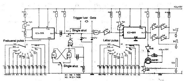
Example of a pulse generator on the motion of the vehicle's speed
TCI Modern ignition
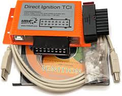
Now let's go to a more modern ignition like Platina instead of CDI, that is DC-TCI (digitally controlled transistorized coil ignition system) a clear understanding of sparks that have the duration ..... DC-TCI can be found in the ignition system Yamaha Vixion and some other similar bikapa like Thunder 125 and Ninja 250
This system controls ignition timing with a microkomputer (ecu) located within the spark unit and calculates the ideal ignition timing at all engine speeds. This mechanism has a safety that will cut the power line to the Ignition Coil when the ignition time has an abnormality.
The Control Unit consists of:• One Distributor• the receiver, which processes the pulse signal from the pulse generator• a microcomputer, which has memory and a calculating unit
The rotor that generates the pulse has some kind of protrusion (reluctor) placed at an irregular distance. Whenever this reluctor passes through the pulse generator, a pulse will be sent to the spark unit. The number and angle between the different relays depends on the number of cylinders and their placement. The diagram below is for the 90 "v-twin ignition system.

Ignition steps:
1. After the engine is turned on, a pulse signal is sent from the pulse generator to the spark unit.
2. The receiver unit converts the pulse signal into a digital signal that is inserted into the microcomputer.
3. Once the digital signal received microcomputer, it also processes the angle of the crankshaft and engine speed. Then the microcomputer reads the information about the ignition timing, which is in memory, then determines how many timings are right. Then the microcomputer sends current to the base foot of the transistor.
4. By flowing the base current from the microcomputer to the transistor, the transistor turns on and acts as an electronic switch that ignites the spark plug.
Quick note:
Basically ignition with this system is the same principle, just take advantage of electronic technology as its main parts, namely microcomputers, transistors, and signal receivers ..
With the addition of microcomputers, the ignition timing can be programmed memories (mapping), and the presence of transistors can respond to the commands more quickly.

X . IIIIIII
Pulse (interbank network)
Pulse is an interbank electronic funds transfer (EFT) network in the United States. It serves more than 4,400 U.S. financial institutions and includes more than 380,000 ATMs, as well as POS terminals nationwide. Rivals of the network include First Data's STAR and Fidelity National Information Services's NYCE. It is owned by Discover Financial, issuer of the Discover Card, and is included in Discover's agreement with China UnionPay; cards can be used on each other's network leading to better acceptance outside large cities than the larger networks.
The Pulse system was based on the A O Smith software that operated the Take Your Money Everywhere (TYME) network operating in the northern plains states. The network was established as the banking rules that limited banks and branches ability to share services were removed. The data processing facilities were originally provided by First City Bank and later transitioned to Texas Commerce Bank.
- 1995, Pulse launches Pulse Pay, a point-of-sale service where cardholders can use their ATM card at retailers.
- 1997, Pulse announced acquisition of Gulfnet, the Louisiana-based regional EFT network.
- 2000, Pulse announced it would acquire the Cincinnati-based MoneyStation network.
- 2002, Pulse merged with Wisconsin-based Tyme Corporation.
- 2005, Pulse is acquired by the Discover Financial Services
- Currently, Pulse is a California Residential Mortgage Licensee (License Number MLS-18827).
Automated teller machine
An automated teller machine, also known in the United States of America as an automatic teller machine[1][2][3] (ATM, American, British, Australian, Malaysian, South African, Singaporean, Indian, Maldivian, Hiberno, Philippine and Sri Lankan English), automated banking machine (ABM, Canadian English[4]), cash point (British English[5]), cashline, minibank, cash machine, cash dispenser, bankomat or bancomat is an electronic telecommunications device that enables the customers of a financial institution to perform financial transactions, particularly cash withdrawal, without the need for a human cashier, clerk or bank teller.According to the ATM Industry Association (ATMIA),[6] there are now close to 3.5 million ATMs installed worldwide.[7]
On most modern ATMs, the customer is identified by inserting a plastic ATM card with a magnetic stripe or a plastic smart card with a chip that contains a unique card number and some security information such as an expiration date or CVVC (CVV). Authentication is provided by the customer entering a personal identification number (PIN) which must match the PIN stored in the chip on the card (if the card is so equipped) or in the issuing financial institution's database.
Using an ATM, customers can access their bank deposit or credit accounts in order to make a variety of transactions such as cash withdrawals, check balances, or credit mobile phones. If the currency being withdrawn from the ATM is different from that in which the bank account is denominated the money will be converted at an official exchange rate. Thus, ATMs often provide the best possible exchange rates for foreign travellers, and are widely used for this purpose.[8]

Most ATMs are connected to interbank networks, enabling people to withdraw and deposit money from machines not belonging to the bank where they have their accounts or in the countries where their accounts are held (enabling cash withdrawals in local currency). Some examples of interbank networks include NYCE, PULSE, PLUS, Cirrus, AFFN, Interac, Interswitch, STAR, LINK, MegaLink and BancNet.
ATMs rely on authorization of a financial transaction by the card issuer or other authorizing institution on a communications network. This is often performed through an ISO 8583 messaging system.
Many banks charge ATM usage fees. In some cases, these fees are charged solely to users who are not customers of the bank where the ATM is installed; in other cases, they apply to all users.
In order to allow a more diverse range of devices to attach to
.
Customer identity integrity
There have also been a number of incidents of fraud by Man-in-the-middle attacks, where criminals have attached fake keypads or card readers to existing machines. These have then been used to record customers' PINs and bank card information in order to gain unauthorised access to their accounts. Various ATM manufacturers have put in place countermeasures to protect the equipment they manufacture from these threats.[68][69]
Alternative methods to verify cardholder identities have been tested and deployed in some countries, such as finger and palm vein patterns,[70] iris, and facial recognition technologies. Cheaper mass-produced equipment has been developed and is being installed in machines global
 ly that detect the presence of foreign objects on the front of ATMs, current tests have shown 99% detection success for all types of skimming devices.[71]

Uses
 Two NCR Personas 84 ATMs at a bank in Jersey dispensing two types of pound sterling banknotes: Bank of England on the left, and States of Jersey on the right.
 Gold vending ATM in New York City.
Originally developed as cash dispensers, ATMs have evolved to include many other bank-related functions:
Gold vending ATM in New York City.
Originally developed as cash dispensers, ATMs have evolved to include many other bank-related functions:
- Paying routine bills, fees, and taxes (utilities, phone bills, social security, legal fees, income taxes, etc.)
- Printing bank statements
- Updating passbooks
- Cash advances
- Cheque Processing Module
- Paying (in full or partially) the credit balance on a card linked to a specific current account.
- Transferring money between linked accounts (such as transferring between accounts)
- Deposit currency recognition, acceptance, and recycling[85][86]
In some countries, especially those which benefit from a fully integrated cross-bank network (e.g.: Multibanco in Portugal), ATMs include many functions that are not directly related to the management of one's own bank account, such as:
- Loading monetary value into stored value cards
- Adding pre-paid cell phone / mobile phone credit.
- Purchasing
- Concert tickets
- Gold[87]
- Lottery tickets
- Movie tickets
- Postage stamps.
- Train tickets
- Shopping mall gift certificates.
- Donating to charities[88]
Increasingly, banks are seeking to use the ATM as a sales device to deliver pre approved loans and targeted advertising using products such as ITM (the Intelligent Teller Machine) from Aptra Relate from NCR.[89] ATMs can also act as an advertising channel for other companies.[90]*
 However, several different ATM technologies have not yet reached worldwide acceptance, such as:
- Videoconferencing with human tellers, known as video tellers[91]
- Biometrics, where authorization of transactions is based on the scanning of a customer's fingerprint, iris, face, etc.[92][93][94]
- Cheque/cash Acceptance, where the machine accepts and recognises cheques and/or currency without using envelopes[95] Expected to grow in importance in the US through Check 21 legislation.
- Bar code scanning[96]
- On-demand printing of "items of value" (such as movie tickets, traveler's cheques, etc.)
- Dispensing additional media (such as phone cards)
- Co-ordination of ATMs with mobile phones[97]
- Integration with non-banking equipment[98][99]
- Games and promotional features[100]
- CRM through the ATM
In Canada, ATMs are called guichets automatiques in French and sometimes "bank machines" in English. The Interac-shared cash network does not allow for the selling of goods from ATMs, due to specific security requirements for PIN entry when buying goods.[101] CIBC machines in Canada, are able to top-up the minutes on certain pay as you go phones.

Two NCR Personas 84 ATMs at a bank in Jersey dispensing two types of pound sterling banknotes: Bank of England on the left, and States of Jersey on the right.

Gold vending ATM in New York City.
- Concert tickets
- Gold[87]
- Lottery tickets
- Movie tickets
- Postage stamps.
- Train tickets
- Shopping mall gift certificates.

Reliability
 Before an ATM is placed in a public place, it typically has undergone extensive testing with both test money and the backend computer systems that allow it to perform transactions. Banking customers also have come to expect high reliability in their ATMs,[102] which provides incentives to ATM providers to minimise machine and network failures. Financial consequences of incorrect machine operation also provide high degrees of incentive to minimise malfunctions.[103]
ATMs and the supporting electronic financial networks are generally very reliable, with industry benchmarks typically producing 98.25% customer availability for ATMs[104] and up to 99.999% availability for host systems that manage the networks of ATMs. If ATM networks do go out of service, customers could be left without the ability to make transactions until the beginning of their bank's next time of opening hours.
This said, not all errors are to the detriment of customers; there have been cases of machines giving out money without debiting the account, or giving out higher value notes as a result of incorrect denomination of banknote being loaded in the money cassettes.[105] The result of receiving too much money may be influenced by the card holder agreement in place between the customer and the bank.[106][107]
Errors that can occur may be mechanical (such as card transport mechanisms; keypads; hard disk failures; envelope deposit mechanisms); software (such as operating system; device driver; application); communications; or purely down to operator error.
To aid in reliability, some ATMs print each transaction to a roll-paper journal that is stored inside the ATM, which allows its users and the related financial institutions to settle things based on the records in the journal in case there is a dispute. In some cases, transactions are posted to an electronic journal to remove the cost of supplying journal paper to the ATM and for more convenient searching of data.
Improper money checking can cause the possibility of a customer receiving counterfeit banknotes from an ATM. While bank personnel are generally trained better at spotting and removing counterfeit cash,[108][109] the resulting ATM money supplies used by banks provide no guarantee for proper banknotes, as the Federal Criminal Police Office of Germany has confirmed that there are regularly incidents of false banknotes having been dispensed through ATMs.[110] Some ATMs may be stocked and wholly owned by outside companies, which can further complicate this problem. Bill validation technology can be used by ATM providers to help ensure the authenticity of the cash before it is stocked in the machine; those with cash recycling capabilities include this capability.

Electronic funds transfer
Electronic funds transfer (EFT) is the electronic transfer of money from one bank account to another, either within a single financial institution or across multiple institutions, via computer-based systems, without the direct intervention of bank staff. EFT's are known by a number of names. In the United States, they may be referred to as electronic checks or e-checks.
The term covers a number of different payment systems, for example:
- cardholder-initiated transactions, using a payment card such as a credit or debit card
- direct deposit payment initiated by the payer
- direct debit payments for which a business debits the consumer's bank accounts for payment for goods or services
- wire transfer via an international banking network such as SWIFT
- electronic bill payment in online banking, which may be delivered by EFT or paper check
- transactions involving stored value of electronic money, possibly in a private currency.
Digital currency
Digital currency or digital money or electronic money is distinct from physical (such as banknotes and coins). It exhibits properties similar to physical currencies, but allows for instantaneous transactions and borderless transfer-of-ownership. Examples include virtual currencies and cryptocurrencies.[1] Like traditional money, these currencies may be used to buy physical goods and services, but may also be restricted to certain communities such as for use inside an on-line game or social ne
Digital versus virtual currency
According to the European Central Bank's "Virtual currency schemes – a further analysis" report of February 2015, virtual currency is a digital representation of value, not issued by a central bank, credit institution or e-money institution, which, in some circumstances, can be used as an alternative to money. In the previous report of October 2012, the virtual currency was defined as a type of unregulated, digital money, which is issued and usually controlled by its developers, and used and accepted among the members of a specific virtual community.According to the Bank For International Settlements' "Digital currencies" report of November 2015, digital currency is an asset represented in digital form and having some monetary characteristics. Digital currency can be denominated to a sovereign currency and issued by the issuer responsible to redeem digital money for cash. In that case, digital currency represents electronic money (e-money). Digital currency denominated in its own units of value or with decentralized or automatic issuance will be considered as a virtual currency.
As such, bitcoin is a digital currency but also a type of virtual currency. Bitcoin and its alternatives are based on cryptographic algorithms, so these kinds of virtual currencies are also called cryptocurrencies.
Digital versus traditional currency
Most of the traditional money supply is bank money held on computers. This is also considered digital currency. One could argue that our increasingly cashless society means that all currencies are becoming digital (sometimes referred to as “electronic money”), but they are not presented to us as such.[12]Types of systems
Centralized systems
Many systems—such as PayPal, eCash, WebMoney, Payoneer, cashU, and Hub Culture's Ven will sell their electronic currency [clarification needed] directly to the end user. Other systems only sell through third party digital currency exchangers. The M-Pesa system is used to transfer money through mobile phones in Africa, India, Afghanistan, and Eastern Europe. Some community currencies, like some local exchange trading systems (LETS) and the Community Exchange System, work with electronic transactions.Mobile digital wallets[edit]
A number of electronic money systems use contactless payment transfer in order to facilitate easy payment and give the payee more confidence in not letting go of their electronic wallet during the transaction.- In 1994 Mondex and National Westminster Bank provided an 'electronic purse' to residents of Swindon
- In about 2005 Telefónica and BBVA Bank launched a payment system in Spain called Mobipay[13] which used simple short message service facilities of feature phones intended for pay-as you go services including taxis and pre-pay phone recharges via a BBVA current bank account debit.
- In Jan 2010, Venmo launched as a mobile payment system through SMS, which transformed into a social app where friends can pay each other for minor expenses like a cup of coffee, rent and paying your share of the restaurant bill when you forget your wallet.[14] It is popular with college students, but has some security issues.[15] It can be linked to your bank account, credit/debit card or have a loaded value to limit the amount of loss in case of a security breach. Credit cards and non-major debit cards incur a 3% processing fee.[16]
- On September 19, 2011, Google Wallet was released in the US only, which makes it easy to carry all your credit/debit cards on your phone.[17]
- In 2012 O2 (Ireland) (owned by Telefónica) launched Easytrip[18] to pay road tolls which were charged to the mobile phone account or prepay credit.
- O2 (United Kingdom) invented O2 Wallet[19] at about the same time. The wallet can be charged with regular bank accounts or cards and discharged by participating retailers using a technique known as 'money messages' The service closed in 2014
- On September 9, 2014 Apple Pay was announced at the iPhone 6 event. In October 2014 it was released as an update to work on iPhone 6 and Apple Watch. It is very similar to Google Wallet, but for Apple devices only.[20]
- GNU Taler is an anonymous, open source electronic payment system in development.
Decentralized systems
Unofficial bitcoin logo
In some cases a proof-of-work scheme is used to create and manage the currency.
Cryptocurrencies allow electronic money systems to be decentralized; systems include:
- Bitcoin, a peer-to-peer electronic monetary system based on cryptography.
- Litecoin, originally based on the bitcoin protocol, intended to improve upon its alleged inefficiencies.
- Ripple monetary system, a monetary system based on trust networks.
- Dogecoin, a Litecoin-derived system meant by its author to reach broader demographics.
- Nxt, conceived as flexible platform to build applications and financial services around.
- Monero, an open source cryptocurrency created in April 2014 that focuses on privacy, decentralisation and scalability.
Virtual currency
Virtual currency
A virtual currency has been defined in 2012 by the European Central Bank as "a type of unregulated, digital money, which is issued and usually controlled by its developers, and used and accepted among the members of a specific virtual community". The US Department of Treasury in 2013 defined it more tersely as "a medium of exchange that operates like a currency in some environments, but does not have all the attributes of real currency". The key attribute a virtual currency does not have according to these definitions, is the status as legal tender.Law
Since 2001, the European Union has implemented the E-Money Directive "on the taking up, pursuit and prudential supervision of the business of electronic money institutions" last amended in 2009.[25] Doubts on the real nature of EU electronic money have arisen, since calls have been made in connection with the 2007 EU Payment Services Directive in favor of merging payment institutions and electronic money institutions. Such a merger could mean that electronic money is of the same nature as bank money or scriptural money.In the United States, electronic money is governed by Article 4A of the Uniform Commercial Code for wholesale transactions and the Electronic Fund Transfer Act for consumer transactions. Provider's responsibility and consumer's liability are regulated under Regulation E.[26][27]
Regulation
Virtual currencies pose challenges for central banks, financial regulators, departments or ministries of finance, as well as fiscal authorities and statistical authorities.US Treasury guidance
On 20 March 2013, the Financial Crimes Enforcement Network issued a guidance to clarify how the US Bank Secrecy Act applied to persons creating, exchanging and transmitting virtual currencies.[28]Securities and Exchange Commission guidance
In May 2014 the U.S. Securities and Exchange Commission (SEC) "warned about the hazards of bitcoin and other virtual currencies".[29]New York state regulation
In July 2014, the New York State Department of Financial Services proposed the most comprehensive regulation of virtual currencies to date, commonly called BitLicense.[30] Unlike the US federal regulators it has gathered input from bitcoin supporters and the financial industry through public hearings and a comment period until 21 October 2014 to customize the rules. The proposal per NY DFS press release “... sought to strike an appropriate balance that helps protect consumers and root out illegal activity".[31] It has been criticized by smaller companies to favor established institutions, and Chinese bitcoin exchanges have complained that the rules are "overly broad in its application outside the United States".[32]Adoption by governments
As of 2016, over 24 countries are investing in distributed ledger technologies (DLT) with $1.4bn in investments. In addition, over 90 central banks are engaged in DLT discussions, including implications of a central bank issued digital currency.[33]- Hong Kong’s Octopus card system: Launched in 1997 as an electronic purse for public transportation, is the most successful and mature implementation of contactless smart cards used for mass transit payments. After only 5 years, 25 percent of Octopus card transactions are unrelated to transit, and accepted by more than 160 merchants.[34]
- London Transport’s Oyster card system: Oyster is a plastic smartcard which can hold pay as you go credit, Travelcards and Bus & Tram season tickets. You can use an Oyster card to travel on bus, Tube, tram, DLR, London Overground and most National Rail services in London.[35]
- Japan’s FeliCa: A contactless RFID smart card, used in a variety of ways such as in ticketing systems for public transportation, e-money, and residence door keys.[36]
- Netherlands’ Chipknip: As an electronic cash system used in the Netherlands, all ATM cards issued by the Dutch banks had value that could be loaded via Chipknip loading stations. For people without a bank, pre-paid Chipknip cards could be purchased at various locations in the Netherlands. As of January 1, 2015, you can no longer pay with Chipknip.[37]
- Belgium’s Proton: An electronic purse application for debit cards in Belgium. Introduced in February 1995, as a means to replace cash for small transactions. The system was retired in December 31, 2014.[38]
- Canada
The Bank of Canada teamed up with the nation’s five largest banks — and the blockchain consulting firm R3 — for what was known as Project Jasper. In a simulation run in 2016, the central bank issued CAD-Coins onto a blockchain similar Ethereum.[40] The banks used the CAD-Coins to exchange money the way they do at the end of each day to settle their master accounts.[40]
- China
- Denmark
- Ecuador
- Germany
- Netherlands
- Russia
- South Korea
- Sweden
- Switzerland
Swiss Federal Railways, government-owned railway company of Switzerland, sells bitcoins at its ticket machines.[54][54]
- UK
The chief economist of Bank of England, the central bank of the United Kingdom, proposed abolition of paper currency. The Bank has also taken an interest in bitcoin.[40][56] In 2016 it has embarked on a multi-year research programme to explore the implications of a central bank issued digital currency.[33] The Bank of England has produced several research papers on the topic. One suggests that the economic benefits of issuing a digital currency on a distributed ledger could add as much as 3 percent to a country’s economic output.[40] The Bank said that it wanted the next version of the bank’s basic software infrastructure to be compatible with distributed ledgers.[40]
- Ukraine
Hard vs. soft digital currencies
A hard electronic currency is one that does not have services to dispute or reverse charges. In other words, it is akin to cash in that it only supports non-reversible transactions. Reversing transactions, even in case of a legitimate error, unauthorized use, or failure of a vendor to supply goods is difficult, if not impossible. The advantage of this arrangement is that the operating costs of the electronic currency system are greatly reduced by not having to resolve payment disputes. Additionally, it allows the electronic currency transactions to clear instantly, making the funds available immediately to the recipient. This means that using hard electronic currency is more akin to a cash transaction. Examples are Western Union, KlickEx and Bitcoin.A soft electronic currency is one that allows for reversal of payments, for example in case of fraud or disputes. Reversible payment methods generally have a "clearing time" of 72 hours or more. Examples are PayPal and credit card. A hard currency can be softened by using a trusted third party or an escrow service.
Criticism
Many of existing digital currencies have not yet seen widespread usage, and may not be easily used or exchanged. Banks generally do not accept or offer services for them.[58] There are concerns that cryptocurrencies are extremely risky due to their very high volatility[59] and potential for pump and dump schemes.[60] Regulators in several countries have warned against their use and some have taken concrete regulatory measures to dissuade users.[61] The non-cryptocurrencies are all centralized. As such, they may be shut down or seized by a government at any time.[62] The more anonymous a currency is, the more attractive it is to criminals, regardless of the intentions of its creators.[62] Forbes writer Tim Worstall has written that the value of bitcoin is largely derived from speculative trading.[63] Bitcoin has also been criticised for its energy inefficient SHA-256-based proof of work.[64]twork.[2]Digital currency is a money balance recorded electronically on a stored-value card or other device. Another form of electronic money is network money, allowing the transfer of value on computer networks, particularly the Internet. Electronic money is also a claim on a private bank or other financial institution such as bank deposits.[3]
Digital money can either be centralized, where there is a central point of control over the money supply, or decentralized, where the control over the money supply can come from various sources.

Tidak ada komentar:
Posting Komentar