Electronically Defined Natural Attributes (eDNA) ; not AND in logic i ( R,L,C trans )

Internet security start-up Oxford Bio-Chronometrics developed Electronically Defined Natural Attributes (eDNA) which blocks spam bots and makes the Internet easier for humans.
e-DNA is more unique than a fingerprint or a retina scan since it’s the result of hundreds of different behaviors measured continuously while a user interacts with any kind digital content – a website, ad, login, registration form or contact form. While bots, hackers and scammers can perhaps mimic a few of these behaviors, nothing is able to replicate them all.
About 500 different behaviors are unique to every individual and, taken together, form what they call ‘eDNA’ continue to this discovery researchers from University of Oxford says that they can also detect when a person is drunk or has had sex.
Over a period of time automated programs are great hazards for webmasters. CEO for the Bio-Chronometrics says “Forcing humans to enter a code they can barely read makes many of them go away, now the new R&D could allow our physical behavior to be used as a secure way of logging in to our computers and smart phones.
eDNA would be able to locate whether a click on an advertisement or a site is from an automated program, or so-called bot, or a real human. “We can hold companies like Google and Facebook to account ,and they know this technology is coming .
How your electronic DNA could be the secure login of the future
Unique habits can be used to prove users' identity – but may also reveal if they are drunk, or have had sex, researchers say

About 500 different behaviours are unique to every individual and, taken together, form what they call ‘eDNA’
New research could allow our physical behaviour to be used as a secure way of logging in to our computers and smartphones, a team at the University of Oxford say, claiming that they can also detect when a person is drunk or has had sex.
Researchers have identified that every individual creates a unique pattern of physical behaviour including the speed at which they type, the way they move a mouse of the way they hold a phone.
About 500 different behaviours are unique to every individual and, taken together, form what they call "eDNA", or electronically Defined Natural Attributes. Changes in this string of physical behaviour might even be able to signal when someone has taken drugs, had sex, or if they might be susceptible to a heart attack in three months’ time.
"Electronic DNA allows us to see vastly more information about you, who developed the technology while studying for an MSc at the university and is now chief executive of Oxford BioChronometrics.
"Like DNA it is almost impossible to fake, as it is very hard to go online and not be yourself. It is as huge a jump in the amount of information that could be gathered about an individual as the jump from fingerprints to DNA. It is that order of magnitude."
Oxford BioChronometrics is a startup from Oxford University that with the help of Isis Innovation Software Incubator is being transferred into the private sector, or spun out, on 18 July in order to take the commercialisation of the technology to the next stage. Isis Innovation is the technology transfer company of Oxford University. Biochronometrics is the measurement of change in biological behaviour over time.
"It is easy to tell when someone has been taking drugs using this technology," says Neal. "But it would place us in a difficult situation if we did. So it’s best we don’t. We just want to collect the data to make sure that x is who x says they are."
Oxford BioChronometrics, says that eDNA would be able to spot whether a click on an advert or a site is from an automated program, or so-called bot, or a real human. "We can hold companies like Google and Facebook to account ,and they know this technology is coming," he said.
Oxford BioChronometrics' own research suggests that 90-92% of clicks on adverts and 95% of logins are actually from bots. Their first product NoMoreCaptchas which stops spam bots from registering and logging on has already quietly been rolled out to 700 companies.
Adrian Neal, a former cryptographic expert, said the eDNA project has its roots in several decades' worth of research including biometrics, which can measure keystrokes or mouse movements, but these were thought to be too insecure to use as a login principle.
As computing power, along with the ability to gather large volumes of information from users, researchers were able to identify much broader and more complex patterns of interaction with their devices.
Information Security Group at Royal Holloway, is more sceptical that eDNA will reach the mainstream. "Using different factors to prove your identity online is always good," he says, but believes consumers won't be happy to be continuously assessed in this way. "It may also add to the cost and inconvenience of business as companies’ own software will likely have to be rejigged."
"But there will also be resistance by customers if you find your behaviour monitored, a little bit of pushback
Researchers Can Identify You From The Way You Type And Use Your Mouse

New research could allow our physical behaviour to be used as a secure way of logging in to our computers and smartphones, a team at the University of Oxford say, claiming that they can also detect when a person is drunk or has had sex.
Researchers have identified that every individual creates a unique pattern of physical behaviour including the speed at which they type, the way they move a mouse of the way they hold a phone.
About 500 different behaviours are unique to every individual and, taken together, form what they call "eDNA", or electronically Defined Natural Attributes. Changes in this string of physical behaviour might even be able to signal when someone has taken drugs, had sex, or if they might be susceptible to a heart attack in three months’ time.

e-DNA User Authentication distinguishes bots from humans and humans from each other based on hundreds of behavioral data points users don’t even notice they make. We let in who and what you want, and keep the rest away based on the digital signature created by the user’s behavior.
We call this identifier the user’s Electronically Defined Natural Attributes, or e-DNA and it is the new proof-positive of user identification and authentication.
Typical biometrics require multiple different angles/captures of a physical attribute to attain a high degree of confidence.
Behavioral biometrics relies on collecting enough behavioral data from different “angles” (time, activity, sensory data, etc.) to produce a confidence level that the user is who they claim to be. Thanks to the high level of complexity of understanding and mapping behavior, e-DNA User Authentication is highly secure with many added benefits .
How It Works
Behavioral data is acquired via a collection script embedded in the webpage or app the user is visiting. The script relays as many data points as possible from a given device to servers which perform the analysis.
There are no additional steps/challenges to complete because the collection code and back-end processing are invisible to the user.
There are no additional steps/challenges to complete because the collection code and back-end processing are invisible to the user.

A Good Solution Gets Better with Time The way we measure behavior, certainty improves with increased use. The more user-device interaction/behavioral data collected, the more effective the e-DNA becomes.
Behavior is the Key, Not Hardware or Puzzles
By scrutinizing real-time behavior, e-DNA User Authentication can determine if a user is permitted to access something without ever breaching their (or your) privacy.

X . I Signal
A signal as referred to in communication systems, signal processing, and electrical engineering is a function that "conveys information about the behavior or attributes of some phenomenon". In the physical world, any quantity exhibiting variation in time or variation in space (such as an image) is potentially a signal that might provide information on the status of a physical system, or convey a message between observers, among other possibilities. The IEEE Transactions on Signal Processing states that the term "signal" includes audio, video, speech, image, communication, geophysical, sonar, radar, medical and musical signals.
In nature, signals can take the form of any action by one organism able to be perceived by other organisms, ranging from the release of chemicals by plants to alert nearby plants of the same type of a predator, to sounds or motions made by animals to alert other animals of the presence of danger or of food. Signaling occurs in organisms all the way down to the cellular level, with cell signaling. Signaling theory, in evolutionary biology, proposes that a substantial driver for evolution is the ability for animals to communicate with each other by developing ways of signaling. In human engineering, signals are typically provided by a sensor, and often the original form of a signal is converted to another form of energy using a transducer. For example, a microphone converts an acoustic signal to a voltage waveform, and a speaker does the reverse.
The formal study of the information content of signals is the field of information theory. The information in a signal is usually accompanied by noise. The term noise usually means an undesirable random disturbance, but is often extended to include unwanted signals conflicting with the desired signal (such as crosstalk). The prevention of noise is covered in part under the heading of signal integrity. The separation of desired signals from a background is the field of signal recovery,[4] one branch of which is estimation theory, a probabilistic approach to suppressing random disturbances.
Engineering disciplines such as electrical engineering have led the way in the design, study, and implementation of systems involving transmission, storage, and manipulation of information. In the latter half of the 20th century, electrical engineering itself separated into several disciplines, specialising in the design and analysis of systems that manipulate physical signals; electronic engineering and computer engineering as examples; while design engineering developed to deal with functional design of man–machine interfaces .

In "The Signal" painting by William Powell Frith, a woman waves a handkerchief as a signal to a person able to see this action, in order to convey a message to this person .
Definitions
Definitions specific to sub-fields are common. For example, in information theory, a signal is a codified message, that is, the sequence of states in a communication channel that encodes a message.In the context of signal processing, arbitrary binary data streams are not considered as signals, but only analog and digital signals that are representations of analog physical quantities.
In a communication system, a transmitter encodes a message to a signal, which is carried to a receiver by the communications channel. For example, the words "Mary had a little lamb" might be the message spoken into a telephone. The telephone transmitter converts the sounds into an electrical voltage signal. The signal is transmitted to the receiving telephone by wires; at the receiver it is reconverted into sounds.
In telephone networks, signalling, for example common-channel signaling, refers to phone number and other digital control information rather than the actual voice signal.
Signals can be categorized in various ways. The most common distinction is between discrete and continuous spaces that the functions are defined over, for example discrete and continuous time domains. Discrete-time signals are often referred to as time series in other fields. Continuous-time signals are often referred to as continuous signals even when the signal functions are not continuous; an example is a square-wave signal.
A second important distinction is between discrete-valued and continuous-valued. Particularly in digital signal processing a digital signal is sometimes defined as a sequence of discrete values, that may or may not be derived from an underlying continuous-valued physical process. In other contexts, digital signals are defined as the continuous-time waveform signals in a digital system, representing a bit-stream. In the first case, a signal that is generated by means of a digital modulation method is considered as converted to an analog signal, while it is considered as a digital signal in the second case.
Another important property of a signal (actually, of a statistically defined class of signals) is its entropy or information content.
Analog and digital signals
Analog signal
An analog signal is any continuous signal for which the time varying feature (variable) of the signal is a representation of some other time varying quantity, i.e., analogous to another time varying signal. For example, in an analog audio signal, the instantaneous voltage of the signal varies continuously with the pressure of the sound waves. It differs from a digital signal, in which the continuous quantity is a representation of a sequence of discrete values which can only take on one of a finite number of values. The term analog signal usually refers to electrical signals; however, mechanical, pneumatic, hydraulic, human speech, and other systems may also convey or be considered analog signals.An analog signal uses some property of the medium to convey the signal's information. For example, an aneroid barometer uses rotary position as the signal to convey pressure information. In an electrical signal, the voltage, current, or frequency of the signal may be varied to represent the information.
Any information may be conveyed by an analog signal; often such a signal is a measured response to changes in physical phenomena, such as sound, light, temperature, position, or pressure. The physical variable is converted to an analog signal by a transducer. For example, in sound recording, fluctuations in air pressure (that is to say, sound) strike the diaphragm of a microphone which induces corresponding fluctuations in the current produced by a coil in an electromagnetic microphone, or the voltage produced by a condenser microphone. The voltage or the current is said to be an "analog" of the sound.
Digital signal
A digital signal is a signal that is constructed from a discrete set of waveforms of a physical quantity so as to represent a sequence of discrete values. A logic signal is a digital signal with only two possible values,[10][11] and describes an arbitrary bit stream. Other types of digital signals can represent three-valued logic or higher valued logics.Alternatively, a digital signal may be considered to be the sequence of codes represented by such a physical quantity.[12] The physical quantity may be a variable electric current or voltage, the intensity, phase or polarization of an optical or other electromagnetic field, acoustic pressure, the magnetization of a magnetic storage media, etcetera. Digital signals are present in all digital electronics, notably computing equipment and data transmission.

A received digital signal may be impaired by noise and distortions without necessarily affecting the digits
Digital signals often arise via sampling of analog signals, for example, a continually fluctuating voltage on a line that can be digitized by an analog-to-digital converter circuit, wherein the circuit will read the voltage level on the line, say, every 50 microseconds and represent each reading with a fixed number of bits. The resulting stream of numbers is stored as digital data on a discrete-time and quantized-amplitude signal. Computers and other digital devices are restricted to discrete time.
Time discretization

Discrete-time signal created from a continuous signal by sampling
If for a signal, the quantities are defined only on a discrete set of times, we call it a discrete-time signal. A simple source for a discrete time signal is the sampling of a continuous signal, approximating the signal by a sequence of its values at particular time instants.
A discrete-time real (or complex) signal can be seen as a function from (a subset of) the set of integers (the index labeling time instants) to the set of real (or complex) numbers (the function values at those instants).
A continuous-time real (or complex) signal is any real-valued (or complex-valued) function which is defined at every time t in an interval, most commonly an infinite interval.
Amplitude quantization

Examples of signals
Signals in nature can be converted to electronic signals by various sensors. Some examples are:- Motion. The motion of an object can be considered to be a signal, and can be monitored by various sensors to provide electrical signals. For example, radar can provide an electromagnetic signal for following aircraft motion. A motion signal is one-dimensional (time), and the range is generally three-dimensional. Position is thus a 3-vector signal; position and orientation of a rigid body is a 6-vector signal. Orientation signals can be generated using a gyroscope.
- Sound. Since a sound is a vibration of a medium (such as air), a sound signal associates a pressure value to every value of time and three space coordinates. A sound signal is converted to an electrical signal by a microphone, generating a voltage signal as an analog of the sound signal, making the sound signal available for further signal processing. Sound signals can be sampled at a discrete set of time points; for example, compact discs (CDs) contain discrete signals representing sound, recorded at 44,100 samples per second; each sample contains data for a left and right channel, which may be considered to be a 2-vector signal (since CDs are recorded in stereo). The CD encoding is converted to an electrical signal by reading the information with a laser, converting the sound signal to an optical signal.[15]
- Images. A picture or image consists of a brightness or color signal, a function of a two-dimensional location. The object's appearance is presented as an emitted or reflected electromagnetic wave, one form of electronic signal. It can be converted to voltage or current waveforms using devices such as the charge-coupled device. A 2D image can have a continuous spatial domain, as in a traditional photograph or painting; or the image can be discretized in space, as in a raster scanned digital image. Color images are typically represented as a combination of images in three primary colors, so that the signal is vector-valued with dimension three.
- Videos. A video signal is a sequence of images. A point in a video is identified by its two-dimensional position and by the time at which it occurs, so a video signal has a three-dimensional domain. Analog video has one continuous domain dimension (across a scan line) and two discrete dimensions (frame and line).
- Biological membrane potentials. The value of the signal is an electric potential ("voltage"). The domain is more difficult to establish. Some cells or organelles have the same membrane potential throughout; neurons generally have different potentials at different points. These signals have very low energies, but are enough to make nervous systems work; they can be measured in aggregate by the techniques of electrophysiology.
Signal processing
A typical role for signals is in signal processing. A common example is signal transmission between different locations. The embodiment of a signal in electrical form is made by a transducer that converts the signal from its original form to a waveform expressed as a current (I) or a voltage (V), or an electromagnetic waveform, for example, an optical signal or radio transmission. Once expressed as an electronic signal, the signal is available for further processing by electrical devices such as electronic amplifiers and electronic filters, and can be transmitted to a remote location by electronic transmitters and received using electronic receivers.
Signals and systems
The field studies input and output signals, and the mathematical representations between them known as systems, in four domains: Time, Frequency, s and z. Since signals and systems are both studied in these four domains, there are 8 major divisions of study. As an example, when working with continuous time signals (t), one might transform from the time domain to a frequency or s domain; or from discrete time (n) to frequency or z domains. Systems also can be transformed between these domains like signals, with continuous to s and discrete to z.
Although S and S falls under and includes all the topics covered in this article, as well as Analog signal processing and Digital signal processing, it actually is a subset of the field of Mathematical modeling. The field goes back to RF over a century ago, when it was all analog, and generally continuous. Today, software has taken the place of much of the analog circuitry design and analysis, and even continuous signals are now generally processed digitally. Ironically, digital signals also are processed continuously in a sense, with the software doing calculations between discrete signal "rests" to prepare for the next input/transform/output event.
In past EE curricula S and S, as it is often called, involved circuit analysis and design via mathematical modeling and some numerical methods, and was updated several decades ago with Dynamical systems tools including differential equations, and recently, Lagrangians. The difficulty of the field at that time included the fact that not only mathematical modeling, circuits, signals and complex systems were being modeled, but physics as well, and a deep knowledge of electrical (and now electronic) topics also was involved and required.
Today, the field has become even more daunting and complex with the addition of circuit, systems and signal analysis and design languages and software, from MATLAB and Simulink to NumPy, VHDL, PSpice, Verilog and even Assembly language. Students are expected to understand the tools as well as the mathematics, physics, circuit analysis, and transformations between the 8 domains.
Because mechanical engineering topics like friction, dampening etc. have very close analogies in signal science (inductance, resistance, voltage, etc.), many of the tools originally used in ME transformations (Laplace and Fourier transforms, Lagrangians, sampling theory, probability, difference equations, etc.) have now been applied to signals, circuits, systems and their components, analysis and design in EE. Dynamical systems that involve noise, filtering and other random or chaotic attractors and repellors have now placed stochastic sciences and statistics between the more deterministic discrete and continuous functions in the field. (Deterministic as used here means signals that are completely determined as functions of time).
EE taxonomists are still not decided where S&S falls within the whole field of signal processing vs. circuit analysis and mathematical modeling, but the common link of the topics that are covered in the course of study has brightened boundaries with dozens of books, journals, etc. called Signals and Systems, and used as text and test prep for the EE, as well as, recently, computer engineering exams. The Hsu general reference given below is a good example, with a new edition scheduled for late 2013/ early 2014.
X . II
Digital image processing
Digital image processing is the use of computer algorithms to perform image processing on digital images. As a subcategory or field of digital signal processing, digital image processing has many advantages over analog image processing. It allows a much wider range of algorithms to be applied to the input data and can avoid problems such as the build-up of noise and signal distortion during processing. Since images are defined over two dimensions (perhaps more) digital image processing may be modeled in the form of multidimensional systems.
Many of the techniques of digital image processing, or digital picture processing as it often was called, were developed in the 1960s at the Jet Propulsion Laboratory, Massachusetts Institute of Technology, Bell Laboratories, University of Maryland, and a few other research facilities, with application to satellite imagery, wire-photo standards conversion, medical imaging, videophone, character recognition, and photograph enhancement.[1] The cost of processing was fairly high, however, with the computing equipment of that era. That changed in the 1970s, when digital image processing proliferated as cheaper computers and dedicated hardware became available. Images then could be processed in real time, for some dedicated problems such as television standards conversion. As general-purpose computers became faster, they started to take over the role of dedicated hardware for all but the most specialized and computer-intensive operations. With the fast computers and signal processors available in the 2000s, digital image processing has become the most common form of image processing and generally, is used because it is not only the most versatile method, but also the cheapest.
Digital image processing technology for medical applications was inducted into the Space Foundation Space Technology Hall of Fame in 1994.
In 2002 Raanan Fattel, introduced Gradient domain image processing, a new way to process images in which the differences between pixels are manipulated rather than the pixel values themselves.
Tasks
Digital image processing allows the use of much more complex algorithms, and hence, can offer both more sophisticated performance at simple tasks, and the implementation of methods which would be impossible by analog means.In particular, digital image processing is the only practical technology for:
Some techniques which are used in digital image processing include:
- Anisotropic diffusion
- Hidden Markov models
- Image editing
- Image restoration
- Independent component analysis
- Linear filtering
- Neural networks
- Partial differential equations
- Pixelation
- Principal components analysis
- Self-organizing maps
- Wavelets
Digital image transformations
Filtering
Digital filters are used to blur and sharpen digital images. Filtering can be performed in the spatial domain by convolution with specifically designed kernels (filter array), or in the frequency (Fourier) domain by masking specific frequency regions. The following examples show both methods:| Filter type | Kernel or mask | Example |
|---|---|---|
| Original Image |  | |
| Spatial Lowpass |  | |
| Spatial Highpass |  | |
| Fourier Representation | Pseudo-code: image = checkerboard F = Fourier Transform of image Show Image: log(1+Absolute Value(F)) |  |
| Fourier Lowpass |  |  |
| Fourier Highpass |  |  |


Image padding in Fourier domain filtering
Images are typically padded before being transformed to the Fourier space, the highpass filtered images below illustrate the consequences of different padding techniques:| Zero padded | Repeated edge padded |
|---|---|
|  |
Filtering Code Examples
MATLAB example for spatial domain highpass filtering.img=checkerboard(20); % generate checkerboard
% ************************** SPATIAL DOMAIN ***************************
klaplace=[0 -1 0; -1 5 -1; 0 -1 0]; % Laplacian filter kernel
X=conv2(img,klaplace); % convolve test img with
% 3x3 Laplacian kernel
figure()
imshow(X,[]) % show Laplacian filtered
title('Laplacian Edge Detection')
img=checkerboard(20);                           % generate checkerboard
% **************************  FOURIER DOMAIN  ***************************
pad=paddedsize([m,n]);                          % get padding size
imgp=padarray(img,[pad(1),pad(2)],'both');      % set pad before & after
[p,q]=size(imgp);                               % get size of padded img
fftpad=fft2(imgp);                              % Fourier transform
F=fftshift(fftpad);                             % shift low freq to middle

Hlp=fftshift(lpfilter('btw',p,q,60));           % get butterworth filter
Hhp=1-Hlp;                                      % get highpass
HPimg=abs(ifft2(F.*Hhp));                       % apply filter and IFFT
figure(7)
imshow(Hhp,[])                                  % show the filter
title('Highpass Butterworth')
figure(8)                                       % show result cropped
imshow(HPimg(round((p-n)/2):round(n+(p-n)/2),round((q-m)/2):round(m+(q-m)/2)),[])
title('FFT Highpass Filtered')
Affine transformations
Affine transformations enable basic image transformations including scale, rotate, translate, mirror and sheer as is shown in the following examples show:| Transformation Name | Affine Matrix | Example |
|---|---|---|
| Identity | | |
| Reflection |  | |
| Scale |  | |
| Rotate |  | |
| Shear |  |


Applications
Digital camera images
Digital cameras generally include specialized digital image processing hardware – either dedicated chips or added circuitry on other chips – to convert the raw data from their image sensor into a color-corrected image in a standard image file formatX . III
Computer vision
Computer vision is an interdisciplinary field that deals with how computers can be made for gaining high-level understanding from digital images or videos. From the perspective of engineering, it seeks to automate tasks that the human visual system can do.
Computer vision tasks include methods for acquiring, processing, analyzing and understanding digital images, and extraction of high-dimensional data from the real world in order to produce numerical or symbolic information, e.g., in the forms of decisions.[4][5][6][7] Understanding in this context means the transformation of visual images (the input of the retina) into descriptions of the world that can interface with other thought processes and elicit appropriate action. This image understanding can be seen as the disentangling of symbolic information from image data using models constructed with the aid of geometry, physics, statistics, and learning theory.[8]
As a scientific discipline, computer vision is concerned with the theory behind artificial systems that extract information from images. The image data can take many forms, such as video sequences, views from multiple cameras, or multi-dimensional data from a medical scanner. As a technological discipline, computer vision seeks to apply its theories and models for the construction of computer vision systems.
Sub-domains of computer vision include scene reconstruction, event detection, video tracking, object recognition, object pose estimation, learning, indexing, motion estimation, and image restoration.
Definition
Computer vision is an interdisciplinary field that deals with how computers can be made for gaining high-level understanding from digital images or videos. From the perspective of engineering, it seeks to automate tasks that the human visual system can do. "Computer vision is concerned with the automatic extraction, analysis and understanding of useful information from a single image or a sequence of images. It involves the development of a theoretical and algorithmic basis to achieve automatic visual understanding." [9] As a scientific discipline, computer vision is concerned with the theory behind artificial systems that extract information from images. The image data can take many forms, such as video sequences, views from multiple cameras, or multi-dimensional data from a medical scanner. As a technological discipline, computer vision seeks to apply its theories and models for the construction of computer vision systems.In the late 1960s, computer vision began at universities that were pioneering artificial intelligence. It was meant to mimic the human visual system, as a stepping stone to endowing robots with intelligent behavior. In 1966, it was believed that this could be achieved through a summer project, by attaching a camera to a computer and having it "describe what it saw".
What distinguished computer vision from the prevalent field of digital image processing at that time was a desire to extract three-dimensional structure from images with the goal of achieving full scene understanding. Studies in the 1970s formed the early foundations for many of the computer vision algorithms that exist today, including extraction of edges from images, labeling of lines, non-polyhedral and polyhedral modeling, representation of objects as interconnections of smaller structures, optical flow, and motion estimation.
The next decade saw studies based on more rigorous mathematical analysis and quantitative aspects of computer vision. These include the concept of scale-space, the inference of shape from various cues such as shading, texture and focus, and contour models known as snakes. Researchers also realized that many of these mathematical concepts could be treated within the same optimization framework as regularization and Markov random fields. By the 1990s, some of the previous research topics became more active than the others. Research in projective 3-D reconstructions led to better understanding of camera calibration. With the advent of optimization methods for camera calibration, it was realized that a lot of the ideas were already explored in bundle adjustment theory from the field of photogrammetry. This led to methods for sparse 3-D reconstructions of scenes from multiple images. Progress was made on the dense stereo correspondence problem and further multi-view stereo techniques. At the same time, variations of graph cut were used to solve image segmentation. This decade also marked the first time statistical learning techniques were used in practice to recognize faces in images (see Eigenface). Toward the end of the 1990s, a significant change came about with the increased interaction between the fields of computer graphics and computer vision. This included image-based rendering, image morphing, view interpolation, panoramic image stitching and early light-field rendering.
Recent work has seen the resurgence of feature-based methods, used in conjunction with machine learning techniques and complex optimization frameworks
Related fields
Areas of artificial intelligence deal with autonomous planning or deliberation for robotical systems to navigate through an environment. A detailed understanding of these environments is required to navigate through them. Information about the environment could be provided by a computer vision system, acting as a vision sensor and providing high-level information about the environment and the robot.Artificial intelligence and computer vision share other topics such as pattern recognition and learning techniques. Consequently, computer vision is sometimes seen as a part of the artificial intelligence field or the computer science field in general.
Solid-state physics is another field that is closely related to computer vision. Most computer vision systems rely on image sensors, which detect electromagnetic radiation, which is typically in the form of either visible or infra-red light. The sensors are designed using quantum physics. The process by which light interacts with surfaces is explained using physics. Physics explains the behavior of optics which are a core part of most imaging systems. Sophisticated image sensors even require quantum mechanics to provide a complete understanding of the image formation process. Also, various measurement problems in physics can be addressed using computer vision, for example motion in fluids.
A third field which plays an important role is neurobiology, specifically the study of the biological vision system. Over the last century, there has been an extensive study of eyes, neurons, and the brain structures devoted to processing of visual stimuli in both humans and various animals. This has led to a coarse, yet complicated, description of how "real" vision systems operate in order to solve certain vision related tasks. These results have led to a subfield within computer vision where artificial systems are designed to mimic the processing and behavior of biological systems, at different levels of complexity. Also, some of the learning-based methods developed within computer vision (e.g. neural net and deep learning based image and feature analysis and classification) have their background in biology.
Some strands of computer vision research are closely related to the study of biological vision – indeed, just as many strands of AI research are closely tied with research into human consciousness, and the use of stored knowledge to interpret, integrate and utilize visual information. The field of biological vision studies and models the physiological processes behind visual perception in humans and other animals. Computer vision, on the other hand, studies and describes the processes implemented in software and hardware behind artificial vision systems. Interdisciplinary exchange between biological and computer vision has proven fruitful for both fields.
Yet another field related to computer vision is signal processing. Many methods for processing of one-variable signals, typically temporal signals, can be extended in a natural way to processing of two-variable signals or multi-variable signals in computer vision. However, because of the specific nature of images there are many methods developed within computer vision which have no counterpart in processing of one-variable signals. Together with the multi-dimensionality of the signal, this defines a subfield in signal processing as a part of computer vision.
Beside the above-mentioned views on computer vision, many of the related research topics can also be studied from a purely mathematical point of view. For example, many methods in computer vision are based on statistics, optimization or geometry. Finally, a significant part of the field is devoted to the implementation aspect of computer vision; how existing methods can be realized in various combinations of software and hardware, or how these methods can be modified in order to gain processing speed without losing too much performance.
The fields most closely related to computer vision are image processing, image analysis and machine vision. There is a significant overlap in the range of techniques and applications that these cover. This implies that the basic techniques that are used and developed in these fields are similar, something which can be interpreted as there is only one field with different names. On the other hand, it appears to be necessary for research groups, scientific journals, conferences and companies to present or market themselves as belonging specifically to one of these fields and, hence, various characterizations which distinguish each of the fields from the others have been presented.
Computer graphics produces image data from 3D models, computer vision often produces 3D models from image data. There is also a trend towards a combination of the two disciplines, e.g., as explored in augmented reality.
The following characterizations appear relevant but should not be taken as universally accepted:
- Image processing and image analysis tend to focus on 2D images, how to transform one image to another, e.g., by pixel-wise operations such as contrast enhancement, local operations such as edge extraction or noise removal, or geometrical transformations such as rotating the image. This characterization implies that image processing/analysis neither require assumptions nor produce interpretations about the image content.
- Computer vision includes 3D analysis from 2D images. This analyzes the 3D scene projected onto one or several images, e.g., how to reconstruct structure or other information about the 3D scene from one or several images. Computer vision often relies on more or less complex assumptions about the scene depicted in an image.
- Machine vision is the process of applying a range of technologies & methods to provide imaging-based automatic inspection, process control and robot guidance[16] in industrial applications.[17] Machine vision tends to focus on applications, mainly in manufacturing, e.g., vision based robots and systems for vision based inspection or measurement. This implies that image sensor technologies and control theory often are integrated with the processing of image data to control a robot and that real-time processing is emphasised by means of efficient implementations in hardware and software. It also implies that the external conditions such as lighting can be and are often more controlled in machine vision than they are in general computer vision, which can enable the use of different algorithms.
- There is also a field called imaging which primarily focus on the process of producing images, but sometimes also deals with processing and analysis of images. For example, medical imaging includes substantial work on the analysis of image data in medical applications.
- Finally, pattern recognition is a field which uses various methods to extract information from signals in general, mainly based on statistical approaches and artificial neural networks. A significant part of this field is devoted to applying these methods to image data.
Applications
Applications range from tasks such as industrial machine vision systems which, say, inspect bottles speeding by on a production line, to research into artificial intelligence and computers or robots that can comprehend the world around them. The computer vision and machine vision fields have significant overlap. Computer vision covers the core technology of automated image analysis which is used in many fields. Machine vision usually refers to a process of combining automated image analysis with other methods and technologies to provide automated inspection and robot guidance in industrial applications. In many computer vision applications, the computers are pre-programmed to solve a particular task, but methods based on learning are now becoming increasingly common. Examples of applications of computer vision include systems for:- Automatic inspection, e.g., in manufacturing applications;
- Assisting humans in identification tasks, e.g., a species identification system;[18]
- Controlling processes, e.g., an industrial robot;
- Detecting events, e.g., for visual surveillance or people counting;
- Interaction, e.g., as the input to a device for computer-human interaction;
- Modeling objects or environments, e.g., medical image analysis or topographical modeling;
- Navigation, e.g., by an autonomous vehicle or mobile robot; and
- Organizing information, e.g., for indexing databases of images and image sequences.

DARPA's Visual Media Reasoning concept video
A second application area in computer vision is in industry, sometimes called machine vision, where information is extracted for the purpose of supporting a manufacturing process. One example is quality control where details or final products are being automatically inspected in order to find defects. Another example is measurement of position and orientation of details to be picked up by a robot arm. Machine vision is also heavily used in agricultural process to remove undesirable food stuff from bulk material, a process called optical sorting.
Military applications are probably one of the largest areas for computer vision. The obvious examples are detection of enemy soldiers or vehicles and missile guidance. More advanced systems for missile guidance send the missile to an area rather than a specific target, and target selection is made when the missile reaches the area based on locally acquired image data. Modern military concepts, such as "battlefield awareness", imply that various sensors, including image sensors, provide a rich set of information about a combat scene which can be used to support strategic decisions. In this case, automatic processing of the data is used to reduce complexity and to fuse information from multiple sensors to increase reliability.

Artist's Concept of Rover on Mars, an example of an unmanned land-based vehicle. Notice the stereo cameras mounted on top of the Rover.
Other application areas include:
- Support of visual effects creation for cinema and broadcast, e.g., camera tracking (matchmoving).
- Surveillance.
Typical tasks
Each of the application areas described above employ a range of computer vision tasks; more or less well-defined measurement problems or processing problems, which can be solved using a variety of methods. Some examples of typical computer vision tasks are presented below.Computer vision tasks include methods for acquiring, processing, analyzing and understanding digital images, and extraction of high-dimensional data from the real world in order to produce numerical or symbolic information, e.g., in the forms of decisions.[4][5][6][7] Understanding in this context means the transformation of visual images (the input of the retina) into descriptions of the world that can interface with other thought processes and elicit appropriate action. This image understanding can be seen as the disentangling of symbolic information from image data using models constructed with the aid of geometry, physics, statistics, and learning theory.[8]
Recognition
The classical problem in computer vision, image processing, and machine vision is that of determining whether or not the image data contains some specific object, feature, or activity. Different varieties of the recognition problem are described in the literature:- Object recognition (also called object classification) – one or several pre-specified or learned objects or object classes can be recognized, usually together with their 2D positions in the image or 3D poses in the scene. Blippar, Google Goggles and LikeThat provide stand-alone programs that illustrate this functionality.
- Identification – an individual instance of an object is recognized. Examples include identification of a specific person's face or fingerprint, identification of handwritten digits, or identification of a specific vehicle.
- Detection – the image data are scanned for a specific condition. Examples include detection of possible abnormal cells or tissues in medical images or detection of a vehicle in an automatic road toll system. Detection based on relatively simple and fast computations is sometimes used for finding smaller regions of interesting image data which can be further analyzed by more computationally demanding techniques to produce a correct interpretation.
Several specialized tasks based on recognition exist, such as:
- Content-based image retrieval – finding all images in a larger set of images which have a specific content. The content can be specified in different ways, for example in terms of similarity relative a target image (give me all images similar to image X), or in terms of high-level search criteria given as text input (give me all images which contains many houses, are taken during winter, and have no cars in them).

Computer vision for people counter purposes in public places, malls, shopping centres
- Pose estimation – estimating the position or orientation of a specific object relative to the camera. An example application for this technique would be assisting a robot arm in retrieving objects from a conveyor belt in an assembly line situation or picking parts from a bin.
- Optical character recognition (OCR) – identifying characters in images of printed or handwritten text, usually with a view to encoding the text in a format more amenable to editing or indexing (e.g. ASCII).
- 2D Code reading Reading of 2D codes such as data matrix and QR codes.
- Facial recognition
- Shape Recognition Technology (SRT) in people counter systems differentiating human beings (head and shoulder patterns) from objects
Motion analysis
Several tasks relate to motion estimation where an image sequence is processed to produce an estimate of the velocity either at each points in the image or in the 3D scene, or even of the camera that produces the images . Examples of such tasks are:- Egomotion – determining the 3D rigid motion (rotation and translation) of the camera from an image sequence produced by the camera.
- Tracking – following the movements of a (usually) smaller set of interest points or objects (e.g., vehicles or humans) in the image sequence.
- Optical flow – to determine, for each point in the image, how that point is moving relative to the image plane, i.e., its apparent motion. This motion is a result both of how the corresponding 3D point is moving in the scene and how the camera is moving relative to the scene.
Scene reconstruction
Given one or (typically) more images of a scene, or a video, scene reconstruction aims at computing a 3D model of the scene. In the simplest case the model can be a set of 3D points. More sophisticated methods produce a complete 3D surface model. The advent of 3D imaging not requiring motion or scanning, and related processing algorithms is enabling rapid advances in this field. Grid-based 3D sensing can be used to acquire 3D images from multiple angles. Algorithms are now available to stitch multiple 3D images together into point clouds and 3D models.Image restoration
The aim of image restoration is the removal of noise (sensor noise, motion blur, etc.) from images. The simplest possible approach for noise removal is various types of filters such as low-pass filters or median filters. More sophisticated methods assume a model of how the local image structures look like, a model which distinguishes them from the noise. By first analysing the image data in terms of the local image structures, such as lines or edges, and then controlling the filtering based on local information from the analysis step, a better level of noise removal is usually obtained compared to the simpler approaches.An example in this field is inpainting.
System methods
The organization of a computer vision system is highly application dependent. Some systems are stand-alone applications which solve a specific measurement or detection problem, while others constitute a sub-system of a larger design which, for example, also contains sub-systems for control of mechanical actuators, planning, information databases, man-machine interfaces, etc. The specific implementation of a computer vision system also depends on if its functionality is pre-specified or if some part of it can be learned or modified during operation. Many functions are unique to the application. There are, however, typical functions which are found in many computer vision systems.- Image acquisition – A digital image is produced by one or several image sensors, which, besides various types of light-sensitive cameras, include range sensors, tomography devices, radar, ultra-sonic cameras, etc. Depending on the type of sensor, the resulting image data is an ordinary 2D image, a 3D volume, or an image sequence. The pixel values typically correspond to light intensity in one or several spectral bands (gray images or colour images), but can also be related to various physical measures, such as depth, absorption or reflectance of sonic or electromagnetic waves, or nuclear magnetic resonance.
- Pre-processing – Before a computer vision method can be applied to image data in order to extract some specific piece of information, it is usually necessary to process the data in order to assure that it satisfies certain assumptions implied by the method. Examples are
- Re-sampling in order to assure that the image coordinate system is correct.
- Noise reduction in order to assure that sensor noise does not introduce false information.
- Contrast enhancement to assure that relevant information can be detected.
- Scale space representation to enhance image structures at locally appropriate scales.
- Feature extraction – Image features at various levels of complexity are extracted from the image data.[20] Typical examples of such features are
- Lines, edges and ridges.
- Localized interest points such as corners, blobs or points.
- More complex features may be related to texture, shape or motion.
- Detection/segmentation – At some point in the processing a decision is made about which image points or regions of the image are relevant for further processing. Examples are
- Selection of a specific set of interest points
- Segmentation of one or multiple image regions which contain a specific object of interest.
- Segmentation of image into nested scene architecture comprised foreground, object groups, single objects or salient object parts (also referred to as spatial-taxon scene hierarchy)
- High-level processing – At this step the input is typically a small set of data, for example a set of points or an image region which is assumed to contain a specific object. The remaining processing deals with, for example:
- Verification that the data satisfy model-based and application specific assumptions.
- Estimation of application specific parameters, such as object pose or object size.
- Image recognition – classifying a detected object into different categories.
- Image registration – comparing and combining two different views of the same object.
- Decision making Making the final decision required for the application, for example:
- Pass/fail on automatic inspection applications
- Match / no-match in recognition applications
- Flag for further human review in medical, military, security and recognition applications
Image-understanding systems
Image-understanding systems (IUS) include three levels of abstraction as follows: Low level includes image primitives such as edges, texture elements, or regions; intermediate level includes boundaries, surfaces and volumes; and high level includes objects, scenes, or events. Many of these requirements are really topics for further research.The representational requirements in the designing of IUS for these levels are: representation of prototypical concepts, concept organization, spatial knowledge, temporal knowledge, scaling, and description by comparison and differentiation.
While inference refers to the process of deriving new, not explicitly represented facts from currently known facts, control refers to the process that selects which of the many inference, search, and matching techniques should be applied at a particular stage of processing. Inference and control requirements for IUS are: search and hypothesis activation, matching and hypothesis testing, generation and use of expectations, change and focus of attention, certainty and strength of belief, inference and goal satisfaction.
Hardware
There are many kinds of computer vision systems, nevertheless all of them contain these basic elements: a power source, at least one image acquisition device (i.e. camera, ccd, etc.), a processor as well as control and communication cables or some kind of wireless interconnection mechanism. In addition, a practical vision system contains software, as well as a display in order to monitor the system. Vision systems for inner spaces, as most industrial ones, contain an illumination system and may be placed in a controlled environment. Furthermore, a completed system includes many accessories like camera supports, cables and connectors.Most computer vision systems use visible-light cameras passively viewing a scene at frame rates of at most 60 frames per second (usually far slower).
A few computer vision systems use image acquisition hardware with active illumination or something other than visible light or both. For example, a structured-light 3D scanner, a thermographic camera, a hyperspectral imager, radar imaging, a lidar scanner, a magnetic resonance image, a side-scan sonar, a synthetic aperture sonar, or etc. Such hardware captures "images" that are then processed often using the same computer vision algorithms used to process visible-light images.
While traditional broadcast and consumer video systems operate at a rate of 30 frames per second, advances in digital signal processing and consumer graphics hardware has made high-speed image acquisition, processing, and display possible for real-time systems on the order of hundreds to thousands of frames per second. For applications in robotics, fast, real-time video systems are critically important and often can simplify the processing needed for certain algorithms. When combined with a high-speed projector, fast image acquisition allows 3D measurement and feature tracking to be realised.[23]
As of 2016, vision processing units are emerging as a new class of processor, to complement CPUs and Graphics processing units (GPUs) in this role.
X . IIII
Super-resolution imaging
Super-resolution imaging (SR) is a class of techniques that enhance the resolution of an imaging system. In some SR techniques—termed optical SR—the diffraction limit of systems is transcended, while in others—geometrical SR—the resolution of digital imaging sensors is enhanced.
Super-resolution imaging techniques are used in general image processing and in super-resolution microscopy.
Basic concepts
Because some of the ideas surrounding superresolution raise fundamental issues, there is need at the outset to examine the relevant physical and information-theoretical principles.Diffraction Limit The detail of a physical object that an optical instrument can reproduce in an image has limits that are mandated by laws of physics, whether formulated by the diffraction equations in the wave theory of light[1] or the Uncertainty Principle for photons in quantum mechanics.[2] Information transfer can never be increased beyond this boundary, but packets outside the limits can be cleverly swapped for (or multiplexed with) some inside it.[3] One does not so much “break” as “run around” the diffraction limit. New procedures probing electro-magnetic disturbances at the molecular level (in the so-called near field)[4] remain fully consistent with Maxwell's equations.
A succinct expression of the diffraction limit is given in the spatial-frequency domain. In Fourier optics light distributions are expressed as superpositions of a series of grating light patterns in a range of fringe widths, technically spatial frequencies. It is generally taught that diffraction theory stipulates an upper limit, the cut-off spatial-frequency, beyond which pattern elements fail to be transferred into the optical image, i.e., are not resolved. But in fact what is set by diffraction theory is the width of the passband, not a fixed upper limit. No laws of physics are broken when a spatial frequency band beyond the cut-off spatial frequency is swapped for one inside it: this has long been implemented in dark-field microscopy. Nor are information-theoretical rules broken when superimposing several bands,[5][6] disentangling them in the received image needs assumptions of object invariance during multiple exposures, i.e., the substitution of one kind of uncertainty for another.
Information When the term superresolution is used in techniques of inferring object details from statistical treatment of the image within standard resolution limits, for example, averaging multiple exposures, it involves an exchange of one kind of information (extracting signal from noise) for another (the assumption that the target has remained invariant).
Resolution and localization True resolution involves the distinction of whether a target, e.g. a star or a spectral line, is single or double, ordinarily requiring separable peaks in the image. When a target is known to be single, its location can be determined with higher precision than the image width by finding the centroid (center of gravity) of its image light distribution. The word ultra-resolution had been proposed for this process[7] but it did not catch on, and the high-precision localization procedure is typically referred to as superresolution.
In summary: The technical achievements of enhancing the performance of imaging-forming and –sensing devices now classified as superresolution utilize to the fullest but always stay within the bounds imposed by the laws of physics and information theory.
Techniques to which the term "superresolution" has been applied
Optical or diffractive super resolution
Substituting spatial-frequency bands. Though the bandwidth allowable by diffraction is fixed, it can be positioned anywhere in the spatial-frequency spectrum. Dark-field illumination in microscopy is an example. See also aperture synthesis.
The "structured illumination" technique of superresolution is related to moiré patterns. The target, a band of fine fringes (top row), is beyond the diffraction limit. When a band of somewhat coarser resolvable fringes (second row) is artificially superimposed, the combination (third row) features moiré components that are within the diffraction limit and hence contained in the image (bottom row) allowing the presence of the fine fringes to be inferred even though they are not themselves represented in the image.
- Multiplexing spatial-frequency bands such as structured illumination (see figure to left)
- An image is formed using the normal passband of the optical device. Then some known light structure, for example a set of light fringes that is also within the passband, is superimposed on the target.[6] The image now contains components resulting from the combination of the target and the superimposed light structure, e.g. moiré fringes, and carries information about target detail which simple, unstructured illumination does not. The “superresolved” components, however, need disentangling to be revealed.
- Multiple parameter use within traditional diffraction limit
-
- If a target has no special polarization or wavelength properties, two polarization states or non-overlapping wavelength regions can be used to encode target details, one in a spatial-frequency band inside the cut-off limit the other beyond it. Both would utilize normal passband transmission but are then separately decoded to reconstitute target structure with extended resolution.
- Probing near-field electromagnetic disturbance
- The usual discussion of superresolution involved conventional imagery of an object by an optical system. But modern technology allows probing the electromagnetic disturbance within molecular distances of the source[4] which has superior resolution properties, see also evanescent waves and the development of the new Super lens.
Geometrical or image-processing superresolution

Compared to a single image marred by noise during its acquisition or transmission (left), the signal-to-noise ratio is improved by suitable combination of several separately-obtained images (right). This can be achieved only within the intrinsic resolution capability of the imaging process for revealing such detail.
- Multi-exposure image noise reduction
- When an image is degraded by noise, there can be more detail in the average of many exposures, even within the diffraction limit. See example on the right.
- Single-frame deblurring
- Known defects in a given imaging situation, such as defocus or aberrations, can sometimes be mitigated in whole or in part by suitable spatial-frequency filtering of even a single image. Such procedures all stay within the diffraction-mandated passband, and do not extend it.

- Sub-pixel image localization
- The location of a single source can be determined by computing the "center of gravity" (centroid) of the light distribution extending over several adjacent pixels (see figure on the left). Provided that there is enough light, this can be achieved with arbitrary precision, very much better than pixel width of the detecting apparatus and the resolution limit for the decision of whether the source is single or double. This technique, which requires the presupposition that all the light comes from a single source, is at the basis of what has becomes known as superresolution microscopy, e.g. STORM, where fluorescent probes attached to molecules give nanoscale distance information. It is also the mechanism underlying visual hyperacuity.
- Bayesian induction beyond traditional diffraction limit
- Some object features, though beyond the diffraction limit, may be known to be associated with other object features that are within the limits and hence contained in the image. Then conclusions can be drawn, using statistical methods, from the available image data about the presence of the full object.[9] The classical example is Toraldo di Francia's proposition[10] of judging whether an image is that of a single or double star by determining whether its width exceeds the spread from a single star. This can be achieved at separations well below the classical resolution bounds, and requires the prior limitation to the choice "single or double?"
- The approach can take the form of extrapolating the image in the frequency domain, by assuming that the object is an analytic function, and that we can exactly know the function values in some interval. This method is severely limited by the ever-present noise in digital imaging systems, but it can work for radar, astronomy, microscopy or magnetic resonance imaging.[11] More recently, a fast single image super-resolution algorithm based on a closed-form solution to problems has been proposed and demonstrated to accelerate most of the existing Bayesian super-resolution methods significantly.

Aliasing
Geometrical SR reconstruction algorithms are possible if and only if the input low resolution images have been under-sampled and therefore contain aliasing. Because of this aliasing, the high-frequency content of the desired reconstruction image is embedded in the low-frequency content of each of the observed images. Given a sufficient number of observation images, and if the set of observations vary in their phase (i.e. if the images of the scene are shifted by a sub-pixel amount), then the phase information can be used to separate the aliased high-frequency content from the true low-frequency content, and the full-resolution image can be accurately reconstructed.In practice, this frequency-based approach is not used for reconstruction, but even in the case of spatial approaches (e.g. shift-add fusion), the presence of aliasing is still a necessary condition for SR reconstruction.
Technical implementations
There are both single-frame and multiple-frame variants of SR. Multiple-frame SR uses the sub-pixel shifts between multiple low resolution images of the same scene. It creates an improved resolution image fusing information from all low resolution images, and the created higher resolution images are better descriptions of the scene. Single-frame SR methods attempt to magnify the image without introducing blur. These methods use other parts of the low resolution images, or other unrelated images, to guess what the high-resolution image should look like. Algorithms can also be divided by their domain: frequency or space domain. Originally, super-resolution methods worked well only on grayscale images, but researchers have found methods to adapt them to color camera images. Recently, the use of super-resolution for 3D data has also been shown.X . IIIII
Neural coding
Neural coding is a neuroscience related field concerned with characterizing the relationship between the stimulus and the individual or ensemble neuronal responses and the relationship among the electrical activity of the neurons in the ensemble. Based on the theory that sensory and other information is represented in the brain by networks of neurons, it is thought that neurons can encode both digital and analog information.
Overview
Neurons are remarkable among the cells of the body in their ability to propagate signals rapidly over large distances. They do this by generating characteristic electrical pulses called action potentials: voltage spikes that can travel down nerve fibers. Sensory neurons change their activities by firing sequences of action potentials in various temporal patterns, with the presence of external sensory stimuli, such as light, sound, taste, smell and touch. It is known that information about the stimulus is encoded in this pattern of action potentials and transmitted into and around the brain.Although action potentials can vary somewhat in duration, amplitude and shape, they are typically treated as identical stereotyped events in neural coding studies. If the brief duration of an action potential (about 1ms) is ignored, an action potential sequence, or spike train, can be characterized simply by a series of all-or-none point events in time.[3] The lengths of interspike intervals (ISIs) between two successive spikes in a spike train often vary, apparently randomly.[4] The study of neural coding involves measuring and characterizing how stimulus attributes, such as light or sound intensity, or motor actions, such as the direction of an arm movement, are represented by neuron action potentials or spikes. In order to describe and analyze neuronal firing, statistical methods and methods of probability theory and stochastic point processes have been widely applied.
With the development of large-scale neural recording and decoding technologies, researchers have begun to crack the neural code and already provided the first glimpse into the real-time neural code as memory is formed and recalled in the hippocampus, a brain region known to be central for memory formation.[5][6][7] Neuroscientists have initiated several large-scale brain decoding projects.[8][9]
Encoding and decoding
The link between stimulus and response can be studied from two opposite points of view. Neural encoding refers to the map from stimulus to response. The main focus is to understand how neurons respond to a wide variety of stimuli, and to construct models that attempt to predict responses to other stimuli. Neural decoding refers to the reverse map, from response to stimulus, and the challenge is to reconstruct a stimulus, or certain aspects of that stimulus, from the spike sequences it evokes.Hypothesized coding schemes
A sequence, or 'train', of spikes may contain information based on different coding schemes. In motor neurons, for example, the strength at which an innervated muscle is flexed depends solely on the 'firing rate', the average number of spikes per unit time (a 'rate code'). At the other end, a complex 'temporal code' is based on the precise timing of single spikes. They may be locked to an external stimulus such as in the visual[10] and auditory system or be generated intrinsically by the neural circuitry.[11]Whether neurons use rate coding or temporal coding is a topic of intense debate within the neuroscience community, even though there is no clear definition of what these terms mean. In one theory, termed "neuroelectrodynamics", the following coding schemes are all considered to be epiphenomena, replaced instead by molecular changes reflecting the spatial distribution of electric fields within neurons as a result of the broad electromagnetic spectrum of action potentials, and manifested in information as spike directivity.[12][13][14][15][16]
Rate coding
The rate coding model of neuronal firing communication states that as the intensity of a stimulus increases, the frequency or rate of action potentials, or "spike firing", increases. Rate coding is sometimes called frequency coding.Rate coding is a traditional coding scheme, assuming that most, if not all, information about the stimulus is contained in the firing rate of the neuron. Because the sequence of action potentials generated by a given stimulus varies from trial to trial, neuronal responses are typically treated statistically or probabilistically. They may be characterized by firing rates, rather than as specific spike sequences. In most sensory systems, the firing rate increases, generally non-linearly, with increasing stimulus intensity.[17] Any information possibly encoded in the temporal structure of the spike train is ignored. Consequently, rate coding is inefficient but highly robust with respect to the ISI 'noise'.[4]
During rate coding, precisely calculating firing rate is very important. In fact, the term "firing rate" has a few different definitions, which refer to different averaging procedures, such as an average over time or an average over several repetitions of experiment.
In rate coding, learning is based on activity-dependent synaptic weight modifications.
Rate coding was originally shown by ED Adrian and Y Zotterman in 1926.[18] In this simple experiment different weights were hung from a muscle. As the weight of the stimulus increased, the number of spikes recorded from sensory nerves innervating the muscle also increased. From these original experiments, Adrian and Zotterman concluded that action potentials were unitary events, and that the frequency of events, and not individual event magnitude, was the basis for most inter-neuronal communication.
In the following decades, measurement of firing rates became a standard tool for describing the properties of all types of sensory or cortical neurons, partly due to the relative ease of measuring rates experimentally. However, this approach neglects all the information possibly contained in the exact timing of the spikes. During recent years, more and more experimental evidence has suggested that a straightforward firing rate concept based on temporal averaging may be too simplistic to describe brain activity.[4]
Spike-count rate
The spike-count rate, also referred to as temporal average, is obtained by counting the number of spikes that appear during a trial and dividing by the duration of trial. The length T of the time window is set by the experimenter and depends on the type of neuron recorded from and to the stimulus. In practice, to get sensible averages, several spikes should occur within the time window. Typical values are T = 100 ms or T = 500 ms, but the duration may also be longer or shorter.[19]The spike-count rate can be determined from a single trial, but at the expense of losing all temporal resolution about variations in neural response during the course of the trial. Temporal averaging can work well in cases where the stimulus is constant or slowly varying and does not require a fast reaction of the organism — and this is the situation usually encountered in experimental protocols. Real-world input, however, is hardly stationary, but often changing on a fast time scale. For example, even when viewing a static image, humans perform saccades, rapid changes of the direction of gaze. The image projected onto the retinal photoreceptors changes therefore every few hundred milliseconds.[19]
Despite its shortcomings, the concept of a spike-count rate code is widely used not only in experiments, but also in models of neural networks. It has led to the idea that a neuron transforms information about a single input variable (the stimulus strength) into a single continuous output variable (the firing rate).
There is a growing body of evidence that in Purkinje neurons, at least, information is not simply encoded in firing but also in the timing and duration of non-firing, quiescent periods.
Time-dependent firing rate
For sufficiently small Δt, r(t)Δt is the average number of spikes occurring between times t and t+Δt over multiple trials. If Δt is small, there will never be more than one spike within the interval between t and t+Δt on any given trial. This means that r(t)Δt is also the fraction of trials on which a spike occurred between those times. Equivalently, r(t)Δt is the probability that a spike occurs during this time interval.
As an experimental procedure, the time-dependent firing rate measure is a useful method to evaluate neuronal activity, in particular in the case of time-dependent stimuli. The obvious problem with this approach is that it can not be the coding scheme used by neurons in the brain. Neurons can not wait for the stimuli to repeatedly present in an exactly same manner before generating response.
Nevertheless, the experimental time-dependent firing rate measure can make sense, if there are large populations of independent neurons that receive the same stimulus. Instead of recording from a population of N neurons in a single run, it is experimentally easier to record from a single neuron and average over N repeated runs. Thus, the time-dependent firing rate coding relies on the implicit assumption that there are always populations of neurons.
Temporal coding
When precise spike timing or high-frequency firing-rate fluctuations are found to carry information, the neural code is often identified as a temporal code.[22] A number of studies have found that the temporal resolution of the neural code is on a millisecond time scale, indicating that precise spike timing is a significant element in neural coding.[2][23]Neurons exhibit high-frequency fluctuations of firing-rates which could be noise or could carry information. Rate coding models suggest that these irregularities are noise, while temporal coding models suggest that they encode information. If the nervous system only used rate codes to convey information, a more consistent, regular firing rate would have been evolutionarily advantageous, and neurons would have utilized this code over other less robust options.[24] Temporal coding supplies an alternate explanation for the “noise," suggesting that it actually encodes information and affects neural processing. To model this idea, binary symbols can be used to mark the spikes: 1 for a spike, 0 for no spike. Temporal coding allows the sequence 000111000111 to mean something different from 001100110011, even though the mean firing rate is the same for both sequences, at 6 spikes/10 ms.[25] Until recently, scientists had put the most emphasis on rate encoding as an explanation for post-synaptic potential patterns. However, functions of the brain are more temporally precise than the use of only rate encoding seems to allow[citation needed]. In other words, essential information could be lost due to the inability of the rate code to capture all the available information of the spike train. In addition, responses are different enough between similar (but not identical) stimuli to suggest that the distinct patterns of spikes contain a higher volume of information than is possible to include in a rate code.[26]
Temporal codes employ those features of the spiking activity that cannot be described by the firing rate. For example, time to first spike after the stimulus onset, characteristics based on the second and higher statistical moments of the ISI probability distribution, spike randomness, or precisely timed groups of spikes (temporal patterns) are candidates for temporal codes.[27] As there is no absolute time reference in the nervous system, the information is carried either in terms of the relative timing of spikes in a population of neurons or with respect to an ongoing brain oscillation.[2][4] One way in which temporal codes are decoded, in presence of neural oscillations, is that spikes occurring at specific phases of an oscillatory cycle are more effective in depolarizing the post-synaptic neuron.[28]
The temporal structure of a spike train or firing rate evoked by a stimulus is determined both by the dynamics of the stimulus and by the nature of the neural encoding process. Stimuli that change rapidly tend to generate precisely timed spikes and rapidly changing firing rates no matter what neural coding strategy is being used. Temporal coding refers to temporal precision in the response that does not arise solely from the dynamics of the stimulus, but that nevertheless relates to properties of the stimulus. The interplay between stimulus and encoding dynamics makes the identification of a temporal code difficult.
In temporal coding, learning can be explained by activity-dependent synaptic delay modifications.[29] The modifications can themselves depend not only on spike rates (rate coding) but also on spike timing patterns (temporal coding), i.e., can be a special case of spike-timing-dependent plasticity.
The issue of temporal coding is distinct and independent from the issue of independent-spike coding. If each spike is independent of all the other spikes in the train, the temporal character of the neural code is determined by the behavior of time-dependent firing rate r(t). If r(t) varies slowly with time, the code is typically called a rate code, and if it varies rapidly, the code is called temporal.
Temporal coding in sensory systems
For very brief stimuli, a neuron's maximum firing rate may not be fast enough to produce more than a single spike. Due to the density of information about the abbreviated stimulus contained in this single spike, it would seem that the timing of the spike itself would have to convey more information than simply the average frequency of action potentials over a given period of time. This model is especially important for sound localization, which occurs within the brain on the order of milliseconds. The brain must obtain a large quantity of information based on a relatively short neural response. Additionally, if low firing rates on the order of ten spikes per second must be distinguished from arbitrarily close rate coding for different stimuli, then a neuron trying to discriminate these two stimuli may need to wait for a second or more to accumulate enough information. This is not consistent with numerous organisms which are able to discriminate between stimuli in the time frame of milliseconds, suggesting that a rate code is not the only model at work.[25]To account for the fast encoding of visual stimuli, it has been suggested that neurons of the retina encode visual information in the latency time between stimulus onset and first action potential, also called latency to first spike.[30] This type of temporal coding has been shown also in the auditory and somato-sensory system. The main drawback of such a coding scheme is its sensitivity to intrinsic neuronal fluctuations.[31] In the primary visual cortex of macaques, the timing of the first spike relative to the start of the stimulus was found to provide more information than the interval between spikes. However, the interspike interval could be used to encode additional information, which is especially important when the spike rate reaches its limit, as in high-contrast situations. For this reason, temporal coding may play a part in coding defined edges rather than gradual transitions.[32]
The mammalian gustatory system is useful for studying temporal coding because of its fairly distinct stimuli and the easily discernible responses of the organism.[33] Temporally encoded information may help an organism discriminate between different tastants of the same category (sweet, bitter, sour, salty, umami) that elicit very similar responses in terms of spike count. The temporal component of the pattern elicited by each tastant may be used to determine its identity (e.g., the difference between two bitter tastants, such as quinine and denatonium). In this way, both rate coding and temporal coding may be used in the gustatory system – rate for basic tastant type, temporal for more specific differentiation.[34] Research on mammalian gustatory system has shown that there is an abundance of information present in temporal patterns across populations of neurons, and this information is different from that which is determined by rate coding schemes. Groups of neurons may synchronize in response to a stimulus. In studies dealing with the front cortical portion of the brain in primates, precise patterns with short time scales only a few milliseconds in length were found across small populations of neurons which correlated with certain information processing behaviors. However, little information could be determined from the patterns; one possible theory is they represented the higher-order processing taking place in the brain.[26]
As with the visual system, in mitral/tufted cells in the olfactory bulb of mice, first-spike latency relative to the start of a sniffing action seemed to encode much of the information about an odor. This strategy of using spike latency allows for rapid identification of and reaction to an odorant. In addition, some mitral/tufted cells have specific firing patterns for given odorants. This type of extra information could help in recognizing a certain odor, but is not completely necessary, as average spike count over the course of the animal's sniffing was also a good identifier.[35] Along the same lines, experiments done with the olfactory system of rabbits showed distinct patterns which correlated with different subsets of odorants, and a similar result was obtained in experiments with the locust olfactory system.[25]
Temporal coding applications
The specificity of temporal coding requires highly refined technology to measure informative, reliable, experimental data. Advances made in optogenetics allow neurologists to control spikes in individual neurons, offering electrical and spatial single-cell resolution. For example, blue light causes the light-gated ion channel channelrhodopsin to open, depolarizing the cell and producing a spike. When blue light is not sensed by the cell, the channel closes, and the neuron ceases to spike. The pattern of the spikes matches the pattern of the blue light stimuli. By inserting channelrhodopsin gene sequences into mouse DNA, researchers can control spikes and therefore certain behaviors of the mouse (e.g., making the mouse turn left).[36] Researchers, through optogenetics, have the tools to effect different temporal codes in a neuron while maintaining the same mean firing rate, and thereby can test whether or not temporal coding occurs in specific neural circuits.[37]Optogenetic technology also has the potential to enable the correction of spike abnormalities at the root of several neurological and psychological disorders.[37] If neurons do encode information in individual spike timing patterns, key signals could be missed by attempting to crack the code while looking only at mean firing rates.[25] Understanding any temporally encoded aspects of the neural code and replicating these sequences in neurons could allow for greater control and treatment of neurological disorders such as depression, schizophrenia, and Parkinson's disease. Regulation of spike intervals in single cells more precisely controls brain activity than the addition of pharmacological agents intravenously.
Phase-of-firing code
Phase-of-firing code is a neural coding scheme that combines the spike count code with a time reference based on oscillations. This type of code takes into account a time label for each spike according to a time reference based on phase of local ongoing oscillations at low[38] or high frequencies.[39] A feature of this code is that neurons adhere to a preferred order of spiking, resulting in firing sequence.[40]It has been shown that neurons in some cortical sensory areas encode rich naturalistic stimuli in terms of their spike times relative to the phase of ongoing network fluctuations, rather than only in terms of their spike count.[38][41] Oscillations reflect local field potential signals. It is often categorized as a temporal code although the time label used for spikes is coarse grained. That is, four discrete values for phase are enough to represent all the information content in this kind of code with respect to the phase of oscillations in low frequencies. Phase-of-firing code is loosely based on the phase precession phenomena observed in place cells of the hippocampus. (Also see Phase resetting in neurons)
Phase code has been shown in visual cortex to involve also high-frequency oscillations.[40] Within a cycle of gamma oscillation, each neuron has its own preferred relative firing time. As a result, an entire population of neurons generates a firing sequence that has a duration of up to about 15 ms.
Population coding
Population coding is a method to represent stimuli by using the joint activities of a number of neurons. In population coding, each neuron has a distribution of responses over some set of inputs, and the responses of many neurons may be combined to determine some value about the inputs.From the theoretical point of view, population coding is one of a few mathematically well-formulated problems in neuroscience. It grasps the essential features of neural coding and yet is simple enough for theoretic analysis. Experimental studies have revealed that this coding paradigm is widely used in the sensor and motor areas of the brain. For example, in the visual area medial temporal (MT), neurons are tuned to the moving direction.[43] In response to an object moving in a particular direction, many neurons in MT fire with a noise-corrupted and bell-shaped activity pattern across the population. The moving direction of the object is retrieved from the population activity, to be immune from the fluctuation existing in a single neuron’s signal. In one classic example in the primary motor cortex, Apostolos Georgopoulos and colleagues trained monkeys to move a joystick towards a lit target.[44][45] They found that a single neuron would fire for multiple target directions. However it would fire fastest for one direction and more slowly depending on how close the target was to the neuron's 'preferred' direction.
Kenneth Johnson originally derived that if each neuron represents movement in its preferred direction, and the vector sum of all neurons is calculated (each neuron has a firing rate and a preferred direction), the sum points in the direction of motion. In this manner, the population of neurons codes the signal for the motion. This particular population code is referred to as population vector coding. This particular study divided the field of motor physiologists between Evarts' "upper motor neuron" group, which followed the hypothesis that motor cortex neurons contributed to control of single muscles, and the Georgopoulos group studying the representation of movement directions in cortex.[citation needed]
The Johns Hopkins University Neural Encoding laboratory led by Murray Sachs and Eric Young developed place-time population codes, termed the Averaged-Localized-Synchronized-Response (ALSR) code for neural representation of auditory acoustic stimuli. This exploits both the place or tuning within the auditory nerve, as well as the phase-locking within each nerve fiber Auditory nerve. The first ALSR representation was for steady-state vowels;[46] ALSR representations of pitch and formant frequencies in complex, non-steady state stimuli were demonstrated for voiced-pitch and formant representations in consonant-vowel syllables.[48] The advantage of such representations is that global features such as pitch or formant transition profiles can be represented as global features across the entire nerve simultaneously via both rate and place coding.
Population coding has a number of other advantages as well, including reduction of uncertainty due to neuronal variability and the ability to represent a number of different stimulus attributes simultaneously. Population coding is also much faster than rate coding and can reflect changes in the stimulus conditions nearly instantaneously.[49] Individual neurons in such a population typically have different but overlapping selectivities, so that many neurons, but not necessarily all, respond to a given stimulus.
Typically an encoding function has a peak value such that activity of the neuron is greatest if the perceptual value is close to the peak value, and becomes reduced accordingly for values less close to the peak value.
It follows that the actual perceived value can be reconstructed from the overall pattern of activity in the set of neurons. The Johnson/Georgopoulos vector coding is an example of simple averaging. A more sophisticated mathematical technique for performing such a reconstruction is the method of maximum likelihood based on a multivariate distribution of the neuronal responses. These models can assume independence, second order correlations ,[50] or even more detailed dependencies such as higher order maximum entropy models[51] or copulas.
Correlation coding
The correlation coding model of neuronal firing claims that correlations between action potentials, or "spikes", within a spike train may carry additional information above and beyond the simple timing of the spikes. Early work suggested that correlation between spike trains can only reduce, and never increase, the total mutual information present in the two spike trains about a stimulus feature.[53] However, this was later demonstrated to be incorrect. Correlation structure can increase information content if noise and signal correlations are of opposite sign.[54] Correlations can also carry information not present in the average firing rate of two pairs of neurons. A good example of this exists in the pentobarbital-anesthetized marmoset auditory cortex, in which a pure tone causes an increase in the number of correlated spikes, but not an increase in the mean firing rate, of pairs of neurons.[55]Independent-spike coding
The independent-spike coding model of neuronal firing claims that each individual action potential, or "spike", is independent of each other spike within the spike train.Position coding
involves neurons with a Gaussian tuning curve whose means vary linearly with the stimulus intensity, meaning that the neuron responds most strongly (in terms of spikes per second) to a stimulus near the mean. The actual intensity could be recovered as the stimulus level corresponding to the mean of the neuron with the greatest response. However, the noise inherent in neural responses means that a maximum likelihood estimation function is more accurate.

This type of code is used to encode continuous variables such as joint position, eye position, color, or sound frequency. Any individual neuron is too noisy to faithfully encode the variable using rate coding, but an entire population ensures greater fidelity and precision. For a population of unimodal tuning curves, i.e. with a single peak, the precision typically scales linearly with the number of neurons. Hence, for half the precision, half as many neurons are required. In contrast, when the tuning curves have multiple peaks, as in grid cells that represent space, the precision of the population can scale exponentially with the number of neurons. This greatly reduces the number of neurons required for the same precision.

Sparse coding
The sparse code is when each item is encoded by the strong activation of a relatively small set of neurons. For each item to be encoded, this is a different subset of all available neurons.As a consequence, sparseness may be focused on temporal sparseness ("a relatively small number of time periods are active") or on the sparseness in an activated population of neurons. In this latter case, this may be defined in one time period as the number of activated neurons relative to the total number of neurons in the population. This seems to be a hallmark of neural computations since compared to traditional computers, information is massively distributed across neurons. A major result in neural coding from Olshausen and Field[59] is that sparse coding of natural images produces wavelet-like oriented filters that resemble the receptive fields of simple cells in the visual cortex. The capacity of sparse codes may be increased by simultaneous use of temporal coding, as found in the locust olfactory system.[60]
Given a potentially large set of input patterns, sparse coding algorithms (e.g. Sparse Autoencoder) attempt to automatically find a small number of representative patterns which, when combined in the right proportions, reproduce the original input patterns. The sparse coding for the input then consists of those representative patterns. For example, the very large set of English sentences can be encoded by a small number of symbols (i.e. letters, numbers, punctuation, and spaces) combined in a particular order for a particular sentence, and so a sparse coding for English would be those symbols.
Linear generative model
Most models of sparse coding are based on the linear generative model.[61] In this model, the symbols are combined in a linear fashion to approximate the input.More formally, given a k-dimensional set of real-numbered input vectors , the goal of sparse coding is to determine n k-dimensional basis vectors along with a sparse n-dimensional vector of weights or coefficients for each input vector, so that a linear combination of the basis vectors with proportions given by the coefficients results in a close approximation to the input vector: .[62]


The codings generated by algorithms implementing a linear generative model can be classified into codings with soft sparseness and those with hard sparseness.[61] These refer to the distribution of basis vector coefficients for typical inputs. A coding with soft sparseness has a smooth Gaussian-like distribution, but peakier than Gaussian, with many zero values, some small absolute values, fewer larger absolute values, and very few very large absolute values. Thus, many of the basis vectors are active. Hard sparseness, on the other hand, indicates that there are many zero values, no or hardly any small absolute values, fewer larger absolute values, and very few very large absolute values, and thus few of the basis vectors are active. This is appealing from a metabolic perspective: less energy is used when fewer neurons are firing.[61]
Another measure of coding is whether it is critically complete or overcomplete. If the number of basis vectors n is equal to the dimensionality k of the input set, the coding is said to be critically complete. In this case, smooth changes in the input vector result in abrupt changes in the coefficients, and the coding is not able to gracefully handle small scalings, small translations, or noise in the inputs. If, however, the number of basis vectors is larger than the dimensionality of the input set, the coding is overcomplete. Overcomplete codings smoothly interpolate between input vectors and are robust under input noise.[63] The human primary visual cortex is estimated to be overcomplete by a factor of 500, so that, for example, a 14 x 14 patch of input (a 196-dimensional space) is coded by roughly 100,000 neurons.
Biological evidence
Sparse coding may be a general strategy of neural systems to augment memory capacity. To adapt to their environments, animals must learn which stimuli are associated with rewards or punishments and distinguish these reinforced stimuli from similar but irrelevant ones. Such task requires implementing stimulus-specific associative memories in which only a few neurons out of a population respond to any given stimulus and each neuron responds to only a few stimuli out of all possible stimuli.Theoretical work on Sparse distributed memory[64] has suggested that sparse coding increases the capacity of associative memory by reducing overlap between representations. Experimentally, sparse representations of sensory information have been observed in many systems, including vision,audition,[66] touch,[67] and olfaction.[68] However, despite the accumulating evidence for widespread sparse coding and theoretical arguments for its importance, a demonstration that sparse coding improves the stimulus-specificity of associative memory has been lacking until recently.
Some progress has been made in 2014 by Gero Miesenböck's lab at the University of Oxford analyzing Drosophila Olfactory system.[69] In Drosophila, sparse odor coding by the Kenyon cells of the mushroom body is thought to generate a large number of precisely addressable locations for the storage of odor-specific memories. Lin et al.[70] demonstrated that sparseness is controlled by a negative feedback circuit between Kenyon cells and the GABAergic anterior paired lateral (APL) neuron. Systematic activation and blockade of each leg of this feedback circuit show that Kenyon cells activate APL and APL inhibits Kenyon cells. Disrupting the Kenyon cell-APL feedback loop decreases the sparseness of Kenyon cell odor responses, increases inter-odor correlations, and prevents flies from learning to discriminate similar, but not dissimilar, odors. These results suggest that feedback inhibition suppresses Kenyon cell activity to maintain sparse, decorrelated odor coding and thus the odor-specificity of memories.
X . IIIIIII
Models of neural computation
Models of neural computation are attempts to elucidate, in an abstract and mathematical fashion, the core principles that underlie information processing in biological nervous systems, or functional components thereof. This article aims to provide an overview of the most definitive models of neuro-biological computation as well as the tools commonly used to construct and analyze them .
Introduction
Due to the complexity of nervous system behavior, the associated experimental error bounds are ill-defined, but the relative merit of the different models of a particular subsystem can be compared according to how closely they reproduce real-world behaviors or respond to specific input signals. In the closely related field of computational neuroethology, the practice is to include the environment in the model in such a way that the loop is closed. In the cases where competing models are unavailable, or where only gross responses have been measured or quantified, a clearly formulated model can guide the scientist in designing experiments to probe biochemical mechanisms or network connectivity.In all but the simplest cases, the mathematical equations that form the basis of a model cannot be solved exactly. Nevertheless, computer technology, sometimes in the form of specialized software or hardware architectures, allow scientists to perform iterative calculations and search for plausible solutions. A computer chip or a robot that can interact with the natural environment in ways akin to the original organism is one embodiment of a useful model. The ultimate measure of success is however the ability to make testable predictions.
General criteria for evaluating models
Speed of information processing
The rate of information processing in biological neural systems are constrained by the speed at which an action potential can propagate down a nerve fibre. This conduction velocity ranges from 1 m/s to over 100 m/s, and generally increases with the diameter of the neuronal process. Slow in the timescales of biologically-relevant events dictated by the speed of sound or the force of gravity, the nervous system overwhelmingly prefers parallel computations over serial ones in time-critical applications.Robustness
A model is robust if it continues to produce the same computational results under variations in inputs or operating parameters introduced by noise. For example, the direction of motion as computed by a robust motion detector would not change under small changes of luminance, contrast or velocity jitter.Gain control
This refers to the principle that the response of a nervous system should stay within certain bounds even as the inputs from the environment change drastically. For example, when adjusting between a sunny day and a moonless night, the retina changes the relationship between light level and neuronal output by a factor of more than so that the signals sent to later stages of the visual system always remain within a much narrower range of amplitudes.
Linearity versus nonlinearity
A linear system is one whose response in a specified unit of measure, to a set of inputs considered at once, is the sum of its responses due to the inputs considered individually.Linear systems are easier to analyze mathematically. Linearity may occur in the basic elements of a neural circuit such as the response of a postsynaptic neuron, or as an emergent property of a combination of nonlinear subcircuits.
Examples
A computational neural model may be constrained to the level of biochemical signalling in individual neurons or it may describe an entire organism in its environment. The examples here are grouped according to their scope.Models of information transfer in neurons
The most widely used models of information transfer in biological neurons are based on analogies with electrical circuits. The equations to be solved are time-dependent differential equations with electro-dynamical variables such as current, conductance or resistance, capacitance and voltage.Hodgkin–Huxley model and its derivatives
The Hodgkin–Huxley model, widely regarded as one of the great achievements of 20th-century biophysics, describes how action potentials in neurons are initiated and propagated in axons via voltage-gated ion channels. It is a set of nonlinear ordinary differential equations that were introduced by Alan Lloyd Hodgkin and Andrew Huxley in 1952 to explain the results of voltage clamp experiments on the squid giant axon. Analytic solutions do not exist, but the Levenberg–Marquardt algorithm, a modified Gauss–Newton algorithm, is often used to fit these equations to voltage-clamp data.The FitzHugh–Nagumo model is a simplication of the Hodgkin–Huxley model. The Hindmarsh–Rose model is an extension which describes neuronal spike bursts. The Morris–Lecar model is a modification which does not generate spikes, but describes slow-wave propagation, which is implicated in the inhibitory synaptic mechanisms of central pattern generators.
]
Transfer functions and linear filters
This approach, influenced by control theory and signal processing, treats neurons and synapses as time-invariant entities that produce outputs that are linear combinations of input signals, often depicted as sine waves with a well-defined temporal or spatial frequencies.The entire behavior of a neuron or synapse are encoded in a transfer function, lack of knowledge concerning the exact underlying mechanism notwithstanding. This brings a highly developed mathematics to bear on the problem of information transfer.
The accompanying taxonomy of linear filters turns out to be useful in characterizing neural circuitry. Both low- and high-pass filters are postulated to exist in some form in sensory systems, as they act to prevent information loss in high and low contrast environments, respectively.
Indeed, measurements of the transfer functions of neurons in the horseshoe crab retina according to linear systems analysis show that they remove short-term fluctuations in input signals leaving only the long-term trends, in the manner of low-pass filters. These animals are unable to see low-contrast objects without the help of optical distortions caused by underwater currents.[5][6]
Models of computations in sensory systems
Lateral inhibition in the retina: Hartline–Ratliff equations
In the retina, an excited neural receptor can suppress the activity of surrounding neurons within an area called the inhibitory field. This effect, known as lateral inhibition, increases the contrast and sharpness in visual response, but leads to the epiphenomenon of Mach bands. This is often illustrated by the optical illusion of light or dark stripes next to a sharp boundary between two regions in an image of different luminance.The Hartline-Ratliff model describes interactions within a group of p photoreceptor cells.[7] Assuming these interactions to be linear, they proposed the following relationship for the steady-state response rate of the given p-th photoreceptor in terms of the steady-state response rates of the j surrounding receptors:


.
![r_{{p}}=\left|\left[e_{{p}}-\sum _{{j=1,j\neq p}}^{{n}}k_{{pj}}\left|r_{{j}}-r_{{pj}}^{{o}}\right|\right]\right|](https://wikimedia.org/api/rest_v1/media/math/render/svg/0d90ffed5e4a6921f3feeb1ff1ff58ca526526b5)
Here,
is the excitation of the target p-th receptor from sensory transduction

is the associated threshold of the firing cell, and

is the coefficient of inhibitory interaction between the p-th and the jth receptor. The inhibitory interaction decreases with distance from the target p-th receptor.

Cross-correlation in sound localization: Jeffress model
According to Jeffress,[8] in order to compute the location of a sound source in space from interaural time differences, an auditory system relies on delay lines: the induced signal from an ipsilateral auditory receptor to a particular neuron is delayed for the same time as it takes for the original sound to go in space from that ear to the other. Each postsynaptic cell is differently delayed and thus specific for a particular inter-aural time difference. This theory is equivalent to the mathematical procedure of cross-correlation.Following Fischer and Anderson,[9] the response of the postsynaptic neuron to the signals from the left and right ears is given by

where


and
represents the delay function. This is not entirely correct and a clear eye is needed to put the symbols in order.

Structures have been located in the barn owl which are consistent with Jeffress-type mechanisms.[10]
Cross-correlation for motion detection: Hassenstein–Reichardt model
A motion detector needs to satisfy three general requirements: pair-inputs, asymmetry and nonlinearity.[11] The cross-correlation operation implemented asymmetrically on the responses from a pair of photoreceptors satisfies these minimal criteria, and furthermore, predicts features which have been observed in the response of neurons of the lobula plate in bi-wing insects.[12]The master equation for response is

The HR model predicts a peaking of the response at a particular input temporal frequency. The conceptually similar Barlow–Levick model is deficient in the sense that a stimulus presented to only one receptor of the pair is sufficient to generate a response. This is unlike the HR model, which requires two correlated signals delivered in a time ordered fashion. However the HR model does not show a saturation of response at high contrasts, which is observed in experiment. Extensions of the Barlow-Levick model can provide for this discrepancy.[13]
Watson–Ahumada model for motion estimation in humans
This uses a cross-correlation in both the spatial and temporal directions, and is related to the concept of optical flow.Neurophysiological metronomes: neural circuits for pattern generation
Mutually inhibitory processes are a unifying motif of all central pattern generators. This has been demonstrated in the stomatogastric (STG) nervous system of crayfish and lobsters.[15] Two and three-cell oscillating networks based on the STG have been constructed which are amenable to mathematical analysis, and which depend in a simple way on synaptic strengths and overall activity, presumably the knobs on these things.[16] The mathematics involved is the theory of dynamical systems.Feedback and control: models of flight control in the fly
Flight control in the fly is believed to be mediated by inputs from the visual system and also the halteres, a pair of knob-like organs which measure angular velocity. Integrated computer models of Drosophila, short on neuronal circuitry but based on the general guidelines given by control theory and data from the tethered flights of flies, have been constructed to investigate the details of flight control.[17][18]Software modelling approaches and tools
Neural networks
In this approach the strength and type, excitatory or inhibitory, of synaptic connections are represented by the magnitude and sign of weights, that is, numerical coefficients in front of the inputs to a particular neuron. The response of the -th neuron is given by a sum of nonlinear, usually "sigmoidal" functions of the inputs as:


.

This response is then fed as input into other neurons and so on. The goal is to optimize the weights of the neurons to output a desired response at the output layer respective to a set given inputs at the input layer. This optimization of the neuron weights is often preformed using the backpropagation algorithm and an optimization method such as gradient descent or Newton's method of optimization. Backpropagation compares the output of the network with the expected output from the training data, then updates the weights of each neuron to minimize the contribution of that individual neuron to the total error of the network.
Genetic algorithms
Genetic algorithms are used to evolve neural (and sometimes body) properties in a model brain-body-environment system so as to exhibit some desired behavioral performance. The evolved agents can then be subjected to a detailed analysis to uncover their principles of operation. Evolutionary approaches are particularly useful for exploring spaces of possible solutions to a given behavioral task because these approaches minimize a priori assumptions about how a given behavior ought to be instantiated. They can also be useful for exploring different ways to complete a computational neuroethology model when only partial neural circuitry is available for a biological system of interest.[19]NEURON
The NEURON software, developed at Duke University, is a simulation environment for modeling individual neurons and networks of neurons.[20] The NEURON environment is a self contained environment allowing interface through its GUI or via scripting with hoc or python. The NEURON simulation engine is based on a Hodgkin–Huxley type model using a Borg–Graham formulation.Embodiment in electronic hardware
Conductance-based silicon neurons
Nervous systems differ from the majority of silicon-based computing devices in that they resemble analog computers (not digital data processors) and massively parallel processors, not sequential processors. To model nervous systems accurately, in real-time, alternative hardware is required.The most realistic circuits to date make use of analog properties of existing digital electronics (operated under non-standard conditions) to realize Hodgkin–Huxley-type models i
Retinomorphic chip
X . IIIIIIII Neuroinformatics
Neuroinformatics is a research field concerned with the organization of neuroscience data by the application of computational models and analytical tools. These areas of research are important for the integration and analysis of increasingly large-volume, high-dimensional, and fine-grain experimental data. Neuroinformaticians provide computational tools, mathematical models, and create interoperable databases for clinicians and research scientists. Neuroscience is a heterogeneous field, consisting of many and various sub-disciplines (e.g., cognitive psychology, behavioral neuroscience, and behavioral genetics). In order for our understanding of the brain to continue to deepen, it is necessary that these sub-disciplines are able to share data and findings in a meaningful way; Neuroinformaticians facilitate this.[1]
Neuroinformatics stands at the intersection of neuroscience and information science. Other fields, like genomics, have demonstrated the effectiveness of freely distributed databases and the application of theoretical and computational models for solving complex problems. In Neuroinformatics, such facilities allow researchers to more easily quantitatively confirm their working theories by computational modeling. Additionally, neuroinformatics fosters collaborative research—an important fact that facilitates the field's interest in studying the multi-level complexity of the brain.
There are three main directions where neuroinformatics has to be applied:[2]
- the development of tools and databases for management and sharing of neuroscience data at all levels of analysis,
- the development of tools for analyzing and modeling neuroscience data,
- the development of computational models of the nervous system and neural processes.
In the recent decade, as vast amounts of diverse data about the brain were gathered by many research groups, the problem was raised of how to integrate the data from thousands of publications in order to enable efficient tools for further research. The biological and neuroscience data are highly interconnected and complex, and by itself, integration represents a great challenge for scientists.
Combining informatics research and brain research provides benefits for both fields of science. On one hand, informatics facilitates brain data processing and data handling, by providing new electronic and software technologies for arranging databases, modeling and communication in brain research. On the other hand, enhanced discoveries in the field of neuroscience will invoke the development of new methods in information technologies (IT).
Starting in 1989, the United States National Institute of Mental Health (NIMH), the National Institute of Drug Abuse (NIDA) and the National Science Foundation (NSF) provided the National Academy of Sciences Institute of Medicine with funds to undertake a careful analysis and study of the need to create databases, share neuroscientific data and to examine how the field of information technology could create the tools needed for the increasing volume and modalities of neuroscientific data.[citation needed] The positive recommendations were reported in 1991 ("Mapping The Brain And Its Functions. Integrating Enabling Technologies Into Neuroscience Research." National Academy Press, Washington, D.C. ed. Pechura, C.M., and Martin, J.B.) This positive report enabled NIMH, now directed by Allan Leshner, to create the "Human Brain Project" (HBP), with the first grants awarded in 1993. The HBP was led by Koslow along with cooperative efforts of other NIH Institutes, the NSF, the National Aeronautics and Space Administration and the Department of Energy. The HPG and grant-funding initiative in this area slightly preceded the explosive expansion of the World Wide Web. From 1993 through 2004 this program grew to over 100 million dollars in funded grants.
Next, Koslow pursued the globalization of the HPG and neuroinformatics through the European Union and the Office for Economic Co-operation and Development (OECD), Paris, France. Two particular opportunities occurred in 1996.
- The first was the existence of the US/European Commission Biotechnology Task force co-chaired by Mary Clutter from NSF. Within the mandate of this committee, of which Koslow was a member the United States European Commission Committee on Neuroinformatics was established and co-chaired by Koslow from the United States. This committee resulted in the European Commission initiating support for neuroinformatics in Framework 5 and it has continued to support activities in neuroinformatics research and training.
- A second opportunity for globalization of neuroinformatics occurred when the participating governments of the Mega Science Forum (MSF) of the OECD were asked if they had any new scientific initiatives to bring forward for scientific cooperation around the globe. The White House Office of Science and Technology Policy requested that agencies in the federal government meet at NIH to decide if cooperation were needed that would be of global benefit. The NIH held a series of meetings in which proposals from different agencies were discussed. The proposal recommendation from the U.S. for the MSF was a combination of the NSF and NIH proposals. Jim Edwards of NSF supported databases and data-sharing in the area of biodiversity; Koslow proposed the HPG ? as a model for sharing neuroscientific data, with the new moniker of neuroinformatics.
The two related initiates were combined to form the United States proposal on "Biological Informatics". This initiative was supported by the White House Office of Science and Technology Policy and presented at the OECD MSF by Edwards and Koslow. An MSF committee was established on Biological Informatics with two subcommittees: 1. Biodiversity (Chair, James Edwards, NSF), and 2. Neuroinformatics (Chair, Stephen Koslow, NIH). At the end of two years the Neuroinformatics subcommittee of the Biological Working Group issued a report supporting a global neuroinformatics effort. Koslow, working with the NIH and the White House Office of Science and Technology Policy to establishing a new Neuroinformatics working group to develop specific recommendation to support the more general recommendations of the first report. The Global Science Forum (GSF; renamed from MSF) of the OECD supported this recommendation.
The International Neuroinformatics Coordinating Facility
This committee presented 3 recommendations to the member governments of GSF. These recommendations were:
- National neuroinformatics programs should be continued or initiated in each country should have a national node to both provide research resources nationally and to serve as the contact for national and international coordination.
- An International Neuroinformatics Coordinating Facility (INCF) should be established. The INCF will coordinate the implementation of a global neuroinformatics network through integration of national neuroinformatics nodes.
- A new international funding scheme should be established. This scheme should eliminate national and disciplinary barriers and provide a most efficient approach to global collaborative research and data sharing. In this new scheme, each country will be expected to fund the participating researchers from their country.
The GSF neuroinformatics committee then developed a business plan for the operation, support and establishment of the INCF which was supported and approved by the GSF Science Ministers at its 2004 meeting. In 2006 the INCF was created and its central office established and set into operation at the Karolinska Institute, Stockholm, Sweden under the leadership of Sten Grillner. Sixteen countries (Australia, Canada, China, the Czech Republic, Denmark, Finland, France, Germany, India, Italy, Japan, the Netherlands, Norway, Sweden, Switzerland, the United Kingdom and the United States), and the EU Commission established the legal basis for the INCF and Programme in International Neuroinformatics (PIN). To date, fourteen countries (Czech Republic, Finland, France, Germany, Italy, Japan, Norway, Sweden, Switzerland, and the United States) are members of the INCF. Membership is pending for several other countries.
The goal of the INCF is to coordinate and promote international activities in neuroinformatics. The INCF contributes to the development and maintenance of database and computational infrastructure and support mechanisms for neuroscience applications. The system is expected to provide access to all freely accessible human brain data and resources to the international research community. The more general task of INCF is to provide conditions for developing convenient and flexible applications for neuroscience laboratories in order to improve our knowledge about the human brain and its disorders.
Society for Neuroscience Brain Information Group
On the foundation of all of these activities, Huda Akil, the 2003 President of the Society for Neuroscience (SfN) established the Brain Information Group (BIG) to evaluate the importance of neuroinformatics to neuroscience and specifically to the SfN. Following the report from BIG, SfN also established a neuroinformatics committee.
In 2004, SfN announced the Neuroscience Database Gateway (NDG) as a universal resource for neuroscientists through which almost any neuroscience databases and tools may be reached. The NDG was established with funding from NIDA, NINDS and NIMH. The Neuroscience Database Gateway has transitioned to a new enhanced platform, . Funded by the NIH Neuroscience BLueprint, the NIF is a dynamic portal providing access to neuroscience-relevant resources (data, tools, materials) from a single search interface. The NIF builds upon the foundation of the NDG, but provides a unique set of tools tailored especially for neuroscientists: a more expansive catalog, the ability to search multiple databases directly from the NIF home page, a custom web index of neuroscience resources, and a neuroscience-focused literature search function.
X . IIIIIIIIII Computational anatomy
Computational anatomy is a discipline within medical imaging focusing on the study of anatomical shape and form at the visible or gross anatomical scale of morphology. It involves the development and application of computational, mathematical and data-analytical methods for modeling and simulation of biological structures.The field is broadly defined and includes foundations in anatomy, applied mathematics and pure mathematics, machine learning, computational mechanics, computational science, medical imaging, neuroscience, physics, probability, and statistics; it also has strong connections with fluid mechanics and geometric mechanics. Additionally, it complements newer, interdisciplinary fields like bioinformatics and neuroinformatics in the sense that its interpretation uses metadata derived from the original sensor imaging modalities (of which Magnetic Resonance Imaging is one example). It focuses on the anatomical structures being imaged, rather than the medical imaging devices. It is similar in spirit to the history of Computational linguistics, a discipline that focuses on the linguistic structures rather than the sensor acting as the transmission and communication medium(s).
In computational anatomy, the diffeomorphism group is used to study different coordinate systems via coordinate transformations as generated via the Lagrangian and Eulerian velocities of flow in . The flows between coordinates in Computational anatomy are constrained to be geodesic flows satisfying the principle of least action for the Kinetic energy of the flow. The kinetic energy is defined through a Sobolev smoothness norm with strictly more than two generalized, square-integrable derivatives for each component of the flow velocity, which guarantees that the flows in are diffeomorphisms.[1] It also implies that the diffeomorphic shape momentum taken pointwise satisfying the Euler-Lagrange equation for geodesics is determined by its neighbors through spatial derivatives on the velocity field. This separates the discipline from the case of incompressible fluids[2] for which momentum is a pointwise function of velocity. Computational anatomy intersects the study of Riemannian manifolds and nonlinear global analysis, where groups of diffeomorphisms are the central focus. Emerging high-dimensional theories of shape[3] are central to many studies in Computational anatomy, as are questions emerging from the fledgling field of shape statistics. The metric structures in Computational anatomy are related in spirit to morphometrics, with the distinction that Computational anatomy focuses on an infinite-dimensional space of coordinate systems transformed by a diffeomorphism, hence the central use of the terminology diffeomorphometry, the metric space study of coordinate systems via diffeomorphisms.


Genesis
At Computational anatomy's heart is the comparison of shape by recognizing in one shape the other. This connects it to D'Arcy Wentworth Thompson's developments On Growth and Form which has led to scientific explanations of morphogenesis, the process by which patterns are formed in Biology. Albrecht Durer's Four Books on Human Proportion were arguably the earliest works on Computational anatomy.[4][5][6] The efforts of Noam Chomsky in his pioneering of Computational Linguistics inspired the original formulation of Computational anatomy as a generative model of shape and form from exemplars acted upon via transformations.[7]Due to the availability of dense 3D measurements via technologies such as magnetic resonance imaging (MRI), Computational anatomy has emerged as a subfield of medical imaging and bioengineering for extracting anatomical coordinate systems at the morphome scale in 3D. The spirit of this discipline shares strong overlap with areas such as computer vision and kinematics of rigid bodies, where objects are studied by analysing the groups responsible for the movement in question. Computational anatomy departs from computer vision with its focus on rigid motions, as the infinite-dimensional diffeomorphism group is central to the analysis of Biological shapes. It is a branch of the image analysis and pattern theory school at Brown University[8] pioneered by Ulf Grenander. In Grenander's general Metric Pattern Theory, making spaces of patterns into a metric space is one of the fundamental operations since being able to cluster and recognize anatomical configurations often requires a metric of close and far between shapes. The diffeomorphometry metric[9] of Computational anatomy measures how far two diffeomorphic changes of coordinates are from each other, which in turn induces a metric on the shapes and images indexed to them. The models of metric pattern theory,[10][11] in particular group action on the orbit of shapes and forms is a central tool to the formal definitions in Computational anatomy.
The deformable template orbit model of computational anatomy[
The model of human anatomy is a deformable template, an orbit of exemplars under group action. Deformable template models have been central to Grenander's Metric Pattern theory, accounting for typicality via templates, and accounting for variability via transformation of the template. An orbit under group action as the representation of the deformable template is a classic formulation from differential geometry. The space of shapes are denoted , with the group with law of composition ; the action of the group on shapes is denoted , where the action of the group is defined to satisfy
The orbit of the template becomes the space of all shapes, , being homogenous under the action of the elements of .
The orbit model of computational anatomy is an abstract algebra - to be compared to linear algebra- since the groups act nonlinearly on the shapes. This is a generalization of the classical models of linear algebra, in which the set of finite dimensional vectors are replaced by the finite-dimensional anatomical submanifolds (points, curves, surfaces and volumes) and images of them, and the matrices of linear algebra are replaced by coordinate transformations based on linear and affine groups and the more general high-dimensional diffeomorphism groups.


Shapes and forms[
The central objects are shapes or forms in Computational anatomy, one set of examples being the 0,1,2,3-dimensional submanifolds of , a second set of examples being images generated via medical imaging such as via magnetic resonance imaging (MRI) and functional magnetic resonance imaging.
The 0-dimensional manifolds are landmarks or fiducial points; 1-dimensional manifolds are curves such as sulcul and gyral curves in the brain; 2-dimensional manifolds correspond to boundaries of substructures in anatomy such as the subcortical structures of the midbrain or the gyral surface of the neocortex; subvolumes correspond to subregions of the human body, the heart, the thalamus, the kidney.
The landmarks are a collections of points with no other structure, delineating important fiducials within human shape and form (see associated landmarked image). The sub-manifold shapes such as surfaces are collections of points modeled as parametrized by a local chart or immersion , (see Figure showing shapes as mesh surfaces). The images such as MR images or DTI images , and are dense functions are scalars, vectors, and matrices (see Figure showing scalar image).


Groups and group actions[
Groups and group actions are familiar to the Engineering community with the universal popularization and standardization of linear algebra as a basic model for analyzing signals and systems in mechanical engineering, electrical engineering and applied mathematics. In linear algebra the matrix groups (matrices with inverses) are the central structure, with group action defined by the usual definition of as an matrix, acting on as vectors; the orbit in linear-algebra is the set of -vectors given by , which is a group action of the matrices through the orbit of .
The central group in Computational anatomy defined on volumes in are the diffeomorphisms which are mappings with 3-components , law of composition of functions , with inverse .
Most popular are scalar images, , with action on the right via the inverse.
- .
For sub-manifolds , parametrized by a chart or immersion , the diffeomorphic action the flow of the position
- .
Several group actions in computational anatomy have been defined.[


Lagrangian and Eulerian flows for generating diffeomorphisms[
For the study of rigid body kinematics, the low-dimensional matrix Lie groups have been the central focus. The matrix groups are low-dimensional mappings, which are diffeomorphisms that provide one-to-one correspondences between coordinate systems, with a smooth inverse. The matrix group of rotations and scales can be generated via a closed form finite-dimensional matrices which are solution of simple ordinary differential equations with solutions given by the matrix exponential.
For the study of deformable shape in Computational anatomy, a more general diffeomorphism group has been the group of choice, which is the infinite dimensional analogue. The high-dimensional differeomorphism groups used in Computational Anatomy are generated via smooth flows which satisfy the Lagrangian and Eulerian specification of the flow fields as first introduced in.,[15][17][69] satisfying the ordinary differential equation:
![\phi _{t},t\in [0,1]](https://wikimedia.org/api/rest_v1/media/math/render/svg/2152c6909f5234c1dca26e03c6a942cf342275db)


![{\displaystyle v_{t},t\in [0,1]}](https://wikimedia.org/api/rest_v1/media/math/render/svg/56e95a746da6e27d7a2c9948d7626ebaa9e80893)

(Lagrangian flow)
|


The inverse required for the group is defined on the Eulerian vector-field with advective inverse flow
![\phi _{t}^{-1},t\in [0,1]](https://wikimedia.org/api/rest_v1/media/math/render/svg/87b70d8a52ea026230599e0bc09bcbd18ae00043)
(Inverse Transport flow)
|

The diffeomorphism group of computational anatomy[
The group of diffeomorphisms is very big. To ensure smooth flows of diffeomorphisms avoiding shock-like solutions for the inverse, the vector fields must be at least 1-time continuously differentiable in space.[72][73] For diffeomorphisms on , vector fields are modelled as elements of the Hilbert space using the Sobolev embedding theorems so that each element has strictly greater than 2 generalized square-integrable spatial derivatives (thus is sufficient), yielding 1-time continuously differentiable functions.[72][73]
The diffeomorphism group are flows with vector fields absolutely integrable in Sobolev norm:
(Diffeomorphism Group)
where with the linear operator mapping to the dual space , with the integral calculated by integration by parts when is a generalized function in the dual space.


(Diffeomorphism Group)
|


Sobolev smoothness and Reproducing Kernel Hilbert Space with Green's kernel [show]


Diffeomorphometry: The metric space of shapes and forms[
The study of metrics on groups of diffeomorphisms and the study of metrics between manifolds and surfaces has been an area of significant investigation.[26][74][75][76][77][78] In Computational anatomy, the diffeomorphometry metric measures how close and far two shapes or images are from each other. Informally, the metric length is the shortest length of the flow which carries one coordinate system into the other.
Oftentimes, the familiar Euclidean metric is not directly applicable because the patterns of shapes and images don't form a vector space. In the Riemannian orbit model of Computational anatomy, diffeomorphisms acting on the forms don't act linearly. There are many ways to define metrics, and for the sets associated to shapes the Hausdorff metric is another. The method we use to induce the Riemannian metric is used to induce the metric on the orbit of shapes by defining it in terms of the metric length between diffeomorphic coordinate system transformations of the flows. Measuring the lengths of the geodesic flow between coordinates systems in the orbit of shapes is called diffeomorphometry.

The right-invariant metric on diffeomorphisms[
Define the distance on the group of diffeomorphisms
:
|
(metric-diffeomorphisms)
|


- .

The metric on shapes and forms[
The distance on shapes and forms,[79],

:
|
(metric-shapes-forms)
|


The action integral for Hamilton's principle on diffeomorphic flows[
In classical mechanics the evolution of physical systems is described by solutions to the Euler–Lagrange equations associated to the Least-action principle of Hamilton. This is a standard way, for example of obtaining Newton's laws of motion of free particles. More generally, the Euler-Lagrange equations can be derived for systems of generalized coordinates. The Euler-Lagrange equation in Computational anatomy describes the geodesic shortest path flows between coordinate systems of the diffeomorphism metric. In Computational anatomy the generalized coordinates are the flow of the diffeomorphism and its Lagrangian velocity , the two related via the Eulerian velocity . Hamilton's principle for generating the Euler-Lagrange equation requires the action integral on the Lagrangian given by
(Hamiltonian-Integrated-Lagrangian)
the Lagrangian is given by the kinetic energy:
(Lagrangian-Kinetic-Energy)


(Hamiltonian-Integrated-Lagrangian)
|

(Lagrangian-Kinetic-Energy)
|

Diffeomorphic or Eulerian shape momentum[
In computational anatomy, was first called the Eulerian or diffeomorphic shape momentum[81] since when integrated against Eulerian velocity gives energy density, and since there is a conservation of diffeomorphic shape momentum which holds. The operator is the generalized moment of inertia or inertial operator.


The Euler–Lagrange equation on shape momentum for geodesics on the group of diffeomorphisms[
Classical calculation of the Euler-Lagrange equation from Hamilton's principle requires the perturbation of the Lagrangian on the vector field in the kinetic energy with respect to first order perturbation of the flow. This requires adjustment by the Lie bracket of vector field, given by operator which involves the Jacobian given by
- .
Defining the adjoint then the first order variation gives the Eulerian shape momentum satisfying the generalized equation:
(EL-General)
meaning for all smooth
Computational anatomy is the study of the motions of submanifolds, points, curves, surfaces and volumes. Momentum associated to points, curves and surfaces are all singular, implying the momentum is concentrated on subsets of which are dimension in Lebesgue measure. In such cases, the energy is still well defined since although is a generalized function, the vector fields are smooth and the Eulerian momentum is understood via its action on smooth functions. The perfect illustration of this is even when it is a superposition of delta-diracs, the velocity of the coordinates in the entire volume move smoothly.The Euler-Lagrange equation (EL-General) on diffeomorphisms for generalized functions was derived in.[82] In Riemannian Metric and Lie-Bracket Interpretation of the Euler-Lagrange Equation on Geodesics derivations are provided in terms of the adjoint operator and the Lie bracket for the group of diffeomorphisms. It has come to be called EPDiff equation for diffeomorphisms connecting to the Euler-Poincare method having been studied in the context of the inertial operator for incompressible, divergence free, fluids.[33][83]

![{\displaystyle ad_{v}[w]\doteq [v,w]\doteq (Dv)w-(Dw)v\in V}](https://wikimedia.org/api/rest_v1/media/math/render/svg/64b5f28311579669a18e761f831fc1406657eb8a)

(EL-General)
|
![{\displaystyle {\frac {d}{dt}}Av_{t}+ad_{v_{t}}^{*}(Av_{t})=0\ ,\ t\in [0,1]\ ;}](https://wikimedia.org/api/rest_v1/media/math/render/svg/7de0991e07fad09aae70a71defa66440025cf983)


Diffeomorphic shape momentum: a classical vector function[
For the momentum density case , then Euler–Lagrange equation has a classical solution:
(EL-Classic)
The Euler-Lagrange equation on diffeomorphisms, classically defined for momentum densities first appeared in[84] for medical image analysis.

(EL-Classic)
|
![{\displaystyle {\frac {d}{dt}}\mu _{t}+(Dv_{t})^{T}\mu _{t}+(D\mu _{t})v_{t}+(\nabla \cdot v)\mu _{t}=0\ ,t\in [0,1].}](https://wikimedia.org/api/rest_v1/media/math/render/svg/3ddc70d6169cce893ff028d45c5dd1ed42d31785)
Riemannian exponential (geodesic positioning) and Riemannian logarithm (geodesic coordinates)[
In Medical imaging and Computational anatomy, positioning and coordinatizing shapes are fundamental operations; the system for positioning anatomical coordinates and shapes built on the metric and the Euler-Lagrange equation a geodesic positioning system as first explicated in Miller Trouve and Younes.[9] Solving the geodesic from the initial condition is termed the Riemannian-exponential, a mapping at identity to the group.
The Riemannian exponential satisfies for initial condition , vector field dynamics ,
- for classical equation diffeomorphic shape momentum , , then
- for generalized equation, then ,,
Computing the flow onto coordinates Riemannian logarithm,[9][79] mapping at identity from to vector field ;
Extended to the entire group they become
; .
These are inverses of each other for unique solutions of Logarithm; the first is called geodesic positioning, the latter geodesic coordinates (see Exponential map, Riemannian geometry for the finite dimensional version).The geodesic metric is a local flattening of the Riemannian coordinate system (see figure).


![{\displaystyle {\dot {\phi }}_{t}=v_{t}\circ \phi _{t},t\in [0,1]}](https://wikimedia.org/api/rest_v1/media/math/render/svg/beecdb7c3dcba90d6b9da06668771f0176aae9a1)


Hamiltonian formulation of computational anatomy
In Computational anatomy the diffeomorphisms are used to push the coordinate systems, and the vector fields are used as the control within the anatomical orbit or morphological space. The model is that of a dynamical system, the flow of coordinates and the control the vector field related via The Hamiltonian view [79] [85] [86] [87][88] reparameterizes the momentum distribution in terms of the conjugate momentum or canonical momentum, introduced as a Lagrange multiplier constraining the Lagrangian velocity .accordingly:
This function is the extended Hamiltonian. The Pontryagin maximum principle[79] gives the optimizing vector field which determines the geodesic flow satisfying as well as the reduced Hamiltonian
The Lagrange multiplier in its action as a linear form has its own inner product of the canonical momentum acting on the velocity of the flow which is dependent on the shape, e.g. for landmarks a sum, for surfaces a surface integral, and. for volumes it is a volume integral with respect to on . In all cases the Greens kernels carry weights which are the canonical momentum evolving according to an ordinary differential equation which corresponds to EL but is the geodesic reparameterization in canonical momentum. The optimizing vector field is given by
with dynamics of canonical momentum reparameterizing the vector field along the geodesic


(Hamiltonian-Dynamics)
|

Stationarity of the Hamiltonian and kinetic energy along Euler–Lagrange
Whereas the vector fields are extended across the entire background space of , the geodesic flows associated to the submanifolds has Eulerian shape momentum which evolves as a generalized function concentrated to the submanifolds. For landmarks[89][90][91] the geodesics have Eulerian shape momentum which are a superposition of delta distributions travelling with the finite numbers of particles; the diffeomorphic flow of coordinates have velocities in the range of weighted Green's Kernels. For surfaces, the momentum is a surface integral of delta distributions travelling with the surface.[9]
The geodesics connecting coordinate systems satisfying EL-General have stationarity of the Lagrangian. The Hamiltonian is given by the extremum along the path , , equalling the Lagrangian-Kinetic-Energy and is stationary along EL-General. Defining the geodesic velocity at the identity , then along the geodesic
(Hamiltonian-Geodesics)
The stationarity of the Hamiltonian demonstrates the interpretation of the Lagrange multiplier as momentum; integrated against velocity gives energy density. The canonical momentum has many names. In optimal control, the flows is interpreted as the state, and is interpreted as conjugate state, or conjugate momentum.[92] The geodesi of EL implies specification of the vector fields or Eulerian momentum at , or specification of canonical momentum determines the flow.

![t\in [0,1]](https://wikimedia.org/api/rest_v1/media/math/render/svg/31a5c18739ff04858eecc8fec2f53912c348e0e5)


(Hamiltonian-Geodesics)
|


The metric on geodesic flows of landmarks, surfaces, and volumes within the orbi
In Computational anatomy the submanifolds are pointsets, curves, surfaces and subvolumes which are the basic primitive forming the index sets or background space of medically imaged human anatomy. The geodesic flows of the submanifolds such as the landmarks, surface and subvolumes and the distance as measured by the geodesic flows of such coordinates, form the basic measuring and transporting tools of diffeomorphometry.
What is so important about the RKHS norm defining the kinetic energy in the action principle is that the vector fields of the geodesic motions of the submanifolds are superpositions of Green's Kernel's. For landmarks the superposition is a sum of weight kernels weighted by the canonical momentum which determines the inner product, for surfaces it is a surface integral, and for dense volumes it is a volume integral.
At the geodesic has vector field determined by the conjugate momentum and the Green's kernel of the inertial operator defining the Eulerian momentum . The metric distance between coordinate systems connected via the geodesic determined by the induced distance between identity and group element:
Landmark and surface submanifolds have Lagrange multiplier associated to a sum and surface integral, respectively; dense volumes an integral with respect to Lebesgue measure.


Landmark or pointset geodesics
For Landmarks, the Hamiltonian momentum is defined on the indices, with the inner product given by and Hamiltonian . The dynamics take the forms
- with the metric between landmarks


Surface geodesics[edit]
For surfaces, the Hamiltonian momentum is defined across the surface with the inner product , with . The dynamics
- with the metric between surface coordinates


Volume geodesics[edit]
For volumes the Hamiltonian momentum is with . The dynamics
- with the metric between volumes


Conservation laws on diffeomorphic shape momentum for computational anatomy has con svation law.The conservation of momentum goes hand in hand with the EL-General. In Computational anatomy, is the Eulerian Momentum since when integrated against Eulerian velocity gives energy density; operator the generalized moment of inertia or inertial operator which acting on the Eulerian velocity gives momentum which is conserved along the geodesic:
(Euler-Conservation-Constant-Energy)
Conservation of Eulerian shape momentum was shown in[93] and follows from EL-General; conservation of canonical momentum was shown in[79]
Proof of conservation [show]
(Euler-Conservation-Constant-Energy)
|
![{\displaystyle {\begin{matrix}{\text{Eulerian}}&\ \ \ \ {\frac {d}{dt}}\int _{X}Av_{t}\cdot ((D\phi _{t})w)\circ \phi _{t}^{-1})dx=0\ ,\ t\in [0,1].\\&\\{\text{Canonical}}&\ \ \ \ \ \ \ \ \ \ \ {\frac {d}{dt}}\int _{X}p_{t}\cdot ((D\phi _{t})w)dx=0\ ,\ t\in [0,1]\ {\text{ for all}}\ w\in V\ .\end{matrix}}}](https://wikimedia.org/api/rest_v1/media/math/render/svg/01fcff9002d14951cfcb1e55494bb801acf8ef86)
Proof of conservation [show]


Geodesic interpolation of information between coordinate systems via variational problems[30][94][95][96][97] and for dense image matchings.[98][99] curves,[100] surfaces,[39][101] dense vector[102] and tensor[103] imagery, and varifolds removing orientation.[104] LDDMM calculates geodesic flows of the EL-General onto target coordinates, adding to the action integral an endpoint matching condition measuring the correspondence of elements in the orbit under coordinate system transformation. Existence of solutions were examined for image matching.[22] The solution of the variational problem satisfies the EL-General for with boundary condition.


Matching based on minimizing kinetic energy action with endpoint condition mEL-General extends the B.C. at to the rest of the path .The inexact matching problem with the endpoint matching term has several alternative forms. One of the key ideas of the stationarity of the Hamiltonian along the geodesic solution is the integrated running cost reduces to initial cost at t=0, geodesics of the EL-General are determined by their initial condition .


The running cost is reduced to the initial cost determined by of Kernel-Surf.-Land.-Geodesics.
Matching based on geodesic shooti
The matching problem explicitly indexed to initial condition is called shooting, which can also be reparamerized via the conjugate momentum .


Dense image matching in computational anatomy
Dense image matching has a long history now with the earliest efforts[105][106] exploiting a small deformation framework. Large deformations began in the early 90's,[16][17] with the first existence to solutions to the variational problem for flows of diffeomorphisms for dense image matching established in.[22] Beg solved via one of the earliest LDDMM algorithms based on solving the variational matching with endpoint defined by the dense imagery with respect to the vector fields, taking variations with respect to the vector fields.[98] Another solution for dense image matching reparameterizes the optimization problem in terms of the state giving the solution in terms of the infinitesimal action defined by the advection equation.[9][25][99]

LDDMM dense image matchin
For Beg's LDDMM, denote the Image with group action . Viewing this as an optimal control problem, the state of the system is the diffeomorphic flow of coordinates , with the dynamics relating the control to the state given by . The endpoint matching condition
gives the variational problem
(Dense-Image-Matching)
Beg's iterative LDDMM algorithm has fixed points which satisfy the necessary optimizer conditions. The iterative algorithm is given in Beg's LDDMM algorithm for dense image matching.


(Dense-Image-Matching)
|


Hamiltonian LDDMM in the reduced advected state
Denote the Image , with state and the dynamics related state and control given by the advective term . The endpoint gives the variational problem
(Dense-Image-Matching)
Viallard's iterative Hamiltonian LDDMM has fixed points which satisfy the necessary optimizer conditions.


(Dense-Image-Matching)
|

Diffusion tensor image matching in computational anatomy
Dense LDDMM tensor matching[103][107] takes the images as 3x1 vectors and 3x3 tensors solving the variational problem matching between coordinate system based on the principle eigenvectors of the diffusion tensor MRI image (DTI) denoted consisting of the -tensor at every voxel. Several of the group actions defined based on the Frobenius matrix norm between square matrices . Shown in the accompanying figure is a DTI image illustrated via its color map depicting the eigenvector orientations of the DTI matrix at each voxel with color determined by the orientation of the directions. Denote the tensor image with eigen-elements , .
Coordinate system transformation based on DTI imaging has exploited two actions one based on the principle eigen-vector or entire matrix.
LDDMM matching based on the principal eigenvector of the diffusion tensor matrix takes the image as a unit vector field defined by the first eigenvector. The group action becomes
LDDMM matching based on the entire tensor matrix has group action becomes transformed eigenvectors
- .
The variational problem matching onto the principal eigenvector or the matrix is described LDDMM Tensor Image Matching.


High Angular Resolution Diffusion Image (HARDI) matching in computational anatomy[
High angular resolution diffusion imaging (HARDI) addresses the well-known limitation of DTI, that is, DTI can only reveal one dominant fiber orientation at each location. HARDI measures diffusion along uniformly distributed directions on the sphere and can characterize more complex fiber geometries. HARDI can be used to reconstruct an orientation distribution function (ODF) that characterizes the angular profile of the diffusion probability density function of water molecules. The ODF is a function defined on a unit sphere, .
Dense LDDMM ODF matching [108] takes the HARDI data as ODF at each voxel and solves the LDDMM variational problem in the space of ODF. In the field of information geometry,[109] the space of ODF forms a Riemannian manifold with the Fisher-Rao metric. For the purpose of LDDMM ODF mapping, the square-root representation is chosen because it is one of the most efficient representations found to date as the various Riemannian operations, such as geodesics, exponential maps, and logarithm maps, are available in closed form. In the following, denote square-root ODF () as , where is non-negative to ensure uniqueness and . The metric defines the distance between two functions as
where is the normal dot product between points in the sphere under the metric.
Based on this metric of ODF, we define a variational problem assuming that two ODF volumes can be generated from one to another via flows of diffeomorphisms , which are solutions of ordinary differential equations starting from the identity map . Denote the action of the diffeomorphism on template as , , are respectively the coordinates of the unit sphere, and the image domain, with the target indexed similarly, ,,. The group action of the diffeomorphism on the template is given according to
,
where is the Jacobian of the affined transformed ODF and is defined as
The LDDMM variational problem is defined as
- .
This group action of diffeomorphisms on ODF reorients the ODF and reflects changes in both the magnitude of and the sampling directions of due to affine transformation. t guarantees that the volume fraction of fibers oriented toward a small patch must remain the same after the patch is transformed.
This LDDMM-ODF mapping algorithm has been widely used to study brain white matter degeneration in aging, Alzheimer's disease, and vascular dementia.[110] The brain white matter atlas generated based on ODF is constructed via Bayesian estimation.[111] Regression analysis on ODF is developed in the ODF manifold space in.[112]


![{\displaystyle {\dot {\phi }}_{t}=v_{t}(\phi _{t}),t\in [0,1],}](https://wikimedia.org/api/rest_v1/media/math/render/svg/22ff70c2574369d841fea1b184176a687d0cf2f6)


Metamorphosis
 Demonstrating metamorphosis allowing both diffeomorphic change in coordinate transformation as well as change in image intensity as associated to early Morphing technologies such as the Michael Jackson video. Notice the insertion of tumor gray level intensity which does not exist in template.
The principle mode of variation represented by the orbit model is change of coordinates. For setting in which pairs of images are not related by diffeomorphisms but have photometric variation or image variation not represented by the template, active appearance modelling has been introduced, originally by Edwards-Cootes-Taylor[113] and in 3D medical imaging in.[114] In the context of Computational Anatomy in which metrics on the anatomical orbit has been studied, metamorphosis for modelling structures such as tumors and photometric changes which are not resident in the template was introduced in[115] for Magnetic Resonance image models, with many subsequent developments extending the metamorphosis framework.[116][117][118]
Demonstrating metamorphosis allowing both diffeomorphic change in coordinate transformation as well as change in image intensity as associated to early Morphing technologies such as the Michael Jackson video. Notice the insertion of tumor gray level intensity which does not exist in template.
The principle mode of variation represented by the orbit model is change of coordinates. For setting in which pairs of images are not related by diffeomorphisms but have photometric variation or image variation not represented by the template, active appearance modelling has been introduced, originally by Edwards-Cootes-Taylor[113] and in 3D medical imaging in.[114] In the context of Computational Anatomy in which metrics on the anatomical orbit has been studied, metamorphosis for modelling structures such as tumors and photometric changes which are not resident in the template was introduced in[115] for Magnetic Resonance image models, with many subsequent developments extending the metamorphosis framework.[116][117][118]

Demonstrating metamorphosis allowing both diffeomorphic change in coordinate transformation as well as change in image intensity as associated to early Morphing technologies such as the Michael Jackson video. Notice the insertion of tumor gray level intensity which does not exist in template.
Matching landmarks, curves, surfaces
Transforming coordinate systems based on Landmark point or fiducial marker features dates back to Bookstein's early work on small deformation spline methods[119] for interpolating correspondences defined by fiducial points to the two-dimensional or three-dimensional background space in which the fiducials are defined. Large deformation landmark methods came on in the late 90's.[24][30][120] The above Figure depicts a series of landmarks associated three brain structures, the amygdala, entorhinal cortex, and hippocampus.
Matching geometrical objects like unlabelled point distributions, curves or surfaces is another common problem in Computational Anatomy. Even in the discrete setting where these are commonly given as vertices with meshes, there are no predetermined correspondences between points as opposed to the situation of landmarks described above. From the theoretical point of view, while any submanifold in , can be parameterized in local charts , all reparametrizations of these charts give geometrically the same manifold. Therefore, early on in Computational anatomy, investigators have identified the necessity of parametrization invariant representations. One indispensable requirement is that the end-point matching term between two submanifolds is itself independent of their parametrizations. This can be achieved via concepts and methods borrowed from Geometric measure theory, in particular currents[38] and varifolds[43] which have been used extensively for curve and surface matching.


Landmark or point matching with correspondence
Denoted the landmarked shape with endpoint , the variational problem becomes
- .
(Landmark-Matching)
The geodesic Eulerian momentum is a generalized function , supported on the landmarked set in the variational problem.The endpoint condition with conservation implies the initial momentum at the identiy of the group:
The iterative algorithm for large deformation diffeomorphic metric mapping for landmarks is given.


|
(Landmark-Matching)
|

![{\displaystyle \displaystyle Av_{t}\in V^{*}\textstyle ,t\in [0,1]}](https://wikimedia.org/api/rest_v1/media/math/render/svg/7018f2b4637421e7ac218c4f83307980dc3f88a8)

Measure matching: unregistered landmarks
Glaunes and co-workers first introduced diffeomorphic matching of pointsets in the general setting of matching distributions.[121] As opposed to landmarks, this includes in particular the situation of weighted point clouds with no predefined correspondences and possibly different cardinalities. The template and target discrete point clouds are represented as two weighted sums of Diracs and living in the space of signed measures of . The space is equipped with a Hilbert metric obtained from a real positive kernel on , giving the following norm:
The matching problem between a template and target point cloud may be then formulated using this kernel metric for the endpoint matching term:
where is the distribution transported by the deformation.


Curve matching
In the one dimensional case, a curve in 3D can be represented by an embedding , and the group action of Diff becomes . However, the correspondence between curves and embeddings is not one to one as the any reparametrization , for a diffeomorphism of the interval [0,1], represents geometrically the same curve. In order to preserve this invariance in the end-point matching term, several extensions of the previous 0-dimensional measure matching approach can be considered.
![{\displaystyle m:u\in [0,1]\rightarrow {\mathbb {R} }^{3}}](https://wikimedia.org/api/rest_v1/media/math/render/svg/5c497295c20c3c6729b5bd80b2f758295a9d081d)


- Surface matching with currents
Oriented surfaces can be represented as 2-currents which are dual to differential 2-forms. In , one can further identify 2-forms with vector fields through the standard wedge product of 3D vectors. In that setting, surface matching writes again:
with the endpoint term given through the norm
with the normal vector to the surface parametrized by .
This surface mapping algorithm has been validated for brain cortical surfaces against CARET and FreeSurfer.[122] LDDMM mapping for multiscale surfaces is discussed in.[123]
- Surface matching with varifolds
For non-orientable or non-oriented surfaces, the varifold framework is often more adequate. Identifying the parametric surface with a varifold in the space of measures on the product of and the Grassmannian, one simply replaces the previous current metric by:
where is the (non-oriented) line directed by the normal vector to the surface.


![{\displaystyle \|{\mathcal {V}}_{m}\|_{\mathrm {var} }^{2}=\iint _{U\times U}k_{\mathbb {R} ^{3}}(m(u),m(v))k_{\mathbf {Gr} }\left([{\vec {n}}(u)],[{\vec {n}}(v)]\right){|}{\vec {n}}(u){|}{|}{\vec {n}}(v){|}\,du\,dv}](https://wikimedia.org/api/rest_v1/media/math/render/svg/9ad03f859aa1a10c8d2a832a87e0c43714f55325)
![{\displaystyle [{\vec {n}}(u)]}](https://wikimedia.org/api/rest_v1/media/math/render/svg/4cb7ef8761b7879d7aea6120719fd47e1cac568b)
Growth and atrophy from longitudinal time-series
There are many settings in which there are a series of measurements, a time-series to which the underlying coordinate systems will be matched and flowed onto. This occurs for example in the dynamic growth and atrophy models and motion tracking such as have been explored in[44][124][125][126] An observed time sequence is given and the goal is to infer the time flow of geometric change of coordinates carrying the exemplars or templars through the period of observations.
The generic time-series matching problem considers the series of times is . The flow optimizes at the series of costs giving optimization problems of the form
- .
There have been at least three solutions offered thus far, piecewise geodesic,[44] principal geodesic[126] and splines.[127]


The random orbit model of computational anatomy
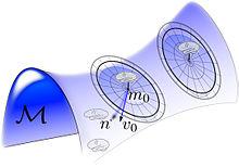 Orbits of brains associated to diffeomorphic group action on templates depicted via smooth flow associated to geodesic flows with random spray associatd to random generation of initial tangent space vector field ; published in.[9]
The random orbit model of Computational Anatomy first appeared in[128][129][130] modelling the change in coordinates associated to the randomness of the group acting on the templates, which induces the randomness on the source of images in the anatomical orbit of shapes and forms and resulting observations through the medical imaging devices. Such a random orbit model in which randomness on the group induces randomness on the images was examined for the Special Euclidean Group for object recognition in.[131]
Orbits of brains associated to diffeomorphic group action on templates depicted via smooth flow associated to geodesic flows with random spray associatd to random generation of initial tangent space vector field ; published in.[9]
The random orbit model of Computational Anatomy first appeared in[128][129][130] modelling the change in coordinates associated to the randomness of the group acting on the templates, which induces the randomness on the source of images in the anatomical orbit of shapes and forms and resulting observations through the medical imaging devices. Such a random orbit model in which randomness on the group induces randomness on the images was examined for the Special Euclidean Group for object recognition in.[131]
Depicted in the figure is a depiction of the random orbits around each exemplar, , generated by randomizing the flow by generating the initial tangent space vector field at the identity , and then generating random object .
The random orbit model induces the prior on shapes and images conditioned on a particular atlas . For this the generative model generates the mean field as a random change in coordinates of the template according to , where the diffeomorphic change in coordinates is generated randomly via the geodesic flows. The prior on random transformations on is induced by the flow , with constructed as a Gaussian random field prior . The density on the random observables at the output of the sensor are given by
Shown in the Figure on the right the cartoon orbit, are a random spray of the subcortical manifolds generated by randomizing the vector fields supported over the submanifolds.

Orbits of brains associated to diffeomorphic group action on templates depicted via smooth flow associated to geodesic flows with random spray associatd to random generation of initial tangent space vector field ; published in.[9]


The Bayesian model of computational anatomy
The central statistical model of Computational Anatomy in the context of medical imaging has been the source-channel model of Shannon theory;[128][129][130] the source is the deformable template of images , the channel outputs are the imaging sensors with observables (see Figure).
See The Bayesian model of computational anatomy for discussions (i) MAP estimation with multiple atlases, (ii) MAP segmentation with multiple atlases, MAP estimation of templates from populations.


Statistical shape theory in computational anatomy
Shape in computational anatomy is a local theory, indexing shapes and structures to templates to which they are bijectively mapped. Statistical shape in Computational Anatomy is the empirical study of diffeomorphic correspondences between populations and common template coordinate systems. Interestingly, this is a strong departure from Procrustes Analyses and shape theories pioneered by David G. Kendall[132] in that the central group of Kendall's theories are the finite-dimensional Lie groups, whereas the theories of shape in Computational Anatomy[133][134][135] have focused on the diffeomorphism group, which to first order via the Jacobian can be thought of as a field–thus infinite dimensional–of low-dimensional Lie groups of scale and rotations.
The random orbit model provides the natural setting to understand empirical shape and shape statistics within Computational anatomy since the non-linearity of the induced probability law on anatomical shapes and forms is induced via the reduction to the vector fields at the tangent space at the identity of the diffeomorphism group. The successive flow of the Euler equation induces the random space of shapes and forms .
Performing empirical statistics on this tangent space at the identity is the natural way for inducing probability laws on the statistics of shape. Since both the vector fields and the Eulerian momentum are in a Hilbert space the natural model is one of a Gaussian random field, so that given test function , then the inner-products with the test functions are Gaussian distributed with mean and covariance.
This is depicted in the accompanying figure where sub-cortical brain structures are depicted in a two-dimensional coordinate system based on inner products of their initial vector fields that generate them from the template is shown in a 2-dimensional span of the Hilbert space.


Template estimation from populations
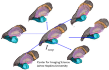 Depicting template estimation from multiplie subcortical surfaces in populations of MR images using the EM-algorithm solution of Ma.[136]
The study of shape and statistics in populations are local theories, indexing shapes and structures to templates to which they are bijectively mapped. Statistical shape is then the study of diffeomorphic correspondences relative to the template. A core operation is the generation of templates from populations, estimating a shape that is matched to the population. There are several important methods for generating templates including methods based on Frechet averaging,[137] and statistical approaches based on the expectation-maximization algorithm and the Bayes Random orbit models of Computational anatomy.[136][138] Shown in the accompanying figure is a subcortical template reconstruction from the population of MRI subjects.[139]
Depicting template estimation from multiplie subcortical surfaces in populations of MR images using the EM-algorithm solution of Ma.[136]
The study of shape and statistics in populations are local theories, indexing shapes and structures to templates to which they are bijectively mapped. Statistical shape is then the study of diffeomorphic correspondences relative to the template. A core operation is the generation of templates from populations, estimating a shape that is matched to the population. There are several important methods for generating templates including methods based on Frechet averaging,[137] and statistical approaches based on the expectation-maximization algorithm and the Bayes Random orbit models of Computational anatomy.[136][138] Shown in the accompanying figure is a subcortical template reconstruction from the population of MRI subjects.[139]

Depicting template estimation from multiplie subcortical surfaces in populations of MR images using the EM-algorithm solution of Ma.[136]
There are multiple methods for building a computing device based on DNA, each with its own advantages and disadvantages. Most of these build the basic logic gates (AND, OR, NOT) associated with digital logic from a DNA basis. Some of the different bases include DNAzymes, deoxyoligonucleotides, enzymes, toehold exchange.
DNAzymes
Catalytic DNA (deoxyribozyme or DNAzyme) catalyze a reaction when interacting with the appropriate input, such as a matching oligonucleotide. These DNAzymes are used to build logic gates analogous to digital logic in silicon; however, DNAzymes are limited to 1-, 2-, and 3-input gates with no current implementation for evaluating statements in series.
The DNAzyme logic gate changes its structure when it binds to a matching oligonucleotide and the fluorogenic substrate it is bonded to is cleaved free. While other materials can be used, most models use a fluorescence-based substrate because it is very easy to detect, even at the single molecule limit.[23] The amount of fluorescence can then be measured to tell whether or not a reaction took place. The DNAzyme that changes is then “used,” and cannot initiate any more reactions. Because of this, these reactions take place in a device such as a continuous stirred-tank reactor, where old product is removed and new molecules added.
Two commonly used DNAzymes are named E6 and 8-17. These are popular because they allow cleaving of a substrate in any arbitrary location.[24] Stojanovic and MacDonald have used the E6 DNAzymes to build the MAYA I[25] and MAYA II[26] machines, respectively; Stojanovic has also demonstrated logic gates using the 8-17 DNAzyme.[27] While these DNAzymes have been demonstrated to be useful for constructing logic gates, they are limited by the need for a metal cofactor to function, such as Zn2+ or Mn2+, and thus are not useful in vivo.[23][28]
A design called a stem loop, consisting of a single strand of DNA which has a loop at an end, are a dynamic structure that opens and closes when a piece of DNA bonds to the loop part. This effect has been exploited to create several logic gates. These logic gates have been used to create the computers MAYA I and MAYA II which can play tic-tac-toe to some extent.[29]
Enzyme
Enzyme based DNA computers are usually of the form of a simple Turing machine; there is analogous hardware, in the form of an enzyme, and software, in the form of DNA.[30]
Benenson, Shapiro and colleagues have demonstrated a DNA computer using the FokI enzyme[31] and expanded on their work by going on to show automata that diagnose and react to prostate cancer: under expression of the genes PPAP2B and GSTP1 and an over expression of PIM1 and HPN.[9] Their automata evaluated the expression of each gene, one gene at a time, and on positive diagnosis then released a single strand DNA molecule (ssDNA) that is an antisense for MDM2. MDM2 is a repressor of protein 53, which itself is a tumor suppressor.[32] On negative diagnosis it was decided to release a suppressor of the positive diagnosis drug instead of doing nothing. A limitation of this implementation is that two separate automata are required, one to administer each drug. The entire process of evaluation until drug release took around an hour to complete. This method also requires transition molecules as well as the FokI enzyme to be present. The requirement for the FokI enzyme limits application in vivo, at least for use in "cells of higher organisms".[33] It should also be pointed out that the 'software' molecules can be reused in this case.
Toehold exchange
DNA computers have also been constructed using the concept of toehold exchange. In this system, an input DNA strand binds to a sticky end, or toehold, on another DNA molecule, which allows it to displace another strand segment from the molecule. This allows the creation of modular logic components such as AND, OR, and NOT gates and signal amplifiers, which can be linked into arbitrarily large computers. This class of DNA computers does not require enzymes or any chemical capability of the DNA.[34]
Algorithmic self-assembly
 DNA arrays that display a representation of the Sierpinski gasket on their surfaces. Click the image for further details. Image from Rothemund et al., 2004.[35]
DNA nanotechnology has been applied to the related field of DNA computing. DNA tiles can be designed to contain multiple sticky ends with sequences chosen so that they act as Wang tiles. A DX array has been demonstrated whose assembly encodes an XOR operation; this allows the DNA array to implement a cellular automaton which generates a fractal called the Sierpinski gasket. This shows that computation can be incorporated into the assembly of DNA arrays, increasing its scope beyond simple periodic arrays.[35]
DNA arrays that display a representation of the Sierpinski gasket on their surfaces. Click the image for further details. Image from Rothemund et al., 2004.[35]
DNA nanotechnology has been applied to the related field of DNA computing. DNA tiles can be designed to contain multiple sticky ends with sequences chosen so that they act as Wang tiles. A DX array has been demonstrated whose assembly encodes an XOR operation; this allows the DNA array to implement a cellular automaton which generates a fractal called the Sierpinski gasket. This shows that computation can be incorporated into the assembly of DNA arrays, increasing its scope beyond simple periodic arrays.[35]

DNA arrays that display a representation of the Sierpinski gasket on their surfaces. Click the image for further details. Image from Rothemund et al., 2004.[35]
Tidak ada komentar:
Posting Komentar