

X . I
Light Forms Crystal-Like Structure On Computer Chip
Light Forms Crystal-Like Structure On Computer Chip at study science

Visible light shining
The study used microwaves.
.
"We build essentially an artificial atom, using lots of atoms acting in concert," Houck tells Popular Science, "What emerges is a quantum mechanical object that [at about half a millimeter] is visible on the classical scale."
For their study, that great big artificial atom sat on a computer chip, and researchers shined microwave photons on the system. The light particles were then trapped in the atom, forcing the photons to stay in one place. This, in turn, forced the photons to interact with one another, forming an organized crystal-like structure (or lattice).
Once the lattice formed, however, the researchers ran into two challenges: the system was hard to detect, and it was unstable. Light trapped in the lattice couldn't be observed directly without disrupting the entire system, so the researchers relied on indirect measurement of photons that escaped to "visualize" the event. But those escaping photons presented their own problem; as they left, the system degraded. In order to keep it going, more photons had to be constantly added in. This means the system was in a continuous state of change.
"We researchers are really good at studying static equilibriums," Houck says. He says there is value in studying dynamic, evolving physical phenomena. In the long term, he says this research, accomplished using components of a quantum computer, could pave the way for more advanced machines.
Technique that changes behaviour of photons could make quantum computers a reality
- Researchers created an 'artificial atom' and placed it close to photons
- Due to quantum mechanics, the photons inherit properties of the atom
- Normally photons do not interact with each other, but in this system the researchers found the photons interacted in some ways like particles
- The breakthrough could lead to the development of exotic materials that improve computing power beyond anything that exists today
Scientists are a step closer to creating quantum computers after making light behave like crystal.
The research team made the discovery by inventing a machine that uses quantum mechanics to make photons act like solid particles.
The breakthrough could lead to the development of exotic materials that improve computing power beyond anything that exists today.

Scientists are a step closer to creating quantum computers after making light behave like crystal. At first, photons in the experiment flow easily between two superconducting sites, producing the large waves shown at left. After a time, the scientists cause the light to 'freeze,' trapping the photons in place
'It's something that we have never seen before,' said Andrew Houck, an associate professor of Princeton University and one of the researchers. 'This is a new behaviour for light.'
As well as raising the possibility to create new materials, the researchers also intend to use the method to answer questions about the fundamental study of matter.
'We are interested in exploring - and ultimately controlling and directing – the flow of energy at the atomic level,' said Hakan Türeci, an assistant professor of electrical engineering and a member of the research team.'
The team's findings are part of an effort find out more about atomic behaviour by creating a device that can simulate the behaviour of subatomic particles.

'It's something that we have never seen before,' said Andrew Houck, an associate professor of Princeton University and one of the researchers. 'This is a new behaviour for light'
Such a tool could be an invaluable method for answering questions about atoms and molecules that are not answerable even with today's most advanced computers.
In part, that is because current computers operate under the rules of classical mechanics, which is a system that describes the everyday world containing things like bowling balls and planets.
But the world of atoms and photons obeys the rules of quantum mechanics, which include a number of strange and very counterintuitive features.
One of these odd properties is called 'entanglement' in which multiple particles become linked and can affect each other over long distances.
The difference between the quantum and classical rules limits a standard computer's ability to efficiently study quantum systems.
Because the computer operates under classical rules, it simply cannot grapple with many of the features of the quantum world.
To build their machine, the researchers created a structure made of superconducting materials that contains 100 billion atoms engineered to act as a single 'artificial atom.'
They placed the artificial atom close to a superconducting wire containing photons.

The team's findings are part of an effort to answer questions about atomic behaviour by creating a device that can simulate the behaviour of subatomic particles. Such a tool could be an invaluable method for answering questions about atoms and molecules that are not answerable even with today's most advanced computers
By the rules of quantum mechanics, the photons on the wire inherit some of the properties of the artificial atom – in a sense linking them.
Normally photons do not interact with each other, but in this system the researchers are able to create new behaviour in which the photons begin to interact in some ways like particles.
'We have used this blending together of the photons and the atom to artificially devise strong interactions among the photons,' said Darius Sadri, a postdoctoral researcher and one of the authors.
'These interactions then lead to completely new collective behaviour for light – akin to the phases of matter, like liquids and crystals, studied in condensed matter physics.'
That new behaviour could lead to a computer based on the rules of quantum mechanics that would have massive processing power.
It’s easy to shine light through a crystal, but researchers at Princeton University are turning light into crystals—essentially creating “solid light.”
“It’s something that we have never seen before,” Dr. Andrew Houck, associate professor of electrical engineering and one of the researchers, said in a written statement issued by the university. “This is a new behavior for light.”
New behavior is right. For generations, physics students have been taught that photons—the subatomic particles that make up light—don’t interact with each other. But the researchers were able to make photons interact very strongly.
To make that happen, the researchers assembled a structure of 100 billion atoms of superconducting material to create a sort of “artificial atom.” Then they placed the structure near a superconducting wire containing photons, which—as a result of the strange rules of quantum entanglement—caused the photons to take on some of the characteristics of the artificial atom.
“We have used this blending together of the photons and the atom to artificially devise strong interactions among the photons,” Darius Sadri, a postdoctoral researcher at the university and another one of the researchers, said in the statement. “These interactions then lead to completely new collective behavior for light—akin to the phases of matter, like liquids and crystals, studied in condensed matter physics.”
Pretty complicated stuff for sure. But what exactly is the point of the ongoing research?
One point is to work toward development of exotic materials, including room-temperature superconductors. Those are hypothetical materials that scientists believe could be used to create ultrasensitive sensors and computers of unprecedented speed—and which might even help solve the world’s energy problems.
How does light affect the
How do crystals get their color? The presence of different chemicals causes the variety of colors to different gemstones. Many gems are simply quartz crystals colored by the environments to which they are exposed. Amethyst gets its color from iron found at specific points in the crystalline structure. Topaz is an aluminium silicate - it comes in many colors due to the presence of different chemicals. The color of any compound (whether or not it is a crystal) depends on how the atoms and or molecules absorb light. Normally white light (what comes out of light bulbs) is considered to have all wavelengths (colors) of light in it. If you pass a white light through a colored compound some of the light is absorbed (we don't see the color which is absorbed, but we see the rest of the light) as it is reflected off the surface. This gives rise to the idea of "Complementary Colors". If a compound absorbs light of a certain color the compound appears to be the complimentary color. Here is a table of colors and their compliments: | |||||||||||||||||||||
| |||||||||||||||||||||


X . II
Explore the Lights


Fluorescent Minerals
Learn about the minerals and rocks that "glow" under ultraviolet light

Fluorescent minerals: One of the most spectacular museum exhibits is a dark room filled with fluorescent rocks and minerals that are illuminated with ultraviolet light. They glow with an amazing array of vibrant colors - in sharp contrast to the color of the rocks under conditions of normal illumination. The ultraviolet light activates these minerals and causes them to temporarily emit visible light of various colors. This light emission is known as "fluorescence." The wonderful photograph above shows a collection of fluorescent minerals.
What is a Fluorescent Mineral?
The color change of fluorescent minerals is most spectacular when they are illuminated in darkness by ultraviolet light (which is not visible to humans) and they release visible light. The photograph above is an example of this phenomenon.

How fluorescence works: Diagram that shows how photons and electrons interact to produce the fluorescence phenomenon.
Fluorescence in More Detail
Fluorescence in minerals occurs when a specimen is illuminated with specific wavelengths of light. Ultraviolet (UV) light, x-rays, and cathode rays are the typical types of light that trigger fluorescence. These types of light have the ability to excite susceptible electrons within the atomic structure of the mineral. These excited electrons temporarily jump up to a higher orbital within the mineral's atomic structure. When those electrons fall back down to their original orbital, a small amount of energy is released in the form of light. This release of light is known as fluorescence. [1]The wavelength of light released from a fluorescent mineral is often distinctly different from the wavelength of the incident light. This produces a visible change in the color of the mineral. This "glow" continues as long as the mineral is illuminated with light of the proper wavelength.
How Many Minerals Fluoresce in UV Light?
Most minerals do not have a noticeable fluorescence. Only about 15% of minerals have a fluorescence that is visible to people, and some specimens of those minerals will not fluoresce. Fluorescence usually occurs when specific impurities known as "activators" are present within the mineral. These activators are typically cations of metals such as: tungsten, molybdenum, lead, boron, titanium, manganese, uranium, and chromium. Rare earth elements such as europium, terbium, dysprosium, and yttrium are also known to contribute to the fluorescence phenomenon. Fluorescence can also be caused by crystal structural defects or organic impurities.In addition to "activator" impurities, some impurities have a dampening effect on fluorescence. If iron or copper are present as impurities, they can reduce or eliminate fluorescence. Furthermore, if the activator mineral is present in large amounts, that can reduce the fluorescence effect.
Most minerals fluoresce a single color. Other minerals have multiple colors of fluorescence. Calcite has been known to fluoresce red, blue, white, pink, green, and orange. Some minerals are known to exhibit multiple colors of fluorescence in a single specimen. These can be banded minerals that exhibit several stages of growth from parent solutions with changing compositions. Many minerals fluoresce one color under shortwave UV light and another color under longwave UV light.

Fluorite: Tumble-polished specimens of fluorite in normal light (top) and under shortwave ultraviolet light (bottom). The fluorescence appears to be related to the color and banding structure of the minerals in plain light, which could be related to their chemical composition.
Fluorite: The Original "Fluorescent Mineral"
One of the first people to observe fluorescence in minerals was George Gabriel Stokes in 1852. He noted the ability of fluorite to produce a blue glow when illuminated with invisible light "beyond the violet end of the spectrum." He called this phenomenon "fluorescence" after the mineral fluorite. The name has gained wide acceptance in mineralogy, gemology, biology, optics, commercial lighting and many other fields.Many specimens of fluorite have a strong enough fluorescence that the observer can take them outside, hold them in sunlight, then move them into shade and see a color change. Only a few minerals have this level of fluorescence. Fluorite typically glows a blue-violet color under shortwave and longwave light. Some specimens are known to glow a cream or white color. Many specimens do not fluoresce. Fluorescence in fluorite is thought to be caused by the presence of yttrium, europium, samarium or organic material as activators.

Fluorescent Dugway Geode: Many Dugway geodes contain fluorescent minerals and produce a spectacular display under UV light!
Fluorescent Geodes?
You might be surprised to learn that some people have found geodes with fluorescent minerals inside. Some of the Dugway geodes, found near the community of Dugway, Utah, are lined with chalcedony that produces a lime-green fluorescence caused by trace amounts of uranium.Dugway geodes are amazing for another reason. They formed several million years ago in the gas pockets of a rhyolite bed. Then, about 20,000 years ago they were eroded by wave action along the shoreline of a glacial lake and transported several miles to where they finally came to rest in lake sediments. Today, people dig them up and add them to geode and fluorescent mineral collections.

UV lamps: Three hobbyist-grade ultraviolet lamps used for fluorescent mineral viewing. At top left is a small "flashlight" style lamp that produces longwave UV light and is small enough to easily fit in a pocket. At top right is a small portable shortwave lamp. The lamp at bottom produces both longwave and shortwave light. The two windows are thick glass filters that eliminate visible light. The larger lamp is strong enough to use in taking photographs. UV-blocking glasses or goggles should always be worn when working with a UV lamp.
Lamps for Viewing Fluorescent Minerals
The lamps used to locate and study fluorescent minerals are very different from the ultraviolet lamps (called "black lights") sold in novelty stores. The novelty store lamps are not suitable for mineral studies for two reasons: 1) they emit longwave ultraviolet light (most fluorescent minerals respond to shortwave ultraviolet); and, 2) they emit a significant amount of visible light which interferes with accurate observation, but is not a problem for novelty use.Ultraviolet Wavelength Range | |||
| Wavelength | Abbreviations | ||
| Shortwave | 100-280nm | SW | UVC |
| Midwave | 280-315nm | MW | UVB |
| Longwave | 315-400nm | LW | UVA |
|

We offer a 4 watt UV lamp with a small filter window that is suitable for close examination of fluorescent minerals. We also offer a small collection of shortwave and longwave fluorescent mineral specimens.

Fluorescent spodumene: This spodumene (gem-variety kunzite) provides at least three important lessons in mineral fluorescence. All three photos show the same scatter of specimens. The top is in normal light, the center is in shortwave ultraviolet, and the bottom is in longwave ultraviolet. Lessons: 1) a single mineral can fluoresce with different colors; 2) the fluorescence can be different colors under shortwave and longwave light; and, 3) some specimens of a mineral will not fluoresce.
UV Lamp Safety
Ultraviolet wavelengths of light are present in sunlight. They are the wavelengths that can cause sunburn. UV lamps produce the same wavelengths of light along with shortwave UV wavelengths that are blocked by the ozone layer of Earth's atmosphere.Small UV lamps with just a few watts of power are safe for short periods of use. The user should not look into the lamp, shine the lamp directly onto the skin, or shine the lamp towards the face of a person or pet. Looking into the lamp can cause serious eye injury. Shining a UV lamp onto your skin can cause "sunburn."
Eye protection should be worn when using any UV lamp. Inexpensive UV blocking glasses, UV blocking safety glasses, or UV blocking prescription glasses provide adequate protection when using a low-voltage ultraviolet lamp for short periods of time for specimen examination.
The safety procedures of UV lamps used for fluorescent mineral studies should not be confused with those provided with the "blacklights" sold at party and novelty stores. "Blacklights" emit low-intensity longwave UV radiation. The shortwave UV radiation produced by a mineral study lamp contains the wavelengths associated with sunburn and eye injury. This is why mineral study lamps should be used with eye protection and handled more carefully than "blacklights."
UV lamps used to illuminate large mineral displays or used for outdoor field work have much higher voltages than the small UV lamps used for specimen examination by students. Eye protection and clothing that covers the arms, legs, feet and hands should be worn when using a high-voltage lamp.

UV Lamp and Minerals: The Geology.com Store offers an inexpensive ultraviolet lamp and a small fluorescent mineral collection. These are suitable for student use, and the lamp is accompanied by a pair of UV-blocking safety glasses.
Practical Uses of Mineral and Rock Fluorescence
Fluorescence has practical uses in mining, gemology, petrology, and mineralogy. The mineral scheelite, an ore of tungsten, typically has a bright blue fluorescence. Geologists prospecting for scheelite and other fluorescent minerals sometimes search for them at night with ultraviolet lamps.Geologists in the oil and gas industry sometimes examine drill cuttings and cores with UV lamps. Small amounts of oil in the pore spaces of the rock and mineral grains stained by oil will fluoresce under UV illumination. The color of the fluorescence can indicate the thermal maturity of the oil, with darker colors indicating heavier oils and lighter colors indicating lighter oils.
Fluorescent lamps can be used in underground mines to identify and trace ore-bearing rocks. They have also been used on picking lines to quickly spot valuable pieces of ore and separate them from waste.
Many gemstones are sometimes fluorescent, including ruby, kunzite, diamond, and opal. This property can sometimes be used to spot small stones in sediment or crushed ore. It can also be a way to associate stones with a mining locality. For example: light yellow diamonds with strong blue fluorescence are produced by South Africa's Premier Mine, and colorless stones with a strong blue fluorescence are produced by South Africa's Jagersfontein Mine. The stones from these mines are nicknamed "Premiers" and "Jagers."
In the early 1900s many diamond merchants would seek out stones with a strong blue fluorescence. They believed that these stones would appear more colorless (less yellow) when viewed in light with a high ultraviolet content. This eventually resulted in controlled lighting conditions for color grading diamonds.
Fluorescence is not routinely used in mineral identification. Most minerals are not fluorescent, and the property is unpredictable. Calcite provides a good example. Some calcite does not fluoresce. Specimens of calcite that do fluoresce glow in a variety of colors, including red, blue, white, pink, green, and orange. Fluorescence is rarely a diagnostic property.

Fluorescent ocean jasper: This image shows some pieces of tumbled ocean jasper under normal light (top), longwave ultraviolet (center), and shortwave ultraviolet (bottom). It shows how materials respond to different types of light.
Fluorescent Mineral Books
 |
| Fluorescent Mineral References |
| [1] Basic Concepts in Fluorescence: Michael W. Davidson and others, Optical Microscopy Primer, Florida State University, last accessed October 2016. [2] Fluorescent Minerals: James O. Hamblen, a website about fluorescent minerals, Georgia Tech, 2003. [3] The World of Fluorescent Minerals, Stuart Schneider, Schiffer Publishing Ltd., 2006. [4] Dugway Geodes page on the SpiritRock Shop website, last accessed May 2017. [5] Collecting Fluorescent Minerals, Stuart Schneider, Schiffer Publishing Ltd., 2004. [6] Ultraviolet Light Safety: Connecticut High School Science Safety, Connecticut State Department of Education, last accessed October 2016. [7] A Contribution to Understanding the Effect of Blue Fluorescence on the Appearance of Diamonds: Thomas M. Moses and others, Gems and Gemology, Gemological Institute of America, Winter 1997. |
Other Luminescence Properties
Fluorescence is one of several luminescence properties that a mineral might exhibit. Other luminescence properties include:PHOSPHORESCENCE In fluorescence, electrons excited by incoming photons jump up to a higher energy level and remain there for a tiny fraction of a second before falling back to the ground state and emitting fluorescent light. In phosphorescence, the electrons remain in the excited state orbital for a greater amount of time before falling. Minerals with fluorescence stop glowing when the light source is turned off. Minerals with phosphorescence can glow for a brief time after the light source is turned off. Minerals that are sometimes phosphorescent include calcite, celestite, colemanite, fluorite, sphalerite, and willemite.
THERMOLUMINESCENCE Thermoluminescence is the ability of a mineral to emit a small amount of light upon being heated. This heating might be to temperatures as low as 50 to 200 degrees Celsius - much lower than the temperature of incandescence. Apatite, calcite, chlorophane, fluorite, lepidolite, scapolite, and some feldspars are occasionally thermoluminescent.
TRIBOLUMINESCENCE Some minerals will emit light when mechanical energy is applied to them. These minerals glow when they are struck, crushed, scratched, or broken. This light is a result of bonds being broken within the mineral structure. The amount of light emitted is very small, and careful observation in the dark is often required. Minerals that sometimes display triboluminescence include amblygonite, calcite, fluorite, lepidolite, pectolite, quartz, sphalerite, and some feldspars.
X . III The Best Growing Conditions for Crystals
By Megan Shoop; Updated April 25, 2017
 Growing crystals serves as a way for students and children to learn about geology and how crystals and rock formations form over thousands of years. They can also experiment to see how different materials (sugar, salt and alum) make different kinds of crystals, as well as use different foundation pieces (yarn, pipe cleaners, bamboo skewers) to see how they affect how the crystals grow. However, without the right conditions, your crystals may not grow at all. While crystals don’t require much beyond patience, there are certain things you can do to make sure your experiments are successful.
Supersaturated Solution
No matter what material you choose, your water must be supersaturated with it for crystals to grow. This means you must dissolve as much of your chosen material into your water as possible. Materials dissolve faster in warm water, so it works better than cold, since the molecules move more in warm water. Simply pour one spoonful of your material at a time into the warm water and stir vigorously until it disappears. When your materials no longer disappear and settle on the bottom of your jar, the water is supersaturated and ready to go.Crystal Foundation
Porous materials work best as foundations for your crystals to grow easily. The air spaces allow the dissolved material to gain plenty of surface on the foundation material and attract more dissolved material as the water evaporates and leaves the solid crystals behind. Rough bamboo skewers, yarn, thread, ice cream sticks, pipe cleaners and even fabrics work very well as crystal foundations. Pencils, paper clips and other very smooth, dense materials will not work because there is nothing for the crystals to grab onto. Nylon thread and fishing line only work if you tie a seed crystal to the end; even then, the crystal will grow in one place instead of climbing the material.Light and Temperature
Because warmth is key to forming crystals, the jar’s surroundings should be warm also for optimum crystal growth. Warm air temperature aids water evaporation, causing the crystals to grow more quickly. Crystals will still grow in cooler temperatures, but it will take much longer for the water to evaporate. Crystal growth also requires light. Again, the crystals will eventually grow in the dark, but it will take a very long time. Light evaporates water as heat does; combine them by placing your jar on a warm, sunny windowsill and you should have crystals in a few days.X . III Electronic Energy Bands in Crystals
A study is made of the feasibility of calculating valence and excited electronic energy bands in crystals by making use of one-electron Bloch wave functions. The elements of the secular determinant for this method consist of Bloch sums of overlap and energy integrals. Although often used in evaluating these sums, the approximation of tight binding, which consists of neglecting integrals between non-neighboring atoms of the crystal, is very poor for metals, semiconductors, and valence crystals. By partially expanding each Bloch wave function in a three-dimensional Fourier series, these slowly convergent sums over ordinary space can be transformed into extremely rapidly convergent sums over momentum space. It can then be shown that, to an excellent approximation, the secular determinant vanishes identically. This peculiar behavior results from the poorness of the atomic correspondence for valence electrons. By a suitable transformation, a new secular determinant can be formed which does not vanish identically and which is suitable for numerical calculations. It is found that this secular determinant is identical with that obtained in the method of orthogonalized plane waves (plane waves made orthogonal to the inner-core Bloch wave functions).
Calculations are made on the lithium crystal in order to test how rapidly the energy converges to its limiting value as the order of the secular determinant is increased. For the valence band, this convergence is rapid. The effective mass of the electron at the bottom of the valence band is found to be closer to that of the free electron than are those of previous calculations on lithium. This is probably because of the use of a crystal potential here rather than an atomic potential. The former varies less rapidly than the latter over most of the unit cell of the crystal, and thus should result in a value of effective mass more nearly free-electron-like. Unlike previous calculations on lithium, the computed value of the width of the filled portion of the valence band agrees excellently with experiment. By making use of calculated transition probabilities between the valence band and the 1s level, a theoretical curve is drawn of the shape of the soft x-ray K emission band of lithium. The comparison with the shape of the experimental curve is only fair.
In solid-state physics, the electronic band structure (or simply band structure) of a solid describes the range of energies that an electron within the solid may have (called energy bands, allowed bands, or simply bands) and ranges of energy that it may not have (called band gaps or forbidden bands).
Band theory derives these bands and band gaps by examining the allowed quantum mechanical wave functions for an electron in a large, periodic lattice of atoms or molecules. Band theory has been successfully used to explain many physical properties of solids, such as electrical resistivity and optical absorption, and forms the foundation of the understanding of all solid-state devices (transistors, solar cells, etc.).
Why bands and band gaps occur

Showing how electronic band structure comes about by the hypothetical example of a large number of carbon atoms being brought together to form a diamond crystal. The graph (right) shows the energy levels as a function of the spacing between atoms. When the atoms are far apart (right side of graph) each atom has valence atomic orbitals p and s which have the same energy. However when the atoms come closer together their orbitals begin to overlap. Due to the Pauli Exclusion Principle each atomic orbital splits into N molecular orbitals each with a different energy, where N is the number of atoms in the crystal. Since N is such a large number, adjacent orbitals are extremely close together in energy so the orbitals can be considered a continuous energy band. a is the atomic spacing in an actual crystal of diamond. At that spacing the orbitals form two bands, called the valence and conduction bands, with a 5.5 eV band gap between them.
Similarly if a large number N of identical atoms come together to form a solid, such as a crystal lattice, the atoms' atomic orbitals overlap.[1] Since the Pauli exclusion principle dictates that no two electrons in the solid have the same quantum numbers, each atomic orbital splits into N discrete molecular orbitals, each with a different energy. Since the number of atoms in a macroscopic piece of solid is a very large number (N~1022) the number of orbitals is very large and thus they are very closely spaced in energy (of the order of 10−22 eV). The energy of adjacent levels is so close together that they can be considered as a continuum, an energy band.
This formation of bands is mostly a feature of the outermost electrons (valence electrons) in the atom, which are the ones responsible for chemical bonding and electrical conductivity. The inner electron orbitals do not overlap to a significant degree, so their bands are very narrow.
Band gaps are essentially leftover ranges of energy not covered by any band, a result of the finite widths of the energy bands. The bands have different widths, with the widths depending upon the degree of overlap in the atomic orbitals from which they arise. Two adjacent bands may simply not be wide enough to fully cover the range of energy. For example, the bands associated with core orbitals (such as 1s electrons) are extremely narrow due to the small overlap between adjacent atoms. As a result, there tend to be large band gaps between the core bands. Higher bands involve comparatively larger orbitals with more overlap, becoming progressively wider at higher energies so that there are no band gaps at higher energies.
Basic concepts
Assumptions and limits of band structure theory
Band theory is only an approximation to the quantum state of a solid, which applies to solids consisting of many identical atoms or molecules bonded together. These are the assumptions necessary for band theory to be valid:- Infinite-size system: For the bands to be continuous, the piece of material must consist of a large number of atoms. Since a macroscopic piece of material contains on the order of 1022 atoms, this is not a serious restriction; band theory even applies to microscopic-sized transistors in integrated circuits. With modifications, the concept of band structure can also be extended to systems which are only "large" along some dimensions, such as two-dimensional electron systems.
- Homogeneous system: Band structure is an intrinsic property of a material, which assumes that the material is homogeneous. Practically, this means that the chemical makeup of the material must be uniform throughout the piece.
- Non-interactivity: The band structure describes "single electron states". The existence of these states assumes that the electrons travel in a static potential without dynamically interacting with lattice vibrations, other electrons, photons, etc.
- Inhomogeneities and interfaces: Near surfaces, junctions, and other inhomogeneities, the bulk band structure is disrupted. Not only are there local small-scale disruptions (e.g., surface states or dopant states inside the band gap), but also local charge imbalances. These charge imbalances have electrostatic effects that extend deeply into semiconductors, insulators, and the vacuum (see doping, band bending).
- Along the same lines, most electronic effects (capacitance, electrical conductance, electric-field screening) involve the physics of electrons passing through surfaces and/or near interfaces. The full description of these effects, in a band structure picture, requires at least a rudimentary model of electron-electron interactions (see space charge, band bending).
- Small systems: For systems which are small along every dimension (e.g., a small molecule or a quantum dot), there is no continuous band structure. The crossover between small and large dimensions is the realm of mesoscopic physics.
- Strongly correlated materials (for example, Mott insulators) simply cannot be understood in terms of single-electron states. The electronic band structures of these materials are poorly defined (or at least, not uniquely defined) and may not provide useful information about their physical state.
Crystalline symmetry and wavevectors
.svg)

- ,

The wavevector takes on any value inside the Brillouin zone, which is a polyhedron in wavevector space that is related to the crystal's lattice. Wavevectors outside the Brillouin zone simply correspond to states that are physically identical to those states within the Brillouin zone. Special high symmetry points/lines in the Brillouin zone are assigned labels like Γ, Δ, Λ, Σ (see Fig 1).
It is difficult to visualize the shape of a band as a function of wavevector, as it would require a plot in four-dimensional space, E vs. kx, ky, kz. In scientific literature it is common to see band structure plots which show the values of En(k) for values of k along straight lines connecting symmetry points, often labelled Δ, Λ, Σ, or [100], [111], and [110], respectively. Another method for visualizing band structure is to plot a constant-energy isosurface in wavevector space, showing all of the states with energy equal to a particular value. The isosurface of states with energy equal to the Fermi level is known as the Fermi surface.
Energy band gaps can be classified using the wavevectors of the states surrounding the band gap:
- Direct band gap: the lowest-energy state above the band gap has the same k as the highest-energy state beneath the band gap.
- Indirect band gap: the closest states above and beneath the band gap do not have the same k value.
Asymmetry: Band structures in non-crystalline solids
Although electronic band structures are usually associated with crystalline materials, quasi-crystalline and amorphous solids may also exhibit band structures.These are somewhat more difficult to study theoretically since they lack the simple symmetry of a crystal, and it is not usually possible to determine a precise dispersion relation. As a result, virtually all of the existing theoretical work on the electronic band structure of solids has focused on crystalline materials.Density of states
The density of states function g(E) is defined as the number of electronic states per unit volume, per unit energy, for electron energies near E.The density of states function is important for calculations of effects based on band theory. In Fermi's Golden Rule, a calculation for the rate of optical absorption, it provides both the number of excitable electrons and the number of final states for an electron. It appears in calculations of electrical conductivity where it provides the number of mobile states, and in computing electron scattering rates where it provides the number of final states after scattering.[citation needed]
For energies inside a band gap, g(E) = 0.
Filling of bands

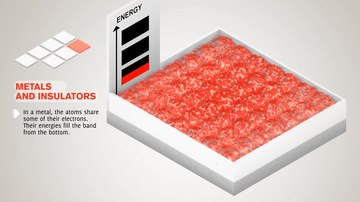
Filling of the electronic states in various types of materials at equilibrium. Here, height is energy while width is the density of available states for a certain energy in the material listed. The shade follows the Fermi–Dirac distribution (black = all states filled, white = no state filled). In metals and semimetals the Fermi level EF lies inside at least one band. In insulators and semiconductors the Fermi level is inside a band gap; however, in semiconductors the bands are near enough to the Fermi level to be thermally populated with electrons or holes.

- kBT is the product of Boltzmann's constant and temperature, and
- µ is the total chemical potential of electrons, or Fermi level (in semiconductor physics, this quantity is more often denoted EF). The Fermi level of a solid is directly related to the voltage on that solid, as measured with a voltmeter. Conventionally, in band structure plots the Fermi level is taken to be the zero of energy (an arbitrary choice).

Names of bands near the Fermi level (conduction band, valence band)
A solid has an infinite number of allowed bands, just as an atom has infinitely many energy levels. However, most of the bands simply have too high energy, and are usually disregarded under ordinary circumstances.[5] Conversely, there are very low energy bands associated with the core orbitals (such as 1s electrons). These low-energy core bands are also usually disregarded since they remain filled with electrons at all times, and are therefore inert.[6] Likewise, materials have several band gaps throughout their band structure.The most important bands and band gaps—those relevant for electronics and optoelectronics—are those with energies near the Fermi level. The bands and band gaps near the Fermi level are given special names, depending on the material:
- In a semiconductor or band insulator, the Fermi level is surrounded by a band gap, referred to as the band gap (to distinguish it from the other band gaps in the band structure). The closest band above the band gap is called the conduction band, and the closest band beneath the band gap is called the valence band. The name "valence band" was coined by analogy to chemistry, since in many semiconductors the valence band is built out of the valence orbitals.
- In a metal or semimetal, the Fermi level is inside of one or more allowed bands. In semimetals the bands are usually referred to as "conduction band" or "valence band" depending on whether the charge transport is more electron-like or hole-like, by analogy to semiconductors. In many metals, however, the bands are neither electron-like nor hole-like, and often just called "valence band" as they are made of valence orbitals.[7] The band gaps in a metal's band structure are not important for low energy physics, since they are too far from the Fermi level.
Theory of band structures in crystals
The ansatz is the special case of electron waves in a periodic crystal lattice using Bloch waves as treated generally in the dynamical theory of diffraction. Every crystal is a periodic structure which can be characterized by a Bravais lattice, and for each Bravais lattice we can determine the reciprocal lattice, which encapsulates the periodicity in a set of three reciprocal lattice vectors (b1,b2,b3). Now, any periodic potential V(r) which shares the same periodicity as the direct lattice can be expanded out as a Fourier series whose only non-vanishing components are those associated with the reciprocal lattice vectors. So the expansion can be written as:
From this theory, an attempt can be made to predict the band structure of a particular material, however most ab initio methods for electronic structure calculations fail to predict the observed band gap.
Nearly free electron approximation
In the nearly free electron approximation, interactions between electrons are completely ignored. This approximation allows use of Bloch's Theorem which states that electrons in a periodic potential have wavefunctions and energies which are periodic in wavevector up to a constant phase shift between neighboring reciprocal lattice vectors. The consequences of periodicity are described mathematically by the Bloch wavefunction:

- .

The NFE model works particularly well in materials like metals where distances between neighbouring atoms are small. In such materials the overlap of atomic orbitals and potentials on neighbouring atoms is relatively large. In that case the wave function of the electron can be approximated by a (modified) plane wave. The band structure of a metal like aluminium even gets close to the empty lattice approximation.
Tight binding model
The opposite extreme to the nearly free electron approximation assumes the electrons in the crystal behave much like an assembly of constituent atoms. This tight binding model assumes the solution to the time-independent single electron Schrödinger equation is well approximated by a linear combination of atomic orbitals .[9]

- ,


- ;


- .

KKR model
The simplest form of this approximation centers non-overlapping spheres (referred to as muffin tins) on the atomic positions. Within these regions, the potential experienced by an electron is approximated to be spherically symmetric about the given nucleus. In the remaining interstitial region, the screened potential is approximated as a constant. Continuity of the potential between the atom-centered spheres and interstitial region is enforced.A variational implementation was suggested by Korringa and by Kohn and Rostocker, and is often referred to as the KKR model.
Density-functional theory
In recent physics literature, a large majority of the electronic structures and band plots are calculated using density-functional theory (DFT), which is not a model but rather a theory, i.e., a microscopic first-principles theory of condensed matter physics that tries to cope with the electron-electron many-body problem via the introduction of an exchange-correlation term in the functional of the electronic density. DFT-calculated bands are in many cases found to be in agreement with experimentally measured bands, for example by angle-resolved photoemission spectroscopy (ARPES). In particular, the band shape is typically well reproduced by DFT. But there are also systematic errors in DFT bands when compared to experiment results. In particular, DFT seems to systematically underestimate by about 30-40% the band gap in insulators and semiconductors.It is commonly believed that DFT is a theory to predict ground state properties of a system only (e.g. the total energy, the atomic structure, etc.), and that excited state properties cannot be determined by DFT. This is a misconception. In principle, DFT can determine any property (ground state or excited state) of a system given a functional that maps the ground state density to that property. This is the essence of the Hohenberg–Kohn theorem.[15] In practice, however, no known functional exists that maps the ground state density to excitation energies of electrons within a material. Thus, what in the literature is quoted as a DFT band plot is a representation of the DFT Kohn–Sham energies, i.e., the energies of a fictive non-interacting system, the Kohn–Sham system, which has no physical interpretation at all. The Kohn–Sham electronic structure must not be confused with the real, quasiparticle electronic structure of a system, and there is no Koopman's theorem holding for Kohn–Sham energies, as there is for Hartree–Fock energies, which can be truly considered as an approximation for quasiparticle energies. Hence, in principle, Kohn–Sham based DFT is not a band theory, i.e., not a theory suitable for calculating bands and band-plots. In principle time-dependent DFT can be used to calculate the true band structure although in practice this is often difficult. A popular approach is the use of hybrid functionals, which incorporate a portion of Hartree–Fock exact exchange; this produces a substantial improvement in predicted bandgaps of semiconductors, but is less reliable for metals and wide-bandgap materials.
Green's function methods and the ab initio GW approximation
To calculate the bands including electron-electron interaction many-body effects, one can resort to so-called Green's function methods. Indeed, knowledge of the Green's function of a system provides both ground (the total energy) and also excited state observables of the system. The poles of the Green's function are the quasiparticle energies, the bands of a solid. The Green's function can be calculated by solving the Dyson equation once the self-energy of the system is known. For real systems like solids, the self-energy is a very complex quantity and usually approximations are needed to solve the problem. One such approximation is the GW approximation, so called from the mathematical form the self-energy takes as the product Σ = GW of the Green's function G and the dynamically screened interaction W. This approach is more pertinent when addressing the calculation of band plots (and also quantities beyond, such as the spectral function) and can also be formulated in a completely ab initio way. The GW approximation seems to provide band gaps of insulators and semiconductors in agreement with experiment, and hence to correct the systematic DFT underestimation.Mott insulators
Although the nearly free electron approximation is able to describe many properties of electron band structures, one consequence of this theory is that it predicts the same number of electrons in each unit cell. If the number of electrons is odd, we would then expect that there is an unpaired electron in each unit cell, and thus that the valence band is not fully occupied, making the material a conductor. However, materials such as CoO that have an odd number of electrons per unit cell are insulators, in direct conflict with this result. This kind of material is known as a Mott insulator, and requires inclusion of detailed electron-electron interactions (treated only as an averaged effect on the crystal potential in band theory) to explain the discrepancy. The Hubbard model is an approximate theory that can include these interactions. It can be treated non-perturbatively within the so-called dynamical mean field theory, which attempts to bridge the gap between the nearly free electron approximation and the atomic limit. Formally, however, the states are not non-interacting in this case and the concept of a band structure is not adequate to describe these cases.Others
Calculating band structures is an important topic in theoretical solid state physics. In addition to the models mentioned above, other models include the following:- Empty lattice approximation: the "band structure" of a region of free space that has been divided into a lattice.
- k·p perturbation theory is a technique that allows a band structure to be approximately described in terms of just a few parameters. The technique is commonly used for semiconductors, and the parameters in the model are often determined by experiment.
- The Kronig-Penney Model, a one-dimensional rectangular well model useful for illustration of band formation. While simple, it predicts many important phenomena, but is not quantitative.
- Hubbard model
Each model describes some types of solids very well, and others poorly. The nearly free electron model works well for metals, but poorly for non-metals. The tight binding model is extremely accurate for ionic insulators, such as metal halide salts (e.g. NaCl).
Band diagrams
To understand how band structure changes relative to the Fermi level in real space, a band structure plot is often first simplified in the form of a band diagram. In a band diagram the vertical axis is energy while the horizontal axis represents real space. Horizontal lines represent energy levels, while blocks represent energy bands. When the horizontal lines in these diagram are slanted then the energy of the level or band changes with distance. Diagrammatically, this depicts the presence of an electric field within the crystal system. Band diagrams are useful in relating the general band structure properties of different materials to one another when placed in contact with each other.X . IIII Quantum tunneling at Electronic so on light
Quantum tunnelling or tunneling (see spelling differences) refers to the quantum mechanical phenomenon where a particle tunnels through a barrier that it classically could not surmount. This plays an essential role in several physical phenomena, such as the nuclear fusion that occurs in main sequence stars like the Sun. It has important applications to modern devices such as the tunnel diode,quantum computing, and the scanning tunnelling microscope. The effect was predicted in the early 20th century and its acceptance as a general physical phenomenon came mid-century.[3]
Tunnelling is often explained using the Heisenberg uncertainty principle and the wave–particle duality of matter. Pure quantum mechanical concepts are central to the phenomenon, so quantum tunnelling is one of the novel implications of quantum mechanics. Quantum tunneling is projected to create physical limits to how small transistors can get, due to electrons being able to tunnel past them if they are too small.
Quantum tunnelling was developed from the study of radioactivity, The idea of the half-life and the possibility of predicting decay was created from their work.
Introduction to the concept

Animation showing the tunnel effect and its application to an STM


The reason for this difference comes from the treatment of matter in quantum mechanics as having properties of waves and particles. One interpretation of this duality involves the Heisenberg uncertainty principle, which defines a limit on how precisely the position and the momentum of a particle can be known at the same time.[4] This implies that there are no solutions with a probability of exactly zero (or one), though a solution may approach infinity if, for example, the calculation for its position was taken as a probability of 1, the other, i.e. its speed, would have to be infinity. Hence, the probability of a given particle's existence on the opposite side of an intervening barrier is non-zero, and such particles will appear on the 'other' (a semantically difficult word in this instance) side with a relative frequency proportional to this probability.

An electron wavepacket directed at a potential barrier. Note the dim spot on the right that represents tunnelling electrons.

Quantum tunnelling in the phase space formulation of quantum mechanics. Wigner function for tunnelling through the potential barrier in atomic units (a.u.). The solid lines represent the level set of the Hamiltonian .


The tunnelling problem
The wave function of a particle summarises everything that can be known about a physical system.[12] Therefore, problems in quantum mechanics center on the analysis of the wave function for a system. Using mathematical formulations of quantum mechanics, such as the Schrödinger equation, the wave function can be solved. This is directly related to the probability density of the particle's position, which describes the probability that the particle is at any given place. In the limit of large barriers, the probability of tunnelling decreases for taller and wider barriers.For simple tunnelling-barrier models, such as the rectangular barrier, an analytic solution exists. Problems in real life often do not have one, so "semiclassical" or "quasiclassical" methods have been developed to give approximate solutions to these problems, like the WKB approximation. Probabilities may be derived with arbitrary precision, constrained by computational resources, via Feynman's path integral method; such precision is seldom required in engineering practice.
Related phenomena
There are several phenomena that have the same behaviour as quantum tunnelling, and thus can be accurately described by tunnelling. Examples include the tunnelling of a classical wave-particle association,[13] evanescent wave coupling (the application of Maxwell's wave-equation to light) and the application of the non-dispersive wave-equation from acoustics applied to "waves on strings". Evanescent wave coupling, until recently, was only called "tunnelling" in quantum mechanics; now it is used in other contexts.These effects are modelled similarly to the rectangular potential barrier. In these cases, there is one transmission medium through which the wave propagates that is the same or nearly the same throughout, and a second medium through which the wave travels differently. This can be described as a thin region of medium B between two regions of medium A. The analysis of a rectangular barrier by means of the Schrödinger equation can be adapted to these other effects provided that the wave equation has travelling wave solutions in medium A but real exponential solutions in medium B.
In optics, medium A is a vacuum while medium B is glass. In acoustics, medium A may be a liquid or gas and medium B a solid. For both cases, medium A is a region of space where the particle's total energy is greater than its potential energy and medium B is the potential barrier. These have an incoming wave and resultant waves in both directions. There can be more mediums and barriers, and the barriers need not be discrete; approximations are useful in this case.
Applications
Tunnelling occurs with barriers of thickness around 1-3 nm and smaller,[14] but is the cause of some important macroscopic physical phenomena. For instance, tunnelling is a source of current leakage in very-large-scale integration (VLSI) electronics and results in the substantial power drain and heating effects that plague high-speed and mobile technology; it is considered the lower limit on how small computer chips can be made.[15] Tunnelling is a fundamental technique used to program the floating gates of FLASH memory, which is one of the most significant inventions that have shaped consumer electronics in the last two decades.Nuclear fusion in stars
Quantum tunnelling is essential for nuclear fusion in stars. Temperature and pressure in the core of stars are insufficient for nuclei to overcome the Coulomb barrier in order to achieve a thermonuclear fusion. However, there is some probability to penetrate the barrier due to quantum tunnelling. Though the probability is very low, the extreme number of nuclei in a star generates a steady fusion reaction over millions or even billions of years - a precondition for the evolution of life in insolation habitable zones.[16]Radioactive decay
Radioactive decay is the process of emission of particles and energy from the unstable nucleus of an atom to form a stable product. This is done via the tunnelling of a particle out of the nucleus (an electron tunnelling into the nucleus is electron capture). This was the first application of quantum tunnelling and led to the first approximations. Radioactive decay is also a relevant issue for astrobiology as this consequence of quantum tunnelling is creating a constant source of energy over a large period of time for environments outside the circumstellar habitable zone where insolation would not be possible (subsurface oceans) or effective.[16]Astrochemistry in interstellar clouds
By including quantum tunnelling the astrochemical syntheses of various molecules in interstellar clouds can be explained such as the synthesis of molecular hydrogen, water (ice) and the prebiotic important Formaldehyde.Quantum biology
Quantum tunnelling is among the central non trivial quantum effects in quantum biology. Here it is important both as electron tunnelling and proton tunnelling. Electron tunnelling is a key factor in many biochemical redox reactions (photosynthesis, cellular respiration) as well as enzymatic catalysis while proton tunnelling is a key factor in spontaneous mutation of DNA.[16]Spontaneous mutation of DNA occurs when normal DNA replication takes place after a particularly significant proton has defied the odds in quantum tunnelling in what is called "proton tunnelling"[17] (quantum biology). A hydrogen bond joins normal base pairs of DNA. There exists a double well potential along a hydrogen bond separated by a potential energy barrier. It is believed that the double well potential is asymmetric with one well deeper than the other so the proton normally rests in the deeper well. For a mutation to occur, the proton must have tunnelled into the shallower of the two potential wells. The movement of the proton from its regular position is called a tautomeric transition. If DNA replication takes place in this state, the base pairing rule for DNA may be jeopardised causing a mutation.[18] Per-Olov Lowdin was the first to develop this theory of spontaneous mutation within the double helix (quantum bio). Other instances of quantum tunnelling-induced mutations in biology are believed to be a cause of ageing and cancer.[19]
Cold emission
Cold emission of electrons is relevant to semiconductors and superconductor physics. It is similar to thermionic emission, where electrons randomly jump from the surface of a metal to follow a voltage bias because they statistically end up with more energy than the barrier, through random collisions with other particles. When the electric field is very large, the barrier becomes thin enough for electrons to tunnel out of the atomic state, leading to a current that varies approximately exponentially with the electric field.[20] These materials are important for flash memory, vacuum tubes, as well as some electron microscopes.Tunnel junction
A simple barrier can be created by separating two conductors with a very thin insulator. These are tunnel junctions, the study of which requires quantum tunnelling.[21] Josephson junctions take advantage of quantum tunnelling and the superconductivity of some semiconductors to create the Josephson effect. This has applications in precision measurements of voltages and magnetic fields,[20] as well as the multijunction solar cell.
A working mechanism of a resonant tunnelling diode device, based on the phenomenon of quantum tunnelling through the potential barriers.
Tunnel diode
Diodes are electrical semiconductor devices that allow electric current flow in one direction more than the other. The device depends on a depletion layer between N-type and P-type semiconductors to serve its purpose; when these are very heavily doped the depletion layer can be thin enough for tunnelling. Then, when a small forward bias is applied the current due to tunnelling is significant. This has a maximum at the point where the voltage bias is such that the energy level of the p and n conduction bands are the same. As the voltage bias is increased, the two conduction bands no longer line up and the diode acts typically.[22]Because the tunnelling current drops off rapidly, tunnel diodes can be created that have a range of voltages for which current decreases as voltage is increased. This peculiar property is used in some applications, like high speed devices where the characteristic tunnelling probability changes as rapidly as the bias voltage.[22]
The resonant tunnelling diode makes use of quantum tunnelling in a very different manner to achieve a similar result. This diode has a resonant voltage for which there is a lot of current that favors a particular voltage, achieved by placing two very thin layers with a high energy conductance band very near each other. This creates a quantum potential well that have a discrete lowest energy level. When this energy level is higher than that of the electrons, no tunnelling will occur, and the diode is in reverse bias. Once the two voltage energies align, the electrons flow like an open wire. As the voltage is increased further tunnelling becomes improbable and the diode acts like a normal diode again before a second energy level becomes noticeable.[23]
Tunnel field-effect transistors
A European research project has demonstrated field effect transistors in which the gate (channel) is controlled via quantum tunnelling rather than by thermal injection, reducing gate voltage from ~1 volt to 0.2 volts and reducing power consumption by up to 100×. If these transistors can be scaled up into VLSI chips, they will significantly improve the performance per power of integrated circuits.[24]Quantum conductivity
While the Drude model of electrical conductivity makes excellent predictions about the nature of electrons conducting in metals, it can be furthered by using quantum tunnelling to explain the nature of the electron's collisions.[20] When a free electron wave packet encounters a long array of uniformly spaced barriers the reflected part of the wave packet interferes uniformly with the transmitted one between all barriers so that there are cases of 100% transmission. The theory predicts that if positively charged nuclei form a perfectly rectangular array, electrons will tunnel through the metal as free electrons, leading to an extremely high conductance, and that impurities in the metal will disrupt it significantly.[20]Scanning tunnelling microscope
The scanning tunnelling microscope (STM), invented by Gerd Binnig and Heinrich Rohrer, may allow imaging of individual atoms on the surface of a material.[20] It operates by taking advantage of the relationship between quantum tunnelling with distance. When the tip of the STM's needle is brought very close to a conduction surface that has a voltage bias, by measuring the current of electrons that are tunnelling between the needle and the surface, the distance between the needle and the surface can be measured. By using piezoelectric rods that change in size when voltage is applied over them the height of the tip can be adjusted to keep the tunnelling current constant. The time-varying voltages that are applied to these rods can be recorded and used to image the surface of the conductor.[20] STMs are accurate to 0.001 nm, or about 1% of atomic diameter.Faster than light
It is possible for spin zero particles to travel faster than the speed of light when tunnelling.[3] This apparently violates the principle of causality, since there will be a frame of reference in which it arrives before it has left. However, careful analysis of the transmission of the wave packet shows that there is actually no violation of relativity theory. In 1998, Francis E. Low reviewed briefly the phenomenon of zero time tunnelling.[25] More recently experimental tunnelling time data of phonons, photons, and electrons have been published by Günter Nimtz.[26]Mathematical discussions of quantum tunnelling
The following subsections discuss the mathematical formulations of quantum tunnelling.The Schrödinger equation
The time-independent Schrödinger equation for one particle in one dimension can be written as- or


The solutions of the Schrödinger equation take different forms for different values of x, depending on whether M(x) is positive or negative. When M(x) is constant and negative, then the Schrödinger equation can be written in the form


The mathematics of dealing with the situation where M(x) varies with x is difficult, except in special cases that usually do not correspond to physical reality. A discussion of the semi-classical approximate method, as found in physics textbooks, is given in the next section. A full and complicated mathematical treatment appears in the 1965 monograph by Fröman and Fröman noted below. Their ideas have not been incorporated into physics textbooks, but their corrections have little quantitative effect.
The WKB approximation
The wave function is expressed as the exponential of a function:- , where


- , where A(x) and B(x) are real-valued functions.

- .


- ,


- .

Case 1 If the amplitude varies slowly as compared to the phase and


- which corresponds to classical motion. Resolving the next order of expansion yields
![\Psi(x) \approx C \frac{ e^{i \int dx \sqrt{\frac{2m}{\hbar^2} \left( E - V(x) \right)} + \theta} }{\sqrt[4]{\frac{2m}{\hbar^2} \left( E - V(x) \right)}}](https://wikimedia.org/api/rest_v1/media/math/render/svg/a5ee1989ca3279bca4fb4f1fea48a0c48c724f1e)
- If the phase varies slowly as compared to the amplitude, and


- which corresponds to tunnelling. Resolving the next order of the expansion yields
![\Psi(x) \approx \frac{ C_{+} e^{+\int dx \sqrt{\frac{2m}{\hbar^2} \left( V(x) - E \right)}} + C_{-} e^{-\int dx \sqrt{\frac{2m}{\hbar^2} \left( V(x) - E \right)}}}{\sqrt[4]{\frac{2m}{\hbar^2} \left( V(x) - E \right)}}](https://wikimedia.org/api/rest_v1/media/math/render/svg/e4bff4af65fcfda75cb594e31f867ce95e972d22)

To start, choose a classical turning point, and expand in a power series about :


- .

- .

![\Psi(x) = C_A Ai\left( \sqrt[3]{v_1} (x - x_1) \right) + C_B Bi\left( \sqrt[3]{v_1} (x - x_1) \right)](https://wikimedia.org/api/rest_v1/media/math/render/svg/735a1e9ea0d738f9153e0ceab4ef3171c08a6215)
Hence, the Airy function solutions will asymptote into sine, cosine and exponential functions in the proper limits. The relationships between and are


- ,
![T(E)=e^{{-2\int _{{x_{1}}}^{{x_{2}}}{\mathrm {d}}x{\sqrt {{\frac {2m}{\hbar ^{2}}}\left[V(x)-E\right]}}}}](https://wikimedia.org/api/rest_v1/media/math/render/svg/772eea412ba70d586ceb13d18765e61b6d552cbd)

For a rectangular barrier, this expression is simplified to:
- .

X . IIIII Quantum teleportation
Quantum teleportation is a process by which quantum information (e.g. the exact state of an atom or photon) can be transmitted (exactly, in principle) from one location to another, with the help of classical communication and previously shared quantum entanglement between the sending and receiving location. Because it depends on classical communication, which can proceed no faster than the speed of light, it cannot be used for faster-than-light transport or communication of classical bits. While it has proven possible to teleport one or more qubits of information between two (entangled) atoms,[1][2][3] this has not yet been achieved between molecules or anything larger.
Although the name is inspired by the teleportation commonly used in fiction, there is no relationship outside the name, because quantum teleportation concerns only the transfer of information. Quantum teleportation is not a form of transport, but of communication; it provides a way of transporting a qubit from one location to another, without having to move a physical particle along with it.
The seminal paper[4] first expounding the idea of quantum teleportation was published by C. H. Bennett, G. Brassard, C. Crépeau, R. Jozsa, A. Peres and W. K. Wootters in 1993.[5] Since then, quantum teleportation was first realized with single photons [6] and later demonstrated with various material systems such as atoms, ions, electrons and superconducting circuits. The record distance for quantum teleportation is 143 km (89 mi).[7]
In October 2015, scientists from the Kavli Institute of Nanoscience of the Delft University of Technology reported that the quantum nonlocality phenomenon is supported at the 96% confidence level based on a "loophole-free Bell test" study.[8][9] These results were confirmed by two studies with statistical significance over 5 standard deviations which were published in December 2015 .
Non-technical summary
In matters relating to quantum or classical information theory, it is convenient to work with the simplest possible unit of information, the two-state system. In classical information this is a bit, commonly represented using one or zero (or true or false). The quantum analog of a bit is a quantum bit, or qubit. Qubits encode a type of information, called quantum information, which differs sharply from "classical" information. For example, quantum information can be neither copied (the no-cloning theorem) nor destroyed (the no-deleting theorem).Quantum teleportation provides a mechanism of moving a qubit from one location to another, without having to physically transport the underlying particle that a qubit is normally attached to. Much like the invention of the telegraph allowed classical bits to be transported at high speed across continents, quantum teleportation holds the promise that one day, qubits could be moved likewise. However, as of 2013[update], only photons and single atoms have been employed as information bearers.
The movement of qubits does require the movement of "things"; in particular, the actual teleportation protocol requires that an entangled quantum state or Bell state be created, and its two parts shared between two locations (the source and destination, or Alice and Bob). In essence, a certain kind of "quantum channel" between two sites must be established first, before a qubit can be moved. Teleportation also requires a classical information link to be established, as two classical bits must be transmitted to accompany each qubit. The reason for this is that the results of the measurements must be communicated, and this must be done over ordinary classical communication channels. The need for such links may, at first, seem disappointing; however, this is not unlike ordinary communications, which requires wires, radios or lasers. What's more, Bell states are most easily shared using photons from lasers, and so teleportation could be done, in principle, through open space.
The quantum states of single atoms have been teleported.[1][2][3] An atom consists of several parts: the qubits in the electronic state or electron shells surrounding the atomic nucleus, the qubits in the nucleus itself, and, finally, the electrons, protons and neutrons making up the atom. Physicists have teleported the qubits encoded in the electronic state of atoms; they have not teleported the nuclear state, nor the nucleus itself. It is therefore false to say "an atom has been teleported". It has not. The quantum state of an atom has. Thus, performing this kind of teleportation requires a stock of atoms at the receiving site, available for having qubits imprinted on them. The importance of teleporting nuclear state is unclear: nuclear state does affect the atom, e.g. in hyperfine splitting, but whether such state would need to be teleported in some futuristic "practical" application is debatable.
An important aspect of quantum information theory is entanglement, which imposes statistical correlations between otherwise distinct physical systems. These correlations hold even when measurements are chosen and performed independently, out of causal contact from one another, as verified in Bell test experiments. Thus, an observation resulting from a measurement choice made at one point in spacetime seems to instantaneously affect outcomes in another region, even though light hasn't yet had time to travel the distance; a conclusion seemingly at odds with Special relativity (EPR paradox). However such correlations can never be used to transmit any information faster than the speed of light, a statement encapsulated in the no-communication theorem. Thus, teleportation, as a whole, can never be superluminal, as a qubit cannot be reconstructed until the accompanying classical information arrives.
Understanding quantum teleportation requires a good grounding in finite-dimensional linear algebra, Hilbert spaces and projection matrixes. A qubit is described using a two-dimensional complex number-valued vector space (a Hilbert space), which are the primary basis for the formal manipulations given below. A working knowledge of quantum mechanics is not absolutely required to understand the mathematics of quantum teleportation, although without such acquaintance, the deeper meaning of the equations may remain quite mysterious.
Protocol
The prerequisites for quantum teleportation are a qubit that is to be teleported, a conventional communication channel capable of transmitting two classical bits (i.e., one of four states), and means of generating an entangled EPR pair of qubits, transporting each of these to two different locations, A and B, performing a Bell measurement on one of the EPR pair qubits, and manipulating the quantum state of the other of the pair. The protocol is then as follows:
- An EPR pair is generated, one qubit sent to location A, the other to B.
- At location A, a Bell measurement of the EPR pair qubit and the qubit to be teleported (the quantum state ) is performed, yielding one of four measurement outcomes, which can be encoded in two classical bits of information. Both qubits at location A are then discarded.
- Using the classical channel, the two bits are sent from A to B. (This is the only potentially time-consuming step after step 1, due to speed-of-light considerations.)
- As a result of the measurement performed at location A, the EPR pair qubit at location B is in one of four possible states. Of these four possible states, one is identical to the original quantum state , and the other three are closely related. Which of these four possibilities actually obtains is encoded in the two classical bits. Knowing this, the qubit at location B is modified in one of three ways, or not at all, to result in a qubit identical to , the qubit that was chosen for teleportation.

Experimental results and records
Work in 1998 verified the initial predictions,[12] and the distance of teleportation was increased in August 2004 to 600 meters, using optical fiber.[13] Subsequently, the record distance for quantum teleportation has been gradually increased to 16 km,[14] then to 97 km,[15] and is now 143 km (89 mi), set in open air experiments done between two of the Canary Islands.[7] There has been a recent record set (as of September 2015) using superconducting nanowire detectors that reached the distance of 102 km (63 mi) over optical fiber.[16] For material systems, the record distance is 21 m.[17]A variant of teleportation called "open-destination" teleportation, with receivers located at multiple locations, was demonstrated in 2004 using five-photon entanglement.[18] Teleportation of a composite state of two single photons has also been realized.[19] In April 2011, experimenters reported that they had demonstrated teleportation of wave packets of light up to a bandwidth of 10 MHz while preserving strongly nonclassical superposition states.[20][21] In August 2013, the achievement of "fully deterministic" quantum teleportation, using a hybrid technique, was reported.[22] On 29 May 2014, scientists announced a reliable way of transferring data by quantum teleportation. Quantum teleportation of data had been done before but with highly unreliable methods.[23][24] On 26 February 2015, scientists at the University of Science and Technology of China in Hefei, led by Chao-yang Lu and Jian-Wei Pan carried out the first experiment teleporting multiple degrees of freedom of a quantum particle. They managed to teleport the quantum information from ensemble of rubidium atoms to another ensemble of rubidium atoms over a distance of 150 metres using entangled photons[25][26]
Researchers have also successfully used quantum teleportation to transmit information between clouds of gas atoms, notable because the clouds of gas are macroscopic atomic ensembles.[27][28]
Formal presentation
There are a variety of ways in which the teleportation protocol can be written mathematically. Some are very compact but abstract, and some are verbose but straightforward and concrete. The presentation below is of the latter form: verbose, but has the benefit of showing each quantum state simply and directly. Later sections review more compact notations.The teleportation protocol begins with a quantum state or qubit , in Alice's possession, that she wants to convey to Bob. This qubit can be written generally, in bra–ket notation, as:


Next, the protocol requires that Alice and Bob share a maximally entangled state. This state is fixed in advance, by mutual agreement between Alice and Bob, and can be any one of the four Bell states shown. It does not matter which one.
- ,
- ,
- ,
- .


At this point, Alice has two particles (C, the one she wants to teleport, and A, one of the entangled pair), and Bob has one particle, B. In the total system, the state of these three particles is given by


- .


The result of Alice's Bell measurement tells her which of the above four states the system is in. She can now send her result to Bob through a classical channel. Two classical bits can communicate which of the four results she obtained.
After Bob receives the message from Alice, he will know which of the four states his particle is in. Using this information, he performs a unitary operation on his particle to transform it to the desired state :

- If Alice indicates her result is , Bob knows his qubit is already in the desired state and does nothing. This amounts to the trivial unitary operation, the identity operator.
- If the message indicates , Bob would send his qubit through the unitary quantum gate given by the Pauli matrix


- If Alice's message corresponds to , Bob applies the gate


- Finally, for the remaining case, the appropriate gate is given by

Some remarks:
- After this operation, Bob's qubit will take on the state , and Alice's qubit becomes an (undefined) part of an entangled state. Teleportation does not result in the copying of qubits, and hence is consistent with the no cloning theorem.
- There is no transfer of matter or energy involved. Alice's particle has not been physically moved to Bob; only its state has been transferred. The term "teleportation", coined by Bennett, Brassard, Crépeau, Jozsa, Peres and Wootters, reflects the indistinguishability of quantum mechanical particles.
- For every qubit teleported, Alice needs to send Bob two classical bits of information. These two classical bits do not carry complete information about the qubit being teleported. If an eavesdropper intercepts the two bits, she may know exactly what Bob needs to do in order to recover the desired state. However, this information is useless if she cannot interact with the entangled particle in Bob's possession.

Alternative notations


Quantum circuit representation of quantum teleportation


Entanglement swapping
Teleportation can be applied not just to pure states, but also mixed states, that can be regarded as the state of a single subsystem of an entangled pair. The so-called entanglement swapping is a simple and illustrative example.If Alice has a particle which is entangled with a particle owned by Bob, and Bob teleports it to Carol, then afterwards, Alice's particle is entangled with Carol's.
A more symmetric way to describe the situation is the following: Alice has one particle, Bob two, and Carol one. Alice's particle and Bob's first particle are entangled, and so are Bob's second and Carol's particle:
                      ___
                     /   \
 Alice-:-:-:-:-:-Bob1 -:- Bob2-:-:-:-:-:-Carol
                     \___/
Now, if Bob does a projective measurement on his two particles in the Bell state basis and communicates the results to Carol, as per the teleportation scheme described above, the state of Bob's first particle can be teleported to Carol's. Although Alice and Carol never interacted with each other, their particles are now entangled.A detailed diagrammatic derivation of entanglement swapping has been given by Bob Coecke,[31] presented in terms of categorical quantum mechanics.
N-state particles
One can imagine how the teleportation scheme given above might be extended to N-state particles, i.e. particles whose states lie in the N dimensional Hilbert space. The combined system of the three particles now has an dimensional state space. To teleport, Alice makes a partial measurement on the two particles in her possession in some entangled basis on the dimensional subsystem. This measurement has equally probable outcomes, which are then communicated to Bob classically. Bob recovers the desired state by sending his particle through an appropriate unitary gate.

Logic gate teleportation
In general, mixed states ρ may be transported, and a linear transformation ω applied during teleportation, thus allowing data processing of quantum information. This is one of the foundational building blocks of quantum information processing. This is demonstrated below.General description
A general teleportation scheme can be described as follows. Three quantum systems are involved. System 1 is the (unknown) state ρ to be teleported by Alice. Systems 2 and 3 are in a maximally entangled state ω that are distributed to Alice and Bob, respectively. The total system is then in the state


Taking adjoint maps in the Heisenberg picture, the success condition becomes


Further details
The proposed channel Φ can be described more explicitly. To begin teleportation, Alice performs a local measurement on the two subsystems (1 and 2) in her possession. Assume the local measurement have effects


Therefore, the channel Φ is defined by


Local explanation of the phenomenon
A local explanation of quantum teleportation is put forward by David Deutsch and Patrick Hayden, with respect to the many-worlds interpretation of Quantum mechanics. Their paper asserts that the two bits that Alice sends Bob contain "locally inaccessible information" resulting in the teleportation of the quantum state. "The ability of quantum information to flow through a classical channel ..., surviving decoherence, is ... the basis of quantum teleportation."X . IIIIII Quantum computing
Quantum computing studies theoretical computation systems (quantum computers) that make direct use of quantum-mechanical phenomena, such as superposition and entanglement, to perform operations on data.[1] Quantum computers are different from binary digital electronic computers based on transistors. Whereas common digital computing requires that the data be encoded into binary digits (bits), each of which is always in one of two definite states (0 or 1), quantum computation uses quantum bits, which can be in superpositions of states. A quantum Turing machine is a theoretical model of such a computer, and is also known as the universal quantum computer. The field of quantum computing was initiated by the work of Paul Benioff[2] and Yuri Manin in 1980,[3] Richard Feynman in 1982,[4] and David Deutsch in 1985.[5] A quantum computer with spins as quantum bits was also formulated for use as a quantum space–time in 1968.[6]
As of 2017[update], the development of actual quantum computers is still in its infancy, but experiments have been carried out in which quantum computational operations were executed on a very small number of quantum bits.[7] Both practical and theoretical research continues, and many national governments and military agencies are funding quantum computing research in an effort to develop quantum computers for civilian, business, trade, environmental and national security purposes, such as cryptanalysis.[8]
Large-scale quantum computers would theoretically be able to solve certain problems much more quickly than any classical computers that use even the best currently known algorithms, like integer factorization using Shor's algorithm or the simulation of quantum many-body systems. There exist quantum algorithms, such as Simon's algorithm, that run faster than any possible probabilistic classical algorithm.[9] A classical computer could in principle (with exponential resources) simulate a quantum algorithm, as quantum computation does not violate the Church–Turing thesis.[10]:202 On the other hand, quantum computers may be able to efficiently solve problems which are not practically feasible on classical computers.
 The Bloch sphere is a representation of a qubit, the fundamental building block of quantum computers
 Basis
A classical computer has a memory made up of bits, where each bit is represented by either a one or a zero. A quantum computer maintains a sequence of qubits. A single qubit can represent a one, a zero, or any quantum superposition of those two qubit states;[10]:13–16 a pair of qubits can be in any quantum superposition of 4 states,[10]:16 and three qubits in any superposition of 8 states. In general, a quantum computer with qubits can be in an arbitrary superposition of up to different states simultaneously[10]:17 (this compares to a normal computer that can only be in one of these states at any one time). A quantum computer operates by setting the qubits in a perfect drift[clarification needed] that represents the problem at hand and by manipulating those qubits with a fixed sequence of quantum logic gates. The sequence of gates to be applied is called a quantum algorithm. The calculation ends with a measurement, collapsing the system of qubits into one of the pure states, where each qubit is zero or one, decomposing into a classical state. The outcome can therefore be at most classical bits of information. Quantum algorithms are often probabilistic, in that they provide the correct solution only with a certain known probability.[11] Note that the term non-deterministic computing must not be used in that case to mean probabilistic (computing), because the term non-deterministic has a different meaning in computer science.

An example of an implementation of qubits of a quantum computer could start with the use of particles with two spin states: "down" and "up" (typically written and , or and ). This is true because any such system can be mapped onto an effective spin-1/2 system.


Principles of operation
A quantum computer with a given number of qubits is fundamentally different from a classical computer composed of the same number of classical bits. For example, representing the state of an n-qubit system on a classical computer requires the storage of 2n complex coefficients, while to characterize the state of a classical n-bit system it is sufficient to provide the values of the n bits, that is, only n numbers. Although this fact may seem to indicate that qubits can hold exponentially more information than their classical counterparts, care must be taken not to overlook the fact that the qubits are only in a probabilistic superposition of all of their states. This means that when the final state of the qubits is measured, they will only be found in one of the possible configurations they were in before the measurement. It is generally incorrect to think of a system of qubits as being in one particular state before the measurement, since the fact that they were in a superposition of states before the measurement was made directly affects the possible outcomes of the computation.
Qubits are made up of controlled particles and the means of control (e.g. devices that trap particles and switch them from one state to another).[12]

The state of a three-qubit quantum computer is similarly described by an eight-dimensional vector (or a one dimensional vector with each vector node holding the amplitude and the state as the bit string of qubits). Here, however, the coefficients are complex numbers, and it is the sum of the squares of the coefficients' absolute values, , that must equal 1. For each , the absolute value squared gives the probability of the system being found after a measurement in the -th state. However, because a complex number encodes not just a magnitude but also a direction in the complex plane, the phase difference between any two coefficients (states) represents a meaningful parameter. This is a fundamental difference between quantum computing and probabilistic classical computing.[13]


If you measure the three qubits, you will observe a three-bit string. The probability of measuring a given string is the squared magnitude of that string's coefficient (i.e., the probability of measuring 000 = , the probability of measuring 001 = , etc.). Thus, measuring a quantum state described by complex coefficients gives the classical probability distribution and we say that the quantum state "collapses" to a classical state as a result of making the measurement.


An eight-dimensional vector can be specified in many different ways depending on what basis is chosen for the space. The basis of bit strings (e.g., 000, 001, …, 111) is known as the computational basis. Other possible bases are unit-length, orthogonal vectors and the eigenvectors of the Pauli-x operator. Ket notation is often used to make the choice of basis explicit. For example, the state in the computational basis can be written as:
- where, e.g.,


Using the eigenvectors of the Pauli-x operator, a single qubit is and .


Operation
| Unsolved problem in physics: |

Finally, upon termination of the algorithm, the result needs to be read off. In the case of a classical computer, we sample from the probability distribution on the three-bit register to obtain one definite three-bit string, say 000. Quantum mechanically, we measure the three-qubit state, which is equivalent to collapsing the quantum state down to a classical distribution (with the coefficients in the classical state being the squared magnitudes of the coefficients for the quantum state, as described above), followed by sampling from that distribution. This destroys the original quantum state. Many algorithms will only give the correct answer with a certain probability. However, by repeatedly initializing, running and measuring the quantum computer's results, the probability of getting the correct answer can be increased. In contrast, counterfactual quantum computation allows the correct answer to be inferred when the quantum computer is not actually running in a technical sense, though earlier initialization and frequent measurements are part of the counterfactual computation protocol.
For more details on the sequences of operations used for various quantum algorithms, see universal quantum computer, Shor's algorithm, Grover's algorithm, Deutsch–Jozsa algorithm, amplitude amplification, quantum Fourier transform, quantum gate, quantum adiabatic algorithm and quantum error correction.
Potential
Integer factorization, which underpins the security of public key cryptographic systems, is believed to be computationally infeasible with an ordinary computer for large integers if they are the product of few prime numbers (e.g., products of two 300-digit primes).[14] By comparison, a quantum computer could efficiently solve this problem using Shor's algorithm to find its factors. This ability would allow a quantum computer to decrypt many of the cryptographic systems in use today, in the sense that there would be a polynomial time (in the number of digits of the integer) algorithm for solving the problem. In particular, most of the popular public key ciphers are based on the difficulty of factoring integers or the discrete logarithm problem, both of which can be solved by Shor's algorithm. In particular the RSA, Diffie-Hellman, and Elliptic curve Diffie-Hellman algorithms could be broken. These are used to protect secure Web pages, encrypted email, and many other types of data. Breaking these would have significant ramifications for electronic privacy and security.However, other cryptographic algorithms do not appear to be broken by those algorithms.[15][16] Some public-key algorithms are based on problems other than the integer factorization and discrete logarithm problems to which Shor's algorithm applies, like the McEliece cryptosystem based on a problem in coding theory.[15][17] Lattice-based cryptosystems are also not known to be broken by quantum computers, and finding a polynomial time algorithm for solving the dihedral hidden subgroup problem, which would break many lattice based cryptosystems, is a well-studied open problem.[18] It has been proven that applying Grover's algorithm to break a symmetric (secret key) algorithm by brute force requires time equal to roughly 2n/2 invocations of the underlying cryptographic algorithm, compared with roughly 2n in the classical case,[19] meaning that symmetric key lengths are effectively halved: AES-256 would have the same security against an attack using Grover's algorithm that AES-128 has against classical brute-force search (see Key size). Quantum cryptography could potentially fulfill some of the functions of public key cryptography.
Besides factorization and discrete logarithms, quantum algorithms offering a more than polynomial speedup over the best known classical algorithm have been found for several problems,[20] including the simulation of quantum physical processes from chemistry and solid state physics, the approximation of Jones polynomials, and solving Pell's equation. No mathematical proof has been found that shows that an equally fast classical algorithm cannot be discovered, although this is considered unlikely.[21] For some problems, quantum computers offer a polynomial speedup. The most well-known example of this is quantum database search, which can be solved by Grover's algorithm using quadratically fewer queries to the database than are required by classical algorithms. In this case the advantage is provable. Several other examples of provable quantum speedups for query problems have subsequently been discovered, such as for finding collisions in two-to-one functions and evaluating NAND trees.
Consider a problem that has these four properties:
- The only way to solve it is to guess answers repeatedly and check them,
- The number of possible answers to check is the same as the number of inputs,
- Every possible answer takes the same amount of time to check, and
- There are no clues about which answers might be better: generating possibilities randomly is just as good as checking them in some special order.
For problems with all four properties, the time for a quantum computer to solve this will be proportional to the square root of the number of inputs. It can be used to attack symmetric ciphers such as Triple DES and AES by attempting to guess the secret key.[22]
Grover's algorithm can also be used to obtain a quadratic speed-up over a brute-force search for a class of problems known as NP-complete.
Since chemistry and nanotechnology rely on understanding quantum systems, and such systems are impossible to simulate in an efficient manner classically, many believe quantum simulation will be one of the most important applications of quantum computing.[23] Quantum simulation could also be used to simulate the behavior of atoms and particles at unusual conditions such as the reactions inside a collider.[24]
There are a number of technical challenges in building a large-scale quantum computer, and thus far quantum computers have yet to solve a problem faster than a classical computer. David DiVincenzo, of IBM, listed the following requirements for a practical quantum computer:[25]
- scalable physically to increase the number of qubits;
- qubits that can be initialized to arbitrary values;
- quantum gates that are faster than decoherence time;
- universal gate set;
- qubits that can be read easily.
Quantum decoherence
One of the greatest challenges is controlling or removing quantum decoherence. This usually means isolating the system from its environment as interactions with the external world cause the system to decohere. However, other sources of decoherence also exist. Examples include the quantum gates, and the lattice vibrations and background thermonuclear spin of the physical system used to implement the qubits. Decoherence is irreversible, as it is effectively non-unitary, and is usually something that should be highly controlled, if not avoided. Decoherence times for candidate systems, in particular the transverse relaxation time T2 (for NMR and MRI technology, also called the dephasing time), typically range between nanoseconds and seconds at low temperature.[13] Currently, some quantum computers require their qubits to be cooled to 20 millikelvins in order to prevent significant decoherence.[26]These issues are more difficult for optical approaches as the timescales are orders of magnitude shorter and an often-cited approach to overcoming them is optical pulse shaping. Error rates are typically proportional to the ratio of operating time to decoherence time, hence any operation must be completed much more quickly than the decoherence time.
If the error rate is small enough, it is thought to be possible to use quantum error correction, which corrects errors due to decoherence, thereby allowing the total calculation time to be longer than the decoherence time. An often cited figure for required error rate in each gate is 10−4. This implies that each gate must be able to perform its task in one 10,000th of the coherence time of the system.
Meeting this scalability condition is possible for a wide range of systems. However, the use of error correction brings with it the cost of a greatly increased number of required bits. The number required to factor integers using Shor's algorithm is still polynomial, and thought to be between L and L2, where L is the number of bits in the number to be factored; error correction algorithms would inflate this figure by an additional factor of L. For a 1000-bit number, this implies a need for about 104 bits without error correction.[27] With error correction, the figure would rise to about 107 bits. Computation time is about L2 or about 107 steps and at 1 MHz, about 10 seconds.
A very different approach to the stability-decoherence problem is to create a topological quantum computer with anyons, quasi-particles used as threads and relying on braid theory to form stable logic gates.[28][29]
Quantum supremacy
John Preskill has introduced the term quantum supremacy to refer to the hypothetical speedup advantage that a quantum computer would have over a classical computer.[30] Google has announced that it expects to achieve quantum supremacy by the end of 2017, and IBM says that the best classical computers will be beaten on some task within about five years.[31] Quantum supremacy has not been achieved yet, and some skeptics doubt that it will ever be.[32]Developments
There are a number of quantum computing models, distinguished by the basic elements in which the computation is decomposed. The four main models of practical importance are:- Quantum gate array (computation decomposed into sequence of few-qubit quantum gates)
- One-way quantum computer (computation decomposed into sequence of one-qubit measurements applied to a highly entangled initial state or cluster state)
- Adiabatic quantum computer, based on Quantum annealing (computation decomposed into a slow continuous transformation of an initial Hamiltonian into a final Hamiltonian, whose ground states contain the solution)[33]
- Topological quantum computer[34] (computation decomposed into the braiding of anyons in a 2D lattice)
For physically implementing a quantum computer, many different candidates are being pursued, among them (distinguished by the physical system used to realize the qubits):
- Superconducting quantum computing[35][36] (qubit implemented by the state of small superconducting circuits (Josephson junctions))
- Trapped ion quantum computer (qubit implemented by the internal state of trapped ions)
- Optical lattices (qubit implemented by internal states of neutral atoms trapped in an optical lattice)
- Quantum dot computer, spin-based (e.g. the Loss-DiVincenzo quantum computer[37]) (qubit given by the spin states of trapped electrons)
- Quantum dot computer, spatial-based (qubit given by electron position in double quantum dot)[38]
- Nuclear magnetic resonance on molecules in solution (liquid-state NMR) (qubit provided by nuclear spins within the dissolved molecule)
- Solid-state NMR Kane quantum computers (qubit realized by the nuclear spin state of phosphorus donors in silicon)
- Electrons-on-helium quantum computers (qubit is the electron spin)
- Cavity quantum electrodynamics (CQED) (qubit provided by the internal state of trapped atoms coupled to high-finesse cavities)
- Molecular magnet[39] (qubit given by spin states)
- Fullerene-based ESR quantum computer (qubit based on the electronic spin of atoms or molecules encased in fullerenes)
- Linear optical quantum computer (qubits realized by processing states of different modes of light through linear elements e.g. mirrors, beam splitters and phase shifters)[40]
- Diamond-based quantum computer[41][42][43] (qubit realized by electronic or nuclear spin of nitrogen-vacancy centers in diamond)
- Bose–Einstein condensate-based quantum computer[44]
- Transistor-based quantum computer – string quantum computers with entrainment of positive holes using an electrostatic trap
- Rare-earth-metal-ion-doped inorganic crystal based quantum computers[45][46] (qubit realized by the internal electronic state of dopants in optical fibers)
- Metallic-like carbon nanospheres based quantum computers[47]
Timeline
In 1981, at a conference co-organized by MIT and IBM, physicist Richard Feynman urged the world to build a quantum computer. He said "Nature isn't classical, dammit, and if you want to make a simulation of nature, you'd better make it quantum mechanical, and by golly it's a wonderful problem, because it doesn't look so easy."[48]In 1984, BB84 is published, the world's first quantum cryptography protocol by IBM scientists Charles Bennett and Gilles Brassard.
In 1993, an international group of six scientists, including Charles Bennett, confirmed the intuitions of the majority of science fiction writers by showing that perfect quantum teleportation is indeed possible[49] in principle, but only if the original is destroyed.
In 1996, The DiVincenzo's criteria is published which is a list of conditions that are necessary for constructing a quantum computer proposed by the theoretical physicist David P. DiVincenzo in his 2000 paper "The Physical Implementation of Quantum Computation".
In 2001, researchers demonstrated Shor's algorithm to factor 15 using a 7-qubit NMR computer.[50]
In 2005, researchers at the University of Michigan built a semiconductor chip ion trap. Such devices from standard lithography, may point the way to scalable quantum computing.[51]
In 2009, researchers at Yale University created the first solid-state quantum processor. The two-qubit superconducting chip had artificial atom qubits made of a billion aluminum atoms that acted like a single atom that could occupy two states.[52][53]
A team at the University of Bristol, also created a silicon chip based on quantum optics, able to run Shor's algorithm.[54] Further developments were made in 2010.[55] Springer publishes a journal (Quantum Information Processing) devoted to the subject.[56]
In February 2010, Digital Combinational Circuits like adder, subtractor etc. are designed with the help of Symmetric Functions organized from different quantum gates.[57][58]
April 2011, a team of scientists from Australia and Japan made a breakthrough in quantum teleportation. They successfully transferred a complex set of quantum data with full transmission integrity, without affecting the qubits' superpositions.[59][60]

Photograph of a chip constructed by D-Wave Systems Inc., mounted and wire-bonded in a sample holder. The D-Wave processor is designed to use 128 superconducting logic elements that exhibit controllable and tunable coupling to perform operations.
During the same year, researchers at the University of Bristol created an all-bulk optics system that ran a version of Shor's algorithm to successfully factor 21.[69]
In September 2011 researchers proved quantum computers can be made with a Von Neumann architecture (separation of RAM).[70]
In November 2011 researchers factorized 143 using 4 qubits.[71]
In February 2012 IBM scientists said that they had made several breakthroughs in quantum computing with superconducting integrated circuits.[72]
In April 2012 a multinational team of researchers from the University of Southern California, Delft University of Technology, the Iowa State University of Science and Technology, and the University of California, Santa Barbara, constructed a two-qubit quantum computer on a doped diamond crystal that can easily be scaled up and is functional at room temperature. Two logical qubit directions of electron spin and nitrogen kernels spin were used, with microwave impulses. This computer ran Grover's algorithm generating the right answer from the first try in 95% of cases.[73]
In September 2012, Australian researchers at the University of New South Wales said the world's first quantum computer was just 5 to 10 years away, after announcing a global breakthrough enabling manufacture of its memory building blocks. A research team led by Australian engineers created the first working qubit based on a single atom in silicon, invoking the same technological platform that forms the building blocks of modern-day computers.[74][75]
In October 2012, Nobel Prizes were presented to David J. Wineland and Serge Haroche for their basic work on understanding the quantum world, which may help make quantum computing possible.[76][77]
In November 2012, the first quantum teleportation from one macroscopic object to another was reported by scientists at the University of Science and Technology of China in Hefei.[78][79]
In December 2012, the first dedicated quantum computing software company, 1QBit was founded in Vancouver, BC.[80] 1QBit is the first company to focus exclusively on commercializing software applications for commercially available quantum computers, including the D-Wave Two. 1QBit's research demonstrated the ability of superconducting quantum annealing processors to solve real-world problems.[81]
In February 2013, a new technique, boson sampling, was reported by two groups using photons in an optical lattice that is not a universal quantum computer but may be good enough for practical problems. Science Feb 15, 2013
In May 2013, Google announced that it was launching the Quantum Artificial Intelligence Lab, hosted by NASA's Ames Research Center, with a 512-qubit D-Wave quantum computer. The USRA (Universities Space Research Association) will invite researchers to share time on it with the goal of studying quantum computing for machine learning.[82]
In early 2014 it was reported, based on documents provided by former NSA contractor Edward Snowden, that the U.S. National Security Agency (NSA) is running a $79.7 million research program (titled "Penetrating Hard Targets") to develop a quantum computer capable of breaking vulnerable encryption.[83]
In 2014, a group of researchers from ETH Zürich, USC, Google and Microsoft reported a definition of quantum speedup, and were not able to measure quantum speedup with the D-Wave Two device, but did not explicitly rule it out.[84][85]
In 2014, researchers at University of New South Wales used silicon as a protectant shell around qubits, making them more accurate, increasing the length of time they will hold information and possibly made quantum computers easier to build.[86]
In April 2015 IBM scientists claimed two critical advances towards the realization of a practical quantum computer. They claimed the ability to detect and measure both kinds of quantum errors simultaneously, as well as a new, square quantum bit circuit design that could scale to larger dimensions.[87]
In October 2015 researchers at University of New South Wales built a quantum logic gate in silicon for the first time.[88]
In December 2015 NASA publicly displayed the world's first fully operational $15-million quantum computer made by the Canadian company D-Wave at the Quantum Artificial Intelligence Laboratory at its Ames Research Center in California's Moffett Field. The device was purchased in 2013 via a partnership with Google and Universities Space Research Association. The presence and use of quantum effects in the D-Wave quantum processing unit is more widely accepted.[89] In some tests it can be shown that the D-Wave quantum annealing processor outperforms Selby’s algorithm.[90]
In May 2016, IBM Research announced[91] that for the first time ever it is making quantum computing available to members of the public via the cloud, who can access and run experiments on IBM’s quantum processor. The service is called the IBM Quantum Experience. The quantum processor is composed of five superconducting qubits and is housed at the IBM T.J. Watson Research Center in New York.
In August 2016, scientists at the University of Maryland successfully built the first reprogrammable quantum computer.[92]
In October 2016 Basel University described a variant of the electron hole based quantum computer, which instead of manipulating electron spins uses electron holes in a semiconductor at low (mK) temperatures which are a lot less vulnerable to decoherence. This has been dubbed the "positronic" quantum computer as the quasi-particle behaves like it has a positive electrical charge.[93]
In March 2017, IBM announced an industry-first initiative to build commercially available universal quantum computing systems called IBM Q. The company also released a new API (Application Program Interface) for the IBM Quantum Experience that enables developers and programmers to begin building interfaces between its existing five quantum bit (qubit) cloud-based quantum computer and classical computers, without needing a deep background in quantum physics.
In May 2017, IBM announced[94] that it has successfully built and tested its most powerful universal quantum computing processors. The first is a 16 qubit processor that will allow for more complex experimentation than the previously available 5 qubit processor. The second is a IBM's first prototype commercial processor with 17 qubits and leverages significant materials, device, and architecture improvements to make it the most powerful quantum processor created to date by IBM.
Relation to computational complexity theory

The suspected relationship of BQP to other problem spaces.[95]
BQP is contained in the complexity class #P (or more precisely in the associated class of decision problems P#P),[97] which is a subclass of PSPACE.
BQP is suspected to be disjoint from NP-complete and a strict superset of P, but that is not known. Both integer factorization and discrete log are in BQP. Both of these problems are NP problems suspected to be outside BPP, and hence outside P. Both are suspected to not be NP-complete. There is a common misconception that quantum computers can solve NP-complete problems in polynomial time. That is not known to be true, and is generally suspected to be false.[97]
The capacity of a quantum computer to accelerate classical algorithms has rigid limits—upper bounds of quantum computation's complexity. The overwhelming part of classical calculations cannot be accelerated on a quantum computer.[98] A similar fact takes place for particular computational tasks, like the search problem, for which Grover's algorithm is optimal.[99]
Bohmian Mechanics is a non-local hidden variable interpretation of quantum mechanics. It has been shown that a non-local hidden variable quantum computer could implement a search of an N-item database at most in steps. This is slightly faster than the steps taken by Grover's algorithm. Neither search method will allow quantum computers to solve NP-Complete problems in polynomial time.[100]
![{\displaystyle O({\sqrt[{3}]{N}})}](https://wikimedia.org/api/rest_v1/media/math/render/svg/a953364313112d7f3243feb0c59146295a65263d)

Although quantum computers may be faster than classical computers for some problem types, those described above can't solve any problem that classical computers can't already solve. A Turing machine can simulate these quantum computers, so such a quantum computer could never solve an undecidable problem like the halting problem. The existence of "standard" quantum computers does not disprove the Church–Turing thesis.[101] It has been speculated that theories of quantum gravity, such as M-theory or loop quantum gravity, may allow even faster computers to be built. Currently,
Although quantum computers may be faster than classical computers for some problem types, those described above can't solve any problem that classical computers can't already solve. A Turing machine can simulate these quantum computers, so such a quantum computer could never solve an undecidable problem like the halting problem. The existence of "standard" quantum computers does not disprove the Church–Turing thesis.[101] It has been speculated that theories of quantum gravity, such as M-theory or loop quantum gravity, may allow even faster computers to be built. Currently, defining computation in such theories is an open problem due to the problem of time, i.e., there currently exists no obvious way to describe what it means for an observer to submit input to a computer and later receive output
X . IIIIIII Quantum gate two polarity lock
In quantum computing and specifically the quantum circuit model of computation, a quantum gate (or quantum logic gate) is a basic quantum circuit operating on a small number of qubits. They are the building blocks of quantum circuits, like classical logic gates are for conventional digital circuits.
Unlike many classical logic gates, quantum logic gates are reversible. However, it is possible to perform classical computing using only reversible gates. For example, the reversible Toffoli gate can implement all Boolean functions. This gate has a direct quantum equivalent, showing that quantum circuits can perform all operations performed by classical circuits.
Quantum logic gates are represented by unitary matrices. The most common quantum gates operate on spaces of one or two qubits, just like the common classical logic gates operate on one or two bits. As matrices, quantum gates can be described by 2^n × 2^n sized unitary matrices, where n is the number of qubits.
Commonly used gates
Quantum gates are usually represented as matrices. A gate which acts on k qubits is represented by a 2k x 2k unitary matrix. The number of qubits in the input and output of the gate have to be equal. The action of the gate on a specific quantum state is found by multiplying the vector which represents the state by the matrix representing the gate. In the following, the vector representation of a single qubit is- ,

- ,


Hadamard gate
The Hadamard gate acts on a single qubit. It maps the basis state to and to , which means that a measurement will have equal probabilities to become 1 or 0 (i.e. creates a superposition). It represents a rotation of about the axis . Equivalently, it is the combination of two rotations, about the X-axis followed by about the Y-axis. It is represented by the Hadamard matrix:


- .

Since where I is the identity matrix, H is indeed a unitary matrix.

Pauli-X gate (= NOT gate)
The Pauli-X gate acts on a single qubit. It is the quantum equivalent of the NOT gate for classical computers (with respect to the standard basis , , which privileges the Z-direction) . It equates to a rotation of the Bloch sphere around the X-axis by π radians. It maps to and to . Due to this nature, it is sometimes called bit-flip. It is represented by the Pauli matrix:- .


Pauli-Y gate
The Pauli-Y gate acts on a single qubit. It equates to a rotation around the Y-axis of the Bloch sphere by π radians. It maps to and to . It is represented by the Pauli Y matrix:

- .

Pauli-Z gate
The Pauli-Z gate acts on a single qubit. It equates to a rotation around the Z-axis of the Bloch sphere by π radians. Thus, it is a special case of a phase shift gate (next) with θ=π. It leaves the basis state unchanged and maps to . Due to this nature, it is sometimes called phase-flip. It is represented by the Pauli Z matrix:
- .

Square root of NOT gate (√NOT)
The NOT gate acts on a single qubit.
- .


Similar squared root-gates can be constructed for all other gates by finding the unitary matrix that, multiplied by itself, yields the gate one wishes to construct the squared root gate of. All fractional exponents of all gates can be created in this way. (Only approximations of irrational exponents are possible to synthesize from composite gates whose elements are not themselves irrational, since exact synthesis would result in infinite gate depth.)
Phase shift gates
This is a family of single-qubit gates that leave the basis state unchanged and map to . The probability of measuring a or is unchanged after applying this gate, however it modifies the phase of the quantum state. This is equivalent to tracing a horizontal circle (a line of latitude) on the Bloch sphere by radians.


Swap gate
The swap gate swaps two qubits. With respect to the basis , , , , it is represented by the matrix:


- .

Square root of Swap gate
The sqrt(swap) gate performs half-way of a two-qubit swap. It is universal such that any quantum many qubit gate can be constructed from only sqrt(swap) and single qubit gates.

- .

Controlled gates
Controlled gates act on 2 or more qubits, where one or more qubits act as a control for some operation. For example, the controlled NOT gate (or CNOT) acts on 2 qubits, and performs the NOT operation on the second qubit only when the first qubit is , and otherwise leaves it unchanged. It is represented by the matrix
- .

- ,


- .

controlled X-, Y- and Z- gates

controlled-X gate

controlled-Y gate

controlled-Z gate
The CNOT gate is generally used in quantum computing to generate entangled states.
Toffoli gate
The Toffoli gate, also CCNOT gate, is a 3-bit gate, which is universal for classical computation. The quantum Toffoli gate is the same gate, defined for 3 qubits. If the first two bits are in the state , it applies a Pauli-X (or NOT) on the third bit, else it does nothing. It is an example of a controlled gate. Since it is the quantum analog of a classical gate, it is completely specified by its truth table.
| Truth table | Matrix form | ||||||||||||||||||||||||||||||||||||||||||||||||||||||
|---|---|---|---|---|---|---|---|---|---|---|---|---|---|---|---|---|---|---|---|---|---|---|---|---|---|---|---|---|---|---|---|---|---|---|---|---|---|---|---|---|---|---|---|---|---|---|---|---|---|---|---|---|---|---|---|
| |||||||||||||||||||||||||||||||||||||||||||||||||||||||


Fredkin gate
The Fredkin gate (also CSWAP gate) is a 3-bit gate that performs a controlled swap. It is universal for classical computation. As with the Toffoli gate it has the useful property that the numbers of 0s and 1s are conserved throughout, which in the billiard ball model means the same number of balls are output as input.
| Truth table | Matrix form | ||||||||||||||||||||||||||||||||||||||||||||||||||||||||||||
|---|---|---|---|---|---|---|---|---|---|---|---|---|---|---|---|---|---|---|---|---|---|---|---|---|---|---|---|---|---|---|---|---|---|---|---|---|---|---|---|---|---|---|---|---|---|---|---|---|---|---|---|---|---|---|---|---|---|---|---|---|---|
| |||||||||||||||||||||||||||||||||||||||||||||||||||||||||||||

Universal quantum gates
Informally, a set of universal quantum gates is any set of gates to which any operation possible on a quantum computer can be reduced, that is, any other unitary operation can be expressed as a finite sequence of gates from the set. Technically, this is impossible since the number of possible quantum gates is uncountable, whereas the number of finite sequences from a finite set is countable. To solve this problem, we only require that any quantum operation can be approximated by a sequence of gates from this finite set. Moreover, for unitaries on a constant number of qubits, the Solovay–Kitaev theorem guarantees that this can be done efficiently.
One simple set of two-qubit universal quantum gates is the Hadamard gate (), the gate , and the controlled NOT gate.


A single-gate set of universal quantum gates can also be formulated using the three-qubit Deutsch gate , which performs the transformation[2]


so be for quantum optics
Light propagating in a vacuum has its energy and momentum quantized according to an integer number of particles known as photons. Quantum optics studies the nature and effects of light as quantized photons. The first major development leading to that understanding was the correct modeling of the blackbody radiation spectrum by Max Planck in 1899 under the hypothesis of light being emitted in discrete units of energy. The photoelectric effect was further evidence of this quantization as explained by Einstein in a 1905 paper, a discovery for which he was to be awarded the Nobel Prize in 1921. Niels Bohr showed that the hypothesis of optical radiation being quantized corresponded to his theory of the quantized energy levels of atoms, and the spectrum of discharge emission from hydrogen in particular. The understanding of the interaction between light and matter following these developments was crucial for the development of quantum mechanics as a whole. However, the subfields of quantum mechanics dealing with matter-light interaction were principally regarded as research into matter rather than into light; hence one rather spoke of atom physics and quantum electronics in 1960. Laser science—i.e., research into principles, design and application of these devices—became an important field, and the quantum mechanics underlying the laser's principles was studied now with more emphasis on the properties of light , and the name quantum optics became customary.
As laser science needed good theoretical foundations, and also because research into these soon proved very fruitful, interest in quantum optics rose. Following the work of Dirac in quantum field theory, George Sudarshan, Roy J. Glauber, and Leonard Mandel applied quantum theory to the electromagnetic field in the 1950s and 1960s to gain a more detailed understanding of photodetection and the statistics of light (see degree of coherence). This led to the introduction of the coherent state as a concept which addressed variations between laser light, thermal light, exotic squeezed states, etc. as it became understood that light cannot be fully described just referring to the electromagnetic fields describing the waves in the classical picture. In 1977, Kimble et al. demonstrated a single atom emitting one photon at a time, further compelling evidence that light consists of photons. Previously unknown quantum states of light with characteristics unlike classical states, such as squeezed light were subsequently discovered.
Development of short and ultrashort laser pulses—created by Q switching and modelocking techniques—opened the way to the study of what became known as ultrafast processes. Applications for solid state research (e.g. Raman spectroscopy) were found, and mechanical forces of light on matter were studied. The latter led to levitating and positioning clouds of atoms or even small biological samples in an optical trap or optical tweezers by laser beam. This, along with Doppler cooling, was the crucial technology needed to achieve the celebrated Bose–Einstein condensation.
Other remarkable results are the demonstration of quantum entanglement, quantum teleportation, and quantum logic gates. The latter are of much interest in quantum information theory, a subject which partly emerged from quantum optics, partly from theoretical computer science.[2]
Today's fields of interest among quantum optics researchers include parametric down-conversion, parametric oscillation, even shorter (attosecond) light pulses, use of quantum optics for quantum information, manipulation of single atoms, Bose–Einstein condensates, their application, and how to manipulate them (a sub-field often called atom optics), coherent perfect absorbers, and much more. Topics classified under the term of quantum optics, especially as applied to engineering and technological innovation, often go under the modern term photonics.
Concepts of quantum optics
According to quantum theory, light may be considered not only as an electro-magnetic wave but also as a "stream" of particles called photons which travel with c, the vacuum speed of light. These particles should not be considered to be classical billiard balls, but as quantum mechanical particles described by a wavefunction spread over a finite region.Each particle carries one quantum of energy, equal to hf, where h is Planck's constant and f is the frequency of the light. That energy possessed by a single photon corresponds exactly to the transition between discrete energy levels in an atom (or other system) that emitted the photon; material absorption of a photon is the reverse process. Einstein's explanation of spontaneous emission also predicted the existence of stimulated emission, the principle upon which the laser rests. However, the actual invention of the maser (and laser) many years later was dependent on a method to produce a population inversion.
The use of statistical mechanics is fundamental to the concepts of quantum optics: Light is described in terms of field operators for creation and annihilation of photons—i.e. in the language of quantum electrodynamics.
A frequently encountered state of the light field is the coherent state, as introduced by E.C. George Sudarshan in 1960. This state, which can be used to approximately describe the output of a single-frequency laser well above the laser threshold, exhibits Poissonian photon number statistics. Via certain nonlinear interactions, a coherent state can be transformed into a squeezed coherent state, by applying a squeezing operator which can exhibit super- or sub-Poissonian photon statistics. Such light is called squeezed light. Other important quantum aspects are related to correlations of photon statistics between different beams. For example, spontaneous parametric down-conversion can generate so-called 'twin beams', where (ideally) each photon of one beam is associated with a photon in the other beam.
Atoms are considered as quantum mechanical oscillators with a discrete energy spectrum, with the transitions between the energy eigenstates being driven by the absorption or emission of light according to Einstein's theory.
For solid state matter, one uses the energy band models of solid state physics. This is important for understanding how light is detected by solid-state devices, commonly used in experiments.
Quantum electronics
Quantum electronics is a term that was used mainly between the 1950s and 1970s to denote the area of physics dealing with the effects of quantum mechanics on the behavior of electrons in matter, together with their interactions with photons. Today, it is rarely considered a sub-field in its own right, and it has been absorbed by other fields. Solid state physics regularly takes quantum mechanics into account, and is usually concerned with electrons. Specific applications of quantum mechanics in electronics is researched within semiconductor physics. The term also encompassed the basic processes of laser operation, which is today studied as a topic in quantum optics. Usage of the term overlapped early work on the quantum Hall effect and quantum cellular automata.X . IIIIIIIII Crystal momentum
In solid-state physics crystal momentum or quasimomentum[1] is a momentum-like vector associated with electrons in a crystal lattice. It is defined by the associated wave vectors of this lattice, according to


Lattice symmetry origins
A common method of modeling crystal structure and behavior is to view electrons as quantum mechanical particles traveling through a fixed infinite periodic potential such that


These conditions imply Bloch's theorem, which states in terms of equations that
- ,


One of the notable aspects of Bloch's theorem is that it shows directly that steady state solutions may be identified with a wave vector , meaning that this quantum number remains a constant of motion. Crystal momentum is then conventionally defined by multiplying this wave vector by Planck's constant:


Physical significance
The phase modulation of the Bloch state is the same as that of a free particle with momentum , i.e. gives the state's periodicity, which is not the same as that of the lattice. This modulation contributes to the kinetic energy of the particle (whereas the modulation is entirely responsible for the kinetic energy of a free particle).

In regions where the band is approximately parabolic the crystal momentum is equal to the momentum of a free particle with momentum if we assign the particle an effective mass that's related to the curvature of the parabola.
Relation to velocity
.gif)
A wave packet with dispersion, which causes the group velocity and phase velocity to be different. This image is a 1-dimensional real wave, but electron wave packets are 3-dimensional complex waves.

Response to electric and magnetic fields
Crystal momentum also plays a seminal role in the Semiclassical model of electron dynamics, where it obeys the equations of motion (in cgs units):[2]:218

Applications
ARPES
In angle-resolved photo-emission spectroscopy (ARPES), irradiating light on a crystal sample results in the ejection of an electron away from the crystal. Throughout the course of the interaction, one is allowed to conflate the two concepts of crystal and true momentum and thereby gain direct knowledge of a crystal's band structure. That is to say, an electron's crystal momentum inside the crystal becomes its true momentum after it leaves, and the true momentum may be subsequently inferred from the equation

X . IIIIIIIII Quantum harmonic oscillator
The quantum harmonic oscillator is the quantum-mechanical analog of the classical harmonic oscillator. Because an arbitrary potential can usually be approximated as a harmonic potential at the vicinity of a stable equilibrium point, it is one of the most important model systems in quantum mechanics. Furthermore, it is one of the few quantum-mechanical systems for which an exact, analytical solution is known

Some trajectories of a harmonic oscillator according to Newton's laws of classical mechanics (A–B), and according to the Schrödinger equation of quantum mechanics (C–H). In A–B, the particle (represented as a ball attached to a spring) oscillates back and forth. In C–H, some solutions to the Schrödinger Equation are shown, where the horizontal axis is position, and the vertical axis is the real part (blue) or imaginary part (red) of the wavefunction. C, D, E, F, but not G, H, are energy eigenstates. H is a coherent state—a quantum state that approximates the classical trajectory
One-dimensional harmonic oscillator
Hamiltonian and energy eigenstates


One may write the time-independent Schrödinger equation,

One may solve the differential equation representing this eigenvalue problem in the coordinate basis, for the wave function ⟨x|ψ⟩ = ψ(x), using a spectral method. It turns out that there is a family of solutions. In this basis, they amount to


The ground state probability density is concentrated at the origin, which means the particle spends most of its time at the bottom of the potential well, as one would expect for a state with little energy. As the energy increases, the probability density becomes concentrated at the classical "turning points", where the state's energy coincides with the potential energy. This is consistent with the classical harmonic oscillator, in which the particle spends most of its time (and is therefore most likely to be found) at the turning points, where it is the slowest. The correspondence principle is thus satisfied. Moreover, special nondispersive wave packets, with minimum uncertainty, called coherent states oscillate very much like classical objects, as illustrated in the figure; they are not eigenstates of the Hamiltonian.
Ladder operator method


From the relations above, we can also define a number operator N, which has the following property:

![[a,a^{\dagger }]=1,\qquad [N,a^{\dagger }]=a^{\dagger },\qquad [N,a]=-a,](https://wikimedia.org/api/rest_v1/media/math/render/svg/b7f6211ee3864fd384153296ee48bdef516ab516)

The commutation property yields
![{\begin{aligned}Na^{\dagger }|n\rangle &=\left(a^{\dagger }N+[N,a^{\dagger }]\right)|n\rangle \\&=\left(a^{\dagger }N+a^{\dagger }\right)|n\rangle \\&=(n+1)a^{\dagger }|n\rangle ,\end{aligned}}](https://wikimedia.org/api/rest_v1/media/math/render/svg/0e945ca3ab4735997c76d05abebe434817147577)

Given any energy eigenstate, we can act on it with the lowering operator, a, to produce another eigenstate with ħω less energy. By repeated application of the lowering operator, it seems that we can produce energy eigenstates down to E = −∞. However, since


Arbitrary eigenstates can be expressed in terms of |0⟩,
- Proof:

![{\begin{aligned}\langle n\mid aa^{\dagger }|n\rangle &=\langle n|\left([a,a^{\dagger }]+a^{\dagger }a\right)\mid n\rangle =\langle n|(N+1)|n\rangle =n+1\\\Rightarrow a^{\dagger }\mid n\rangle &={\sqrt {n+1}}\mid n+1\rangle \\\Rightarrow |n\rangle &={\frac {a^{\dagger }}{\sqrt {n}}}\mid n-1\rangle ={\frac {(a^{\dagger })^{2}}{\sqrt {n(n-1)}}}\mid n-2\rangle =\cdots ={\frac {(a^{\dagger })^{n}}{\sqrt {n!}}}|0\rangle .\end{aligned}}](https://wikimedia.org/api/rest_v1/media/math/render/svg/496bb0a5e640e33f4d44438d949e9ed9b687766a)


Natural length and energy scales
The quantum harmonic oscillator possesses natural scales for length and energy, which can be used to simplify the problem. These can be found by nondimensionalization.The result is that, if we measure energy in units of ħω and distance in units of √ħ/(mω), then the Hamiltonian simplifies to


To avoid confusion, we will not adopt these "natural units" in this article. However, they frequently come in handy when performing calculations, by bypassing clutter.
For example, the fundamental solution (propagator) of H−i∂t, the time-dependent Schrödinger operator for this oscillator, simply boils down to the Mehler kernel,[4][5]


Phase space solutions
In the phase space formulation of quantum mechanics, solutions to the quantum harmonic oscillator in several different representations of the quasiprobability distribution can be written in closed form. The most widely used of these is for the Wigner quasiprobability distribution, which has the solution

This example illustrates how the Hermite and Laguerre polynomials are linked through the Wigner map.
N-dimensional harmonic oscillator
The one-dimensional harmonic oscillator is readily generalizable to N dimensions, where N = 1, 2, 3, ... . In one dimension, the position of the particle was specified by a single coordinate, x. In N dimensions, this is replaced by N position coordinates, which we label x1, ..., xN. Corresponding to each position coordinate is a momentum; we label these p1, ..., pN. The canonical commutation relations between these operators are![{\begin{aligned}{[}x_{i},p_{j}{]}&=i\hbar \delta _{i,j}\\{[}x_{i},x_{j}{]}&=0\\{[}p_{i},p_{j}{]}&=0\end{aligned}}](https://wikimedia.org/api/rest_v1/media/math/render/svg/22e7043822f15a1286e25a58789951f39e0585e5)


This observation makes the solution straightforward. For a particular set of quantum numbers {n} the energy eigenfunctions for the N-dimensional oscillator are expressed in terms of the 1-dimensional eigenfunctions as:


The energy levels of the system are
![E=\hbar \omega \left[(n_{1}+\cdots +n_{N})+{N \over 2}\right].](https://wikimedia.org/api/rest_v1/media/math/render/svg/c2ecf3199f08b2da7ca91c54e0eb4785315151f6)

The degeneracy can be calculated relatively easily. As an example, consider the 3-dimensional case: Define n = n1 + n2 + n3. All states with the same n will have the same energy. For a given n, we choose a particular n1. Then n2 + n3 = n − n1. There are n − n1 + 1 possible pairs {n2, n3}. n2 can take on the values 0 to n − n1, and for each n2 the value of n3 is fixed. The degree of degeneracy therefore is:


Example: 3D isotropic harmonic oscillator


The solution reads

- is a normalization constant; ;


- is a spherical harmonic function;
- ħ is the reduced Planck constant:


Harmonic oscillators lattice: phonons
We can extend the notion of a harmonic oscillator to a one lattice of many particles. Consider a one-dimensional quantum mechanical harmonic chain of N identical atoms. This is the simplest quantum mechanical model of a lattice, and we will see how phonons arise from it. The formalism that we will develop for this model is readily generalizable to two and three dimensions.As in the previous section, we denote the positions of the masses by x1,x2,..., as measured from their equilibrium positions (i.e. xi = 0 if the particle i is at its equilibrium position.) In two or more dimensions, the xi are vector quantities. The Hamiltonian for this system is

We introduce, then, a set of N "normal coordinates" Qk, defined as the discrete Fourier transforms of the xs, and N "conjugate momenta" Π defined as the Fourier transforms of the ps,


This preserves the desired commutation relations in either real space or wave vector space
![{\begin{aligned}\left[x_{l},p_{m}\right]&=i\hbar \delta _{l,m}\\\left[Q_{k},\Pi _{k'}\right]&={1 \over N}\sum _{l,m}e^{ikal}e^{-ik'am}[x_{l},p_{m}]\\&={i\hbar \over N}\sum _{m}e^{iam(k-k')}=i\hbar \delta _{k,k'}\\\left[Q_{k},Q_{k'}\right]&=\left[\Pi _{k},\Pi _{k'}\right]=0~.\end{aligned}}](https://wikimedia.org/api/rest_v1/media/math/render/svg/74c7ccd4c0df07ca1880602ec1e747b06c2e11a3)


The form of the quantization depends on the choice of boundary conditions; for simplicity, we impose periodic boundary conditions, defining the (N + 1)th atom as equivalent to the first atom. Physically, this corresponds to joining the chain at its ends. The resulting quantization is

The harmonic oscillator eigenvalues or energy levels for the mode ωk are


All quantum systems show wave-like and particle-like properties. The particle-like properties of the phonon are best understood using the methods of second quantization and operator techniques described later.[7]
In the continuum limit, a→0, N→∞, while Na is held fixed. The canonical coordinates Qk devolve to the decoupled momentum modes of a scalar field, , whilst the location index i (not the displacement dynamical variable) becomes the parameter x argument of the scalar field, .


Applications
- The vibrations of a diatomic molecule are an example of a two-body version of the quantum harmonic oscillator. In this case, the angular frequency is given by
-
- where μ = m1m2/(m1 + m2) is the reduced mass and is determined by the masses m1, m2 of the two atoms.[8]

- The Hooke's atom is a simple model of the helium atom using the quantum harmonic oscillator
- Modelling phonons, as discussed above
- A charge, q, with mass, m, in a uniform magnetic field, B, is an example of a one-dimensional quantum harmonic oscillator: the Landau quantization.
Molecular vibration
A molecular vibration occurs when atoms in a molecule are in periodic motion while the molecule as a whole has constant translational and rotational motion. The frequency of the periodic motion is known as a vibration frequency, and the typical frequencies of molecular vibrations range from less than 1013 to approximately 1014 Hz, corresponding to wavenumbers of approximately 300 to 3000 cm−1.
In general, a molecule with N atoms has 3N – 6 normal modes of vibration, but a linear molecule has 3N – 5 such modes, because rotation about its molecular axis cannot be observed.[1] A diatomic molecule has one normal mode of vibration. The normal modes of vibration of polyatomic molecules are independent of each other but each normal mode will involve simultaneous vibrations of different parts of the molecule such as different chemical bonds.
A molecular vibration is excited when the molecule absorbs a quantum of energy, E, corresponding to the vibration's frequency, ν, according to the relation E = hν (where h is Planck's constant). A fundamental vibration is excited when one such quantum of energy is absorbed by the molecule in its ground state. When two quanta are absorbed the first overtone is excited, and so on to higher overtones.
To a first approximation, the motion in a normal vibration can be described as a kind of simple harmonic motion. In this approximation, the vibrational energy is a quadratic function (parabola) with respect to the atomic displacements and the first overtone has twice the frequency of the fundamental. In reality, vibrations are anharmonic and the first overtone has a frequency that is slightly lower than twice that of the fundamental. Excitation of the higher overtones involves progressively less and less additional energy and eventually leads to dissociation of the molecule, because the potential energy of the molecule is more like a Morse potential.
The vibrational states of a molecule can be probed in a variety of ways. The most direct way is through infrared spectroscopy, as vibrational transitions typically require an amount of energy that corresponds to the infrared region of the spectrum. Raman spectroscopy, which typically uses visible light, can also be used to measure vibration frequencies directly. The two techniques are complementary and comparison between the two can provide useful structural information such as in the case of the rule of mutual exclusion for centrosymmetric molecules.
Vibrational excitation can occur in conjunction with electronic excitation in the ultraviolet-visible region. The combined excitation is known as a vibronic transition, giving vibrational fine structure to electronic transitions, particularly for molecules in the gas state.
Simultaneous excitation of a vibration and rotations gives rise to vibration-rotation spectra
Vibrational coordinates
The coordinate of a normal vibration is a combination of changes in the positions of atoms in the molecule. When the vibration is excited the coordinate changes sinusoidally with a frequency ν, the frequency of the vibration.Internal coordinates
Internal coordinates are of the following types, illustrated with reference to the planar molecule ethylene,
- Stretching: a change in the length of a bond, such as C-H or C-C
- Bending: a change in the angle between two bonds, such as the HCH angle in a methylene group
- Rocking: a change in angle between a group of atoms, such as a methylene group and the rest of the molecule.
- Wagging: a change in angle between the plane of a group of atoms, such as a methylene group and a plane through the rest of the molecule,
- Twisting: a change in the angle between the planes of two groups of atoms, such as a change in the angle between the two methylene groups.
- Out-of-plane: a change in the angle between any one of the C-H bonds and the plane defined by the remaining atoms of the ethylene molecule. Another example is in BF3 when the boron atom moves in and out of the plane of the three fluorine atoms.
In ethene there are 12 internal coordinates: 4 C-H stretching, 1 C-C stretching, 2 H-C-H bending, 2 CH2 rocking, 2 CH2 wagging, 1 twisting. Note that the H-C-C angles cannot be used as internal coordinates as the angles at each carbon atom cannot all increase at the same time.
Vibrations of a methylene group (-CH2-) in a molecule for illustration
The atoms in a CH2 group, commonly found in organic compounds, can vibrate in six different ways: symmetric and asymmetric stretching, scissoring, rocking, wagging and twisting as shown here:| Symmetrical stretching | Asymmetrical stretching | Scissoring (Bending) |
|---|---|---|
 |  |  |
| Rocking | Wagging | Twisting |
 |  |  |
Symmetry-adapted coordinates
Symmetry-adapted coordinates may be created by applying a projection operator to a set of internal coordinates.[2] The projection operator is constructed with the aid of the character table of the molecular point group. For example, the four(un-normalised) C-H stretching coordinates of the molecule ethene are given by


Illustrations of symmetry-adapted coordinates for most small molecules can be found in Nakamoto.[3]
Normal coordinates
The normal coordinates, denoted as Q, refer to the positions of atoms away from their equilibrium positions, with respect to a normal mode of vibration. Each normal mode is assigned a single normal coordinate, and so the normal coordinate refers to the "progress" along that normal mode at any given time. Formally, normal modes are determined by solving a secular determinant, and then the normal coordinates (over the normal modes) can be expressed as a summation over the cartesian coordinates (over the atom positions). The advantage of working in normal modes is that they diagonalize the matrix governing the molecular vibrations, so each normal mode is an independent molecular vibration, associated with its own spectrum of quantum mechanical states. If the molecule possesses symmetries, it will belong to a point group, and the normal modes will "transform as" an irreducible representation under that group. The normal modes can then be qualitatively determined by applying group theory and projecting the irreducible representation onto the cartesian coordinates. For example, when this treatment is applied to CO2, it is found that the C=O stretches are not independent, but rather there is an O=C=O symmetric stretch and an O=C=O asymmetric stretch.- symmetric stretching: the sum of the two C-O stretching coordinates; the two C-O bond lengths change by the same amount and the carbon atom is stationary. Q = q1 + q2
- asymmetric stretching: the difference of the two C-O stretching coordinates; one C-O bond length increases while the other decreases. Q = q1 - q2
- principally C-H stretching with a little C-N stretching; Q1 = q1 + a q2 (a << 1)
- principally C-N stretching with a little C-H stretching; Q2 = b q1 + q2 (b << 1)
Newtonian mechanics

The HCl molecule as an anharmonic oscillator vibrating at energy level E3. D0 is dissociation energy here, r0 bond length, U potential energy. Energy is expressed in wavenumbers. The hydrogen chloride molecule is attached to the coordinate system to show bond length changes on the curve.


Quantum mechanics
In the harmonic approximation the potential energy is a quadratic function of the normal coordinates. Solving the Schrödinger wave equation, the energy states for each normal coordinate are given by- ,

The difference in energy when n (or v) changes by 1 is therefore equal to , the product of the Planck constant and the vibration frequency derived using classical mechanics. For a transition from level n to level n+1 due to absorption of a photon, the frequency of the photon is equal to the classical vibration frequency (in the harmonic oscillator approximation).


See quantum harmonic oscillator for graphs of the first 5 wave functions, which allow certain selection rules to be formulated. For example, for a harmonic oscillator transitions are allowed only when the quantum number n changes by one,

Tidak ada komentar:
Posting Komentar