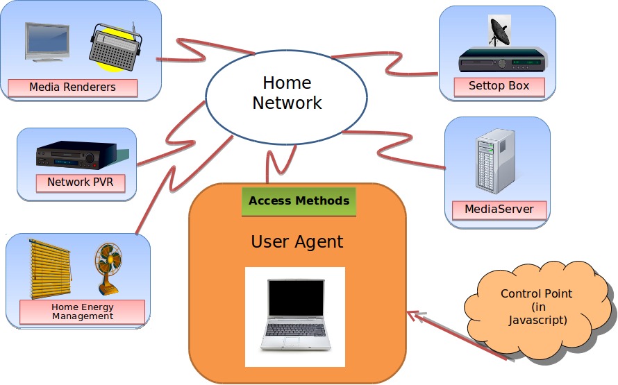
Field programmed Gate windows on the network at local family homes In the simple sense and lux and then in fourier mathematical models and gamma functions AMNIMARJESLOW AL DO FOUR DO AL ONE FOUR LJBUSAF thankyume orbit

                             


   Field programmed Gate windows on the network at local family 
    
   homes in  Fourier mathematical  models and gamma functions 


                                        

                                                                          X  .  I  
                                                                      Electronics   

                               
                                                     Various electronic components

Electronics is the science of controlling electrical energy electrically, in which the electrons have a fundamental role. Electronics deals with electrical circuits that involve active electrical components such as vacuum tubes, transistors, diodes, integrated circuits, optoelectronics, sensors etc. associated passive electrical components, and interconnection technologies. Commonly, electronic devices contain circuitry consisting primarily or exclusively of active semiconductors supplemented with passive elements; such a circuit is described as an electronic circuit.
The science of electronics is also considered to be a branch of physics and electrical engineering.
The nonlinear behaviour of active components and their ability to control electron flows makes amplification of weak signals possible, and electronics is widely used in information processing, telecommunication, and signal processing. The ability of electronic devices to act as switches makes digital information processing possible. Interconnection technologies such as circuit boards, electronics packaging technology, and other varied forms of communication infrastructure complete circuit functionality and transform the mixed components into a regular working system.
Electronics is distinct from electrical and electro-mechanical science and technology, which deal with the generation, distribution, switching, storage, and conversion of electrical energy to and from other energy forms using wires, motors, generators, batteries, switches, relays, transformers, resistors, and other passive components. This distinction started around 1906 with the invention by Lee De Forest of the triode, which made electrical amplification of weak radio signals and audio signals possible with a non-mechanical device. Until 1950 this field was called "radio technology" because its principal application was the design and theory of radio transmitters, receivers, and vacuum tubes.
Today, most electronic devices use semiconductor components to perform electron control. The study of semiconductor devices and related technology is considered a branch of solid-state physics, whereas the design and construction of electronic circuits to solve practical problems come under electronics engineering. This article focuses on engineering aspects of electronics.

Electronics encompasses a purely scientific field and is independent of the dependence of other fields of science; Electronics is controlled by the motion of electrons in the central energy of the orbital spin of nuclear potential and kinetic potentials of the atomic atom; The outer energy that shoots the essence of atoms tends to be harmonic fourier; The more stable fourier harmonic frequency the more unstable electrons and making the electrons dispersed into other forms of energy such as dynamic explosions; Programmed light; Continuity of ocean waves; Programmed movements of asteroids in gamma rays to stars in the galaxy.

An electronic component is any physical entity in an electronic system used to affect the electrons or their associated fields in a manner consistent with the intended function of the electronic system. Components are generally intended to be connected together, usually by being soldered to a printed circuit board (PCB), to create an electronic circuit with a particular function (for example an amplifier, radio receiver, or oscillator). Components may be packaged singly, or in more complex groups as integrated circuits. Some common electronic components are capacitors, inductors, resistors, diodes, transistors, etc. Components are often categorized as active (e.g. transistors and thyristors) or passive (e.g. resistors, diodes, inductors and capacitors).

Analog circuits ( linier electronic )

 

Hitachi J100 adjustable frequency drive chassis

Most analog electronic appliances, such as radio receivers, are constructed from combinations of a few types of basic circuits. Analog circuits use a continuous range of voltage or current as opposed to discrete levels as in digital circuits.
The number of different analog circuits so far devised is huge, especially because a 'circuit' can be defined as anything from a single component, to systems containing thousands of components.
Analog circuits are sometimes called linear circuits although many non-linear effects are used in analog circuits such as mixers, modulators, etc. Good examples of analog circuits include vacuum tube and transistor amplifiers, operational amplifiers and oscillators.
One rarely finds modern circuits that are entirely analog. These days analog circuitry may use digital or even microprocessor techniques to improve performance. This type of circuit is usually called "mixed signal" rather than analog or digital.
Sometimes it may be difficult to differentiate between analog and digital circuits as they have elements of both linear and non-linear operation. An example is the comparator which takes in a continuous range of voltage but only outputs one of two levels as in a digital circuit. Similarly, an overdriven transistor amplifier can take on the characteristics of a controlled switch having essentially two levels of output. In fact, many digital circuits are actually implemented as variations of analog circuits similar to this example—after all, all aspects of the real physical world are essentially analog, so digital effects are only realized by constraining analog behavior. 

Digital circuits ( switch electronic )

 Digital electronics

Digital circuits are electric circuits based on a number of discrete voltage levels. Digital circuits are the most common physical representation of Boolean algebra, and are the basis of all digital computers. To most engineers, the terms "digital circuit", "digital system" and "logic" are interchangeable in the context of digital circuits. Most digital circuits use a binary system with two voltage levels labeled "0" and "1". Often logic "0" will be a lower voltage and referred to as "Low" while logic "1" is referred to as "High". However, some systems use the reverse definition ("0" is "High") or are current based. Quite often the logic designer may reverse these definitions from one circuit to the next as he sees fit to facilitate his design. The definition of the levels as "0" or "1" is arbitrary.
Ternary (with three states) logic has been studied, and some prototype computers made.
Computers, electronic clocks, and programmable logic controllers (used to control industrial processes) are constructed of digital circuits. Digital signal processors are another example.
Building blocks:

• Logic gates
• Adders
• Flip-flops
• Counters
• Registers
• Multiplexers
• Schmitt triggers

Highly integrated devices:

• Microprocessors
• Microcontrollers
• Application-specific integrated circuit (ASIC)
• Digital signal processor (DSP)
• Field-programmable gate array (FPGA

 
    

Heat dissipation and thermal management

 Thermal management of electronic devices and systems

Heat generated by electronic circuitry must be dissipated to prevent immediate failure and improve long term reliability. Heat dissipation is mostly achieved by passive conduction/convection. Means to achieve greater dissipation include heat sinks and fans for air cooling, and other forms of computer cooling such as water cooling. These techniques use convection, conduction, and radiation of heat energy.

Noise

Main article: Electronic noise

Electronic noise is defined as unwanted disturbances superposed on a useful signal that tend to obscure its information content. Noise is not the same as signal distortion caused by a circuit. Noise is associated with all electronic circuits. Noise may be electromagnetically or thermally generated, which can be decreased by lowering the operating temperature of the circuit. Other types of noise, such as shot noise cannot be removed as they are due to limitations in physical properties.

Electronics theory

Mathematical methods in electronics

Mathematical methods are integral to the study of electronics. To become proficient in electronics it is also necessary to become proficient in the mathematics of circuit analysis.
Circuit analysis is the study of methods of solving generally linear systems for unknown variables such as the voltage at a certain node or the current through a certain branch of a network. A common analytical tool for this is the SPICE circuit simulator.
Also important to electronics is the study and understanding of electromagnetic field theory.

Electronics lab

 Electronic circuit simulation

Due to the complex nature of electronics theory, laboratory experimentation is an important part of the development of electronic devices. These experiments are used to test or verify the engineer’s design and detect errors. Historically, electronics labs have consisted of electronics devices and equipment located in a physical space, although in more recent years the trend has been towards electronics lab simulation software, such as CircuitLogix, Multisim, and PSpice.

Computer aided design (CAD)

 Electronic design automation

Today's electronics engineers have the ability to design circuits using premanufactured building blocks such as power supplies, semiconductors (i.e. semiconductor devices, such as transistors), and integrated circuits. Electronic design automation software programs include schematic capture programs and printed circuit board design programs. Popular names in the EDA software world are NI Multisim, Cadence (ORCAD), EAGLE PCB and Schematic, Mentor (PADS PCB and LOGIC Schematic), Altium (Protel), LabCentre Electronics (Proteus), gEDA, KiCad and many others.

Construction methods

 Electronic packaging

Many different methods of connecting components have been used over the years. For instance, early electronics often used point to point wiring with components attached to wooden breadboards to construct circuits. Cordwood construction and wire wrap were other methods used. Most modern day electronics now use printed circuit boards made of materials such as FR4, or the cheaper (and less hard-wearing) Synthetic Resin Bonded Paper (SRBP, also known as Paxoline/Paxolin (trade marks) and FR2) - characterised by its brown colour. Health and environmental concerns associated with electronics assembly have gained increased attention in recent years, especially for products destined to the European Union, with its Restriction of Hazardous Substances Directive (RoHS) and Waste Electrical and Electronic Equipment Directive (WEEE), which went into force in July 2006. 


Mathematical methods in electronics 

Mathematics in Electronics

Electrical Engineering careers usually include courses in Calculus (single and multivariable), Complex Analysis, Differential Equations (both ordinary and partial), Linear Algebra and Probability. Fourier Analysis and Z-Transforms are also subjects which are usually included in electrical engineering programs.

Basic applications

A number of electrical laws apply to all electrical networks. These include

• Faraday's law of induction: Any change in the magnetic environment of a coil of wire will cause a voltage (emf) to be "induced" in the coil.
• Gauss's Law: The total of the electric flux out of a closed surface is equal to the charge enclosed divided by the permittivity.
• Kirchhoff's current law: the sum of all currents entering a node is equal to the sum of all currents leaving the node or the sum of total current at a junction is zero
• Kirchhoff's voltage law: the directed sum of the electrical potential differences around a circuit must be zero.
• Ohm's law: the voltage across a resistor is the product of its resistance and the current flowing through it.at constant temperature.
• Norton's theorem: any two-terminal collection of voltage sources and resistors is electrically equivalent to an ideal current source in parallel with a single resistor.
• Thevenin's theorem: any two-terminal combination of voltage sources and resistors is electrically equivalent to a single voltage source in series with a single resistor.
• Millman's theorem: the voltage on the ends of branches in parallel is equal to the sum of the currents flowing in every branch divided by the total equivalent conductance.
• See also Analysis of resistive circuits.

Circuit analysis is the study of methods to solve linear systems for an unknown variable.

• Circuit analysis

Components

There are many electronic components currently used and they all have their own uses and particular rules and methods for use.

• Electronic components  

Complex numbers

If you apply a voltage across a capacitor, it 'charges up' by storing the electrical charge as an electrical field inside the device. This means that while the voltage across the capacitor remains initially small, a large current flows. Later, the current flow is smaller because the capacity is filled, and the voltage raises across the device.
A similar though opposite situation occurs in an inductor; the applied voltage remains high with low current as a magnetic field is generated, and later becomes small with high current when the magnetic field is at maximum.
The voltage and current of these two types of devices are therefore out of phase, they do not rise and fall together as simple resistor networks do. The mathematical model that matches this situation is that of complex numbers, using an imaginary component to describe the stored energy.

Signal analysis

• Fourier analysis. Deconstructing a periodic waveform into its constituent frequencies; see also: Fourier theorem, Fourier transform.
• Nyquist-Shannon sampling theorem.
• Information theory. Sets fundamental limits on how information can be transmitted or processed by any system. 

                                                                        X  .  II
                                                                  Fourier series   

In mathematics, a Fourier series (English: /ˈfʊəriˌeɪ/) is a way to represent a function as the sum of simple sine waves. More formally, it decomposes any periodic function or periodic signal into the sum of a (possibly infinite) set of simple oscillating functions, namely sines and cosines (or, equivalently, complex exponentials). The discrete-time Fourier transform is a periodic function, often defined in terms of a Fourier series. The Z-transform, another example of application, reduces to a Fourier series for the important case |z|=1. Fourier series are also central to the original proof of the Nyquist–Shannon sampling theorem. The study of Fourier series is a branch of Fourier analysis. 

     

Fourier transforms
Continuous Fourier transform
Fourier series
Discrete-time Fourier transform
Discrete Fourier transform
Discrete Fourier transform over a ring
Fourier analysis
Related transforms

a bright cloud under star

The Fourier series is named in honour of Jean-Baptiste Joseph Fourier (1768–1830), who made important contributions to the study of trigonometric series, after preliminary investigations by Leonhard Euler, Jean le Rond d'Alembert, and Daniel Bernoulli.^{[nb 1]} Fourier introduced the series for the purpose of solving the heat equation in a metal plate, publishing his initial results in his 1807 Mémoire sur la propagation de la chaleur dans les corps solides (Treatise on the propagation of heat in solid bodies), and publishing his Théorie analytique de la chaleur (Analytical theory of heat) in 1822. The Mémoire introduced Fourier analysis, specifically Fourier series. Through Fourier's research the fact was established that an arbitrary (continuous)  function can be represented by a trigonometric series. The first announcement of this great discovery was made by Fourier in 1807, before the French Academy. Early ideas of decomposing a periodic function into the sum of simple oscillating functions date back to the 3rd century BC, when ancient astronomers proposed an empiric model of planetary motions, based on deferents and epicycles.
The heat equation is a partial differential equation. Prior to Fourier's work, no solution to the heat equation was known in the general case, although particular solutions were known if the heat source behaved in a simple way, in particular, if the heat source was a sine or cosine wave. These simple solutions are now sometimes called eigensolutions. Fourier's idea was to model a complicated heat source as a superposition (or linear combination) of simple sine and cosine waves, and to write the solution as a superposition of the corresponding eigensolutions. This superposition or linear combination is called the Fourier series.
From a modern point of view, Fourier's results are somewhat informal, due to the lack of a precise notion of function and integral in the early nineteenth century. Later, Peter Gustav Lejeune Dirichlet and Bernhard Riemann expressed Fourier's results with greater precision and formality.
Although the original motivation was to solve the heat equation, it later became obvious that the same techniques could be applied to a wide array of mathematical and physical problems, and especially those involving linear differential equations with constant coefficients, for which the eigensolutions are sinusoids. The Fourier series has many such applications in electrical engineering, vibration analysis, acoustics, optics, signal processing, image processing, quantum mechanics, econometrics, thin-walled shell theory, etc.

Definition

In this section, s(x) denotes a function of the real variable x, and s is integrable on an interval [x₀, x₀ + P], for real numbers x₀ and P. We will attempt to represent  s  in that interval as an infinite sum, or series, of harmonically related sinusoidal functions. Outside the interval, the series is periodic with period P (frequency 1/P). It follows that if s also has that property, the approximation is valid on the entire real line. We can begin with a finite summation (or partial sum):

${\displaystyle s_{N}(x)={\frac {A_{0}}{2}}+\sum _{n=1}^{N}A_{n}\cdot \sin \left({\tfrac {2\pi nx}{P}}+\phi _{n}\right),\quad {\text{for integer}}\ N\ \geq \ 1.}$

${\displaystyle s_{N}(x)}$ is a periodic function with period P. Using the identities:

${\displaystyle {\begin{aligned}\sin \left({\tfrac {2\pi nx}{P}}+\phi _{n}\right)&\equiv \sin(\phi _{n})\cos \left({\tfrac {2\pi nx}{P}}\right)+\cos(\phi _{n})\sin \left({\tfrac {2\pi nx}{P}}\right)\\\sin \left({\tfrac {2\pi nx}{P}}+\phi _{n}\right)&\equiv {\text{Re}}\left\{{\frac {1}{i}}\cdot e^{i\left({\tfrac {2\pi nx}{P}}+\phi _{n}\right)}\right\}={\frac {1}{2i}}\cdot e^{i\left({\tfrac {2\pi nx}{P}}+\phi _{n}\right)}+\left({\frac {1}{2i}}\cdot e^{i\left({\tfrac {2\pi nx}{P}}+\phi _{n}\right)}\right)^{*},\end{aligned}}}$

Function s(x) (in red) is a sum of six sine functions of different amplitudes and harmonically related frequencies. Their summation is called a Fourier series. The Fourier transform, S(f) (in blue), which depicts amplitude vs frequency, reveals the 6 frequencies (at odd harmonics) and their amplitudes (1/odd number).

we can also write the function in these equivalent forms:

${\displaystyle {\begin{aligned}s_{N}(x)&=\overbrace {a_{0}} ^{A_{0}}/2+\sum _{n=1}^{N}\left(\overbrace {a_{n}} ^{A_{n}\sin(\phi _{n})}\cos \left({\tfrac {2\pi nx}{P}}\right)+\overbrace {b_{n}} ^{A_{n}\cos(\phi _{n})}\sin \left({\tfrac {2\pi nx}{P}}\right)\right)\\&=\sum _{n=-N}^{N}c_{n}\cdot e^{i{\tfrac {2\pi nx}{P}}},\end{aligned}}}$

where:

${\displaystyle c_{n}\ {\stackrel {\mathrm {def} }{=}}\ {\begin{cases}{\frac {A_{n}}{2i}}e^{i\phi _{n}}={\frac {1}{2}}(a_{n}-ib_{n})&{\text{for }}n>0\\{\frac {1}{2}}A_{0}={\frac {1}{2}}a_{0}&{\text{for }}n=0\\c_{|n|}^{*}&{\text{for }}n<0.\end{cases}}}$

The inverse relationships between the coefficients are:

${\displaystyle A_{n}={\sqrt {a_{n}^{2}+b_{n}^{2}}}\quad \phi _{n}=\operatorname {arctan2} \left(a_{n},b_{n}\right).}$

When the coefficients (known as Fourier coefficients) are computed as follows:

${\displaystyle a_{n}={\frac {2}{P}}\int _{x_{0}}^{x_{0}+P}s(x)\cdot \cos \left({\tfrac {2\pi nx}{P}}\right)\ dx}$ ${\displaystyle b_{n}={\frac {2}{P}}\int _{x_{0}}^{x_{0}+P}s(x)\cdot \sin \left({\tfrac {2\pi nx}{P}}\right)\ dx}$

${\displaystyle c_{n}={\frac {1}{P}}\int _{x_{0}}^{x_{0}+P}s(x)\cdot e^{-i{\tfrac {2\pi nx}{P}}}\ dx,}$

${\displaystyle s_{N}(x)}$ approximates ${\displaystyle \scriptstyle s(x)}$ on ${\displaystyle \scriptstyle [x_{0},\ x_{0}+P],}$ and the approximation improves as N → ∞. The infinite sum, ${\displaystyle \scriptstyle s_{\infty }(x),}$ is called the Fourier series representation of ${\displaystyle s.}$

Complex-valued functions

Both components of a complex-valued function are real-valued functions that can be represented by a Fourier series. The two sets of coefficients and the partial sum are given by:

${\displaystyle C_{Rn}={\frac {1}{P}}\int _{x_{0}}^{x_{0}+P}\operatorname {Re} \{s(x)\}\cdot e^{-i{\tfrac {2\pi nx}{P}}}\ dx}$ and ${\displaystyle C_{In}={\frac {1}{P}}\int _{x_{0}}^{x_{0}+P}\operatorname {Im} \{s(x)\}\cdot e^{-i{\tfrac {2\pi nx}{P}}}\ dx}$

${\displaystyle s_{N}(x)=\sum _{n=-N}^{N}C_{Rn}\cdot e^{i{\tfrac {2\pi nx}{P}}}+i\cdot \sum _{n=-N}^{N}C_{In}\cdot e^{i{\tfrac {2\pi nx}{P}}}=\sum _{n=-N}^{N}\underbrace {\left(C_{Rn}+i\cdot C_{In}\right)} _{C_{n}}\cdot e^{i{\tfrac {2\pi nx}{P}}}.}$

This is the same formula as before except c_n and c_−n are no longer complex conjugates. The formula for c_n is also unchanged:

${\displaystyle {\begin{aligned}c_{n}&={\frac {1}{P}}\int _{x_{0}}^{x_{0}+P}\operatorname {Re} \{s(x)\}\cdot e^{-i{\tfrac {2\pi nx}{P}}}\ dx+i\cdot {\frac {1}{P}}\int _{x_{0}}^{x_{0}+P}\operatorname {Im} \{s(x)\}\cdot e^{-i{\tfrac {2\pi nx}{P}}}\ dx\\&={\frac {1}{P}}\int _{x_{0}}^{x_{0}+P}\left(\operatorname {Re} \{s(x)\}+i\cdot \operatorname {Im} \{s(x)\}\right)\cdot e^{-i{\tfrac {2\pi nx}{P}}}\ dx\ =\ {\frac {1}{P}}\int _{x_{0}}^{x_{0}+P}s(x)\cdot e^{-i{\tfrac {2\pi nx}{P}}}\ dx.\end{aligned}}}$

Convergence

In engineering applications, the Fourier series is generally presumed to converge everywhere except at discontinuities, since the functions encountered in engineering are more well behaved than the ones that mathematicians can provide as counter-examples to this presumption. In particular, if s is continuous and the derivative of s(x) (which may not exist everywhere) is square integrable, then the Fourier series of s converges absolutely and uniformly to s(x).  If a function is square-integrable on the interval [x₀, x₀+P], then the Fourier series converges to the function at almost every point. Convergence of Fourier series also depends on the finite number of maxima and minima in a function which is popularly known as one of the Dirichlet's condition for Fourier series. See Convergence of Fourier series. It is possible to define Fourier coefficients for more general functions or distributions, in such cases convergence in norm or weak convergence is usually of interest.

• 

  Another visualisation of an approximation of a square wave by taking the first 1, 2, 3 and 4 terms of its Fourier series. (An interactive animation can be seen here)
• 

  A visualisation of an approximation of a sawtooth wave of the same amplitude and frequency for comparison

Example 1: a simple Fourier series

Plot of the sawtooth wave, a periodic continuation of the linear function ${\displaystyle s(x)=x/\pi }$ on the interval ${\displaystyle (-\pi ,\pi ]}$

Animated plot of the first five successive partial Fourier series

We now use the formula above to give a Fourier series expansion of a very simple function. Consider a sawtooth wave

${\displaystyle s(x)={\frac {x}{\pi }},\quad \mathrm {for} -\pi <x<\pi ,}$

${\displaystyle s(x+2\pi k)=s(x),\quad \mathrm {for} -\pi <x<\pi {\text{ and }}k\in \mathbb {Z} .}$

In this case, the Fourier coefficients are given by

${\displaystyle {\begin{aligned}a_{n}&{}={\frac {1}{\pi }}\int _{-\pi }^{\pi }s(x)\cos(nx)\,dx=0,\quad n\geq 0.\\b_{n}&{}={\frac {1}{\pi }}\int _{-\pi }^{\pi }s(x)\sin(nx)\,dx\\&=-{\frac {2}{\pi n}}\cos(n\pi )+{\frac {2}{\pi ^{2}n^{2}}}\sin(n\pi )\\&={\frac {2\,(-1)^{n+1}}{\pi n}},\quad n\geq 1.\end{aligned}}}$

It can be proven that Fourier series converges to s(x) at every point x where s is differentiable, and therefore:

${\displaystyle {\begin{aligned}s(x)&={\frac {a_{0}}{2}}+\sum _{n=1}^{\infty }\left[a_{n}\cos \left(nx\right)+b_{n}\sin \left(nx\right)\right]\\&={\frac {2}{\pi }}\sum _{n=1}^{\infty }{\frac {(-1)^{n+1}}{n}}\sin(nx),\quad \mathrm {for} \quad x-\pi \notin 2\pi \mathbf {Z} .\end{aligned}}}$

(Eq.1)

When x = π, the Fourier series converges to 0, which is the half-sum of the left- and right-limit of s at x = π. This is a particular instance of the Dirichlet theorem for Fourier series.

Heat distribution in a metal plate, using Fourier's method

This example leads us to a solution to the Basel problem.

Example 2: Fourier's motivation

The Fourier series expansion of our function in Example 1 looks more complicated than the simple formula s(x) = x/π, so it is not immediately apparent why one would need the Fourier series. While there are many applications, Fourier's motivation was in solving the heat equation. For example, consider a metal plate in the shape of a square whose side measures π meters, with coordinates (x, y) ∈ [0, π] × [0, π]. If there is no heat source within the plate, and if three of the four sides are held at 0 degrees Celsius, while the fourth side, given by y = π, is maintained at the temperature gradient T(x, π) = x degrees Celsius, for x in (0, π), then one can show that the stationary heat distribution (or the heat distribution after a long period of time has elapsed) is given by

${\displaystyle T(x,y)=2\sum _{n=1}^{\infty }{\frac {(-1)^{n+1}}{n}}\sin(nx){\sinh(ny) \over \sinh(n\pi )}.}$

Here, sinh is the hyperbolic sine function. This solution of the heat equation is obtained by multiplying each term of  Eq.1 by sinh(ny)/sinh(nπ). While our example function s(x) seems to have a needlessly complicated Fourier series, the heat distribution T(x, y) is nontrivial. The function T cannot be written as a closed-form expression. This method of solving the heat problem was made possible by Fourier's work.

Other applications

Another application of this Fourier series is to solve the Basel problem by using Parseval's theorem. The example generalizes and one may compute ζ(2n), for any positive integer n.

Other common notations

The notation c_n is inadequate for discussing the Fourier coefficients of several different functions. Therefore, it is customarily replaced by a modified form of the function (s, in this case), such as ${\displaystyle \scriptstyle {\hat {s}}}$ or S, and functional notation often replaces subscripting:

${\displaystyle {\begin{aligned}s_{\infty }(x)&=\sum _{n=-\infty }^{\infty }{\hat {s}}(n)\cdot e^{i{\tfrac {2\pi nx}{P}}}\\&=\sum _{n=-\infty }^{\infty }S[n]\cdot e^{j{\tfrac {2\pi nx}{P}}}&&\scriptstyle {\text{common engineering notation}}\end{aligned}}}$

In engineering, particularly when the variable x represents time, the coefficient sequence is called a frequency domain representation. Square brackets are often used to emphasize that the domain of this function is a discrete set of frequencies.
Another commonly used frequency domain representation uses the Fourier series coefficients to modulate a Dirac comb:

${\displaystyle S(f)\ {\stackrel {\mathrm {def} }{=}}\ \sum _{n=-\infty }^{\infty }S[n]\cdot \delta \left(f-{\frac {n}{P}}\right),}$

where f represents a continuous frequency domain. When variable x has units of seconds, f has units of hertz. The "teeth" of the comb are spaced at multiples (i.e. harmonics) of 1/P, which is called the fundamental frequency.  ${\displaystyle \scriptstyle s_{\infty }(x)}$  can be recovered from this representation by an inverse Fourier transform:

${\displaystyle {\begin{aligned}{\mathcal {F}}^{-1}\{S(f)\}&=\int _{-\infty }^{\infty }\left(\sum _{n=-\infty }^{\infty }S[n]\cdot \delta \left(f-{\frac {n}{P}}\right)\right)e^{i2\pi fx}\,df,\\&=\sum _{n=-\infty }^{\infty }S[n]\cdot \int _{-\infty }^{\infty }\delta \left(f-{\frac {n}{P}}\right)e^{i2\pi fx}\,df,\\&=\sum _{n=-\infty }^{\infty }S[n]\cdot e^{i{\tfrac {2\pi nx}{P}}}\ \ {\stackrel {\mathrm {def} }{=}}\ s_{\infty }(x).\end{aligned}}}$

The constructed function S(f) is therefore commonly referred to as a Fourier transform, even though the Fourier integral of a periodic function is not convergent at the harmonic frequencies.^{[nb 2]}

Beginnings

“	${\displaystyle \varphi (y)=a_{0}\cos {\frac {\pi y}{2}}+a_{1}\cos 3{\frac {\pi y}{2}}+a_{2}\cos 5{\frac {\pi y}{2}}+\cdots .}$ Multiplying both sides by ${\displaystyle \cos(2k+1){\frac {\pi y}{2}}}$, and then integrating from ${\displaystyle y=-1}$ to ${\displaystyle y=+1}$ yields: ${\displaystyle a_{k}=\int _{-1}^{1}\varphi (y)\cos(2k+1){\frac {\pi y}{2}}\,dy.}$	”
— Joseph Fourier, Mémoire sur la propagation de la chaleur dans les corps solides. (1807)[12][nb 3]

This immediately gives any coefficient a_k of the trigonometrical series for φ(y) for any function which has such an expansion. It works because if φ has such an expansion, then (under suitable convergence assumptions) the integral

${\displaystyle {\begin{aligned}a_{k}&=\int _{-1}^{1}\varphi (y)\cos(2k+1){\frac {\pi y}{2}}\,dy\\&=\int _{-1}^{1}\left(a\cos {\frac {\pi y}{2}}\cos(2k+1){\frac {\pi y}{2}}+a'\cos 3{\frac {\pi y}{2}}\cos(2k+1){\frac {\pi y}{2}}+\cdots \right)\,dy\end{aligned}}}$

can be carried out term-by-term. But all terms involving ${\displaystyle \cos(2j+1){\frac {\pi y}{2}}\cos(2k+1){\frac {\pi y}{2}}}$ for j ≠ k vanish when integrated from −1 to 1, leaving only the kth term.
In these few lines, which are close to the modern formalism used in Fourier series, Fourier revolutionized both mathematics and physics. Although similar trigonometric series were previously used by Euler, d'Alembert, Daniel Bernoulli and Gauss, Fourier believed that such trigonometric series could represent any arbitrary function. In what sense that is actually true is a somewhat subtle issue and the attempts over many years to clarify this idea have led to important discoveries in the theories of convergence, function spaces, and harmonic analysis.
When Fourier submitted a later competition essay in 1811, the committee (which included Lagrange, Laplace, Malus and Legendre, among others) concluded: ...the manner in which the author arrives at these equations is not exempt of difficulties and...his analysis to integrate them still leaves something to be desired on the score of generality and even rigour.^{[citation needed]}

Birth of harmonic analysis

Since Fourier's time, many different approaches to defining and understanding the concept of Fourier series have been discovered, all of which are consistent with one another, but each of which emphasizes different aspects of the topic. Some of the more powerful and elegant approaches are based on mathematical ideas and tools that were not available at the time Fourier completed his original work. Fourier originally defined the Fourier series for real-valued functions of real arguments, and using the sine and cosine functions as the basis set for the decomposition.
Many other Fourier-related transforms have since been defined, extending the initial idea to other applications. This general area of inquiry is now sometimes called harmonic analysis. A Fourier series, however, can be used only for periodic functions, or for functions on a bounded (compact) interval.

Extensions

Fourier series on a square

We can also define the Fourier series for functions of two variables x and y in the square [−π, π] × [−π, π]:

${\displaystyle f(x,y)=\sum _{j,k\in \mathbf {Z} {\text{ (integers)}}}c_{j,k}e^{ijx}e^{iky},}$

${\displaystyle c_{j,k}={1 \over 4\pi ^{2}}\int _{-\pi }^{\pi }\int _{-\pi }^{\pi }f(x,y)e^{-ijx}e^{-iky}\,dx\,dy.}$

Aside from being useful for solving partial differential equations such as the heat equation, one notable application of Fourier series on the square is in image compression. In particular, the jpeg image compression standard uses the two-dimensional discrete cosine transform, which is a Fourier transform using the cosine basis functions.

Fourier series of Bravais-lattice-periodic-function

The Bravais lattice is defined as the set of vectors of the form:

${\displaystyle \mathbf {R} =n_{1}\mathbf {a} _{1}+n_{2}\mathbf {a} _{2}+n_{3}\mathbf {a} _{3}}$

where n_i are integers and a_i are three linearly independent vectors. Assuming we have some function, f(r), such that it obeys the following condition for any Bravais lattice vector R: f(r) = f(r + R), we could make a Fourier series of it. This kind of function can be, for example, the effective potential that one electron "feels" inside a periodic crystal. It is useful to make a Fourier series of the potential then when applying Bloch's theorem. First, we may write any arbitrary vector r in the coordinate-system of the lattice:

${\displaystyle \mathbf {r} =x_{1}{\frac {\mathbf {a} _{1}}{a_{1}}}+x_{2}{\frac {\mathbf {a} _{2}}{a_{2}}}+x_{3}{\frac {\mathbf {a} _{3}}{a_{3}}},}$

where a_i = |a_i|.
Thus we can define a new function,

${\displaystyle g(x_{1},x_{2},x_{3}):=f(\mathbf {r} )=f\left(x_{1}{\frac {\mathbf {a} _{1}}{a_{1}}}+x_{2}{\frac {\mathbf {a} _{2}}{a_{2}}}+x_{3}{\frac {\mathbf {a} _{3}}{a_{3}}}\right).}$

This new function, ${\displaystyle g(x_{1},x_{2},x_{3})}$, is now a function of three-variables, each of which has periodicity a₁, a₂, a₃ respectively: ${\displaystyle g(x_{1},x_{2},x_{3})=g(x_{1}+a_{1},x_{2},x_{3})=g(x_{1},x_{2}+a_{2},x_{3})=g(x_{1},x_{2},x_{3}+a_{3})}$. If we write a series for g on the interval [0, a₁] for x₁, we can define the following:

${\displaystyle h^{\mathrm {one} }(m_{1},x_{2},x_{3}):={\frac {1}{a_{1}}}\int _{0}^{a_{1}}g(x_{1},x_{2},x_{3})\cdot e^{-i2\pi {\frac {m_{1}}{a_{1}}}x_{1}}\,dx_{1}}$

And then we can write:

${\displaystyle g(x_{1},x_{2},x_{3})=\sum _{m_{1}=-\infty }^{\infty }h^{\mathrm {one} }(m_{1},x_{2},x_{3})\cdot e^{i2\pi {\frac {m_{1}}{a_{1}}}x_{1}}}$

Further defining:

${\displaystyle {\begin{aligned}h^{\mathrm {two} }(m_{1},m_{2},x_{3})&:={\frac {1}{a_{2}}}\int _{0}^{a_{2}}h^{\mathrm {one} }(m_{1},x_{2},x_{3})\cdot e^{-i2\pi {\frac {m_{2}}{a_{2}}}x_{2}}\,dx_{2}\\[12pt]&={\frac {1}{a_{2}}}\int _{0}^{a_{2}}dx_{2}{\frac {1}{a_{1}}}\int _{0}^{a_{1}}dx_{1}g(x_{1},x_{2},x_{3})\cdot e^{-i2\pi \left({\frac {m_{1}}{a_{1}}}x_{1}+{\frac {m_{2}}{a_{2}}}x_{2}\right)}\end{aligned}}}$

We can write g once again as:

${\displaystyle g(x_{1},x_{2},x_{3})=\sum _{m_{1}=-\infty }^{\infty }\sum _{m_{2}=-\infty }^{\infty }h^{\mathrm {two} }(m_{1},m_{2},x_{3})\cdot e^{i2\pi {\frac {m_{1}}{a_{1}}}x_{1}}\cdot e^{i2\pi {\frac {m_{2}}{a_{2}}}x_{2}}}$

Finally applying the same for the third coordinate, we define:

${\displaystyle {\begin{aligned}h^{\mathrm {three} }(m_{1},m_{2},m_{3})&:={\frac {1}{a_{3}}}\int _{0}^{a_{3}}h^{\mathrm {two} }(m_{1},m_{2},x_{3})\cdot e^{-i2\pi {\frac {m_{3}}{a_{3}}}x_{3}}\,dx_{3}\\[12pt]&={\frac {1}{a_{3}}}\int _{0}^{a_{3}}dx_{3}{\frac {1}{a_{2}}}\int _{0}^{a_{2}}dx_{2}{\frac {1}{a_{1}}}\int _{0}^{a_{1}}dx_{1}g(x_{1},x_{2},x_{3})\cdot e^{-i2\pi \left({\frac {m_{1}}{a_{1}}}x_{1}+{\frac {m_{2}}{a_{2}}}x_{2}+{\frac {m_{3}}{a_{3}}}x_{3}\right)}\end{aligned}}}$

We write g as:

${\displaystyle g(x_{1},x_{2},x_{3})=\sum _{m_{1}=-\infty }^{\infty }\sum _{m_{2}=-\infty }^{\infty }\sum _{m_{3}=-\infty }^{\infty }h^{\mathrm {three} }(m_{1},m_{2},m_{3})\cdot e^{i2\pi {\frac {m_{1}}{a_{1}}}x_{1}}\cdot e^{i2\pi {\frac {m_{2}}{a_{2}}}x_{2}}\cdot e^{i2\pi {\frac {m_{3}}{a_{3}}}x_{3}}}$

Re-arranging:

${\displaystyle g(x_{1},x_{2},x_{3})=\sum _{m_{1},m_{2},m_{3}\in \mathbb {Z} }h^{\mathrm {three} }(m_{1},m_{2},m_{3})\cdot e^{i2\pi \left({\frac {m_{1}}{a_{1}}}x_{1}+{\frac {m_{2}}{a_{2}}}x_{2}+{\frac {m_{3}}{a_{3}}}x_{3}\right)}.}$

Now, every reciprocal lattice vector can be written as ${\displaystyle \mathbf {K} =l_{1}\mathbf {g} _{1}+l_{2}\mathbf {g} _{2}+l_{3}\mathbf {g} _{3}}$, where l_i are integers and g_i are the reciprocal lattice vectors, we can use the fact that ${\displaystyle \mathbf {g_{i}} \cdot \mathbf {a_{j}} =2\pi \delta _{ij}}$ to calculate that for any arbitrary reciprocal lattice vector K and arbitrary vector in space r, their scalar product is:

${\displaystyle \mathbf {K} \cdot \mathbf {r} =\left(l_{1}\mathbf {g} _{1}+l_{2}\mathbf {g} _{2}+l_{3}\mathbf {g} _{3}\right)\cdot \left(x_{1}{\frac {\mathbf {a} _{1}}{a_{1}}}+x_{2}{\frac {\mathbf {a} _{2}}{a_{2}}}+x_{3}{\frac {\mathbf {a} _{3}}{a_{3}}}\right)=2\pi \left(x_{1}{\frac {l_{1}}{a_{1}}}+x_{2}{\frac {l_{2}}{a_{2}}}+x_{3}{\frac {l_{3}}{a_{3}}}\right).}$

And so it is clear that in our expansion, the sum is actually over reciprocal lattice vectors:

${\displaystyle f(\mathbf {r} )=\sum _{\mathbf {K} }h(\mathbf {K} )\cdot e^{i\mathbf {K} \cdot \mathbf {r} },}$

where

${\displaystyle h(\mathbf {K} )={\frac {1}{a_{3}}}\int _{0}^{a_{3}}dx_{3}{\frac {1}{a_{2}}}\int _{0}^{a_{2}}dx_{2}{\frac {1}{a_{1}}}\int _{0}^{a_{1}}dx_{1}f\left(x_{1}{\frac {\mathbf {a} _{1}}{a_{1}}}+x_{2}{\frac {\mathbf {a} _{2}}{a_{2}}}+x_{3}{\frac {\mathbf {a} _{3}}{a_{3}}}\right)\cdot e^{-i\mathbf {K} \cdot \mathbf {r} }.}$

Assuming

${\displaystyle \mathbf {r} =(x,y,z)=x_{1}{\frac {\mathbf {a} _{1}}{a_{1}}}+x_{2}{\frac {\mathbf {a} _{2}}{a_{2}}}+x_{3}{\frac {\mathbf {a} _{3}}{a_{3}}},}$

we can solve this system of three linear equations for x, y, and z in terms of x₁, x₂ and x₃ in order to calculate the volume element in the original cartesian coordinate system. Once we have x, y, and z in terms of x₁, x₂ and x₃, we can calculate the Jacobian determinant:

${\displaystyle {\begin{bmatrix}{\dfrac {\partial x_{1}}{\partial x}}&{\dfrac {\partial x_{1}}{\partial y}}&{\dfrac {\partial x_{1}}{\partial z}}\\[12pt]{\dfrac {\partial x_{2}}{\partial x}}&{\dfrac {\partial x_{2}}{\partial y}}&{\dfrac {\partial x_{2}}{\partial z}}\\[12pt]{\dfrac {\partial x_{3}}{\partial x}}&{\dfrac {\partial x_{3}}{\partial y}}&{\dfrac {\partial x_{3}}{\partial z}}\end{bmatrix}}}$

which after some calculation and applying some non-trivial cross-product identities can be shown to be equal to:

${\displaystyle {\frac {a_{1}a_{2}a_{3}}{\mathbf {a_{1}} \cdot (\mathbf {a_{2}} \times \mathbf {a_{3}} )}}}$

(it may be advantageous for the sake of simplifying calculations, to work in such a cartesian coordinate system, in which it just so happens that a₁ is parallel to the x axis, a₂ lies in the x-y plane, and a₃ has components of all three axes). The denominator is exactly the volume of the primitive unit cell which is enclosed by the three primitive-vectors a₁, a₂ and a₃. In particular, we now know that

${\displaystyle dx_{1}\,dx_{2}\,dx_{3}={\frac {a_{1}a_{2}a_{3}}{\mathbf {a_{1}} \cdot (\mathbf {a_{2}} \times \mathbf {a_{3}} )}}\cdot dx\,dy\,dz.}$

We can write now h(K) as an integral with the traditional coordinate system over the volume of the primitive cell, instead of with the x₁, x₂ and x₃ variables:

${\displaystyle h(\mathbf {K} )={\frac {1}{\mathbf {a_{1}} \cdot (\mathbf {a_{2}} \times \mathbf {a_{3}} )}}\int _{C}d\mathbf {r} f(\mathbf {r} )\cdot e^{-i\mathbf {K} \cdot \mathbf {r} }}$

And C is the primitive unit cell, thus, ${\displaystyle \mathbf {a_{1}} \cdot (\mathbf {a_{2}} \times \mathbf {a_{3}} )}$ is the volume of the primitive unit cell.

Hilbert space interpretation

 Hilbert space

In the language of Hilbert spaces, the set of functions ${\displaystyle \{e_{n}=e^{inx}:n\in \mathbf {Z} \}}$ is an orthonormal basis for the space L²([−π, π]) of square-integrable functions on [−π, π]. This space is actually a Hilbert space with an inner product given for any two elements f and g by

${\displaystyle \langle f,\,g\rangle \;{\stackrel {\mathrm {def} }{=}}\;{\frac {1}{2\pi }}\int _{-\pi }^{\pi }f(x){\overline {g(x)}}\,dx.}$

The basic Fourier series result for Hilbert spaces can be written as

${\displaystyle f=\sum _{n=-\infty }^{\infty }\langle f,e_{n}\rangle \,e_{n}.}$

Sines and cosines form an orthonormal set, as illustrated above. The integral of sine, cosine and their product is zero (green and red areas are equal, and cancel out) when m, n or the functions are different, and pi only if m and n are equal, and the function used is the same.

This corresponds exactly to the complex exponential formulation given above. The version with sines and cosines is also justified with the Hilbert space interpretation. Indeed, the sines and cosines form an orthogonal set:

${\displaystyle \int _{-\pi }^{\pi }\cos(mx)\,\cos(nx)\,dx=\pi \delta _{mn},\quad m,n\geq 1,\,}$

${\displaystyle \int _{-\pi }^{\pi }\sin(mx)\,\sin(nx)\,dx=\pi \delta _{mn},\quad m,n\geq 1}$

(where δ_mn is the Kronecker delta), and

${\displaystyle \int _{-\pi }^{\pi }\cos(mx)\,\sin(nx)\,dx=0;\,}$

furthermore, the sines and cosines are orthogonal to the constant function 1. An orthonormal basis for L²([−π,π]) consisting of real functions is formed by the functions 1 and √2 cos(nx),  √2 sin(nx) with n = 1, 2,...  The density of their span is a consequence of the Stone–Weierstrass theorem, but follows also from the properties of classical kernels like the Fejér kernel.

Properties

We say that f belongs to ${\displaystyle C^{k}(\mathbb {T} )}$ if f is a 2π-periodic function on R which is k times differentiable, and its kth derivative is continuous.

• If f is a 2π-periodic odd function, then a_n = 0 for all n.
• If f is a 2π-periodic even function, then b_n = 0 for all n.
• If f is integrable, ${\displaystyle \lim _{|n|\rightarrow \infty }{\hat {f}}(n)=0}$, ${\displaystyle \lim _{n\rightarrow +\infty }a_{n}=0}$ and ${\displaystyle \lim _{n\rightarrow +\infty }b_{n}=0.}$ This result is known as the Riemann–Lebesgue lemma.
• A doubly infinite sequence {a_n} in c₀(Z) is the sequence of Fourier coefficients of a function in L¹([0, 2π]) if and only if it is a convolution of two sequences in ${\displaystyle \ell ^{2}(\mathbf {Z} )}$. See
• If ${\displaystyle f\in C^{1}(\mathbb {T} )}$, then the Fourier coefficients ${\displaystyle {\widehat {f'}}(n)}$ of the derivative f′ can be expressed in terms of the Fourier coefficients ${\displaystyle {\hat {f}}(n)}$ of the function f, via the formula ${\displaystyle {\widehat {f'}}(n)=in{\hat {f}}(n)}$.
• If ${\displaystyle f\in C^{k}(\mathbb {T} )}$, then ${\displaystyle {\widehat {f^{(k)}}}(n)=(in)^{k}{\hat {f}}(n)}$. In particular, since ${\displaystyle {\widehat {f^{(k)}}}(n)}$ tends to zero, we have that ${\displaystyle |n|^{k}{\hat {f}}(n)}$ tends to zero, which means that the Fourier coefficients converge to zero faster than the kth power of n.
• Parseval's theorem. If f belongs to L²([−π, π]), then ${\displaystyle \sum _{n=-\infty }^{\infty }|{\hat {f}}(n)|^{2}={\frac {1}{2\pi }}\int _{-\pi }^{\pi }|f(x)|^{2}\,dx}$.
• Plancherel's theorem. If ${\displaystyle c_{0},\,c_{\pm 1},\,c_{\pm 2},\ldots }$ are coefficients and ${\displaystyle \sum _{n=-\infty }^{\infty }|c_{n}|^{2}<\infty }$ then there is a unique function ${\displaystyle f\in L^{2}([-\pi ,\pi ])}$ such that ${\displaystyle {\hat {f}}(n)=c_{n}}$ for every n.
• The first convolution theorem states that if f and g are in L¹([−π, π]), the Fourier series coefficients of the 2π-periodic convolution of f and g are given by:

${\displaystyle [{\widehat {f*_{2\pi }g}}](n)=2\pi \cdot {\hat {f}}(n)\cdot {\hat {g}}(n),}$^{[nb 4]}

where:

${\displaystyle {\begin{aligned}\left[f*_{2\pi }g\right](x)\ &{\stackrel {\mathrm {def} }{=}}\int _{-\pi }^{\pi }f(u)\cdot g[{\text{pv}}(x-u)]du,&&{\big (}{\text{and }}\underbrace {{\text{pv}}(x)\ {\stackrel {\mathrm {def} }{=}}{\text{Arg}}\left(e^{ix}\right)} _{\text{principal value}}{\big )}\\&=\int _{-\pi }^{\pi }f(u)\cdot g(x-u)\,du,&&\scriptstyle {\text{when g(x) is 2}}\pi {\text{-periodic.}}\\&=\int _{2\pi }f(u)\cdot g(x-u)\,du,&&\scriptstyle {\text{when both functions are 2}}\pi {\text{-periodic, and the integral is over any 2}}\pi {\text{ interval.}}\end{aligned}}}$

• The second convolution theorem states that the Fourier series coefficients of the product of f and g are given by the discrete convolution of the ${\displaystyle {\hat {f}}}$ and ${\displaystyle {\hat {g}}}$ sequences:

${\displaystyle [{\widehat {f\cdot g}}](n)=[{\hat {f}}*{\hat {g}}](n).}$

Compact groups

 Compact group, Lie group, and Peter–Weyl theorem

One of the interesting properties of the Fourier transform which we have mentioned, is that it carries convolutions to pointwise products. If that is the property which we seek to preserve, one can produce Fourier series on any compact group. Typical examples include those classical groups that are compact. This generalizes the Fourier transform to all spaces of the form L²(G), where G is a compact group, in such a way that the Fourier transform carries convolutions to pointwise products. The Fourier series exists and converges in similar ways to the [−π,π] case.
An alternative extension to compact groups is the Peter–Weyl theorem, which proves results about representations of compact groups analogous to those about finite groups.

Riemannian manifolds

The atomic orbitals of chemistry are spherical harmonics and can be used to produce Fourier series on the sphere.

Laplace operator and Riemannian manifold

If the domain is not a group, then there is no intrinsically defined convolution. However, if X is a compact Riemannian manifold, it has a Laplace–Beltrami operator. The Laplace–Beltrami operator is the differential operator that corresponds to Laplace operator for the Riemannian manifold X. Then, by analogy, one can consider heat equations on X. Since Fourier arrived at his basis by attempting to solve the heat equation, the natural generalization is to use the eigensolutions of the Laplace–Beltrami operator as a basis. This generalizes Fourier series to spaces of the type L²(X), where X is a Riemannian manifold. The Fourier series converges in ways similar to the [−π, π] case. A typical example is to take X to be the sphere with the usual metric, in which case the Fourier basis consists of spherical harmonics.

Locally compact Abelian groups

 Pontryagin duality

The generalization to compact groups discussed above does not generalize to noncompact, nonabelian groups. However, there is a straightfoward generalization to Locally Compact Abelian (LCA) groups.
This generalizes the Fourier transform to L¹(G) or L²(G), where G is an LCA group. If G is compact, one also obtains a Fourier series, which converges similarly to the [−π, π] case, but if G is noncompact, one obtains instead a Fourier integral. This generalization yields the usual Fourier transform when the underlying locally compact Abelian group is R.

Approximation and convergence of Fourier series

An important question for the theory as well as applications is that of convergence. In particular, it is often necessary in applications to replace the infinite series ${\displaystyle \sum _{-\infty }^{\infty }}$  by a finite one,

${\displaystyle f_{N}(x)=\sum _{n=-N}^{N}{\hat {f}}(n)e^{inx}.}$

This is called a partial sum. We would like to know, in which sense does f_N(x) converge to f(x) as N → ∞.

Least squares property

We say that p is a trigonometric polynomial of degree N when it is of the form

${\displaystyle p(x)=\sum _{n=-N}^{N}p_{n}e^{inx}.}$

Note that f_N is a trigonometric polynomial of degree N. Parseval's theorem implies that

Theorem. The trigonometric polynomial f_N is the unique best trigonometric polynomial of degree N approximating f(x), in the sense that, for any trigonometric polynomial p ≠ f_N of degree N, we have

${\displaystyle \|f_{N}-f\|_{2}<\|p-f\|_{2},}$

where the Hilbert space norm is defined as:

${\displaystyle \|g\|_{2}={\sqrt {{1 \over 2\pi }\int _{-\pi }^{\pi }|g(x)|^{2}\,dx}}.}$

Convergence

 Convergence of Fourier series

 

Because of the least squares property, and because of the completeness of the Fourier basis, we obtain an elementary convergence result.
Theorem. If f belongs to L²([−π, π]), then f_∞ converges to f in L²([−π, π]), that is,  ${\displaystyle \|f_{N}-f\|_{2}}$ converges to 0 as N → ∞.
We have already mentioned that if f is continuously differentiable, then  ${\displaystyle (i\cdot n){\hat {f}}(n)}$  is the nth Fourier coefficient of the derivative f′. It follows, essentially from the Cauchy–Schwarz inequality, that f_∞ is absolutely summable. The sum of this series is a continuous function, equal to f, since the Fourier series converges in the mean to f:
Theorem. If ${\displaystyle f\in C^{1}(\mathbb {T} )}$, then f_∞ converges to f uniformly (and hence also pointwise.)
This result can be proven easily if f is further assumed to be C², since in that case ${\displaystyle n^{2}{\hat {f}}(n)}$ tends to zero as n → ∞. More generally, the Fourier series is absolutely summable, thus converges uniformly to f, provided that f satisfies a Hölder condition of order α > ½. In the absolutely summable case, the inequality ${\displaystyle \sup _{x}|f(x)-f_{N}(x)|\leq \sum _{|n|>N}|{\hat {f}}(n)|}$  proves uniform convergence.
Many other results concerning the convergence of Fourier series are known, ranging from the moderately simple result that the series converges at x if f is differentiable at x, to Lennart Carleson's much more sophisticated result that the Fourier series of an L² function actually converges almost everywhere.
These theorems, and informal variations of them that don't specify the convergence conditions, are sometimes referred to generically as "Fourier's theorem" or "the Fourier theorem".

Divergence

Since Fourier series have such good convergence properties, many are often surprised by some of the negative results. For example, the Fourier series of a continuous T-periodic function need not converge pointwise. The uniform boundedness principle yields a simple non-constructive proof of this fact.
In 1922, Andrey Kolmogorov published an article titled "Une série de Fourier-Lebesgue divergente presque partout" in which he gave an example of a Lebesgue-integrable function whose Fourier series diverges almost everywhere. He later constructed an example of an integrable function whose Fourier series diverges everywhere (Katznelson 1976).

    

                                                                          X  .  III    
                                                            GAMMA  FUNCTION   

  

Gamma function

 

        

For the gamma function of ordinals, see Veblen function. For the gamma distribution in statistics, see Gamma distribution.

The gamma function along part of the real axis

In mathematics, the gamma function (represented by the capital Greek alphabet letter Γ) is an extension of the factorial function, with its argument shifted down by 1, to real and complex numbers. That is, if n is a positive integer:

${\displaystyle \Gamma (n)=(n-1)!}$

The gamma function is defined for all complex numbers except the non-positive integers. For complex numbers with a positive real part, it is defined via a convergent improper integral:

${\displaystyle \Gamma (z)=\int _{0}^{\infty }x^{z-1}e^{-x}\,dx}$

This integral function is extended by analytic continuation to all complex numbers except the non-positive integers (where the function has simple poles), yielding the meromorphic function we call the gamma function. It has no zeroes, so its reciprocal 1/Γ(z) is a holomorphic function. In fact the gamma function corresponds to the Mellin transform of the negative exponential function:

${\displaystyle \Gamma (z)=\{{\mathcal {M}}e^{-x}\}(z)}$

The gamma function is a component in various probability-distribution functions, and as such it is applicable in the fields of probability and statistics, as well as combinatorics.

Motivation

It is easy graphically to interpolate the factorial function to non-integer values, but is there a formula that describes the resulting curve?

The gamma function can be seen as a solution to the following interpolation problem:

"Find a smooth curve that connects the points (x, y) given by y = (x − 1)! at the positive integer values for x."

A plot of the first few factorials makes clear that such a curve can be drawn, but it would be preferable to have a formula that precisely describes the curve, in which the number of operations does not depend on the size of x. The simple formula for the factorial, x! = 1 × 2 × … × x, cannot be used directly for fractional values of x since it is only valid when x is a natural number (i.e., a positive integer). There are, relatively speaking, no such simple solutions for factorials; no finite combination of sums, products, powers, exponential functions, or logarithms will suffice to express x!; but it is possible to find a general formula for factorials using tools such as integrals and limits from calculus. A good solution to this is the gamma function.
There are infinitely many continuous extensions of the factorial to non-integers: infinitely many curves can be drawn through any set of isolated points. The gamma function is the most useful solution in practice, being analytic (except at the non-positive integers), and it can be characterized in several ways. However, it is not the only analytic function which extends the factorial, as adding to it any analytic function which is zero on the positive integers, such as k sin mπx, will give another function with that property.
A more restrictive property than satisfying the above interpolation is to satisfy the recurrence relation defining a translated version of the factorial function,

${\displaystyle {\begin{aligned}f(1)&=1,{\text{ and}}\\f(x+1)&=xf(x),\end{aligned}}}$

for x equal to any positive real number. This would allow for multiplication by any periodic analytic function which is one on the positive integers, such as e^{k sin mπx}. The Bohr–Mollerup theorem proves that these properties, together with the assumption that f be logarithmically convex (or "super-convex"), uniquely determine f for positive, real inputs. From there, the gamma function can be extended to all real and complex values (except the negative integers and zero) by using the unique analytic continuation of f. Also see Euler's infinite product definition below where the properties f(1) = 1 and f(x+1) = x f(x) together with the asymptotic requirement that lim_n→+∞ (n−1)! n^x / f(n+x) = 1 uniquely define the same function.

Definition

Main definition

Legendre not crackers

The notation Γ(z) is due to Legendre. If the real part of the complex number z is positive (Re(z) > 0), then the integral

${\displaystyle \Gamma (z)=\int _{0}^{\infty }x^{z-1}e^{-x}\,dx}$

converges absolutely, and is known as the Euler integral of the second kind (the Euler integral of the first kind defines the beta function).^[1] Using integration by parts, one sees that:

${\displaystyle \Gamma (z+1)=\int _{0}^{\infty }x^{z}e^{-x}\,dx}$

${\displaystyle =\left[-x^{z}e^{-x}\right]_{0}^{\infty }+\int _{0}^{\infty }zx^{z-1}e^{-x}\,dx}$

${\displaystyle =\lim _{x\to \infty }(-x^{z}e^{-x})-(0e^{-0})+z\int _{0}^{\infty }x^{z-1}e^{-x}\,dx}$

Recognizing that as ${\displaystyle x\to \infty ,-x^{z}e^{-x}\to 0,}$

${\displaystyle =z\int _{0}^{\infty }x^{z-1}e^{-x}\,dx=z\Gamma (z)}$

We can calculate ${\displaystyle \Gamma (1)}$:

${\displaystyle \Gamma (1)=\int _{0}^{\infty }x^{1-1}e^{-x}\,dx=\left[-e^{-x}\right]_{0}^{\infty }}$

${\displaystyle =\lim _{x\to \infty }(-e^{-x})-(-e^{-0})=0-(-1)=1}$

Given that ${\displaystyle \Gamma (1)=1}$ and ${\displaystyle \Gamma (n+1)=n\Gamma (n)}$

${\displaystyle \Gamma (n)=1\cdot 2\cdot 3\cdots (n-1)=(n-1)!\,}$

for all positive integers ${\displaystyle n}$. This can be seen as an example of proof by induction.
The identity ${\displaystyle \Gamma (z)={\frac {\Gamma (z+1)}{z}}}$ can be used (or, yielding the same result, analytic continuation can be used) to uniquely extend the integral formulation for ${\displaystyle \Gamma (z)}$ to a meromorphic function defined for all complex numbers ${\displaystyle z}$, except integers less than or equal to zero.
It is this extended version that is commonly referred to as the gamma function.

Alternative definitions

Euler's definition as an infinite product

When seeking to approximate z! for a complex number z, it turns out that it is effective to first compute n! for some large integer n, then use that to approximate a value for (n+z)!, and then use the recursion relation m! = m (m−1)! backwards n times, to unwind it to an approximation for z!. Furthermore, this approximation is exact in the limit as n goes to infinity.
Specifically, for a fixed integer m, it is the case that

${\displaystyle \lim _{n\to \infty }{\frac {n!\;(n+1)^{m}}{(n+m)!}}=1\,,}$

and we can ask that the same formula is obeyed when the arbitrary integer m is replaced by an arbitrary complex number z

${\displaystyle \lim _{n\to \infty }{\frac {n!\;(n+1)^{z}}{(n+z)!}}=1\,.}$

Multiplying both sides by z! gives

${\displaystyle z!=\lim _{n\to \infty }n!{\frac {z!}{(n+z)!}}(n+1)^{z}=\lim _{n\to \infty }{\frac {1\cdots n}{(1+z)\cdots (n+z)}}(n+1)^{z}=\prod _{n=1}^{\infty }\left[{\frac {1}{1+{\frac {z}{n}}}}\left(1+{\frac {1}{n}}\right)^{z}\right]\,.}$

This infinite product formula converges for all complex numbers z except the negative integers, which fail because trying to use the recursion relation m! = m (m−1)! backwards through the value m = 0 involves a division by zero.
Similarly for the gamma function, the definition as an infinite product due to Euler is valid for all complex numbers ${\displaystyle z}$ except the non-positive integers:

${\displaystyle \Gamma (z)={\frac {1}{z}}\prod _{n=1}^{\infty }{\frac {\left(1+{\frac {1}{n}}\right)^{z}}{1+{\frac {z}{n}}}}\,.}$

By this construction, the gamma function is the unique function that simultaneously satisfies ${\displaystyle \Gamma (1)=1}$, ${\displaystyle \Gamma (z+1)=z\Gamma (z)}$ for all complex numbers ${\displaystyle z}$ except the non-positive integers, and ${\displaystyle \lim _{n\to \infty }{\frac {\Gamma (n+z)}{(n-1)!\;n^{z}}}=1}$ for all complex numbers ${\displaystyle z}$.

Weierstrass's definition

The definition for the gamma function due to Weierstrass is also valid for all complex numbers z except the non-positive integers:

${\displaystyle \Gamma (z)={\frac {e^{-\gamma z}}{z}}\prod _{n=1}^{\infty }\left(1+{\frac {z}{n}}\right)^{-1}e^{z/n}}$

where ${\displaystyle \gamma \approx 0.577216}$ is the Euler–Mascheroni constant.

In terms of generalized Laguerre polynomials

A parameterization of the incomplete gamma function in terms of generalized Laguerre polynomials is

${\displaystyle \Gamma (z,x)=x^{z}e^{-x}\sum _{n=0}^{\infty }{\frac {L_{n}^{(z)}(x)}{n+1}},}$

which converges for ${\displaystyle \operatorname {Re} (z)>-1}$ and ${\displaystyle x>0}$.
A somewhat unusual parametrization of the gamma function in terms of Laguerre polynomials is given by

${\displaystyle \Gamma (z)=t^{z}\sum _{n=0}^{\infty }{\frac {L_{n}^{(z)}(t)}{z+n}}\,,}$ which converges for Re(z) < 1/2.

Properties

General

Other important functional equations for the gamma function are Euler's reflection formula

${\displaystyle \Gamma (1-z)\Gamma (z)={\pi \over \sin {(\pi z)}},\qquad z\not \in \mathbb {Z} }$

which implies

${\displaystyle \Gamma (\varepsilon -n)=(-1)^{n-1}\;{\frac {\Gamma (-\varepsilon )\Gamma (1+\varepsilon )}{\Gamma (n+1-\varepsilon )}},}$

and the duplication formula

${\displaystyle \Gamma (z)\Gamma \left(z+{\tfrac {1}{2}}\right)=2^{1-2z}\;{\sqrt {\pi }}\;\Gamma (2z).}$

The duplication formula is a special case of the multiplication theorem

${\displaystyle \prod _{k=0}^{m-1}\Gamma \left(z+{\frac {k}{m}}\right)=(2\pi )^{\frac {m-1}{2}}\;m^{{\frac {1}{2}}-mz}\;\Gamma (mz).}$

A simple but useful property, which can be seen from the limit definition, is:

${\displaystyle {\overline {\Gamma (z)}}=\Gamma ({\overline {z}})\;\Rightarrow \;\Gamma (z)\Gamma ({\overline {z}})\in \mathbb {R} .}$

Perhaps the best-known value of the gamma function at a non-integer argument is

${\displaystyle \Gamma \left({\tfrac {1}{2}}\right)={\sqrt {\pi }},}$

which can be found by setting z = 1/2 in the reflection or duplication formulas, by using the relation to the beta function given below with x = y = 1/2, or simply by making the substitution u = √x in the integral definition of the gamma function, resulting in a Gaussian integral. In general, for non-negative integer values of n we have:

${\displaystyle {\begin{aligned}\Gamma \left({\tfrac {1}{2}}+n\right)&={(2n)! \over 4^{n}n!}{\sqrt {\pi }}={\frac {(2n-1)!!}{2^{n}}}{\sqrt {\pi }}={n-{\frac {1}{2}} \choose n}n!{\sqrt {\pi }}\\\Gamma \left({\tfrac {1}{2}}-n\right)&={(-4)^{n}n! \over (2n)!}{\sqrt {\pi }}={\frac {(-2)^{n}}{(2n-1)!!}}{\sqrt {\pi }}={\frac {\sqrt {\pi }}{{-{\frac {1}{2}} \choose n}n!}}\end{aligned}}}$

where n!! denotes the double factorial of n and, when n = 0, n!! = 1. See Particular values of the gamma function for calculated values.
It might be tempting to generalize the result that Γ(1/2) = √π by looking for a formula for other individual values Γ(r) where r is rational. However, these numbers are not known to be expressible by themselves in terms of elementary functions. It has been proved that Γ(n + r) is a transcendental number and algebraically independent of π for any integer n and each of the fractions r = 1/6, 1/4, 1/3, 2/3, 3/4, 5/6. In general, when computing values of the gamma function, we must settle for numerical approximations.
Another useful limit for asymptotic approximations is:

${\displaystyle \lim _{n\to \infty }{\frac {\Gamma (n+\alpha )}{\Gamma (n)n^{\alpha }}}=1,\qquad \alpha \in \mathbb {C} }$

The derivatives of the gamma function are described in terms of the polygamma function. For example:

${\displaystyle \Gamma '(z)=\Gamma (z)\psi _{0}(z).}$

For a positive integer m the derivative of the gamma function can be calculated as follows (here γ is the Euler–Mascheroni constant):

${\displaystyle \Gamma '(m+1)=m!\left(-\gamma +\sum _{k=1}^{m}{\frac {1}{k}}\right)\,.}$

For Re(x) > 0 the nth derivative of the gamma function is:

Derivative of the function Γ(z)

${\displaystyle {\frac {d^{n}}{dx^{n}}}\Gamma (x)=\int _{0}^{\infty }t^{x-1}e^{-t}(\ln t)^{n}\,dt.}$

(This can be derived by differentiating the integral form of the gamma function with respect to x, and using the technique of differentiation under the integral sign.)
Using the identity

${\displaystyle \Gamma ^{(n)}(1)=(-1)^{n}n!\sum \limits _{\pi \,\vdash \,n}\,\prod _{i=1}^{r}{\frac {\zeta ^{*}(a_{i})}{k_{i}!\cdot a_{i}}}\qquad \zeta ^{*}(x):={\begin{cases}\zeta (x)&x\neq 1\\\gamma &x=1\end{cases}}}$

with partitions

${\displaystyle \pi =(\underbrace {a_{1},\dots ,a_{1}} _{k_{1}},\dots ,\underbrace {a_{r},\dots ,a_{r}} _{k_{r}}),}$

we have in particular

${\displaystyle \Gamma (z)={\frac {1}{z}}-\gamma +{\tfrac {1}{2}}\left(\gamma ^{2}+{\frac {\pi ^{2}}{6}}\right)z-{\tfrac {1}{6}}\left(\gamma ^{3}+{\frac {\gamma \pi ^{2}}{2}}+2\zeta (3)\right)z^{2}+O(z^{3}).}$

Stirling's formula

Representation of the gamma function in the complex plane. Each point ${\displaystyle z}$ is colored according to the argument of ${\displaystyle \Gamma (z)}$. The contour plot of the modulus ${\displaystyle |\Gamma (z)|}$ is also displayed.

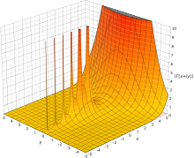
The absolute value of the gamma function on the complex plane.

The behavior of ${\displaystyle \Gamma (z)}$ for an increasing positive variable is simple: it grows quickly — faster than an exponential function. Asymptotically as ${\displaystyle z\to \infty }$, the magnitude of the gamma function is given by Stirling's formula

${\displaystyle \Gamma (z+1)\sim {\sqrt {2\pi z}}\left({\frac {z}{e}}\right)^{z},}$

where the symbol ${\displaystyle \sim }$ means that the ratio of the two sides converges to 1 or asymptotically converges.

Residues

The behavior for non-positive ${\displaystyle z}$ is more intricate. Euler's integral does not converge for ${\displaystyle z\leq 0}$, but the function it defines in the positive complex half-plane has a unique analytic continuation to the negative half-plane. One way to find that analytic continuation is to use Euler's integral for positive arguments and extend the domain to negative numbers by repeated application of the recurrence formula,

${\displaystyle \Gamma (z)={\frac {\Gamma (z+n+1)}{z(z+1)\cdots (z+n)}},}$

choosing ${\displaystyle n}$ such that ${\displaystyle z+n}$ is positive. The product in the denominator is zero when ${\displaystyle z}$ equals any of the integers ${\displaystyle 0,-1,-2,\cdots }$. Thus, the gamma function must be undefined at those points to avoid division by zero; it is a meromorphic function with simple poles at the non-positive integers.
We can rewrite this definition as:

${\displaystyle (z+n)\Gamma (z)={\frac {\Gamma (z+n+1)}{z(z+1)\cdots (z+n-1)}}.}$

At a simple pole c, the residue of f is given by:

${\displaystyle \operatorname {Res} (f,c)=\lim _{z\to c}(z-c)f(z).}$

When ${\displaystyle z=-n,}$

${\displaystyle \Gamma (z+n+1)=\Gamma (1)=1}$

and

${\displaystyle z(z+1)\cdots (z+n-1)=(-1)^{n}n!}$

So the residues of the function at those points are:

${\displaystyle \operatorname {Res} (\Gamma ,-n)={\frac {(-1)^{n}}{n!}}.}$

The gamma function is non-zero everywhere along the real line, although it comes arbitrarily close to zero as z → −∞. There is in fact no complex number ${\displaystyle z}$ for which ${\displaystyle \Gamma (z)=0}$, and hence the reciprocal gamma function ${\displaystyle {\frac {1}{\Gamma (z)}}}$ is an entire function, with zeros at ${\displaystyle z=0,-1,-2,\cdots }$

Minima

The gamma function has a local minimum at ${\displaystyle z_{\mathrm {min} }\approx 1.46163}$ where it attains the value ${\displaystyle \Gamma \left(z_{\mathrm {min} }\right)\approx 0.885603}$. The gamma function must alternate sign between the poles because the product in the forward recurrence contains an odd number of negative factors if the number of poles between ${\displaystyle z}$ and ${\displaystyle z+n}$ is odd, and an even number if the number of poles is even.

Fourier series expansion

The logarithm of the gamma function has the following Fourier series expansion

${\displaystyle \ln \Gamma (z)=\left({\tfrac {1}{2}}-z\right)(\gamma +\ln 2)+(1-z)\ln \pi -{\tfrac {1}{2}}\ln \sin \pi z+{\tfrac {1}{\pi }}\sum _{n=1}^{\infty }{\frac {\sin 2\pi nz\cdot \ln n}{n}}\,,\qquad 0<z<1,}$, where ${\displaystyle \,\gamma \,}$ is the Euler–Mascheroni constant

which was for a long time attributed to Ernst Kummer, who derived it in 1847. However, it was comparatively recently that it was discovered by Iaroslav Blagouchine that this series was first derived by Carl Johan Malmsten in 1842.

Raabe's formula

In 1840 Raabe proved that

${\displaystyle \int _{a}^{a+1}\ln \Gamma (z)\,dz={\tfrac {1}{2}}\ln 2\pi +a\ln a-a,\quad a>0.}$

In particular, if a = 0 then

${\displaystyle \int _{0}^{1}\ln \Gamma (z)\,dz={\tfrac {1}{2}}\ln 2\pi .}$

This formula is used, when one wants to get a convergent version of Stirling's formula. Using the full trapezoidal rule one can show that

${\displaystyle \ln \Gamma (1+z)=z\ln z-z+{\tfrac {1}{2}}\ln 2\pi z+\int _{0}^{\infty }{\frac {2\arctan({\frac {t}{z}})}{e^{2\pi t}-1}}\,dt}$

Pi function

An alternative notation which was originally introduced by Gauss and which was sometimes used is the pi function, which in terms of the gamma function is

${\displaystyle \Pi (z)=\Gamma (z+1)=z\Gamma (z)=\int _{0}^{\infty }e^{-t}t^{z}\,dt,}$

so that Π(n) = n! for every non-negative integer n.
Using the pi function the reflection formula takes on the form

${\displaystyle \Pi (z)\Pi (-z)={\frac {\pi z}{\sin(\pi z)}}={\frac {1}{\operatorname {sinc} (z)}}}$

where sinc is the normalized sinc function, while the multiplication theorem takes on the form

${\displaystyle \Pi \left({\frac {z}{m}}\right)\,\Pi \left({\frac {z-1}{m}}\right)\cdots \Pi \left({\frac {z-m+1}{m}}\right)=(2\pi )^{\frac {m-1}{2}}m^{-z-{\frac {1}{2}}}\Pi (z).}$

We also sometimes find

${\displaystyle \pi (z)={\frac {1}{\Pi (z)}},}$

which is an entire function, defined for every complex number, just like the reciprocal gamma function. That π(z) is entire entails it has no poles, so Π(z), like Γ(z), has no zeros.
The volume of an n-ellipsoid with radii r₁, …, r_n can be expressed as

${\displaystyle V_{n}(r_{1},\dotsc ,r_{n})={\frac {\pi ^{\frac {n}{2}}}{\Pi \left({\frac {n}{2}}\right)}}\prod _{k=1}^{n}r_{k}.}$

Relation to other functions

• In the first integral above, which defines the gamma function, the limits of integration are fixed. The upper and lower incomplete gamma functions are the functions obtained by allowing the lower or upper (respectively) limit of integration to vary.
• The gamma function is related to the beta function by the formula

${\displaystyle \mathrm {B} (x,y)={\frac {\Gamma (x)\;\Gamma (y)}{\Gamma (x+y)}}.}$

• The logarithmic derivative of the gamma function is called the digamma function; higher derivatives are the polygamma functions.
• The analog of the gamma function over a finite field or a finite ring is the Gaussian sums, a type of exponential sum.
• The reciprocal gamma function is an entire function and has been studied as a specific topic.
• The gamma function also shows up in an important relation with the Riemann zeta function, ζ(z).

${\displaystyle \pi ^{-{\frac {z}{2}}}\;\Gamma \left({\frac {z}{2}}\right)\zeta (z)=\pi ^{-{\frac {1-z}{2}}}\;\Gamma \left({\frac {1-z}{2}}\right)\;\zeta (1-z).}$

It also appears in the following formula:

${\displaystyle \zeta (z)\Gamma (z)=\int _{0}^{\infty }{\frac {u^{z}}{e^{u}-1}}\,{\frac {du}{u}},}$

which is valid only for Re(z) > 1.

The logarithm of the gamma function satisfies the following formula due to Lerch:

${\displaystyle \log \Gamma (x)=\zeta _{H}'(0,x)-\zeta '(0),}$

where ζ_H is the Hurwitz zeta function, ζ is the Riemann zeta function and the prime (′) denotes differentiation in the first variable.

• The gamma function is related to the stretched exponential function. For instance, the moments of that function are

${\displaystyle \langle \tau ^{n}\rangle \equiv \int _{0}^{\infty }dt\,t^{n-1}\,e^{-\left({\frac {t}{\tau }}\right)^{\beta }}={\frac {\tau ^{n}}{\beta }}\Gamma \left({n \over \beta }\right).}$

Particular values

 Particular values of the gamma function

Some particular values of the gamma function are:

${\displaystyle {\begin{array}{rcccl}\Gamma \left(-{\tfrac {3}{2}}\right)&=&{\tfrac {4}{3}}{\sqrt {\pi }}&\approx &2.363\,271\,801\,207\\\Gamma \left(-{\tfrac {1}{2}}\right)&=&-2{\sqrt {\pi }}&\approx &-3.544\,907\,701\,811\\\Gamma \left({\tfrac {1}{2}}\right)&=&{\sqrt {\pi }}&\approx &1.772\,453\,850\,906\\\Gamma (1)&=&0!&=&1\\\Gamma \left({\tfrac {3}{2}}\right)&=&{\tfrac {1}{2}}{\sqrt {\pi }}&\approx &0.886\,226\,925\,453\\\Gamma (2)&=&1!&=&1\\\Gamma \left({\tfrac {5}{2}}\right)&=&{\tfrac {3}{4}}{\sqrt {\pi }}&\approx &1.329\,340\,388\,179\\\Gamma (3)&=&2!&=&2\\\Gamma \left({\tfrac {7}{2}}\right)&=&{\tfrac {15}{8}}{\sqrt {\pi }}&\approx &3.323\,350\,970\,448\\\Gamma (4)&=&3!&=&6\end{array}}}$

The complex-valued gamma function is undefined for non-positive integers, but in these cases the value can be defined in the Riemann sphere as ∞. The reciprocal gamma function is well defined and analytic at these values (and in the entire complex plane):

${\displaystyle {\frac {1}{\Gamma (-3)}}={\frac {1}{\Gamma (-2)}}={\frac {1}{\Gamma (-1)}}={\frac {1}{\Gamma (0)}}=0.}$

The log-gamma function

The analytic function log Γ(z)

Because the gamma and factorial functions grow so rapidly for moderately large arguments, many computing environments include a function that returns the natural logarithm of the gamma function (often given the name lgamma or lngamma in programming environments or gammaln in spreadsheets); this grows much more slowly, and for combinatorial calculations allows adding and subtracting logs instead of multiplying and dividing very large values. The digamma function, which is the derivative of this function, is also commonly seen. In the context of technical and physical applications, e.g. with wave propagation, the functional equation

${\displaystyle \ln \Gamma (z)=\ln \Gamma (z+1)-\ln z}$

is often used since it allows one to determine function values in one strip of width 1 in z from the neighbouring strip. In particular, starting with a good approximation for a z with large real part one may go step by step down to the desired z. Following an indication of Carl Friedrich Gauss, Rocktaeschel (1922) proposed for ln(Γ(z)) an approximation for large Re(z):

${\displaystyle \ln \Gamma (z)\approx (z-{\tfrac {1}{2}})\ln z-z+{\tfrac {1}{2}}\ln(2\pi ).}$

This can be used to accurately approximate ln(Γ(z)) for z with a smaller Re(z) via (P.E.Böhmer, 1939)

${\displaystyle \ln \Gamma (z-m)=\ln \Gamma (z)-\sum _{k=1}^{m}\ln(z-k).}$

A more accurate approximation can be obtained by using more terms from the asymptotic expansions of ln(Γ(z)) and Γ(z), which are based on Stirling's approximation.

${\displaystyle \Gamma (z)\sim z^{z-{\frac {1}{2}}}e^{-z}{\sqrt {2\pi }}\left(1+{\frac {1}{12z}}+{\frac {1}{288z^{2}}}-{\frac {139}{51\,840z^{3}}}-{\frac {571}{2\,488\,320z^{4}}}\right)}$

as | z | → ∞ at constant | arg(z) | < π.

In a more "natural" presentation:

${\displaystyle \ln \Gamma (z)\sim z\ln(z)-z-{\tfrac {1}{2}}\ln \left({\frac {z}{2\pi }}\right)+{\frac {1}{12z}}-{\frac {1}{360z^{3}}}+{\frac {1}{1260z^{5}}}}$

as | z | → ∞ at constant | arg(z) | < π.

The coefficients of the terms with k > 1 of z^{−k + 1} in the last expansion are simply

${\displaystyle {\frac {B_{k}}{k(k-1)}}}$

where the B_k are the Bernoulli numbers.

Properties

The Bohr–Mollerup theorem states that among all functions extending the factorial functions to the positive real numbers, only the gamma function is log-convex, that is, its natural logarithm is convex on the positive real axis.
In a certain sense, the ln(Γ) function is the more natural form; it makes some intrinsic attributes of the function clearer. A striking example is the Taylor series of ln(Γ) in 1:

${\displaystyle \ln \Gamma (1+z)=-\gamma z+\sum _{k=2}^{\infty }{\frac {\zeta (k)}{k}}\,(-z)^{k}\qquad \forall \;|z|<1}$

with ζ(k) denoting the Riemann zeta function at k.
So, using the following property:

${\displaystyle \zeta (s)\Gamma (s)=\int _{0}^{\infty }{\frac {t^{s}}{e^{t}-1}}\,{\frac {dt}{t}}}$

we can find an integral representation for the ln(Γ) function:

${\displaystyle \ln \Gamma (1+z)=-\gamma z+\int _{0}^{\infty }{\frac {e^{-zt}-1+zt}{t(e^{t}-1)}}\,dt}$

or, setting z = 1 and calculating γ:

${\displaystyle \ln \Gamma (1+z)=\int _{0}^{\infty }{\frac {e^{-zt}-ze^{-t}-1+z}{t(e^{t}-1)}}\,dt}$

There also exist special formulas for the logarithm of the gamma function for rational z. For instance, if ${\displaystyle k}$ и ${\displaystyle n}$ are integers and ${\displaystyle k<n}$ and ${\displaystyle k\neq n/2}$, then

${\displaystyle \ln \Gamma {\biggl (}\!{\frac {k}{n}}\!{\biggr )}={\frac {(n-2k)\ln 2\pi }{2n}}+{\frac {1}{2}}\left\{\ln \pi -\ln \sin {\frac {\pi k}{n}}\right\}+{\frac {1}{\pi }}\!\sum _{r=1}^{n-1}{\frac {\gamma +\ln {r}}{r}}\cdot \sin {\frac {2\pi rk}{n}}-{\frac {1}{2\pi }}\sin {\frac {2\pi k}{n}}\cdot \!\int _{0}^{\infty }\!\!{\frac {\,e^{-nx}\!\cdot \ln {x}\,}{\,\cosh {x}-\cos {\dfrac {2\pi k}{n}}\,}}\,dx}$

see. This formula is sometimes used for the numerical computation since the integrand decreases very quickly.

Integration over log-gamma

The integral

${\displaystyle \int _{0}^{z}\ln \Gamma (x)\,dx}$

can be expressed in terms of the Barnes G-function (see Barnes G-function for a proof):

${\displaystyle \int _{0}^{z}\ln \Gamma (x)\,dx={\frac {z}{2}}\ln(2\pi )+{\frac {z(1-z)}{2}}+z\ln \Gamma (z)-\ln G(z+1)}$

where Re(z) > −1.
It can also be written in terms of the Hurwitz zeta function:^[14][15]

${\displaystyle \int _{0}^{z}\ln \Gamma (x)\,dx={\frac {z}{2}}\ln(2\pi )+{\frac {z(1-z)}{2}}-\zeta '(-1)+\zeta '(-1,z).}$

Approximations

Comparison gamma (blue line) with the factorial (blue dots) and Stirling's approximation (red line)

Complex values of the gamma function can be computed numerically with arbitrary precision using Stirling's approximation or the Lanczos approximation.
The gamma function can be computed to fixed precision for Re(z) ∈ [1,2] by applying integration by parts to Euler's integral. For any positive number x the gamma function can be written

${\displaystyle {\begin{aligned}\Gamma (z)&=\int _{0}^{x}e^{-t}t^{z}\,{\frac {dt}{t}}+\int _{x}^{\infty }e^{-t}t^{z}\,{\frac {dt}{t}}\\&=x^{z}e^{-x}\sum _{n=0}^{\infty }{\frac {x^{n}}{z(z+1)\cdots (z+n)}}+\int _{x}^{\infty }e^{-t}t^{z}\,{\frac {dt}{t}}.\end{aligned}}}$

When Re(z) ∈ [1,2] and x ≥ 1, the absolute value of the last integral is smaller than (x + 1)e^−x. By choosing a large enough x, this last expression can be made smaller than 2^−N for any desired value N. Thus, the gamma function can be evaluated to N bits of precision with the above series.
The only fast algorithm for calculation of the Euler gamma function for any algebraic argument (including rational) was constructed by E.A. Karatsuba,
For arguments that are integer multiples of 1/24, the gamma function can also be evaluated quickly using arithmetic-geometric mean iterations (see particular values of the gamma function).

Applications

One author describes the gamma function as "Arguably, the most common special function, or the least 'special' of them. The other transcendental functions […] are called 'special' because you could conceivably avoid some of them by staying away from many specialized mathematical topics. On the other hand, the gamma function y = Γ(x) is most difficult to avoid."

Integration problems

The gamma function finds application in such diverse areas as quantum physics, astrophysics and fluid dynamics. The gamma distribution, which is formulated in terms of the gamma function, is used in statistics to model a wide range of processes; for example, the time between occurrences of earthquakes.
The primary reason for the gamma function's usefulness in such contexts is the prevalence of expressions of the type f(t) e^−g(t) which describe processes that decay exponentially in time or space. Integrals of such expressions can occasionally be solved in terms of the gamma function when no elementary solution exists. For example, if f is a power function and g is a linear function, a simple change of variables gives the evaluation

${\displaystyle \int _{0}^{\infty }t^{b}e^{-at}\,dt={\frac {\Gamma (b+1)}{a^{b+1}}}.}$

The fact that the integration is performed along the entire positive real line might signify that the gamma function describes the cumulation of a time-dependent process that continues indefinitely, or the value might be the total of a distribution in an infinite space.
It is of course frequently useful to take limits of integration other than 0 and ∞ to describe the cumulation of a finite process, in which case the ordinary gamma function is no longer a solution; the solution is then called an incomplete gamma function. (The ordinary gamma function, obtained by integrating across the entire positive real line, is sometimes called the complete gamma function for contrast.)
An important category of exponentially decaying functions is that of Gaussian functions

${\displaystyle ae^{-{\frac {(x-b)^{2}}{c^{2}}}}}$

and integrals thereof, such as the error function. There are many interrelations between these functions and the gamma function; notably, √π obtained by evaluating Γ(1/2) is the "same" as that found in the normalizing factor of the error function and the normal distribution.
The integrals we have discussed so far involve transcendental functions, but the gamma function also arises from integrals of purely algebraic functions. In particular, the arc lengths of ellipses and of the lemniscate, which are curves defined by algebraic equations, are given by elliptic integrals that in special cases can be evaluated in terms of the gamma function. The gamma function can also be used to calculate "volume" and "area" of n-dimensional hyperspheres.
Another important special case is that of the beta function

${\displaystyle \mathrm {B} (x,y)=\int _{0}^{1}t^{x-1}(1-t)^{y-1}\,dt={\frac {\Gamma (x)\,\Gamma (y)}{\Gamma (x+y)}}.}$

Calculating products

The gamma function's ability to generalize factorial products immediately leads to applications in many areas of mathematics; in combinatorics, and by extension in areas such as probability theory and the calculation of power series. Many expressions involving products of successive integers can be written as some combination of factorials, the most important example perhaps being that of the binomial coefficient

${\displaystyle {\binom {n}{k}}={\frac {n!}{k!(n-k)!}}.}$

The example of binomial coefficients motivates why the properties of the gamma function when extended to negative numbers are natural. A binomial coefficient gives the number of ways to choose k elements from a set of n elements; if k > n, there are of course no ways. If k > n, (n − k)! is the factorial of a negative integer and hence infinite if we use the gamma function definition of factorials — dividing by infinity gives the expected value of 0.
We can replace the factorial by a gamma function to extend any such formula to the complex numbers. Generally, this works for any product wherein each factor is a rational function of the index variable, by factoring the rational function into linear expressions. If P and Q are monic polynomials of degree m and n with respective roots p₁, …, p_m and q₁, …, q_n, we have

${\displaystyle \prod _{i=a}^{b}{\frac {P(i)}{Q(i)}}=\left(\prod _{j=1}^{m}{\frac {\Gamma (b-p_{j}+1)}{\Gamma (a-p_{j})}}\right)\left(\prod _{k=1}^{n}{\frac {\Gamma (a-q_{k})}{\Gamma (b-q_{k}+1)}}\right).}$

If we have a way to calculate the gamma function numerically, it is a breeze to calculate numerical values of such products. The number of gamma functions in the right-hand side depends only on the degree of the polynomials, so it does not matter whether b − a equals 5 or 10⁵. By taking the appropriate limits, the equation can also be made to hold even when the left-hand product contains zeros or poles.
By taking limits, certain rational products with infinitely many factors can be evaluated in terms of the gamma function as well. Due to the Weierstrass factorization theorem, analytic functions can be written as infinite products, and these can sometimes be represented as finite products or quotients of the gamma function. We have already seen one striking example: the reflection formula essentially represents the sine function as the product of two gamma functions. Starting from this formula, the exponential function as well as all the trigonometric and hyperbolic functions can be expressed in terms of the gamma function.
More functions yet, including the hypergeometric function and special cases thereof, can be represented by means of complex contour integrals of products and quotients of the gamma function, called Mellin-Barnes integrals.

Analytic number theory

An elegant and deep application of the gamma function is in the study of the Riemann zeta function. A fundamental property of the Riemann zeta function is its functional equation:

${\displaystyle \Gamma \left({\frac {s}{2}}\right)\zeta (s)\pi ^{-{\frac {s}{2}}}=\Gamma \left({\frac {1-s}{2}}\right)\zeta (1-s)\pi ^{-{\frac {1-s}{2}}}.}$

Among other things, this provides an explicit form for the analytic continuation of the zeta function to a meromorphic function in the complex plane and leads to an immediate proof that the zeta function has infinitely many so-called "trivial" zeros on the real line. Borwein et al. call this formula "one of the most beautiful findings in mathematics". Another champion for that title might be

${\displaystyle \zeta (s)\;\Gamma (s)=\int _{0}^{\infty }{\frac {t^{s}}{e^{t}-1}}\,{\frac {dt}{t}}.}$

Both formulas were derived by Bernhard Riemann in his seminal 1859 paper "Über die Anzahl der Primzahlen unter einer gegebenen Größe" ("On the Number of Prime Numbers less than a Given Quantity"), one of the milestones in the development of analytic number theory — the branch of mathematics that studies prime numbers using the tools of mathematical analysis. Factorial numbers, considered as discrete objects, are an important concept in classical number theory because they contain many prime factors, but Riemann found a use for their continuous extension that arguably turned out to be even more important.

a bright cloud under the star

The gamma function has caught the interest of some of the most prominent mathematicians of all time. Its history, notably documented by Philip J. Davis in an article that won him the 1963 Chauvenet Prize, reflects many of the major developments within mathematics since the 18th century. In the words of Davis, "each generation has found something of interest to say about the gamma function. Perhaps the next generation will also."

18th century: Euler and Stirling

Daniel Bernoulli's letter to Christian Goldbach, October 6, 1729

The problem of extending the factorial to non-integer arguments was apparently first considered by Daniel Bernoulli and Christian Goldbach in the 1720s, and was solved at the end of the same decade by Leonhard Euler. Euler gave two different definitions: the first was not his integral but an infinite product,

${\displaystyle n!=\prod _{k=1}^{\infty }{\frac {\left(1+{\frac {1}{k}}\right)^{n}}{1+{\frac {n}{k}}}}\,,}$

of which he informed Goldbach in a letter dated October 13, 1729. He wrote to Goldbach again on January 8, 1730, to announce his discovery of the integral representation

${\displaystyle n!=\int _{0}^{1}(-\ln s)^{n}\,ds\,,}$

which is valid for n > 0. By the change of variables t = −ln s, this becomes the familiar Euler integral. Euler published his results in the paper "De progressionibus transcendentibus seu quarum termini generales algebraice dari nequeunt" ("On transcendental progressions, that is, those whose general terms cannot be given algebraically"), submitted to the St. Petersburg Academy on November 28, 1729. Euler further discovered some of the gamma function's important functional properties, including the reflection formula.
James Stirling, a contemporary of Euler, also attempted to find a continuous expression for the factorial and came up with what is now known as Stirling's formula. Although Stirling's formula gives a good estimate of n!, also for non-integers, it does not provide the exact value. Extensions of his formula that correct the error were given by Stirling himself and by Jacques Philippe Marie Binet.

19th century: Gauss, Weierstrass and Legendre

The first page of Euler's paper

Carl Friedrich Gauss rewrote Euler's product as

${\displaystyle \Gamma (z)=\lim _{m\to \infty }{\frac {m^{z}m!}{z(z+1)(z+2)\cdots (z+m)}}}$

and used this formula to discover new properties of the gamma function. Although Euler was a pioneer in the theory of complex variables, he does not appear to have considered the factorial of a complex number, as instead Gauss first did. Gauss also proved the multiplication theorem of the gamma function and investigated the connection between the gamma function and elliptic integrals.
Karl Weierstrass further established the role of the gamma function in complex analysis, starting from yet another product representation,

${\displaystyle \Gamma (z)={\frac {e^{-\gamma z}}{z}}\prod _{k=1}^{\infty }\left(1+{\frac {z}{k}}\right)^{-1}e^{\frac {z}{k}},}$

where γ is the Euler–Mascheroni constant. Weierstrass originally wrote his product as one for 1/Γ, in which case it is taken over the function's zeros rather than its poles. Inspired by this result, he proved what is known as the Weierstrass factorization theorem—that any entire function can be written as a product over its zeros in the complex plane; a generalization of the fundamental theorem of algebra.
The name gamma function and the symbol Γ were introduced by Adrien-Marie Legendre around 1811; Legendre also rewrote Euler's integral definition in its modern form. Although the symbol is an upper-case Greek gamma, there is no accepted standard for whether the function name should be written "gamma function" or "Gamma function" (some authors simply write "Γ-function"). The alternative "pi function" notation Π(z) = z! due to Gauss is sometimes encountered in older literature, but Legendre's notation is dominant in modern works.
It is justified to ask why we distinguish between the "ordinary factorial" and the gamma function by using distinct symbols, and particularly why the gamma function should be normalized to Γ(n + 1) = n! instead of simply using "Γ(n) = n!". Consider that the notation for exponents, xⁿ, has been generalized from integers to complex numbers x^z without any change. Legendre's motivation for the normalization does not appear to be known, and has been criticized as cumbersome by some (the 20th-century mathematician Cornelius Lanczos, for example, called it "void of any rationality" and would instead use z!). Legendre's normalization does simplify a few formulae, but complicates most others. From a modern point of view, the Legendre normalization of the Gamma function is the integral of the additive character e^−x against the multiplicative character x^z with respect to the Haar measure ${\displaystyle {\tfrac {dx}{x}}}$ on the Lie group R⁺. Thus this normalization makes it clearer that the gamma function is a continuous analogue of a Gauss sum.

19th–20th centuries: characterizing the gamma function

It is somewhat problematic that a large number of definitions have been given for the gamma function. Although they describe the same function, it is not entirely straightforward to prove the equivalence. Stirling never proved that his extended formula corresponds exactly to Euler's gamma function; a proof was first given by Charles Hermite in 1900. Instead of finding a specialized proof for each formula, it would be desirable to have a general method of identifying the gamma function.
One way to prove would be to find a differential equation that characterizes the gamma function. Most special functions in applied mathematics arise as solutions to differential equations, whose solutions are unique. However, the gamma function does not appear to satisfy any simple differential equation. Otto Hölder proved in 1887 that the gamma function at least does not satisfy any algebraic differential equation by showing that a solution to such an equation could not satisfy the gamma function's recurrence formula, making it a transcendentally transcendental function. This result is known as Hölder's theorem.
A definite and generally applicable characterization of the gamma function was not given until 1922. Harald Bohr and Johannes Mollerup then proved what is known as the Bohr–Mollerup theorem: that the gamma function is the unique solution to the factorial recurrence relation that is positive and logarithmically convex for positive z and whose value at 1 is 1 (a function is logarithmically convex if its logarithm is convex).
The Bohr–Mollerup theorem is useful because it is relatively easy to prove logarithmic convexity for any of the different formulas used to define the gamma function. Taking things further, instead of defining the gamma function by any particular formula, we can choose the conditions of the Bohr–Mollerup theorem as the definition, and then pick any formula we like that satisfies the conditions as a starting point for studying the gamma function. This approach was used by the Bourbaki group.

Borwein & Corless rewiew three centuries of work on the gamma function.

Reference tables and software

Although the gamma function can be calculated virtually as easily as any mathematically simpler function with a modern computer—even with a programmable pocket calculator—this was of course not always the case. Until the mid-20th century, mathematicians relied on hand-made tables; in the case of the gamma function, notably a table computed by Gauss in 1813 and one computed by Legendre in 1825.

A hand-drawn graph of the absolute value of the complex gamma function, from Tables of Higher Functions by Jahnke and Emde.

Tables of complex values of the gamma function, as well as hand-drawn graphs, were given in Tables of Higher Functions by Jahnke and Emde, first published in Germany in 1909. According to Michael Berry, "the publication in J&E of a three-dimensional graph showing the poles of the gamma function in the complex plane acquired an almost iconic status."
There was in fact little practical need for anything but real values of the gamma function until the 1930s, when applications for the complex gamma function were discovered in theoretical physics. As electronic computers became available for the production of tables in the 1950s, several extensive tables for the complex gamma function were published to meet the demand, including a table accurate to 12 decimal places from the U.S. National Bureau of Standards.
Abramowitz and Stegun became the standard reference for this and many other special functions after its publication in 1964.
Double-precision floating-point implementations of the gamma function and its logarithm are now available in most scientific computing software and special functions libraries, for example TK Solver, Matlab, GNU Octave, and the GNU Scientific Library. The gamma function was also added to the C standard library (math.h). Arbitrary-precision implementations are available in most computer algebra systems, such as Mathematica and Maple. PARI/GP, MPFR and MPFUN contain free arbitrary-precision implementations. A little-known feature of the calculator app included with the Android operating system is that it will accept fractional values as input to the factorial function and return the equivalent gamma function value. The same is true for Windows Calculator (in scientific mode).   



                                                                  X  .  III 
                                                        Information theory  

Information theory studies the quantification, storage, and communication of information. It was originally proposed by Claude E. Shannon in 1948 to find fundamental limits on signal processing and communication operations such as data compression, in a landmark paper entitled "A Mathematical Theory of Communication". Now this theory has found applications in many other areas, including statistical inference, natural language processing, cryptography, neurobiology,^[1] the evolution^[2] and function^[3] of molecular codes, model selection in ecology,^[4] thermal physics,^[5] quantum computing, linguistics, plagiarism detection,^[6] pattern recognition, and anomaly detection.^[7]
A key measure in information theory is "entropy". Entropy quantifies the amount of uncertainty involved in the value of a random variable or the outcome of a random process. For example, identifying the outcome of a fair coin flip (with two equally likely outcomes) provides less information (lower entropy) than specifying the outcome from a roll of a die (with six equally likely outcomes). Some other important measures in information theory are mutual information, channel capacity, error exponents, and relative entropy.
Applications of fundamental topics of information theory include lossless data compression (e.g. ZIP files), lossy data compression (e.g. MP3s and JPEGs), and channel coding (e.g. for digital subscriber line (DSL)).
The field is at the intersection of mathematics, statistics, computer science, physics, neurobiology, and electrical engineering. Its impact has been crucial to the success of the Voyager missions to deep space, the invention of the compact disc, the feasibility of mobile phones, the development of the Internet, the study of linguistics and of human perception, the understanding of black holes, and numerous other fields. Important sub-fields of information theory include source coding, channel coding, algorithmic complexity theory, algorithmic information theory, information-theoretic security, and measures of information. 

Overview

Information theory studies the transmission, processing, utilization, and extraction of information. Abstractly, information can be thought of as the resolution of uncertainty. In the case of communication of information over a noisy channel, this abstract concept was made concrete in 1948 by Claude Shannon in his paper "A Mathematical Theory of Communication", in which "information" is thought of as a set of possible messages, where the goal is to send these messages over a noisy channel, and then to have the receiver reconstruct the message with low probability of error, in spite of the channel noise. Shannon's main result, the noisy-channel coding theorem showed that, in the limit of many channel uses, the rate of information that is asymptotically achievable is equal to the channel capacity, a quantity dependent merely on the statistics of the channel over which the messages are sent.
Information theory is closely associated with a collection of pure and applied disciplines that have been investigated and reduced to engineering practice under a variety of rubrics throughout the world over the past half century or more: adaptive systems, anticipatory systems, artificial intelligence, complex systems, complexity science, cybernetics, informatics, machine learning, along with systems sciences of many descriptions. Information theory is a broad and deep mathematical theory, with equally broad and deep applications, amongst which is the vital field of coding theory.
Coding theory is concerned with finding explicit methods, called codes, for increasing the efficiency and reducing the error rate of data communication over noisy channels to near the channel capacity. These codes can be roughly subdivided into data compression (source coding) and error-correction (channel coding) techniques. In the latter case, it took many years to find the methods Shannon's work proved were possible. A third class of information theory codes are cryptographic algorithms (both codes and ciphers). Concepts, methods and results from coding theory and information theory are widely used in cryptography and cryptanalysis. See the article ban (unit) for a historical application.
Information theory is also used in information retrieval, intelligence gathering, gambling, statistics, and even in musical composition.

The landmark event that established the discipline of information theory and brought it to immediate worldwide attention was the publication of Claude E. Shannon's classic paper "A Mathematical Theory of Communication" in the Bell System Technical Journal in July and October 1948.
Prior to this paper, limited information-theoretic ideas had been developed at Bell Labs, all implicitly assuming events of equal probability. Harry Nyquist's 1924 paper, Certain Factors Affecting Telegraph Speed, contains a theoretical section quantifying "intelligence" and the "line speed" at which it can be transmitted by a communication system, giving the relation W = K log m (recalling Boltzmann's constant), where W is the speed of transmission of intelligence, m is the number of different voltage levels to choose from at each time step, and K is a constant. Ralph Hartley's 1928 paper, Transmission of Information, uses the word information as a measurable quantity, reflecting the receiver's ability to distinguish one sequence of symbols from any other, thus quantifying information as H = log Sⁿ = n log S, where S was the number of possible symbols, and n the number of symbols in a transmission. The unit of information was therefore the decimal digit, much later renamed the hartley in his honour as a unit or scale or measure of information. Alan Turing in 1940 used similar ideas as part of the statistical analysis of the breaking of the German second world war Enigma ciphers.
Much of the mathematics behind information theory with events of different probabilities were developed for the field of thermodynamics by Ludwig Boltzmann and J. Willard Gibbs. Connections between information-theoretic entropy and thermodynamic entropy, including the important contributions by Rolf Landauer in the 1960s, are explored in Entropy in thermodynamics and information theory.
In Shannon's revolutionary and groundbreaking paper, the work for which had been substantially completed at Bell Labs by the end of 1944, Shannon for the first time introduced the qualitative and quantitative model of communication as a statistical process underlying information theory, opening with the assertion that

"The fundamental problem of communication is that of reproducing at one point, either exactly or approximately, a message selected at another point."

With it came the ideas of

• the information entropy and redundancy of a source, and its relevance through the source coding theorem;
• the mutual information, and the channel capacity of a noisy channel, including the promise of perfect loss-free communication given by the noisy-channel coding theorem;
• the practical result of the Shannon–Hartley law for the channel capacity of a Gaussian channel; as well as
• the bit—a new way of seeing the most fundamental unit of information.

Quantities of information

Quantities of information

Information theory is based on probability theory and statistics. Information theory often concerns itself with measures of information of the distributions associated with random variables. Important quantities of information are entropy, a measure of information in a single random variable, and mutual information, a measure of information in common between two random variables. The former quantity is a property of the probability distribution of a random variable and gives a limit on the rate at which data generated by independent samples with the given distribution can be reliably compressed. The latter is a property of the joint distribution of two random variables, and is the maximum rate of reliable communication across a noisy channel in the limit of long block lengths, when the channel statistics are determined by the joint distribution.
The choice of logarithmic base in the following formulae determines the unit of information entropy that is used. A common unit of information is the bit, based on the binary logarithm. Other units include the nat, which is based on the natural logarithm, and the hartley, which is based on the common logarithm.
In what follows, an expression of the form p log p is considered by convention to be equal to zero whenever p = 0. This is justified because ${\displaystyle \lim _{p\rightarrow 0+}p\log p=0}$ for any logarithmic base.

Entropy of an information source

Based on the probability mass function of each source symbol to be communicated, the Shannon entropy H, in units of bits (per symbol), is given by

${\displaystyle H=-\sum _{i}p_{i}\log _{2}(p_{i})}$

where p_i is the probability of occurrence of the i-th possible value of the source symbol. This equation gives the entropy in the units of "bits" (per symbol) because it uses a logarithm of base 2, and this base-2 measure of entropy has sometimes been called the "shannon" in his honor. Entropy is also commonly computed using the natural logarithm (base e, where e is Euler's number), which produces a measurement of entropy in "nats" per symbol and sometimes simplifies the analysis by avoiding the need to include extra constants in the formulas. Other bases are also possible, but less commonly used. For example, a logarithm of base 2⁸ = 256 will produce a measurement in bytes per symbol, and a logarithm of base 10 will produce a measurement in decimal digits (or hartleys) per symbol.
Intuitively, the entropy H_X of a discrete random variable X is a measure of the amount of uncertainty associated with the value of X when only its distribution is known.
The entropy of a source that emits a sequence of N symbols that are independent and identically distributed (iid) is N·H bits (per message of N symbols). If the source data symbols are identically distributed but not independent, the entropy of a message of length N will be less than N·H.

The entropy of a Bernoulli trial as a function of success probability, often called the binary entropy function, H_b(p). The entropy is maximized at 1 bit per trial when the two possible outcomes are equally probable, as in an unbiased coin toss.

If one transmits 1000 bits (0s and 1s), and the value of each of these bits is known to the receiver (has a specific value with certainty) ahead of transmission, it is clear that no information is transmitted. If, however, each bit is independently equally likely to be 0 or 1, 1000 shannons of information (more often called bits) have been transmitted. Between these two extremes, information can be quantified as follows. If 𝕏 is the set of all messages {x₁, …, x_n} that X could be, and p(x) is the probability of some ${\displaystyle x\in \mathbb {X} }$, then the entropy, H, of X is defined:

${\displaystyle H(X)=\mathbb {E} _{X}[I(x)]=-\sum _{x\in \mathbb {X} }p(x)\log p(x).}$

(Here, I(x) is the self-information, which is the entropy contribution of an individual message, and 𝔼_X is the expected value.) A property of entropy is that it is maximized when all the messages in the message space are equiprobable p(x) = 1/n; i.e., most unpredictable, in which case H(X) = log n.
The special case of information entropy for a random variable with two outcomes is the binary entropy function, usually taken to the logarithmic base 2, thus having the shannon (Sh) as unit:

${\displaystyle H_{\mathrm {b} }(p)=-p\log _{2}p-(1-p)\log _{2}(1-p).}$

Joint entropy

The joint entropy of two discrete random variables X and Y is merely the entropy of their pairing: (X, Y). This implies that if X and Y are independent, then their joint entropy is the sum of their individual entropies.
For example, if (X, Y) represents the position of a chess piece — X the row and Y the column, then the joint entropy of the row of the piece and the column of the piece will be the entropy of the position of the piece.

${\displaystyle H(X,Y)=\mathbb {E} _{X,Y}[-\log p(x,y)]=-\sum _{x,y}p(x,y)\log p(x,y)\,}$

Despite similar notation, joint entropy should not be confused with cross entropy.

Conditional entropy (equivocation)

The conditional entropy or conditional uncertainty of X given random variable Y (also called the equivocation of X about Y) is the average conditional entropy over Y:

${\displaystyle H(X|Y)=\mathbb {E} _{Y}[H(X|y)]=-\sum _{y\in Y}p(y)\sum _{x\in X}p(x|y)\log p(x|y)=-\sum _{x,y}p(x,y)\log {\frac {p(x|y)}{p(x)}}.}$

Because entropy can be conditioned on a random variable or on that random variable being a certain value, care should be taken not to confuse these two definitions of conditional entropy, the former of which is in more common use. A basic property of this form of conditional entropy is that:

${\displaystyle H(X|Y)=H(X,Y)-H(Y).\,}$

Mutual information (transinformation)

Mutual information measures the amount of information that can be obtained about one random variable by observing another. It is important in communication where it can be used to maximize the amount of information shared between sent and received signals. The mutual information of X relative to Y is given by:

${\displaystyle I(X;Y)=\mathbb {E} _{X,Y}[SI(x,y)]=\sum _{x,y}p(x,y)\log {\frac {p(x,y)}{p(x)\,p(y)}}}$

where SI (Specific mutual Information) is the pointwise mutual information.
A basic property of the mutual information is that

${\displaystyle I(X;Y)=H(X)-H(X|Y).\,}$

That is, knowing Y, we can save an average of I(X; Y) bits in encoding X compared to not knowing Y.
Mutual information is symmetric:

${\displaystyle I(X;Y)=I(Y;X)=H(X)+H(Y)-H(X,Y).\,}$

Mutual information can be expressed as the average Kullback–Leibler divergence (information gain) between the posterior probability distribution of X given the value of Y and the prior distribution on X:

${\displaystyle I(X;Y)=\mathbb {E} _{p(y)}[D_{\mathrm {KL} }(p(X|Y=y)\|p(X))].}$

In other words, this is a measure of how much, on the average, the probability distribution on X will change if we are given the value of Y. This is often recalculated as the divergence from the product of the marginal distributions to the actual joint distribution:

${\displaystyle I(X;Y)=D_{\mathrm {KL} }(p(X,Y)\|p(X)p(Y)).}$

Mutual information is closely related to the log-likelihood ratio test in the context of contingency tables and the multinomial distribution and to Pearson's χ² test: mutual information can be considered a statistic for assessing independence between a pair of variables, and has a well-specified asymptotic distribution.

Kullback–Leibler divergence (information gain)

The Kullback–Leibler divergence (or information divergence, information gain, or relative entropy) is a way of comparing two distributions: a "true" probability distribution p(X), and an arbitrary probability distribution q(X). If we compress data in a manner that assumes q(X) is the distribution underlying some data, when, in reality, p(X) is the correct distribution, the Kullback–Leibler divergence is the number of average additional bits per datum necessary for compression. It is thus defined

${\displaystyle D_{\mathrm {KL} }(p(X)\|q(X))=\sum _{x\in X}-p(x)\log {q(x)}\,-\,\sum _{x\in X}-p(x)\log {p(x)}=\sum _{x\in X}p(x)\log {\frac {p(x)}{q(x)}}.}$

Although it is sometimes used as a 'distance metric', KL divergence is not a true metric since it is not symmetric and does not satisfy the triangle inequality (making it a semi-quasimetric).
Another interpretation of the KL divergence is the "unnecessary surprise" introduced by a prior from the truth: suppose a number X is about to be drawn randomly from a discrete set with probability distribution p(x). If Alice knows the true distribution p(x), while Bob believes (has a prior) that the distribution is q(x), then Bob will be more surprised than Alice, on average, upon seeing the value of X. The KL divergence is the (objective) expected value of Bob's (subjective) surprisal minus Alice's surprisal, measured in bits if the log is in base 2. In this way, the extent to which Bob's prior is "wrong" can be quantified in terms of how "unnecessarily surprised" it is expected to make him.

Other quantities

Other important information theoretic quantities include Rényi entropy (a generalization of entropy), differential entropy (a generalization of quantities of information to continuous distributions), and the conditional mutual information.

Coding theory

 Coding theory

A picture showing scratches on the readable surface of a CD-R. Music and data CDs are coded using error correcting codes and thus can still be read even if they have minor scratches using error detection and correction.

Coding theory is one of the most important and direct applications of information theory. It can be subdivided into source coding theory and channel coding theory. Using a statistical description for data, information theory quantifies the number of bits needed to describe the data, which is the information entropy of the source.

• Data compression (source coding): There are two formulations for the compression problem:
• lossless data compression: the data must be reconstructed exactly;
• lossy data compression: allocates bits needed to reconstruct the data, within a specified fidelity level measured by a distortion function. This subset of information theory is called rate–distortion theory.

• Error-correcting codes (channel coding): While data compression removes as much redundancy as possible, an error correcting code adds just the right kind of redundancy (i.e., error correction) needed to transmit the data efficiently and faithfully across a noisy channel.

This division of coding theory into compression and transmission is justified by the information transmission theorems, or source–channel separation theorems that justify the use of bits as the universal currency for information in many contexts. However, these theorems only hold in the situation where one transmitting user wishes to communicate to one receiving user. In scenarios with more than one transmitter (the multiple-access channel), more than one receiver (the broadcast channel) or intermediary "helpers" (the relay channel), or more general networks, compression followed by transmission may no longer be optimal. Network information theory refers to these multi-agent communication models.

Source theory

Any process that generates successive messages can be considered a source of information. A memoryless source is one in which each message is an independent identically distributed random variable, whereas the properties of ergodicity and stationarity impose less restrictive constraints. All such sources are stochastic. These terms are well studied in their own right outside information theory.

Rate

Information rate is the average entropy per symbol. For memoryless sources, this is merely the entropy of each symbol, while, in the case of a stationary stochastic process, it is

${\displaystyle r=\lim _{n\to \infty }H(X_{n}|X_{n-1},X_{n-2},X_{n-3},\ldots );}$

that is, the conditional entropy of a symbol given all the previous symbols generated. For the more general case of a process that is not necessarily stationary, the average rate is

${\displaystyle r=\lim _{n\to \infty }{\frac {1}{n}}H(X_{1},X_{2},\dots X_{n});}$

that is, the limit of the joint entropy per symbol. For stationary sources, these two expressions give the same result.
It is common in information theory to speak of the "rate" or "entropy" of a language. This is appropriate, for example, when the source of information is English prose. The rate of a source of information is related to its redundancy and how well it can be compressed, the subject of source coding.

Channel capacity

 Channel capacity

Communications over a channel—such as an ethernet cable—is the primary motivation of information theory. As anyone who's ever used a telephone (mobile or landline) knows, however, such channels often fail to produce exact reconstruction of a signal; noise, periods of silence, and other forms of signal corruption often degrade quality.
Consider the communications process over a discrete channel. A simple model of the process is shown below:

Here X represents the space of messages transmitted, and Y the space of messages received during a unit time over our channel. Let p(y|x) be the conditional probability distribution function of Y given X. We will consider p(y|x) to be an inherent fixed property of our communications channel (representing the nature of the noise of our channel). Then the joint distribution of X and Y is completely determined by our channel and by our choice of f(x), the marginal distribution of messages we choose to send over the channel. Under these constraints, we would like to maximize the rate of information, or the signal, we can communicate over the channel. The appropriate measure for this is the mutual information, and this maximum mutual information is called the channel capacity and is given by:

${\displaystyle C=\max _{f}I(X;Y).\!}$

This capacity has the following property related to communicating at information rate R (where R is usually bits per symbol). For any information rate R < C and coding error ε > 0, for large enough N, there exists a code of length N and rate ≥ R and a decoding algorithm, such that the maximal probability of block error is ≤ ε; that is, it is always possible to transmit with arbitrarily small block error. In addition, for any rate R > C, it is impossible to transmit with arbitrarily small block error.
Channel coding is concerned with finding such nearly optimal codes that can be used to transmit data over a noisy channel with a small coding error at a rate near the channel capacity.

Capacity of particular channel models

• A continuous-time analog communications channel subject to Gaussian noise — see Shannon–Hartley theorem.
• A binary symmetric channel (BSC) with crossover probability p is a binary input, binary output channel that flips the input bit with probability p. The BSC has a capacity of 1 − H_b(p) bits per channel use, where H_b is the binary entropy function to the base-2 logarithm:

• A binary erasure channel (BEC) with erasure probability p is a binary input, ternary output channel. The possible channel outputs are 0, 1, and a third symbol 'e' called an erasure. The erasure represents complete loss of information about an input bit. The capacity of the BEC is 1 − p bits per channel use.

Applications to other fields

Intelligence uses and secrecy applications

Information theoretic concepts apply to cryptography and cryptanalysis. Turing's information unit, the ban, was used in the Ultra project, breaking the German Enigma machine code and hastening the end of World War II in Europe. Shannon himself defined an important concept now called the unicity distance. Based on the redundancy of the plaintext, it attempts to give a minimum amount of ciphertext necessary to ensure unique decipherability.
Information theory leads us to believe it is much more difficult to keep secrets than it might first appear. A brute force attack can break systems based on asymmetric key algorithms or on most commonly used methods of symmetric key algorithms (sometimes called secret key algorithms), such as block ciphers. The security of all such methods currently comes from the assumption that no known attack can break them in a practical amount of time.
Information theoretic security refers to methods such as the one-time pad that are not vulnerable to such brute force attacks. In such cases, the positive conditional mutual information between the plaintext and ciphertext (conditioned on the key) can ensure proper transmission, while the unconditional mutual information between the plaintext and ciphertext remains zero, resulting in absolutely secure communications. In other words, an eavesdropper would not be able to improve his or her guess of the plaintext by gaining knowledge of the ciphertext but not of the key. However, as in any other cryptographic system, care must be used to correctly apply even information-theoretically secure methods; the Venona project was able to crack the one-time pads of the Soviet Union due to their improper reuse of key material.

Pseudorandom number generation

Pseudorandom number generators are widely available in computer language libraries and application programs. They are, almost universally, unsuited to cryptographic use as they do not evade the deterministic nature of modern computer equipment and software. A class of improved random number generators is termed cryptographically secure pseudorandom number generators, but even they require random seeds external to the software to work as intended. These can be obtained via extractors, if done carefully. The measure of sufficient randomness in extractors is min-entropy, a value related to Shannon entropy through Rényi entropy; Rényi entropy is also used in evaluating randomness in cryptographic systems. Although related, the distinctions among these measures mean that a random variable with high Shannon entropy is not necessarily satisfactory for use in an extractor and so for cryptography uses.

Seismic exploration

One early commercial application of information theory was in the field of seismic oil exploration. Work in this field made it possible to strip off and separate the unwanted noise from the desired seismic signal. Information theory and digital signal processing offer a major improvement of resolution and image clarity over previous analog methods.

Semiotics

Concepts from information theory such as redundancy and code control have been used by semioticians such as Umberto Eco and Ferruccio Rossi-Landi to explain ideology as a form of message transmission whereby a dominant social class emits its message by using signs that exhibit a high degree of redundancy such that only one message is decoded among a selection of competing ones.

Miscellaneous applications

Information theory also has applications in The essence of atoms, gambling and investing, black holes, and bioinformatics.  


   
    

                                                             The Intelligence Cycle       




                                                                   X  .  IIII  

                                              Field-Programmable Gate Array   


Field-Programmable Gate Array (FPGA) is a digital IC that is often used to implement digital circuits. FPGAs are electronics and semiconductor components consisting of programmable logic components and programmed (interconnected) connections. The programmed gate components include the usual logical gate types (AND, OR, NOT) as well as more complex types of mathematical and combinatorial functions, such as decoders, adders, subtractors, multipliers, etc. The component blocks inside the FPGA can also contain memory elements (registers) ranging from flip-flops to RAM (Random Access Memory). FPGA is particularly suitable for computational processing of numerical integration algorithms. The advantages of FPGA implementation are used to improve design efficiency by reducing the use of software programming. FPGA has a small error correction and is a technology-independent technology to be implemented in various algorithms. FPGA application performance is faster than microcontroller application, because FPGA only synthesizes hardware, while microcontroller executes software instruction used to control hardware, so that the delayed time is only time-consuming delay of propagation (Propagation delay) only. FPGA modeling requires information related to the level of abstraction differences and the type of model used. An FPGA designer must be able to take several modeling stages to ensure the results of the design model through the simulation model provided by the respective FPGA vendor.  

 

  

 FPGA type Altera StratixIVGXThe programmable in the FPGA is similar to the switchboard interconnect in a breadboard that can be changed by the designer according to the needs of the user. In FPGA, these interconnections can be reprogrammed by users or designers in the lab or field. Therefore the range of logic gate (Gate Array) is called field-programmable. A programmable type of programmable gate encompasses all basic gateways to suit any need. 

 

Reasons for using FPGA
Has the ability to handle such a heavy computing load
Eliminate the intensive tasks of Digital Signal Processing
Customize the architecture to fit the ideal algorithm.
Reduce system costs.
Cost efficiency.  

Field-programmable gate array

         

"FPGA" redirects here. It is not to be confused with Flip-chip pin grid array.

A Stratix IV FPGA from Altera

A field-programmable gate array (FPGA) is an integrated circuit designed to be configured by a customer or a designer after manufacturing – hence "field-programmable". The FPGA configuration is generally specified using a hardware description language (HDL), similar to that used for an application-specific integrated circuit (ASIC). (Circuit diagrams were previously used to specify the configuration, as they were for ASICs, but this is increasingly rare.)

A Spartan FPGA from Xilinx

FPGAs contain an array of programmable logic blocks, and a hierarchy of reconfigurable interconnects that allow the blocks to be "wired together", like many logic gates that can be inter-wired in different configurations. Logic blocks can be configured to perform complex combinational functions, or merely simple logic gates like AND and XOR. In most FPGAs, logic blocks also include memory elements, which may be simple flip-flops or more complete blocks of memory.

 

Technical design

Contemporary field-programmable gate arrays (FPGAs) have large resources of logic gates and RAM blocks to implement complex digital computations. As FPGA designs employ very fast I/Os and bidirectional data buses, it becomes a challenge to verify correct timing of valid data within setup time and hold time. Floor planning enables resources allocation within FPGAs to meet these time constraints. FPGAs can be used to implement any logical function that an ASIC could perform. The ability to update the functionality after shipping, partial re-configuration of a portion of the designand the low non-recurring engineering costs relative to an ASIC design (notwithstanding the generally higher unit cost), offer advantages for many applications.
Some FPGAs have analog features in addition to digital functions. The most common analog feature is programmable slew rate on each output pin, allowing the engineer to set low rates on lightly loaded pins that would otherwise ring or couple unacceptably, and to set higher rates on heavily loaded pins on high-speed channels that would otherwise run too slowly. Also common are quartz-crystal oscillators, on-chip resistance-capacitance oscillators, and phase-locked loops with embedded voltage-controlled oscillators used for clock generation and management and for high-speed serializer-deserializer (SERDES) transmit clocks and receiver clock recovery. Fairly common are differential comparators on input pins designed to be connected to differential signaling channels. A few "mixed signal FPGAs" have integrated peripheral analog-to-digital converters (ADCs) and digital-to-analog converters (DACs) with analog signal conditioning blocks allowing them to operate as a system-on-a-chip. Such devices blur the line between an FPGA, which carries digital ones and zeros on its internal programmable interconnect fabric, and field-programmable analog array (FPAA), which carries analog values on its internal programmable interconnect fabric.

History

The FPGA industry sprouted from programmable read-only memory (PROM) and programmable logic devices (PLDs). PROMs and PLDs both had the option of being programmed in batches in a factory or in the field (field-programmable). However, programmable logic was hard-wired between logic gates.
In the late 1980s, the Naval Surface Warfare Center funded an experiment proposed by Steve Casselman to develop a computer that would implement 600,000 reprogrammable gates. Casselman was successful and a patent related to the system was issued in 1992.
Some of the industry's foundational concepts and technologies for programmable logic arrays, gates, and logic blocks are founded in patents awarded to David W. Page and LuVerne R. Peterson in 1985
Altera was founded in 1983 and delivered the industry's first reprogrammable logic device in 1984 – the EP300 – which featured a quartz window in the package that allowed users to shine an ultra-violet lamp on the die to erase the EPROM cells that held the device configuration.
Xilinx co-founders Ross Freeman and Bernard Vonderschmitt invented the first commercially viable field-programmable gate array in 1985 – the XC2064. The XC2064 had programmable gates and programmable interconnects between gates, the beginnings of a new technology and market. The XC2064 had 64 configurable logic blocks (CLBs), with two three-input lookup tables (LUTs). More than 20 years later, Freeman was entered into the National Inventors Hall of Fame for his invention.
Altera and Xilinx continued unchallenged and quickly grew from 1985 to the mid-1990s, when competitors sprouted up, eroding significant market share. By 1993, Actel (now Microsemi) was serving about 18 percent of the market. By 2010, Altera (31 percent), Actel (10 percent) and Xilinx (36 percent) together represented approximately 77 percent of the FPGA market.
The 1990s were an explosive period of time for FPGAs, both in sophistication and the volume of production. In the early 1990s, FPGAs were primarily used in telecommunications and networking. By the end of the decade, FPGAs found their way into consumer, automotive, and industrial applications.

21st Century Developments

A recent trend has been to take the coarse-grained architectural approach a step further by combining the logic blocks and interconnects of traditional FPGAs with embedded microprocessors and related peripherals to form a complete "system on a programmable chip". This work mirrors the architecture created by Ron Perlof and Hana Potash of Burroughs Advanced Systems Group in 1982 which combined a reconfigurable CPU architecture on a single chip called the SB24. Examples of such hybrid technologies can be found in the Xilinx Zynq-7000 All Programmable SoC, which includes a 1.0 GHz dual-core ARM Cortex-A9 MPCore processor embedded within the FPGA's logic fabric or in the Altera Arria V FPGA, which includes an 800 MHz dual-core ARM Cortex-A9 MPCore. The Atmel FPSLIC is another such device, which uses an AVR processor in combination with Atmel's programmable logic architecture. The Microsemi SmartFusion devices incorporate an ARM Cortex-M3 hard processor core (with up to 512 kB of flash and 64 kB of RAM) and analog peripherals such as a multi-channel ADC and DACs to their flash-based FPGA fabric.

A Xilinx Zynq-7000 All Programmable System on a Chip.

An alternate approach to using hard-macro processors is to make use of soft processor cores that are implemented within the FPGA logic. Nios II, MicroBlaze and Mico32 are examples of popular softcore processors. Many modern FPGAs are programmed at "run time", and this is leading to the idea of reconfigurable computing or reconfigurable systems – CPUs that reconfigure themselves to suit the task at hand. Additionally, new, non-FPGA architectures are beginning to emerge. Software-configurable microprocessors such as the Stretch S5000 adopt a hybrid approach by providing an array of processor cores and FPGA-like programmable cores on the same chip.
Companies like Microsoft have started to use FPGA to accelerate high-performance, computationally intensive systems (like the data centers that operate their Bing search engine), due to the performance per Watt advantage FPGAs deliver.

Gates

• 1982: 8192 gates, Burroughs Advances Systems Group, integrated into the S-Type 24-bit processor for reprogrammable I/O.
• 1987: 9,000 gates, Xilinx
• 1992: 600,000, Naval Surface Warfare Department
• Early 2000s: Millions

Market size

• 1985: First commercial FPGA : Xilinx XC2064
• 1987: $14 million
• ≈1993: >$385 million
• 2005: $1.9 billion
• 2010 estimates: $2.75 billion
• 2013: $5.4 billion
• 2020 estimate: $9.8 billion

Design starts

• 2005: 80,000
• 2008: 90,000

Comparisons

Historically, FPGAs have been slower, less energy efficient and generally achieved less functionality than their fixed ASIC counterparts. An older study^[when?] had shown that designs implemented on FPGAs need on average 40 times as much area, draw 12 times as much dynamic power, and run at one third the speed of corresponding ASIC implementations . More recently, FPGAs such as the Xilinx Virtex-7 or the Altera Stratix 5 have come to rival corresponding ASIC and ASSP solutions by providing significantly reduced power usage, increased speed, lower materials cost, minimal implementation real-estate, and increased possibilities for re-configuration 'on-the-fly'. Where previously a design may have included 6 to 10 ASICs, the same design can now be achieved using only one FPGA.
Advantages of FPGAs include the ability to re-program in the field to fix bugs, and may include a shorter time to market and lower non-recurring engineering costs. Vendors can also take a middle road by developing their hardware on ordinary FPGAs, but manufacture their final version as an ASIC so that it can no longer be modified after the design has been committed.
Xilinx claims that several market and technology dynamics are changing the ASIC/FPGA paradigm:

• Integrated circuit development costs are rising aggressively
• ASIC complexity has lengthened development time
• R&D resources and headcount are decreasing
• Revenue losses for slow time-to-market are increasing
• Financial constraints in a poor economy are driving low-cost technologies

These trends make FPGAs a better alternative than ASICs for a larger number of higher-volume applications than they have been historically used for, to which the company attributes the growing number of FPGA design starts .
Some FPGAs have the capability of partial re-configuration that lets one portion of the device be re-programmed while other portions continue running.

Complex programmable logic devices (CPLD)

The primary differences between CPLDs (complex programmable logic devices) and FPGAs are architectural. A CPLD has a somewhat restrictive structure consisting of one or more programmable sum-of-products logic arrays feeding a relatively small number of clocked registers. The result of this is less flexibility, with the advantage of more predictable timing delays and a higher logic-to-interconnect ratio. The FPGA architectures, on the other hand, are dominated by interconnect. This makes them far more flexible (in terms of the range of designs that are practical for implementation within them) but also far more complex to design for.
In practice, the distinction between FPGAs and CPLDs is often one of size as FPGAs are usually much larger in terms of resources than CPLDs. Typically only FPGAs contain more complex embedded functions such as adders, multipliers, memory, and serdes. Another common distinction is that CPLDs contain embedded flash to store their configuration while FPGAs usually, but not always, require external nonvolatile memory.

Security considerations

With respect to security, FPGAs have both advantages and disadvantages as compared to ASICs or secure microprocessors. FPGAs' flexibility makes malicious modifications during fabrication a lower risk. Previously, for many FPGAs, the design bitstream was exposed while the FPGA loads it from external memory (typically on every power-on). All major FPGA vendors now offer a spectrum of security solutions to designers such as bitstream encryption and authentication. For example, Altera and Xilinx offer AES (up to 256 bit) encryption for bitstreams stored in an external flash memory.
FPGAs that store their configuration internally in nonvolatile flash memory, such as Microsemi's ProAsic 3 or Lattice's XP2 programmable devices, do not expose the bitstream and do not need encryption. In addition, flash memory for a lookup table provides single event upset protection for space applications.. Customers wanting a higher guarantee of tamper resistance can use write-once, Antifuse FPGAs from vendors such as Microsemi.
With its Stratix 10 FPGAs and SoCs, Altera introduced a Secure Device Manager and physically uncloneable functions to provide high levels of protection against physical attacks.
In 2012, researchers, Sergei Skorobogatov and Christopher Woods, demonstrated that FPGA's can be vulnerable to hostile intent. They discovered a critical backdoor vulnerability had been manufactured in silicon as part of the Actel/Microsemi ProAsic 3 making it vulnerable on many levels such as reprogramming crypto and access keys, accessing unencrypted bitstream, modifying low-level silicon features, and extracting configuration data.

Application

An FPGA can be used to solve any problem which is computable. This is trivially proven by the fact FPGA can be used to implement a soft microprocessor, such as the Xilinx MicroBlaze or Altera Nios II. Their advantage lies in that they are sometimes significantly faster for some applications because of their parallel nature and optimality in terms of the number of gates used for a certain process.
Specific applications of FPGAs include digital signal processing, software-defined radio, ASIC prototyping, medical imaging, computer vision, speech recognition, cryptography, bioinformatics, computer hardware emulation, radio astronomy, metal detection and a growing range of other areas.
FPGAs originally began as competitors to CPLDs and competed in a similar space, that of glue logic for PCBs. As their size, capabilities, and speed increased, they began to take over larger and larger functions to the point where some are now marketed as full systems on chips (SoC). Particularly with the introduction of dedicated multipliers into FPGA architectures in the late 1990s, applications which had traditionally been the sole reserve of DSPs began to incorporate FPGAs instead.
Another trend on the usage of FPGAs is hardware acceleration, where one can use the FPGA to accelerate certain parts of an algorithm and share part of the computation between the FPGA and a generic processor.
Traditionally, FPGAs have been reserved for specific vertical applications where the volume of production is small. For these low-volume applications, the premium that companies pay in hardware costs per unit for a programmable chip is more affordable than the development resources spent on creating an ASIC for a low-volume application. Today, new cost and performance dynamics have broadened the range of viable applications.
Common FPGA Applications:

• Aerospace and Defense
  • Avionics/DO-254
  • Communications
  • Missiles & Munitions
  • Secure Solutions
  • Space
• Medical Electronics
• ASIC Prototyping
• Audio
  • Connectivity Solutions
  • Portable Electronics
  • Radio
  • Digital Signal Processing (DSP)
• Automotive
  • High Resolution Video
  • Image Processing
  • Vehicle Networking and Connectivity
  • Automotive Infotainment
• Broadcast
  • Real-Time Video Engine
  • EdgeQAM
  • Encoders
  • Displays
  • Switches and Routers
• Consumer Electronics
  • Digital Displays
  • Digital Cameras
  • Multi-function Printers
  • Portable Electronics
  • Set-top Boxes
  • Flash Cartridges
• Data Center
  • Servers
  • Security
  • Hardware security module ^[30]
  • Routers
  • Switches
  • Gateways
  • Load Balancing
• High Performance Computing
  • Servers
  • Super Computers
  • SIGINT Systems
  • High-end RADARs
  • High-end Beam Forming Systems
  • Data Mining Systems
• Industrial
  • Industrial Imaging
  • Industrial Networking
  • Motor Control
• Medical
  • Ultrasound
  • CT Scan
  • MRI
  • X-ray
  • PET
  • Surgical Systems
• Scientific Instruments
  • Lock-in amplifiers
  • Boxcar averagers
  • Phase-locked loops
• Security
  • Industrial Imaging
  • Secure Solutions
  • Hardware security module ^[31]
  • Image Processing
• Video & Image Processing
  • High Resolution Video
  • Video Over IP Gateway
  • Digital Displays
  • Industrial Imaging
• Wired Communications
  • Optical Transport Networks
  • Network Processing
  • Connectivity Interfaces
• Wireless Communications
  • Baseband
  • Connectivity Interfaces
  • Mobile Backhaul
  • Radio

Architecture

Logic blocks

 Logic block

Simplified example illustration of a logic cell

The most common FPGA architecture consists of an array of logic blocks (called configurable logic block, CLB, or logic array block, LAB, depending on vendor), I/O pads, and routing channels. Generally, all the routing channels have the same width (number of wires). Multiple I/O pads may fit into the height of one row or the width of one column in the array.
An application circuit must be mapped into an FPGA with adequate resources. While the number of CLBs/LABs and I/Os required is easily determined from the design, the number of routing tracks needed may vary considerably even among designs with the same amount of logic. For example, a crossbar switch requires much more routing than a systolic array with the same gate count. Since unused routing tracks increase the cost (and decrease the performance) of the part without providing any benefit, FPGA manufacturers try to provide just enough tracks so that most designs that will fit in terms of lookup tables (LUTs) and I/Os can be routed. This is determined by estimates such as those derived from Rent's rule or by experiments with existing designs.
In general, a logic block (CLB or LAB) consists of a few logical cells (called ALM, LE, slice etc.). A typical cell consists of a 4-input LUT^[timeframe?], a full adder (FA) and a D-type flip-flop, as shown below. The LUTs are in this figure split into two 3-input LUTs. In normal mode those are combined into a 4-input LUT through the left mux. In arithmetic mode, their outputs are fed to the FA. The selection of mode is programmed into the middle multiplexer. The output can be either synchronous or asynchronous, depending on the programming of the mux to the right, in the figure example. In practice, entire or parts of the FA are put as functions into the LUTs in order to save space.

Hard blocks

Modern FPGA families expand upon the above capabilities to include higher level functionality fixed into the silicon. Having these common functions embedded into the silicon reduces the area required and gives those functions increased speed compared to building them from primitives. Examples of these include multipliers, generic DSP blocks, embedded processors, high speed I/O logic and embedded memories.
Higher-end FPGAs can contain high speed multi-gigabit transceivers and hard IP cores such as processor cores, Ethernet MACs, PCI/PCI Express controllers, and external memory controllers. These cores exist alongside the programmable fabric, but they are built out of transistors instead of LUTs so they have ASIC level performance and power consumption while not consuming a significant amount of fabric resources, leaving more of the fabric free for the application-specific logic. The multi-gigabit transceivers also contain high performance analog input and output circuitry along with high-speed serializers and deserializers, components which cannot be built out of LUTs. Higher-level PHY layer functionality such as line coding may or may not be implemented alongside the serializers and deserializers in hard logic, depending on the FPGA.

Clocking

Most of the circuitry built inside of an FPGA is synchronous circuitry that requires a clock signal. FPGAs contain dedicated global and regional routing networks for clock and reset so they can be delivered with minimal skew. Also, FPGAs generally contain analog PLL and/or DLL components to synthesize new clock frequencies as well as attenuate jitter. Complex designs can use multiple clocks with different frequency and phase relationships, each forming separate clock domains. These clock signals can be generated locally by an oscillator or they can be recovered from a high speed serial data stream. Care must be taken when building clock domain crossing circuitry to avoid metastability. FPGAs generally contain block RAMs that are capable of working as dual port RAMs with different clocks, aiding in the construction of building FIFOs and dual port buffers that connect differing clock domains.

3D architectures

To shrink the size and power consumption of FPGAs, vendors such as Tabula and Xilinx have introduced new 3D or stacked architectures. Following the introduction of its 28 nm 7-series FPGAs, Xilinx revealed that several of the highest-density parts in those FPGA product lines will be constructed using multiple dies in one package, employing technology developed for 3D construction and stacked-die assemblies.
Xilinx's approach stacks several (three or four) active FPGA die side-by-side on a silicon interposer – a single piece of silicon that carries passive interconnect. The multi-die construction also allows different parts of the FPGA to be created with different process technologies, as the process requirements are different between the FPGA fabric itself and the very high speed 28 Gbit/s serial transceivers. An FPGA built in this way is called a heterogeneous FPGA.
Altera's heterogeneous approach involves using a single monolithic FPGA die and connecting other die/technologies to the FPGA using Intel's embedded multi-die interconnect bridge (EMIB) technology.

Design and programming

To define the behavior of the FPGA, the user provides a design in a hardware description language (HDL) or as a schematic design. The HDL form is more suited to work with large structures because it's possible to just specify them numerically rather than having to draw every piece by hand. However, schematic entry can allow for easier visualisation of a design.
Then, using an electronic design automation tool, a technology-mapped netlist is generated. The netlist can then be fit to the actual FPGA architecture using a process called place-and-route, usually performed by the FPGA company's proprietary place-and-route software. The user will validate the map, place and route results via timing analysis, simulation, and other verification methodologies. Once the design and validation process is complete, the binary file generated (also using the FPGA company's proprietary software) is used to (re)configure the FPGA. This file is transferred to the FPGA/CPLD via a serial interface (JTAG) or to an external memory device like an EEPROM.
The most common HDLs are VHDL and Verilog, although in an attempt to reduce the complexity of designing in HDLs, which have been compared to the equivalent of assembly languages, there are moves^{[by whom?]} to raise the abstraction level through the introduction of alternative languages. National Instruments' LabVIEW graphical programming language (sometimes referred to as "G") has an FPGA add-in module available to target and program FPGA hardware.
To simplify the design of complex systems in FPGAs, there exist libraries of predefined complex functions and circuits that have been tested and optimized to speed up the design process. These predefined circuits are commonly called IP cores, and are available from FPGA vendors and third-party IP suppliers (rarely free, and typically released under proprietary licenses). Other predefined circuits are available from developer communities such as OpenCores (typically released under free and open source licenses such as the GPL, BSD or similar license), and other sources.
In a typical design flow, an FPGA application developer will simulate the design at multiple stages throughout the design process. Initially the RTL description in VHDL or Verilog is simulated by creating test benches to simulate the system and observe results. Then, after the synthesis engine has mapped the design to a netlist, the netlist is translated to a gate level description where simulation is repeated to confirm the synthesis proceeded without errors. Finally the design is laid out in the FPGA at which point propagation delays can be added and the simulation run again with these values back-annotated onto the netlist.
More recently, OpenCL is being used by programmers to take advantage of the performance and power efficiencies that FPGAs provide. OpenCL allows programmers to develop code in the C programming language and target FPGA functions as OpenCL kernels using OpenCL constructs.

Basic process technology types

• SRAM – based on static memory technology. In-system programmable and re-programmable. Requires external boot devices. CMOS. Currently^[when?] in use. It is worth noting that flash or EEPROM devices may often load contents into internal SRAM that controls routing and logic.
• Fuse – One-time programmable. Bipolar. Obsolete.
• Antifuse – One-time programmable. CMOS.
• PROM – Programmable Read-Only Memory technology. One-time programmable because of plastic packaging. Obsolete.
• EPROM – Erasable Programmable Read-Only Memory technology. One-time programmable but with window, can be erased with ultraviolet (UV) light. CMOS. Obsolete.
• EEPROM – Electrically Erasable Programmable Read-Only Memory technology. Can be erased, even in plastic packages. Some but not all EEPROM devices can be in-system programmed. CMOS.
• Flash – Flash-erase EPROM technology. Can be erased, even in plastic packages. Some but not all flash devices can be in-system programmed. Usually, a flash cell is smaller than an equivalent EEPROM cell and is therefore less expensive to manufacture. CMOS.

Major manufacturers

By 2006, long-time industry rivals Xilinx and Altera were the FPGA market leaders. At that time, they controlled over 80 percent of the market. Both Xilinx and Altera provide proprietary Windows and Linux design software (ISE/Vivado and Quartus) which enables engineers to design, analyse, simulate, and synthesize (compile) their designs.
Other manufacturers include:

• Lattice Semiconductor (SRAM based with integrated configuration flash, instant-on, low power, live reconfiguration)
• Microsemi (previously Actel, antifuse, flash-based, mixed-signal)
• SiliconBlue Technologies (extremely low power SRAM-based FPGAs with optional integrated nonvolatile configuration memory; acquired by Lattice in 2011)
• Achronix (SRAM based, 1.5 GHz fabric speed),
• QuickLogic (Ultra Low Power Sensor Hubs, extremely low powered, low density SRAM-based FPGAs, Display bridges MIPI & RGB inputs, MIPI, RGB and LVDS outputs)
• Atmel (second source of some Altera-compatible devices; also FPSLIC mentioned above)

In March 2010, Tabula announced their FPGA technology that uses time-multiplexed logic and interconnect that claims potential cost savings for high-density applications. On March 24, 2015, Tabula officially shut down.
On June 1, 2015, Intel announced it would acquire Altera for approximately $16.7 billion and completed the acquisition on December 30, 2015

   

VGA-based static random access memory (SRAM) vendors are manufactured by Xilinx Inc., Altera Corp., Atmel and Lattice Semiconductor; Whereas, flash-based and antifuse FPGA vendors are made by Actel Corp. And Quick Logic Corp. Other players who then vanished in the middle of the road are Intel, Texas Instrument, Motorola, NSC, AMD, Cypress, Philips. Immigrants in the FPGA world that have been absorbed and failed in marketing their products are Dynachip, PlusLogic, Triscend, SiliconSpice, Chameleon, Quicksilver, Morphics, Adaptive Silicon. The speed of innovation in the FPGA world is determined by the vendors who lead the marketing of their products. Two commonly used FPGA vendors are Xilinx, Inc. And Altera Corp.

 

 

                                                              X  .  IIIII 

 

                                                                 Atmel 

 

                                                   

 

Atmel Corporation is an American-based designer and manufacturer of semiconductors, founded in 1984. The company focuses on embedded systems built around microcontrollers. Its products include microcontrollers (8-bit AVR, 32-bit AVR, 32-bit ARM-based, automotive grade, and 8-bit Intel 8051 derivatives) radio frequency (RF) devices including Wi-Fi, EEPROM, and flash memory devices, symmetric and asymmetric security chips, touch sensors and controllers, and application-specific products. Atmel supplies its devices as standard products, application-specific integrated circuits (ASICs), or application-specific standard product (ASSPs) depending on the requirements of its customers.

Atmel serves applications including consumer, communications, computer networking, industrial, medical, automotive, aerospace and military. It specializes in microcontroller and touch systems, especially for embedded systems.

Atmel's corporate headquarters is in San Jose, California. Other locations include Trondheim, Norway; Colorado Springs, Colorado; Chennai, India; Shanghai, China; Taipei, Taiwan; Rousset, France; Nantes, France; Patras, Greece; Heilbronn, Germany; Munich, Germany; Whiteley, United Kingdom; Cairo, Egypt. Atmel makes much of its product line at vendor fabrication facilities. It owns a facility in Colorado Springs, Colorado that manufactures its XSense line of flexible touch sensors.

In 2016, Microchip agreed to buy Atmel for US$3.6 billion in a deal brokered by JPMorgan Chase and Qatalyst

 

Founding and 1980s growth

Atmel Corporation was founded in 1984, by George Perlegos. Atmel was an acronym for “advanced technology for memory and logic”. Perlegos had worked in the memory group of Intel in the 1970s and had co-founded Seeq Technology to manufacture EPROM memory. Using only US$30,000 in capital, Atmel was initially operated as a fabless company, using Sanyo and General Instrument to make the chip wafers. The first Atmel memory products used less power than competitors. Customers included Motorola, Nokia, and Ericsson. In 1987 Intel sued Atmel for patent infringement. Rather than fight the patent claim, Atmel redesigned its products to use different intellectual property. These had better performance and even lower power consumption. In addition, Atmel then entered the flash memory business that Intel had focused on. Atmel used US$60 million in venture capital for the 1989 purchase of a fabrication facility from Honeywell in Colorado Springs. Atmel then invested another US$30 million in manufacturing technology.

1990s expansion

The first Atmel AVR prototype demo board

Front side

Back side

In 1991, Atmel expanded the Colorado facility after acquiring Concurrent Logic, a field-programmable gate array (FPGA) manufacturer. The company made its initial public offering (IPO) in 1991 which yielded more than US$65 million. 1994 saw Atmel enter the microprocessor market. The first Atmel flash memory microcontroller was based on the Intel 8051. The controller executed an instruction for every clock cycle, as opposed to the 12 cycles that legacy 8051 parts required. In 1994, Atmel purchased the EEROM assets of Seeq Technology (LSI Corporation acquired the rest of Seeq in 1999) . In 1995 Atmel was among the first companies to license the ARM architecture, creating initially its AT91 family of devices, followed by the SAM family, and more recently a full selection of Cortex-based solutions, including ones based on the ultra-low-power ARM Cortex-M4.^[10] Atmel now has dozens of families of ARM-based devices. In 1995, Atmel opened a fabrication facility in Rousset, France. Atmel acquired European Silicon Structures and Digital Research in Electronic Acoustics and Music (DREAM) in 1996. Atmel formed a design team in Trondheim, Norway to develop the Atmel AVR line of RISC microcontrollers. This team combined technology of former students at the Norwegian University of Science and Technology with Atmel's expertise in flash memory. These 8-bit Harvard architecture chips were first developed in 1996. The AVR chip is the basis of most Arduino open-source development boards. In 1998, Atmel purchased part of TEMIC from Vishay Intertechnology, which provided them with a fab in Germany as well as part of MHS from Vishay that gave them a fab in Nantes, France.

In September 2000, Atmel acquired a fabrication plant in North Tyneside, England, from Siemens, via a £28 million grant from the UK government and paying Siemens around US$35 million.

Streamlining

Atmel streamlined operations with a strategy called "fab-lite". This started in 2005 when Atmel sold the MHS fab in Nantes France to Xbybus. In February 2006, Steven Laub became a director and in August president and chief executive officer. Under Laub Atmel divested more manufacturing plants and business lines. Atmel announced the sale of its North Tyneside facility (Fab9) on October 8, 2007. The manufacturing equipment was sold to Taiwan Semiconductor Manufacturing Company, Ltd. (TSMC) and the property and associated land to Highbridge Business Park Limited. In 2008 Atmel sold their fab in Germany to Tejas semiconductor. In 2010 Atmel received approval from the French government to sell its fab to Germany-based LFoundry GmbH, while retaining their design center ther Atmel completed the sale of their Secure Microcontroller Solutions smart card business to INSIDE Secure. In February 2011, Atmel sold its Digital Research in Electronics, Acoustics and Music (DREAM) business, which sold products for karaoke and other entertainment machines, for US$2.3 million. Atmel's DataFlash serial interface flash memory products were sold to Adesto Technologies in October 2012.

Acquisitions

Atmel corporate headquarters in San Jose California

As Atmel divested several fabs and ancillary business lines, Laub also oversaw acquisitions. One strategy was to participate in the touch screen market, both in the semiconductor chips and the sensors themselves. In 2008 Atmel purchased Quantum Research Group Ltd. (now known as Atmel Technologies Ireland Limited, a wholly owned subsidiary), a supplier of capacitive sensing technology. Work done at Quantum, led to the 2012 release of Atmel's XSense product line, a flexible touch screen based on copper mesh electrodes.

Atmel moved into Internet of things technology. They completed the acquisition of Advanced Digital Design S.A, a Spanish company that develops power line communication. Ozmo Devices, which developed products for Wi-Fi Direct, was acquired by Atmel in December 2012. Ozmo was founded in 2004 as H-Stream Wireless by Kateljin Vleugels and Roel Peeters, and was based in Palo Alto, California.

In 2012, Atmel had approximately US$1.4 billion in annual revenue, with over 60% of their revenue from microcontrollers, and net income of US$30 million.

Atmel purchased the smart metering product lines of IDT Corporation in March 2013.

Atmel purchased Newport Media in July 2014. This will provide Atmel further capability in wireless Bluetooth and Wi-Fi.

Acquisition by Microchip Technology

In 2016, Microchip agreed to buy Atmel for $3.6 billion. JPMorgan Chase and Qatalyst Partners served as financial advisers to Microchip and Atmel, respectively. The company had previously heard offers from Cypress Semiconductor and Dialog Semiconductor in 2015, and the deal with Microchip is expected to be finalized at the end of Q2 2016.

Previously in October 2008, Atmel received an unsolicited offer from Microchip Technology and ON Semiconductor, estimated at US$2.3 billion.^] The offer was eventually rejected and the companies gave up on their hostile takeover attempt.

The Atmel has merged with Microchip Technology by July 2016 after prolonged negotiations for US$3.56 billion anyway.

Products

Microcontrollers

Atmel AT90S2333 microcontroller

Atmel ATMEGA32 microcontroller

A large part of Atmel's revenue is from microcontrollers. These include the AVR 8- and 32-bit microcontrollers, ARM architecture microprocessors, and ARM-based flash microcontrollers. In addition Atmel still makes microcontrollers that use the 8051 architecture, albeit improved to do single-cycle instructions. Supporting the microcontrollers is the Atmel Studio 7 integrated development environment which Atmel offers for free. They also provide an Atmel Software Framework.

Wireless / RF

To provide for the Internet of Things (IoT), Atmel offers dual-band 2.4 GHz/5 GHz a/b/g Wi-Fi chips from its Ozmo acquisition. Also, Atmel offers 2.4 GHz b/g/n Wi-Fi chips WILC1000/WILC3000 and WINC1500 from its Newport Media, Inc acquisition. WINC1500 provide a full 802.11 b/g/n network controller with full ip stack TCP/IP, UDP with upper layer protocols as DHCP, DNS, HTTP, SNTP, TLS etc. Also, Atmel makes wireless transceivers using regional 700/800/900 MHz, as well as global 2.4 GHz frequency bands, Some chips are standalone transceivers while others are integrated with a microcontroller. They also sell the Zigbit module that comes with FCC certifications. Atmel also makes remote control RF products using the license-free ISM band (industrial scientific medical) frequencies (5.8 GHz, 2.4 GHz, 868 to 928 MHz, 433 MHz, and 315 MHz). The wireless segment also provides RFID chips for tracking, access and identification. Finally, Atmel offers a line of IR controllers that can support infrared as well as RF wireless.

Touchscreen

Atmel XSense is a flexible touchscreen film that uses a copper mesh instead of indium tin oxide (ITO).

Atmel makes both touchscreen controller ICs and its XSense flexible touchscreen. The company makes sensor hubs that manage accelerometers, gyroscopes, inertial measurement units and magnetometers. These sensors give consumer products and embedded systems context awareness. The sensor hub offloads the main application processor and allows product functionality without the need to power the main processor. Atmel also makes simple touch controller chips for buttons, sliders, and wheels used on industrial and consumer products.  touch wheel interface became popularized by the Apple iPod. To support the application of its touch controller chips, Atmel provides a free QTouch library of software routines.

Memory

Atmel's original business was in memory, and it still sells several memory products. It offers serial and parallel EEPROM, as well as one-time programmable (OTP) EPROM. In addition, it offers secure memory with its CryptoMemory product line of EEPROMS in capacities from 1 to 256 kbits.

Secure system

In addition to the secure memory mentioned above, they have the CryptoAuthentication product lines that provide hardware authentication capability with both symmetric and asymmetric-key algorithm authentication. These ICs are used in many applications, including secure access, communications, control, and to prevent cloned products like batteries or ink cartridges not approved by the product manufacturer. Atmel's CryptoRF products add hardware encrypted security to RFID applications. Finally Atmel offers a trusted platform module that gives strong hardware-based public key (RSA algorithm) security for both personal computers and embedded processors on a single chip.

Analog

Atmel makes LED driver chips. It also has a line of digital-output temperature sensors. The company also makes power management and analog companions (PMAAC) that combine a group of discrete ICs often used in handheld or battery-powered products. Integrated functions include audio codecs (compressor-decompressor), lithium-ion battery chargers, and stereo digital-to-analog converters.

Custom

These products include custom integrated circuits designed to meet specialized single-customer requirements. Products include FPGAs, products with military and aerospace applications, and application-specific standard products (ASSP) for space applications, power management, and secure cryptographic memory products.

Automotive

Atmel modified or specialized many of its products for the automotive market. These products often have a wider temperature range or are specially qualified for automotive applications. These products include car access, touch control, radio, CAN, VAN, and LIN Bus networking, battery management, high-temperature drivers, and serial EEPROMs.

Smart energy

Atmel also has chips specialized for the smart energy and smart metering markets. These chips combine microprocessors with tamper-proof hardware security and power line communication modems. The parts also integrate analog front-ends for accurate metrology.

 

The Make Controller Kit with an Atmel AT91SAM7X256 (ARM) microcontroller

• Atmel AVR, a family of 8-bit microcontrollers
• Atmel ARM-based processors, a family of ARM-based microcontrollers
• AVR32, family of 32-bit microcontrollers
• AT91CAP, 32-bit ARM + gate array
• DataFlash, serial interface flash memory
• Arduino, open hardware single-board prototyping platform using an AVR microcontroller
• ATmega88, 8-bit microcontroller
• Atmel At94k see also AVR instruction set
• Atmel AT89 series, 8-bit microcontrollers, compatible with Intel 8051    

                                                                   X  .  IIIIIII   
                                      The next home-networking revolution will be wired 

 The next home-networking revolution will be wired 

More like this

• 
   
• 
  Video

   

Wireless networks are fabulous, until they aren’t. Theoretically, you can deploy an 802.11ac router and send data, audio, and high-def video zipping throughout your home without any wires. That is, unless your home has very thick walls or multiple floors, or your client device is too far from your Wi-Fi router, or your neighbor’s wireless network stomps on yours, or your microwave oven creates interference. Meanwhile, your TV, Blu-ray player, set-top box, video projector, media streamer, and every other network device in your home still depends on a wired connection for power, and probably an HDMI cable for video and audio.

Meet HDBaseT, the one-wire network

The HDBaseT Alliance wants to change all that with a strategy it has dubbed “5Play convergence”: a wired network that carries digital video, audio, data, control signals, and—most interestingly—100 watts of electrical power over a single low-voltage cable. The cable (CAT5e, CAT6, or CAT7) can be up to 328 feet long, and if you need more distance than that, the standard supports up to eight hops with the deployment of signal repeaters.
And we’re not talking

And we’re not talking about just any video and audio data: The standard provides enough bandwidth to transport uncompressed digital video of up to 4K resolution, and up to eight channels of uncompressed high-definition audio. (While the standard supports all the audio and video formats present in HDMI 1.4, HDBaseT does not support HDMI’s audio return channel feature. Equipment manufacturers, however, have come up with work-arounds for sending digital audio from the TV back to an A/V receiver.)

Atlona Technologies manufactures an 8-by-8 HDMI matrix switch and receivers based on the HDBaseT standard (front and back of each device shown here).

HDBaseT supports ethernet speeds of up to 100 megabits per second, more than fast enough for most broadband Internet connections delivering everything from video on demand to multiplayer gaming. It can also carry control signals, including CEC (Consumer Electronics Control), RS-232, and infrared. So if your TV is in one room but your PC, set-top box, or A/V receiver is in another, you can remotely control all that gear from the room where your TV is located. Version 2.0 of the standard will add support for USB.

Just one cable and a couple of boxes

The reason your flat-screen TV is sitting atop a cabinet instead of hanging on the wall like the ones in those high-falutin’ home magazines is because you don’t want to hire a high-priced electrician to install an electrical outlet in the middle of your wall. And while HDMI is a great standard, it doesn’t tolerate long cable runs.
You won’t need an electrician with HDBaseT, and you won’t need a pricey active HDMI cable, either. However, you will need is to install a couple of junction boxes in your walls and wriggle through your attic or crawl space to fish a single CAT5e or CAT6 cable to carry audio, video, Internet, control signals, and power to that TV. Your TV needs to be a newer model with conservative power requirements.The standard also supports HDCP digital rights-management technology, so there are no barriers to streaming copy-protected content.

HDBaseT Alliance

Using the HDBaseT standard, a single cable can deliver data, high-def digital video and audio, control data, and electrical power a distance of 328 feet.

HDBaseT is a great standard, but it’s taken some time for real-world products to come to market. Most of the devices available today are designed for custom installations in high-end homes, corporate offices, or school facilities.
Atlona Technologies’ AT-PRO2HDREC ($350), for example, is an HDMI extender that can carry an HDMI signal (with resolution of up to 1920 by 1200 pixels), multichannel audio, ethernet, and bidirectional infrared and RS-232 control signals up to 300 feet. But it must be paired with Atlona’s $8000 AT-PRO2HD88M 8-by-8 matrix switcher. The matrix switcher has eight HDMI inputs and eight RJ-45 outputs (for CAT5e/6/7 ethernet cables), so it’s more than most consumers will need.

Consumer-priced products are coming soon

Gefen has a simpler product. A pair of its  EXT-HDMI 1.3-CAT5-ELR devices (one acting as a transmitter and the other acting as a receiver) can carry an HDMI signal (with a resolution of up to 4K), multichannel audio, and ethernet data up to 330 feet. These boxes are street-priced at around $600 each.   



But just as companies such as AT&T, Lowes, and Vivint are developing sophisticated home-control systems that can fit within middle-class family budgets, mass-market manufacturers such as Belkin, Epson, Onkyo, and Pioneer—each of which announced its intention to join the HDBaseT Alliance at the 2013 Consumer Electronics Show—will bring this home-networking standard into the mainstream. (The HDBaseT Alliance was founded in 2010 by LG Electronics, Samsung Electronics, Sony Pictures, and Valens Semiconductor.)
HDBaseT makes it easy to stream ultra-high-def video and audio, control signals, and data, and it has the power to run a display over a single cable that can run as long as 328 feet. It’s not quite as convenient as Wi-Fi, but it does more and it’s a whole lot more reliable. 



                                                               X  .  IIIIIII 
                                                       Residential gateway  

In telecommunications networking, a residential gateway (home gateway) allows the connection of a local area network (LAN) to a wide area network (WAN). The WAN can be a larger computer network (such as a municipal WAN that provides connectivity to the residences within the municipality), or the Internet. WAN connectivity may be provided through DSL, cable modem, a broadband mobile phone network, or other connections.
The term "residential gateway" was originally used to distinguish the inexpensive networking devices designated for use in the home from similar devices used in corporate LAN environments (which generally offered a greater array of capabilities). In recent years, however, the less expensive "residential gateways" have gained many of the capabilities of corporate gateways and the distinctions are fewer. Many home LANs now are able to provide most of the functions of small corporate LANs.

Cisco EPC3925 EuroDOCSIS 3 wireless residential gateway with embedded digital voice adapter

An example of a simple home network

Since the early 2000s the residential or home gateway has been used by Telecommunications Multiple Service Operators [MSOs] as a termination device for connecting consumer premises to a broadband delivery network. As a part of the carrier network, the home gateway supports remote control, detection and configuration.

 

Devices

A typical residential gateway. A single internet connection is shared by multiple devices connected through a LAN.

Multiple devices have been described as "residential gateways":

• Cable modem
• DSL modem
• Wireless router
• Network switch
• Voice over internet protocol (VoIP) analog telephone adapter
• Wireless access point
• Wired router

or certain combinations of the above.
A modem (e.g. DSL modem, Cable modem) by itself provides none of the functions of a router. It merely allows ATM or Ethernet or PPP traffic to be transmitted across telephone lines, cable wires, optical fibers, or wireless radio frequencies. On the receiving end is another modem that re-converts the transmission format back into digital data packets.
This allows network bridging using telephone, cable, optical, and radio connection methods. The modem also provides handshake protocols, so that the devices on each end of the connection are able to recognize each other. However, a modem generally provides few other network functions.

• A USB modem plugs into a single PC and allows a connection of that single PC to a WAN. If properly configured, the PC can also function as the router for a home LAN.
• An internal modem can be installed on a single PC (e.g. on a PCI card), also allowing that single PC to connect to a WAN. Again, the PC can be configured to function as a router for a home LAN.

A wireless access point can function in a similar fashion to a modem. It can allow a direct connection from a home LAN to a WAN, if a wireless router or access point is present on the WAN as well.
However, many modems now incorporate the features mentioned below and thus are appropriately described as residential gateways.

Features

A residential gateway usually provides

• configuration via a web interface,
• routing between the home network and the Internet,
• connectivity within the home network like a network switch,
• network address translation (NAT) for IPv4,
• DHCP for IPv4 and increasingly router advertisements for IPv6, and
• firewall functions.
• May also have an internal modem, most commonly for DSL or Cable ISP.

It may also provide other functions such as Dynamic DNS.
Most routers are self-contained components, using internally stored firmware. They are generally OS-independent, i.e., they can be accessed with any operating system.
Wireless routers perform the same functions as a router, but also allow connectivity for wireless devices with the LAN, or between the wireless router and another wireless router. (The wireless router-wireless router connection can be within the LAN or can be between the LAN and a WAN.)

Secure system 

                     

Low-cost production and requirement for user friendliness makes the home routers vulnerable to network attacks, which in the past resulted in large clusters of such devices being taken over and used to launch DDoS attacks. Majority of the vulnerabilities were present in the web administration consoles of the routers, allowing unauthorised control either via default passwords, vendor backdoors, or web vulnerabilities 

  Whole Home and Business Office Networking Setup and Integration

Home network setup for entertainment, business, and other needs

Why Consider Home Networking Configuration

Home networking is a residence-based connection of multiple computers, printers and other group of devices. This local area network is becoming more and more popular especially this day and age, wherein computers have become an essential feature of almost every home.

In fact, there are many homes these days that have more than one computer. It is a common scenario wherein each member of the household has his or her own laptop or PC. Files, printers, scanners, Internet connection and other devices often need to be shared between family members. With this, having the computers connected via a home area network is simply practical.

Home networking can be done in two ways: Wired and wireless. A wired home network usually connects devices such as printers, scanners and other devices with cables. On the other hand, wireless networks connect devices without cables like tablets and e-readers.

Connectivity  

One of the major advantages of configuring a home network in a household having multiple computers is shared Internet access. Configuring a home network, particularly a wireless connection will allow your family members to access the Internet conveniently from their respective location of your choice throughout your home. All computers can be provided Internet connection without the need to physically connect to the modem.
Meanwhile, network-attached storage devices or printers, if there’s any, must be located in common areas for best advantage.

File sharing

Sharing files can also be done less complicatedly by home networking, provided there’s an effective storage solution. In most computers, buildup of old files often happens. When there is no enough space on your hard disk due to too many old files, there would be a need to transfer these old ones in order to create and store new files.

An effective way to deal with this is to transfer files from the limited memory space computer to any of the other computers which still have adequate space. Your family can even designate a computer as your main file server, which will store all important yet old files. And each time anyone in the family needs to access something from the file server, he or she has to connect to the file server via home network system to retrieve it. Having this kind of storage solution would make data handling simpler.
 Easy information exchange also encourages multiplayer gaming and file printing via printer sharing.

 Affordability

Home networking is relatively affordable as well. With a reliable network, you would only need to pay for a single Internet connection to be utilized by multiple computers in your household. Just ensure to look for a high-speed Internet connection solution. To maximize the connection cost, look for a provider that offers enhanced level of security to protect your network from any unauthorized access.

The configuration of any home network should be done thoroughly and must be accurately documented. You’ll need the reference documents to maximize your installation experience as well as to ensure that you establish a precise connection successfully. You can also ask help from professionals to configure and educate you on your desired home network technology.

  

 

 

You are trying to watch a film in high-def on Apple TV,  your daughter is listening to Spotify while she’s doing homework,  your wife is working on her laptop,  your toddler is playing on the iPad, and your son is, gulp, doing some serious PC gaming. All this online action can bring your home network to its knees.
With the ever-growing trend in home networking of connected home-entertainment gadgets and gear adding to this already gridlocked state of affairs, a strong home network is a must . . . but not a given.  To get the most out of your IP-based toys, we talked with the folks from Luxul, maker of robust networking products for both the home and office. Here are a few tips for making sure your network is ready and optimized for smooth operation.

Luxul XBR-4400 Wired Router with VPN capability

1) Upgrade Your Router
The router is the heart of your network and manages all traffic between your local network and the outside world. Three common types of routers include Wired only; Wired + Wireless; and Combination Modem/Wired/Wireless. For maximum horsepower, try a wired router, which processes only routed traffic, while routers that include wireless and modem functionality draw double and triple duty, essentially limiting overall network performance, as well as the number of devices and processes supported.
2) Get Dual-Band Wi-Fi
With more devices available for 5GHz , implementing a wireless network that supports both simultaneous 2.4GHz and 5GHz can help optimize network traffic by pushing  traffic to  another band.  5GHz is less crowded with less interference, leading to consistently higher data rates. This makes it a great option for streaming video, gaming, VoIP, and other data-intensive applications.
 3) Use VLANs for Security
The Virtual Local Area Network (VLAN) is a great way to lower latency (aka delay) —  the time it takes for data to go from one point in the network to another — and keep your network from bogging down. A VLAN can also help improve network security by segregating certain applications or devices on the local network. For example, you could place a VoIP server and phones on their own VLAN to reduce latency that can affect call quality. Another common use is to put a media server and playback devices on their own VLAN to get the best streaming quality possible. To implement VLANs, use a managed switch (such as  Luxul’s Wireless XMS1024) or wired router that offers VLAN support.
 4) Set up a Guest Network 
Hogging Wifi bandwidth adds another dimension to guests wearing out their welcome. For that reason alone, a guest network is a good idea. Guest networks let visitors and friends connect and get Web access in your home, while also protecting your private or business data on your local network. Depending on the functionality of the router used to set up the guest network, you can also limit the amount of bandwidth and types of usage by the guest. (No Netflix for you, grandma!) Plus, you can easily and frequently change the passcode without needing to update all your devices on the network.
 5) Use a VPN for Secure Remote Access
These days, you can use your smartphone to do everything from turn on the lights to get the jacuzzi hot while you are still in the car on the way home from work. All this remote operation, however, means that you need a Virtual Private Network (VPN) to better protect private data. A VPN encrypts the traffic from your device to your home network, meaning that even if someone is able to capture your data while you are remotely accessing your home network, the data is rendered useless without the encryption keys. VPNs also add another layer of security by requiring a login from the remote device. To implement VPN, use a router that offers VPN support. 

Home Networking / WiFi

It is hard to imagine a family home with out Wi-Fi or Internet access these days.  This relatively new phenomena has given access to an entire world of online music and video content.  This content puts a crazy amount of strain on your home network especially when you have multiple users in your home trying to access music services, like Spotify and video services, like Netflix, all at the same time. In addition to the content you are streaming or downloading, your new Smart Home system also depends on your home network’s Wi-Fi system to function correctly and if you have a party with 25 or more people you now have 25 additional devices talking to your Wi-Fi system.            

 Which router should I use? 

If you want to have a fast, stable and secure home network you cannot rely on a free 2 in one Modem / router from your service provider nor a $50 router from the big box store.  We always recommend that you invest in an enterprise or high-end residential network router.
The experts at Sounds Good are younger than most in the industry but this gives us an advantage because we have only ever known a world with high performance network needs.  Since we opened our doors in 2007 we have been ensuring that the wires and equipment we choose for residential and commercial networking are high end and future proof.

Networking power & distribution 

Since 2007 Sounds Good has been specifying 1000MB networking equipment in order to prepare for the our upcoming dependence with online content. The equipment we specify is smart enough to regulate how your network power is distributed throughout your system, such as, giving a lite amount of power to someone reading an online newspaper and 90% of the power to someone streaming an online movie or television show.

” Always Connected . ”  

 

     

 

 

                                                              X  .  IIIIIIII   

 

                                                  Technological convergence