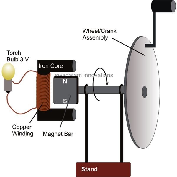
The Dynamo mechanics Figuring
The Real Dynamo Mechanics
Automatic Bicycle Dynamo Mechanics
The circuit works totally automatic, in the day time the circuit will switch off the LED and automatically connect the dynamo with the charger circuit so while you are on your ride it charges the 6V
4.5AH battery that will store a quite good amount off power so you can use this power for charging and powering your variety of devices.
When the battery will become fully charged the circuit will automatically disconnect it with the dynamo and switches ON the LED2 that shows the indication of battery full charged. Due to this automatic function your battery will not overcharge and works for a long time. In the night time the circuit automatically switches the dynamo to the 12V 6W LED.
The circuit requires some adjustments for the first time for this purpose you require a variable power supply. After building the circuit first of all remove the dynamo supply with its 4 diodes which from D1-D4 and connect a 12V power supply DC with the circuit. Now cover the LDR with a black solution tape and adjust the 50K variable resistor until the 6W LED switches ON. Now remove the 6V 4.5AH battery from the circuit and set 7.3V in the variable power supply and connect it in the place of the 6V 4.5AH battery and adjust the 100K variable resistor until the LED2 goes ON.
After these adjustments remove the black solution tape from the LDR and connect the dynamo with the circuit and also the 6V 4.5AH battery. For best results fix the circuit in a suitable enclosure and enclose the LDR in a small tube attached with the enclosure so the LDR only receive the day light and not the light of other vehicles and street lights

A bicycle dynamo output can be used to power variety of devices, in this article we are discussing about DIY bicycle USB charger circuit that will use the output power of your bicycle dynamo and produces a regulated 5V output to charge your devices which require 5V charging input for example . your smartphones, cameras, mp3, mp4, GPS etc.
The circuit is easy to build and requires only few components. A 6V 3W dynamo is used in the circuit but you can also connect the circuit with a 12V dynamo. If you want to use the circuit with a 12V dynamo just change the voltage value of the 2200uF capacitor from 16V to 25V. A female USB socket (Type A) should be connected at the output of the circuit from that you could connect your devices.

Dynamo Circuit Diagram

Dynamo Circuit Diagram welcome to be able to the blog site, within this time I am going to explain to you with regards to Dynamo Circuit Diagram. And today, here is the very first picture, dynamo circuit diagram, bicycle dynamo circuit diagram, dynamo torch circuit diagram, ac dynamo circuit diagram, dynamo generator circuit diagram, bike dynamo circuit diagram :


Bicyle Light: Cycle Dynamo

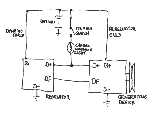
The circuit is 6V, 3W dynamo compatible and its working is very simple and straightforward. When the bicycle dynamo is idle, it connects the light source to the reservoir battery pack until the dynamo starts generating voltage again. The circuit also prevents the light source against high power when the dynamo is running, and uses the available surplus power to recharge the battery pack.
As the diagram shows, the standard bicycle headlight bulb is replaced with a compact 1W generic white LED module. Likewise, the tail lamp is replaced with a 10mm red LED. The battery pack is a combination of five 1.2V, 600mAh Ni-Cd cells, connected in series to produce an output of 6V DC.
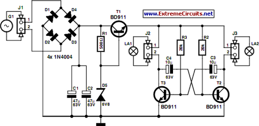
When you ride the bicycle, the dynamo touching the wheel spins around and diodes D1, D2, D3 and D4 form a bridge via which buffer capacitor C1 charges. When the dynamo voltage is sufficiently high, the low-current 5V relay energises and the DC supply available across C1 is routed to the head lamp (LED1) driver circuit (and to the tail lamp LED) through power switch S1. At the same time, the Ni-Cd battery pack charges through components D5 and R1.
When the bicycle is not driven and the dynamo is standstill, the relay is no longer energised. Therefore the bicycle lights (LED1 and LED2) are powered by the Ni-Cd battery pack. Diode D5 prevents the Ni-Cd battery from slowly discharging via the circuit when the bicycle is not used (switch S1 should then be opened).
When white LED is used as the bicycle headlight (with supporting optics), the result is quite good. However, the viewing angle and the brightness of LEDs vary inversely. A wider angle will result in lower brightness in any given direction as the total light output of the LED is spread over a larger area. For headlight applications, a 20° viewing angle is appropriate. This narrow beam aspect of many of the white LEDs has a downside too. The narrower the LED beam, the dimmer it will appear when viewed off angle!
As shown in the circuit diagram, the headlight unit includes a 1W white LED and a small driver section. The driver section is, in fact, a constant-current driver realised using medium-power npn transistor BD139 (T1). The charger jack (J1) allows you to recharge the Ni-Cd battery pack with the help of an external DC power source such as a travel charger (9V) or a miniature solar panel (6V). The 12V zener diode (ZD1) in the circuit is added deliberately to protect the entire electronics (excluding the external charger) from an accidental over-voltage condition that may occur when the dynamo is running very fast.
Note. Bicycle dynamos are alternators equipped with permanent magnets. These are typically clawpole generators delivering energy at rather low RPM. The sidewall-running dynamo (aka bottle dynamo) is the most popular type.
Most bicycle dynamos are rated 6V, 3W (500 mA at 6V). However, the power of a dynamo light system depends somewhat on the speed. In a standard bicycle light system, the power is zero at standstill. At moderate speed it’s about 3W, and at very high speed it’s just a little more than 3W.
 Fig. 1: Circuit for smart bicycle light Fig. 1: Circuit for smart bicycle light |
When you ride the bicycle, the dynamo touching the wheel spins around and diodes D1, D2, D3 and D4 form a bridge via which buffer capacitor C1 charges. When the dynamo voltage is sufficiently high, the low-current 5V relay energises and the DC supply available across C1 is routed to the head lamp (LED1) driver circuit (and to the tail lamp LED) through power switch S1. At the same time, the Ni-Cd battery pack charges through components D5 and R1.
When the bicycle is not driven and the dynamo is standstill, the relay is no longer energised. Therefore the bicycle lights (LED1 and LED2) are powered by the Ni-Cd battery pack. Diode D5 prevents the Ni-Cd battery from slowly discharging via the circuit when the bicycle is not used (switch S1 should then be opened).
 Fig. 2: Suggested enclosure |
As shown in the circuit diagram, the headlight unit includes a 1W white LED and a small driver section. The driver section is, in fact, a constant-current driver realised using medium-power npn transistor BD139 (T1). The charger jack (J1) allows you to recharge the Ni-Cd battery pack with the help of an external DC power source such as a travel charger (9V) or a miniature solar panel (6V). The 12V zener diode (ZD1) in the circuit is added deliberately to protect the entire electronics (excluding the external charger) from an accidental over-voltage condition that may occur when the dynamo is running very fast.
Note. Bicycle dynamos are alternators equipped with permanent magnets. These are typically clawpole generators delivering energy at rather low RPM. The sidewall-running dynamo (aka bottle dynamo) is the most popular type.
Most bicycle dynamos are rated 6V, 3W (500 mA at 6V). However, the power of a dynamo light system depends somewhat on the speed. In a standard bicycle light system, the power is zero at standstill. At moderate speed it’s about 3W, and at very high speed it’s just a little more than 3W.
Bike Battery Charger Circuit Diagram
Bicycle Dynamo Battery Charger Circuit Electronic


Build a Bicycle generator


This project consists of a bicycle, which when pedaling by means of a transmission belt, we turn an alternator, transforming the mechanical energy into electrical energy. The bike-generator project is specifically designed and built to convert the movement of bike wheels into electricity. It can be used for the lighting system of the bicycle, to charge the battery of the mobile and, best of all, to charge its own internal and removable battery.
Objective:
converting the mechanical energy of the movement of the wheel of a bicycle into electrical energy by means of a transmission belt and an automobile alternator, once this is done, it is intended to store said energy in order to be used in some electrical device.
Scope:
Transform the mechanical energy into an electric one and then to be used this, by means of the transport in the proposed bicycle.
CHARACTERISTICS
What do bicycles allow us?
Bicycles allow us to easily move from one place to another thanks to human energy. There are also many benefits for health and the environment. Bicycles also allow us to take advantage of human energy to start up various types of machines.
Bicycle system power generator:
This system of energy generating bicycles, called Hybrid 2, is able to obtain it in two ways that of all life that is produced thanks to pedaling, and the newest, thanks to the regenerative braking system "hybrake", a very similar system to which nowadays they use other means of sustainable transport.
Materials:


Bike
Tripod
Alternator
Car battery
Back support
Cables
Power inverter
Belt or alternator belt

XO__XO Dynamo DB: Replication and Partitioning Application
Computer Networking in Earth

partitioning and replication.
Partitioning in DynamoDB
As mentioned earlier, the key design requirement for DynamoDB is to scale incrementally. In order to achieve this, there must be a mechanism in place that dynamically partitions the entire data over a set of storage nodes. DynamoDB employs consistent hashing for this purpose. As per the Wikipedia page, “Consistent hashing is a special kind of hashing such that when a hash table is resized and consistent hashing is used, only
K/n keys need to be remapped on average, where K is the number of keys, and n is the number of slots. In contrast, in most traditional hash tables, a change in the number of array slots causes nearly all keys to be remapped.”
Consistent Hashing (Credit)
Let’s understand the intuition behind it: Consistent hashing is based on mapping each object to a point on the edge of a circle. The system maps each available storage node to many pseudo-randomly distributed points on the edge of the same circle. To find where an object
The basic implementation of consistent hashing has its limitations:
O should be placed, the system finds the location of that object’s key (which is MD5 hashed) on the edge of the circle; then walks around the circle until falling into the first bucket it encounters. The result is that each bucket contains all the resources located between its point and the previous bucket point. If a bucket becomes unavailable (for example because the computer it resides on is not reachable), then the angles it maps to will be removed. Requests for resources that would have mapped to each of those points now map to the next highest point. Since each bucket is associated with many pseudo-randomly distributed points, the resources that were held by that bucket will now map to many different buckets. The items that mapped to the lost bucket must be redistributed among the remaining ones, but values mapping to other buckets will still do so and do not need to be moved. A similar process occurs when a bucket is added. You can clearly see that with this approach, the additions and deletions of a storage node only affects its immediate neighbors and all the other nodes remain unaffected.The basic implementation of consistent hashing has its limitations:
- Random position assignment of each node leads to non-uniform data and load distribution.
- Heterogeneity of the nodes is not taken into account.
To overcome these challenges, DynamoDB uses the concept of virtual nodes. A virtual node looks like a single data storage node but each node is responsible for more than one virtual node. The number of virtual nodes that a single node is responsible for depends on its processing capacity.
Replication in DynamoDB
Every data item is replicated at
N nodes (and NOT virtual nodes). Each key is assigned to a coordinator node, which is responsible for READ and WRITE operation of that particular key. The job of this coordinator node is to ensure that every data item that falls in its range is stored locally and replicated to N - 1nodes. The list of nodes responsible for storing a certain key is called preference list. To account for node failures, preference list usually contains more than N nodes. In the case of DynamoDB, the default replication factor is 3.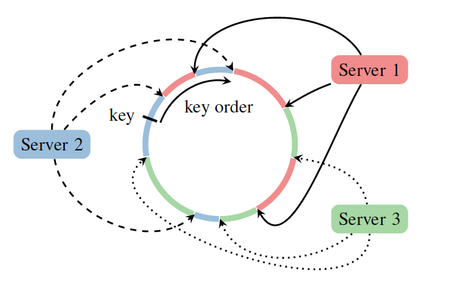

Computer networks - In telecommunications networks, a node (Latin nodus, 'knot') is either a redistribution point or a communication endpoint. ... A physical network node is an active electronic device that is attached to a network, and is capable of creating, receiving, or transmitting information over a communications channel.
(1) In networks, a processing location. A node can be a computer or some other device, such as a printer. Every node has a unique network address, sometimes called a Data Link Control (DLC) address or Media Access Control (MAC) address. (2) In tree structures, a point where two or more lines meet.
A node is any physical device within a network of other devices that's able to send, receive, and/or forward information. ... For example, a network connecting three computers and one printer, along with two other wireless devices, has six total nodes. Any system or device connected to a network is also called a node. For example, if a network connects a file server, five computers, and two printers . A node can be a couple of different things depending on whether the conversation is about computer science or networking. Everything sending, receiving or forwarding traffic. A “network” is a set of “links” and “nodes”. Just like edges and vertices in a graph. In data communication, a node is any active, physical, electronic device attached to anetwork. These devices are capable of either sending.
computer Networking
In its most basic form, a network is two or more computers that are connected with a communications line for purposes of sharing resources. so, if two computers connect to each other over a telephone line or through a piece of cable or even through a wireless connection and the users are able to access ad share files and peripheral devices on the other computers, a network is formed. the individual systems must be connected through a physical pathway (called the transmission medium). All systems on the physical pathway must follow a set of common communication rules for data to arrive at its intended destination; and for the sending and receiving systems to understand each other. The rules that govern computer communication are called protocols.

Networking must have the following:
- Something to share (data)
- A physical pathway (transmission medium)
- Rules of communication (protocols)
System design interview
Consistent hashing is a simple yet powerful solution to a popular problem: how to locate a server in a distributed environment to store or get a value identified by a key, while handle server failures and network change?
A simple method is number the servers from 0 to N – 1. To store or retrieve a value V, we can use
Hash(V) % N to get the id of the server.
However, this method does not work well when 1) some servers failed in the network (e.g, N changes) or 2) new machines are added to the server. The only solution is to rebuild the hash for all the servers, which is time and resource consuming Given that failures are common with a network with thousands of machines, we need a better solution.
Consistent hash
Consistent hash is the solution to the above described problem. In consistent hash, the data and the servers are hashed to the same space. For instance, the same hash function is used to map a server and the data to a hashed key. The hash space from 0 to N is treated as if it forms a circle- a hash ring. Given a server with
IPX, by applying the hash function, it is mapped to a position on the hash ring. Then for a data value V, we again hash it using the same hash function to map it to some position on the hash ring. To locate the corresponding server we just move round the circle clockwise from this point until the closest server is located. If there is no server found, a first server will be used. This is how to make the hash space as a ring.
For example, in the following figure, A, B, C, D are servers hashed on the ring.
K1 and K2 will be served by B. K3 and K4 will be served by C.
One problem of this method is that some servers may have disproportionately large hash space before them. This will cause these servers suffer greater load while the remainder servers might serve too few data. A solution is to create a number of virtually replicated nodes at different positions on the hash ring for each server. For example, for server A with ip address
IPA, we can map it to M positions on the hash ring using Hash(IPA + "0"), Hash(IPA +"1"), … Hash(IPA +"M - 1").
This can help the servers more evenly distributed on the hash ring. Note that this is not related to server replication. Each virtual replicated position with
Hash(IPA + "x") represents the same physical server with IP address IPA.
In the following figure, server A has four virtual nodes on the ring. We can see that the physical servers can handle data more proportionally.

consistent hash virtual node
Implementation of Consistent hash
The following is the implementation of Consistent hash using Java.
1
2
3
4
5
6
7
8
9
10
11
12
13
14
15
16
17
18
19
20
21
22
23
24
25
26
27
28
29
30
31
32
33
34
35
36
37
38
39
40
41
42
43
44
45
46
47
48
49
50
51
52
53
54
55
56
57
58
59
|
import java.util.Collection;
import java.util.SortedMap;
import java.util.TreeMap;
interface HashFunction {
public int hash(Object key);
}
interface Server{
public String getName();
public void setName(String name);
}
public class ConsistentHash<T extends Server> {
private final HashFunction hashFunction;
private final int numberOfReplications;
private final SortedMap<Integer, T> hashRing = new TreeMap<Integer, T>();
public ConsistentHash(HashFunction hashFunc,
int numberOfReplications, Collection<T> servers) {
this.hashFunction = hashFunc;
this.numberOfReplications = numberOfReplications;
for (T server : servers) {
add(server);
}
}
public void add(T serverNode) {
for (int i = 0; i < numberOfReplications; i++) {
hashRing.put(hashFunction.hash(serverNode.getName() + i),
serverNode);
}
}
public void remove(T serverNode) {
for (int i = 0; i < numberOfReplications; i++) {
hashRing.remove(hashFunction.hash(serverNode.getName() + i));
}
}
public T get(Object key) {
if (hashRing.isEmpty()) {
return null;
}
int hash = hashFunction.hash(key);
if (!hashRing.containsKey(hash)) {
SortedMap<Integer, T> tailMap =
hashRing.tailMap(hash);
hash = tailMap.isEmpty() ?
hashRing.firstKey() : tailMap.firstKey();
}
return hashRing.get(hash);
}
}
|
Here we use Java SortedMap to represent the hash ring. The keys for the sorted map are hashed values for servers or data points. The HashFunction is an interface defining the hash method to map data or servers to the hash ring. The
numberOfReplications is used to control the number of virtual server nodes to be added to the ring.
A few points to note:
- The default hash function in java is not recommended as it is not mixed well. In practice, we need to provide our own hash function through the HashFunction interface. MD5 is recommended.
- For Server interface, I only define Name related methods here. In practice, you can add more methods to the Server interface.
Google's TensorFlow is a popular platform that is able to perform distributed training of machine learning/deep learning applications. In this post, I will present several ways of performing distributed training with TensorFlow, especially data parallel and model parallel training. By distributed training, I mean the training process run on multiple devices, especially multiple nodes/machines.
About data parallelism and model parallelism:
Distributed training comes into play as a solution to deal with big data and big model problem. Distributed training enhances the degree of parallelism. Usually, there are two kinds of parallelism in distributed training with Tensorflow: data parallelism and model parallelism. For more explanation: Please refer to this Quora answer What is the difference between model parallelism and data parallelism?
About parameter server concept:
TensorFlow introduces the abstraction of "parameter server" or "ps" from its predecessor DistBelief. Other platforms like MXnet, Petuum also have the same abstraction. Basically, parameter server (ps) is a collection of computing unit (such as device, node and application process) that is responsible for storing and updating the parameters of a machine learning/deep learning model. As a common way to handle mutable state (model parameters), most of the distributed machine learning/deep learning platforms support parameter server functionality.
I am assuming you have basic understanding of Tensorflow and I will omit basic concept/ knowledge about Tensorflow. The following shows the ways we can implement distributed training with TensorFlow:
Some notes:
1, each worker task is responsible for estimating different part of the model parameters. So the computation logic in each worker is different from other one else.
2, There is application-level data communication between workers.
The following Fig 3 shows a model parallel training example:
This example shows how to use model parallel to train a neural network (with three hidden layers) with back-propagation algorithm. (Here is a wonderful tutorial for understanding back-propagation algorithm) There are four computing units (here four worker nodes). Each worker is responsible for storing and updating a subset of the network parameters. In the forward phase (blue arrow), each worker passes the activations to its successor worker. And in the backward phase (red arrow), each worker passes the "error" to its predecessor worker. Once a worker receives the errors from its successor worker, it is ready to update its corresponding parameters. It's worth meaning that in this model parallel scheme, workers are not able to perform computation simultaneously, as a worker can not get starting computing until it receives the necessary stuff, either activations or errors, from its neighbor.


e- Dynamo Virtual


About data parallelism and model parallelism:
Distributed training comes into play as a solution to deal with big data and big model problem. Distributed training enhances the degree of parallelism. Usually, there are two kinds of parallelism in distributed training with Tensorflow: data parallelism and model parallelism. For more explanation: Please refer to this Quora answer What is the difference between model parallelism and data parallelism?
About parameter server concept:
TensorFlow introduces the abstraction of "parameter server" or "ps" from its predecessor DistBelief. Other platforms like MXnet, Petuum also have the same abstraction. Basically, parameter server (ps) is a collection of computing unit (such as device, node and application process) that is responsible for storing and updating the parameters of a machine learning/deep learning model. As a common way to handle mutable state (model parameters), most of the distributed machine learning/deep learning platforms support parameter server functionality.
I am assuming you have basic understanding of Tensorflow and I will omit basic concept/ knowledge about Tensorflow. The following shows the ways we can implement distributed training with TensorFlow:
 |
| Fig 1 |
- Data Parallelism:
Example 1 (Figure 1):
Each worker node (corresponding to a worker task process) executes the same copy of compute-intensive part of the TensorFlow computation graph. Model parameters are distributed/divided into multiple PS nodes(corresponding to ps task processes). There is a separate client for each worker task. In each iteration of training, each worker task takes into a batch of training data and performs computation(e.g. compute the gradient in SGD training) with the model parameters fetched from PS. The resulting gradients from each worker task are aggregated and applied to PS in either sync or async fashionSome notes:
1, In this scheme, the PS only contains a single copy of the model. However, the single copy of the model parameters can be split on different nodes.
2, This scheme can achieve both synchronous and asynchronous training.
3, This is a typical data parallelism training scenario, because in each iteration, each worker performs the same computation logic and has to accommodate the whole model parameters for computation. However, each worker only needs to hold a subset of the training data for each iteration's computation.
4, There is no application-level data (e.g. parameters or activations) communication among workers.
5, The example employs between-graph replication training mechanism. A similar scheme is in-graph replication training, "in-graph" means their is only a single client in the training cluster and the copies of compute-intensive part are within the single computation graph built by the single client. In-graph replication training is less popular than between-graph replication training.
For more information about between-graph replication training, please refer to the tutorial.
Example 2 (Fig 2)
In example 1, I am assuming each computing node in the cluster only contains CPU device. With GPU-powered nodes, the data parallel distributed training might be as the following example 2 ( Fig 2) (You can find this figure here) :
In example 1, I am assuming each computing node in the cluster only contains CPU device. With GPU-powered nodes, the data parallel distributed training might be as the following example 2 ( Fig 2) (You can find this figure here) :
 |
| Fig 2 |
Example 2 shows a single node (with one CPU and two GPUs)'s view of data parallel distributed training. Each GPU executes a worker task. The difference between this example and the previous one is: in example 2 each node's the CPU first aggregates the gradients from all the local GPUs and then applies the aggregated gradients to PS. The fetching of parameters from PS is done by each node's CPU and the CPU then copies the parameters to local GPUs.
You can find code examples for data parallel distributed training on my github: code examples of distributed training with TensorFlow
You can find code examples for data parallel distributed training on my github: code examples of distributed training with TensorFlow
- Model Parallelism
1, each worker task is responsible for estimating different part of the model parameters. So the computation logic in each worker is different from other one else.
2, There is application-level data communication between workers.
The following Fig 3 shows a model parallel training example:
 |
| Fig 3 |
This example shows how to use model parallel to train a neural network (with three hidden layers) with back-propagation algorithm. (Here is a wonderful tutorial for understanding back-propagation algorithm) There are four computing units (here four worker nodes). Each worker is responsible for storing and updating a subset of the network parameters. In the forward phase (blue arrow), each worker passes the activations to its successor worker. And in the backward phase (red arrow), each worker passes the "error" to its predecessor worker. Once a worker receives the errors from its successor worker, it is ready to update its corresponding parameters. It's worth meaning that in this model parallel scheme, workers are not able to perform computation simultaneously, as a worker can not get starting computing until it receives the necessary stuff, either activations or errors, from its neighbor.
From photons to big-data applications: terminating terabits
Computer architectures have entered a watershed as the quantity of network data generated by user applications exceeds the data-processing capacity of any individual computer end-system. It will become impossible to scale existing computer systems while a gap grows between the quantity of networked data and the capacity for per system data processing. Despite this, the growth in demand in both task variety and task complexity continues unabated. Networked computer systems provide a fertile environment in which new applications develop. As networked computer systems become akin to infrastructure, any limitation upon the growth in capacity and capabilities becomes an important constraint of concern to all computer users. Considering a networked computer system capable of processing terabits per second, as a benchmark for scalability,. We seeks to reduce costs, save power and increase performance in a multi-scale approach that has potential application from nanoscale to data-centre-scale computers.
The rapid growth and widespread availability of high-capacity networking has meant that all computers are networked and have become integral to today's modern life. From the appliances we each have in our house and office through to the high-performance computers (HPCs) of weather forecasting to the rise of the data centre, providing our favourite search engine, storage for our family photos and pivot for much corporate, government and academic computing. The modern application presumes network connectivity and increasingly the common application presumes high-performance network connectivity to ensure the timely working of each network operation.
Such demand has been central, driving both the need for networking and the approach towards the capacity crunch (see other publications in this discussion meeting issue). A capacity crunch that has forced photonics development and triggered, with its lower cost of repair, (gigabit) fibre to premises to become the premier standard for Internet new entrants (e.g. Google Fiber) and incumbents (e.g. Comcast and AT&T.)
Cloud usage has driven network demand, yet the cloud itself is not well defined; a cloud may equally likely be provisioned by a company as a subscription service itself or provided as a loss leader. Cloud-based services may present as one or more of a provision of storage, of computing resource or of specific services (e.g. database, Web-based editor). Early cloud incarnations were driven to lower capital costs by centralizing resources and based upon arrays of commodity hosts. However, cloud provision has certainly entered the adolescent years and, with operational costs of electricity and maintenance eclipsing those of provision, effective cloud facilities are bespoke designs that only resemble in computer architecture the commodity boxes of their ancestry. Because few organizations can do custom design and build, the cost to install a cloud system has risen dramatically as scale-out hyper-data centres recoup investment in the bespoke design and manufacture process.
In contrast with Cloud—an offering of services both physical and virtual—for the purposes of the discussion in this paper, the data centre is the physical manifestation of equipment whose purpose is to provide cloud services. The data centre, from the modest physical equipment provisioned within a small department machine-room to the hyper-data centres of Google, Microsoft and Facebook, represents the equipment—computers, storage and networking—upon which cloud services operate.
Cloud-centred network applications include content distribution, e.g. NetFlix and BBC iPlayer, and the more traditional Web services of commerce, targeted advertising and social networking
These sit alongside the wide range of crucial applications yet run sight-unseen supporting specialist use in engineering, science, medicine and the arts. Examples include: jet turbine modelling, car safety simulations and quantitative research as well as sophisticated image processing common to both medicine and the arts as movie post-production processing is now commonplace. All of this is quite aside from the network applications that support our personal communications and interactions with national security.
The effect of high-performance network applications is reflected in the increasing need for network bandwidth. Cisco's Global Cloud Index for 2013–2018 forecasts that global data-centre IP traffic will nearly triple (2.8-fold) over the next 5 years, and that overall data-centre workloads will nearly double (1.9-fold). For current applications, the physical server workload is predicted to rise by 44% for cloud data centres and 13.5% for other, traditional, data centres. Also, new technologies, such as the Internet of Things, will further increase the demand on networking, compute and storage resources, growing the associated data by 3.6-fold by 2018 . Alongside this an expected global consumer storage requirement of 19.3 exabyte (annually) by 2018 suggests current computing architectures do not provide an answer to forthcoming challenges.
While the move to cloud-based computing may improve performance, and reduce operational costs such as power consumption, it does not solve these challenges: the power consumption is not eliminated—rather it is centralized within the data centre, and new networking traffic (that did not exist before migrating to the cloud) is generated between the user and the cloud. Furthermore, the cloud is not always suitable: from researchers in academic institutes to people concerned with their privacy in the post-Snowden era , many require their servers on site. Chen & Sion showed that moving to the cloud is not always cost-effective, as appropriate cloud services are not provided for free, and depend on the skills and particulars of both the users and the applications. Even for those wishing to migrate to the cloud, yet who have only modest network requirements for each application, e.g. download speeds of up to 2.5 Mbps or a latency of up to 160 ms, such a change would currently be impossible on the existing network infrastructure of most countries .
Into this lacuna we propose our alternative, Computer as Network (CAN). Before we justify our approach, in § we describe the needs of several modern applications.
A common misconception is that the storage and processing resources of a centralized cloud data centre will suffice. Yet, just as we have communication and transportation infrastructure across continents deployed at varying scales and for varying needs (e.g. a four-lane interchange on a motorway versus a mini-roundabout in a rural area), so too do we need computing as an infrastructure.
Focused beyond data centres, we outline several use-cases for specific and dedicated computing infrastructure. The effect of latency, the desire for privacy and local control, and the need for availability—each motivate an infrastructure of computing provision. Just as in other types of infrastructure, there is a scaling of resources: from an unpaved road to the motorway (transportation) and from a home landline to a backbone network (communication). It is within this range of computing infrastructures that a lacuna exists: we currently step from a data centre handling petabytes per second of information to commodity servers that only handle gigabytes of data. Figure 1 depicts several use-cases that benefit from computing as an infrastructure.
Figure 1.
Scaling computing infrastructure: from personal computing and personal data centre to tier-1 data centres. (Online version in colour.)
Despite apparent sufficiency, the current arrangement of computers, networks and data-centre services cannot easily effect end-host latency, meet the desire for privacy and local control, or meet the need for availability. Meeting these needs, the personal data centre, suggested by Databox , specifically seeks to provide high availability, and local data-management and privacy controls. With sufficient computing resource, and continued advances in homomorphic encryption , a Databox concept could provide near perfect encryption—allowing computation by third-party services without any privacy concern.
Such sharing becomes critical as, in the manner of power and communications infrastructure, the personal data centre can serve more than a single household. Just as consumers are already familiar with being paid for returning excess solar-panel production to the grid, personal data-centre services could be provided in a similar way. The owner of a personal data centre could, just as some British Telecom users share their home wireless and extend their wireless coverage through other participating consumers' equipment, share resources from their personal data centre among other similarly minded contributors. A personal data centre that allows sufficient resource control, moderation and security is an important enabling technology.
Mobile computing has provided the spearhead use-case for cloud-based computation. It lowers handset power consumption and maximizes battery life by offloading computations. However, conducting most of the computations off the mobile device is combined with a need for a crisp user experience that requires low latency. Cloudlets have been proposed to address the latency needs for mobile-device offload. A Cloudlet is a trusted, resource-rich, computer that is both well connected to the Internet and available for use by nearby mobile devices. Cloudlets are an interim computing level between mobile devices and full cloud services, but they also require powerful local computing. This local computing resource needs to support isolation between a large number of users. Cloudlets also require considerable processing resources in order to both offload mobile computations and provide a satisfying user experience.
Regardless of their size, enterprises are very sensitive to their computing infrastructure. Almost any company today requires significant computing resources and many are encouraged to move their computing and storage to the cloud—to data-centre services owned by other companies. Such moves may not be appropriate: a legal company has certain confidentiality constraints that force data to be on company premises, or a video post-production house must simultaneously manipulate dozens of 50 Gbps (8 k video) data streams. In each of these companies, commodity servers are insufficient for their growing needs, yet moving workloads to the cloud adds too much latency, is too expensive or is illegal. An enterprise must seek a solution that provides the high performance, reliability and resilience required for its needs, but also the ability to maintain physical access and to support the computer: that is, support a large number of users with different sets of policies, and be able to monitor their activities, debug problems and recover from failures.
Research projects where data must be physically co-located with measurement apparatus, or where it is not practical to move data to a remote facility, share much in common with the enterprise case. Furthermore, despite growing research budget pressures, research computing needs continue to grow. We offer a roadmap to high performance and strong isolation that is perfect for sharing common facilities.
The need for smaller data-centre facilities nearby to users has not escaped the notice of the larger data-centre cloud operators; and they also have a need for tiers of smaller data centres deployed closer to users. Such deployments of many thousands of small data centres at the edge of their networks further supports our need-based uses.
In the last decade, a revolution in computing concepts has occurred. Alas, most efforts have focused upon the economy of scale, exploiting cost advantages by expanding the scale of production. This puts data-centre computing at the focus of interest. To name just a few of these efforts, Firebox is an architecture containing up to 10 000 compute nodes, each containing about 100 cores, and up to an exabyte of non-volatile memory connected via a low-latency, high-bandwidth optical switch. Firebox is focused on designing custom computers using custom chips. HP's The Machine focuses on flattening the memory hierarchy using memristor-based non-volatile memory for long-term storage. The Machine also uses a photonic interconnect to provide both good latency and high bandwidth among sub-systems. This wholesale use of new technologies that provide a near-flat latency interconnect and widely available persistent memory has a large impact upon any software. Both Firebox and The Machine look at data-centre-scale computing that has requirements different from a collection of co-located servers, and thus their designs require a holistic approach that treats the entire system as a single machine . However, the complexity of these new machines and immaturity of the new technologies led to limited applicability and a longer time for adoption.
Another approach that exploits the economies of scale by using commodity components is represented by RackScale and the Open Compute project . The RackScale architecture is usually referred to by three key concepts : the disaggregation of the compute, memory and storage resources; the use of silicon photonics as a low-latency, high-speed fabric; and, finally, a software that combines disaggregated hardware capacity over the fabric to create ‘pooled systems’. The Open Compute project is an open source project that seeks to design the most efficient server, storage and data-centre hardware for data-centre computing. Here every element in the data centre is based on customized boxes built around commodity components and open source software, and cannot be considered to revolutionize computing concepts. Rack scale is not well defined, it can refer to a large unit, filling part of a rack; it may also refer to a single rack ; and it sometimes also refers to a small number of racks .
Several commercial products have tried to address the growing computing needs. Examples include HP's Moonshot and AMD's Seamicro . These machines range in size from one to 10 rack units (being a quarter of a full rack), and sometimes contain more than 1000 cores, divided between many small server units. Unfortunately, none of these products provides a long-lasting scalable solution, as shown by HP replacing the Moonshot architecture with The Machine, and SeaMicro being cancelled by AMD .
Specialist HPC applications have driven a set of requirements disjoint from personal or cloud computing. These expensive single-application systems target very different types of applications and thus are outside the scope of this work.
Limitations of current-day architectures
The computing industry historically relied on increased microprocessor performance as transistor density doubled , while power density limits ] led to multi-processing . Common servers today consist of multiple processors, each consisting of multiple cores, and increasingly a single machine runs a hypervisor to support multiple virtual machines (VMs). A hypervisor provides to each VM an emulation of the resources of a physical computer. Upon each VM, a more typical operating system and application software may operate. The hypervisor allocates each VM memory and processor time. While a hypervisor gives access to other resources, e.g. network and storage, limited guarantees (or constraints) are made on their usage or availability.
While VMs are popular, permitting consolidation and increasing the mean utilization of machines, the hypervisor has limited ability to isolate competing resource use or mitigate the impact of usage between VMs. Beyond predictability, this also limits robustness, as machines are sensitive to the mix of loads running on top of them. Resource isolation has been the focus of considerable research over the years, with examples from the multi-processor set-up to resource isolation between VMs (e.g. ). Work on precise hardware communication-resource allocation has been limited in scalability or has been carried out as thought-experiments (e.g. ).
Resource isolation is not the only challenge for scaling computing architectures. General purpose central processing units (CPUs) are not designed to handle the high packet rates of new networks. Doing useful work on a 100 Gbps data stream exceeds the limits of today's processors. This is despite the modern CPU intra-core/cache ring-bus achieving a peak interface rate of 3 Tbps , and a peak aggregate throughput that grows proportionally with the number of cores. Unlike networking devices, CPUs may spend many instruction cycles per packet. Even the best current networking driver requires over 100 cycles to send or receive a packet; doing useful work is even more cycles: an application accessing an object on a small (8 Mbyte) list structure requires at least 250 cycles . A data stream of 100 Gbps, with 64 byte packets, is a packet rate of 148.8 M packets per second; thus a 3 GHz CPU has only 20 cycles per packet: significantly less than required even just to send or receive. The inefficiency of packet processing by the CPU remains a great challenge, with a current tendency to offload to an accelerator on the network interface itself .
In-memory processing and the use of remote direct memory access as the underlying communications system is a growing trend in large-scale computing. Architectures such as scale-out non-uniform memory access (NUMA) for rack-scale computers are very sensitive to latency and thus have latency-reducing designs . However, they have limited scalability due to intrinsic physical limitations of the propagation delay among different elements of the system. A fibre used for inter-server connection has a propagation delay of 5 ns/m; thus, within a standard height rack, the propagation delay between the top and bottom rack units is approximately 9 ns, and the round-trip time to fetch remote data is 18 ns. While for current generation architectures this order of latency is reasonable , it indicates scale-out NUMA machines at data-centre scale (with each round-trip taking at least 1 μs) are not plausible, as the round-trip latency alone is many magnitudes the time-scale for memory retrieval off local random access memory or the latency contribution of any other element in the system. With latencies aggressively reduced across all other elements of in-memory architectures, such propagation delays set a limit on the physical size and thus the scalability of such an architecture.
Photonics has advanced hand in hand with network-capacity growth. However, photonics has its own limitations : the minimum size for photonic devices is determined by the wavelength of light, e.g. optical waveguides must be larger than one-half of the wavelength of the light in use. Yet, this is over an order of magnitude larger than the size of complementary metal-oxide semiconductor transistors. Consequently, the miniaturization of photonic components faces fundamental limits and photonic device sizes cannot be continuously scaled in physical dimensions. Furthermore, unlike electronic devices in which the signals are regenerated at each sequential element, optical loss, crosstalk and noise build up along a cascade of optical devices, limiting scalability of any purely optical path.
Limitations are faced at several levels in the system hierarchy: from the practical limitations of physics to the increasing impedance mismatch between processor clock speed and network data rates. We have not even discussed the limitations of economics and politics that mean both large and low-latency (closed) data-centre facilities are rarely plausible: there is no practical real estate for a large data centre within the M25 orbital of London, UK, even if it were politically desirable. As a result, we motivate our own work to address a range of limitations from the impact of bandwidth, the desire to reduce application latency and also to be a practical and enabling effort: one that allows a decentralization of resources with the attendant advantages that bring forth power, privacy and latency.
The gap between networking and computing
The silicon vendors for both computing and networking devices operate in the same technological ecosystem. CPU manufacturers often had access to the newest fabrication processes and the leading edge of shrinking gate size, while most networking device vendors are fabless, lagging a few years behind in capitalizing on this. Yet, networking devices have shown over the past 20 years superior datapath bandwidth improvement to CPUs . Furthermore, in the past 20 years, the interconnect rate of networking devices doubled every 18 months, whereas computing system I/O throughput doubled approximately every 24 months . At the interface between network and processor PCI-Express, the dominant processor-I/O interconnect, the third generation of which was released in 2010, achieves 128 Gbps over 16 serial links ]. The fourth generation—expected in 2016—aims to double this bandwidth. By contrast, Intel's inter-socket quickpath interconnect (QPI) currently achieves 96 Gbps (unidirectional). Meanwhile, networking interconnects have achieved 100 Gbps and 400 Gbps for several years. Furthermore, these interfaces achieve their high throughput over a smaller number of serial links: four serial links for 100 Gbps and eight serial links for 400 Gbps . The limitations of existing computing interconnects vexes major CPU vendors
General purpose processors are extremely complex devices whose traits cannot be limited to specifications such as datapath bandwidth or I/O interconnect. Subsequently, we evaluate the performance of CPUs using the Standard Performance Evaluation Corporation (SPEC) CPU2006 benchmark and contrast this with the improvement in network-switching devices and computing interconnect. To evaluate the improvement of CPUs, we consider all the records submitted to the SPEC CPU2006 database, for both integer and floating point, speed and throughput benchmarks. For every year, from 2006 to mid-2015, we select the CPU with the highest result—and since SPEC evaluates machines and not CPUs, we do that by dividing the result of each machine by the number of CPU sockets. Figure 2 shows the relative improvement of CPU speed and throughput performance over the years, growing fourfold (integer) and sevenfold (floating point) in speed and about 27-fold in throughput (both floating point and integer). For clarity, we include only integer benchmark performance improvement in the graph
Figure 2.
The relative improvement of computing and networking devices over the last 15 years. (Online version in colour.)
For networking devices, we observe 266-fold improvement in the throughput of standard top-of-rack Ethernet switches from 2002 to 2014 . Finally, between networking and processor, the performance of the PCI-Express interconnect has improved only 6.4-fold from its introduction to the upcoming PCI-Express fourth generation. Aside from the lack-lustre improvements in interconnect standards, the other observation from figure 2 is the rate of change for each measurement. While networking device performance doubles approximately every 18 months and CPU throughput performance doubles every 24 months, the interconnect between CPUs improves at the CPU rate. Over time, we predict this lag in scaling has led to a growing gap in performance between networking and computing devices.
Networking devices have supported the need to actively differentiate traffic. Sophisticated methods for queue control exist so that network operators can deliver over the same physical infrastructure differing network traffic (e.g. video distribution, voice calls and consumer Internet traffic), each with different needs and constraints (e.g. minimal loss, constrained latency or jitter). Effort to support this means that current network silicon support controls millions of individual flows—magnitudes of more than the hundreds or thousands of VMs per host.
One of the topics that has been core to networking devices over the years is providing a predefined quality of service to users. This is what most people know as a service-level agreement (SLA). Today, Internet connectivity, television and phone services are provided to end-users over a shared networking infrastructure, and every user can opt for a different SLA for a different cost. Consequently, networking devices implement in hardware complex schemes that provide the agreed quality of service to a large number of users, such as priorities, committed and excess bandwidth, and support properties such as low latency and bounded jitter. Furthermore, these are supported for hundreds of thousands of different flows, in contrast to the hundreds or thousands of VMs per host commonly supported by VM appliances. Such network service isolation is of sufficient granularity to support the requirements identified in §4.
Not only is energy consumption and dissipation the primary force in CPU design but heat dissipation is important to ensure device performance: the features of devices are dictated by the thermal footprint. In contrast with CPUs, networking devices have managed to avoid complex dissipation systems, using only passive heat-sinks and enclosure fans. Thus, the reliability of networking systems is higher while the electrical operating costs are lower than a typical server.
To bridge the performance gap between networking and computing by capitalizing upon the promise of current networking approaches, we can draw upon the practices of network switch silicon while applying the long-standing principles of stochastic networking . One might envisage a stochastic treatment of transactions permitting an application of certain bounded throughput and latency for each transaction context.
Computer as Network
we present a new computer architecture, dubbed CAN (Computer as Network). This new architecture borrows ideas and practices from the networking world to address the challenges presented by computing.
(a) The CAN architecture
CAN server architecture is focused on multi-core, multi-socket servers and explicitly has a networking fabric at the core of the computing device, as illustrated in figure 3. Key to this proposed architecture is that every I/O transaction among elements in the system is treated. By transaction, we refer to any movement of data over any interconnect within the server; in the CAN we do not differentiate transactions for networking from transactions for I/O devices from transactions for memory or inter-socket communications. In all cases, like the handling of data packets within networks, we can apply performance guarantees such as priorities, throughput guarantees and latency guarantees to each transaction. A side-effect is to minimize cross-talk between any transaction: that is, every I/O operation. This also enables us to use more efficient, network-centric, methods for moving data among the components of a computer architecture.
Figure 3.
Comparative architectures: (a) common commodity four-socket system, (b) proposed CAN concept. In the common commodity system, an I/O channel is associated with a specific dedicated socket. In the CAN concept, all I/O (storage, networking, etc.) is associated with the CAN-D. (Online version in colour.)
Figure 3 illustrates the concept of CAN, contrasting a commodity four-socket architecture with CAN. It is clear in the commodity four-socket architecture that, because I/O systems, network devices, graphics devices, etc., are each associated with a particular socket, any data generated off-socket must hop-by-hop progress through the X–Y grid of sockets, in addition to introducing variable latency; older results show 150 ns variance across an eight-socket system. Such data movement will consume intermediate communications and cache resources as transactions are relayed through the CPU-based network. By contrast, the CAN approach is to use a low-overhead switching element with direct single-hop access to every socket. Even today, standard switching silicon can achieve switching delays of less than 100 ns independently of the port-count or fabric size. Now consider a CAN server in a standard (19-inch) rack width. The server contains several CPU sockets: the number of sockets can comfortably be between two and 12 sockets. This value is derived by realistic server power and space considerations. Each CPU socket is directly connected to the network fabric, which consists in turn of one or more network devices. Alongside the networking and I/O ports, the fabric device, CAN-D (CAN Device), also connects directly to all the peripherals of the server: storage devices, memory devices, graphic processing units (GPUs), etc. Finally, the CAN-D has direct access to a large quantity of its own buffering memory.
Any new transaction arriving to CAN-D, either from within the computer or externally, is mapped to a destination device (which can be any device on board), and to a flow. A flow can be destined to a process of a VM on a core within a particular CPU socket, or any other peripheral device. Each flow is assigned a set of properties, such as committed throughput, absolute priorities and bounding on latency. Each transaction can be guaranteed these properties as it is forwarded to its destination. Low-priority transactions can be stored in the CAN-D buffering, to allow transactions with higher priority to jump the queue and receive priority handling. A common network facility, CAN-D allows a transaction to be trivially sent to multiple destinations (multi-cast); such abilities would provide for easy replication and locking primitives. Finally, the CAN architecture supports multi-controller access to memory devices such as the hybrid memory cube (HMC . Thus, a high-throughput flow can be written directly to the processor's attached memory without crossing the processor's interconnect nor wasting other on-socket resources. All the while, a control channel can be provided in parallel between the CAN-D and the processor, permitting permission controls and pre-emption as required.
CAN is a scale-up architecture, and as such it is important to note that CAN does not cause traffic explosion within the network fabric, as each device within the server generates transactions at a rate equal to its maximal performance, and overall the intra-server communication is designed to be of the same order as the inter-server communication. Intra-server communication scales with networking performance, and CAN-D uses common networking architectures and practices such as local buffering, thus the overall bandwidth for the CAN-D scales with commodity networking devices.
While CAN is focused on the server level, this approach can also be applied at the smaller scale processor level as well as the larger scale data-centre level. On the processor level, CAN-D can be implemented as the fabric between cores (e.g. using a photonic-based fabric layer as the bottom of a three-dimensional die-stack device). On the data-centre level, CAN can be extended to have a top of rack CAN-D or spine CAN-D interconnecting CAN fabrics across multiple servers, racks or pods. In this manner, CAN can scale-out, and not only scale-up.
In our approach, CAN opts for a non-coherent operating model, using operating systems such as Barrelfish or Unikernels . Support for coherency is feasible on CAN, for example to support large-coherency objects, e.g. database applications. This could be achieved by using the priority mechanics of the network fabric. However, for a highly scalable architecture that supports heterogeneous devices, where coherency cannot be supported by hardware, we claim that a software-based approach such as suggested by COSH is better.
The concept of a network fabric as the core of a computer was in part inspired by the Desk Area Network (DAN) , a multi-media workstation that used a single, common, network interconnect among all sub-systems (CPU, memory, network, audio and video I/O devices). It also considers ideas proposed for HPCs, and adapts them to affordable commodity hardware and to computing as infrastructure use-cases.
(b) The benefits of CAN
CAN as a scalable architecture scales with network-switching performance for inter-server transactions, and with computing-interconnect bandwidth for intra-server transactions, using existing commodity devices. The use of CAN-D bridges the performance gap between networking and computing, and provides the first entry on a roadmap for lasting performance improvement. Beyond high throughput, CAN provides the above-mentioned performance guarantees: committed and excess throughput, priorities and bounded latency. Furthermore, CAN-D is designed to support the implementation of new and emerging performance guarantees, in a manner that allows easy adoption.
CAN provides isolation between compute and I/O units, isolating processes and/or VMs as required. The isolation of resources means the completion of a job is predictable, while the computer is robust to interference: the execution time of each job no longer depends on other work running in parallel.
However, the CAN approach also has challenges: by supporting so many individually annotated transactions, the management and maintenance must not be neglected. Scalable solutions from the software-defined network community can be adopted to configure and manage flows of information in our system. We believe that we can also capitalize on the burgeoning network verification and correctness efforts to aid in CAN debugging tools from the earliest design stages.
CAN is an approach to computer architecture, rather than a set definition. As such, the implementation of CAN is flexible. Figure 4 illustrates several different types of implementations of CAN: centralized and distributed network fabric implementations, a centralized memory implementation and an implementation that enables multiple controllers access to memory. This flexibility makes CAN complementary to the data-centre disaggregation trend, as it can operate both as an aggregated and a disaggregated box. CAN uses an interface oblivious design that enables a single CAN-D device with flexible configurations: any single interface may operate as a compute-interconnect, a storage-interconnect or as a network-interconnect. Such flexibility is feasible today, but is typically restricted to a switching hierarchy with several different network types. This flexibility also enables the use of different networking infrastructure for CAN-D: from a standard electrical device to an experimental photonic-based fabric.
Figure 4.
The flexibility of CAN architecture: examples of several different implementation schemes. (a) Centralized network fabric, where all intra-server communication is through CAN-D. (b) Distributed network fabric, where only part of the intra-server communication is through CAN-D. (c) A multi-controller memory implementation, where both CAN-D and CPU devices are attached to the RAM. (d) A centralized memory topology, where all devices access the RAM through CAN-D. The number and type of devices connected to CAN-D vary as well. (Online version in colour.
An interface-oblivious design based upon a photonic fabric and photonic-based interconnects enables scalability in a different dimension: once a CAN box is in operation, it may continuously scale. The optical switch and pathway infrastructure are oblivious to the data rate carried. Thus, a move from a 10 Gbps to 100 Gbps to 1 Tbps per port is a transparent change. The CPU may be upgraded but the I/O interface remains the same speed oblivious of the optical interconnect. This also offers possibilities to reduce costs, and ease the maintenance and upgrade processes.
The CAN architecture is the answer to computing as required by an infrastructure. This is not only because of its high performance and ability to terminate terabits, but also because of the things that matter for infrastructure: scalability, cost, reliability and management. A small CAN-based computer can serve as a personal data centre, a CAN box will provide a cloudlet's local computing infrastructure, and a collection of CAN blades will build the next-generation rackscale-based data centre.
Conclusion
A new architecture for affordable HPCs, using networking practices to bridge the performance gap between the networking and the computing world. This approach is a rethinking of current models; it uses resource control commonly available within networking devices to improve both the performance and efficiency of current computers. An architecture that places networking at the centre of the machine requires a fusion of knowledge from computer systems, network design, operating systems and applications; yet it will provide for a revolution, solving issues forced on servers by current approaches and architectures.
An important part of the success of novel computing architectures has always been a combination of hardware and software contributions. CAN aims to create a close integration between hardware and software, which is essential in order to capitalize on the features provided by the hardware. On the other hand, wide adoption requires as small a number of changes as possible to the application level, otherwise adapting the applications would become too costly (in terms of time and resources). We foresee a prototype of the CAN architecture. We would envisage this based on the NetFPGA SUME open source reconfigurable platform, using the CHERI soft core processor and operating and extending the FreeBSD operating system.
We define our architecture as a call-to-arms, not as the definitive answer to the capacity-crunch in the end-systems but as an enabling force that will mean we can explore practical realization of novel data-centre uses: ones that are optimized to preserve our privacy through disaggregation (§2), an approach that enables a new class of use-cases enabling effective mobile devices ], and as a practical approach to the disaggregated data centre that can both meet our future computational needs and capitalize on the disaggregated energy sources that a large-scale move to renewables (e.g. ]) would entail. However, an architecture alone is not enough to achieve our goals. We foresee a rise in such innovative architectures also enabling new efforts to realize appropriate operating system and application innovations and believe that, irrespective of the absolute correctness of our architecture for every purpose, the innovation opportunities enabled will also have long-lasting consequences.
++++++++++++++++++++++++++++++++++++++++++++++++++++++++++++++++++++++++++++++++++++++
e- virtual dynamo like network data on a computer as like as e- WET dynamo electronic circuit

++++++++++++++++++++++++++++++++++++++++++++++++++++++++++++++++++++++++++++++++++++++
.
Tidak ada komentar:
Posting Komentar