
Belt (mechanical)
A belt is a loop of flexible material used to link two or more rotating shafts mechanically, most often parallel. Belts may be used as a source of motion, to transmit power efficiently or to track relative movement. Belts are looped over pulleys and may have a twist between the pulleys, and the shafts need not be parallel.
In a two pulley system, the belt can either drive the pulleys normally in one direction (the same if on parallel shafts), or the belt may be crossed, so that the direction of the driven shaft is reversed (the opposite direction to the driver if on parallel shafts). As a source of motion, a conveyor belt is one application where the belt is adapted to carry a load continuously between two points.
 A pair of v-belts
 flat belt
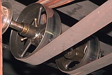
The mechanical belt drive, using a pulley machine, was first mentioned in the text the Dictionary of Local Expressions by the Han Dynasty philosopher, poet, and politician Yang Xiong (53–18 BC) in 15 BC, used for a quilling machine that wound silk fibers on to bobbins for weavers' shuttles.[1] The belt drive is an essential component to the invention of the spinning wheel.The belt drive was not only used in textile technologies, it was also applied to hydraulic powered bellows dated from the 1st century AD .
Power transmission[edit]
Belts are the cheapest utility for power transmission between shafts that may not be axially aligned. Power transmission is achieved by specially designed belts and pulleys. The demands on a belt-drive transmission system are huge, and this has led to many variations on the theme. They run smoothly and with little noise, and cushion motor and bearings against load changes, albeit with less strength than gears or chains. However, improvements in belt engineering allow use of belts in systems that only formerly allowed chains or gears.
Power transmitted between a belt and a pulley is expressed as the product of difference of tension and belt velocity:

where, T1 and T2 are tensions in the tight side and slack side of the belt respectively. They are related as

where, μ is the coefficient of friction, and α is the angle (in radians) subtended by contact surface at the centre of the pulley.
Pros and cons
Belt drives are simple, inexpensive, and do not require axially aligned shafts. They help protect machinery from overload and jam, and damp and isolate noise and vibration. Load fluctuations are shock-absorbed (cushioned). They need no lubrication and minimal maintenance. They have high efficiency (90–98%, usually 95%), high tolerance for misalignment, and are of relatively low cost if the shafts are far apart. Clutch action is activated by releasing belt tension. Different speeds can be obtained by stepped or tapered pulleys.
The angular-velocity ratio may not be constant or equal to that of the pulley diameters, due to slip and stretch. However, this problem has been largely solved by the use of toothed belts. Working temperatures range from −31 °F (−35 °C) to 185 °F (85 °C). Adjustment of center distance or addition of an idler pulley is crucial to compensate for wear and stretch.
Flat belts

Flat belts were widely used in the 19th and early 20th centuries in line shafting to transmit power in factories.[4] They were also used in countless farming, mining, and logging applications, such as bucksaws, sawmills, threshers, silo blowers, conveyors for filling corn cribs or haylofts, balers, water pumps (for wells, mines, or swampy farm fields), and electrical generators. Flat belts are still used today, although not nearly as much as in the line-shaft era. The flat belt is a simple system of power transmission that was well suited for its day. It can deliver high power at high speeds (500 hp at 10,000 ft/min, or 373 kW at 51 m/s), in cases of wide belts and large pulleys. But these wide-belt-large-pulley drives are bulky, consuming lots of space while requiring high tension, leading to high loads, and are poorly suited to close-centers applications, so V-belts have mainly replaced flat belts for short-distance power transmission; and longer-distance power transmission is typically no longer done with belts at all. For example, factory machines now tend to have individual electric motors.
Because flat belts tend to climb towards the higher side of the pulley, pulleys were made with a slightly convex or "crowned" surface (rather than flat) to allow the belt to self-center as it runs. Flat belts also tend to slip on the pulley face when heavy loads are applied, and many proprietary belt dressings were available that could be applied to the belts to increase friction, and so power transmission.
Flat belts were traditionally made of leather or fabric. Today most are made of rubber or synthetic polymers. Grip of leather belts is often better if they are assembled with the hair side (outer side) of the leather against the pulley, although some belts are instead given a half-twist before joining the ends (forming a Möbius strip), so that wear can be evenly distributed on both sides of the belt. Belts ends are joined by lacing the ends together with leather thonging (the oldest of the methods),[5][6] steel comb fasteners and/or lacing,[7] or by gluing or welding (in the case of polyurethane or polyester). Flat belts were traditionally jointed, and still usually are, but they can also be made with endless construction.
Rope drives
In the mid 19th century, British millwrights discovered that multi-grooved pulleys connected by ropes outperformed flat pulleys connected by leather belts. Wire ropes were occasionally used, but cotton, hemp, manila hemp and flax rope saw the widest use. Typically, the rope connecting two pulleys with multiple V-grooves was spliced into a single loop that traveled along a helical path before being returned to its starting position by an idler pulley that also served to maintain the tension on the rope. Sometimes, a single rope was used to transfer power from one multiple-groove drive pulley to several single- or multiple-groove driven pulleys in this way.
In general, as with flat belts, rope drives were used for connections from stationary engines to the jack shafts and line shafts of mills, and sometimes from line shafts to driven machinery. Unlike leather belts, however, rope drives were sometimes used to transmit power over relatively long distances. Over long distances, intermediate sheaves were used to support the "flying rope", and in the late 19th century, this was considered quite efficient.
Round belts
Round belts are a circular cross section belt designed to run in a pulley with a 60 degree V-groove. Round grooves are only suitable for idler pulleys that guide the belt, or when (soft) O-ring type belts are used. The V-groove transmits torque through a wedging action, thus increasing friction. Nevertheless, round belts are for use in relatively low torque situations only and may be purchased in various lengths or cut to length and joined, either by a staple, a metallic connector (in the case of hollow plastic), gluing or welding (in the case of polyurethane). Early sewing machines utilized a leather belt, joined either by a metal staple or glued, to great effect.
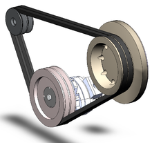
V belts


V belts (also style V-belts, vee belts, or, less commonly, wedge rope) solved the slippage and alignment problem. It is now the basic belt for power transmission. They provide the best combination of traction, speed of movement, load of the bearings, and long service life. They are generally endless, and their general cross-section shape is roughly trapezoidal (hence the name "V"). The "V" shape of the belt tracks in a mating groove in the pulley (or sheave), with the result that the belt cannot slip off. The belt also tends to wedge into the groove as the load increases—the greater the load, the greater the wedging action—improving torque transmission and making the V-belt an effective solution, needing less width and tension than flat belts. V-belts trump flat belts with their small center distances and high reduction ratios. The preferred center distance is larger than the largest pulley diameter, but less than three times the sum of both pulleys. Optimal speed range is 1,000–7,000 ft/min (300–2,130 m/min). V-belts need larger pulleys for their thicker cross-section than flat belts.
For high-power requirements, two or more V-belts can be joined side-by-side in an arrangement called a multi-V, running on matching multi-groove sheaves. This is known as a multiple-V-belt drive (or sometimes a "classical V-belt drive").
V-belts may be homogeneously rubber or polymer throughout, or there may be fibers embedded in the rubber or polymer for strength and reinforcement. The fibers may be of textile materials such as cotton, polyamide (such as Nylon) or polyester or, for greatest strength, of steel or aramid (such as Technora, Twaron or Kevlar).
When an endless belt does not fit the need, jointed and link V-belts may be employed. Most models offer the same power and speed ratings as equivalently-sized endless belts and do not require special pulleys to operate. A link v-belt is a number of polyurethane/polyester composite links held together, either by themselves, such as Fenner Drives' PowerTwist, or Nu-T-Link (with metal studs). These provide easy installation and superior environmental resistance compared to rubber belts and are length-adjustable by disassembling and removing links when needed.
Multi-groove belts
A multi-groove, V-Ribbed, or polygroove belt is made up of usually between 3 and 24 "V" shaped sections alongside each other. This gives a thinner belt for the same drive surface, thus it is more flexible, although often wider. The added flexibility offers an improved efficiency, as less energy is wasted in the internal friction of continually bending the belt. In practice this gain of efficiency causes a reduced heating effect on the belt, and a cooler-running belt lasts longer in service. Belts are commercially available in several sizes, with usually a 'P' (sometimes omitted) and a single letter identifying the pitch between grooves. The 'PK' section with a pitch of 3.56 mm is commonly used for automotive applications.
A further advantage of the polygroove belt that makes them popular is that they can run over pulleys on the ungrooved back of the belt. Though this is sometimes done with V-belts with a single idler pulley for tensioning, a polygroove belt may be wrapped around a pulley on its back tightly enough to change its direction, or even to provide a light driving force.
Any V-belt's ability to drive pulleys depends on wrapping the belt around a sufficient angle of the pulley to provide grip. Where a single-V-belt is limited to a simple convex shape, it can adequately wrap at most three or possibly four pulleys, so can drive at most three accessories. Where more must be driven, such as for modern cars with power steering and air conditioning, multiple belts are required. As the polygroove belt can be bent into concave paths by external idlers, it can wrap any number of driven pulleys, limited only by the power capacity of the belt.
This ability to bend the belt at the designer's whim allows it to take a complex or "serpentine" path. This can assist the design of a compact engine layout, where the accessories are mounted more closely to the engine block and without the need to provide movable tensioning adjustments. The entire belt may be tensioned by a single idler pulley.
Ribbed belt
A ribbed belt is a power transmission belt featuring lengthwise grooves. It operates from contact between the ribs of the belt and the grooves in the pulley. Its single-piece structure is reported to offer an even distribution of tension across the width of the pulley where the belt is in contact, a power range up to 600 kW, a high speed ratio, serpentine drives (possibility to drive off the back of the belt), long life, stability and homogeneity of the drive tension, and reduced vibration. The ribbed belt may be fitted on various applications: compressors, fitness bikes, agricultural machinery, food mixers, washing machines, lawn mowers, etc.
Film belts
Though often grouped with flat belts, they are actually a different kind. They consist of a very thin belt (0.5–15 millimeters or 100–4000 micrometres) strip of plastic and occasionally rubber. They are generally intended for low-power (less than 10 watts), high-speed uses, allowing high efficiency (up to 98%) and long life. These are seen in business machines, printers, tape recorders, and other light-duty operations.
Timing belts


Timing belts (also known as toothed, notch, cog, or synchronous belts) are a positive transfer belt and can track relative movement. These belts have teeth that fit into a matching toothed pulley. When correctly tensioned, they have no slippage, run at constant speed, and are often used to transfer direct motion for indexing or timing purposes (hence their name). They are often used instead of chains or gears, so there is less noise and a lubrication bath is not necessary. Camshafts of automobiles, miniature timing systems, and stepper motors often utilize these belts. Timing belts need the least tension of all belts and are among the most efficient. They can bear up to 200 hp (150 kW) at speeds of 16,000 ft/min (4,900 m/min).
Timing belts with a helical offset tooth design are available. The helical offset tooth design forms a chevron pattern and causes the teeth to engage progressively. The chevron pattern design is self-aligning and does not make the noise that some timing belts make at certain speeds, and is more efficient at transferring power (up to 98%).
Disadvantages include a relatively high purchase cost, the need for specially fabricated toothed pulleys, less protection from overloading, jamming, and vibration due to their continuous tension cords, the lack of clutch action (only possible with friction-drive belts), and the fixed lengths, which do not allow length adjustment (unlike link V-belts or chains).
Specialty belts
Belts normally transmit power on the tension side of the loop. However, designs for continuously variable transmissions exist that use belts that are a series of solid metal blocks, linked together as in a chain, transmitting power on the compression side of the loop.
Rolling roads
Belts used for rolling roads for wind tunnels can be capable of 250 km/h (160 mph).[16]
Standards for use
The open belt drive has parallel shafts rotating in the same direction, whereas the cross-belt drive also bears parallel shafts but rotate in opposite direction. The former is far more common, and the latter not appropriate for timing and standard V-belts unless there is a twist between each pulley so that the pulleys only contact the same belt surface. Nonparallel shafts can be connected if the belt's center line is aligned with the center plane of the pulley. Industrial belts are usually reinforced rubber but sometimes leather types. Non-leather, non-reinforced belts can only be used in light applications.
The pitch line is the line between the inner and outer surfaces that is neither subject to tension (like the outer surface) nor compression (like the inner). It is midway through the surfaces in film and flat belts and dependent on cross-sectional shape and size in timing and V-belts. Calculating pitch diameter is an engineering task and is beyond the scope of this article. The angular speed is inversely proportional to size, so the larger the one wheel, the less angular velocity, and vice versa. Actual pulley speeds tend to be 0.5–1% less than generally calculated because of belt slip and stretch. In timing belts, the inverse ratio teeth of the belt contributes to the exact measurement. The speed of the belt is:
Speed = Circumference based on pitch diameter × angular speed in rpm
Selection criteria
Belt drives are built under the following required conditions: speeds of and power transmitted between drive and driven unit; suitable distance between shafts; and appropriate operating conditions. The equation for power is
- power [kW] = (torque [N·m]) × (rotational speed [rev/min]) × (2π radians) / (60 s × 1000 W).
Factors of power adjustment include speed ratio; shaft distance (long or short); type of drive unit (electric motor, internal combustion engine); service environment (oily, wet, dusty); driven unit loads (jerky, shock, reversed); and pulley-belt arrangement (open, crossed, turned). These are found in engineering handbooks and manufacturer's literature. When corrected, the power is compared to rated powers of the standard belt cross-sections at particular belt speeds to find a number of arrays that perform best. Now the pulley diameters are chosen. It is generally either large diameters or large cross-section that are chosen, since, as stated earlier, larger belts transmit this same power at low belt speeds as smaller belts do at high speeds. To keep the driving part at its smallest, minimal-diameter pulleys are desired. Minimum pulley diameters are limited by the elongation of the belt's outer fibers as the belt wraps around the pulleys. Small pulleys increase this elongation, greatly reducing belt life. Minimal pulley diameters are often listed with each cross-section and speed, or listed separately by belt cross-section. After the cheapest diameters and belt section are chosen, the belt length is computed. If endless belts are used, the desired shaft spacing may need adjusting to accommodate standard-length belts. It is often more economical to use two or more juxtaposed V-belts, rather than one larger belt.
In large speed ratios or small central distances, the angle of contact between the belt and pulley may be less than 180°. If this is the case, the drive power must be further increased, according to manufacturer's tables, and the selection process repeated. This is because power capacities are based on the standard of a 180° contact angle. Smaller contact angles mean less area for the belt to obtain traction, and thus the belt carries less power.
Belt friction
Belt drives depend on friction to operate, but excessive friction wastes energy and rapidly wears the belt. Factors that affect belt friction include belt tension, contact angle, and the materials used to make the belt and pulleys.
Belt tension
Power transmission is a function of belt tension. However, also increasing with tension is stress (load) on the belt and bearings. The ideal belt is that of the lowest tension that does not slip in high loads. Belt tensions should also be adjusted to belt type, size, speed, and pulley diameters. Belt tension is determined by measuring the force to deflect the belt a given distance per inch of pulley. Timing belts need only adequate tension to keep the belt in contact with the pulley.
Belt wear
Fatigue, more so than abrasion, is the culprit for most belt problems. This wear is caused by stress from rolling around the pulleys. High belt tension; excessive slippage; adverse environmental conditions; and belt overloads caused by shock, vibration, or belt slapping all contribute to belt fatigue.
Belt vibration
Vibration signatures are widely used for studying belt drive malfunctions. Some of the common malfunctions or faults include the effects of belt tension, speed, sheave eccentricity and misalignment conditions.The effect of sheave Eccentricity on vibration signatures of the belt drive is quite significant. Although, vibration magnitude is not necessarily increased by this it will create strong amplitude modulation. When the top section of a belt is in resonance, the vibrations of the machine is increased. However, an increase in the machine vibration is not significant when only the bottom section of the belt is in resonance. The vibration spectrum has the tendency to move to higher frequencies as the tension force of the belt is increased.
Belt dressing
Belt slippage can be addressed in several ways. Belt replacement is an obvious solution, and eventually the mandatory one (because no belt lasts forever). Often, though, before the replacement option is executed, retensioning (via pulley centerline adjustment) or dressing (with any of various coatings) may be successful to extend the belt's lifespan and postpone replacement. Belt dressings are typically liquids that are poured, brushed, dripped, or sprayed onto the belt surface and allowed to spread around; they are meant to recondition the belt's driving surfaces and increase friction between the belt and the pulleys. Some belt dressings are dark and sticky, resembling tar or syrup; some are thin and clear, resembling mineral spirits. Some are sold to the public in aerosol cans at auto parts stores; others are sold in drums only to industrial users.
Specifications
To fully specify a belt, the material, length, and cross-section size and shape are required. Timing belts, in addition, require that the size of the teeth be given. The length of the belt is the sum of the central length of the system on both sides, half the circumference of both pulleys, an d the square of the sum (if crossed) or the difference (if open) of the radii. Thus, when dividing by the central distance, it can be visualized as the central distance times the height that gives the same squared value of the radius difference on, of course, both sides. When adding to the length of either side, the length of the belt increases, in a similar manner to the Pythagorean theorem. One important concept to remember is that as D1 gets closer to D2 there is less of a distance (and therefore less addition of length) until its approaches zero.
On the other hand, in a crossed belt drive the sum rather than the difference of radii is the basis for computation for length. So the wider the small drive increases, the belt length is higher.
V-belt profiles

Metric v-belt profiles:
| Classic profile | Width | Height | Angle* | Remarks |
|---|---|---|---|---|
| Z | 10mm | - | - | |
| A | 13mm | 15mm | 40° | 12.7mm = 0.5 inch width, 38° angle if inches |
| B | 17mm | 11mm | 40° | 16.5mm = 21/32 inch width, 38° angle if inches |
| C | 22mm | 14mm | 40° | 22.2mm = 7/8 inch width, 38° angle if inches |
| D | 32mm | 19mm | 40° | 31.75mm = 1.25 inch width, 38° angle if inches |
| E | 38mm | 25mm | 40° | 38.1mm = 1.5 inch width, 38° angle if inches |
| Narrow-profile | Width | Height | Angle* | Remarks |
| SPZ | 10mm | 8mm | 34° | |
| SPA | 13mm | - | - | |
| SPB | 17mm | - | - | |
| SPC | 22mm | - | - | |
| High-Performance Narrow-profile | Width | Height | Angle* | Remarks |
| XPZ | 10mm | - | - | |
| XPA | 13mm | - | - | |
| XPB | 17mm | - | - | |
| XPC | 22mm | - | - |
- Common pulley design is to have a higher angle of the first part of the opening, above the so called "pitch line".
E.g. the pitch line for SPZ could be 8.5mm from the bottom of the "V". In other words 0-8.5mm is 34° and 38° from 8.5 and above
Timing Belt
A timing belt, timing chain or cambelt is a part of an internal combustion engine that synchronizes the rotation of the crankshaft and the camshaft(s) so that the engine's valves open and close at the proper times during each cylinder's intake and exhaust strokes. In an interference engine the timing belt or chain is also critical to preventing the piston from striking the valves. A timing belt is usually a toothed belt -- a drive belt with teeth on the inside surface. A timing chain is a roller chain.

Many modern production automobile engines use a timing belt[i] to synchronize crankshaft and camshaft rotation; some engines, particularly cam in block designs, used gears to drive the camshaft, but this was rare for OHC designs. The use of a timing belt or chain instead of gear drive enables engine designers to place the camshaft(s) further from the crankshaft, and in engines with multiple camshafts a timing belt or chain also enables the camshafts to be placed further from each other. Timing chains were common on production automobiles through the 1970s and 1980s, when timing belts became the norm, but timing chains have seen a resurgence in recent years. Timing chains are generally more durable than timing belts – though neither is as durable as gear drive – however, timing belts are lighter, less expensive, and operate more quietly.
 Timing Belt
Engine applications

In the internal combustion engine application the timing belt or chain connects the crankshaft to the camshaft(s), which in turn control the opening and closing of the engine's valves. A four-stroke engine requires that the valves open and close once every other revolution of the crankshaft. The timing belt does this. It has teeth to turn the camshaft(s) synchronised with the crankshaft, and is specifically designed for a particular engine. In some engine designs the timing belt may also be used to drive other engine components such as the water pump and oil pump.
Types
Gear or chain systems are also used to connect the crankshaft to the camshaft at the correct timing. However, gears and shafts constrain the relative location of the crankshaft and camshafts. Even where the crankshaft and camshaft(s) are very close together, as in pushrod engines, most engine designers use a short chain drive rather than a direct gear drive. This is because gear drives suffer from frequent torque reversal as the cam profiles "kick back" against the drive from the crank, leading to excessive noise and wear. Fibre or nylon covered gears, with more resilience, are often used instead of steel gears where direct drive is used. Commercial engines and aircraft engines use steel gears only, as a fibre or nylon coated gear can fail suddenly and without warning.[1]
A belt or chain allows much more flexibility in the relative locations of the crankshaft and camshafts.
While chains and gears may be more durable, rubber composite belts are quieter in their operation (in most modern engines the noise difference is negligible), are less expensive and more efficient, by dint of being lighter, when compared with a gear or chain system. Also, timing belts do not require lubrication, which is essential with a timing chain or gears. A timing belt is a specific application of a synchronous belt used to transmit rotational power synchronously.
Timing belts are typically covered by metal or polymer timing belt covers which require removal for inspection or replacement. Engine manufacturers recommend replacement at specific intervals. The manufacturer may also recommend the replacement of other parts, such as the water pump, when the timing belt is replaced because the additional cost to replace the water pump is negligible compared to the cost of accessing the timing belt. In an interference engine, or one whose valves extend into the path of the piston, failure of the timing belt (or timing chain) invariably results in costly and, in some cases, irreparable engine damage, as some valves will be held open when they should not be and thus will be struck by the pistons.
Indicators that the timing chain may need to be replaced include a rattling noise from the front of the engine.
Failure[

Timing belts must be replaced at the manufacturer's recommended distance and/or time periods. Failure to replace the belt can result in complete breakdown or catastrophic engine failure, especially in interference engines.[4]The owner's manual maintenance schedule is the source of timing belt replacement intervals, typically every 30,000 to 50,000 miles (50,000 to 80,000 km).[5] It is common to replace the timing belt tensioner at the same time as the belt is replaced.
The usual failure modes of timing belts are either stripped teeth (which leaves a smooth section of belt where the drive cog will slip) or delamination and unraveling of the fiber cores. Breakage of the belt, because of the nature of the high tensile fibers, is uncommon. Often overlooked, debris and dirt that mix with oil and grease can slowly wear at the belt and materials advancing the wear process, causing premature belt failure.[7] Correct belt tension is critical - too loose and the belt will whip, too tight and it will whine and put excess strain on the bearings of the cogs. In either case belt life will be drastically shortened. Aside from the belt itself, also common is a failure of the tensioner, and/or the various gear and idler bearings, causing the belt to derail.
When an automotive timing belt is replaced, care must be taken to ensure that the valve and piston movements are correctly synchronized. Failure to synchronize correctly can lead to problems with valve timing, and this in turn, in extremes, can cause collision between valves and pistons in interference engines. This is not a problem unique to timing belts since the same issue exists with all other cam/crank timing methods such as gears or chains.
Construction and design
A timing belt is typically rubber with high-tensile fibres (e.g. fiberglass or Twaron/Kevlar) running the length of the belt as tension members.[8] The belt itself is constructed in sturdy materials such as molded polyurethane, neoprene or welded urethane with various standard, non-standard or metric pitches.[9] The distance between the centers of two adjacent teeth on the timing belt is referred to as the pitch.
Rubber degrades with higher temperatures, and with contact with motor oil. Thus the life expectancy of a timing belt is lowered in hot or leaky engines. Newer or more expensive belts are made of temperature resistant materials such as "highly saturated nitrile" (HSN).[citation needed] The life of the reinforcing cords is also greatly affected by water and antifreeze. This means that special precautions must be taken for off road applications to allow water to drain away or be sealed from contact with the belt.
Older belts have trapezoid shaped teeth leading to high rates of tooth wear. Newer manufacturing techniques allow for curved teeth that are quieter and last longer.
Aftermarket timing belts may be used to alter engine performance. OEM timing belts may stretch at high rpm, retarding the cam and therefore the ignition.[11] Stronger, aftermarket belts, will not stretch and the timing is preserved. In terms of engine design, "shortening the width of the timing belt reduce[s] weight and friction"
Continuously variable transmission
A continuously variable transmission (CVT), also known as a shiftless transmission, single-speed transmission, stepless transmission, pulley transmission, or, in case of motorcycles, a 'twist-and-go', is an automatic transmission that can change seamlessly through a continuous range of effective gear ratios. This contrasts with other mechanical transmissions that offer a fixed number of gear ratios. The flexibility of a CVT with suitable control may allow the input shaft to maintain a constant angular velocity even as the output speed varies.
A belt-driven design offers approximately 88% efficiency,[1] which, while lower than that of a manual transmission, can be offset by lower production cost and by enabling the engine to run at its most efficient speed for a range of output speeds. When power is more important than economy, the ratio of the CVT can be changed to allow the engine to turn at the RPM at which it produces greatest power. This is typically higher than the RPM that achieves peak efficiency. In low-mass low-torque applications (such as motor scooters) a belt-driven CVT also offers ease of use and mechanical simplicity.
A CVT does not strictly require the presence of a clutch. Nevertheless, in some vehicles (e.g. motorcycles), a centrifugal clutch is added[2] to facilitate a "neutral" stance, which is useful when idling or manually reversing
Uses


Motorized vehicles
Simple rubber belt (non-stretching fixed circumference manufactured using various highly durable and flexible materials) CVTs are commonly used in small motorized vehicles, where their mechanical simplicity and ease of use outweigh their comparative inefficiency. Nearly all snowmobiles, utility vehicles, golf carts and motor scooters use CVTs, typically the rubber belt or variable pulley variety.
CVTs were banned from Formula 1 in 1994 because of concerns that the best-funded teams would dominate if they managed to create a viable F1 CVT.
More recently,, CVT systems have been developed for go-karts and have proven to increase performance and engine life expectancy. The Tomcar range of off-road vehicles also utilizes the CVT system.
Some vehicles that offer CVT are the Chrysler Pacifica hybrid, the Ford C-MAX hybrid, the Mitsubishi Lancer, the Dodge Caliber, the Toyota Corolla, the Scion iQ, the Honda Insight, Fit, CR-Z hybrid, CR-V, Capa, Honda Civic, Honda Accord, the Nissan Tiida/Versa (SL, SV, and Note S Plus or higher models), Cube, Juke, Sentra, Altima, Maxima, 2013 1.2 Note, Rogue, X-Trail, Murano, Pathfinder, Sunny and the non-Mexican Micra, the Jeep Patriot and Compass, the Suzuki SX4 S-Cross, and the Subaru Forester, Impreza, Legacy, Outback and Crosstrek, Suzuki Kizashi, Toyota Allion 2009 onwards, Toyota Premio 2009 onwards, Toyota Avalon, Toyota Mark X, etc.
CVTs should be distinguished from power-sharing transmissions (PSTs), as used in newer hybrid cars, such as the Toyota Prius, Highlander and Camry, the Nissan Altima, and newer-model Ford Escape Hybrid SUVs. CVT technology uses only one input from a prime mover and delivers variable output speeds and torque, whereas PST technology uses two prime mover inputs and varies the ratio of their contributions to output speed and power. These transmissions are fundamentally different.
Farm equipment, namely harvester combines, used variable belt drives as early as the 1950s, as well. Many small tractors and self-propelled mowers for home and garden also use simple rubber belt CVT. Hydrostatic systems are more common on the larger units—the walk-behind self-propelled mowers are of the slipping belt variety.
Ratcheting CVT converting rotary motion to oscillating motion and back to rotary motion using roller clutches are well adapted to reciprocating engines when the oscillating movement is synchronized with that of the pistons. This solution could have a bright future because such ratcheting CVT are also IVT (providing the clutch function), and have a very high energy efficiency. They could help automakers comply with the future emission standards, while also improving the reciprocating engines performance.
Downsizing electric engines
Instead of being dimensioned according to the maximum torque (eg that required for starting, or in case of momentary mechanical overload), the motors using this type of CVT may be dimensioned by matching the maximum power with the maximum desired speed (that of a vehicle by example). Such CVT is used only at startup or in case of mechanical overload, and may be disconnected most of the time, the engine transfering the torque directly to the output. New concepts adapting the transmission ratio to the resistant torque and centrifugal clutch may be used to make these changes automatic.
Bicycles
A ratchet CVT has been proposed for bicycles The crankset causes a lever to swing, which in turn causes the reciprocating movement of a double rack that rotates the wheel as it moves backward and as it moves toward the wheel.
Medium and high power transfers
Hydrostatic CVTs are common in small to medium-sized agricultural and earthmoving equipment. As the engines in these machines are typically run at constant power settings to provide hydraulic power or to power machinery, losses in mechanical efficiency are offset by enhanced operational efficiency, such as reduced forward-reverse shuttle times in earthmoving operations. Transmission output is varied to control both travel speed and direction. This is particularly beneficial in equipment designed to pivot or skid steer through differential power application as the required differential steering action can easily be supplied by independent CVTs, allowing steering to be accomplished without braking losses or loss of tractive effort and allowing the machine to pivot in place. In mowing or harvesting operations a CVT allows the forward speed of the tractor or combine harvester to be adjusted independently of the engine speed. This allows the operator to slow or accelerate as needed to accommodate variations in thickness of the crop.
Power generating systems
CVTs have been used in aircraft electrical power generating systems since the 1950s and in Sports Car Club of America (SCCA) Formula 500 race cars since the early 1970s.
Some drill presses and milling machines contain a pulley-based CVT system where the output shaft has a pair of manually adjustable conical pulley halves through which a wide drive belt from the motor loops. The pulley on the motor, however, is usually fixed in diameter, or may have a series of given-diameter steps to allow a selection of speed ranges. A handwheel on the drill press, marked with a scale corresponding to the desired machine speed, is mounted to a reduction gearing system for the operator to precisely control the width of the gap between the pulley halves. This gap width thus adjusts the gearing ratio between the motor's fixed pulley and the output shaft's variable pulley, changing speed of the chuck. A tensioner pulley is implemented in the belt transmission to take up or release the slack in the belt as the speed is altered. In most cases, the speed must be changed with the motor running.
Doubly-fed induction generators are usually coupled with multi-stage gearboxes to increase the rotational speed. These gearboxes might be replaced by fully CVT in the future, but only fully geared one because they are the only ones providing a sufficient mechanical efficiency
A CVT and flywheel may be inserted between an energy source (eg a wind turbine) and the electricity generator. When the energy source is sufficient, the generator is connected directly to the CVT which serves to regulate its speed of rotation. When it is too low, the generator is disconnected and the energy stored in the flywheel. It is only when the speed of the flywheel is sufficient that the kinetik energy is converted into electricity, intermittently, but always at the optimal speed of the generator.
Winches and hoists
It's also an application of CVTs, especially for those adapting the transmission ratio to the resistant torque.
Types


Variable-diameter pulley (VDP) or Reeves drive
In this most common CVT system,[6] there are two V-belt pulleys that are split perpendicular to their axes of rotation, with a V-belt running between them. The gear ratio is changed by moving the two sheaves of one pulley closer together and the two sheaves of the other pulley farther apart. The V-shaped cross section of the belt causes it to ride higher on one pulley and lower on the other. This changes the effective diameters of both pulleys, which changes the overall gear ratio. As the distance between the pulleys and the length of the belt does not change, both pulleys must be adjusted (one bigger, the other smaller) simultaneously in order to maintain the proper amount of tension on the belt. Simple CVTs combining a centrifugal drive pulley with a spring loaded driven pulley often use belt tension to effect the conforming adjustments in the driven pulley. The V-belt needs to be very stiff in the pulley's axial direction in order to make only short radial movements while sliding in and out of the pulleys. The Chinese gy6-type scooter uses this type of CVT drive system.
Steel reinforced v-belts are sufficient for low-mass low-torque applications like utility vehicles and snowmobiles but higher mass and torque applications such as automobiles require a chain. Each element of the chain must have conical sides that fit the pulley when the belt is running on the outermost radius. As the chain moves into the pulleys the contact area gets smaller. As the contact area is proportional to the number of elements, chain belts require lots of very small elements. The shape of the elements is governed by the static of a column. The pulley-radial thickness of the belt is a compromise between maximum gear ratio and torque. For the same reason the axis between the pulleys is as thin as possible. In a chain-based CVT a film of lubricant is applied to the pulleys. It needs to be thick enough so that the pulley and the chain never touch and it must be thin in order not to waste power when each element dives into the lubrication film. Additionally, the chain elements stabilize about 12 steel bands. Each band is thin enough so that it bends easily. If bending, it has a perfect conical surface on its side. In the stack of bands each band corresponds to a slightly different gear ratio, and thus they slide over each other and need oil between them. Also the outer bands slide through the stabilizing chain, while the center band can be used as the chain linkage.[note 1]

Push-Belt
While some CVTs transmit torque only through the tension of the belt or chain, a push-belt CVT transmits torque both through "pulling" belt ring tension and also "pushing" link element compression.
Toroidal or roller-based (Extroid)
Toroidal CVTs are made up of discs and rollers that transmit power between the discs. The discs can be pictured as two almost conical parts, point to point, with the sides dished such that the two parts could fill the central hole of a torus. One disc is the input, and the other is the output. Between the discs are rollers which vary the ratio and which transfer power from one side to the other. When the roller's axis is perpendicular to the axis of the near-conical parts, it contacts the near-conical parts at same-diameter locations and thus gives a 1:1 gear ratio. The roller can be moved along the axis of the near-conical parts, changing angle as needed to maintain contact. This will cause the roller to contact the near-conical parts at varying and distinct diameters, giving a gear ratio of something other than 1:1. Systems may be partial or full toroidal. Full toroidal systems are the most efficient design while partial toroidals may still require a torque converter, and hence lose efficiency.
Some toroidal systems like the torotrak, are also infinitely variable, and the direction of thrust can be reversed within the CVT.
Diagrams:
Examples:
- Nissan Extroid CVT (pdf on Nissan-Global site)
Magnetic or mCVT
A magnetic continuous variable transmission system was developed at the University of Sheffield in 2006 and later commercialized.[11] mCVT is a variable magnetic transmission which gives an electrically controllable gear ratio. It can act as a power split device and can match a fixed input speed from a prime-mover to a variable load by importing/exporting electrical power through a variator path. The mCVT is of particular interest as a highly efficient power-split device for blended parallel hybrid vehicles, but also has potential applications in renewable energy, marine propulsion and industrial drive sectors.
Infinitely variable transmission (IVT)
A subset of CVT designs are called infinitely variable transmissions (IVT or IVTs), in which the range of ratios of output shaft speed to input shaft speed includes a zero ratio that can be continuously approached from a defined "higher" ratio. A zero output speed (low gear) with a finite input speed implies an infinite input-to-output speed ratio, which can be continuously approached from a given finite input value with an IVT. Low gears are a reference to low ratios of output speed to input speed. This low ratio is taken to the extreme with IVTs, resulting in a "neutral", or non-driving "low" gear limit, in which the output speed is zero. Unlike neutral in a normal automotive transmission, IVT output rotation may be prevented because the back-driving (reverse IVT operation) ratio may be infinite, resulting in impossibly high backdriving torque; in a ratcheting IVT, however, the output may freely rotate in the forward direction.
Friction
In the early decades of the 20th century, several tractors and small locomotives were built with friction-disk transmissions with an output disk rolling on the face of the input disk. For disks of identical diameter, the effective gear ratio could be varied from 1:1 when the point of contact was at the perimeter of the input disk, to infinity when the point of contact was at the center, to -1:1 when the point of contact was at the opposite extreme. The transmission on early Plymouth locomotives worked this way, while on tractors using friction disks, the range of reverse speeds was typically limited.
Epicyclic gearing
Many IVTs result from the combination of a CVT with a planetary gear system which enforces an IVT output shaft rotation speed which is equal to the difference between two other speeds within the IVT. This IVT configuration uses its CVT as a continuously variable regulator (CVR) of the rotation speed of any one of the three rotators of the planetary gear system (PGS). If two of the PGS rotator speeds are the input and output of the CVR, there is a setting of the CVR that results in the IVT output speed of zero. The maximum output/input ratio can be chosen from infinite practical possibilities through selection of additional input or output gear, pulley or sprocket sizes without affecting the zero output or the continuity of the whole system. The IVT is always engaged, even during its zero output adjustment.
IVTs can in some implementations offer better efficiency in the preferred range of operation when compared to other CVTs because most of the power flows through the planetary gear system and not the controlling CVR. Torque transmission capability can also be increased. Staging power splits is also possible for further increase in efficiency, torque transmission capability and better maintenance of efficiency over a wide gear ratio range.
Examples
Hydristor
An example of a true IVT is the Hydristor because the front unit connected to the engine can displace from zero to 27 cubic inches (440 cm3) per revolution forward and zero to −10 cubic inches (−160 cm3) per revolution reverse. The rear unit is capable of zero to 75 cubic inches (1,230 cm3) per revolution. However, whether this design enters production remains to be seen.fact Another example of a true IVT that has been put into recent production and which continues under commercial development[ is that of Torotrak.
Guigan

A French inventor, Franck Guigan, filed patent applications in 2017 for a method based on variable diameter gears (PCT/FR2017000174). This new method eliminates any oscillatory movement that could cause vibration. It is a true IVT as the variable diameter of the crown allows the transmission ratio to vary from any positive value to any negative value passing through a ZERO position. It also works as a regenerative braking system, which can be used as a kinetic energy recovery system. It also allows to combine two engines, for example a combustion engine and an electric one.
Franck Guigan filed in 2018 patent applications for a method based on oscillating racks combined with freewheels, which gave rise to many different transmissions.

This transmission is also a true IVT as the transmission ratio can be ZERO, which means that it allows not to use any clutch. Although there is an oscillatory movement, some of these transmissions are absolutely homokinetic, which means the rotation of the output shaft is at all times exactly proportional to the one of the input shaft. The MultiRack transmission shown on the right will work most of the time in "direct drive" mode, the output shaft being directly connected to the input and the racks remaining stationary, and it is only in case of mechanical overload, that the CVT will come into play. A new feature is that the transmission ratio may be permanently adapted to the resistive torque. This is what allows to use downsized engines (e.g. electric), that are lighter, less bulky and more economical to build and to use. Not only does this device guarantee the constant supply of sufficient torque, but it also protects the engine.
In both cases, the transmission ratio can be chosen manually or computer-determined.
Ratcheting
The ratcheting CVT is a transmission that relies on static friction and is based on a set of elements that successively become engaged and then disengaged between the driving system and the driven system, often using oscillating or indexing motion in conjunction with one-way clutches or ratchets that rectify and sum only "forward" motion. The transmission ratio is adjusted by changing linkage geometry within the oscillating elements, so that the summed maximum linkage speed is adjusted, even when the average linkage speed remains constant. Power is transferred from input to output only when the clutch or ratchet is engaged, and therefore when it is locked into a static friction mode where the driving & driven rotating surfaces momentarily rotate together without slippage.
One type of ratcheting CVT that is not dependent on friction uses a scotch yoke mechanism to convert rotation to linear oscillation. The magnitude of oscillation, sometimes called "stroke", depends on the distance of the crank pin in the scotch yoke mechanism from the axis of rotation. The stroke is altered by altering the distance of the crank pin from the axis of rotation. This linear oscillation is converted back to rocking motion using a rack and pinion. This rocking motion is rectified to rotation using either computer controlled clutch, sprag clutch or one-way bearing. The main advantage of this type of CVT is that it is not dependent on friction to transmit power. One drawback here is that the input to output ratio is sinusoidal and not constant. However, patented designs exist to overcome this drawback by altering the instantaneous rotational speed of the scotch yoke mechanism using non-circular gears. An example of a non-friction-dependent ratcheting CVT having a constant input to output ratio, is patent protected under U.S. Patent 9,970,520B2.
These CVTs can transfer substantial torque, because their static friction actually increases relative to torque throughput, so slippage is impossible in properly designed systems. Efficiency is generally high, because most of the dynamic friction is caused by very slight transitional clutch speed changes. The drawback to ratcheting CVTs is vibration caused by the successive transition in speed required to accelerate the element, which must supplant the previously operating and decelerating, power transmitting element.
Ratcheting CVTs are distinguished from VDPs and roller-based CVTs by being static friction-based devices, as opposed to being dynamic friction-based devices that waste significant energy through slippage of twisting surfaces. An example of a ratcheting CVT is one prototyped as a bicycle transmission protected under U.S. Patent 5,516,132 in which strong pedalling torque causes this mechanism to react against the spring, moving the ring gear/chainwheel assembly toward a concentric, lower gear position. When the pedaling torque relaxes to lower levels, the transmission self-adjusts toward higher gears, accompanied by an increase in transmission vibration.
The ratcheting IVT dates back to before the 1930s; the original design converts rotary motion to oscillating motion and back to rotary motion using roller clutches.[17] The stroke of the intermediate oscillations is adjustable, varying the output speed of the shaft. The fundamental limitation is that when the torque transfers between the separate oscillatory paths the change in deflection causes high vibration at higher torques. The original design is still manufactured today, and an example and animation of this IVT can be found here.[18] Paul B. Pires created a more compact (radially symmetric) variation that employs a ratchet mechanism instead of roller clutches, so it does not have to rely on friction to drive the output. An article and sketch of this variation can be found here [19]
Hydrostatic


Hydrostatic transmissions use a variable displacement pump and a hydraulic motor. All power is transmitted by hydraulic fluid. These types can generally transmit more torque, but can be sensitive to contamination. Some designs are also very expensive. However, they have the advantage that the hydraulic motor can be mounted directly to the wheel hub, allowing a more flexible suspension system and eliminating efficiency losses from friction in the drive shaft and differential components. This type of transmission is relatively easy to use because all forward and reverse speeds can be accessed using a single lever.
An integrated hydrostatic transaxle (IHT) uses a single housing for both hydraulic elements and gear-reducing elements. This type of transmission has been effectively applied to a variety of inexpensive and expensive versions of ridden lawn mowers and garden tractors.
One class of riding lawn mower that has recently gained in popularity with consumers is zero turning radius mowers. These mowers have traditionally been powered with wheel hub mounted hydraulic motors driven by continuously variable pumps, but this design is relatively expensive.
Some heavy equipment may also be propelled by a hydrostatic transmission; e.g. agricultural machinery including foragers, combines, and some tractors. A variety of heavy earth-moving equipment, e.g. compact and small wheel loaders, track type loaders and crawler tractors, skid-steered loaders and asphalt compactors use hydrostatic transmission. Hydrostatic CVTs are usually not used for extended duration high torque applications because of the heat that is generated by the flowing oil, although there are a variety of oil cooler designs to help counter this problem.
The Honda DN-01 motorcycle is the first road-going consumer vehicle with hydrostatic drive that employs a variable displacement axial piston pump with a variable-angle swashplate.
AGCO Corporation has employed a hydrostatic CVT transmission in agricultural equipment. The transmission splits power between hydrostatic and mechanical transfer to the output shaft via a planetary gear in the forward direction of travel. In reverse the power transfer is fully hydrostatic.
Naudic incremental (iCVT)
This is a chain-driven system. Although an iCVT works, it has the following weakness:
High frictional losses
The variator pulley of an iCVT is choked using two small choking pulleys. Here one choking pulley is positioned on the tense side of the chain of the iCVT. Hence there is a considerable load on that choking pulley, the magnitude of which is proportional to the tension in its chain. Each choking pulley is pulled up by two chain segments, one chain segment to the left and one to the right of the choking pulley; here if the two chain segments are parallel to each other, then the load on the choking pulley is twice the tension in the chain. But since the two chain segments are most likely not parallel to each other during operations of an iCVT, it is estimated that the load on a choking pulley is between 1 and 1.8 times of the tension of its chain.
Also, a choking pulley is very small so that its moment arm is very small. A larger moment arm reduces the force needed to rotate a pulley. For example, using a long wrench, which has a large moment arm, to open a nut requires less force than using a short wrench, which has a small moment arm. Assuming that the diameter of a choking pulley is twice the diameter of its shaft, which is a generous estimate, then the frictional resistance force at the outer diameter of a choking pulley is half the frictional resistance force at the shaft of a choking pulley.
Shock and durability
The transmission ratio of an iCVT has to be changed one increment within less than one full rotation of its variator pulley. This means that the transmission diameter of the variator pulley, made generally from rubber, has to be changed from a diameter that has a circumferential length that is equal to an integer number of teeth to another diameter that has a circumferential length that is equal to an integer number of teeth; such as changing the transmission diameter of the variator pulley from a diameter that has a circumferential length of 7 teeth to a diameter that has a circumferential length of 8 teeth for example. This is because if the transmission diameter of the variator pulley does not have a circumferential length that is equal to an integer number of teeth, such as a circumferential length of 71⁄2 teeth for example, improper engagement between the teeth of the variator pulley and its chain will occur. For example, imagine having a bicycle pulley with 71⁄2 teeth; here improper engagement between the bicycle pulley and its chain will occur when the tooth behind the 1⁄2 tooth space is about to engage with its chain, since it is positioned a distance of 1⁄2 tooth too late relative to its chain.
Regarding the previous paragraph, the chain of an iCVT forms an open loop on its variator pulley that partially covers its variator pulley such that an open section, which is not covered by the chain, exist. This is similar to a sprocket of a bicycle where there is a section of the sprocket that is covered by its chain, and a section of the sprocket that is not covered by its chain. During one complete rotation, the toothed section of the variator pulley of an iCVT passes by the open section and re-engages with the chain. Here if the transmission diameter of the variator pulley does not represent an integer number of teeth, improper re-engagement between the teeth of the variator pulley and its chain will occur. Also, the transmission diameter of the variator pulley cannot be changed while the toothed section of the variator pulley is covering the entire open section of its chain loop. Since this is similar to where a plate is glued across the open section of a chain loop, which does not allow expansion or contraction of the chain loop as required for transmission diameter change of the variator pulley. Therefore, the transmission diameter of the variator pulley has to be changed one increment during an interval where the variator pulley rotates from an initial position where a portion of the toothed section of the variator pulley is positioned at the open section of the chain loop but not covering the entire open section, to the final position where the toothed section of the variator pulley passes by the open section of the chain loop and is about to re-engage with the chain. Since it takes less than one full rotation to rotate the variator pulley from its initial position to its final position mentioned in the previous sentence, the transmission diameter of the variator pulley has to be changed one increment within less than one full rotation.
In addition, as the transmission diameter is increased, the chain has to be pushed up the inclined surfaces of the pulley halves of the variator pulley, while the tension in the chain tends to pull the chain towards the opposite direction. Hence a large force, which is larger than the tension in the chain, is required to change the transmission diameter. Since the transmission ratio has to be changed within less than one full rotation of the variator pulley, a large force has to be applied on the pulley halves within a very short duration. If for example the variator pulley rotates at 3600 rpm, which is equivalent to 60 revolutions per second, then the force required to change the transmission ratio has to be applied within 1/60 seconds. This would be similar to hitting something with a hammer. Therefore, here significant shock loads are applied to the variator pulley during transmission ratio change that increases the transmission diameter. These shock loads may cause comfort problems for the driver of the vehicle using an iCVT. Also an iCVT has to be designed as to be able to resist these shock loads which would most likely increases the cost and weight of an iCVT.
Torque transfer ability and reliability
The teeth of the variator pulley of an iCVT are formed by pins that extend from one pulley half to the other pulley half and slide in the grooves of the pulley halves of the variator pulley. Here torque from the chain is transferred to the pins and then from the pins to the pulley halves. Since the pins are round and the grooves are curved, line contact between the pins and the grooves are used to transfer force from the pins to the grooves. The amount of force that can be transmitted between two parts depend on the contact area of the two parts. Since the contact areas between the pins and their grooves are very small, the amount of force that can be transmitted between them, and hence also the torque capacity of an iCVT, is limited.
Another possible problem with an iCVT is that the pins of the variator pulley can fall-out when they are not engaged with their chain, and wear of the pins and the grooves of the pulley halves can cause some serious performance and reliability problems.
Cone


A cone CVT varies the effective gear ratio using one or more conical rollers. The simplest type of cone CVT, the single-cone version, uses a wheel that moves along the slope of the cone, creating the variation between the narrow and wide diameters of the cone.
The more-sophisticated twin cone mesh system is also a type of cone CVT.
In a CVT with oscillating cones, the torque is transmitted via friction from a variable number of cones (according to the torque to be transmitted) to a central, barrel-shaped hub. The side surface of the hub is convex with a specific radius of curvature which is smaller than the concavity radius of the cones. In this way, there will be only one (theoretical) contact point between each cone and the hub at any time.
A new CVT using this technology, the Warko, was presented in Berlin during the 6th International CTI Symposium of Innovative Automotive Transmissions, on 3–7 December 2007.
A particular characteristic of the Warko is the absence of a clutch: the engine is always connected to the wheels, and the rear drive is obtained by means of an epicyclic system in output.[24] This system, named “power split”,[25]allows the engine to have a "neutral gear": when the engine turns (connected to the sun gear of the epicyclic system), the variator (i.e., the planetary gears) will compensate for the engine rotation, so the outer ring gear (which provides output) remains stationary.
Radial roller
The working principle of this CVT is similar to that of conventional oil pumps, but, instead of pumping oil, common steel rollers are compressed.
The motion transmission between rollers and rotors is assisted by an adapted traction fluid, which ensures the proper friction between the surfaces and slows down wearing thereof. Unlike other systems, the radial rollers do not show a tangential speed variation (delta) along the contact lines on the rotors. From this, a greater mechanical efficiency and working life are claimed.
Planetary
In a planetary CVT, the gear ratio is shifted by tilting the axes of spheres in a continuous fashion, to provide different contact radii, which in turn drive input and output discs. The system can have multiple "planets" to transfer torque through multiple fluid patches. One commercial implementation is the NuVinci Continuously Variable Transmission.
Flash combat
Leonardo da Vinci, in 1490, conceptualized a stepless continuously variable transmission. Milton Reeves invented a variable-speed transmission for saw milling in 1879, which he applied to his first car in 1896.[29]The first patent for a friction-based belt CVT for a car was filed in Europe by Daimler and Benz in 1886, and a US patent for a toroidal CVT was granted in 1935.
In 1910, Zenith Motorcycles built a V-twin engined motorcycle with the Gradua-Gear, which was a CVT. In 1912, the British motorcycle manufacturer Rudge-Whitworth built the Rudge Multigear. The Multi was a much improved version of Zenith’s Gradua-Gear.
An early application of CVT was in the British Clyno car, introduced in 1923.
In 1926, George Constantinesco produced the Constantinesco car with a smooth, efficient, inertial masses CVT, which he had invented in 1923, built into the two-cylinder engine.
During the late 1940s and early 1950s, Charles H. Miner of Denver, CO made significant developments in creating a CVT by inventing the "Variable Speed Clutch Pulley". He filed and was granted multiple US patents for his CVT system using steel balls and centrifugal force to manipulate the moveable side of the power end of his V-belt clutch. He formed a manufacturing company (Miner Pulley) in Denver and built clutch pulleys until he sold the company to Warner Clutch due to health reasons. See US Patent US2974544 A for diagrams and details.
A CVT, called Variomatic, was designed and built by Hub van Doorne, co-founder of Van Doorne's Automobiel Fabriek (DAF), in the late 1950s, specifically to produce an automatic transmission for a small, affordable car. The first DAF car using van Doorne's CVT, the DAF 600, was produced in 1958.[33] Van Doorne's patents were later transferred to a company called VDT (Van Doorne Transmissie B.V.) when the passenger car division was sold to Volvo in 1975; its CVT was used in the Volvo 340. In 1995, VDT was acquired by Robert Bosch GmbH.
For the 1965 model year, Wheel Horse Products, Inc., of South Bend, Indiana, USA, introduced the first garden tractors equipped with an hydraulic CVT. The models 875 and 1075 included an Eaton-manufactured variable-displacement swash-plate pump and fixed-displacement gear-type hydraulic motor combined into a single compact package, which attached directly to the patented Wheel Horse Unidrive™ transaxle. Reverse was produced by reversing the flow of the pump through over-centering of the swash plate. Acceleration was limited and smoothed through use of pressure accumulator and relief valves located between the pump and motor, to prevent the sudden changes in speed possible with a direct hydraulic coupling. Subsequent versions included fixed swash plate motors, and ball pumps and were sourced from both Eaton and Sundstrand Corp.
Many snowmobiles use a rubber belt CVT. In 1974, Rokon offered a motorcycle with a rubber belt CVT.
CVTs are used in some all terrain vehicles. The first ATV equipped with CVT was Polaris's Trail Boss in 1985.
In February 1987, Subaru released the Justy in Tokyo with an electronically controlled continuously variable transmission (ECVT) developed by Fuji Heavy Industries which owns Subaru, and Van Doorne's Transmissie in The Netherlands. One and a half years later in November 1988, Subaru also brought out the Justy 4WD ECVT, a Justy with part-time 4WD and the ECVT gearbox. Production was limited to 500 units per month as Van Doorne's could only produce this many steel belts for them. In June, supplies increased to 3,000 per month and Subaru responded by installing the extra volume into transmissions for their Rex microcar.[34] In 1989 the Justy became the first production car in the U.S. to offer CVT technology. While the Justy saw only limited success, Subaru continues to use CVT in its kei cars to this day,[when?] while also supplying it to other manufacturers.[35] Subaru offers CVT (Lineartronic) on 2014 Outback, Legacy, Forester, Impreza, and Crosstrek.
In summer 1987, the Ford Fiesta and Fiat Uno became the first mainstream European cars to be equipped with steel-belted CVT (as opposed to the less robust rubber-belted DAF design). This CVT, the Ford CTX was developed by Ford, Van Doorne, and Fiat, with work on the transmission starting in 1976.
The 1992 Nissan March contained Nissan's N-CVT based on the Fuji Heavy Industries ECVT.[35] In the late 1990s, Nissan designed its own CVT that allowed for higher torque and included a torque converter. This gearbox was used in a number of Japanese-market models. Nissan is also the only car maker to bring a roller-based CVT to the market in recent years.[when?] Their toroidal CVT, named the Extroid, was available in the Japanese market Y34 Nissan Gloria and V35 Skyline GT-8. However, the gearbox was not carried over when the Cedric/Gloria was replaced by the Nissan Fuga in 2004. The Nissan Murano, introduced in 2003, and the Nissan Rogue, introduced in 2007, also use CVT in their automatic transmission models. In a Nissan press release, dated 12 July 2006, Nissan announced a large-scale shift to CVT transmissions when they selected their XTronic CVT technology[37] for all automatic versions of the Versa, Cube, Sentra, Altima and Maxima vehicles in North America, making the CVT a mainstream transmission system. One major motivator for Nissan to make a switch to CVTs was as a part of their 'Green Program 2010' aimed at reducing CO2 emissions by 2010. The CVT found in Nissan’s Maxima, Murano and the V6 version of the Altima is considered to be the world's first "3.5 L class" belt CVT and can hold much higher torque loads than other belt CVTs.[38]
After studying pulley-based CVT for years, Honda[39] also introduced their own version on the 1995 Honda Civic VTi. Dubbed Honda Multi Matic, this CVT gearbox accepted higher torque than traditional pulley CVTs, and also includes a torque converter for "creep" action. The CVT is employed in the Honda City ZX that is manufactured in India and Honda City Vario manufactured in Pakistan.
In 1996, Fendt, a Germany-based tractor manufacturer, released the first ever heavy-duty tractor to be equipped with a hydrostatic type CVT with the Fendt Vario 926.[40] A year later Fendt was acquired by AGCO Corporation which expanded the use of the transmission to the Challenger Tractor, Massey Ferguson, and TerraGator[41] brands of machinery, which are also owned by AGCO. Well over 100,000 agricultural tractors have been manufactured with this transmission design.[40]
Toyota used a Power Split Transmission (PST) in the 1997 Prius, and all subsequent Toyota and Lexus hybrids sold internationally continue to use the system (marketed under the Hybrid Synergy Drive name). The HSD is also referred to as an electronically controlled continuously variable transmission (eCVT). The PST allows either the electric motor or the internal combustion engine (ICE) or both to propel the vehicle. In ICE-only mode, part of the engine's power is mechanically coupled to the drivetrain, with the other part going through a generator and a motor. The amount of power being channeled through the electrical path determine the effective gear ratio. Toyota also offers a non-hybrid CVT called Multidrive for models such as Avensis.
Audi has, since 2000, offered a chain-type CVT (multitronic) as an option on some of its larger-engine models, for example the A4 3.0 L V6.
Fiat in 2000 offered a Cone-type CVT as an option on its hit model Fiat Punto (16v 80 PS ELX,Sporting) and Lancia Y (1.2 16V).
BMW used a belt-drive CVT (manufactured by ZF Friedrichshafen) as an option for the low- and middle-range MINI in 2001, forsaking it only on the supercharged version of the car where the increased torque levels demanded a conventional automatic gearbox. The CVT could also be manually "shifted" if desired with software-simulated shift points.
GM introduced its version of CVT known as VTi in 2002. It was used in the Saturn Vue and Saturn Ion models.
In 2002 the Suzuki Burgman 650 was the largest-displacement scooter in the world, and first two-wheel vehicle to feature an electrically controlled CVT.[42][43]
Mercedes-Benz introduced their version of the CVT Transmission, known as "Autotronic" back in 2004 for the 2005 model year A-Class. And later in 2005 for the 2006 model year B-Class. "Autotronic" is one of the most compact CVT Transmissions in the world.
Ford introduced a chain-driven CVT known as the CFT30 in their 2005 Ford Freestyle, Ford Five Hundred and Mercury Montego. The transmission was designed in cooperation with German automotive supplier ZF Friedrichshafen and was produced in Batavia, Ohio at Batavia Transmissions LLC (a subsidiary of Ford Motor Company) until 22 March 2007. The Batavia plant also produced the belt-driven CFT23 CVT which went in the Ford Focus C-MAX, which didn't have much success because of gearbox failures, as it was coupled to the 1.6 TDCi turbodiesel engine, which had a higher torque rating than the CVT can handle. Ford also sold Escort and Orion models in Europe with CVTs in the 1980s and 1990s.
Contract agreements were established in 2005 between MTD Products and Torotrak for the first full toroidal system to be manufactured for outdoor power equipment such as jet skis, ski-mobiles and ride-on mowers.
The 2007 Dodge Caliber and the related Jeep Compass and Jeep Patriot employ a CVT using a variable pulley system as their optional automatic transmission.
The 2008 Mitsubishi Lancer model is available with CVT transmission as the automatic transmission. DE and ES models receive a standard CVT with Drive and Low gears; the GTS model is equipped with a standard Drive and also a Sportronic mode that allows the driver to use 6 different preset gear ratios (either with the shifter or steering wheel-mounted paddle shifters).
The 2009 SEAT Exeo is available with a CVT automatic transmission (multitronic) as an option for the 2.0 TSI 200 hp (149 kW) petrol engine, with selectable 'six-speeds'.
In 2010, the US Patent Office issued patent number 7,647,768 B1 for a series of hydraulic torque converters that use hydraulic friction rather than mechanical friction as a CVT.
In 2016, FCA US LLC announced the 2017 Chrysler Pacifica Hybrid minivan which uses a CVT instead of the 9-speed automatic found in gasoline versions.
For the 2019 Toyota Corolla Hatchback Toyota created an all new CVT with a "launch gear" or a physical 1st gear from a conventional automatic transmission alongside the CVT pulley. From 0-25 mph the transmission would stay in this launch gear to aid in acceleration from a stop and improve durability of the CVT. After 25 mph, the transmission would switch over to the CVT pulley
XO___XO e- Belt for conceptually of Transmission Lines in Digital and Analog Electronic Systems
the analysis of transmission lines in the basic skills to design high-speed digital and high-frequency analog systems. It does little good to write sophisticated software if the hardware is unable to process the instructions. This problem will increase as the speeds and frequencies of these systems continue to increase seemingly without bound.
objectives :
| Various applications of transmission lines. | |
| How to measure complex impedance at high frequencies where phase measurement is unreliable. | |
| How and why to use sections of transmission line as reactive elements in the high frequency circuits. | |
| Use of Smith chart and to design transmission line sections for realizing reactive impedances. |
| Measurement of Unknown Impedance | |
The unknown impedance which is to be measured is connected at the end of the transmission line as shown in Figure below. The transmission line is excited with a source of desired frequency
| |
 | |
We know that at point B on the transmission line where the voltage is minimum, the impedance is real and its value is
| |
 | |
| Substituting for | |
 | |
| Separating real and imaginary parts we get | |
 | |
| Measurement of Unknown Impedance (Practical Consideration) | |
While practically implementing the above scheme one would also notice that invariably the location of unknown impedance
| |
To overcome this problem the measurement is carried out in two steps. First, the standing wave pattern is obtained with the unknown load as explained above. Now replace the unknown impedance by an ideal short-circuit and obtain the standing wave pattern again. The two standing wave patterns are shown as below
| |
 | |
At the short circuit point (which is also the location of the unknown impedance) the voltage
| |
 | |
One can note here that
| |
| Transmission Line as a Circuit Element | ||
At frequencies of hundreds and thousands of MHz where lumped elements are hard to realize, the use of sections of transmission line as reactive elements may be more convenient.
| ||
 | ||
The turns in the wire of the inductor have small distributed capacitors. | ||
As the frequency increases, the capacitance begins to play a role in the response of the circuit and beyond the resonant frequency, the capacitance predominates the response. That is the inductance coil effectively behaves like a capacitor.
| ||
| Similarly, for a capacitance, there exist lead inductance. As the frequency increases, the lead inductance starts dominating over the capacitance and beyond the resonant frequency of the LC combination, the capacitor effectively behaves like an inductor. | ||
| So, it is clear that at high frequencies, realization of reactive element is not that simple. | ||
| On the other hand at high frequencies, the wavelength and the length of the transmission line section reduces and becomes more manageable. | ||
 | ||
| Use of Smith Chart for calculating | |
| From the impedance relation we can see that if a line of length | |
 | |
| The input impedance of a loss-less line can be written as | |
Since the range of 'tan' and 'cot' functions is from
| |
Now if a reactance
| |
 | |
| Smith chart can be used to find | |
| Choose suitable characteristics impedance of the line, | |
| Normalize the reactance to be realized (X) by | |
| (a) | Mark the reactance jx to be realized on the Smith chart to get point 'X' in Figure. |
| (b) |
Move in anticlockwise direction from point X to the short circuit (SC) point on the Smith chart to get
|
| (c) | Move from X in the anticlockwise direction upto open circuit (OC) to get |
(d) | Note here that instead of reactance if we had to realize a normalized susceptance b, the procedure is identical except that SC and OC points are interchanged. |
 | |
| Line length and their Equivalent Reactants | |
| The following figure shows the range of transmission line lengths and the corresponding reactances which can be realized at the input terminals of the line. | |
 | |
recap :
. How to measure complex impedance at high frequencies where phase measurement is unreliable
.How and why to use sections of transmission line as reactive elements in the high frequency circuits
.Use of Smith chart and to design transmission line sections for realizing reactive impedances.
![Communications-Electronics Fundamentals: Wave Propagation, Transmission Lines, and Antennas by [U.S. Department of Defense]](https://images-na.ssl-images-amazon.com/images/I/51-gqZEshfL.jpg)
Transmission line connections between detector and front end electronics in liquid argon calorimetry :
With the long electronic shaping times traditionally used for liquid argon calorimetry, a transmission line connecting the detector to the preamplifier will be responsible for an unacceptable noise increase. Here we show that this is not necessarily the case when the shaping times are of the order of, or less than, the transmission line delay, which is a condition imposed by high luminosity colliders (LHC, SSC). We also describe a non-integrating preamplifier which, while presenting a “cold” termination to the line, has a dynamic range compatible with the new high energy machines.
the digital electronic application in transmission line
- Flexible AC transmission system (FACTS):
FACTS devices are actually digital electronic application in transmission line. The device is basically used for injecting and absorbing real and/or reactive power in the transmission line. The power circuit consists of inductors and capacitors with a switching device mostly an SCR connected back to back connected either in series or shunt across the transmission line. In some cases Voltage source converters are used instead of antiparallel connection of SCR. such devices are called VSC- based FACTS devices. Anti-parallel connection of SCR is used in thyristor-based FACTS devices. In VSC-based devices, the power is rectified when reactive/real power is absorbed and inverted when reactive/real power is injected.
Let me come to the point where digital electronics is applied in FACTS devices.
We have Thyristors to connect or disconnect inductors/capacitors and Voltage source converters which are employed to rectify/invert power. The proper firing of thyristors is decided by measuring the signals from sensors/Instrument transformers. The ‘signals’ are actually the value of real power and frequency/reactive power and voltage sensing signals. This is processed by microprocessor and firing of thyristors is controlled. Sensed signals are analog which are converted to digital using A/D converter and processed in microprocessor and D/A converter is used. Using optocouplers (which couples controller O/P to supply I/P through light emitting and light sensing device )the firing is controlled.
2. Supervisory control and data acquisition (SCADA):
They are used in power system for automating processes, also they are used in monitoring the grid from the Load Dispatch Centres.
Phasor Measurement Unit (PMU):
These units are used mainly in state estimation of power systems. The state variable of the power system is monitored at important/critical nodes using these PMUs. PMU data is transfered to the Load dispatch centres for monitoring. Here again for data acquistion we are dependent on Digital electronic circuits.
3. Protection:
Numerical relays/Digital Relays are replacing the electro-magnetic relays. Difference between Numerical relay and Digital relay is that Digital relay is electronically controlled using simple digital circuitry. While Numerical relay is processor controlled. Digital relay control is decentralised and simple, while numerical relay control could be centralised and hence complex.
The problem of coupling between the transmission line and the external electromagnetic waves is analyzed more easily and more effectively if it is treated via transmission line theory rather than scattering theory if the cross section of the transmission line is much smaller than the wavelength and the principal mode of the induced current is TEM. This paper derives the transmission line equations by which the induced current is excited by the electric field components in the transmission direction and between the lines among the electromagnetic field components. the relation with the conventional theory, physical meanings and the equivalent circuits are discussed. In the experiment in which a plane wave is used as the external electromagnetic field, the results agree well with the present theory and the validity of the theory is confirmed if the transmission line cross section is extremely small. Further, a compensation method is discussed for the transmission line height for which the principal mode is considered TEM. the theoretical accuracy is shown and the fact that the line width restricts the range of applicability of this theory is confirmed experimentally.
XO__XO ++DW example Moving energy from one thing to another 1
Health & Safety and Technical notes
The Malvern energy transfer kit is also available as individual components
All motors can be driven by up to 12 V and can also be used as dynamos. Do not allow the dynamo to labour under too heavy a load.
All motors can be driven by up to 12 V and can also be used as dynamos. Do not allow the dynamo to labour under too heavy a load.
Procedure
a Using the brick to operate a dynamo and light a lamp.

Clamp the motor/dynamo unit to the bench with a G-clamp. Fix the line-shaft unit next to it. Tie the cord round the brick and wrap it round the axle of the line shaft.
Connect the output terminals of the dynamo to the lamp unit.
When the brick is released it will turn the dynamo which in turn lights the lamp, or several lamps in parallel.
b Using a battery to drive an electric motor

Connect the motor to a 4-6 volt battery.
c Using an electric motor to lift a load which then drives a dynamo to light a lamp(s).
Clamp the motor/dynamo unit and the line shaft unit next to each other. Connect the pulleys on each with a rubber band or driving belt. Secure a cord to the axle of the line shaft and attach the lower end of the cord to a 1/2 kg mass. Connect a 4-6 volt DC supply to the motor/dynamo unit via a two-way switch. The switch is thrown so that it connects the power supply to the motor and the load is raised. When the switch is thrown back and the load allowed to fall, then the dynamo lights the lamps.
d Using the motor to drive a dynamo, which can light a lamp.
Clamp the motor and dynamo units next to each other and join their pulleys with the rubber band or driving belt. Connect the motor to the power supply and the dynamo unit to the lamps.

e Using the motor to drive a flywheel and the flywheel to drive the dynamo.

Clamp the flywheel next to the motor/dynamo unit. Connect the pulleys on each with a rubber band or driving belt. Connect the power supply to the motor via the two-way switch so that when the switch is thrown the motor turns the flywheel.
When the switch is thrown back the flywheel turns the dynamo and the lamps light.
f Using the water turbine to drive a dynamo, which lights a lamp. This requires practice.

Position the turbine/pump unit next to the motor/dynamo unit and clamp both rigidly with G-clamps. Connect the pulleys on the two units with a rubber band or driving belt. Connect the output from the dynamo to a lamp unit with one lamp. The water from the mains enters the turbine at the top and the pressure drives round the turbine blades, which in turn drives the dynamo. If the water pressure is not very great, some form of force pump will be necessary to increase the pressure.
g Using a pump to raise water.

Clamp the motor/dynamo unit next to the turbine/pump unit, which in turn is clamped next to the head of water unit. Connect the pulleys on the motor and pump units with a rubber band or driving belt. Apply 4-6 volts d.c. to the motor. This will drive the pump unit which takes water from the lower level to the higher one. (It is necessary to prime the pump by filling with water before use: this is achieved by sucking on the third connection to the pump unit with a finger over the output and the input under water.)
Teaching notes
1 You can set up a selection of these activities as a circus so that groups of students can progress round them. At each station students record the main energy transfers, saying where the energy is to begin with, where it ends up and how it is transferred.
2 In step a energy is transferred from chemical energy (food and oxygen) stored in the muscles to uphill energy stored in the raised brick. When the brick falls the stored uphill energy is transferred to motion energy of the brick. When the brick hits the floor the motion energy is transferred to the floor warming it up. The floor and the surrounding air may be caused to vibrate and a sound will be heard too.
When the raised brick is connected to the motor/dynamo unit and allowed to fall then the lamp lights. The energy stored in the raised brick is transferred to the dynamo by the belt when the brick falls. The dynamo and an electric current carries energy to the filament of the lamp. The filament becomes hot and glows, radiating light to the surroundings.
In b the chemical energy stored in the battery is transferred by the electric current to the motor, causing the motor to have rotational kinetic (spin) energy.
In c the spin energy of the rotating motor is transferred by a belt to the line shaft, raising the load so the load gains uphill energy. When the load is allowed to fall, gravitational potential energy stored in the raised weight is transferred via the belt to the dynamo. The dynamo rotates and energy is carried by the electric current to the filament of the lamp, which warms up and radiates light to the surroundings.
In d energy is transferred to the motor from the power supply giving the motor spin energy which is carried by a belt to give the dynamo spin energy. The electric current then carries energy to the filament of the lamp, which gets hot and the lamp then radiates light to the surroundings.
In e energy is carried from the power supply to the motor, which causes the motor to have spin energy. This energy is then carried, by the belt, to the flywheel, which also gains spin energy. The spin energy stored in the flywheel can be carried by the belt to the dynamo which rotates. An electric current then carries energy to the filaments of the lamps, which get hot and radiate light to the surroundings.
In f water from a high reservoir (feeding the water main) or a pressurized water pump flows through the turbine, turning the turbine blades before flowing out of the system. Uphill energy stored in the water because the water reservoir is at a high level is transferred to rotation energy of the rotating turbine blades. The belt transfers this rotation energy to motion energy in the dynamo. A moving dynamo produces an electric current, which transfers the energy to the lamp filament. The lighted lamp radiates the energy to the surroundings.
This demonstration depends critically on the water pressure and the pressure may only be high enough to turn a small generator and drive a very slender elastic band. If the lamp will not light, it can be removed and replaced with an ammeter to show that there is a small current flowing.
In g an electric current transfers energy from the power station to the motor, which gains rotation energy. This energy is transferred by the belt to the pump so that the pump gains rotation energy too. Water can then be raised to a high level reservoir, so gaining uphill energy. This is the reverse of demonstration f.
3 Steps f and g model a pump-storage hydro-electric power station such as at Dinorwig. There is only enough water in the reservoir to operate for about 3 hours. When there is 'spare capacity on the grid' the water can be pumped back up to the reservoir. Power stations like this can be brought up to generating speed in a few seconds to cope with a dramatic rise in demand for electricity.
XO___XO ++ DW DW SAW Dynamo-Powered LED Light Circuits for Bicycles
A word about Power LEDs and Lumens
The following projects heavily use power LEDs. They are typically made by manufacturers such as Philips-Lumileds, Cree, Seoul Semiconductor. At the time of writing, these LEDs are subject of rapid improvement. In 6 months from now, a new model of power LED will probably make todays most advanced LEDs look dim. There could even be new manufacturers pushing on the market with superiour LEDs. Due to this, I never recommend any specific part number for the LEDs. The driver circuits are not affected by the type of LED used, as long as it has the typical forward voltage of a white LED.You might want to know what sort of light output to expect from the circuits on this page. Well, you will only find LED power here. To know the Lumens, you have to download the datasheet of your LED of choice and look up how many Lumens it delivers for the Watts you feed it.In order to build a bright light, you have to pay attention to three parts: The driver circuit (better if it delivers more power), the LEDs (better if they produce more Lumens per Watt), and the optics / reflectors / lens (better if their efficiency is closer to 100%).
Circuit 1 - a basic LED headlight
 |
| ||||||||||||||||||
The AC from the dynamo passes a full-wave rectifier and feeds the single power LED of the headlight.
The LED current is reliably limited by the dynamo to about 500..600mA. Be sure that the LED can take this.
Silicon diodes (1N4007) do the job, while Schottky diodes (1N5818) minimze circuit losses.
This circuit works for both bottle dynamos and hub dynamos. It produces a little over 1.5W of LED power.
Above circuit has one little issue: The light flickers at low speed, particularly if powered from a hub dynamo. Here's what to do about it:
Circuit 2 - less flicker at low speed
 |
| |||||||||||||||||||||
C1 needs to withstand at least 4V and there's no upper limit to its capacitance. Well, cost and size are somewhat limiting factors.
The circuit works both for hub and bottle dynamos while hub dynamos require a larger capacitor to reduce the flicker.A word of caution: C1 should be mounted inside the headlight enclosure where it must be properly connected to the LED. Should the LED disconnect from the circuit, C1 charges to a rather high voltage (can be 100V when going fast). This could not only be dangerous to a person's health but upon reconnection to the LED, a dramatic peak current most likely decolors or destroys the LED. This is valid for most circuits on this page.
Adding a tail light
If you prefer to use a battery-powered tail light, skip this sectionCircuit 3 - a basic tail light added to the headlight
 |
| |||||||||||||||||||||
The use of multiple red low-power LEDs (e.g. 15x Osram LS T676) in a parallel connection is an alternative to a power LED.
Any tail light LED has to withstand 5V of reverse-voltage.
To turn the tail light off, shunt it with a rectifier diode.
Circuit 4 - an alternative tail light
 |
|
Another interesting feature is this: The tail light is directly wired to the dynamo terminals, so that a cable that may already be there from a traditional bicycle light can remain attached to the dynamo.
Disadvantages of circuit 4 are the need to define a resistor value, the lower brightness of the tail light and the fact that the tail light is damaged should the headlight disconnect.In the partlist above, a value of 47 Ohm is suggested for R1. The actual value depends on the LEDs used. It's best to build it and measure the tail light current, then correct the value of R1 if a lower or higher LED current is desired. The reverse-voltage of the LEDs is unritical in this circuit.
To turn this tail light off, disconnect it.
Adding some "boost"
Circuits 5 & 6 - a tuning capacitor increases the power at moderate speed
| Circuit 2 for reference | Circuit 5 |
See how this affects the LED power vs speed curve, as the value of C2 varies:

While there's not a big difference at very low and very high speed, the boost in the middle is real nice to have.
Unfortunately, this comes at a price: C2 has to be a non-polarized part and its value is somewhat critical. With a typical bottle dynamo C2 = 220uF works well, with a hub dynamo its capacity would have to be a monstrous 1500uF. The required non-polarized capacitor can be hard to find, real large and somewhat expensive. Circuit 6 gets around this by using two regular (polarized) capacitors instead. Each of these has twice the capacity and should be a low-ESR type, as typically used in switchmode power supplies. Resistor R1 is uncritical, it merely biases C2 and C3.
Circuit 6 |
| ||||||||||||||||||||||||||||||
Multiplying the power
Circuit 7 - driving more than one LED
The dynamo is more or less a constant current source, so when connecting two LEDs in series, the total power output of the system (nearly) doubles. Why not connect 3, 4 or more LEDs in series ?To make the best of it, the tuning capacitors from circuit 6 have been maintained.
 |  |
|
| |||||||||||||||||||||||||||||||||||||||||||||||||||||||||||||||||||||||||||||||||||||||||||||||||||||||||||||||||||||||||||||||||||||
Now enjoy the power curves below. It's amazing, a 3W hub dynamo can feed more than 10W into a string of LEDs ! Well, again this doesn't come for free. Whenever you get out more, you are putting in more energy with your legs.


Note that the higher output curves not just require more calories to be put in, they also produce very little light at low speed. A 6 LED hub system e.g. puts out zero light at 8 km/h, something that is often not acceptable. Why not jump to a different curve at low speed ? Read on.
Mastering high power and good low-speed performance at the same time
Circuit 8 - inclusion of a voltage doubler
Circuit 7, when used with a higher number of LEDs, suffers from poor power at low speed. This can be seen from the power curves above. Should it be an issue for you, there are several ways to address this:- Some of the LEDs can be bypassed and different tuning capacitors be switched in, so the circuit can be changed into one with fewer LEDs that performs better at low speed.
- Parallel installation of let's say a 6-LED and a 3-LED version. A switch selects the one that is more appropriate. The 6-LED light engine could have a narrow beam for far projection while the 3-LED light engine would have a wider beam for lower speed.
- Switching the bridge rectifier to a voltage doubler, making the circuit behave like one that has half the number of LEDs.

This circuit (minus R1, C2, C3) used to be popular in computer power supplies. On the primary side, it accomplished the 115/230 V selection.
Here's the list of component values for different configurations of circuit 8. Single and dual LED systems are not covered, as their low-speed performance is naturally good and circuit 7 is sufficient.
| |||||||||||||||||||||||||||||||||||||||||||||||||||||||||||||||||||||||||||||||||||||||||||


Let's look at some interesting variations of circuit 8:
Circuit 9 - a variation of circuit 8
 |
Another feature of circuit 9 is the tail light. Unlike in circuit 8, LED1 is red.
Circuit 10 - one more variation of circuit 8
 |
| ||||||||||||||||||||||||||||||||||||||||||||||||||||||||||||||||||||||||||||||||||||
Similar to circuit 9, a switch with an isolating center position may be used so that the light can be switched off.
Automatic mode selection
Circuits 8 to 10 achieve high power while still maintaining reasonable brightness at low speed. This is accomplished by switching the bridge rectifier to a voltage doubler when going slow. While this works well, it requires constant user interaction. Some users may like this sort of control, as it enables them to run the light on low while going fast. Most users however just want the maximum light output they can get and rather not mess with the modes of their light while riding. They need automatic switching. It can be done in two ways:- Mechanical coupling of the switch to the shifter / the shifter cable. Depending on the gear chosen, the light operates either in doubler mode (low gear) or in bridge rectifier mode (high gear).
- A speed switch reading the dynamo frequency selects doubler mode at low speed. This is what circuit 12 does.
Circuit 12 - automatic mode selection
 Circuit 12 boasts automatic switching between modes. It consists of 3 basic parts:
- Power stage: Dynamo, rectifier / doubler, tuning capacitors, LEDs, MOSFET switches Q1 & Q2 with their drivers Q3 & Q4
- Overvoltage crowbar T1, D5, R17
- Speed switch IC1 (LM2907) with mode indicator LD11 and hysteresis switch Q5
The speed switch IC1 contains a freqency-to-voltage converter (f2V) and a comparator. The input of the f2V block is the AC waveform from the dynamo. The switching frequency is set by R15. The output transistor of IC1 controls the base current of the MOSFET driver transistors Q3 and Q4 as well as the indicator LD11.
Q5 slightly shifts the reference voltage of the comparator to induce some hysteresis. This is needed to avoid instability near the switching point.Circuit 12 achieves the same power curves as circuit 8 and it can drive from 3 to 8 power LEDs in series. It is compatible with both bottle dynamos and hub dynamos.
Due to this circuit's complexity, I have made a simple PCB for it. It has been optimized for manual fitting, no SMDs are used. Mechanically, it fits into a 1 1/8" steerer tube with the tuning capacitors C1..4 located off the board (going into the tube first). Smoothing capacitor C5 is meant to go into the headlamp assembly..

Here are 2 variations of circuit 12. They also sense the dynamo frequency to select b/w voltage doubler and bridge rectifier mode. They were created to avoid the current surge that occurs in circuit 12 when switching from bridge rectifier to voltage doubler mode. These circuits exist on paper only, they have never been built and component values are either a first bet or rightaway missing. I provide these here to share 2 cost-effective ideas of driving a MOSFET when its source potential is continuously changing vs the driver potential (switching of an AC load).
Let's move on to an earlier design (bottle dynamo only) that does the automatic mode selection in a slightly different way:
Circuit 13 - a different approach to automatic mode selection
 |
The optimum transition current is set by the 470R potentiometer. The transition current is just below the point where the doubler output current remains constant while speed increases. Ideally, this alignment is done while the dynamo is at operating temperature (where it delivers a little less current than when it's cold). At the transition point, the circuit alternates between both modes. If the transition point is chosen correctly, both modes yield very similar power at this point so that the transition appears smooth.
The power stage of circuit 13 differs from circuit 12 in a way that it uses a Villiard voltage doubler, not a Greinacher voltage doubler. While this reduces component count and simplifies the circuit, flicker at low speed increases. With a bottle dynamo (this is what circuit 13 has been made for), the flicker is not an issue. With a hub dynamo though it is not acceptable. Now that hub dynamos are becoming dominant, We've decided to retire this circuit.
Wireless power transfer electron communication
Wireless power transfer (WPT), wireless power transmission, wireless energy transmission (WET), or electromagnetic power transfer is the transmission of electrical energy without wires as a physical link. In a wireless power transmission system, a transmitter device, driven by electric power from a power source, generates a time-varying electromagnetic field, which transmits power across space to a receiver device, which extracts power from the field and supplies it to an electrical load. Wireless power transfer is useful to power electrical devices where interconnecting wires are inconvenient, hazardous, or are not possible.
Wireless power techniques mainly fall into two categories, near field and far-field. In near field or non-radiative techniques, power is transferred over short distances by magnetic fields using inductive coupling between coils of wire, or by electric fields using capacitive coupling between metal electrodes. Inductive coupling is the most widely used wireless technology; its applications include charging handheld devices like phones and electric toothbrushes, RFID tags, and wirelessly charging or continuous wireless power transfer in implantable medical devices like artificial cardiac pacemakers, or electric vehicles.
In far-field or radiative techniques, also called power beaming, power is transferred by beams of electromagnetic radiation, like microwaves or laser beams. These techniques can transport energy longer distances but must be aimed at the receiver. Proposed applications for this type are solar power satellites, and wireless powered drone aircraft.
An important issue associated with all wireless power systems is limiting the exposure of people and other living things to potentially injurious electromagnetic fields

Inductive charging pad for LG smartphone, using the Qi system, an example of near-field wireless transfer. When the phone is set on the pad, a coil in the pad creates a magnetic field[1] which induces a current in another coil, in the phone, charging its battery. .
Overview

Wireless power transfer is a generic term for a number of different technologies for transmitting energy by means of electromagnetic fields.[11][12][13] The technologies, listed in the table below, differ in the distance over which they can transfer power efficiently, whether the transmitter must be aimed (directed) at the receiver, and in the type of electromagnetic energy they use: time varying electric fields, magnetic fields, radio waves, microwaves, infrared or visible light waves.[14]
In general a wireless power system consists of a "transmitter" device connected to a source of power such as a mains power line, which converts the power to a time-varying electromagnetic field, and one or more "receiver" devices which receive the power and convert it back to DC or AC electric current which is used by an electrical load.[11][14] At the transmitter the input power is converted to an oscillating electromagnetic field by some type of "antenna" device. The word "antenna" is used loosely here; it may be a coil of wire which generates a magnetic field, a metal plate which generates an electric field, an antenna which radiates radio waves, or a laser which generates light. A similar antenna or coupling device at the receiver converts the oscillating fields to an electric current. An important parameter that determines the type of waves is the frequency, which determines the wavelength.
Wireless power uses the same fields and waves as wireless communication devices like radio,[15][16] another familiar technology that involves electrical energy transmitted without wires by electromagnetic fields, used in cellphones, radio and television broadcasting, and WiFi. In radio communication the goal is the transmission of information, so the amount of power reaching the receiver is not so important, as long as it is sufficient that the information can be received intelligibly.[12][15][16] In wireless communication technologies only tiny amounts of power reach the receiver. In contrast, with wireless power the amount of energy received is the important thing, so the efficiency (fraction of transmitted energy that is received) is the more significant parameter.[12] For this reason, wireless power technologies are likely to be more limited by distance than wireless communication technologies.
Wireless power transfer may be used to power up wireless information transmitters or receivers. This type of communication is known as wireless powered communication (WPC). When the harvested power is used to supply the power of wireless information transmitters, the network is known as Simultaneous Wireless Information and Power Transfer (SWIPT);[17] whereas when it is used to supply the power of wireless information receivers, it is known as a Wireless Powered Communication Network (WPCN).[18][19][20]
In the United States, the Federal Communications Commission (FCC) provided its first certification for a wireless transmission charging system in December 2017.[21]
These are the different wireless power technologies:
| Technology | Range[25] | Directivity[14] | Frequency | Antenna devices | Current and/or possible future applications |
|---|---|---|---|---|---|
| Inductive coupling | Short | Low | Hz – MHz | Wire coils | Electric tooth brush and razor battery charging, induction stovetops and industrial heaters. |
| Resonant inductive coupling | Mid- | Low | kHz – GHz | Tuned wire coils, lumped element resonators | Charging portable devices (Qi), biomedical implants, electric vehicles, powering buses, trains, MAGLEV, RFID, smartcards. |
| Capacitive coupling | Short | Low | kHz – MHz | Metal plate electrodes | Charging portable devices, power routing in large-scale integrated circuits, Smartcards, biomedical implants.[3][4][5] |
| Magnetodynamic coupling | Short | N.A. | Hz | Rotating magnets | Charging electric vehicles,[23] biomedical implants.[26] |
| Microwaves | Long | High | GHz | Parabolic dishes, phased arrays, rectennas | Solar power satellite, powering drone aircraft, charging wireless devices |
| Light waves | Long | High | ≥THz | Lasers, photocells, lenses | Charging portable devices,[27] powering drone aircraft, powering space elevator climbers. |
Field regions
Electric and magnetic fields are created by charged particles in matter such as electrons. A stationary charge creates an electrostatic field in the space around it. A steady current of charges (direct current, DC) creates a static magnetic field around it. The above fields contain energy, but cannot carry power because they are static. However time-varying fields can carry power.[28] Accelerating electric charges, such as are found in an alternating current (AC) of electrons in a wire, create time-varying electric and magnetic fields in the space around them. These fields can exert oscillating forces on the electrons in a receiving "antenna", causing them to move back and forth. These represent alternating current which can be used to power a load.
The oscillating electric and magnetic fields surrounding moving electric charges in an antenna device can be divided into two regions, depending on distance Drange from the antenna.[11][14][15][22][29][30] [31] The boundary between the regions is somewhat vaguely defined.[14] The fields have different characteristics in these regions, and different technologies are used for transferring power:
- Near-field or nonradiative region – This means the area within about 1 wavelength (λ) of the antenna.[11][29][30] In this region the oscillating electric and magnetic fields are separate[15] and power can be transferred via electric fields by capacitive coupling (electrostatic induction) between metal electrodes,[2][3][4][5] or via magnetic fields by inductive coupling (electromagnetic induction) between coils of wire.[12][14][15][22] These fields are not radiative,[30] meaning the energy stays within a short distance of the transmitter.[32] If there is no receiving device or absorbing material within their limited range to "couple" to, no power leaves the transmitter.[32] The range of these fields is short, and depends on the size and shape of the "antenna" devices, which are usually coils of wire. The fields, and thus the power transmitted, decrease exponentially with distance,[29][31][33] so if the distance between the two "antennas" Drange is much larger than the diameter of the "antennas" Dant very little power will be received. Therefore, these techniques cannot be used for long range power transmission.
- Resonance, such as resonant inductive coupling, can increase the coupling between the antennas greatly, allowing efficient transmission at somewhat greater distances,[11][15][22][29][34][35] although the fields still decrease exponentially. Therefore the range of near-field devices is conventionally divided into two categories:
- Short range – up to about one antenna diameter: Drange ≤ Dant.[32][34][36] This is the range over which ordinary nonresonant capacitive or inductive coupling can transfer practical amounts of power.
- Mid-range – up to 10 times the antenna diameter: Drange ≤ 10 Dant.[34][35][36][37] This is the range over which resonant capacitive or inductive coupling can transfer practical amounts of power.
- Far-field or radiative region – Beyond about 1 wavelength (λ) of the antenna, the electric and magnetic fields are perpendicular to each other and propagate as an electromagnetic wave; examples are radio waves, microwaves, or light waves.[11][22][29] This part of the energy is radiative,[30] meaning it leaves the antenna whether or not there is a receiver to absorb it. The portion of energy which does not strike the receiving antenna is dissipated and lost to the system. The amount of power emitted as electromagnetic waves by an antenna depends on the ratio of the antenna's size Dant to the wavelength of the waves λ,[38] which is determined by the frequency: λ = c/f. At low frequencies f where the antenna is much smaller than the size of the waves, Dant << λ, very little power is radiated. Therefore the near-field devices above, which use lower frequencies, radiate almost none of their energy as electromagnetic radiation. Antennas about the same size as the wavelength Dant ≈ λ such as monopole or dipole antennas, radiate power efficiently, but the electromagnetic waves are radiated in all directions (omnidirectionally), so if the receiving antenna is far away, only a small amount of the radiation will hit it.[30][34] Therefore, these can be used for short range, inefficient power transmission but not for long range transmission.
- However, unlike fields, electromagnetic radiation can be focused by reflection or refraction into beams. By using a high-gain antenna or optical system which concentrates the radiation into a narrow beam aimed at the receiver, it can be used for long range power transmission.[34][39] From the Rayleigh criterion, to produce the narrow beams necessary to focus a significant amount of the energy on a distant receiver, an antenna must be much larger than the wavelength of the waves used: Dant >> λ = c/f.[40] Practical beam power devices require wavelengths in the centimeter region or below, corresponding to frequencies above 1 GHz, in the microwave range or above.
Near-field (nonradiative) techniques
At large relative distance, the near-field components of electric and magnetic fields are approximately quasi-static oscillating dipole fields. These fields decrease with the cube of distance: (Drange/Dant)−3[31][41] Since power is proportional to the square of the field strength, the power transferred decreases as (Drange/Dant)−6.[ or 60 dB per decade. In other words, if far apart, doubling the distance between the two antennas causes the power received to decrease by a factor of 26 = 64. As a result, inductive and capacitive coupling can only be used for short-range power transfer, within a few times the diameter of the antenna device Dant. Unlike in a radiative system where the maximum radiation occurs when the dipole antennas are oriented transverse to the direction of propagation, with dipole fields the maximum coupling occurs when the dipoles are oriented longitudinally.
Inductive coupling


In inductive coupling (electromagnetic induction[22][44] or inductive power transfer, IPT), power is transferred between coils of wire by a magnetic field.[15] The transmitter and receiver coils together form a transformer[15][22] (see diagram). An alternating current (AC) through the transmitter coil (L1) creates an oscillating magnetic field (B) by Ampere's law. The magnetic field passes through the receiving coil (L2), where it induces an alternating EMF (voltage) by Faraday's law of induction, which creates an alternating current in the receiver.[12][44] The induced alternating current may either drive the load directly, or be rectified to direct current (DC) by a rectifier in the receiver, which drives the load. A few systems, such as electric toothbrush charging stands, work at 50/60 Hz so AC mains current is applied directly to the transmitter coil, but in most systems an electronic oscillator generates a higher frequency AC current which drives the coil, because transmission efficiency improves with frequency.[44]
Inductive coupling is the oldest and most widely used wireless power technology, and virtually the only one so far which is used in commercial products. It is used in inductive charging stands for cordless appliances used in wet environments such as electric toothbrushes[22] and shavers, to reduce the risk of electric shock.[45] Another application area is "transcutaneous" recharging of biomedical prosthetic devicesimplanted in the human body, such as cardiac pacemakers and insulin pumps, to avoid having wires passing through the skin.[46][47] It is also used to charge electric vehicles such as cars and to either charge or power transit vehicles like buses and trains.[22][24]
However the fastest growing use is wireless charging pads to recharge mobile and handheld wireless devices such as laptop and tablet computers, cellphones, digital media players, and video game controllers.[24]
The power transferred increases with frequency[44] and the mutual inductance between the coils,[12] which depends on their geometry and the distance between them. A widely used figure of merit is the coupling coefficient .[44][48] This dimensionless parameter is equal to the fraction of magnetic flux through the transmitter coil that passes through the receiver coil when L2 is open circuited. If the two coils are on the same axis and close together so all the magnetic flux from passes through , and the link efficiency approaches 100%. The greater the separation between the coils, the more of the magnetic field from the first coil misses the second, and the lower and the link efficiency are, approaching zero at large separations.[44] The link efficiency and power transferred is roughly proportional to .[44] In order to achieve high efficiency, the coils must be very close together, a fraction of the coil diameter ,[44] usually within centimeters,[39] with the coils' axes aligned. Wide, flat coil shapes are usually used, to increase coupling.[44] Ferrite "flux confinement" cores can confine the magnetic fields, improving coupling and reducing interference to nearby electronics,[44][46] but they are heavy and bulky so small wireless devices often use air-core coils.


Ordinary inductive coupling can only achieve high efficiency when the coils are very close together, usually adjacent. In most modern inductive systems resonant inductive coupling (described below) is used, in which the efficiency is increased by using resonant circuits.[30][35][44][49] This can achieve high efficiencies at greater distances than nonresonant inductive coupling.


Resonant inductive coupling

Resonant inductive coupling (electrodynamic coupling,[22] strongly coupled magnetic resonance[34]) is a form of inductive coupling in which power is transferred by magnetic fields (B, green) between two resonant circuits (tuned circuits), one in the transmitter and one in the receiver (see diagram, right).[15][22][30][45][49] Each resonant circuit consists of a coil of wire connected to a capacitor, or a self-resonant coil or other resonator with internal capacitance. The two are tuned to resonate at the same resonant frequency. The resonance between the coils can greatly increase coupling and power transfer, analogously to the way a vibrating tuning fork can induce sympathetic vibration in a distant fork tuned to the same pitch.
Nikola Tesla first discovered resonant coupling during his pioneering experiments in wireless power transfer around the turn of the 20th century,[50][51][52] but the possibilities of using resonant coupling to increase transmission range has only recently been explored.[53] In 2007 a team led by Marin Soljačić at MIT used two coupled tuned circuits each made of a 25 cm self-resonant coil of wire at 10 MHz to achieve the transmission of 60 W of power over a distance of 2 meters (6.6 ft) (8 times the coil diameter) at around 40% efficiency.[22][34][45][51][54] Soljačić founded the company WiTricity (the same name the team used for the technology) which is attempting to commercialize the technology.
The concept behind resonant inductive coupling systems is that high Q factor resonators exchange energy at a much higher rate than they lose energy due to internal damping.[34] Therefore, by using resonance, the same amount of power can be transferred at greater distances, using the much weaker magnetic fields out in the peripheral regions ("tails") of the near fields (these are sometimes called evanescent fields[34]). Resonant inductive coupling can achieve high efficiency at ranges of 4 to 10 times the coil diameter (Dant).[35][36][37] This is called "mid-range" transfer,[36] in contrast to the "short range" of nonresonant inductive transfer, which can achieve similar efficiencies only when the coils are adjacent. Another advantage is that resonant circuits interact with each other so much more strongly than they do with nonresonant objects that power losses due to absorption in stray nearby objects are negligible.[30][34]
A drawback of resonant coupling theory is that at close ranges when the two resonant circuits are tightly coupled, the resonant frequency of the system is no longer constant but "splits" into two resonant peaks,[55][56][57] so the maximum power transfer no longer occurs at the original resonant frequency and the oscillator frequency must be tuned to the new resonance peak.[35][58]
Resonant technology is currently being widely incorporated in modern inductive wireless power systems.[44] One of the possibilities envisioned for this technology is area wireless power coverage. A coil in the wall or ceiling of a room might be able to wirelessly power lights and mobile devices anywhere in the room, with reasonable efficiency.[45] An environmental and economic benefit of wirelessly powering small devices such as clocks, radios, music players and remote controls is that it could drastically reduce the 6 billion batteries disposed of each year, a large source of toxic waste and groundwater contamination.[39]
Capacitive coupling
In capacitive coupling (electrostatic induction), the conjugate of inductive coupling, energy is transmitted by electric fields between electrodes[4] such as metal plates. The transmitter and receiver electrodes form a capacitor, with the intervening space as the dielectric.[4][12][15][22][46][59] An alternating voltage generated by the transmitter is applied to the transmitting plate, and the oscillating electric field induces an alternating potential on the receiver plate by electrostatic induction,[12][59] which causes an alternating current to flow in the load circuit. The amount of power transferred increases with the frequency[59] the square of the voltage, and the capacitance between the plates, which is proportional to the area of the smaller plate and (for short distances) inversely proportional to the separation.[12]


Capacitive coupling has only been used practically in a few low power applications, because the very high voltages on the electrodes required to transmit significant power can be hazardous, and can cause unpleasant side effects such as noxious ozone production. In addition, in contrast to magnetic fields,[34] electric fields interact strongly with most materials, including the human body, due to dielectric polarization.[46] Intervening materials between or near the electrodes can absorb the energy, in the case of humans possibly causing excessive electromagnetic field exposure.[15] However capacitive coupling has a few advantages over inductive coupling. The field is largely confined between the capacitor plates, reducing interference, which in inductive coupling requires heavy ferrite "flux confinement" cores.[12][46] Also, alignment requirements between the transmitter and receiver are less critical.] Capacitive coupling has recently been applied to charging battery powered portable devices[2] as well as charging or continuous wireless power transfer in biomedical implants, and is being considered as a means of transferring power between substrate layers in integrated circuits.
Two types of circuit have been used:
- Bipolar design:[ In this type of circuit, there are two transmitter plates and two receiver plates. Each transmitter plate is coupled to a receiver plate. The transmitter oscillator drives the transmitter plates in opposite phase (180° phase difference) by a high alternating voltage, and the load is connected between the two receiver plates. The alternating electric fields induce opposite phase alternating potentials in the receiver plates, and this "push-pull" action causes current to flow back and forth between the plates through the load. A disadvantage of this configuration for wireless charging is that the two plates in the receiving device must be aligned face to face with the charger plates for the device to work.
- Unipolar design: In this type of circuit, the transmitter and receiver have only one active electrode, and either the ground or a large passive electrode serves as the return path for the current. The transmitter oscillator is connected between an active and a passive electrode. The load is also connected between an active and a passive electrode. The electric field produced by the transmitter induces alternating charge displacement in the load dipole through electrostatic induction.
Resonant capacitive coupling
Resonance can also be used with capacitive coupling to extend the range. At the turn of the 20th century, Nikola Tesla did the first experiments with both resonant inductive and capacitive coupling.
Magnetodynamic coupling
In this method, power is transmitted between two rotating armatures, one in the transmitter and one in the receiver, which rotate synchronously, coupled together by a magnetic field generated by permanent magnets on the armatures.[23] The transmitter armature is turned either by or as the rotor of an electric motor, and its magnetic field exerts torque on the receiver armature, turning it. The magnetic field acts like a mechanical coupling between the armatures.[23] The receiver armature produces power to drive the load, either by turning a separate electric generator or by using the receiver armature itself as the rotor in a generator.
This device has been proposed as an alternative to inductive power transfer for noncontact charging of electric vehicles.[23] A rotating armature embedded in a garage floor or curb would turn a receiver armature in the underside of the vehicle to charge its batteries.[23] It is claimed that this technique can transfer power over distances of 10 to 15 cm (4 to 6 inches) with high efficiency, over 90%.[23][64] Also, the low frequency stray magnetic fields produced by the rotating magnets produce less electromagnetic interference to nearby electronic devices than the high frequency magnetic fields produced by inductive coupling systems. A prototype system charging electric vehicles has been in operation at University of British Columbia since 2012. Other researchers, however, claim that the two energy conversions (electrical to mechanical to electrical again) make the system less efficient than electrical systems like inductive coupling.[23]
Far-field (radiative) techniques
Far field methods achieve longer ranges, often multiple kilometer ranges, where the distance is much greater than the diameter of the device(s). High-directivity antennas or well-collimated laser light produce a beam of energy that can be made to match the shape of the receiving area. The maximum directivity for antennas is physically limited by diffraction.
In general, visible light (from lasers) and microwaves (from purpose-designed antennas) are the forms of electromagnetic radiation best suited to energy transfer.
The dimensions of the components may be dictated by the distance from transmitter to receiver, the wavelength and the Rayleigh criterion or diffraction limit, used in standard radio frequency antenna design, which also applies to lasers. Airy's diffraction limit is also frequently used to determine an approximate spot size at an arbitrary distance from the aperture. Electromagnetic radiation experiences less diffraction at shorter wavelengths (higher frequencies); so, for example, a blue laser is diffracted less than a red one.
The Rayleigh criterion dictates that any radio wave, microwave or laser beam will spread and become weaker and diffuse over distance; the larger the transmitter antenna or laser aperture compared to the wavelength of radiation, the tighter the beam and the less it will spread as a function of distance (and vice versa). Smaller antennae also suffer from excessive losses due to side lobes. However, the concept of laser aperture considerably differs from an antenna. Typically, a laser aperture much larger than the wavelength induces multi-moded radiation and mostly collimators are used before emitted radiation couples into a fiber or into space.
Ultimately, beamwidth is physically determined by diffraction due to the dish size in relation to the wavelength of the electromagnetic radiation used to make the beam.
Microwave power beaming can be more efficient than lasers, and is less prone to atmospheric attenuation caused by dust or water vapor.
Here, the power levels are calculated by combining the above parameters together, and adding in the gains and losses due to the antenna characteristics and the transparency and dispersion of the medium through which the radiation passes. That process is known as calculating a link budget.
Microwaves

Power transmission via radio waves can be made more directional, allowing longer-distance power beaming, with shorter wavelengths of electromagnetic radiation, typically in the microwave range.[65] A rectenna may be used to convert the microwave energy back into electricity. Rectenna conversion efficiencies exceeding 95% have been realized.[citation needed] Power beaming using microwaves has been proposed for the transmission of energy from orbiting solar power satellites to Earth and the beaming of power to spacecraft leaving orbit has been considered.
Power beaming by microwaves has the difficulty that, for most space applications, the required aperture sizes are very large due to diffraction limiting antenna directionality. For example, the 1978 NASA study of solar power satellites required a 1-kilometre-diameter (0.62 mi) transmitting antenna and a 10-kilometre-diameter (6.2 mi) receiving rectenna for a microwave beam at 2.45 GHz.[68] These sizes can be somewhat decreased by using shorter wavelengths, although short wavelengths may have difficulties with atmospheric absorption and beam blockage by rain or water droplets. Because of the "thinned-array curse", it is not possible to make a narrower beam by combining the beams of several smaller satellites.
For earthbound applications, a large-area 10 km diameter receiving array allows large total power levels to be used while operating at the low power density suggested for human electromagnetic exposure safety. A human safe power density of 1 mW/cm2 distributed across a 10 km diameter area corresponds to 750 megawatts total power level. This is the power level found in many modern electric power plants.
Following World War II, which saw the development of high-power microwave emitters known as cavity magnetrons, the idea of using microwaves to transfer power was researched. By 1964, a miniature helicopter propelled by microwave power had been demonstrated.[69]
Japanese researcher Hidetsugu Yagi also investigated wireless energy transmission using a directional array antenna that he designed. In February 1926, Yagi and his colleague Shintaro Uda published their first paper on the tuned high-gain directional array now known as the Yagi antenna. While it did not prove to be particularly useful for power transmission, this beam antenna has been widely adopted throughout the broadcasting and wireless telecommunications industries due to its excellent performance characteristics.[70]
Wireless high power transmission using microwaves is well proven. Experiments in the tens of kilowatts have been performed at Goldstone in California in 1975 and more recently (1997) at Grand Bassin on Reunion Island.[74] These methods achieve distances on the order of a kilometer.
Under experimental conditions, microwave conversion efficiency was measured to be around 54% across one meter.[75]
A change to 24 GHz has been suggested as microwave emitters similar to LEDs have been made with very high quantum efficiencies using negative resistance, i.e., Gunn or IMPATT diodes, and this would be viable for short range links.
In 2013, inventor Hatem Zeine demonstrated how wireless power transmission using phased array antennas can deliver electrical power up to 30 feet. It uses the same radio frequencies as WiFi.[76][77]
In 2015, researchers at the University of Washington introduced power over Wi-Fi, which trickle-charges batteries and powered battery-free cameras and temperature sensors using transmissions from Wi-Fi routers.[78][79] Wi-Fi signals were shown to power battery-free temperature and camera sensors at ranges of up to 20 feet. It was also shown that Wi-Fi can be used to wirelessly trickle-charge nickel–metal hydride and lithium-ion coin-cell batteries at distances of up to 28 feet.
In 2017, the Federal Communication Commission (FCC) certified the first mid-field radio frequency (RF) transmitter of wireless power.
Lasers

In the case of electromagnetic radiation closer to the visible region of the spectrum (tens of micrometers to tens of nanometers), power can be transmitted by converting electricity into a laser beam that is then pointed at a photovoltaic cell.[81][82] This mechanism is generally known as 'power beaming' because the power is beamed at a receiver that can convert it to electrical energy. At the receiver, special photovoltaic laser power converters which are optimized for monochromatic light conversion are applied.[83]
Advantages compared to other wireless methods are:[84]
- Collimated monochromatic wavefront propagation allows narrow beam cross-section area for transmission over large distances.
- Compact size: solid state lasers fit into small products.
- No radio-frequency interference to existing radio communication such as Wi-Fi and cell phones.
- Access control: only receivers hit by the laser receive power.
Drawbacks include:
- Laser radiation is hazardous. Low power levels can blind humans and other animals. High power levels can kill through localized spot heating.
- Conversion between electricity and light is limited. Photovoltaic cells achieve 40%–50% efficiency.[85] (The conversion efficiency of laser light into electricity is much higher than that of sun light into electricity).
- Atmospheric absorption, and absorption and scattering by clouds, fog, rain, etc., causes up to 100% losses.
- Requires a direct line of sight with the target. (Instead of being beamed directly onto the receiver, the laser light can also be guided by an optical fiber. Then one speaks of power-over-fiber technology.)
Laser 'powerbeaming' technology was explored in military weapons[86][87][88] and aerospace applications. Also, it is applied for powering of various kinds of sensors in industrial environment. Lately, it is developed for powering commercial and consumer electronics. Wireless energy transfer systems using lasers for consumer space have to satisfy laser safety requirements standardized under IEC 60825.
First wireless power system using lasers for consumer applications was demonstrated in 2018. It can deliver power to stationary and moving devices across the room. This wireless power system complies with safety regulations according to IEC 60825 standard. It is also approved by the US Food and Drugs Administration (FDA).[91]
Geoffrey Landis] is one of the pioneers of solar power satellites[97] and laser-based transfer of energy especially for space and lunar missions. The demand for safe and frequent space missions has resulted in proposals for a laser-powered space elevator.
NASA's Dryden Flight Research Center demonstrated a lightweight unmanned model plane powered by a laser beam.[100] This proof-of-concept demonstrates the feasibility of periodic recharging using the laser beam system.
Scientists from Chinese Academy of Sciences developed a concept of utilizing the dual wavelength laser in wirelessly charging portable devices or UAVs, and a full-coupled model is established for the technology of laser power beaming.
Atmospheric plasma channel coupling
In atmospheric plasma channel coupling, energy is transferred between two electrodes by electrical conduction through ionized air.[102] When an electric field gradient exists between the two electrodes, exceeding 34 kilovolts per centimeter at sea level atmospheric pressure, an electric arc occurs.[103] This atmospheric dielectric breakdown results in the flow of electric current along a random trajectory through an ionized plasma channel between the two electrodes. An example of this is natural lightning, where one electrode is a virtual point in a cloud and the other is a point on Earth. Laser Induced Plasma Channel (LIPC) research is presently underway using ultrafast lasers to artificially promote development of the plasma channel through the air, directing the electric arc, and guiding the current across a specific path in a controllable manner.[104] The laser energy reduces the atmospheric dielectric breakdown voltage and the air is made less insulating by superheating, which lowers the density () of the filament of air.[105]

This new process is being explored for use as a laser lightning rod and as a means to trigger lightning bolts from clouds for natural lightning channel studies,[106] for artificial atmospheric propagation studies, as a substitute for conventional radio antennas, for applications associated with electric welding and machining, for diverting power from high-voltage capacitor discharges, for directed-energy weapon applications employing electrical conduction through a ground return path, and electronic jamming.
Energy harvesting
In the context of wireless power, energy harvesting, also called power harvesting or energy scavenging, is the conversion of ambient energy from the environment to electric power, mainly to power small autonomous wireless electronic devices.[115] The ambient energy may come from stray electric or magnetic fields or radio waves from nearby electrical equipment, light, thermal energy (heat), or kinetic energy such as vibration or motion of the device.[115] Although the efficiency of conversion is usually low and the power gathered often minuscule (milliwatts or microwatts), it can be adequate to run or recharge small micropower wireless devices such as remote sensors, which are proliferating in many fields.[115] This new technology is being developed to eliminate the need for battery replacement or charging of such wireless devices, allowing them to operate completely autonomously
Near-field and non-radiative technologies
Inductive power transfer between nearby wire coils was the earliest wireless power technology to be developed, existing since the transformer was developed in the 1800s. Induction heating has been used since the early 1900s.[145] With the advent of cordless devices, induction charging stands have been developed for appliances used in wet environments, like electric toothbrushes and electric razors, to eliminate the hazard of electric shock. One of the earliest proposed applications of inductive transfer was to power electric locomotives. In 1892 Maurice Hutin and Maurice Leblanc patented a wireless method of powering railroad trains using resonant coils inductively coupled to a track wire at 3 kHz.[146] The first passive RFID (Radio Frequency Identification) technologies were invented by Mario Cardullo[147] (1973) and Koelle et al.[148] (1975) and by the 1990s were being used in proximity cards and contactless smartcards.
The proliferation of portable wireless communication devices such as mobile phones, tablet, and laptop computers in recent decades is currently driving the development of mid-range wireless powering and charging technology to eliminate the need for these devices to be tethered to wall plugs during charging.[149] The Wireless Power Consortium was established in 2008 to develop interoperable standards across manufacturers.[149] Its Qi inductive power standard published in August 2009 enables high efficiency charging and powering of portable devices of up to 5 watts over distances of 4 cm (1.6 inches).[150] The wireless device is placed on a flat charger plate (which can be embedded in table tops at cafes, for example) and power is transferred from a flat coil in the charger to a similar one in the device.
In 2007, a team led by Marin Soljačić at MIT used a dual resonance transmitter with a 25 cm diameter secondary tuned to 10 MHz to transfer 60 W of power to a similar dual resonance receiver over a distance of 2 meters (6.6 ft) (eight times the transmitter coil diameter) at around 40% efficiency.[51][54] In 2008 the team of Greg Leyh and Mike Kennan of Nevada Lightning Lab used a grounded dual resonance transmitter with a 57 cm diameter secondary tuned to 60 kHz and a similar grounded dual resonance receiver to transfer power through coupled electric fields with an earth return circuit over a distance of 12 meters (39 ft).
Microwaves and lasers
Before World War 2, little progress was made in wireless power transmission. Radio was developed for communication uses, but couldn't be used for power transmission since the relatively low-frequency radio waves spread out in all directions and little energy reached the receiver. In radio communication, at the receiver, an amplifier intensifies a weak signal using energy from another source. For power transmission, efficient transmission required transmitters that could generate higher-frequency microwaves, which can be focused in narrow beams towards a receiver.
The development of microwave technology during World War 2, such as the klystron and magnetron tubes and parabolic antennas[152] made radiative (far-field) methods practical for the first time, and the first long-distance wireless power transmission was achieved in the 1960s by William C. Brown.[24][49] In 1964 Brown invented the rectenna which could efficiently convert microwaves to DC power, and in 1964 demonstrated it with the first wireless-powered aircraft, a model helicopter powered by microwaves beamed from the ground.[24][152] A major motivation for microwave research in the 1970s and 80s was to develop a solar power satellite.[49][152] Conceived in 1968 by Peter Glaser, this would harvest energy from sunlight using solar cells and beam it down to Earth as microwaves to huge rectennas, which would convert it to electrical energy on the electric power grid.[24][154] In landmark 1975 experiments as technical director of a JPL/Raytheon program, Brown demonstrated long-range transmission by beaming 475 W of microwave power to a rectenna a mile away, with a microwave to DC conversion efficiency of 54%.[155] At NASA's Jet Propulsion Laboratory he and Robert Dickinson transmitted 30 kW DC output power across 1.5 km with 2.38 GHz microwaves from a 26 m dish to a 7.3 x 3.5 m rectenna array. The incident-RF to DC conversion efficiency of the rectenna was 80%.[24][156] In 1983 Japan launched MINIX (Microwave Ionosphere Nonlinear Interaction Experiment), a rocket experiment to test transmission of high power microwaves through the ionosphere.[24]
In recent years a focus of research has been the development of wireless-powered drone aircraft, which began in 1959 with the Dept. of Defense's RAMP (Raytheon Airborne Microwave Platform) project[152] which sponsored Brown's research. In 1987 Canada's Communications Research Center developed a small prototype airplane called Stationary High Altitude Relay Platform (SHARP) to relay telecommunication data between points on earth similar to a communication satellite. Powered by a rectenna, it could fly at 13 miles (21 km) altitude and stay aloft for months. In 1992 a team at Kyoto University built a more advanced craft called MILAX (MIcrowave Lifted Airplane eXperiment).
In 2003 NASA flew the first laser powered aircraft. The small model plane's motor was powered by electricity generated by photocells from a beam of infrared light from a ground-based laser, while a control system kept the laser pointed at the plane
Electrons flow as water through a pipe
Electricity comes in two forms: alternating current (AC) and direct current (DC). We will first consider the effects of DC on various electrical components and identify the three main characteristics of any electrical circuit.
When we take a close look at nature, we find all matter is composed of atoms. In the basic structure of an atom, we find the nucleus is at the center, surrounded by one or more orbiting electrons. This structure reoccurs millions of times for any material. If the material is an insulator, the orbiting electrons do not move from place to place or from atom to atom.
For the purposes of discussion, we will consider a conductor as an atom with three or less orbiting electrons in the outer shell. An atom with five or more orbiting electrons will be an insulator.
Electrons in the outer orbiting rings find it easy to move from atom to atom (particularly in a conductor like a copper wire) whenever they are forced to do so.
The force that tends to move electrons is voltage (electrical pressure in a circuit). Voltage is basically the force that causes electrons to travel from atom to atom.
As you would expect, the higher the voltage, the more force available to move electrons. Some textbooks use the term electromotive force when describing voltage.
Electrons move from atom to atom to take up a spot vacated by the previous electron. Electrons flow in an orderly manner through a conductor.
Completing the circuit
A typical comparison is to water flow in a pipe with that of electron flow in a conductor. When you turn on a water faucet, a certain amount of water pressure forces water through the pipe and out the end of the faucet.
The exact same phenomena holds true for electricity. When you turn on a light, you allow voltage (force) to push electrons (current) through the wire and cause the light to illuminate.
The obvious question is why is it necessary to move electrons in the first place? The reason is fundamental: Every electrical user (light bulb, TV, toaster, a motor) has resistance, measured in ohms. The user of electricity is an electrical load.
A simple fluid circuit consists of a pump to supply the source of water pressure. The water fountain is the load. The pipes provide the path for the water to flow and also provide a certain amount of resistance to flow.
A simple electrical circuit consists of a source of electrons (battery), a load (light bulb), and conductors (wires) to complete the circuit.


How Do Wireless Networks Transmit Data?
RF wireless infrastructure helps to shape the networks we know today; in fact, an integrated approach to wireless infrastructure can boost-end user adoption, leverage existing infrastructure and applications, enable enhanced working and reduced costs. Supported and complemented by cabling infrastructure, wireless is a core part of effective networks.
But how do wireless networks actually work? What infrastructure is required and what must we consider for successful performance?
How Are RF Signals Transmitted?
Just how is data sent and received across wireless networks?
Radio is the transmission of signals by the modulation of electromagnetic waves.
For example, if you were at a radio studio, sound or voice waves are picked up by a microphone that has electrical current running through it.
These sound waves create vibrations in the current as they travel through wires to a control room. In the control room technicians adjust the volume and they are transmitted out through an aerial or antenna. These signals go out through the air as radio waves. Radio waves are not directional and travel through space in all directions, like ripples on a pond. That is the transmitting of data on RF signals in a nutshell!
The Wireless Network Infrastructure Required to Transmit Data
The process of sending and receiving radio signals through wireless networks involves two devices, the transmitter and the receiver. The receiver picks up the waves with its antenna or aerial and turns the electric signal back into sound where it can be heard.
To transmit sound by radio, the transmitter adds a high frequency carrier wave to the sound signal. This makes the amplitude of the carrier wave change, but the frequency stays the same. This is called Amplitude Modulation. This form of modulation produces frequencies which are the ‘sum and the difference’ of the carrier and modulation frequencies. These frequencies are sometimes called sidebands.
What is QAM?
QAM (Quadrature Amplitude Modulation) is a modulation scheme that enables digital information to be transmitted between two points. Fundamentally, QAM enables an analog signal to efficiently transmit digital information. It also provides the means by which a wireless network operator transmits more bits in the same time period, which effectively increases the bandwidth.
QAM is a modulation scheme that transmits data by changing the amplitude, or power level, of two signals: first in-phase with the incoming data and the second 90 degrees out of phase. QAM relates to the number of bits of information encoded in each time period.
For example, eight bits defines the number of combinations that are possible for those two signals (in phase and 90 degrees out of phase). If there are 256 combinations possible for those eight bits, then it is referred to as 256 QAM.
Understanding Modulation And Its Impact On Radio Communications
Radio Engineers will often talk about their modulation schemes, Mentioning 4QAM, 16QAM, 256QAM and so on. While higher order modulation rates are able to offer much faster data rates and higher levels of spectral efficiency for the radio communications system, this comes at a price.
The higher order modulation schemes are considerably less resilient to noise and interference. The key point here is that the higher the modulation signal, the more symbols are being transmitted and the closer together those symbols are.
As a result of this, many radio communications systems now use dynamic adaptive modulation techniques. They sense the channel conditions and adapt the modulation scheme to obtain the highest data rate for the given conditions.
AVOIDING ERRORS IN DATA TRANSMISSION
As signal to noise ratios decrease, errors will increase along with re-sends of the data, thereby slowing throughput. By reverting to a lower order modulation scheme the link can be made more reliable with fewer data errors and re-sends.
This means for a RF signal, the more susceptible the antenna is to interference the more likely the performance will degrade.
Antennas are a core component of modern passive infrastructure. Understanding how to specify, design and install them is crucial to maintaining successful network performance the design of an antenna can have a substantial impact on signal strength.
Because of this, below we’ve outlined key antenna design considerations to increase signal strength.
Vertical and horizontal antenna radiation patterns:
All antennas, regardless of polarization, have three-dimensional radiation patterns. If the pattern is extended in all directions equally, the resulting shape would be a sphere, with the antenna at its center. The polarization of the antenna determines which portion of that sphere represents an antenna’s actual pattern.
Slicing the sphere vertically yields a vertical circle while a horizontal slice would reveal a horizontal circle.These theoretical descriptions of the two polarization patterns appear to be omnidirectional within their planes, but that’s not quite the case.
In practice, there are no truly omnidirectional antennas. Our example half-wave dipole antenna, for instance, reveals the truth (figure 1). The pattern appears circular, like a doughnut, on a horizontal plane, but forms a figure-8 in the vertical plane.
As we will see later in this blog post; most real-world antennas consist of a vertical array of radiating elements and elevation pattern shaping has become quite important for interference minimization.

(Figure 1)
Radiation patterns for a dipole antenna
ANTENNA GAIN IN SIGNAL STRENGTH
Using our half-wave dipole as our reference, we measure gain in decibels (dB). Decibels are used to compare one quantity of power to another. So, taking our dipole as our starting point, we say it has a gain of one, or that it has a value of 0 dB, as it has “zero difference” from itself. If we have an antenna with double the power of our reference dipole, we find that its power ratio of 2.00 yields 3 dB in gain (figure 2).

(Figure 2)
Deriving gain in dB from power ratios
BOOSTING ANTENNA SIGNAL STRENGTH
Theoretically, there are two ways to increase antenna signal strength:
We can increase the power or current density in the antenna so it will radiate its pattern with greater intensity. But as we discovered earlier, we cannot raise the power without fundamentally altering the mechanics of the antenna, cable and transmitter.
Alternately, we can change the radiation pattern, tightening its focus, so more of the existing power is directed where it will be used. This can be done without changing out hardware.
Consider again the circular, doughnut-shape pattern of our dipole antenna (figure 3). By “squashing” the doughnut vertically, we produce a denser, flatter, rounder pattern. As a consequence, the circle also grows larger as vertical space is traded for horizontal space. Since verticality is rarely of importance, this is a very profitable exchange.

_in_planet_configuration.jpg)
(Figure 3)
This figure illustrates how stacking four dipoles vertically in line changes the pattern shape (squashes the doughnut and increases the gain over a single dipole. The area of the horizontal pattern measures the gain. The small lobes in the lower center section are secondary minor lobes.
OMNIDIRECTIONAL PATTERN GAIN ANTENNAS
To achieve a greater increase in this circular (or omnidirectional) pattern, we can stack multiple vertical dipole antennas above each other, as shown in figure 3. This increases the vertical size of the antenna. Then, we feed power to the dipoles in such a way that they add together at a distant point – again, with transmission lines matching their radiation power limits for greatest efficiency.
By feeding equal amounts of power that arrive at each dipole at the same instant, the dipoles radiate “in phase,” or in synchronicity, for improved gain by virtue of its pattern.This type of antenna is called a vertical collinear phased array, and it is the most commonly used type of base station antenna.
APERTURE
Aperture, or beam width, determines the gain of an antenna. Like an adjustable nozzle on a garden hose, aperture describes the degree to which the signal is focused: the tighter the focus, the greater the gain within that area of focus.
SPACING OF DIPOLE ELEMENTS
In a vertical collinear array, each dipole or sub-array of dipoles is connected in parallel to the common feed point by a separate transmission line. This means it’s possible to locate the dipoles so that their vertical separation tightens overall aperture to boost gain. This separation is usually something less than a single wavelength of the assigned frequency being transmitted. Anything less tends to reduce the improvements in antenna signal strength.
THE BOTTOM LINE OF ANTENNA DESIGN
We’ve just covered only some of the basics of antenna design, but it’s important to keep in mind that there are no magic formulas or one “ideal” antenna configuration. Improving one aspect of operation always comes at the expense of another aspect. The best design is always one that is driven by the specific operational objectives of the antenna.
Dispersion in Multimode Optical Fiber and Intersymbol Interference (ISI)
What is intersymbol interference? What types of dispersion affect optical fiber? How can dispersion be minimised? And what performance standards are required of multimode optical fiber solutions today?
What Is Intersymbol Interference (ISI)?
Intersymbol Interference (ISI) is the spreading of a ‘bit’ into the adjacent ‘bit’ periods. Ideally, a bit would consist of a square wave that instantly reaches peak output at the beginning of a bit period, and drops instantly to zero at the end of the period.
In the real world, the pulse is dispersed, or spread out, so that it overlaps into adjacent ‘bit’ periods. If this overlap is bad enough, the receiver cannot accurately detect the presence or absence of a ‘bit’. This dispersion increases as the link distance increases.
Types of Dispersion in Optical Fiber:
Within optical fiber, bits of data are represented by pulses of light. Each pulse of light will spread, or disperse, over time as it travels along the length of the fiber. When these spreading pulses overlap, intersymbol interference results. The less intersymbol interference, the greater the fiber’s capacity to transmit information.

ISI was not a critical issue before gigabit Ethernet. Bit periods, the amount of time occupied by one bit, were so large that pulse spreading was not an issue. With the introduction of gigabit Ethernet, bit periods decreased to 800 picoseconds (10,000,000,000 bits/1second).
The extremely short bit period makes high bandwidth fiber essential and the bandwidth of a fiber is ultimately determined by its pulse spreading, or optical fiber dispersion characteristics.
These are two main types of dispersion in optical fiber;
CHROMATIC DISPERSION
Chromatic dispersion describes the tendency for different wavelengths to travel at different speeds in a fiber. A light source is rarely pure, in that it is actually a composition of wavelengths of various intensities surrounding a central wavelength e.g. 850nm. If operated at wavelengths where chromatic optical fiber dispersion is high, optical pulses tend to broaden as a function of time or distance and cause intersymbol interference.

To minimize this, it is desirable to operate at wavelengths where the optical fiber’s chromatic dispersion is small or use a light source, such as laser technology, which consists of only a few wavelengths. Although multimode fiber exhibits relatively high chromatic dispersion at the 850 nm wavelength, the use of controlled launch lasers in gigabit networks and the distances considered in the LAN minimize the effects.
MODAL DISPERSION
The majority of the dispersion in optical fiber systems is caused by modal dispersion. Modal dispersion exists because the different light rays (modes) have a different optical path length along the fiber, therefore rays entering at the same time will not leave the far end of the fiber at the same time.

This dispersion effect limits the bandwidth as shown in the illustration above. Modal bandwidth is strongly influenced by the fiber core size and the shape and smoothness of the refractive index profile across the fiber core.
In multimode fiber design, fiber cabling types must meet minimum performance levels based, in broad terms, on bandwidth and attenuation. Fiber cabling systems with certain performance levels are referenced in applications standards such as IEEE 802.3 for Ethernet.
The performance needed to effectively support the most cost effective implementations of systems such as 10Gbps Ethernet is attributed to careful attention to the light propagation properties of the fiber. With LOMMF or OM3/4 fiber, the intermodal delay characteristics of the fiber are characterized by measuring what is known as its differential modal delay (DMD).
So what is required of multimode solutions today?
The cost of the pluggable optics continues to limit the implementation of singlemode fiber (SMF) in buildings and data centers. Although new technologies and manufacturing efficiencies are helping to reduce prices for SMF, it is still not enough to justify the high cost of singlemode optics. Two areas where use of SMF is increasing are from the entrance facility to the main distribution area and for extreme scale in mega-data center designs.
For the enterprise, multimode fiber (MMF) continues to offer a more attractive balance of performance, density and cost. The challenge for MMF is distance. As data traffic grows and interconnectivity speeds increase, the maximum distance for a communication link tends to decrease. But emerging higher quality components and engineered links can provide the link capacity to.
The recent introduction of OM5 may eventually provide the optimum solution for fiber migration. Introduced by CommScope in 2015, OM5 was recently approved under ANSI/TIA-492AAAE and is expected to be recommended by ANSI/TIA-942-B. The new fiber enhances the ability of short-wavelength division multiplexing (SWDM) technology to provide at least a four-fold increase in usable bandwidth. It also supports all legacy multimode applications by maintaining compatibility with OM3 and OM4 fiber. By multiplexing four wavelengths spaced in the 850–950 nm region, one strand of WBMMF can increase the data capacity by a factor of four.
Interference Isolation in Wireless Systems
RF Interference: What is it, and why does it occur?
An RF communications system that employs simultaneous, two-way flow of voice, data or other information is called a duplex system. Duplex communications systems combine multiple transmit and receive channels on a shared antenna, with information flowing both ways at the same time.
Imagine the simultaneous flow of traffic on a busy two-way street. You immediately see the importance of keeping the two different directions of traffic separated.
Just as vehicles on a busy, two-way street require clear lane markings to avoid collisions with oncoming vehicles, duplex RF channels also must be “isolated” from each other to avoid sources of interference. In RF terms, isolation is measured as the loss between two channel ports, either transmitter-to-transmitter or transmitter-to-receiver ports.
The higher the loss, or isolation, between the two ports, the cleaner the signal. To illustrate this concept, think about making a cell phone call from your car.
This simplest of duplex systems – one transmitter and receiver pair communicating with another transmitter and receiver pair – requires that both the phone and receiving station be able to receive and transmit at the same time, allowing a normal telephone conversation to take place (figure 1).

(Figure 1) Duplex operation between two pairs of transmitters and receivers
To allow this communication to flow on a single antenna, a duplexer must be used with adequate isolation measures. Measured in dB, isolation is a critical consideration in the design of any duplex system.
Without proper isolation and elimination of all sources of interference, a transmitter will adversely affect the performance of its associated receiver, even though they may operate on different frequencies.
The specifications covering a particular receiver, for instance, may indicate that any RF signal outside the receiver’s passband (which can be as narrow as 15 kHz) will be attenuated, or weakened, by as much as 100 dB.
That means that the transmission’s power will be reduced to 1/10,000,000,000th of its original strength, making the communication unintelligible and useless in most cases.
You might think that such a selective receiver would prevent sources of interference from a transmitter operating on a frequency far outside the receiver’s passband. After all, if the interfering signal is 5 MHz away, how could it create complications when just being 5 kHz off the mark reduces the transmitter’s signal to virtually nothing?
The answer lies in the characteristics of modern receivers, and the way they can step high-frequency signals downward to achieve such precise frequency selectivity.
ADDRESSING INTERFERENCE CHALLENGES
The First Challenge: Receiver Desensitization
Receiver desensitization is an inherent side effect of modern receiver design, which receive relatively high-frequency signals (often between 700 MHz and 3500 MHz). These signals pass through frequency-lowering stages in the receivers, which allow the receivers to feature such narrow, selective passbands (figure 2).
Once the signal has been lowered enough, only a small band remains and the circuitry can reject other bands within a margin measured in dB. A receiver’s specification sheet will include this measurement of overall selectivity.

(Figure 2) In a receiver, high-frequency signals are reduced in stages
The vulnerability is not at the end of this reducing process, but at its beginning. Remember that the initial signal was of higher frequency, and only after multiple stages of reduction was it lowered to the point where the receiver could use it.
The receiver’s earlier, broader stages cannot completely reject errant signals, even those several MHz away from the receiver’s operating frequency.
For optimum performance, critical voltage and current levels exist at certain points throughout the front-end stages of a receiver. If these sources of interference levels change significantly, the performance of the receiver suffers.
This happens when a nearby transmitter’s off-frequency signal enters the front-end stage. Such signals can be several MHz away from a receiving frequency, and radiate from sources several thousand feet away, and still cause significant interference.
The Second Challenge: Transmitter Noise
Transmitter noise is interference caused by carrier signals just outside of a transmitter’s assigned frequency. In an ideal world, a transmitter would channel 100% of its signal power into the narrow band of frequencies assigned to its transmission channel.
In the real world, however, this level of precision is simply not possible, and the result is called transmitter broadband noise radiation, or more commonly, transmitter noise.
While the vast majority of transmission power remains within the assigned channel, there remains a small fraction that “leaks” into channels above and below the intended carrier frequency.
Modern transmitters are equipped with filter circuits that eliminate a large portion of these errant signals, but even with these measures in place, enough transmitter noise escapes to degrade the performance of a receiver.
As the chart below illustrates, the effect of these sources of interference is most pronounced at frequencies closest to the transmitter’s carrier frequency (figure 3), but can also impact receivers operating several MHz away.

(Figure 3) Transmitter interference is most pronounced near the assigned frequency (shown here as Tx frequency, located at zero on the horizontal axis)
We hear transmitter noise in a receiver as “on-channel” noise interference. Because it falls within the receiver’s operating frequency, it competes with the desired signal and cannot be filtered out.
To illustrate this kind of interference, imagine having a conversation with someone in a crowded room. If everyone else is talking, you’ll notice how hard it is to understand the other person, even if the overall noise level in the room is relatively low.
That’s because other voices – like unwanted transmitter noise – are similar to the voice you’re trying to hear. This is a key distinction between transmitter noise and receiver desensitization, which you’ll recall comes from signals far from the operating frequency of the receiver.
Why Do We Need To Improve Wireless Bandwidth Availability?
How many devices do you currently have access to that require wireless bandwidth?
Thinking about your home environment, your work environment and everywhere in between, you’re likely to have mobile phones, iPads or other tablets, laptops, eReaders, smartwatches, games consoles, cameras – and more – as the Internet of Things expands. Each of these devices may need at least one connection throughout the day – with some continually connected.
As a result of all these connected devices we’re seeing ever-increasing demand for wireless bandwidth. But this growth in data traffic is placing immense strain on operator’s networks.
So what can operators do to improve wireless coverage and capacity?
5 WAYS TO IMPROVE WIRELESS COVERAGE AND CAPACITY
1) Adding Cell Sites
Adding cell sites is an effective but expensive approach to adding capacity. In general adding new real estate is time consuming and increasingly prohibitive.
2) Adding sectors
Adding sectors such as changing from 3 sectors to 6 sectors is a useful way to approximate the introduction of new cells. However, this does not quite double the capacity as the “petals” of 6 sector coverage do not interleave as well as 3 sector coverage.
3) Adding Carriers
Adding carriers (or more accurately, bandwidth) directly adds to capacity. The LTE (Long Term Evolution) standard is particularly adept at utilizing increased bandwidth without increasing control channel overheads.
4) Improved Air Interface Capabilities
Improved air interface capabilities such as in evolving from UMTS (Universal Mobile Telecommunications System) to HSDPA (High Speed Downlink Packet Access) that provided well over four times the aggregate downlink capacity.
5) Smart Antennas
Smart antennas provide the next substantial increase in throughput. By “smart antennas” we refer to adaptive antennas such as those with electrical tilt, beam width and azimuth control which can follow relatively slow-varying traffic patterns. As well as so called intelligent antennas that can form beams aimed at particular users or steer nulls to reduce interference. And finally Multiple-Input Multiple Output (MIMO) antenna schemes.
Why Now Is The Time To Learn About Wired and Wireless Cabling Infrastructures
electrons moving in the cable are illustrated like belt tension on the gear connecting mechanic and communication transmission
Passive infrastructure – the physical technology that allows us to connect and communicate – is the driving force behind modern networks. For organizations striving to make most effective use of people, workspaces and business systems – this infrastructure provides flexibility, reliability and security; all key to enabling optimum worker productivity and corporate efficiency.
In short, manageable, reliable and flexible network infrastructure underpins effective working.
Below we explore key ways that both wired and wireless and cabling infrastructure can benefit businesses, when to use them and why now is the time to learn about them:
WIRELESS SOLUTIONS MEAN ENHANCED WORKING AND REDUCED COSTS
By implementing wireless solutions, the savvy enterprise can enhance processes and workflows, gain cost savings and operational efficiencies, and unlock the value of existing enterprise assets. At the same time, it is crucial to understand that the success of any wireless solution depends on an integrated and end-to-end approach to infrastructure.
An integrated approach to infrastructure boosts end-user adoption, leverages existing infrastructure and applications, reduces overall costs, and increases ROI for the benefit of the deploying enterprise.
CABLED SOLUTIONS ALLOW FLEXIBILITY, RELIABILITY AND SECURITY
A fully cabled network provides a level of mobility and flexibility based on the provisioning of ports, while delivering high performance, resilience, reliability, and security. Because the speed and density of connections nearer to server farms and datacenters are generally beyond the capacity of today’s wireless technology, and because spectrum will always be a scarce resource, it is clear that wireless equipment is not going to replace cabling in in-building deployments any time soon.
However, as new Wi-Fi and DAS (Distributed Antenna Systems) come to market, the dynamics will likely change..
When to use a wireless or cabled solution
Different environments call for different solutions, and therefore wireless solutions can provide complimentary benefits to cabled ones. example, a worker may still use a laptop computer in the office, connecting to the wired network through a docking station, and then work wirelessly when moving from meeting to meeting using a tablet or smartphone. The same employee might be wireless at home, using the same laptop on the couch or on the patio, or while traveling, using the laptop or tablet in the lounge or pre-boarding area of the airport.
In general, cabled networks offer process improvements where productivity is linked to the speed and reliability of the network, and where business processes require timely access to large amounts of information.
In contrast, wireless networks offer process improvements where productivity is linked to the amount of time the network is available to employees on the move. However, it should be noted that even wireless networks need to be supported with a backbone of cabling.
WHY BOTH WIRELESS AND CABLED CERTIFICATION ARE VALUABLE
So if you ever wondered why CommScope’s training academy includes wireless courses alongside its copper and fiber infrastructure portfolio, it is for two reasons:
- To educate customers on the value of installing a wireless overlay network – which can be accomplished faster and less expensively when the process is completed early, instead of as an afterthought.
- To ensure that customers plan their cabling infrastructures ahead of time, so they can leverage wireless network capabilities both today and in the future.
Preventing Negative Network Performance Issues
Pervasive network performance issues are a consistent presence in wireless communications. Yet in today’s competitive and rapidly growing wireless communications industry, no provider can afford to ignore them. As networks expand and increase in complexity, disruptive issues such as passive intermodulation (PIM) will only worsen – negatively impacting the entire network, with potentially disastrous consequences.
So what is PIM? What causes it and how can it be addressed and prevented swiftly, to avoid negative impact?
When Does Passive Intermodulation (PIM) Occur, and Why is it an Obstacle to Network Efficiency?
PIM results when two or more wireless signals mix together and create disruptive frequencies that cause interference or degrade signal transmission in wireless networks. This common phenomenon is well known in the industry and recognized by RF engineers as a real obstacle to network efficiency. And, since data usage is on the rise and network antennas and radios are more sensitive than ever to smaller levels of distortion, PIM incidents and their negative impact will become more prevalent.
For example, even a 1dB drop in uplink sensitivity due to PIM can reduce coverage by 11 percent. Adding to the problem is network complexity, with each component in the RF path representing a potential source of PIM.
Passive intermodulation (PIM) is a huge challenge for network operators, with the potential to impact efficiency, capacity and the bottom line.
So, since PIM is such a concern, what can you do about it?
- What are the technical considerations and the specific areas, components and conditions that can cause PIM?
- Can tower design or even installation factors cause PIM?
- Most importantly, what can you do to minimize PIM in today’s congested, multi-signal environment?
All these questions give you a lot to think about.
As you look to modernize your network, it’s important to look at the “big picture.” Upgrading your network is like solving a big puzzle with several key pieces. PIM is one of the pieces of the network modernization puzzle.
How Can Passive Intermodulation (PIM) Impact LTE?
PIM is generated in a circuit carrying more than one frequency whenever nonlinearity occurs. The greater the degree of nonlinearity (the greater the curvature of the voltage/current or output power/input power characteristic) then the greater the level of the PIM signal generated.
In long-term evolution (LTE) systems, PIM affects many 180 kHz resource blocks which reduces cell and neighbor capacity. PIM also increases LTE intercell interference on the affected band and overall in the system. Furthermore, PIM can cause the system to operate at maximum power instead of under power control, causing undesirable increased power dissipation in the components.
Clearly, understanding PIM is a first step toward gaining control, and improving the efficiency of your network.
Passive infrastructure is a foundation and fundamental of any network used today.
We all use it in our everyday lives; passive infrastructure forms the parts of a network that you don’t see, but that enable us to connect to the internet and communicate.
Because passive infrastructure is so integral to modern networks, infrastructure demand is increasing.
++++++++++++++++++++++++++++++++++++++++++++++++++++++++++++++++++++++++
e-Belt on focus the dynamo frequency e- WET relationship with the gear connecting rope in the LED frequency display

++++++++++++++++++++++++++++++++++++++++++++++++++++++++++++++++++++++++
chevron conveyor belts
BalasHapus