instrumentation and electronic clock control as a tool for determining place and time for AUTO ELECTRONICS AMNIMARJESLOW GOVERNMENT 91220017 2002 + 2005 + 2010 + 2020 $$$$ 022003 XI XA 720 __ 724 ELECTRON GUN to PIN PING LJBUSAF + DOPING LOVING ENTER DAY ON TIMING ( LED on T )

     
                                
                               
                                                                     

control and instrumentation in electronics is an electronic device that can measure and manage the work of a system in accordance with the program and work orders provided so that an electronic device that works and produce production in accordance with what is desired and expected of a quality product, efficient and effective and optimum in an optimum manner. in the engineering electronics of an instrumentation and control is known to be two parts namely the instrumentation and open control that is human, still plays a role to set the time and place and the form of the resulting product while the instrumentation and control is closed then man has almost no role manually to the electronics by the electronic device has been programmed according to the desired flowchart command in designing the product both time and place have been able to adjust itself so that electronic devices can we call Auto Electronics. 

                                                          


                                                         Control engineering  



                                                  


Control engineering or control systems engineering is an engineering discipline that applies automatic control theory to design systems with desired behaviors in control environments. The discipline of controls overlaps and is usually taught along with electrical engineering at many institutions around the world.












The practice uses sensors and detectors to measure the output performance of the process being controlled; these measurements are used to provide corrective feedback helping to achieve the desired performance. Systems designed to perform without requiring human input are called automatic control systems (such as cruise control for regulating the speed of a car). Multi-disciplinary in nature, control systems engineering activities focus on implementation of control systems mainly derived by mathematical modeling of a diverse range of systems. 

                                           
                                          Control systems play a critical role in space flight 
Modern day control engineering is a relatively new field of study that gained significant attention during the 20th century with the advancement of technology. It can be broadly defined or classified as practical application of control theory. Control engineering has an essential role in a wide range of control systems, from simple household washing machines to high-performance F-16 fighter aircraft. It seeks to understand physical systems, using mathematical modeling, in terms of inputs, outputs and various components with different behaviors; use control systems design tools to develop controllers for those systems; and implement controllers in physical systems employing available technology. A system can be mechanical, electrical, fluid, chemical, financial or biological, and the mathematical modeling, analysis and controller design uses control theory in one or many of the time, frequency and complex-s domains, depending on the nature of the design problem.

 

Control of fractionating columns is one of the more challenging applications

Automatic control systems were first developed over two thousand years ago. The first feedback control device on record is thought to be the ancient Ktesibios's water clock in Alexandria, Egypt around the third century BCE. It kept time by regulating the water level in a vessel and, therefore, the water flow from that vessel. This certainly was a successful device as water clocks of similar design were still being made in Baghdad when the Mongols captured the city in 1258 A.D. A variety of automatic devices have been used over the centuries to accomplish useful tasks or simply to just entertain. The latter includes the automata, popular in Europe in the 17th and 18th centuries, featuring dancing figures that would repeat the same task over and over again; these automata are examples of open-loop control. Milestones among feedback, or "closed-loop" automatic control devices, include the temperature regulator of a furnace attributed to Drebbel, circa 1620, and the centrifugal flyball governor used for regulating the speed of steam engines by James Watt in 1788.
In his 1868 paper "On Governors", James Clerk Maxwell was able to explain instabilities exhibited by the flyball governor using differential equations to describe the control system. This demonstrated the importance and usefulness of mathematical models and methods in understanding complex phenomena, and it signaled the beginning of mathematical control and systems theory. Elements of control theory had appeared earlier but not as dramatically and convincingly as in Maxwell's analysis.
Control theory made significant strides over the next century. New mathematical techniques, as well as advancements in electronic and computer technologies, made it possible to control significantly more complex dynamical systems than the original flyball governor could stabilize. New mathematical techniques included developments in optimal control in the 1950s and 1960s followed by progress in stochastic, robust, adaptive, nonlinear, and azid-based control methods in the 1970s and 1980s. Applications of control methodology have helped to make possible space travel and communication satellites, safer and more efficient aircraft, cleaner automobile engines, and cleaner and more efficient chemical processes.
Before it emerged as a unique discipline, control engineering was practiced as a part of mechanical engineering and control theory was studied as a part of electrical engineering since electrical circuits can often be easily described using control theory techniques. In the very first control relationships, a current output was represented by a voltage control input. However, not having adequate technology to implement electrical control systems, designers were left with the option of less efficient and slow responding mechanical systems. A very effective mechanical controller that is still widely used in some hydro plants is the governor. Later on, previous to modern power electronics, process control systems for industrial applications were devised by mechanical engineers using pneumatic and hydraulic control devices, many of which are still in use today.

Control theory

There are two major divisions in control theory, namely, classical and modern, which have direct implications for the control engineering applications. The scope of classical control theory is limited to single-input and single-output (SISO) system design, except when analyzing for disturbance rejection using a second input. The system analysis is carried out in the time domain using differential equations, in the complex-s domain with the Laplace transform, or in the frequency domain by transforming from the complex-s domain. Many systems may be assumed to have a second order and single variable system response in the time domain. A controller designed using classical theory often requires on-site tuning due to incorrect design approximations. Yet, due to the easier physical implementation of classical controller designs as compared to systems designed using modern control theory, these controllers are preferred in most industrial applications. The most common controllers designed using classical control theory are PID controllers. A less common implementation may include either or both a Lead or Lag filter. The ultimate end goal is to meet requirements typically provided in the time-domain called the step response, or at times in the frequency domain called the open-loop response. The step response characteristics applied in a specification are typically percent overshoot, settling time, etc. The open-loop response characteristics applied in a specification are typically Gain and Phase margin and bandwidth. These characteristics may be evaluated through simulation including a dynamic model of the system under control coupled with the compensation model.
In contrast, modern control theory is carried out in the state space, and can deal with multiple-input and multiple-output (MIMO) systems. This overcomes the limitations of classical control theory in more sophisticated design problems, such as fighter aircraft control, with the limitation that no frequency domain analysis is possible. In modern design, a system is represented to the greatest advantage as a set of decoupled first order differential equations defined using state variables. Nonlinear, multivariable, adaptive and robust control theories come under this division. Matrix methods are significantly limited for MIMO systems where linear independence cannot be assured in the relationship between inputs and outputs. Being fairly new, modern control theory has many areas yet to be explored. Scholars like Rudolf E. Kalman and Aleksandr Lyapunov are well-known among the people who have shaped modern control theory.

Control systems

Control engineering is the engineering discipline that focuses on the modeling of a diverse range of dynamic systems (e.g. mechanical systems) and the design of controllers that will cause these systems to behave in the desired manner. Although such controllers need not to be electrical many are and hence control engineering is often viewed as a subfield of electrical engineering. However, the falling price of microprocessors is making the actual implementation of a control system essentially trivial. As a result, focus is shifting back to the mechanical and process engineering discipline, as intimate knowledge of the physical system being controlled is often desired.
Electrical circuits, digital signal processors and microcontrollers can all be used to implement control systems. Control engineering has a wide range of applications from the flight and propulsion systems of commercial airliners to the cruise control present in many modern automobiles.
In most of the cases, control engineers utilize feedback when designing control systems. This is often accomplished using a PID controller system. For example, in an automobile with cruise control the vehicle's speed is continuously monitored and fed back to the system, which adjusts the motor's torque accordingly. Where there is regular feedback, control theory can be used to determine how the system responds to such feedback. In practically all such systems stability is important and control theory can help ensure stability is achieved.
Although feedback is an important aspect of control engineering, control engineers may also work on the control of systems without feedback. This is known as open loop control. A classic example of open loop control is a washing machine that runs through a pre-determined cycle without the use of sensors.

Control engineering education

At many universities around the world, control engineering courses are taught primarily in electrical engineering but some courses can be instructed in mechatronics engineering, mechanical engineering, and aerospace engineering. In others, control engineering is connected to computer science, as most control techniques today are implemented through computers, often as embedded systems (as in the automotive field). The field of control within chemical engineering is often known as process control. It deals primarily with the control of variables in a chemical process in a plant. It is taught as part of the undergraduate curriculum of any chemical engineering program and employs many of the same principles in control engineering. Other engineering disciplines also overlap with control engineering as it can be applied to any system for which a suitable model can be derived. However, specialised control engineering departments do exist, for example, the Department of Automatic Control and Systems Engineering at the University of Sheffield  and the Department of Systems Engineering at the United States Naval Academy.
Control engineering has diversified applications that include science, finance management, and even human behavior. Students of control engineering may start with a linear control system course dealing with the time and complex-s domain, which requires a thorough background in elementary mathematics and Laplace transform, called classical control theory. In linear control, the student does frequency and time domain analysis. Digital control and nonlinear control courses require Z transformation and algebra respectively, and could be said to complete a basic control education.

Recent advancement

Originally, control engineering was all about continuous systems. Development of computer control tools posed a requirement of discrete control system engineering because the communications between the computer-based digital controller and the physical system are governed by a computer clock. The equivalent to Laplace transform in the discrete domain is the Z-transform. Today, many of the control systems are computer controlled and they consist of both digital and analog components.
Therefore, at the design stage either digital components are mapped into the continuous domain and the design is carried out in the continuous domain, or analog components are mapped into discrete domain and design is carried out there. The first of these two methods is more commonly encountered in practice because many industrial systems have many continuous systems components, including mechanical, fluid, biological and analog electrical components, with a few digital controllers.
Similarly, the design technique has progressed from paper-and-ruler based manual design to computer-aided design and now to computer-automated design or CAutoD which has been made possible by evolutionary computation. CAutoD can be applied not just to tuning a predefined control scheme, but also to controller structure optimisation, system identification and invention of novel control systems, based purely upon a performance requirement, independent of any specific control scheme.
Resilient control systems extend the traditional focus of addressing only planned disturbances to frameworks and attempt to address multiple types of unexpected disturbance; in particular, adapting and transforming behaviors of the control system in response to malicious actors, abnormal failure modes, undesirable human action, etc.
                                                       Control reconfiguration   







Control reconfiguration is an active approach in control theory to achieve fault-tolerant control for dynamic systems. It is used when severe faults, such as actuator or sensor outages, cause a break-up of the control loop, which must be restructured to prevent failure at the system level. In addition to loop restructuring, the controller parameters must be adjusted to accommodate changed plant dynamics. Control reconfiguration is a building block toward increasing the dependability of systems under feedback control . 

Reconfiguration problem

Schematic diagram of a typical active fault-tolerant control system. In the nominal, i.e. fault-free situation, the lower control loop operates to meet the control goals. The fault-detection (FDI) module monitors the closed-loop system to detect and isolate faults. The fault estimate is passed to the reconfiguration block, which modifies the control loop to reach the control goals in spite of the fault.

Fault modelling

The figure to the right shows a plant controlled by a controller in a standard control loop.
The nominal linear model of the plant is
${\displaystyle {\begin{cases}{\dot {\mathbf {x} }}&=\mathbf {A} \mathbf {x} +\mathbf {B} \mathbf {u} \\\mathbf {y} &=\mathbf {C} \mathbf {x} \end{cases}}}$
The plant subject to a fault (indicated by a red arrow in the figure) is modelled in general by
${\displaystyle {\begin{cases}{\dot {\mathbf {x} }}_{f}&=\mathbf {A} _{f}\mathbf {x} _{f}+\mathbf {B} _{f}\mathbf {u} \\\mathbf {y} _{f}&=\mathbf {C} _{f}\mathbf {x} _{f}\end{cases}}}$
where the subscript ${\displaystyle f}$ indicates that the system is faulty. This approach models multiplicative faults by modified system matrices. Specifically, actuator faults are represented by the new input matrix ${\displaystyle \mathbf {B} _{f}}$, sensor faults are represented by the output map ${\displaystyle \mathbf {C} _{f}}$, and internal plant faults are represented by the system matrix ${\displaystyle \mathbf {A} _{f}}$.
The upper part of the figure shows a supervisory loop consisting of fault detection and isolation (FDI) and reconfiguration which changes the loop by

1. choosing new input and output signals from {${\displaystyle \mathbf {u} ,\mathbf {y} }$} to reach the control goal,
2. changing the controller internals (including dynamic structure and parameters),
3. adjusting the reference input ${\displaystyle \mathbf {w} }$.

To this end, the vectors of inputs and outputs contain all available signals, not just those used by the controller in fault-free operation.
Alternative scenarios can model faults as an additive external signal ${\displaystyle \mathbf {f} }$ influencing the state derivatives and outputs as follows:
${\displaystyle {\begin{cases}{\dot {\mathbf {x} }}_{f}&=\mathbf {A} \mathbf {x} _{f}+\mathbf {B} \mathbf {u} +\mathbf {E} \mathbf {f} \\\mathbf {y} _{f}&=\mathbf {C} _{f}\mathbf {x} _{f}+\mathbf {F} \mathbf {f} \end{cases}}}$

Reconfiguration goals

The goal of reconfiguration is to keep the reconfigured control-loop performance sufficient for preventing plant shutdown. The following goals are distinguished:

1. Stabilization
2. Equilibrium recovery
3. Output trajectory recovery
4. State trajectory recovery
5. Transient time response recovery

Internal stability of the reconfigured closed loop is usually the minimum requirement. The equilibrium recovery goal (also referred to as weak goal) refers to the steady-state output equilibrium which the reconfigured loop reaches after a given constant input. This equilibrium must equal the nominal equilibrium under the same input (as time tends to infinity). This goal ensures steady-state reference tracking after reconfiguration. The output trajectory recovery goal (also referred to as strong goal) is even stricter. It requires that the dynamic response to an input must equal the nominal response at all times. Further restrictions are imposed by the state trajectory recovery goal, which requires that the state trajectory be restored to the nominal case by the reconfiguration under any input.
Usually a combination of goals is pursued in practice, such as the equilibrium-recovery goal with stability.
The question whether or not these or similar goals can be reached for specific faults is addressed by reconfigurability analysis.

Reconfiguration approaches

Fault hiding

Fault hiding principle. A reconfiguration block is placed between faulty plant and nominal controller. The reconfuigured plant behaviour must match the nominal behaviour. Furthermore, the reconfiguration goals are pointed out.

This paradigm aims at keeping the nominal controller in the loop. To this end, a reconfiguration block can be placed between the faulty plant and the nominal controller. Together with the faulty plant, it forms the reconfigured plant. The reconfiguration block has to fulfill the requirement that the behaviour of the reconfigured plant matches the behaviour of the nominal, that is fault-free plant.

Linear model following

In linear model following, a formal feature of the nominal closed loop is attempted to be recovered. In the classical pseudo-inverse method, the closed loop system matrix ${\displaystyle {\bar {\mathbf {A} }}=\mathbf {A} -\mathbf {B} \mathbf {K} }$ of a state-feedback control structure is used. The new controller ${\displaystyle \mathbf {K} _{f}}$ is found to approximate ${\displaystyle {\bar {\mathbf {A} }}}$ in the sense of an induced matrix norm.
In perfect model following, a dynamic compensator is introduced to allow for the exact recovery of the complete loop behaviour under certain conditions.
In eigenstructure assignment, the nominal closed loop eigenvalues and eigenvectors (the eigenstructure) is recovered to the nominal case after a fault.

Optimisation-based control schemes

Optimisation control schemes include: linear-quadratic regulator design (LQR), model predictive control (MPC) and eigenstructure assignment methods.

Probabilistic approaches

Some probabilistic approaches have been developed.

Learning control

There are learning automata, neural networks, etc.

Mathematical tools and frameworks

The methods by which reconfiguration is achieved differ considerably. The following list gives an overview of mathematical approaches that are commonly used.

• Adaptive control (AC)
• Disturbance decoupling (DD)
• Eigenstructure assignment (EA)
• Gain scheduling (GS)/linear parameter varying (LPV)
• Generalised internal model control (GIMC)
• Intelligent control (IC)
• Linear matrix inequality (LMI)
• Linear-quadratic regulator (LQR)
• Model following (MF)
• Model predictive control (MPC)
• Pseudo-inverse method (PIM)
• Robust control techniques

Prior to control reconfiguration, it must be at least determined whether a fault has occurred (fault detection) and if so, which components are affected (fault isolation). Preferably, a model of the faulty plant should be provided (fault identification). These questions are addressed by fault diagnosis methods.
Fault accommodation is another common approach to achieve fault tolerance. In contrast to control reconfiguration, accommodation is limited to internal controller changes. The sets of signals manipulated and measured by the controller are fixed, which means that the loop cannot be restructured


                                           XXX  .  XXX  Instrumentation 

Instrumentation is a collective term for measuring instruments used for indicating, measuring and recording physical quantities, and has its origins in the art and science of Scientific instrument-making.
The term instrumentation may refer to a device or group of devices used for direct reading thermometers or, when using many sensors, may become part of a complex Industrial control system in such as manufacturing industry, vehicles and transportation. Instrumentation can be found in the household as well; a smoke detector or a heating thermostat are examples.

History and development

A local instrumentation panel on a steam turbine.

The history of instrumentation can be divide into several phases.

Pre-industrial

Elements of industrial instrumentation have long histories. Scales for comparing weights and simple pointers to indicate position are ancient technologies. Some of the earliest measurements were of time. One of the oldest water clocks was found in the tomb of the ancient Egyptian pharaoh Amenhotep I, buried around 1500 BCE.^[1] Improvements were incorporated in the clocks. By 270 BCE they had the rudiments of an automatic control system device.^[2]
In 1663 Christopher Wren presented the Royal Society with a design for a "weather clock". A drawing shows meteorological sensors moving pens over paper driven by clockwork. Such devices did not become standard in meteorology for two centuries.^[3] The concept has remained virtually unchanged as evidenced by pneumatic chart recorders, where a pressurized bellows displaces a pen. Integrating sensors, displays, recorders and controls was uncommon until the industrial revolution, limited by both need and practicality.

Early industrial

The evolution of analogue control loop signalling from the pneumatic era to the electronic era.

Early systems used direct process connections to local control panels for control and indication, which from the early 1930s saw the introduction of pneumatic transmitters and automatic 3-term (PID) controllers.
The ranges of pneumatic transmitters were defined by the need to control valves and actuators in the field. Typically a signal ranged from 3 to 15 psi (20 to 100kPa or 0.2 to 1.0 kg/cm2) as a standard, was standardized with 6 to 30 psi occasionally being used for larger valves. Transistor electronics enabled wiring to replace pipes, initially with a range of 20 to 100mA at up to 90V for loop powered devices, reducing to 4 to 20mA at 12 to 24V in more modern systems. A transmitter is a device that produces an output signal, often in the form of a 4–20 mA electrical current signal, although many other options using voltage, frequency, pressure, or ethernet are possible. The transistor was commercialized by the mid-1950s.^[4]
Instruments attached to a control system provided signals used to operate solenoids, valves, regulators, circuit breakers, relays and other devices. Such devices could control a desired output variable, and provide either remote or automated control capabilities.
Each instrument company introduced their own standard instrumentation signal, causing confusion until the 4-20 mA range was used as the standard electronic instrument signal for transmitters and valves. This signal was eventually standardized as ANSI/ISA S50, “Compatibility of Analog Signals for Electronic Industrial Process Instruments", in the 1970s. The transformation of instrumentation from mechanical pneumatic transmitters, controllers, and valves to electronic instruments reduced maintenance costs as electronic instruments were more dependable than mechanical instruments. This also increased efficiency and production due to their increase in accuracy. Pneumatics enjoyed some advantages, being favored in corrosive and explosive atmospheres.

Automatic process control

Example of a single industrial control loop; showing continuously modulated control of process flow.

In the early years of process control, process indicators and control elements such as valves were monitored by an operator that walked around the unit adjusting the valves to obtain the desired temperatures, pressures, and flows. As technology evolved pneumatic controllers were invented and mounted in the field that monitored the process and controlled the valves. This reduced the amount of time process operators were needed to monitor the process. Later years the actual controllers were moved to a central room and signals were sent into the control room to monitor the process and outputs signals were sent to the final control element such as a valve to adjust the process as needed. These controllers and indicators were mounted on a wall called a control board. The operators stood in front of this board walking back and forth monitoring the process indicators. This again reduced the number and amount of time process operators were needed to walk around the units. The most standard pneumatic signal level used during these years was 3-15 psig.

Large integrated computer-based systems

Pneumatic "Three term" pneumatic PID controller, widely used before electronics became reliable and cheaper and safe to use in hazardous areas (Siemens Telepneu Example)

A pre-DCS/SCADA era central control room. Whilst the controls are centralised in one place, they are still discrete and not integrated into one system.

A DCS control room where plant information and controls are displayed on computer graphics screens. The operators are seated and can view and control any part of the process from their screens, whilst retaining a plant overview.

Process control of large industrial plants has evolved through many stages. Initially, control would be from panels local to the process plant. However this required a large manpower resource to attend to these dispersed panels, and there was no overall view of the process. The next logical development was the transmission of all plant measurements to a permanently-manned central control room. Effectively this was the centralisation of all the localised panels, with the advantages of lower manning levels and easier overview of the process. Often the controllers were behind the control room panels, and all automatic and manual control outputs were transmitted back to plant.
However, whilst providing a central control focus, this arrangement was inflexible as each control loop had its own controller hardware, and continual operator movement within the control room was required to view different parts of the process. With coming of electronic processors and graphic displays it became possible to replace these discrete controllers with computer-based algorithms, hosted on a network of input/output racks with their own control processors. These could be distributed around plant, and communicate with the graphic display in the control room or rooms. The distributed control concept was born.
The introduction of DCSs and SCADA allowed easy interconnection and re-configuration of plant controls such as cascaded loops and interlocks, and easy interfacing with other production computer systems. It enabled sophisticated alarm handling, introduced automatic event logging, removed the need for physical records such as chart recorders, allowed the control racks to be networked and thereby located locally to plant to reduce cabling runs, and provided high level overviews of plant status and production levels.

Applications

In some cases the sensor is a very minor element of the mechanism. Digital cameras and wristwatches might technically meet the loose definition of instrumentation because they record and/or display sensed information. Under most circumstances neither would be called instrumentation, but when used to measure the elapsed time of a race and to document the winner at the finish line, both would be called instrumentation.

Household

A very simple example of an instrumentation system is a mechanical thermostat, used to control a household furnace and thus to control room temperature. A typical unit senses temperature with a bi-metallic strip. It displays temperature by a needle on the free end of the strip. It activates the furnace by a mercury switch. As the switch is rotated by the strip, the mercury makes physical (and thus electrical) contact between electrodes.
Another example of an instrumentation system is a home security system. Such a system consists of sensors (motion detection, switches to detect door openings), simple algorithms to detect intrusion, local control (arm/disarm) and remote monitoring of the system so that the police can be summoned. Communication is an inherent part of the design.
Kitchen appliances use sensors for control.

• A refrigerator maintains a constant temperature by measuring the internal temperature.
• A microwave oven sometimes cooks via a heat-sense-heat-sense cycle until sensing done.
• An automatic ice machine makes ice until a limit switch is thrown.
• Pop-up bread toasters can operate by time or by heat measurements.
• Some ovens use a temperature probe to cook until a target internal food temperature is reached.
• A common toilet refills the water tank until a float closes the valve. The float is acting as a water level sensor.

Automotive

Modern automobiles have complex instrumentation. In addition to displays of engine rotational speed and vehicle linear speed, there are also displays of battery voltage and current, fluid levels, fluid temperatures, distance traveled and feedbacks of various controls (turn signals, parking brake, headlights, transmission position). Cautions may be displayed for special problems (fuel low, check engine, tire pressure low, door ajar, seat belt unfastened). Problems are recorded so they can be reported to diagnostic equipment. Navigation systems can provide voice commands to reach a destination. Automotive instrumentation must be cheap and reliable over long periods in harsh environments. There may be independent airbag systems which contain sensors, logic and actuators. Anti-skid braking systems use sensors to control the brakes, while cruise control affects throttle position. A wide variety of services can be provided via communication links as the OnStar system. Autonomous cars (with exotic instrumentation) have been demonstrated.

Aircraft

Early aircraft had a few sensors. "Steam gauges" converted air pressures into needle deflections that could be interpreted as altitude and airspeed. A magnetic compass provided a sense of direction. The displays to the pilot were as critical as the measurements.
A modern aircraft has a far more sophisticated suite of sensors and displays, which are embedded into avionics systems. The aircraft may contain inertial navigation systems, global positioning systems, weather radar, autopilots, and aircraft stabilization systems. Redundant sensors are used for reliability. A subset of the information may be transferred to a crash recorder to aid mishap investigations. Modern pilot displays now include computer displays including head-up displays.
Air traffic control radar is distributed instrumentation system. The ground portion transmits an electromagnetic pulse and receives an echo (at least). Aircraft carry transponders that transmit codes on reception of the pulse. The system displays aircraft map location, an identifier and optionally altitude. The map location is based on sensed antenna direction and sensed time delay. The other information is embedded in the transponder transmission.

Laboratory instrumentation

Among the possible uses of the term is a collection of laboratory test equipment controlled by a computer through an IEEE-488 bus (also known as GPIB for General Purpose Instrument Bus or HPIB for Hewlitt Packard Instrument Bus). Laboratory equipment is available to measure many electrical and chemical quantities. Such a collection of equipment might be used to automate the testing of drinking water for pollutants.

Measurement parameters

Instrumentation is used to measure many parameters (physical values). These parameters include:

Pressure, either differential or static Flow Temperature Levels of liquids, etc. Density

Viscosity ionising radiation Frequency Current

Voltage Inductance Capacitance Resistivity

Chemical composition Chemical properties Vibration Weight

Control valve.

Instrumentation engineering

The instrumentation part of a Piping and instrumentation diagram will be developed by an instrumentation engineer.

Instrumentation engineering is the engineering specialization focused on the principle and operation of measuring instruments that are used in design and configuration of automated systems in electrical, pneumatic domains etc. They typically work for industries with automated processes, such as chemical or manufacturing plants, with the goal of improving system productivity, reliability, safety, optimization and stability. To control the parameters in a process or in a particular system, devices such as microprocessors, microcontrollers or PLCs are used, but their ultimate aim is to control the parameters of a system.
Instrumentation engineering is loosely defined because the required tasks are very domain dependent. An expert in the biomedical instrumentation of laboratory rats has very different concerns than the expert in rocket instrumentation. Common concerns of both are the selection of appropriate sensors based on size, weight, cost, reliability, accuracy, longevity, environmental robustness and frequency response. Some sensors are literally fired in artillery shells. Others sense thermonuclear explosions until destroyed. Invariably sensor data must be recorded, transmitted or displayed. Recording rates and capacities vary enormously. Transmission can be trivial or can be clandestine, encrypted and low-power in the presence of jamming. Displays can be trivially simple or can require consultation with human factors experts. Control system design varies from trivial to a separate specialty.
Instrumentation engineers are responsible for integrating the sensors with the recorders, transmitters, displays or control systems, and producing the Piping and instrumentation diagram for the process. They may design or specify installation, wiring and signal conditioning. They may be responsible for calibration, testing and maintenance of the system.
In a research environment it is common for subject matter experts to have substantial instrumentation system expertise. An astronomer knows the structure of the universe and a great deal about telescopes - optics, pointing and cameras (or other sensing elements). That often includes the hard-won knowledge of the operational procedures that provide the best results. For example, an astronomer is often knowledgeable of techniques to minimize temperature gradients that cause air turbulence within the telescope.
Instrumentation technologists, technicians and mechanics specialize in troubleshooting, repairing and maintaining instruments and instrumentation systems.

Typical Industrial Transmitter Signal Types

Current Loop (4-20mA) - Electrical
HART - Data signalling often overlaid on a current loop.
Foundation Fieldbus - Data signalling
Profibus - Data signalling

Impact of modern development

Ralph Müller (1940) stated "That the history of physical science is largely the history of instruments and their intelligent use is well known. The broad generalizations and theories which have arisen from time to time have stood or fallen on the basis of accurate measurement, and in several instances new instruments have had to be devised for the purpose. There is little evidence to show that the mind of modern man is superior to that of the ancients. His tools are incomparably better."
Davis Baird has argued that the major change associated with Floris Cohen's identification of a "fourth big scientific revolution" after World War II is the development of scientific instrumentation, not only in chemistry but across the sciences. In chemistry, the introduction of new instrumentation in the 1940s was "nothing less than a scientific and technological revolution" in which classical wet-and-dry methods of structural organic chemistry were discarded, and new areas of research opened up.
As early as 1954, W A Wildhack discussed both the productive and destructive potential inherent in process control. The ability to make precise, verifiable and reproducible measurements of the natural world, at levels that were not previously observable, using scientific instrumentation, has "provided a different texture of the world". This instrumentation revolution fundamentally changes human abilities to monitor and respond, as is illustrated in the examples of DDT monitoring and the use of UV spectrophotometry and gas chromatography to monitor water pollutants.


                                                         The PID Controller  

we will explore how to implement both analog and digital control systems. We will be using a PID (Proportional Integral Derivative) controller. With a PID controller, we can control thermal, electrical, chemical, and mechanical processes. The PID controller is found at the heart of many industrial control systems.
In this first of three installments, we will answer the “why” questions. We will also lay a foundation to better understand what a PID controller is. In subsequent installments, we will explore how to tune the PID controller and how to implement a digital PID using the ZILOG Encore! microprocessor.
The goal of this series is to introduce you to the world of control electronics. Concepts will be explained in a simple, intuitive fashion and useful, practical examples will be presented. The math will be kept to an absolute minimum. This is not to say that the math is not important. Quite the opposite — control systems may be modeled and analyzed mathematically. The mathematics is nothing short of amazing and I would encourage you to peruse it. There are hundreds of books that explain the theory and mathematics of control systems. These books will introduce you to powerful tools, such as Laplace transforms, root locus, and Bode plots. Again, this series of articles hardly scratches the surface. There is much more to be learned.

What Is PID Control?

The term PID is an acronym that stands for Proportional Integral Derivative. A PID controller is part of a feedback system. A PID system uses Proportional, Integral, and Derivative drive elements to control a process. Some of you already know what P, I, and D stand for. Don’t worry if you don’t; we will soon cover these terms with easy-to-understand examples.

Why Do I Need PID Control?

You need the PID because there are some things that are difficult to control using standard methods. Let me illustrate with an example. My first experience with control systems was a failure. My goal was to regulate the output of a power supply using a PIC microcontroller. The PIC read the output voltage with an AD converter and adjusted a PWM to regulate the output. The control strategy was very simple: If the voltage was below a set-point, turn on the PWM. If the measured voltage was above the set-point, then turn off the PWM. The PIC power supply almost worked. It did produce the DC output voltage that I wanted. Unfortunately, it also has a significant AC ripple riding on the DC signal.
The control strategy I just described is called on-off or bang-bang control. Many types of systems use this control strategy. Take the furnace in my house as an example. When the temperature is below the set-point, the furnace is on. When the temp is above the set-point, the furnace is off. Just like my power supply, the plot of temperature over time results in a sine wave.
For some types of control, this is acceptable; for others, it is not. You wouldn’t want this type of control for a servo motor — bad things would happen! Just imagine — the motor would be full power in one direction and, the next moment, full power in the other direction. You can see where the term bang-bang comes from. That servo won’t last long!
The PID controller takes control systems to the next level. It can provide a controlled — almost intelligent — drive for systems. We will now examine the individual components of the PID system. This step is necessary to understand the entire PID system. Please don’t skip this section; you must know how the individual components function to understand the whole system.

What Is Proportional?

This one is easy. The proportional component is simply gain. We can use an inverting op-amp, as shown in Figure 1.

FIGURE 1.

---

In this op-amp circuit, the gain is set by the values of the resistors. We have the following mathematical relationship:
V_out = -V_in * R_f /R_i

What Is Integral?

Integral is shorthand for integration. You can think of this as accumulation (adding) of a quantity over time. For example, you are now integrating this information into your store of knowledge. Your store of knowledge has components of both time and knowledge. Obviously, we all started as babies with virtually no knowledge. Over time, we have integrated knowledge into our brains.
In our PID controller, we are integrating voltage as time progresses. A schematic of an integrator circuit is shown in Figure 2.

FIGURE 2.

---

The output voltage is described mathematically by the following equation:
Vout = -(1/RC) * (area under curve) + initial charge on capacitor
Area is a component of voltage and time. Let’s examine the operation of an ideal integrator. We can simplify the math by making the 1/RC term equal to 1 (i.e., let R=100 KΩ and C=10 µF). Figure 3 illustrates the input/output relationships of the integrator.

FIGURE 3.

---

From Time 0 to 2 seconds, have a 2 V square wave applied to the input of the integrator. The output of the integrator at the end of this time period is -4 V (remember the circuit is inverting). The integrator has accumulated a 2 V signal for 2 seconds. The area is equal to 4. From T2 to T4, there is no voltage applied to the integrator. The output is unchanged. In the remainder of this diagram, you can see that the integrator output changes polarity when the input signal changes polarity.
The previous discussion assumed an ideal integrator. Real capacitors will have some leakage and will tend to discharge themselves. Also, real op-amps may charge the capacitor with no input present. If the circuit is built as drawn, it will likely saturate after a few minutes of operation. To prevent this saturation, add a resistor in parallel to the capacitor. For our purposes, we are not concerned about the saturation. We will be using the integrator with other circuits to control the charge on the capacitor.
To better understand the integrator, let’s look at a typical application. Integrators are often found in high end audio amplifiers.

FIGURE 4.

---

In this application, they are called DC servos. A typical application is shown in Figure 5.

FIGURE 5.

---

The purpose of this circuit is to remove the unwanted DC voltage from the output of the audio amplifier. Any DC voltage seen on the output of the amplifier will tend to charge the integrator’s capacitor. The integrator then changes the bias of the audio amplifier to remove the DC component. The resistor and capacitor are selected so that the circuit will not respond to audio frequencies.
Also, recall that an AC waveform is symmetrical. The part above 0 tends to charge the capacitor, while the part below will discharge the capacitor. Therefore, when you integrate an AC waveform over a large amount of time, you get 0. Even a small DC voltage will charge the capacitor over a long period of time, thus rebiasing the amplifier.

What Is Derivative?

The derivative is a measurement of the rate of change. The ideal differentiator is shown in Figure 5. This circuit looks similar to the high pass filters you have seen in other schematics. Low frequencies are attenuated, while high frequencies are allowed to pass. The mathematics that describe the differentiator is:
V_out = -RC * (rate of change)
Rate of change is equivalent to measuring the slope of a line. Slope is a measure of the change in voltage divided by the change in time. In mathematical terms, this is referred to as a delta voltage over delta time or simply dv/dt. If we apply a ramp to the differentiator, we get a steady DC output voltage. Figure 6 illustrates the input/output relationship of a differentiator.

FIGURE 6.

---

To simplify the math, we will let RC=1. From time 0 to 2, the voltage changes -4 volts, while the time changes 2 seconds. The slope of this line is, therefore, -2. The output of the differentiator will be equal to 2 — remember the stage is inverting.

Servo Motor System

Now that we are familiar with the P, I, and D terms, let’s examine how they are combined to form a complete system. We will be using the PID controller to control a DC servo motor. I used a Hitec brand servo motor typically found in R/C model cars and airplanes. This servo is inexpensive and readily available. You can also purchase replacement gears — more of that in the next installment!
The servo mechanism consists of several components, as shown in Photo 1.

PHOTO 1.

---

We have a DC motor, a set of gears, and a variable resistor. The resistor is attached to the last gear. This variable resistor is used to determine the rotational position of the motor.
The servo was gutted. I only used the motor and the variable resistor, as shown in Photo 2.

PHOTO 2.

---

PID Block Diagram

A block diagram showing the functional relationships of the PID controller is shown in Figure 7.

FIGURE 7.

---

The first thing to notice is that this is a parallel process. The P, I, and D terms are calculated independently and then added at the summer Σ. The input to this loop is the set-point — in this application, it can range from –12 to +12 VDC. The output is motor position. Position is measured by the resistor and feedback as a voltage between –12 to 12 VDC. We will now examine each of the PID terms independently to see how they are related. For this discussion, assume that the set-point is 0 VDC.
On the far left of Figure 7, we see a summing junction. The difference between the set-point and feedback is the error of the system. If the measured motor position is positive of where it should be, the error will be negative (i.e., a negative correction is required). Likewise, if the measured motor position is -1, the error will be positive 1 (i.e., a positive correction is required  — remember set-point is 0 VDC).
The error is multiplied by the gain of the proportional block. Notice that the block diagram shows this as a negative gain. This was done so that the block diagram and the schematic (presented later) will be consistent with each other. The proportional amplifier output is sent to the second summing junction, where the sign is again inverted. The amplifier boots the signal’s current and drives the motor.
This chain gets to be quite long, so let’s summarize proportional operation in a few simple sentences:

1. An error must be present!
2. The system will try to correct the error by turning the motor in a direction that opposes the error.
3. The intensity of the correction is determined by proportional gain. If there is no error, there is no proportional drive.

Moving on to integral — the integral is a device that charges a capacitor over a period of time. Recall the example of the audio amplifier. In that application, the integrator accumulated the DC output of the amplifier over time. It then rebiased the amplifier to eliminate the DC error. In the circuit in Figure 7, the integrator is performing the same task. It is integrating the error. It then provides a correction signal to the motor. We can summarize integral action in a few sentences:

1. An error must be present!
2. The integral section accumulates the error. A small error can become a large correction over a period of time.
3. As the error is accumulated, the motor is forced to correct the error.
4. Finally, the integrator will overshoot the set-point. It must produce an error opposite of the original in order to discharge the capacitor.

The final PID component is the derivative. Recall that the output of the differentiator was proportional to the slope of a wave. The same type of action is occurring in this circuit. When the motor starts to turn, the voltage measured by the resistor will be increasing or decreasing. If we have a voltage changing over a period of time, we have a ramp! The slope of this ramp changes with the speed of the motor. If the motor is going fast, the slope is high (i.e., voltage is changing fast for a given amount of time). Consequently, the output of the derivative stage will be high. The differentiator has the following attributes:

1. The motor must be moving!
2. The differentiator will have a high output voltage when the motor is moving fast and a low voltage when the motor is moving slow.
3. This signal is applied in such a way as to slow down the motor.
4. If the motor is not moving, the differentiator has 0 output voltage.

The connections for the differentiator are different than the proportional and integral sections. The differentiator receives its input directly from the resistor. It, therefore, measures only the speed at which the motor is moving. It does not care about the set-point. This is done to prevent large derivative drive signals when the set-point is changed. Again, the differentiator only responds to the speed of the motor.

Schematic

Figure 8 contains a simplified schematic of a servo motor PID control system.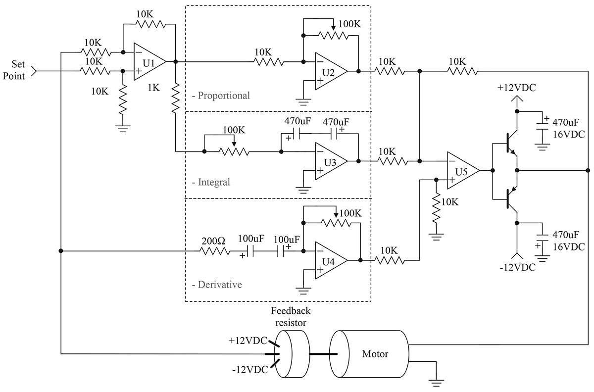

FIGURE 8.

---

This schematic is an adaptation of the PID controller presented by Professor Jacob in his book, Industrial Control Electronics. This type of system has the advantage of easy tuning. This circuit is also simple and easy to construct.
The schematic has the same physical layout as the block diagram. Op-amp U1 is used as the summing junction for the set-point and measured motor position. The individual P, I, and D functions are implemented by U2, U3, and U4, respectively. Finally, op-amp U5 sums the individual PID terms. The P and I terms are inverted, while the D term is not. Darlington transistors have been added to U5 to boost the current to a level sufficient to drive the motor.
The individual P, I, and D components appear just as they were presented earlier in this article. Each of the terms has a variable resistor to adjust its gains. The adjustment (tuning) of this circuit is the topic for the next installment.
Component selection for this circuit is not critical. The variable resistors should be multiturn for ease of adjustment. General-purpose op-amps may be used; however, U3 should be a FET input type. The FET design is better for the integrator, since it will not self-charge the integrator capacitor. I found a quad op-amp — such as the LF347N — to be ideal for this application. Large capacitors are required for the integrator and derivative circuits. The large values necessitate that electrolytic capacitors be used. The electrolytic capacitor may be operated as a non-polarized capacitor by placing two capacitors in series, as shown in the schematic.

Testing

Before we can test the PID circuit, we need to know more about the mechanical system. We need to know how it responds to a command and how the individual P, I, and D terms interact. You will have to be patient and wait for the next installment. In the meantime, go ahead and breadboard the circuit. You can use a function generator to verify the individual stages. See how the individual stages respond to sine, square, and triangle waveforms. Remember to use a low frequency — less than 10 Hz. This frequency is approximately the same as the servo motor system.
Stay tuned; next time, we will learn how to tune the PID controller. We will add additional circuitry to prevent a condition called integral wind-up. Also, keep a lookout for installment three, where we will implement the PID on a ZILOG Encore! microcontroller.


     

                   Analog Electronic PID Controllers  

Although analog electronic process controllers are considered a newer technology than pneumatic process controllers, they are actually “more obsolete” than pneumatic controllers. Panel-mounted (inside a control room environment) analog electronic controllers were a great improvement over panel-mounted pneumatic controllers when they were first introduced to industry, but they were superseded by digital controller technology later on. Field-mounted pneumatic controllers were either replaced by panel-mounted electronic controllers (either analog or digital) or left alone. Applications still exist for field-mounted pneumatic controllers, even now at the beginning of the 21st century, but very few applications exist for analog electronic controllers in any location.  

Analog electronic controllers enjoy only two advantages over digital electronic controllers: greater reliability and faster response. Now that digital industrial electronics has reached a very high level of reliability, the first advantage is academic, leaving only the second advantage for practical consideration. The advantage of faster speed may be fruitful in applications such as motion control, but for most industrial processes even the slowest digital controller is fast enough¹. Furthermore, the numerous advantages offered by digital technology (data recording, networking capability, self-diagnostics,flexible configuration, function blocks for implementing different control strategies) severely weaken the relative importance of reliability and speed.

Most analog electronic PID controllers utilized operational amplifiers in their designs. It is relatively easy to construct circuits performing amplification (gain), integration, differentiation, summation, and other useful control functions with just a few op-amps, resistors, and capacitors.

Circuit design

The following schematic diagram shows a full PID controller implemented using eight operational amplifiers, designed to input and output voltage signals representing PV, SP, and Output:

This controller implements the parallel, or independent PID algorithm, since each tuning adjustment (P, I, and D) act independently of each other:

 

It is possible to construct an analog PID controller with fewer operational amplifiers. An example is shown here:

As you can see, a single operational amplifier does all the work of calculating proportional, integral, and derivative responses. The first three amplifiers do nothing but buffer the input signals and calculate error (PV − SP, or SP − PV, depending on the direction of action).

This controller design happens to implement the series or interacting PID equation. Adjusting either the derivative or integral potentiometers also has an effect on the proportional (gain) value, and adjusting the gain of course has an effect on all terms of the PID equation:

 

It should be apparent to you now why analog controllers tend to implement the series equation instead of the parallel or ideal PID equations: they are simpler and less expensive to build that way.

Single-loop analog controllers

One popular analog electronic controller was the Foxboro model 62H, shown in the following photographs. Like the model 130 pneumatic controller, this electronic controller was designed to fit into a rack next to several other controllers. Tuning parameters were adjustable by moving potentiometer knobs under a side-panel accessible by partially removing the controller from its rack:

 

The Fisher corporation manufactured a series of analog electronic controllers called the AC2, which were similar in construction to the Foxboro model 62H, but very narrow in width so that many could be fit into a compact panel space.

Like the pneumatic panel-mounted controllers preceding, and digital panel-mount controllers to follow, the tuning parameters for a panel-mounted analog electronic controller were typically accessed on the controller’s side. The controller could be slid partially out of the panel to reveal the P, I, and D adjustment knobs (as well as direct/reverse action switches and other configuration controls).

Indicators on the front of an analog electronic controller served to display the process variable (PV), setpoint (SP), and manipulated variable (MV, or output) for operator information. Many analog electronic controllers did not have separate meter indications for PV and SP, but rather used a single meter movement to display the error signal, or difference between PV and SP. On the Foxboro model 62H, a hand-adjustable knob provided both indication and control over SP, while a small edge-reading meter movement displayed the error. A negative meter indication showed that the PV was below setpoint, and a positive meter indication showed that the PV was above setpoint. The Fisher AC2 analog electronic controller used the same basic technique, cleverly applied in such a way that the PV was displayed in real engineering units. The setpoint adjustment was a large wheel, mounted so the edge faced the operator. Along the circumference of this wheel was a scale showing the process variable range, from the LRV at one extreme of the wheel’s travel to the URV at the other extreme of the wheel’s travel. The actual setpoint value was the middle of the wheel from the operator’s view of the wheel edge. A single meter movement needle traced an arc along the circumference of the wheel along this same viewable range. If the error was zero (PV = SP), the needle would be positioned in the middle of this viewing range, pointed at the same value along the scale as the setpoint. If the error was positive, the needle would rise up to point to a larger (higher) value on the scale, and if the error was negative the needle would point to a smaller (lower) value on the scale. For any fixed value of PV, this error needle would therefore move in exact step with the wheel as it was rotated by the operator’s hand. Thus, a single adjustment and a single meter movement displayed both SP and PV in very clear and unambiguous form.

Taylor manufactured a line of analog panel-mounted controllers that worked much the same way, with the SP adjustment being a graduated tape reeled to and fro by the SP adjustment knob. The middle of the viewable section of tape (as seen through a plastic window) was the setpoint value, and a single meter movement needle pointed to the PV value as a function of error. If the error happened to be zero (PV = SP), the needle would point to the middle of this viewable section of tape, which was the SP value.

Another popular panel-mounted analog electronic controller was the Moore Syncro, which featured plug-in modules for implementing different control algorithms (different PID equations, nonlinear signal conditioning, etc.). These plug-in function modules were a hardware precursor to the software “function blocks” appearing in later generations of digital controllers: a simple way of organizing controller functionality so that technicians unfamiliar with computer programming could easily configure a controller to do different types of control functions. Later models of the Syncro featured fluorescent bargraph displays of PV and SP for easy viewing in low-light conditions.

Analog single-loop controllers are largely a thing of the past, with the exception of some low-cost or specialty applications. An example of the former is shown here, a simple analog temperature controller small enough to fit in the palm of my hand:

 

This particular controller happened to be part of a sulfur dioxide analyzer system, controlling the internal temperature of a gas regulator panel to prevent vapors in the sample stream from condensing in low spots of the tubing and regulator system. The accuracy of such a temperature control application was not critical – if temperature was regulated to ±5 degrees Fahrenheit it would be more than adequate. This is an application where an analog controller makes perfect sense: it is very compact, simple, extremely reliable, and inexpensive. None of the features associated with digital PID controllers (programmability, networking, precision) would have any merit in this application.

Multi-loop analog control systems

In contrast to single-loop analog controllers, multi-loop systems control dozens or even hundreds of process loops at a time. Prior to the advent of reliable digital technology, the only electronic process control systems capable of handling the numerous loops within large industrial installations such as power generating plants, oil refineries, and chemical processing facilities were analog systems, and several manufacturers produced multi-loop analog systems just for these large-scale control applications.

One of the most technologically advanced analog electronic products manufactured for industrial control applications was the Foxboro SPEC 200 system². Although the SPEC 200 system used panel-mounted indicators, recorders, and other interface components resembling panel-mounted control systems, the actual control functions were implemented in a separate equipment rack which Foxboro called a nest³. Printed circuit boards plugged into each “nest” provided all the control functions (PID controllers, alarm units, integrators, signal selectors, etc.) necessary, with analog signal wires connecting the various functions together with panel-mounted displays and with field instruments to form a working system.

Analog field instrument signals (4-20 mA, or in some cases 10-50 mA) were all converted to a 0-10 VDC range for signal processing within the SPEC 200 nest. Operational amplifiers (mostly the model LM301) formed the “building blocks” of the control functions, with a +/- 15 VDC power supply providing DC power for everything to operate.

An an example of SPEC 200 technology, the following photographs show a model 2AX+A4 proportional-integral (P+I) controller card, inserted into a metal frame (called a “module” by Foxboro). This module was designed to fit into a slot in a SPEC 200 “nest” where it would reside alongside many other similar cards, each card performing its own control function:

Tuning and alarm adjustments may be seen in the right-hand photograph. This particular controller is set to a proportional band value of approximately 170, and an integral time constant of just over 0.01 minutes per repeat. A two-position rotary switch near the bottom of the card selected either reverse (“Dec”) or direct (“Inc”) control action.

The array of copper pins at the top of the module form the male half of a cable connector, providing connection between the control card and the front-panel instrument accessible to operations personnel. Since the tuning controls appear on the face of this controller card (making it a “card tuned” controller), they were not accessible to operators but rather only to the technical personnel with access to the nest area. Other versions of controller cards (“control station tuned”) had blank places where the P and I potentiometer adjustments appear on this model, with tuning adjustments provided on the panel-mounted instrument displays for easier access to operators.

The set of ten screw terminals at the bottom of the module provided connection points for the input and output voltage signals. The following list gives the general descriptions of each terminal pair, with the descriptions for this particular P + I controller written in italic type:

• Terminals (1+) and (1-): Input signal #1 (Process variable input)

• Terminals (2+) and (2-): Output signal #1 (Manipulated variable output)

• Terminals (3+) and (3-): Input #2, Output #4, or Option #1 (Remote setpoint)

• Terminals (4+) and (4-): Input #3, Output #3, or Option #2 (Optional alarm)

• Terminals (5+) and (5-): Input #4, Output #2, or Option #3 (Optional 24 VAC)

A photograph of the printed circuit board (card) removed from the metal module clearly shows the analog electronic components:

 

Foxboro went to great lengths in their design process to maximize reliability of the SPEC 200 system, already an inherently reliable technology by virtue of its simple, analog nature. As a result, the reliability of SPEC 200 control systems is the stuff of legend⁴.

¹The real problem with digital controller speed is that the time delay between successive “scans” translates into dead time for the control loop. Dead time is the single greatest impediment to feedback control.

²Although the SPEC 200 system – like most analog electronic control systems – is considered obsolete, working installations may still be found at the time of this writing (2008). A report published by the Electric Power Research Institute (see References at the end of this chapter) in 2001 documents a SPEC 200 analog control system installed in a nuclear power plant in the United States as recently as 1992, and another as recently as 2001 in a Korean nuclear power plant.

³Foxboro provided the option of a self-contained, panel-mounted SPEC 200 controller unit with all electronics contained in a single module, but the split architecture of the display/nest areas was preferred for large installations where many dozens of loops (especially cascade, feedforward, ratio, and other multi-component control strategies) would be serviced by the same system.

⁴I once encountered an engineer who joked that the number “200” in “SPEC 200” represented the number of years the system was designed to continuously operate. At another facility, I encountered instrument technicians who were a bit afraid of a SPEC 200 system running a section of their plant: the system had never suffered a failure of any kind since it was installed decades ago, and as a result no one in the shop had any experience troubleshooting it. As it turns out, the entire facility was eventually shut down and sold, with the SPEC 200 nest running faithfully until the day its power was turned off!

          

How PID Controllers Works?  

PID  = proportional + integral and + derivative 

PID Controller is a most common control algorithm used in industrial automation & applications and more than 95% of the industrial controllers are of PID type. PID controllers are used for more precise and accurate control of various parameters.

Most often these are used for the regulation of temperature, pressure, speed, flow and other process variables. Due to robust performance and functional simplicity, these have been accepted by enormous industrial applications where a more precise control is the foremost requirement. Let’s see how the PID controller works.

What is PID Controller?

A combination of proportional, integral and derivative actions is more commonly referred as PID action and hence the name, PID (Proportional-Integral-Derivative)controller. These three basic coefficients are varied in each PID controller for specific application in order to get optimal response.

It gets the input parameter from the sensor which is referred as actual process variable. It also accepts the desired actuator output, which is referred as set variable, and then it calculates and combines the proportional, integral and derivative responses to compute the output for the actuator.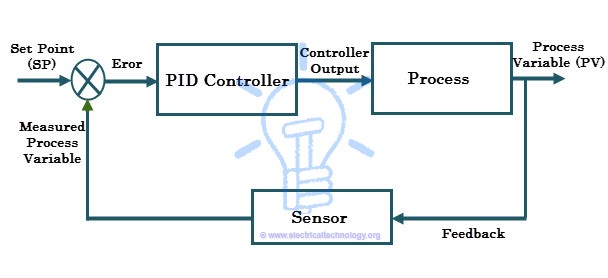Consider the typical control system shown in above figure in which the process variable of a process has to be maintained at a particular level. Assume that the process variable is temperature (in centigrade). In order to measure the process variable (i.e., temperature), a sensor is used (let us say an RTD).

A set point is the desired response of the process. Suppose the process has to be maintained at 80 degree centigrade, and then the set point is 80 degree centigrade. Assume that the measured temperature from the sensor is 50 degree centigrade, (which is nothing but a process variable) but the temperature set point is 80 degree centigrade.

This deviation of actual value from the desired value in the PID control algorithm causes to produce the output to the actuator (here it is a heater) depending on the combination of proportional, integral and derivative responses. So the PID controller continuously varies the output to the actuator till the process variable settle down to the set value. This is also called as closed loop feedback control system.

Working of PID Controller

In manual control, the operator may periodically read the process variable (that has to be controlled such as temperature, flow, speed, etc.) and adjust the control variable (which is to be manipulated in order to bring control variable to prescribed limits such as a heating element, flow valves, motor input, etc.). On the other hand, in automatic control, measurement and adjustment are made automatically on a continuous basis.All modern industrial controllers are of automatic type (or closed loop controllers), which are usually made to produce one or combination of control actions. These control actions include ON-OFF control, proportional control, proportional-integral control, proportional-derivative control and proportional-integral-derivative control.

In case of ON-OFF controller, two states are possible to control the manipulated variable, i.e., either fully ON (when process variable is below the set point) or Fully OFF (when process variable is above the set point). So the output will be of oscillating in nature. In order to achieve the precise control, most industries use the PID controller (or PI or PD depends on the application). Let us look at these control actions.

• Also read: SCADA Systems for Electrical Distribution

P-Control Response

Proportional control or simply P-controller produces the control output proportional to the current error. Here the error is the difference between the set point and process variable (i.e., e = SP – PV). This error value multiplied by the proportional gain (Kc) determines the output response, or in other words proportional gain decides the ratio of proportional output response to error value.

For example, the magnitude of the error is 20 and Kc is 4 then proportional response will be 80. If the error value is zero, controller output or response will be zero. The speed of the response (transient response) is increased by increasing the value of proportional gain Kc. However, if Kc is increased beyond the normal range, process variable starts oscillating at a higher rate and it will cause instability of the system.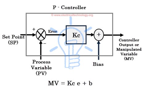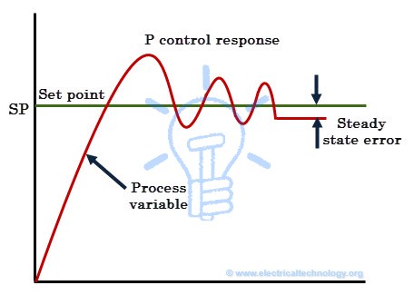Although P-controller provides stability of the process variable with good speed of response, there will always be an error between the set point and actual process variable. Most of the cases, this controller is provided with manual reset or biasing in order to reduce the error when used alone. However, zero error state cannot be achieved by this controller. Hence there will always be a steady state error in the p-controller response as shown in figure.

• Also read: 3 Phase Motor Power & Control Wiring Diagrams

I-Control Response

Integral controller or I-controller is mainly used to reduce the steady state error of the system. The integral component integrates the error term over a period of time until the error becomes zero. This results that even a small error value will cause to produce high integral response. 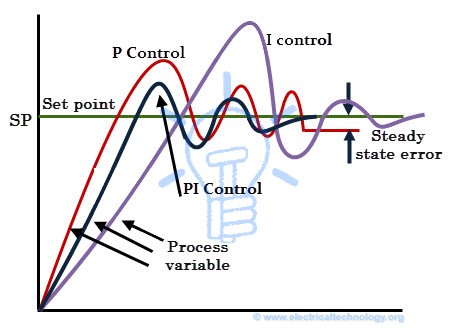At the zero error condition, it holds the output to the final control device at its last value in order to maintain zero steady state error, but in case of P-controller, output is zero when the error is zero.If the error is negative, the integral response or output will be decreased. The speed of response is slow (means respond slowly) when I-controller alone used, but improves the steady state response. By decreasing the integral gain Ki, the speed of the response is increased.For many applications, proportional and integral controls are combined to achieve good speed of response (in case of P controller) and better steady state response (in case of I controller). Most often PI controllers are used in industrial operation in order to improve transient as well as steady state responses. The responses of only I-control, only p-control and PI control are shown in below figure.

D- Controller Response

A derivative controller (or simply D-Controller) sees how fast process variable changes per unit of time and produce the output proportional to the rate of change. The derivative output is equal to the rate of change of error multiplied by a derivative constant. The D-controller is used when the processor variable starts to change at a high rate of speed.

In such case, D-controller moves the final control device (such as control valves or motor) in such direction as to counteract the rapid change of a process variable. It is to be noted that D-controller alone cannot be used for any control applications.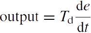

The derivative action increases the speed of the response because it gives a kick start for the output, thus anticipates the future behavior of the error. The more rapidly D-controller responds to the changes in the process variable, if the derivative term is large (which is achieved by increasing the derivative constant or time Td).

In most of the PID controllers, D-control response depends only on process variable, rather than error. This avoids spikes in the output (or sudden increase of output) in case of sudden set point change by the operator. And also most control systems use less derivative time td, as the derivative response is very sensitive to the noise in the process variable which leads to produce extremely high output even for a small amount of noise.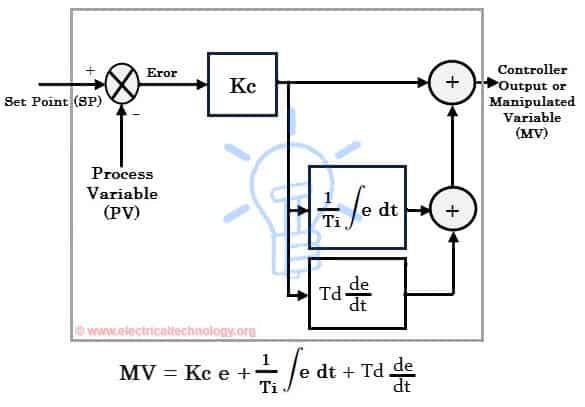

Therefore, by combining proportional, integral, and derivative control responses, a PID controller is formed. A PID controller finds universal application; however, one must know the PID settings and tune it properly to produce the desired output. Tuning means the process of getting an ideal response from the PID controller by setting optimal gains of proportional, integral and derivative parameters.

There are different methods of tuning the PID controller so as to get desired response. Some of these methods include trial and error, process reaction curve technique and Zeigler-Nichols method. Most popularly Zeigler-Nichols and trial and error methods are used.

This is about the PID controller and its working. Due to the simplicity of controller structure, PID controllers are applicable for a variety of processes. And also it can be tuned for any process, even without knowing detailed mathematical model of process. Some of the applications include, PID controller based motor speed control, temperature control, pressure control, flow control, level of the liquid, etc.

• Also read: Arduino Programming: What is Arduino and How to Program it?

Real-time PID Controllers

There are different types PID controllers available in today’s market, which can be used for all industrial control needs such as level, flow, temperature and pressure. When deciding on controlling such parameters for a process using PID, options include use either PLC or standalone PID controller.

Standalone PID controllers are used where one or two loops are needed to be monitored and controlled or in the situations where it difficult to access with larger systems. These dedicated control devices offer a variety of options for single and dual loop control. Standalone PID controllers offer multiple set point configurations and also generates the independent multiple alarms.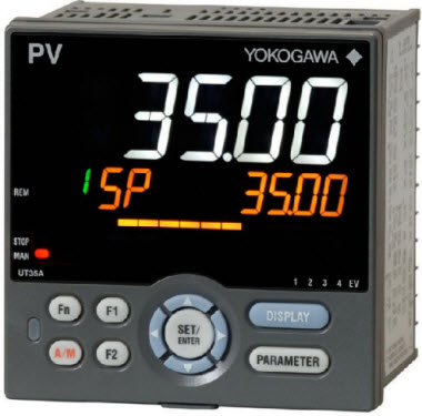

Some of these standalone controllers include Yokogava temperature controllers, Honeywell PID controllers, OMEGA auto tune PID controllers, ABB PID controllers and Siemens PID controllers.

Most of the control applications, PLCs are used as PID controllers. PID blocks are inbuilt in PLCs/PACs and which offers advanced options for a precise control. PLCs are more intelligent and powerful than standalone controllers and make the job easier. Every PLC consist the PID block in their programming software, whether it can Siemens, ABB, AB, Delta, Emersion, or Yokogava PLC.

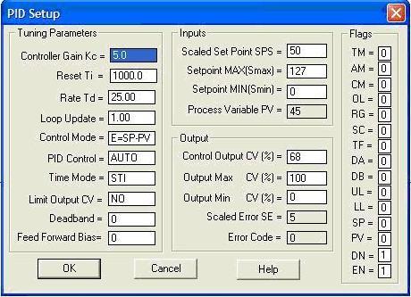
The figure below shows the Allen Bradley (AB) PID block and its setup window.

The figure below shows the Siemens PID block.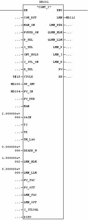

The below figure shows PID controller VIs offered by LabVIEW PID toolset.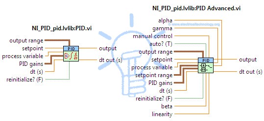

                                    literature study and gauge of appeal 
                     Loving Enter Day on Timing ( LED on T )

Clap Switch Circuit Electronic Project Using 555 Timer & BC-547 Transistors

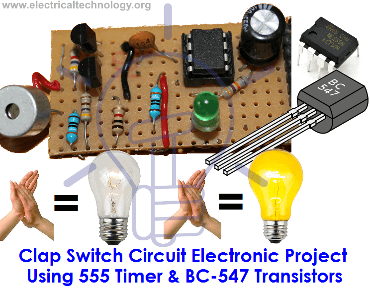
Clap Switch Circuit Electronic Project Using 555 Timer & BC 547 Transistors

Introduction

Clap Switch is a basic Electronics mini-project, made with the help of the basic components. Clap Switch has the ability to turn ON/OFF any electrical component or circuit by the clap sound.

It is known as Clap Switch, because the condenser mic which will be used in this Project will have an ability to take the sound having same pitch as the Clap sound as the input. Although it doesn’t mean that the sound will have to be of Clap sound, it can be any sound having the same high pitch as of Clap. We can also say that it converts the Sound energy into the Electrical Energy, because we are giving an input to the circuit as a sound whereas the Circuit gives us the output as a LED glow (Electrical Energy).

• 
  

Required Components

As already mentioned, this project is basic Electronics mini-project, so this project is made of the basic components. Following is the list of the components required to make the Clap Switch.

1. 1K, 4.7K, 47K, 330 and 470 ohm resistors
2. 10µF and 2 100nF capacitors
3. Electric Condenser mic
4. Two BC547 transistors
5. LED
6. 555 timer
7. 9V Battery

Working Principle of Clap Switch Circuit

This circuit (As shown below) is made with the help of Sound activated sensor, which senses the sound of Clap as input and processes it to the circuit in order to give the Output. When sound is given as the input to the Electric Condenser Mic, it is changed into the Electrical Energy as the LED turns on. LED turns ON, as we give sound input and it turns OFF automatically after few seconds. Turn-On LED timer can be changed by varying the value of 100mF capacitor as it is connected with 555 timer whose main purpose is to generate the pulse.

Although the name of the circuit is the Clap Switch, but you are not restricted to give input as the Clap only. It can be any sound, having same pitch as of Clap so this can also be called as “Sound Operated Switch”. This circuit is mainly based on transistors, because the negative terminal of Mic is directly connected with the transistor. In this circuit, we haven’t used any Electronic Switch to turn on/off the circuit, so when you are connecting the battery with the circuit, it means your circuit is now turned ON and it will take the inputs in the form of Sound Energy. You can modify this circuit by using Relay as Electronic Switch to turn the circuit ON or OFF.

As soon as we give the sound input to the circuit, it amplifies the sound signals and proceeds them to the 555 timers which generates the pulse to the LED, making it turn ON. You are to make sure, that the negative side of the Condenser mic is connected with the amplifier or the circuit will heat-up and may not working with different models of transistors etc. You cannot increase the sensitivity of the Condenser mic for long usage, it has short range by default. It is also applicable for the LAMP, so this circuit has many opportunities for modification.

Clap Switch Circuit Diagram

Advantages & Disadvantages

1. It can used to turn ON and OFF the LED or LAMP simply, by clapping your hands.
2. We can also remove LEDs and place a FAN or any other electric component on the output in order to get desired result.
3. The Condenser Mic used in this circuit has the short range as a default, which cannot be varied.

Applications

Clap Switch is not restricted to turn the LEDs ON and OFF, but it can be used in any electric appliances such as Tube Light, Fan, Radio or any other basic circuit which you want to turn ON by a Sound.

LED String / Strip Circuit Diagram Using PCR-406

It is a very nice and interesting circuit of blinking/Dancing LED String / Strip.
you should try to make one at home because it is very simple and cheep and the basic components of the circuit available everywhere such as an electronics shop. 
This LED Strip/String circuit (Dancing/Blinking LED Circuit) is an interesting circuit where LED bulbs light and glow in different ways like “Dance” and “Blinks” in the following series:

 

• Combination
• In Waves
• Sequential
• Slo-Glo
• Chasing/Flash
• Slow/Fade
• Twinkle/Flash
• Steady On.

so here, we are going step by step to make one of this led blinking and dancing circuit.

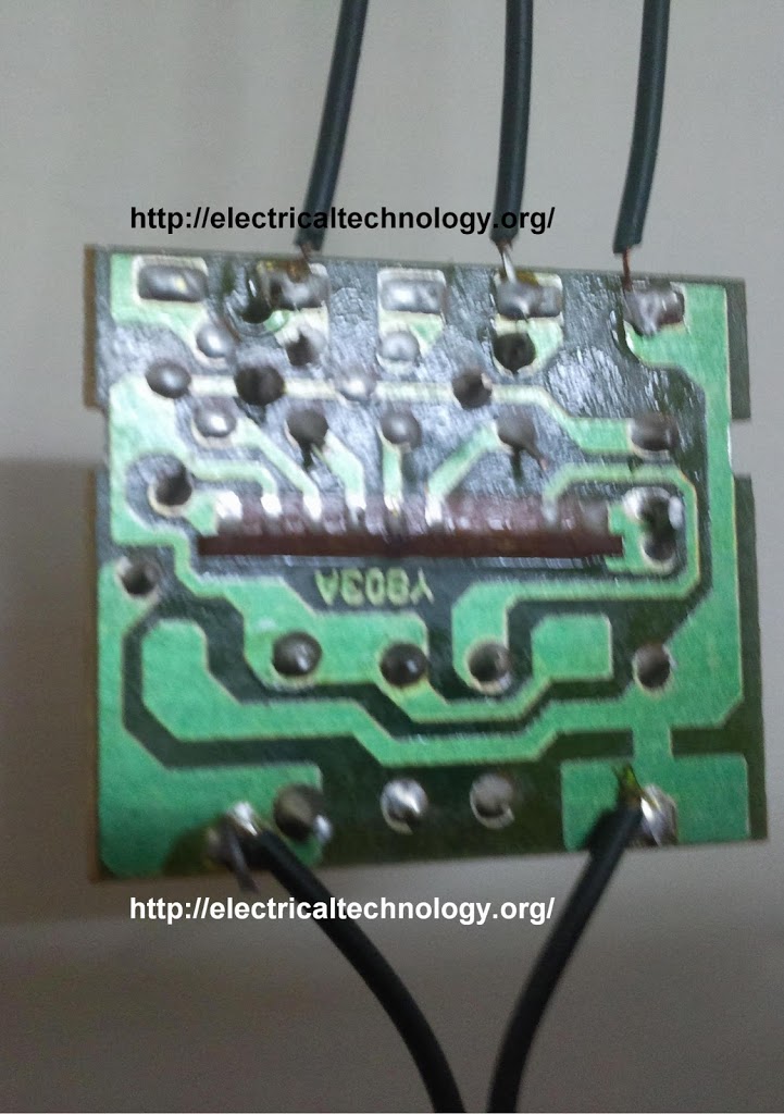
inside the box. this is the basic circuit on general purpose PCB. ( Back Side of the PCB)

Click Image to enlarge

Without Box (different views)

Back view of the Blinking LED Circuit (PCB)

This is the front side of the LED circuit (Front view).

Now turn around the simple  schematic Circuit Diagram of funny LED circuit. it is very simple and easy, DIY (Do it yourself) and homemade. And you must try to make one at home :).

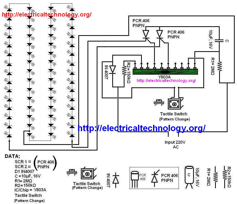
Description of the LED String Circuit.

DATA:
SCR 1 and SCR 2 = PCR 406 PNPN
D1 = IN 4007
C = 10μF, 16 V
R1 = 2MΩ
R2 = 150kΩ
LED = 60 Nos
IC/Chip (Programmable) = Y803A 
Tactile Switch = Pattern Change
Input Voltage
220V, 50-60 Hz

 

when you complete the circuit on general purpose PCB or breadboard, then connect 60 Nos of LED (white or whatever color you want…) … here is the different colors and shapes

We have completed our LED String circuit successfully…

NOW….
Time of  LED STRIP Circuit…One of the most powerful LED Strip/String Circuit Diagram..
you can see some of the following LED Strip images…we will make its Circuit latter after your  review and comments.
Thanks.

Here is some of LED STRIP Images

 

       

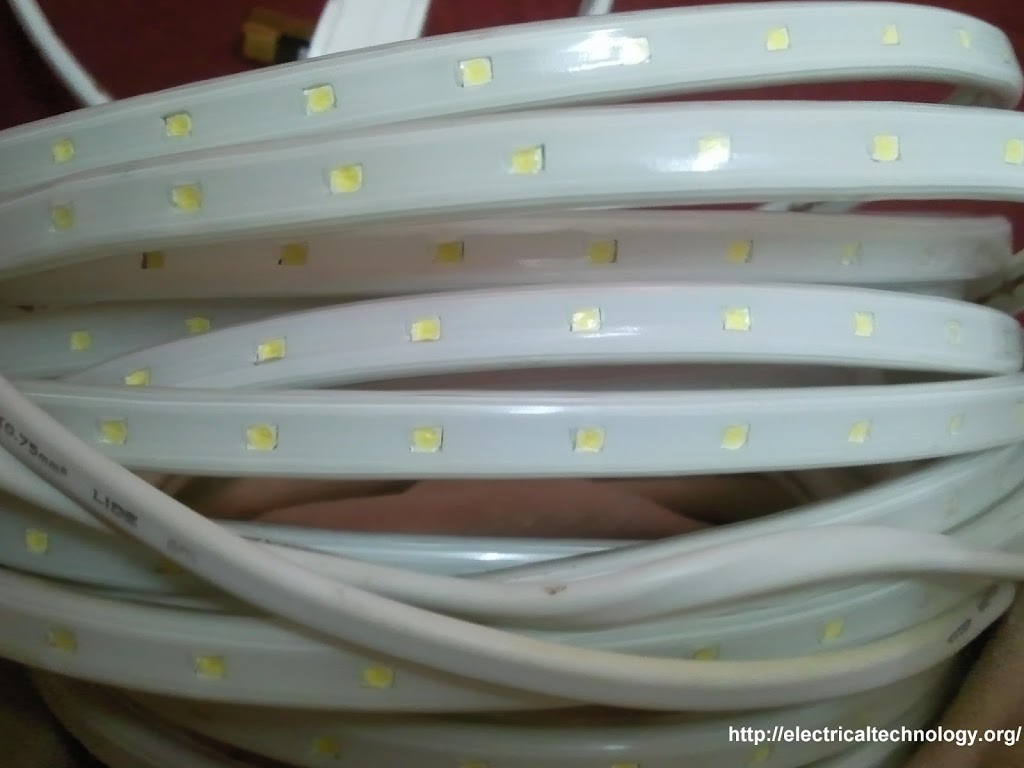
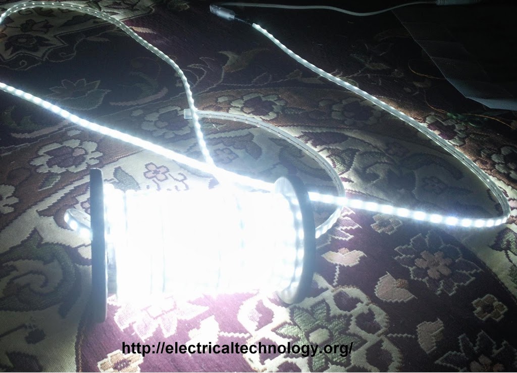
                             XXX  .  XXX 4 zero  Analog and Digital Signals 

Instrumentation is a field of study and work centering on measurement and control of physical processes. These physical processes include pressure, temperature, flow rate, and chemical consistency. An instrument is a device that measures and/or acts to control any kind of physical process. Due to the fact that electrical quantities of voltage and current are easy to measure, manipulate, and transmit over long distances, they are widely used to represent such physical variables and transmit the information to remote locations.

A signal is any kind of physical quantity that conveys information. Audible speech is certainly a kind of signal, as it conveys the thoughts (information) of one person to another through the physical medium of sound. Hand gestures are signals, too, conveying information by means of light. This text is another kind of signal, interpreted by your English-trained mind as information about electric circuits. In this chapter, the word signal will be used primarily in reference to an electrical quantity of voltage or current that is used to represent or signify some other physical quantity.

An analog signal is a kind of signal that is continuously variable, as opposed to having a limited number of steps along its range (called digital). A well-known example of analog vs. digital is that of clocks: analog being the type with pointers that slowly rotate around a circular scale, and digital being the type with decimal number displays or a “second-hand” that jerks rather than smoothly rotates. The analog clock has no physical limit to how finely it can display the time, as its “hands” move in a smooth, pauseless fashion. The digital clock, on the other hand, cannot convey any unit of time smaller than what its display will allow for. The type of clock with a “second-hand” that jerks in 1-second intervals is a digital device with a minimum resolution of one second.

Both analog and digital signals find application in modern electronics, and the distinctions between these two basic forms of information is something to be covered in much greater detail later in this book. For now, I will limit the scope of this discussion to analog signals, since the systems using them tend to be of simpler design.

With many physical quantities, especially electrical, analog variability is easy to come by. If such a physical quantity is used as a signal medium, it will be able to represent variations of information with almost unlimited resolution.

In the early days of industrial instrumentation, compressed air was used as a signaling medium to convey information from measuring instruments to indicating and controlling devices located remotely. The amount of air pressure corresponded to the magnitude of whatever variable was being measured. Clean, dry air at approximately 20 pounds per square inch (PSI) was supplied from an air compressor through tubing to the measuring instrument and was then regulated by that instrument according to the quantity being measured to produce a corresponding output signal. For example, a pneumatic (air signal) level “transmitter” device set up to measure height of water (the “process variable”) in a storage tank would output a low air pressure when the tank was empty, a medium pressure when the tank was partially full, and a high pressure when the tank was completely full.

The “water level indicator” (LI) is nothing more than a pressure gauge measuring the air pressure in the pneumatic signal line. This air pressure, being a signal, is in turn a representation of the water level in the tank. Any variation of level in the tank can be represented by an appropriate variation in the pressure of the pneumatic signal. Aside from certain practical limits imposed by the mechanics of air pressure devices, this pneumatic signal is infinitely variable, able to represent any degree of change in the water’s level, and is therefore analog in the truest sense of the word.

Crude as it may appear, this kind of pneumatic signaling system formed the backbone of many industrial measurement and control systems around the world, and still sees use today due to its simplicity, safety, and reliability. Air pressure signals are easily transmitted through inexpensive tubes, easily measured (with mechanical pressure gauges), and are easily manipulated by mechanical devices using bellows, diaphragms, valves, and other pneumatic devices. Air pressure signals are not only useful for measuring physical processes, but for controlling them as well. With a large enough piston or diaphragm, a small air pressure signal can be used to generate a large mechanical force, which can be used to move a valve or other controlling device. Complete automatic control systems have been made using air pressure as the signal medium. They are simple, reliable, and relatively easy to understand. However, the practical limits for air pressure signal accuracy can be too limiting in some cases, especially when the compressed air is not clean and dry, and when the possibility for tubing leaks exist.

With the advent of solid-state electronic amplifiers and other technological advances, electrical quantities of voltage and current became practical for use as analog instrument signaling media. Instead of using pneumatic pressure signals to relay information about the fullness of a water storage tank, electrical signals could relay that same information over thin wires (instead of tubing) and not require the support of such expensive equipment as air compressors to operate:

Analog electronic signals are still the primary kinds of signals used in the instrumentation world today (January of 2001), but it is giving way to digital modes of communication in many applications (more on that subject later). Despite changes in technology, it is always good to have a thorough understanding of fundamental principles, so the following information will never really become obsolete.

One important concept applied in many analog instrumentation signal systems is that of “live zero,” a standard way of scaling a signal so that an indication of 0 percent can be discriminated from the status of a “dead” system. Take the pneumatic signal system as an example: if the signal pressure range for transmitter and indicator was designed to be 0 to 12 PSI, with 0 PSI representing 0 percent of process measurement and 12 PSI representing 100 percent, a received signal of 0 percent could be a legitimate reading of 0 percent measurement or it could mean that the system was malfunctioning (air compressor stopped, tubing broken, transmitter malfunctioning, etc.). With the 0 percent point represented by 0 PSI, there would be no easy way to distinguish one from the other.

If, however, we were to scale the instruments (transmitter and indicator) to use a scale of 3 to 15 PSI, with 3 PSI representing 0 percent and 15 PSI representing 100 percent, any kind of a malfunction resulting in zero air pressure at the indicator would generate a reading of -25 percent (0 PSI), which is clearly a faulty value. The person looking at the indicator would then be able to immediately tell that something was wrong.

Not all signal standards have been set up with live zero baselines, but the more robust signals standards (3-15 PSI, 4-20 mA) have, and for good reason.

• REVIEW:
• A signal is any kind of detectable quantity used to communicate information.
• An analog signal is a signal that can be continuously, or infinitely, varied to represent any small amount of change.
• Pneumatic, or air pressure, signals used to be used predominately in industrial instrumentation signal systems. This has been largely superseded by analog electrical signals such as voltage and current.
• A live zero refers to an analog signal scale using a non-zero quantity to represent 0 percent of real-world measurement, so that any system malfunction resulting in a natural “rest” state of zero signal pressure, voltage, or current can be immediately recognized. 

    

         Voltage Signal Systems 

the use of variable voltage for instrumentation signals seems a rather obvious option to explore. Let’s see how a voltage signal instrument might be used to measure and relay information about water tank level:

The “transmitter” in this diagram contains its own precision regulated source of voltage, and the potentiometer setting is varied by the motion of a float inside the water tank following the water level. The “indicator” is nothing more than a voltmeter with a scale calibrated to read in some unit height of water (inches, feet, meters) instead of volts.

As the water tank level changes, the float will move. As the float moves, the potentiometer wiper will correspondingly be moved, dividing a different proportion of the battery voltage to go across the two-conductor cable and on to the level indicator. As a result, the voltage received by the indicator will be representative of the level of water in the storage tank.

This elementary transmitter/indicator system is reliable and easy to understand, but it has its limitations. Perhaps greatest is the fact that the system accuracy can be influenced by excessive cable resistance. Remember that real voltmeters draw small amounts of current, even though it is ideal for a voltmeter not to draw any current at all. This being the case, especially for the kind of heavy, rugged analog meter movement likely used for an industrial-quality system, there will be a small amount of current through the 2-conductor cable wires. The cable, having a small amount of resistance along its length, will consequently drop a small amount of voltage, leaving less voltage across the indicator’s leads than what is across the leads of the transmitter. This loss of voltage, however small, constitutes an error in measurement:

Resistor symbols have been added to the wires of the cable to show what is happening in a real system. Bear in mind that these resistances can be minimized with heavy-gauge wire (at additional expense) and/or their effects mitigated through the use of a high-resistance (null-balance?) voltmeter for an indicator (at additional complexity).

Despite this inherent disadvantage, voltage signals are still used in many applications because of their extreme design simplicity. One common signal standard is 0-10 volts, meaning that a signal of 0 volts represents 0 percent of measurement, 10 volts represents 100 percent of measurement, 5 volts represents 50 percent of measurement, and so on. Instruments designed to output and/or accept this standard signal range are available for purchase from major manufacturers. A more common voltage range is 1-5 volts, which makes use of the “live zero” concept for circuit fault indication.

• REVIEW:
• DC voltage can be used as an analog signal to relay information from one location to another.
• A major disadvantage of voltage signaling is the possibility that the voltage at the indicator (voltmeter) will be less than the voltage at the signal source, due to line resistance and indicator current draw. This drop in voltage along the conductor length constitutes a measurement error from transmitter to indicator.

    

        Current Signal Systems 

It is possible through the use of electronic amplifiers to design a circuit outputting a constant amount of current rather than a constant amount of voltage. This collection of components is collectively known as a current source, and its symbol looks like this:

A current source generates as much or as little voltage as needed across its leads to produce a constant amount of current through it. This is just the opposite of a voltage source (an ideal battery), which will output as much or as little current as demanded by the external circuit in maintaining its output voltage constant. Following the “conventional flow” symbology typical of electronic devices, the arrow points against the direction of electron motion. Apologies for this confusing notation: another legacy of Benjamin Franklin’s false assumption of electron flow!

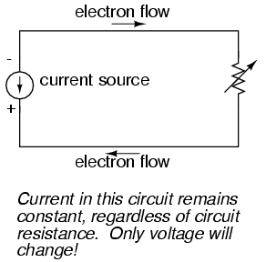
Current sources can be built as variable devices, just like voltage sources, and they can be designed to produce very precise amounts of current. If a transmitter device were to be constructed with a variable current source instead of a variable voltage source, we could design an instrumentation signal system based on current instead of voltage:

The internal workings of the transmitter’s current source need not be a concern at this point, only the fact that its output varies in response to changes in the float position, just like the potentiometer setup in the voltage signal system varied voltage output according to float position.

Notice now how the indicator is an ammeter rather than a voltmeter (the scale calibrated in inches, feet, or meters of water in the tank, as always). Because the circuit is a series configuration (accounting for the cable resistances), current will be precisely equal through all components. With or without cable resistance, the current at the indicator is exactly the same as the current at the transmitter, and therefore there is no error incurred as there might be with a voltage signal system. This assurance of zero signal degradation is a decided advantage of current signal systems over voltage signal systems.

The most common current signal standard in modern use is the 4 to 20 milliamp (4-20 mA) loop, with 4 milliamps representing 0 percent of measurement, 20 milliamps representing 100 percent, 12 milliamps representing 50 percent, and so on. A convenient feature of the 4-20 mA standard is its ease of signal conversion to 1-5 volt indicating instruments. A simple 250 ohm precision resistor connected in series with the circuit will produce 1 volt of drop at 4 milliamps, 5 volts of drop at 20 milliamps, etc:

----------------------------------------
| Percent of  |   4-20 mA  |   1-5 V   |
| measurement |   signal   |   signal  |
----------------------------------------
|      0      |   4.0 mA   |   1.0 V   |
----------------------------------------
|     10      |   5.6 mA   |   1.4 V   |
----------------------------------------
|     20      |   7.2 mA   |   1.8 V   |
----------------------------------------
|     25      |   8.0 mA   |   2.0 V   |
----------------------------------------
|     30      |   8.8 mA   |   2.2 V   |
----------------------------------------
|     40      |  10.4 mA   |   2.6 V   |
----------------------------------------
|     50      |  12.0 mA   |   3.0 V   |
----------------------------------------
|     60      |  13.6 mA   |   3.4 V   |
----------------------------------------
|     70      |  15.2 mA   |   3.8 V   |
----------------------------------------
|     75      |  16.0 mA   |   4.0 V   |
---------------------------------------
|     80      |  16.8 mA   |   4.2 V   |
----------------------------------------
|     90      |  18.4 mA   |   4.6 V   |
----------------------------------------
|    100      |  20.0 mA   |   5.0 V   |
----------------------------------------

The current loop scale of 4-20 milliamps has not always been the standard for current instruments: for a while there was also a 10-50 milliamp standard, but that standard has since been obsoleted. One reason for the eventual supremacy of the 4-20 milliamp loop was safety: with lower circuit voltages and lower current levels than in 10-50 mA system designs, there was less chance for personal shock injury and/or the generation of sparks capable of igniting flammable atmospheres in certain industrial environments.

• REVIEW:
• A current source is a device (usually constructed of several electronic components) that outputs a constant amount of current through a circuit, much like a voltage source (ideal battery) outputting a constant amount of voltage to a circuit.
• A current “loop” instrumentation circuit relies on the series circuit principle of current being equal through all components to insure no signal error due to wiring resistance.
• The most common analog current signal standard in modern use is the “4 to 20 milli amp current loop.”

     

              Tachogenerators 

An electromechanical generator is a device capable of producing electrical power from mechanical energy, usually the turning of a shaft. When not connected to a load resistance, generators will generate voltage roughly proportional to shaft speed. With precise construction and design, generators can be built to produce very precise voltages for certain ranges of shaft speeds, thus making them well-suited as measurement devices for shaft speed in mechanical equipment. A generator specially designed and constructed for this use is called a tachometer or tachogenerator. Often, the word “tach” (pronounced “tack”) is used rather than the whole word.

By measuring the voltage produced by a tachogenerator, you can easily determine the rotational speed of whatever its mechanically attached to. One of the more common voltage signal ranges used with tachogenerators is 0 to 10 volts. Obviously, since a tachogenerator cannot produce voltage when its not turning, the zero cannot be “live” in this signal standard. Tachogenerators can be purchased with different “full-scale” (10 volt) speeds for different applications. Although a voltage divider could theoretically be used with a tachogenerator to extend the measurable speed range in the 0-10 volt scale, it is not advisable to significantly overspeed a precision instrument like this, or its life will be shortened.

Tachogenerators can also indicate the direction of rotation by the polarity of the output voltage. When a permanent-magnet style DC generator’s rotational direction is reversed, the polarity of its output voltage will switch. In measurement and control systems where directional indication is needed, tachogenerators provide an easy way to determine that.

Tachogenerators are frequently used to measure the speeds of electric motors, engines, and the equipment they power: conveyor belts, machine tools, mixers, fans, etc. 

        

              Thermocouples  

An interesting phenomenon applied in the field of instrumentation is the Seebeck effect, which is the production of a small voltage across the length of a wire due to a difference in temperature along that wire. This effect is most easily observed and applied with a junction of two dissimilar metals in contact, each metal producing a different Seebeck voltage along its length, which translates to a voltage between the two (unjoined) wire ends. Most any pair of dissimilar metals will produce a measurable voltage when their junction is heated, some combinations of metals producing more voltage per degree of temperature than others:

The Seebeck effect is fairly linear; that is, the voltage produced by a heated junction of two wires is directly proportional to the temperature. This means that the temperature of the metal wire junction can be determined by measuring the voltage produced. Thus, the Seebeck effect provides for us an electric method of temperature measurement.

When a pair of dissimilar metals are joined together for the purpose of measuring temperature, the device formed is called a thermocouple. Thermocouples made for instrumentation use metals of high purity for an accurate temperature/voltage relationship (as linear and as predictable as possible).

Seebeck voltages are quite small, in the tens of millivolts for most temperature ranges. This makes them somewhat difficult to measure accurately. Also, the fact that any junction between dissimilar metals will produce temperature-dependent voltage creates a problem when we try to connect the thermocouple to a voltmeter, completing a circuit:

The second iron/copper junction formed by the connection between the thermocouple and the meter on the top wire will produce a temperature-dependent voltage opposed in polarity to the voltage produced at the measurement junction. This means that the voltage between the voltmeter’s copper leads will be a function of the difference in temperature between the two junctions, and not the temperature at the measurement junction alone. Even for thermocouple types where copper is not one of the dissimilar metals, the combination of the two metals joining the copper leads of the measuring instrument forms a junction equivalent to the measurement junction:

This second junction is called the reference or cold junction, to distinguish it from the junction at the measuring end, and there is no way to avoid having one in a thermocouple circuit. In some applications, a differential temperature measurement between two points is required, and this inherent property of thermocouples can be exploited to make a very simple measurement system.

However, in most applications the intent is to measure temperature at a single point only, and in these cases the second junction becomes a liability to function.

Compensation for the voltage generated by the reference junction is typically performed by a special circuit designed to measure temperature there and produce a corresponding voltage to counter the reference junction’s effects. At this point you may wonder, “If we have to resort to some other form of temperature measurement just to overcome an idiosyncrasy with thermocouples, then why bother using thermocouples to measure temperature at all? Why not just use this other form of temperature measurement, whatever it may be, to do the job?” The answer is this: because the other forms of temperature measurement used for reference junction compensation are not as robust or versatile as a thermocouple junction, but do the job of measuring room temperature at the reference junction site quite well. For example, the thermocouple measurement junction may be inserted into the 1800 degree (F) flue of a foundry holding furnace, while the reference junction sits a hundred feet away in a metal cabinet at ambient temperature, having its temperature measured by a device that could never survive the heat or corrosive atmosphere of the furnace.

The voltage produced by thermocouple junctions is strictly dependent upon temperature. Any current in a thermocouple circuit is a function of circuit resistance in opposition to this voltage (I=E/R). In other words, the relationship between temperature and Seebeck voltage is fixed, while the relationship between temperature and current is variable, depending on the total resistance of the circuit. With heavy enough thermocouple conductors, currents upwards of hundreds of amps can be generated from a single pair of thermocouple junctions! (I’ve actually seen this in a laboratory experiment, using heavy bars of copper and copper/nickel alloy to form the junctions and the circuit conductors.)

For measurement purposes, the voltmeter used in a thermocouple circuit is designed to have a very high resistance so as to avoid any error-inducing voltage drops along the thermocouple wire. The problem of voltage drop along the conductor length is even more severe here than with the DC voltage signals discussed earlier, because here we only have a few millivolts of voltage produced by the junction. We simply cannot afford to have even a single millivolt of drop along the conductor lengths without incurring serious temperature measurement errors.

Ideally, then, current in a thermocouple circuit is zero. Early thermocouple indicating instruments made use of null-balance potentiometric voltage measurement circuitry to measure the junction voltage. The early Leeds & Northrup “Speedomax” line of temperature indicator/recorders were a good example of this technology. More modern instruments use semiconductor amplifier circuits to allow the thermocouple’s voltage signal to drive an indication device with little or no current drawn in the circuit.

Thermocouples, however, can be built from heavy-gauge wire for low resistance, and connected in such a way so as to generate very high currents for purposes other than temperature measurement. One such purpose is electric power generation. By connecting many thermocouples in series, alternating hot/cold temperatures with each junction, a device called a thermopile can be constructed to produce substantial amounts of voltage and current:

With the left and right sets of junctions at the same temperature, the voltage at each junction will be equal and the opposing polarities would cancel to a final voltage of zero. However, if the left set of junctions were heated and the right set cooled, the voltage at each left junction would be greater than each right junction, resulting in a total output voltage equal to the sum of all junction pair differentials. In a thermopile, this is exactly how things are set up. A source of heat (combustion, strong radioactive substance, solar heat, etc.) is applied to one set of junctions, while the other set is bonded to a heat sink of some sort (air- or water-cooled). Interestingly enough, as electrons flow through an external load circuit connected to the thermopile, heat energy is transferred from the hot junctions to the cold junctions, demonstrating another thermo-electric phenomenon: the so-called Peltier Effect (electric current transferring heat energy).

Another application for thermocouples is in the measurement of average temperature between several locations. The easiest way to do this is to connect several thermocouples in parallel with each other. The millivolt signal produced by each thermocouple will average out at the parallel junction point. The voltage differences between the junctions drop along the resistances of the thermocouple wires:

Unfortunately, though, the accurate averaging of these Seebeck voltage potentials relies on each thermocouple’s wire resistances being equal. If the thermocouples are located at different places and their wires join in parallel at a single location, equal wire length will be unlikely. The thermocouple having the greatest wire length from point of measurement to parallel connection point will tend to have the greatest resistance, and will therefore have the least effect on the average voltage produced.

To help compensate for this, additional resistance can be added to each of the parallel thermocouple circuit branches to make their respective resistances more equal. Without custom-sizing resistors for each branch (to make resistances precisely equal between all the thermocouples), it is acceptable to simply install resistors with equal values, significantly higher than the thermocouple wires’ resistances so that those wire resistances will have a much smaller impact on the total branch resistance. These resistors are called swamping resistors, because their relatively high values overshadow or “swamp” the resistances of the thermocouple wires themselves:

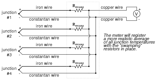
Because thermocouple junctions produce such low voltages, it is imperative that wire connections be very clean and tight for accurate and reliable operation. Also, the location of the reference junction (the place where the dissimilar-metal thermocouple wires join to standard copper) must be kept close to the measuring instrument, to ensure that the instrument can accurately compensate for reference junction temperature. Despite these seemingly restrictive requirements, thermocouples remain one of the most robust and popular methods of industrial temperature measurement in modern use.

• REVIEW:
• The Seebeck Effect is the production of a voltage between two dissimilar, joined metals that is proportional to the temperature of that junction.
• In any thermocouple circuit, there are two equivalent junctions formed between dissimilar metals. The junction placed at the site of intended measurement is called the measurement junction, while the other (single or equivalent) junction is called the reference junction.
• Two thermocouple junctions can be connected in opposition to each other to generate a voltage signal proportional to differential temperature between the two junctions. A collection of junctions so connected for the purpose of generating electricity is called a thermopile.
• When electrons flow through the junctions of a thermopile, heat energy is transferred from one set of junctions to the other. This is known as the Peltier Effect.
• Multiple thermocouple junctions can be connected in parallel with each other to generate a voltage signal representing the average temperature between the junctions. “Swamping” resistors may be connected in series with each thermocouple to help maintain equality between the junctions, so the resultant voltage will be more representative of a true average temperature.
• It is imperative that current in a thermocouple circuit be kept as low as possible for good measurement accuracy. Also, all related wire connections should be clean and tight. Mere millivolts of drop at any place in the circuit will cause substantial measurement errors. 

      

             pH Measurement 

A very important measurement in many liquid chemical processes (industrial, pharmaceutical, manufacturing, food production, etc.) is that of pH: the measurement of hydrogen ion concentration in a liquid solution. A solution with a low pH value is called an “acid,” while one with a high pH is called a “caustic.” The common pH scale extends from 0 (strong acid) to 14 (strong caustic), with 7 in the middle representing pure water (neutral):

pH is defined as follows: the lower-case letter “p” in pH stands for the negative common (base ten) logarithm, while the upper-case letter “H” stands for the element hydrogen. Thus, pH is a logarithmic measurement of the number of moles of hydrogen ions (H+) per liter of solution. Incidentally, the “p” prefix is also used with other types of chemical measurements where a logarithmic scale is desired, pCO2 (Carbon Dioxide) and pO2 (Oxygen) being two such examples.

The logarithmic pH scale works like this: a solution with 10-12 moles of H+ ions per liter has a pH of 12; a solution with 10-3 moles of H+ ions per liter has a pH of 3. While very uncommon, there is such a thing as an acid with a pH measurement below 0 and a caustic with a pH above 14. Such solutions, understandably, are quite concentrated and extremely reactive.

While pH can be measured by color changes in certain chemical powders (the “litmus strip” being a familiar example from high school chemistry classes), continuous process monitoring and control of pH requires a more sophisticated approach. The most common approach is the use of a specially-prepared electrode designed to allow hydrogen ions in the solution to migrate through a selective barrier, producing a measurable potential (voltage) difference proportional to the solution’s pH:

The design and operational theory of pH electrodes is a very complex subject, explored only briefly here. What is important to understand is that these two electrodes generate a voltage directly proportional to the pH of the solution. At a pH of 7 (neutral), the electrodes will produce 0 volts between them. At a low pH (acid) a voltage will be developed of one polarity, and at a high pH (caustic) a voltage will be developed of the opposite polarity.

An unfortunate design constraint of pH electrodes is that one of them (called the measurement electrode) must be constructed of special glass to create the ion-selective barrier needed to screen out hydrogen ions from all the other ions floating around in the solution. This glass is chemically doped with lithium ions, which is what makes it react electrochemically to hydrogen ions. Of course, glass is not exactly what you would call a “conductor;” rather, it is an extremely good insulator. This presents a major problem if our intent is to measure voltage between the two electrodes. The circuit path from one electrode contact, through the glass barrier, through the solution, to the other electrode, and back through the other electrode’s contact, is one of extremely high resistance.

The other electrode (called the reference electrode) is made from a chemical solution of neutral (7) pH buffer solution (usually potassium chloride) allowed to exchange ions with the process solution through a porous separator, forming a relatively low resistance connection to the test liquid. At first, one might be inclined to ask: why not just dip a metal wire into the solution to get an electrical connection to the liquid? The reason this will not work is because metals tend to be highly reactive in ionic solutions and can produce a significant voltage across the interface of metal-to-liquid contact. The use of a wet chemical interface with the measured solution is necessary to avoid creating such a voltage, which of course would be falsely interpreted by any measuring device as being indicative of pH.

Here is an illustration of the measurement electrode’s construction. Note the thin, lithium-doped glass membrane across which the pH voltage is generated:

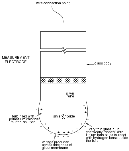
Here is an illustration of the reference electrode’s construction. The porous junction shown at the bottom of the electrode is where the potassium chloride buffer and process liquid interface with each other:

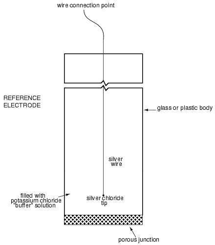
The measurement electrode’s purpose is to generate the voltage used to measure the solution’s pH. This voltage appears across the thickness of the glass, placing the silver wire on one side of the voltage and the liquid solution on the other. The reference electrode’s purpose is to provide the stable, zero-voltage connection to the liquid solution so that a complete circuit can be made to measure the glass electrode’s voltage. While the reference electrode’s connection to the test liquid may only be a few kilo-ohms, the glass electrode’s resistance may range from ten to nine hundred mega-ohms, depending on electrode design! Being that any current in this circuit must travel through both electrodes’ resistances (and the resistance presented by the test liquid itself), these resistances are in series with each other and therefore add to make an even greater total.

An ordinary analog or even digital voltmeter has much too low of an internal resistance to measure voltage in such a high-resistance circuit. The equivalent circuit diagram of a typical pH probe circuit illustrates the problem:

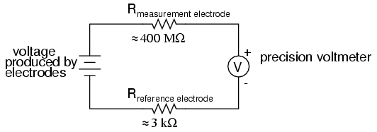
Even a very small circuit current traveling through the high resistances of each component in the circuit (especially the measurement electrode’s glass membrane), will produce relatively substantial voltage drops across those resistances, seriously reducing the voltage seen by the meter. Making matters worse is the fact that the voltage differential generated by the measurement electrode is very small, in the millivolt range (ideally 59.16 millivolts per pH unit at room temperature). The meter used for this task must be very sensitive and have an extremely high input resistance.

The most common solution to this measurement problem is to use an amplified meter with an extremely high internal resistance to measure the electrode voltage, so as to draw as little current through the circuit as possible. With modern semiconductor components, a voltmeter with an input resistance of up to 1017 Ω can be built with little difficulty. Another approach, seldom seen in contemporary use, is to use a potentiometric “null-balance” voltage measurement setup to measure this voltage without drawing any current from the circuit under test. If a technician desired to check the voltage output between a pair of pH electrodes, this would probably be the most practical means of doing so using only standard benchtop metering equipment:

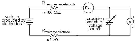
As usual, the precision voltage supply would be adjusted by the technician until the null detector registered zero, then the voltmeter connected in parallel with the supply would be viewed to obtain a voltage reading. With the detector “nulled” (registering exactly zero), there should be zero current in the pH electrode circuit, and therefore no voltage dropped across the resistances of either electrode, giving the real electrode voltage at the voltmeter terminals.

Wiring requirements for pH electrodes tend to be even more severe than thermocouple wiring, demanding very clean connections and short distances of wire (10 yards or less, even with gold-plated contacts and shielded cable) for accurate and reliable measurement. As with thermocouples, however, the disadvantages of electrode pH measurement are offset by the advantages: good accuracy and relative technical simplicity.

Few instrumentation technologies inspire the awe and mystique commanded by pH measurement, because it is so widely misunderstood and difficult to troubleshoot. Without elaborating on the exact chemistry of pH measurement, a few words of wisdom can be given here about pH measurement systems:

• All pH electrodes have a finite life, and that lifespan depends greatly on the type and severity of service. In some applications, a pH electrode life of one month may be considered long, and in other applications the same electrode(s) may be expected to last for over a year.
• Because the glass (measurement) electrode is responsible for generating the pH-proportional voltage, it is the one to be considered suspect if the measurement system fails to generate sufficient voltage change for a given change in pH (approximately 59 millivolts per pH unit), or fails to respond quickly enough to a fast change in test liquid pH.
• If a pH measurement system “drifts,” creating offset errors, the problem likely lies with the reference electrode, which is supposed to provide a zero-voltage connection with the measured solution.
• Because pH measurement is a logarithmic representation of ion concentration, there is an incredible range of process conditions represented in the seemingly simple 0-14 pH scale. Also, due to the nonlinear nature of the logarithmic scale, a change of 1 pH at the top end (say, from 12 to 13 pH) does not represent the same quantity of chemical activity change as a change of 1 pH at the bottom end (say, from 2 to 3 pH). Control system engineers and technicians must be aware of this dynamic if there is to be any hope of controlling process pH at a stable value.
• The following conditions are hazardous to measurement (glass) electrodes: high temperatures, extreme pH levels (either acidic or alkaline), high ionic concentration in the liquid, abrasion, hydrofluoric acid in the liquid (HF acid dissolves glass!), and any kind of material coating on the surface of the glass.
• Temperature changes in the measured liquid affect both the response of the measurement electrode to a given pH level (ideally at 59 mV per pH unit), and the actual pH of the liquid. Temperature measurement devices can be inserted into the liquid, and the signals from those devices used to compensate for the effect of temperature on pH measurement, but this will only compensate for the measurement electrode’s mV/pH response, not the actual pH change of the process liquid!

Advances are still being made in the field of pH measurement, some of which hold great promise for overcoming traditional limitations of pH electrodes. One such technology uses a device called a field-effect transistor to electrostatically measure the voltage produced by an ion-permeable membrane rather than measure the voltage with an actual voltmeter circuit. While this technology harbors limitations of its own, it is at least a pioneering concept, and may prove more practical at a later date.

• REVIEW:
• pH is a representation of hydrogen ion activity in a liquid. It is the negative logarithm of the amount of hydrogen ions (in moles) per liter of liquid. Thus: 10-11 moles of hydrogen ions in 1 liter of liquid = 11 pH. 10-5.3 moles of hydrogen ions in 1 liter of liquid = 5.3 pH.
• The basic pH scale extends from 0 (strong acid) to 7 (neutral, pure water) to 14 (strong caustic). Chemical solutions with pH levels below zero and above 14 are possible, but rare.
• pH can be measured by measuring the voltage produced between two special electrodes immersed in the liquid solution.
• One electrode, made of a special glass, is called the measurement electrode. It’s job it to generate a small voltage proportional to pH (ideally 59.16 mV per pH unit).
• The other electrode (called the reference electrode) uses a porous junction between the measured liquid and a stable, neutral pH buffer solution (usually potassium chloride) to create a zero-voltage electrical connection to the liquid. This provides a point of continuity for a complete circuit so that the voltage produced across the thickness of the glass in the measurement electrode can be measured by an external voltmeter.
• The extremely high resistance of the measurement electrode’s glass membrane mandates the use of a voltmeter with extremely high internal resistance, or a null-balance voltmeter, to measure the voltage. 

     

                Strain Gauges  

If a strip of conductive metal is stretched, it will become skinnier and longer, both changes resulting in an increase of electrical resistance end-to-end. Conversely, if a strip of conductive metal is placed under compressive force (without buckling), it will broaden and shorten. If these stresses are kept within the elastic limit of the metal strip (so that the strip does not permanently deform), the strip can be used as a measuring element for physical force, the amount of applied force inferred from measuring its resistance.

Such a device is called a strain gauge. Strain gauges are frequently used in mechanical engineering research and development to measure the stresses generated by machinery. Aircraft component testing is one area of application, tiny strain-gauge strips glued to structural members, linkages, and any other critical component of an airframe to measure stress. Most strain gauges are smaller than a postage stamp, and they look something like this:

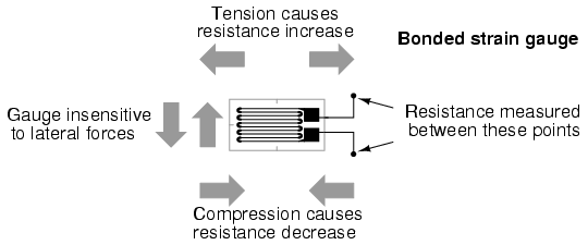
A strain gauge’s conductors are very thin: if made of round wire, about 1/1000 inch in diameter. Alternatively, strain gauge conductors may be thin strips of metallic film deposited on a nonconducting substrate material called the carrier. The latter form of strain gauge is represented in the previous illustration. The name “bonded gauge” is given to strain gauges that are glued to a larger structure under stress (called the test specimen). The task of bonding strain gauges to test specimens may appear to be very simple, but it is not. “Gauging” is a craft in its own right, absolutely essential for obtaining accurate, stable strain measurements. It is also possible to use an unmounted gauge wire stretched between two mechanical points to measure tension, but this technique has its limitations.

Typical strain gauge resistances range from 30 Ω to 3 kΩ (unstressed). This resistance may change only a fraction of a percent for the full force range of the gauge, given the limitations imposed by the elastic limits of the gauge material and of the test specimen. Forces great enough to induce greater resistance changes would permanently deform the test specimen and/or the gauge conductors themselves, thus ruining the gauge as a measurement device. Thus, in order to use the strain gauge as a practical instrument, we must measure extremely small changes in resistance with high accuracy.

Such demanding precision calls for a bridge measurement circuit. Unlike the Wheatstone bridge shown in the last chapter using a null-balance detector and a human operator to maintain a state of balance, a strain gauge bridge circuit indicates measured strain by the degree of imbalance, and uses a precision voltmeter in the center of the bridge to provide an accurate measurement of that imbalance:

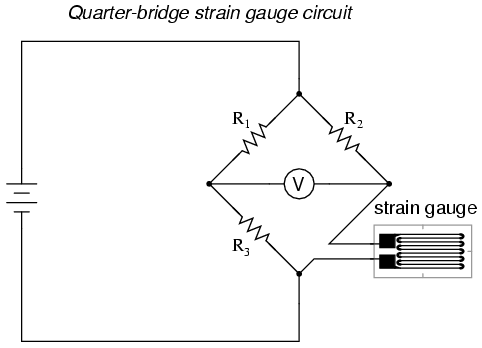
Typically, the rheostat arm of the bridge (R2 in the diagram) is set at a value equal to the strain gauge resistance with no force applied. The two ratio arms of the bridge (R1 and R3) are set equal to each other. Thus, with no force applied to the strain gauge, the bridge will be symmetrically balanced and the voltmeter will indicate zero volts, representing zero force on the strain gauge. As the strain gauge is either compressed or tensed, its resistance will decrease or increase, respectively, thus unbalancing the bridge and producing an indication at the voltmeter. This arrangement, with a single element of the bridge changing resistance in response to the measured variable (mechanical force), is known as a quarter-bridge circuit.

As the distance between the strain gauge and the three other resistances in the bridge circuit may be substantial, wire resistance has a significant impact on the operation of the circuit. To illustrate the effects of wire resistance, I’ll show the same schematic diagram, but add two resistor symbols in series with the strain gauge to represent the wires:

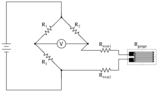
The strain gauge’s resistance (Rgauge) is not the only resistance being measured: the wire resistances Rwire1 and Rwire2, being in series with Rgauge, also contribute to the resistance of the lower half of the rheostat arm of the bridge, and consequently contribute to the voltmeter’s indication. This, of course, will be falsely interpreted by the meter as physical strain on the gauge.

While this effect cannot be completely eliminated in this configuration, it can be minimized with the addition of a third wire, connecting the right side of the voltmeter directly to the upper wire of the strain gauge:

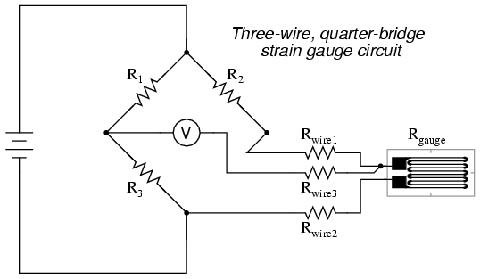
Because the third wire carries practically no current (due to the voltmeter’s extremely high internal resistance), its resistance will not drop any substantial amount of voltage. Notice how the resistance of the top wire (Rwire1) has been “bypassed” now that the voltmeter connects directly to the top terminal of the strain gauge, leaving only the lower wire’s resistance (Rwire2) to contribute any stray resistance in series with the gauge. Not a perfect solution, of course, but twice as good as the last circuit!

There is a way, however, to reduce wire resistance error far beyond the method just described, and also help mitigate another kind of measurement error due to temperature. An unfortunate characteristic of strain gauges is that of resistance change with changes in temperature. This is a property common to all conductors, some more than others. Thus, our quarter-bridge circuit as shown (either with two or with three wires connecting the gauge to the bridge) works as a thermometer just as well as it does a strain indicator. If all we want to do is measure strain, this is not good. We can transcend this problem, however, by using a “dummy” strain gauge in place of R2, so that both elements of the rheostat arm will change resistance in the same proportion when temperature changes, thus canceling the effects of temperature change:

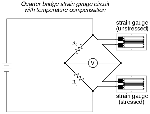
Resistors R1 and R3 are of equal resistance value, and the strain gauges are identical to one another. With no applied force, the bridge should be in a perfectly balanced condition and the voltmeter should register 0 volts. Both gauges are bonded to the same test specimen, but only one is placed in a position and orientation so as to be exposed to physical strain (the active gauge). The other gauge is isolated from all mechanical stress, and acts merely as a temperature compensation device (the “dummy” gauge). If the temperature changes, both gauge resistances will change by the same percentage, and the bridge’s state of balance will remain unaffected. Only a differential resistance (difference of resistance between the two strain gauges) produced by physical force on the test specimen can alter the balance of the bridge.

Wire resistance doesn’t impact the accuracy of the circuit as much as before, because the wires connecting both strain gauges to the bridge are approximately equal length. Therefore, the upper and lower sections of the bridge’s rheostat arm contain approximately the same amount of stray resistance, and their effects tend to cancel:

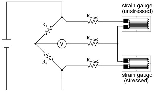
Even though there are now two strain gauges in the bridge circuit, only one is responsive to mechanical strain, and thus we would still refer to this arrangement as a quarter-bridge. However, if we were to take the upper strain gauge and position it so that it is exposed to the opposite force as the lower gauge (i.e. when the upper gauge is compressed, the lower gauge will be stretched, and vice versa), we will have both gauges responding to strain, and the bridge will be more responsive to applied force. This utilization is known as a half-bridge. Since both strain gauges will either increase or decrease resistance by the same proportion in response to changes in temperature, the effects of temperature change remain canceled and the circuit will suffer minimal temperature-induced measurement error:

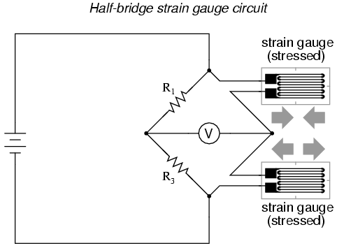
An example of how a pair of strain gauges may be bonded to a test specimen so as to yield this effect is illustrated here:

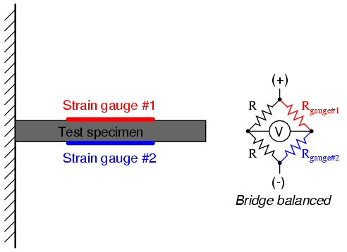
With no force applied to the test specimen, both strain gauges have equal resistance and the bridge circuit is balanced. However, when a downward force is applied to the free end of the specimen, it will bend downward, stretching gauge #1 and compressing gauge #2 at the same time:

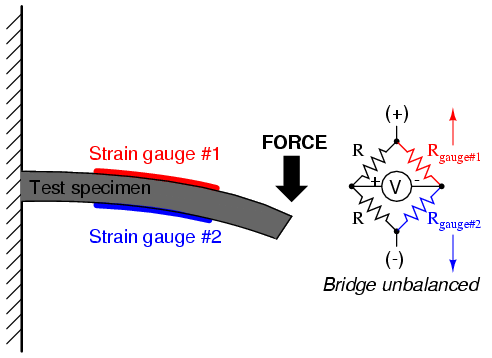
In applications where such complementary pairs of strain gauges can be bonded to the test specimen, it may be advantageous to make all four elements of the bridge “active” for even greater sensitivity. This is called a full-bridge circuit:

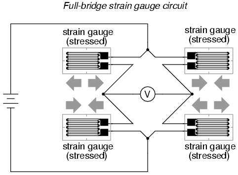
Both half-bridge and full-bridge configurations grant greater sensitivity over the quarter-bridge circuit, but often it is not possible to bond complementary pairs of strain gauges to the test specimen. Thus, the quarter-bridge circuit is frequently used in strain measurement systems.

When possible, the full-bridge configuration is the best to use. This is true not only because it is more sensitive than the others, but because it is linear while the others are not. Quarter-bridge and half-bridge circuits provide an output (imbalance) signal that is only approximately proportional to applied strain gauge force. Linearity, or proportionality, of these bridge circuits is best when the amount of resistance change due to applied force is very small compared to the nominal resistance of the gauge(s). With a full-bridge, however, the output voltage is directly proportional to applied force, with no approximation (provided that the change in resistance caused by the applied force is equal for all four strain gauges!).

Unlike the Wheatstone and Kelvin bridges, which provide measurement at a condition of perfect balance and therefore function irrespective of source voltage, the amount of source (or “excitation”) voltage matters in an unbalanced bridge like this. Therefore, strain gauge bridges are rated in millivolts of imbalance produced per volt of excitation, per unit measure of force. A typical example for a strain gauge of the type used for measuring force in industrial environments is 15 mV/V at 1000 pounds. That is, at exactly 1000 pounds applied force (either compressive or tensile), the bridge will be unbalanced by 15 millivolts for every volt of excitation voltage. Again, such a figure is precise if the bridge circuit is full-active (four active strain gauges, one in each arm of the bridge), but only approximate for half-bridge and quarter-bridge arrangements.

Strain gauges may be purchased as complete units, with both strain gauge elements and bridge resistors in one housing, sealed and encapsulated for protection from the elements, and equipped with mechanical fastening points for attachment to a machine or structure. Such a package is typically called a load cell.

Like many of the other topics addressed in this chapter, strain gauge systems can become quite complex, and a full dissertation on strain gauges would be beyond the scope of this book.

• REVIEW:
• A strain gauge is a thin strip of metal designed to measure mechanical load by changing resistance when stressed (stretched or compressed within its elastic limit).
• Strain gauge resistance changes are typically measured in a bridge circuit, to allow for precise measurement of the small resistance changes, and to provide compensation for resistance variations due to temperature.  

 

Electrical Instrumentation Symbols, Meters and Recorders

The electronic instrumentation are devices for measuring and testing of physical quantities or performance of electrical equipment, circuits or components. They are also used to monitor and control the processes. 

Symbology of Electrical Instrumentation, Meters and Recorders

Symbol	Description		Symbol	Description
	Measuring instrument, meter Generic symbol + info			Measuring instrument, meter + info
	Voltmeter + info			Ammeter + info
	Differential voltmeter			Ammeter with zero center
	Wattmeter + info			Reactive current ammeter
	Wattmeter indicating terminal voltage and current			Ohmmeter + info
	Indicator maximum electricity demand			Frequencymeter + info
	Phase meter / Wavemeter + info			Vu meter + info
	Wavemeter			Thermometer + info
	Phasemeter			Pyrometer + info
	Tachometer + info			Varmeter + info
	Tachometer			Gas meter + info
	Galvanometer + info			Galvanometer
	Oscilloscope / Oscillograph + info			Synchroscope + info
	Oscilloscope / Oscillograph			Salinometer + info
	Oscilloscope with cathode ray tube Shown with electrostatic deflection plates + info			Radiation meter / Geiger counter + info
	Pulse generator + info			Phase comparator
	Waveform generator + info			Probe for measurement and test + info
	Measuring instrument with permanent magnet moving coil			Probe for measurement and test
	Measuring instrument moving coil with rectifier incorporated			Test point + info
	Ionization Chamber + info			Cavity resonator + info
	Thermoluminescent dosimeter + info			Meter quotients
	Scintillation counter + info			Control panel Generic symbol + info
	Telemetry receiver			Telemetry transmitter
	Iron shielding device			Electrodynamic instrument
	Electrodynamic instrument with iron armor			Mobile coil
	Mobile coil with built-in rectifier			Mobile magnet electromagnetic instrument
	Mobile magnet electromagnetic instrument			Mobile iron electromagnetic device
	Electronic device in measuring circuit			Mobile iron electromagnetic device
	Electronic device in auxiliary circuit
Symbols of Counters and Electrical Integrators
	Counter instrument The asterisk is replaced by the letter or symbol for the quantity count + info			Ampere hours meter / Ampere meter + info
	Hourmeter			Watt hour meter / Energy meter + info
	Volt-amperes reactive hours + info			Energy meter with maximum demand indicator
	Energy meter with transmitter			Counter of excess energy
	Energy meter with remote			Energy meter, has the energy flowing toward the bar
	Energy meter with remote and printing			Energy meter, has the energy flowing from the bar
	Energy meter in one direction			Energy meter, has energy in both directions
	Energy meter with dual-rate			Energy meter with recording of maximum demand
	Energy meter with triple rate
Electrical Symbols of Registrars and Recorders
	Recording instrument The asterisk is replaced by the letter or symbol of the magnitude recorded			Ammeter recorder
	Wattmeter recorder			Oscillograph recorder
	Meter and recorder combo counter reactive voltamperes
Symbols Electric Clocks and Timers
	Electric clock Generic symbol + info			Electric clock / Timer + info
	Master clock + info			Time clock + info
	Time Recorder Clock input control			Time clock
	Timer		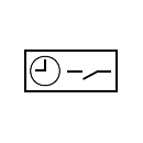	Time switch + info
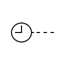	Control timing
Picture gallery of electrical instrumentation, meters and recorders

    

      Good project topics for Electronics and                Instrumentation Engineering

 Engineering Project topics that Electronics & Instrumentation 

1. Animatronics Project
2. Bluetooth Android controlled home appliances using 8051
3. Automatic Street Lighting system using IoT
4. Smart Building Project using PIR
5. Smart Water Monitoring System using IoT
6. Hand Motion Controlled Robotic Arm
7. Embedded System Projects using 8051
8. Weather Monitoring System using IoT
9. Smart Irrigation System using IoT
10. Solar and Smart Energy System
11. IoT using Raspberry Pi for Weather Monitoring
12. Wearable Health Monitoring Glove
13. 3 Phase Induction Motor with Soft Start
14. Smart Energy Meter using GSM
15. Embedded System Projects using 8051
16. Load Control System Using DTMF
17. Automatic Solar Radiation Tracker for Maximum Solar Energy
18. Automatic Room Light Controller using IR Sensors
19. Access control using RFID
20. Biometric Authentication System
21. Speed Controller using Current Sensor for Fans and Coolers
22. Accurate Room Temperature Controller Project
23. Portable Medication Reminder
24. Non-Contact Tachometer using laser
25. Remote Controlled Trolley for Stores Management with Touch Screen
26. Face Recognition System using OpenCV
27. Autonomous Car Parking using GSM
28. Multiplier Accumulator Component VHDL Implementation
29. Controlling Power Grid using PC
30. Wind turbine power generation system - Prototype
31. Scrolling Message Display using Microcontroller
32. Toll Gate System using IOT
33. 3D ultrasonic mouse
34. Data Logger for Solar Panel using Arduino
35. Modelling of the three-phase induction motor using SIMULINK
36. Automatic telephone answering machine
37. Three Phase Rectifier with Power Factor Correction Controller
38. Navigation for Autonomous Wheelchair Robot
39. Biopic Heartbeat Monitor
40. Digital Thermometer Using Temperature Sensor
41. Automatic Toll Tax
42. Auto Answering with Security dialup
43. I2cprotocol Based Real Time Clock Control Application
44. Plotter Robot
45. Function Generator with Frequency Counter
46. Audio DSP: Time and Frequency Varying Gain Compensation for Non-Optimal Listening Levels
47. Programmable Energy Meter for Electrical Load Survey
48. Cable Inspection Robot using Microcontroller and GPS Tracker
49. SCADA control for Remote Industrial Plant
50. Auto Electronics 

                                              XXX  .  XXX 4 zero null 0 1  Clock 

A clock is an instrument to measure, keep, and indicate time. The word clock is derived (via Dutch, Northern French, and Medieval Latin) from the Celtic words clagan and clocca meaning "bell". A silent instrument missing such a striking mechanism has traditionally been known as a timepiece.^[1] In general usage today, a "clock" refers to any device for measuring and displaying the time. Watches and other timepieces that can be carried on one's person are often distinguished from clocks.^[2]

The clock is one of the oldest human inventions, meeting the need to measure intervals of time shorter than the natural units: the day, the lunar month, and the year. Devices operating on several physical processes have been used over the millennia. A sundial shows the time by displaying the position of a shadow on a flat surface. There is a range of duration timers, a well-known example being the hourglass. Water clocks, along with the sundials, are possibly the oldest time-measuring instruments. A major advance occurred with the invention of the verge escapement, which made possible the first mechanical clocks around 1300 in Europe, which kept time with oscillating timekeepers like balance wheels.^[3][4][5][6] Spring-driven clocks appeared during the 15th century. During the 15th and 16th centuries, clockmaking flourished. The next development in accuracy occurred after 1656 with the invention of the pendulum clock. A major stimulus to improving the accuracy and reliability of clocks was the importance of precise time-keeping for navigation. The electric clock was patented in 1840. The development of electronics in the 20th century led to clocks with no clockwork parts at all.

The timekeeping element in every modern clock is a harmonic oscillator, a physical object (resonator) that vibrates or oscillates at a particular frequency.^[4] This object can be a pendulum, a tuning fork, a quartz crystal, or the vibration of electrons in atoms as they emit microwaves. Analog clocks usually indicate time using angles. Digital clocks display a numeric representation of time. Two numeric display formats are commonly used on digital clocks: 24-hour notation and 12-hour notation. Most digital clocks use electronic mechanisms and LCD, LED, or VFD displays. For convenience, distance, telephony or blindness, auditory clocks present the time as sounds. There are also clocks for the blind that have displays that can be read by using the sense of touch. Some of these are similar to normal analog displays, but are constructed so the hands can be felt without damaging them. The evolution of the technology of clocks continues today. The study of timekeeping is known as horology. 

     

Time-measuring devices

Sundials

The apparent position of the Sun in the sky moves over the course of each day, reflecting the rotation of the Earth. Shadows cast by stationary objects move correspondingly, so their positions can be used to indicate the time of day. A sundial shows the time by displaying the position of a shadow on a (usually) flat surface, which has markings that correspond to the hours.^[7] Sundials can be horizontal, vertical, or in other orientations. Sundials were widely used in ancient times.^[8] With the knowledge of latitude, a well-constructed sundial can measure local solar time with reasonable accuracy, within a minute or two. Sundials continued to be used to monitor the performance of clocks until the modern era.^{[citation needed]} However, practical limitations, such as that sundials only work well on relatively clear days, and never during the night, encouraged the development of other techniques for measuring and displaying time. The Jantar Mantar At Delhi and Jaipur are examples of sundials. They were built by Maharaja Jai Singh II.

Devices that measure duration, elapsed time and intervals

The flow of sand in an hourglass can be used to keep track of elapsed time.

Many devices can be used to mark passage of time without respect to reference time (time of day, minutes, etc.) and can be useful for measuring duration or intervals. Examples of such duration timers are candle clocks, incense clocks and the hourglass. Both the candle clock and the incense clock work on the same principle wherein the consumption of resources is more or less constant allowing reasonably precise and repeatable estimates of time passages. In the hourglass, fine sand pouring through a tiny hole at a constant rate indicates an arbitrary, predetermined, passage of time. The resource is not consumed but re-used.

Water

A scale model of Su Song's Astronomical Clock Tower, built in 11th century Kaifeng, China. It was driven by a large waterwheel, chain drive, and escapement mechanism.

Water clocks, also known as clepsydrae (sg: clepsydra), along with the sundials, are possibly the oldest time-measuring instruments, with the only exceptions being the vertical gnomon and the day counting tally stick.^[9] Given their great antiquity, where and when they first existed is not known and perhaps unknowable. The bowl-shaped outflow is the simplest form of a water clock and is known to have existed in Babylon and in Egypt around the 16th century BC. Other regions of the world, including India and China, also have early evidence of water clocks, but the earliest dates are less certain. Some authors, however, write about water clocks appearing as early as 4000 BC in these regions of the world.^[10]

Greek astronomer Andronicus of Cyrrhus supervised the construction of the Tower of the Winds in Athens in the 1st century B.C.^[11] The Greek and Roman civilizations are credited for initially advancing water clock design to include complex gearing, which was connected to fanciful automata and also resulted in improved accuracy. These advances were passed on through Byzantium and Islamic times, eventually making their way back to Europe. Independently, the Chinese developed their own advanced water clocks（水鐘）in 725 A.D., passing their ideas on to Korea and Japan.

Some water clock designs were developed independently and some knowledge was transferred through the spread of trade. Pre-modern societies do not have the same precise timekeeping requirements that exist in modern industrial societies, where every hour of work or rest is monitored, and work may start or finish at any time regardless of external conditions. Instead, water clocks in ancient societies were used mainly for astrological reasons. These early water clocks were calibrated with a sundial. While never reaching the level of accuracy of a modern timepiece, the water clock was the most accurate and commonly used timekeeping device for millennia, until it was replaced by the more accurate pendulum clock in 17th-century Europe.

Islamic civilization is credited with further advancing the accuracy of clocks with elaborate engineering. In 797 (or possibly 801), the Abbasid caliph of Baghdad, Harun al-Rashid, presented Charlemagne with an Asian Elephant named Abul-Abbas together with a "particularly elaborate example" of a water^[12] clock. Pope Sylvester II introduced clocks to northern and western Europe around 1000AD^[13]

An elephant clock in a manuscript by Al-Jazari (1206 AD) from The Book of Knowledge of Ingenious Mechanical Devices.^[14]

In the 13th century, Al-Jazari, an engineer from Mesopotamia (lived 1136–1206) who worked for Artuqid king of Diyar-Bakr, Nasir al-Din, made numerous clocks of all shapes and sizes. A book on his work described 50 mechanical devices in 6 categories, including water clocks. The most reputed clocks included the Elephant, Scribe and Castle clocks, all of which have been successfully reconstructed. As well as telling the time, these grand clocks were symbols of status, grandeur and wealth of the Urtuq State.^{[citation needed]}

Early mechanical

The word horologia (from the Greek ὡρα, hour, and λέγειν, to tell) was used to describe early mechanical clocks,^[15] but the use of this word (still used in several Romance languages) ^[16] for all timekeepers conceals the true nature of the mechanisms. For example, there is a record that in 1176 Sens Cathedral installed a ‘horologe’^[17] but the mechanism used is unknown. According to Jocelin of Brakelond, in 1198 during a fire at the abbey of St Edmundsbury (now Bury St Edmunds), the monks 'ran to the clock' to fetch water, indicating that their water clock had a reservoir large enough to help extinguish the occasional fire.^[18] The word clock (from the Celtic words clocca and clogan, both meaning "bell"), which gradually supersedes "horologe", suggests that it was the sound of bells which also characterized the prototype mechanical clocks that appeared during the 13th century in Europe.

A water-powered cogwheel clock was created in China in AD 725 by Yi Xing and Liang Lingzan. This is not considered an escapement mechanism clock as it was unidirectional, the Song dynasty polymath and genius Su Song (1020–1101) incorporated it into his monumental innovation of the astronomical clock-tower of Kaifeng in 1088.^{[19][page needed]} His astronomical clock and rotating armillary sphere still relied on the use of either flowing water during the spring, summer, autumn seasons and liquid mercury during the freezing temperature of winter (i.e. hydraulics). A mercury clock, described in the Libros del saber, a Spanish work from 1277 consisting of translations and paraphrases of Arabic works, is sometimes quoted as evidence for Muslim knowledge of a mechanical clock. A mercury-powered cogwheel clock was created by Ibn Khalaf al-Muradi^[20][21]

In Europe, between 1280 and 1320, there is an increase in the number of references to clocks and horologes in church records, and this probably indicates that a new type of clock mechanism had been devised. Existing clock mechanisms that used water power were being adapted to take their driving power from falling weights. This power was controlled by some form of oscillating mechanism, probably derived from existing bell-ringing or alarm devices. This controlled release of power—the escapement—marks the beginning of the true mechanical clock, which differed from the previously mentioned cogwheel clocks. Verge escapement mechanism derived in the surge of true mechanical clocks, which didn't need any kind of fluid power, like water or mercury, to work.

These mechanical clocks were intended for two main purposes: for signalling and notification (e.g. the timing of services and public events), and for modeling the solar system. The former purpose is administrative, the latter arises naturally given the scholarly interests in astronomy, science, astrology, and how these subjects integrated with the religious philosophy of the time. The astrolabe was used both by astronomers and astrologers, and it was natural to apply a clockwork drive to the rotating plate to produce a working model of the solar system.

Simple clocks intended mainly for notification were installed in towers, and did not always require faces or hands. They would have announced the canonical hours or intervals between set times of prayer. Canonical hours varied in length as the times of sunrise and sunset shifted. The more sophisticated astronomical clocks would have had moving dials or hands, and would have shown the time in various time systems, including Italian hours, canonical hours, and time as measured by astronomers at the time. Both styles of clock started acquiring extravagant features such as automata.

In 1283, a large clock was installed at Dunstable Priory; its location above the rood screen suggests that it was not a water clock. In 1292, Canterbury Cathedral installed a 'great horloge'. Over the next 30 years there are mentions of clocks at a number of ecclesiastical institutions in England, Italy, and France. In 1322, a new clock was installed in Norwich, an expensive replacement for an earlier clock installed in 1273. This had a large (2 metre) astronomical dial with automata and bells. The costs of the installation included the full-time employment of two clockkeepers for two years.

Astronomical

Richard of Wallingford pointing to a clock, his gift to St Albans Abbey.

16th-century clock machine Convent of Christ, Tomar, Portugal

Besides the Chinese astronomical clock of Su Song in 1088 mentioned above, in Europe there were the clocks constructed by Richard of Wallingford in St Albans by 1336, and by Giovanni de Dondi in Padua from 1348 to 1364. They no longer exist, but detailed descriptions of their design and construction survive,^[22][23] and modern reproductions have been made.^[23] They illustrate how quickly the theory of the mechanical clock had been translated into practical constructions, and also that one of the many impulses to their development had been the desire of astronomers to investigate celestial phenomena.

Wallingford's clock had a large astrolabe-type dial, showing the sun, the moon's age, phase, and node, a star map, and possibly the planets. In addition, it had a wheel of fortune and an indicator of the state of the tide at London Bridge. Bells rang every hour, the number of strokes indicating the time.^[22] Dondi's clock was a seven-sided construction, 1 metre high, with dials showing the time of day, including minutes, the motions of all the known planets, an automatic calendar of fixed and movable feasts, and an eclipse prediction hand rotating once every 18 years.^[23] It is not known how accurate or reliable these clocks would have been. They were probably adjusted manually every day to compensate for errors caused by wear and imprecise manufacture. Water clocks are sometimes still used today, and can be examined in places such as ancient castles and museums. The Salisbury Cathedral clock, built in 1386, is considered to be the world's oldest surviving mechanical clock that strikes the hours.^[24]

Spring-driven

Renaissance Turret Clock, German, circa 1570

Spring driven Matthew Norman carriage clock with winding key

Clockmakers developed their art in various ways. Building smaller clocks was a technical challenge, as was improving accuracy and reliability. Clocks could be impressive showpieces to demonstrate skilled craftsmanship, or less expensive, mass-produced items for domestic use. The escapement in particular was an important factor affecting the clock's accuracy, so many different mechanisms were tried.

Spring-driven clocks appeared during the 15th century,^[25][26][27] although they are often erroneously credited to Nuremberg watchmaker Peter Henlein (or Henle, or Hele) around 1511.^[28][29][30] The earliest existing spring driven clock is the chamber clock given to Phillip the Good, Duke of Burgundy, around 1430, now in the Germanisches Nationalmuseum.^[6] Spring power presented clockmakers with a new problem: how to keep the clock movement running at a constant rate as the spring ran down. This resulted in the invention of the stackfreed and the fusee in the 15th century, and many other innovations, down to the invention of the modern going barrel in 1760.

Early clock dials did not indicate minutes and seconds. A clock with a dial indicating minutes was illustrated in a 1475 manuscript by Paulus Almanus,^[31] and some 15th-century clocks in Germany indicated minutes and seconds.^[32] An early record of a seconds hand on a clock dates back to about 1560 on a clock now in the Fremersdorf collection.^{[33]:417–418[34]}

During the 15th and 16th centuries, clockmaking flourished, particularly in the metalworking towns of Nuremberg and Augsburg, and in Blois, France. Some of the more basic table clocks have only one time-keeping hand, with the dial between the hour markers being divided into four equal parts making the clocks readable to the nearest 15 minutes. Other clocks were exhibitions of craftsmanship and skill, incorporating astronomical indicators and musical movements. The cross-beat escapement was invented in 1584 by Jost Bürgi, who also developed the remontoire. Bürgi's clocks were a great improvement in accuracy as they were correct to within a minute a day.^[35][36] These clocks helped the 16th-century astronomer Tycho Brahe to observe astronomical events with much greater precision than before.

Pendulum

The Dutch polymath and horologist Christiaan Huygens, the inventor of first precision timekeeping devices (pendulum clock and spiral-hairspring watch).^[37]

From its invention in 1656 by Christiaan Huygens until the 1930s, the pendulum clock was the world's most precise timekeeper, accounting for its widespread use.

Pendulum clock Ansonia. C.1904, Ansonia Clock Co., SANTIAGO, hanging oak gingerbread clock, 8-day time and strike.

The next development in accuracy occurred after 1656 with the invention of the pendulum clock. Galileo had the idea to use a swinging bob to regulate the motion of a time-telling device earlier in the 17th century. Christiaan Huygens, however, is usually credited as the inventor. He determined the mathematical formula that related pendulum length to time (about 99.4 cm or 39.1 inches for the one second movement) and had the first pendulum-driven clock made. The first model clock was built in 1657 in the Hague, but it was in England that the idea was taken up.^[38] The longcase clock (also known as the grandfather clock) was created to house the pendulum and works by the English clockmaker William Clement in 1670 or 1671. It was also at this time that clock cases began to be made of wood and clock faces to utilize enamel as well as hand-painted ceramics.

In 1670, William Clement created the anchor escapement,^[39] an improvement over Huygens' crown escapement. Clement also introduced the pendulum suspension spring in 1671. The concentric minute hand was added to the clock by Daniel Quare, a London clockmaker and others, and the second hand was first introduced.

Hairspring

Drawing of one of his first balance springs, attached to a balance wheel, by Christiaan Huygens, published in his letter in the Journal des Sçavants of 25 February 1675. The application of the spiral balance spring (spiral hairspring) for watches ushered in a new era of accuracy for portable timekeepers, similar to that which the pendulum had introduced for clocks.

In 1675, Huygens and Robert Hooke invented the spiral balance, or the hairspring, designed to control the oscillating speed of the balance wheel. This crucial advance finally made accurate pocket watches possible. The great English clockmaker, Thomas Tompion, was one of the first to use this mechanism successfully in his pocket watches, and he adopted the minute hand which, after a variety of designs were trialled, eventually stabilised into the modern-day configuration.^[40] The Rev. Edward Barlow invented the rack and snail striking mechanism for striking clocks, which was a great improvement over the previous mechanism. The repeating clock, that chimes the number of hours (or even minutes) was invented by either Quare or Barlow in 1676. George Graham invented the deadbeat escapement for clocks in 1720.

Marine chronometer

Drawings of Harrison's H4 chronometer of 1761, published in The principles of Mr Harrison's time-keeper, 1767.^[41]

A major stimulus to improving the accuracy and reliability of clocks was the importance of precise time-keeping for navigation. The position of a ship at sea could be determined with reasonable accuracy if a navigator could refer to a clock that lost or gained less than about 10 seconds per day. This clock could not contain a pendulum, which would be virtually useless on a rocking ship. In 1714, the British government offered large financial rewards to the value of 20,000 pounds,^[42] for anyone who could determine longitude accurately. John Harrison, who dedicated his life to improving the accuracy of his clocks, later received considerable sums under the Longitude Act.

In 1735, Harrison built his first chronometer, which he steadily improved on over the next thirty years before submitting it for examination. The clock had many innovations, including the use of bearings to reduce friction, weighted balances to compensate for the ship's pitch and roll in the sea and the use of two different metals to reduce the problem of expansion from heat. The chronometer was tested in 1761 by Harrison's son and by the end of 10 weeks the clock was in error by less than 5 seconds.

Mass production

Eli Terry, the inventor of mass-produced clocks.

The British had predominated in watch manufacture for much of the 17th and 18th centuries, but maintained a system of production that was geared towards high quality products for the elite.^[44] Although there was an attempt to modernise clock manufacture with mass production techniques and the application of duplicating tools and machinery by the British Watch Company in 1843, it was in the United States that this system took off. In 1816, Eli Terry and some other Connecticut clockmakers developed a way of mass-producing clocks by using interchangeable parts.^[45] Aaron Lufkin Dennison started a factory in 1851 in Massachusetts that also used interchangeable parts, and by 1861 was running a successful enterprise incorporated as the Waltham Watch Company.^[46][47]

Early electric

In 1815, Francis Ronalds published the first electric clock powered by dry pile batteries.^[48] Alexander Bain, Scottish clockmaker, patented the electric clock in 1840. The electric clock's mainspring is wound either with an electric motor or with an electromagnet and armature. In 1841, he first patented the electromagnetic pendulum. By the end of the nineteenth century, the advent of the dry cell battery made it feasible to use electric power in clocks. Spring or weight driven clocks that use electricity, either alternating current (AC) or direct current (DC), to rewind the spring or raise the weight of a mechanical clock would be classified as an electromechanical clock. This classification would also apply to clocks that employ an electrical impulse to propel the pendulum. In electromechanical clocks the electricity serves no time keeping function. These types of clocks were made as individual timepieces but more commonly used in synchronized time installations in schools, businesses, factories, railroads and government facilities as a master clock and slave clocks.

Electric clocks that are powered from the AC supply often use synchronous motors. The supply current alternates with a frequency of 50 hertz in many countries, and 60 hertz in others. The rotor of the motor rotates at a speed that is related to the alternation frequency. Appropriate gearing converts this rotation speed to the correct ones for the hands of the analog clock. The development of electronics in the 20th century led to clocks with no clockwork parts at all. Time in these cases is measured in several ways, such as by the alternation of the AC supply, vibration of a tuning fork, the behaviour of quartz crystals, or the quantum vibrations of atoms. Electronic circuits divide these high-frequency oscillations to slower ones that drive the time display. Even mechanical clocks have since come to be largely powered by batteries, removing the need for winding.

Quartz

The piezoelectric properties of crystalline quartz were discovered by Jacques and Pierre Curie in 1880.^[49][50] The first crystal oscillator was invented in 1917 by Alexander M. Nicholson after which, the first quartz crystal oscillator was built by Walter G. Cady in 1921.^[4] In 1927 the first quartz clock was built by Warren Marrison and J. W. Horton at Bell Telephone Laboratories in Canada.^[51][4] The following decades saw the development of quartz clocks as precision time measurement devices in laboratory settings—the bulky and delicate counting electronics, built with vacuum tubes, limited their practical use elsewhere. The National Bureau of Standards (now NIST) based the time standard of the United States on quartz clocks from late 1929 until the 1960s, when it changed to atomic clocks.^[52] In 1969, Seiko produced the world's first quartz wristwatch, the Astron.^[53] Their inherent accuracy and low cost of production resulted in the subsequent proliferation of quartz clocks and watches.^[49]

Atomic

As of the 2010s, atomic clocks are the most accurate clocks in existence. They are considerably more accurate than quartz clocks as they can be accurate to within a few seconds over thousands of years.^[54] Atomic clocks were first theorized by Lord Kelvin in 1879.^[55] In the 1930s the development of Magnetic resonance created practical method for doing this.^[56] A prototype ammonia maser device was built in 1949 at the U.S. National Bureau of Standards (NBS, now NIST). Although it was less accurate than existing quartz clocks, it served to demonstrate the concept.^[57][58][59] The first accurate atomic clock, a caesium standard based on a certain transition of the caesium-133 atom, was built by Louis Essen in 1955 at the National Physical Laboratory in the UK.^[60] Calibration of the caesium standard atomic clock was carried out by the use of the astronomical time scale ephemeris time (ET).^[61] As of 2013, the most stable atomic clocks are ytterbium clocks, which are stable to within less than two parts in 1 quintillion (2×10⁻¹⁸).

Operation

A chiming clock's mechanism.

The invention of the mechanical clock in the 13th century initiated a change in timekeeping methods from continuous processes, such as the motion of the gnomon's shadow on a sundial or the flow of liquid in a water clock, to periodic oscillatory processes, such as the swing of a pendulum or the vibration of a quartz crystal which had the potential for more accuracy. All modern clocks use oscillation.

Although the mechanisms they use vary, all oscillating clocks, mechanical, digital and atomic, work similarly and can be divided into analogous parts. They consist of an object that repeats the same motion over and over again, an oscillator, with a precisely constant time interval between each repetition, or 'beat'. Attached to the oscillator is a controller device, which sustains the oscillator's motion by replacing the energy it loses to friction, and converts its oscillations into a series of pulses. The pulses are then counted by some type of counter, and the number of counts is converted into convenient units, usually seconds, minutes, hours, etc. Finally some kind of indicator displays the result in human readable form.

Power source

Keys of various sizes for winding up mainsprings on clocks.

• In mechanical clocks, the power source is typically either a weight suspended from a cord or chain wrapped around a pulley, sprocket or drum; or a spiral spring called a mainspring. Mechanical clocks must be wound periodically, usually by turning a knob or key or by pulling on the free end of the chain, to store energy in the weight or spring to keep the clock running.
• In electric clocks, the power source is either a battery or the AC power line. In clocks that use AC power, a small backup battery is often included to keep the clock running if it is unplugged temporarily from the wall or during a power outage. Battery powered analog wall clocks are available that operate over 15 years between battery changes.

Oscillator

The timekeeping element in every modern clock is a harmonic oscillator, a physical object (resonator) that vibrates or oscillates repetitively at a precisely constant frequency.^[4]

• In mechanical clocks, this is either a pendulum or a balance wheel.
• In some early electronic clocks and watches such as the Accutron, it is a tuning fork.
• In quartz clocks and watches, it is a quartz crystal.
• In atomic clocks, it is the vibration of electrons in atoms as they emit microwaves.
• In early mechanical clocks before 1657, it was a crude balance wheel or foliot which was not a harmonic oscillator because it lacked a balance spring. As a result, they were very inaccurate, with errors of perhaps an hour a day.

The advantage of a harmonic oscillator over other forms of oscillator is that it employs resonance to vibrate at a precise natural resonant frequency or 'beat' dependent only on its physical characteristics, and resists vibrating at other rates. The possible precision achievable by a harmonic oscillator is measured by a parameter called its Q or quality factor, which increases (other things being equal) with its resonant frequency. This is why there has been a long term trend toward higher frequency oscillators in clocks. Balance wheels and pendulums always include a means of adjusting the rate of the timepiece. Quartz timepieces sometimes include a rate screw that adjusts a capacitor for that purpose. Atomic clocks are primary standards, and their rate cannot be adjusted.

Synchronized or slave clocks

Some clocks rely for their accuracy on an external oscillator; that is, they are automatically synchronized to a more accurate clock:

• Slave clocks, used in large institutions and schools from the 1860s to the 1970s, kept time with a pendulum, but were wired to a master clock in the building, and periodically received a signal to synchronize them with the master, often on the hour.^[71] Later versions without pendulums were triggered by a pulse from the master clock and certain sequences used to force rapid synchronization following a power failure.
• Synchronous electric clocks do not have an internal oscillator, but count cycles of the 50 or 60 Hz oscillation of the AC power line, which is synchronized by the utility to a precision oscillator. The counting may be done electronically, usually in clocks with digital displays, or, in analog clocks, the AC may drive a synchronous motor which rotates an exact fraction of a revolution for every cycle of the line voltage, and drives the gear train. Although changes in the grid line frequency due to load variations may cause the clock to temporarily gain or lose several seconds during the course of a day, the total number of cycles per 24 hours is maintained extremely accurately by the utility company, so that the clock keeps time accurately over long periods.
• Computer real time clocks keep time with a quartz crystal, but can be periodically (usually weekly) synchronized over the Internet to atomic clocks (UTC), using the Network Time Protocol (NTP). Sometimes computers on a local area network (LAN) get their time from a single local server which is maintained accurately.
• Radio clocks keep time with a quartz crystal, but are periodically synchronized to time signals transmitted from dedicated standard time radio stations or satellite navigation signals, which are set by atomic clocks.

Controller

This has the dual function of keeping the oscillator running by giving it 'pushes' to replace the energy lost to friction, and converting its vibrations into a series of pulses that serve to measure the time.

• In mechanical clocks, this is the escapement, which gives precise pushes to the swinging pendulum or balance wheel, and releases one gear tooth of the escape wheel at each swing, allowing all the clock's wheels to move forward a fixed amount with each swing.
• In electronic clocks this is an electronic oscillator circuit that gives the vibrating quartz crystal or tuning fork tiny 'pushes', and generates a series of electrical pulses, one for each vibration of the crystal, which is called the clock signal.
• In atomic clocks the controller is an evacuated microwave cavity attached to a microwave oscillator controlled by a microprocessor. A thin gas of cesium atoms is released into the cavity where they are exposed to microwaves. A laser measures how many atoms have absorbed the microwaves, and an electronic feedback control system called a phase-locked loop tunes the microwave oscillator until it is at the frequency that causes the atoms to vibrate and absorb the microwaves. Then the microwave signal is divided by digital counters to become the clock signal.

In mechanical clocks, the low Q of the balance wheel or pendulum oscillator made them very sensitive to the disturbing effect of the impulses of the escapement, so the escapement had a great effect on the accuracy of the clock, and many escapement designs were tried. The higher Q of resonators in electronic clocks makes them relatively insensitive to the disturbing effects of the drive power, so the driving oscillator circuit is a much less critical component.

Counter chain

This counts the pulses and adds them up to get traditional time units of seconds, minutes, hours, etc. It usually has a provision for setting the clock by manually entering the correct time into the counter.

• In mechanical clocks this is done mechanically by a gear train, known as the wheel train. The gear train also has a second function; to transmit mechanical power from the power source to run the oscillator. There is a friction coupling called the 'cannon pinion' between the gears driving the hands and the rest of the clock, allowing the hands to be turned to set the time.
• In digital clocks a series of integrated circuit counters or dividers add the pulses up digitally, using binary logic. Often pushbuttons on the case allow the hour and minute counters to be incremented and decremented to set the time.

Indicator

A Cuckoo clock with mechanical automaton and sound producer striking on the 8th hour on the analog dial.

This displays the count of seconds, minutes, hours, etc. in a human readable form.

• The earliest mechanical clocks in the 13th century didn't have a visual indicator and signalled the time audibly by striking bells. Many clocks to this day are striking clocks which strike the hour.
• Analog clocks display time with an analog clock face, which consists of a round dial with the numbers 1 through 12, the hours in the day, around the outside. The hours are indicated with an hour hand, which makes two revolutions in a day, while the minutes are indicated by a minute hand, which makes one revolution per hour. In mechanical clocks a gear train drives the hands; in electronic clocks the circuit produces pulses every second which drive a stepper motor and gear train, which move the hands.
• Digital clocks display the time in periodically changing digits on a digital display. A common misconception is that a digital clock is more accurate than an analog wall clock, but the indicator type is separate and apart from the accuracy of the timing source.
• Talking clocks and the speaking clock services provided by telephone companies speak the time audibly, using either recorded or digitally synthesized voices.

Types

Clocks can be classified by the type of time display, as well as by the method of timekeeping.

Time display methods

Analog

A linear clock at London's Piccadilly Circus tube station. The 24 hour band moves across the static map, keeping pace with the apparent movement of the sun above ground, and a pointer fixed on London points to the current time.

A modern quartz clock with a 24-hour face

Analog clocks usually use a clock face which indicates time using rotating pointers called "hands" on a fixed numbered dial or dials. The standard clock face, known universally throughout the world, has a short "hour hand" which indicates the hour on a circular dial of 12 hours, making two revolutions per day, and a longer "minute hand" which indicates the minutes in the current hour on the same dial, which is also divided into 60 minutes. It may also have a "second hand" which indicates the seconds in the current minute. The only other widely used clock face today is the 24 hour analog dial, because of the use of 24 hour time in military organizations and timetables. Before the modern clock face was standardized during the Industrial Revolution, many other face designs were used throughout the years, including dials divided into 6, 8, 10, and 24 hours. During the French Revolution the French government tried to introduce a 10-hour clock, as part of their the decimal-based metric system of measurement, but it didn't catch on. An Italian 6 hour clock was developed in the 18th century, presumably to save power (a clock or watch striking 24 times uses more power).

A simple 24 hour clock showing the approximate position of the sun.

Another type of analog clock is the sundial, which tracks the sun continuously, registering the time by the shadow position of its gnomon. Because the sun does not adjust to daylight savings times, users must add an hour during that time. Corrections must also be made for the equation of time, and for the difference between the longitudes of the sundial and of the central meridian of the time zone that is being used (i.e. 15 degrees east of the prime meridian for each hour that the time zone is ahead of GMT). Sundials use some or part of the 24 hour analog dial. There also exist clocks which use a digital display despite having an analog mechanism—these are commonly referred to as flip clocks. Alternative systems have been proposed. For example, the "Twelv" clock indicates the current hour using one of twelve colors, and indicates the minute by showing a proportion of a circular disk, similar to a moon phase.^[74]

Digital

• Examples of digital clocks
• 

  Digital clock outside Kanazawa Station displaying the time by controlling valves on a fountain
 
• 

  Basic digital clock radio
 
• 

  Mobile phone display with an analog-style clock (albeit generated by a digital computer) in the middle, and a digital-style in the top right corner
 
• 

  Diagram of a mechanical digital display of a flip clock

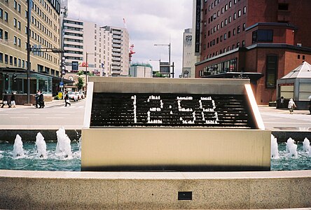
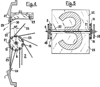
Digital clocks display a numeric representation of time. Two numeric display formats are commonly used on digital clocks:

• the 24-hour notation with hours ranging 00–23;
• the 12-hour notation with AM/PM indicator, with hours indicated as 12AM, followed by 1AM–11AM, followed by 12PM, followed by 1PM–11PM (a notation mostly used in domestic environments).

Most digital clocks use electronic mechanisms and LCD, LED, or VFD displays; many other display technologies are used as well (cathode ray tubes, nixie tubes, etc.). After a reset, battery change or power failure, these clocks without a backup battery or capacitor either start counting from 12:00, or stay at 12:00, often with blinking digits indicating that the time needs to be set. Some newer clocks will reset themselves based on radio or Internet time servers that are tuned to national atomic clocks. Since the advent of digital clocks in the 1960s, the use of analog clocks has declined significantly.

Some clocks, called 'flip clocks', have digital displays that work mechanically. The digits are painted on sheets of material which are mounted like the pages of a book. Once a minute, a page is turned over to reveal the next digit. These displays are usually easier to read in brightly lit conditions than LCDs or LEDs. Also, they do not go back to 12:00 after a power interruption. Flip clocks generally do not have electronic mechanisms. Usually, they are driven by AC-synchronous motors.

Hybrid (analog-digital)

Hybrid real-time animated clock with seconds (12 hours)

Clocks with analog quadrants, with a digital component, usually minutes and hours displayed analogously and seconds displayed in digital mode.

Auditory

For convenience, distance, telephony or blindness, auditory clocks present the time as sounds. The sound is either spoken natural language, (e.g. "The time is twelve thirty-five"), or as auditory codes (e.g. number of sequential bell rings on the hour represents the number of the hour like the bell, Big Ben). Most telecommunication companies also provide a speaking clock service as well.

Word

Software word clock

Word clocks are clocks that display the time visually using sentences. E.g.: "It’s about three o’clock." These clocks can be implemented in hardware or software.

Projection

Some clocks, usually digital ones, include an optical projector that shines a magnified image of the time display onto a screen or onto a surface such as an indoor ceiling or wall. The digits are large enough to be easily read, without using glasses, by persons with moderately imperfect vision, so the clocks are convenient for use in their bedrooms. Usually, the timekeeping circuitry has a battery as a backup source for an uninterrupted power supply to keep the clock on time, while the projection light only works when the unit is connected to an A.C. supply. Completely battery-powered portable versions resembling flashlights are also available.

Tactile

Auditory and projection clocks can be used by people who are blind or have limited vision. There are also clocks for the blind that have displays that can be read by using the sense of touch. Some of these are similar to normal analog displays, but are constructed so the hands can be felt without damaging them. Another type is essentially digital, and uses devices that use a code such as Braille to show the digits so that they can be felt with the fingertips.

Multi-display

Some clocks have several displays driven by a single mechanism, and some others have several completely separate mechanisms in a single case. Clocks in public places often have several faces visible from different directions, so that the clock can be read from anywhere in the vicinity; all the faces show the same time. Other clocks show the current time in several time-zones. Watches that are intended to be carried by travellers often have two displays, one for the local time and the other for the time at home, which is useful for making pre-arranged phone calls. Some equation clocks have two displays, one showing mean time and the other solar time, as would be shown by a sundial. Some clocks have both analog and digital displays. Clocks with Braille displays usually also have conventional digits so they can be read by sighted people.

Purposes

Many cities and towns traditionally have public clocks in a prominent location, such as a town square or city center. This one is on display at the center of the town of Robbins, North Carolina.

Clocks are in homes, offices and many other places; smaller ones (watches) are carried on the wrist or in a pocket; larger ones are in public places, e.g. a railway station or church. A small clock is often shown in a corner of computer displays, mobile phones and many MP3 players.

The primary purpose of a clock is to display the time. Clocks may also have the facility to make a loud alert signal at a specified time, typically to waken a sleeper at a preset time; they are referred to as alarm clocks. The alarm may start at a low volume and become louder, or have the facility to be switched off for a few minutes then resume. Alarm clocks with visible indicators are sometimes used to indicate to children too young to read the time that the time for sleep has finished; they are sometimes called training clocks.

A clock mechanism may be used to control a device according to time, e.g. a central heating system, a VCR, or a time bomb (see: digital counter). Such mechanisms are usually called timers. Clock mechanisms are also used to drive devices such as solar trackers and astronomical telescopes, which have to turn at accurately controlled speeds to counteract the rotation of the Earth.

Most digital computers depend on an internal signal at constant frequency to synchronize processing; this is referred to as a clock signal. (A few research projects are developing CPUs based on asynchronous circuits.) Some equipment, including computers, also maintains time and date for use as required; this is referred to as time-of-day clock, and is distinct from the system clock signal, although possibly based on counting its cycles.

In Chinese culture, giving a clock (送鍾/送钟, sòng zhōng) is often taboo, especially to the elderly as the term for this act is a homophone with the term for the act of attending another's funeral (送終/送终, sòngzhōng).^[75][76][77] A UK government official Susan Kramer gave a watch to Taipei mayor Ko Wen-je unaware of such a taboo which resulted in some professional embarrassment and a pursuant apology.^[78]

It is undesirable to give someone a clock or (depending on the region) other timepiece as a gift. Traditional superstitions regard this as counting the seconds to the recipient's death. Another common interpretation of this is that the phrase "to give a clock" (simplified Chinese: 送钟; traditional Chinese: 送鐘) in Chinese is pronounced "sòng zhōng" in Mandarin, which is a homophone of a phrase for "terminating" or "attending a funeral" (both can be written as 送終 (traditional) or 送终 (simplified)). Cantonese people consider such a gift as a curse.^[79]

This homonymic pair works in both Mandarin and Cantonese, although in most parts of China only clocks and large bells, and not watches, are called "zhong", and watches are commonly given as gifts in China.

However, should such a gift be given, the "unluckiness" of the gift can be countered by exacting a small monetary payment so the recipient is buying the clock and thereby counteracting the '送' ("give") expression of the phrase.

Time standards

For some scientific work timing of the utmost accuracy is essential. It is also necessary to have a standard of the maximum accuracy against which working clocks can be calibrated. An ideal clock would give the time to unlimited accuracy, but this is not realisable. Many physical processes, in particular including some transitions between atomic energy levels, occur at exceedingly stable frequency; counting cycles of such a process can give a very accurate and consistent time—clocks which work this way are usually called atomic clocks. Such clocks are typically large, very expensive, require a controlled environment, and are far more accurate than required for most purposes; they are typically used in a standards laboratory.

Navigation

Until advances in the late twentieth century, navigation depended on the ability to measure latitude and longitude. Latitude can be determined through celestial navigation; the measurement of longitude requires accurate knowledge of time. This need was a major motivation for the development of accurate mechanical clocks. John Harrison created the first highly accurate marine chronometer in the mid-18th century. The Noon gun in Cape Town still fires an accurate signal to allow ships to check their chronometers. Many buildings near major ports used to have (some still do) a large ball mounted on a tower or mast arranged to drop at a pre-determined time, for the same purpose. While satellite navigation systems such as the Global Positioning System (GPS) require unprecedentedly accurate knowledge of time, this is supplied by equipment on the satellites; vehicles no longer need timekeeping equipment.

      What Clock Error Means to Your Measurement System

It's easy to think that clock error only affects your measurement if you're measuring time, but clock error plays a part in many different types of measurements. You may be using a hardware signal to control an analog input scan clock, to time the updates of a waveform generation, or as the counter source clock for a frequency measurement. If your hardware clock signal has clock error, then that error shows up in your measurements.

1. Role of the Clock
2. Components of Clock Error
3. Effects of Clock Error Components
4. Methods of Improvement
5. Improving System Clock Error
6. Conclusion
7. Additional Contributors

1. Role of the Clock

The clock plays a critical role in almost any measurement system. With hardware-timed measurements, the clock controls when the samples or updates occur. You might choose a hardware-timed measurement to achieve a more consistent time interval between samples or updates than you would have if you relied on software to time your measurements. Take, for example, the case of characterizing a digital-to-analog converter (see Figure 1). There are three basic parts to this application -- the digital data stimulus to the digital to analog convertor (DAC), the clock signal, and the digitizer to acquire the analog waveform generated by the DAC. The DAC clocks in a new n-bit word with every rising edge of the clock signal to generate a point in the analog waveform. If the clock signal to the DAC has error, then the analog signal generated by the DAC reflects that error.

Figure 1. DAC Characterization

2. Components of Clock Error

A clock is typically generated by a crystal oscillator, and no oscillator perfectly generates the specified frequency. There are three main components of clock error -- accuracy, stability, and jitter. The clock accuracy describes how well the actual frequency matches the specified frequency. Clock accuracy might be affected by factors such as the quality of the oscillator crystal and how the oscillator was assembled. The clock stability describes how well the oscillator frequency resists fluctuations. The dominant factor that affects stability is a variation in temperature, though aging over time, supply voltage, shock, vibration, and capacitive load that the clock must drive can all affect the clock stability. Jitter refers to small variations in the period of the clock from one edge to the next, and each additional hardware component on the measurement device adds jitter. Figure 2 illustrates the effects of clock accuracy and stability.

Figure 2. Effects of Clock Accuracy and Stability

In each of the diagrams, the dotted line represents the specified, desired frequency, and the solid line represents the actual frequency generated by the oscillator. The upper-left diagram shows an inaccurate and unstable clock; the actual frequency is not centered around the desired frequency, and it changes with respect to time. The upper-right diagram shows an accurate but unstable clock; the actual frequency is centered around the specified frequency but still changes with time. Conversely, the lower-left diagram shows a clock that is inaccurate but stable; the actual frequency is not centered about the desired frequency, but the output frequency from the oscillator does not change over time. A perfect oscillator would generate a frequency like that presented in the lower-right diagram, where the clock is accurate about the desired frequency and does not change with time.

Realistically, if you zoomed in on each diagram, you would see small changes in output frequency from one sample to the next. This apparent noise in the actual frequency generated by the oscillator would represent clock jitter.

3. Effects of Clock Error Components

Assume that the DAC is producing a sine wave of a certain frequency. With a perfect update clock, the frequency domain result would be a single impulse at the fundamental frequency (see Figure 3). If the update clock is inaccurate, then the actual frequency output from the DAC is offset from the desired frequency. If the update clock is accurate but contains jitter, then the output of the DAC contains several frequency components other than the desired fundamental frequency. To illustrate the effects of stability, you would need to examine the frequency domain over time and see how the frequency output of the DAC changes over time.

Figure 3. Effects of Clock Error

4. Methods of Improvement

The clock error is determined by the measurement hardware you choose. To improve your clock error, check the clock error specifications for your device and check the type of oscillator used on your device. Two common types of oscillators are voltage-controlled and oven-controlled oscillators. With a voltage-controlled oscillator (VCXO), the device tunes the output frequency by applying a DC voltage to the oscillator.

With an oven-controlled oscillator (OCXO), an applied voltage controls the output frequency, but an onboard oven maintains a constant internal temperature inside the oscillator. Because the primary contributor to clock instability is temperature variation, controlling the temperature inside the oscillator dramatically increases the clock stability and therefore, greatly improves the overall clock error. By using a device with an OCXO, you can often improve your clock error by a few orders of magnitude.

You can also improve the error from your oscillator by periodically calibrating the timing components of your measurement device. The recommended period between calibration is one year, but you can shorten that period to six months or ninety days depending on the timing precision your application requires. Visit ni.com/calibration for recommended calibration procedures.

5. Improving System Clock Error

You can improve your overall system clock error by sharing a precision clock source among multiple devices in PXI. If you install a PXI device with a low clock error, such as a device with an oven-controlled oscillator, in the PXI star trigger slot (slot 2) and choose devices that implement phase-locked loop (PLL) circuits, then the PXI devices with PLL circuits can take advantage of the high-precision clock of the device in the star trigger slot. A phase-locked loop is a circuit that compares two clocks -- a reference clock and the output of a VCXO.

Figure 4. Phase-Locked Loop

The PLL compares the two clocks and divides the two frequencies to attain a common frequency. For instance, if the PLL is locking a 15 MHz VCXO clock to a 10 MHz reference clock, it may divide the 15 MHz clock by 15 and the 10 MHz clock by 10. Then, it compares the phase and frequency of the two derived 1 MHz clocks and generates a 1 MHz pulse train. The closer matched the two clocks are in frequency and phase, the narrower the pulse widths of the generated 1 MHz pulse train. The pulses are fed to a low pass filter that delivers a DC voltage at its output based on the width of the pulses at its input. This DC voltage is applied to the VCXO to control the output frequency from the VCXO. The PLL works to adjust the DC voltage to minimize the width of the pulses, and to make the frequency and phase of the clock derived from the VCXO match the clock derived from the reference clock. If your measurement devices include phase-locking circuitry, then the device clock inherits the properties of the reference clock in the PLL. If you supply the devices with a high-precision reference clock, then your other phase-locking devices can take advantage of that high-precision clock throughout your PXI measurement system.

p

6. Conclusion

Understanding the components of clock error allows you to better understand your measurements. No measurement system is free of clock error, but there are some steps you can take to minimize the clock error per measurement device or throughout your measurement system. You can choose measurement devices with high-precision oscillators like an OCXO, and choose measurement systems like phase-locking devices in PXI that can share the clock from that high-precision oscillator. Periodic timing calibration of your measurement devices also minimizes the clock error from their oscillators. By understanding the implications of clock error and implementing some of these methods, you can achieve the timing precision required in your measurement application.

7. Additional Contributors

June Zhe received her Bachelor of Science for Electrical Engineering from Rensselaer Polytechnic Institute. Currently, she is a Product Support Engineer in the Digital and Timing group at National Instruments. Her areas of expertise include customer support and usability of digital and counter/timer products.

Cory Wile received his Bachelor of Science for Electrical Engineering from the University of Texas at Austin. Currently, he is a Hardware Design Engineer in the Digital and Timing group at National Instruments. His areas of expertise include counter/timer products, microprocessors, VHDL design, and device production tests. 

ATOMIC TIME?

Variations and vagaries in the Earth's rotation eventually made astronomical measurements of time inadequate for scientific and military needs that required highly accurate timekeeping. Today's standard of time is based on atomic clocks that operate on the frequency of internal vibrations of atoms within molecules. These frequencies are independent of the Earth's rotation, and are consistent from day to day within one part in 1,000 billion. 

                                                   

Synchronization with a Sample Clock

The master device can control operation of the measurement system by exporting both trigger signals and a sample clock to the slave devices. For example, a system comprised of multiple digitizers and signal generators has a common sample clock from an appointed master device. As illustrated in Figure 3, the master sample clock directly controls ADC and DAC timing on all devices. For example, National Instruments dynamic signal analyzers such as the NI 4472 and NI 4461 (24-bit 104 kS/s and 208 kS/s respectively) are synchronized using this technique for applications in sound and vibration measurements.

This scheme is the purest form of phase-coherent sampling; multiple devices are fed the same sample clock. Thus the same accuracy, drift, and jitter of the sample clock are seen by every device. The disadvantage of this scheme is that it does not address all possible phase-coherent heterogeneous clocking needs.

Figure 3. Synchronization with a Sample Clock

Synchronization Scheme 2 – Synchronization with a Reference Clock

Synchronization can be implemented by sharing triggers and reference clocks between multiple measurement devices. In this scheme, the reference clock can be supplied by the master device if it has an onboard reference clock, or the reference clock can be supplied by a dedicated high-precision clock source.

This advantage of this scheme is that with it you can derive heterogeneous sample clocks from a single reference clock to which all the sample clocks phase locked. The trade-off is that the phase-coherent sampling on each device is not as pure as the direct sample clock approach, because each device clock enters the picture, so device clock jitter must be considered.

The method usually employed with this scheme to synchronize and generate sampling clocks is a PLL.

Figure 4. Synchronization with a Reference Clock

Figure 5. High-speed sample clocks are synchronized using a PLL.

Distributing clocks and triggers to achieve high-speed synchronized devices is beset by nontrivial issues. Latencies and timing uncertainties involved in orchestrating multiple-measurement devices are significant challenges in synchronization, especially for high-speed measurement systems. These issues, often overlooked during the initial system design, limit the speed and accuracy of synchronized systems. Two main issues that arise in the distribution of clocks and triggers are skew and jitter.4. Issues with Synchronization

Sample Clock Synchronization

Mixed-signal test by its nature requires different sampling rates on each instrument, because analog waveform I/O and digital waveform I/O necessitate different sampling rates. But they need to be synchronized, and more importantly data needs to be sampled on the correct sample clock edge on each instrument.

When sample clocks on disparate instruments are integer multiples of the 10 MHz reference clock, all instruments will have sample clocks that are synchronous to each other – the rising edge of all sample clocks will be coincident with the 10 MHz clock edge. When sample clocks are not integer multiples, such as 25 MHz, there is no guarantee that the sample clocks are in phase, despite being phase-locked to the 10 MHz reference clock, as shown in Figure 6. Standard techniques are used to solve this problem by resetting all of the PLLs at the same time, leading to sample clocks of the same frequency being in phase, as shown in Figure 7. Even though all sample clocks are in phase at this point, the solution is still not complete. Perfect synchronization implies the data clocked from device to device corresponding to within a sample clock cycle. The key to perfect synchronization is triggering, which will be discussed later.

Figure 6. 25 MHz Sample Clocks Not Aligned

Figure 7. PLL Synchronization with Reset

Clock Skew and Jitter

The distribution of the sample clock or the reference clock requires careful planning. For example, a synchronized measurement system calls for simultaneous sampling of 20 channels at 200 MS/s. This requirement implies distributing a clock to 10 two-channel digitizers. For a sample clock skew of 1%, the skew must be under 25 ps. Such a system certainly looks very challenging. Fortunately, skew limitations can be dealt with by calibrating the skew to each measurement device; you can compensate for the skew in the sampled data. The real issue is the clock frequency . Distributing either a 200 MHz direct sample clock or a 10 MHz reference clock introduces jitter into the system. The physical properties of the distribution system play a significant role in the accuracy of the distributed clocks; if the clock paths are susceptible to high-frequency electrical noise then clock jitter becomes a significant problem. Producing a platform for distribution of high-frequency sample clocks becomes expensive in terms of the manufacture, test, and calibration. Thus synchronization through the use of lower frequency reference clocks is the preferred method in many high-frequency systems. Figure 8 is a typical VCXO PLL implemented on National Instruments SMC-based modular instruments. The loop bandwidth is kept at a minimum to reject the jitter coming from the reference clock, while the VCXO on the device has jitter less then 1 psrms. Such a system effectively realizes a low-jitter synchronized system.

A very useful property of the National Instruments PLL design is the use of a phase DAC. Using a phase DAC, you can phase-align the output of the VCXO with respect to the incoming reference clock. Nominally the VCXO output is in phase with the reference clock; however, you may need to skew the VCXO output slightly to place the output out of phase by a small margin. This feature is important for aligning sample clocks on multiple devices when the reference clock fed to each device has a small skew due to propagation delays. For example, in the NI PXI-1042 PXI chassis, the distribution of 10 MHz reference clock has slot-to-slot skew of 250 ps maximum with a maximum of 1 psrms jitter. Slot-to-slot skew of 250 ps, while satisfactory for most applications, may not be adequate for very high-speed applications where phase accuracy is important. To overcome this skew, the phase DAC outputs can be adjusted to calibrate for the skew. On the NI PXI-5422, 200 MS/s arbitrary waveform generator and NI PXI-5124 200 MS/s digitizer the sample clock phase/delay adjustment is 5 ps, thus giving the user significant flexibility in synchronizing multiple devices.

Figure 8. PLL with Phase Adjustment DAC for Flexibility in Sample Clock Delay with Respect to the Reference Clock

Trigger Skew and Distribution

With sample clock synchronization addressed, the other main issue is the distribution of the trigger to initiate simultaneous operation. The trigger can come from a digital event or from an analog signal that meets trigger conditions. Typically in multichannel systems, one of the devices is made the master and the rest are designated as slaves. In this scenario, the master is programmed to distribute the trigger signal to all slaves in the system including itself. Two issues that arise here are trigger delay and skew. A trigger delay from the master to all the slaves and skew between each slave device is inevitable, but this delay and skew can be measured and calibrated.

The challenge in measuring the delay and skew, however, is a two-part process:

1. Automate the measurement of the trigger delay between master and each slave and compensate for it.
2. Ensure that the skew between slaves is small enough to ensure that the trigger is seen on the same clock edge on all devices.

The distribution of the trigger signal across multiple devices requires passing a trigger signal into the clock domain of the sample clock such that the trigger is seen at the right instance in time on each device.

With sample clock rates less than or equal to 100 MS/s, skew becomes a major obstacle to accurate trigger distribution. A system consisting of ten 200 MS/s devices, for example, requires a trigger being received at each device within a 5 ns window. This places a significant burden on the platform for delivering T&S beyond 100 MHz. The trigger signals must be sent in a slower clock domain than that of sample clock, or you must create a nonbused means of sending the trigger signal (such as a point-to-point connection). The costs of such a platform become prohibitive for mainstream use. Another distribution channel is needed; the trigger signal needs to be distributed reliably using a slow clock domain and transferred to the high-speed sample clock domain. A logical choice is to synchronize the trigger signal distribution with the 10 MHz reference clock. However, this cannot ensure that two boards will see the trigger assertion in the same sample clock cycle when the sample clocks are not integer multiples of the 10 MHz reference clock. To illustrate this point, assume two devices have the simple circuit [4] shown in Figure 9 for trigger transfer from the 10 MHz reference clock domain to the sample clock domain.

Figure 9. 10 MHz Reference Clock Domain to Sample Clock Domain Trigger Transfer

Even if the sample clocks of the devices are aligned, the following timing diagram shows why the trigger may not be seen in the same sample clock cycle on both devices.

Figure 10. Effect of Metastability on Triggers

The output of the first flip-flop (cTrig) may occur too close to the rising edge of the sample clock, causing mTrig to be metastable. When the metastability finally settles, it may do so differently on different devices, causing them to see the same trigger signal at two different instants in time.

In 2003, National Instruments introduced the first series of PXI digitizers, arbitrary waveform generators, and digital pattern generators/analyzers based on the Synchronization and Memory Core (SMC) foundation [5]. One of the key technologies implemented on the SMC was NI-TClk (pronounced T-Clock) technology for T&S applications.5. SMC Modular Instrumentation and NI-TClk

NI-TClk

National Instruments has developed a patent-pending method for synchronization whereby another signal-clock domain is employed to enable alignment of sample clocks and the distribution and reception of triggers. The objectives of NI-TClk technology are twofold:

• NI-TClk aligns the sample clocks that may not be necessarily aligned initially despite being phase locked to the 10 MHz reference clock.
• NI-TClk enables accurate triggering of synchronized devices.

NI-TClk synchronization is flexible and wide ranging; it can address the following use cases:

• Extension of synchronization from a single PXI chassis to several PXI chassis to address large channel systems using the NI PXI-6653 Slot 2 system timing and control module.
• Homogeneous and heterogeneous synchronization – devices running at the same or different sample rates, using internal or external sample clocks.
• NI-TClk synchronization can be used with both Schemes 1 and 2, as described previously.

Figure 11. Illustration of multichassis synchronization that uses the NI PXI-6653 system timing and control module whereby the 10 MHz reference clock and triggers are distributed from a master chassis to all slave chassis, with NI MXI-4 controlling all slave chassis.

The purpose of NI-TClk synchronization is to have devices respond to triggers at the same time. The "same time" means on the same sample period and having very tight alignment of the sample clocks. NI-TClk synchronization is accomplished by having each device generate a trigger clock (TClk) that is derived from the sample clock. Triggers are synchronized to a TClk pulse. A device that receives a trigger from an external source or generates it internally will send the signal to all devices, including itself, on a falling edge of TClk. All devices react to the trigger on the following rising edge of TClk. The TClk frequency is much lower then the sample clock and the PXI 10 MHz reference clock to accommodate the NI PXI-1045 18-slot chassis, where the propagation delay from Slot 1 to Slot 18 may extend to several nanoseconds. If the application calls for multiple chassis where the propagation delay can be higher then normal interchassis delay, you can set the TClk frequency.

The issue of "instantaneous" data acquisition comes up; if a trigger condition is met and 10 digitizers are required to be triggered, the issue of latency arises due to the synchronization of the trigger to TClk. This issue is addressed with pretrigger and posttrigger samples on the device sample memory buffer. All NI-TClk supported devices are programmed to accommodate the overhead time that arises from synchronization of the trigger to the TClk. For example, 10 digitizers are programmed to acquire 10,000 samples simultaneously. The sample rate is 200 MS/s (sample period of 5 ns) from which the derived TClk frequency is programmed to be 5 MHz (sample period of 200 ns). This implies that the delay in acquisition resulting from TClk synchronization of the trigger could be as high as 40 samples. NI-TClk supported devices are programmed to automatically pad the memory buffer for the lag between the trigger event and the start of acquisition, and the NI-TClk driver software automatically adjusts the timestamps on all digitizers to reflect the start of acquisition with respect to the trigger event.

Overview of NI-TClk Operation with an Internal (PXI) Reference Clock or User-Supplied Reference Clock

The devices are synchronized in the following manner. Refer to Figure 12 for the timing diagram that illustrates sample clock alignment and Figure 13 for trigger distribution and reception.

1. Each device is programmed with a sample clock rate, and set to receive the TClk trigger.
2. NI-TClk software automatically calculates the TClk frequency based on the sample clocks and number of devices involved, and TClks are generated on each device, derived from the sample clocks of the devices.
3. The PXI 10 MHz reference clock (in PCI the onboard reference clock of one of the devices is used) is distributed to all devices to phase-lock the sample clocks on all devices.
4. Each device sample clock is phase-locked to the 10 MHz reference clock but is not necessarily in phase with each other at this stage.
5. A common clock signal called the Sync Pulse Clock is distributed through the PXI trigger bus (over the RTSI bus for PCI boards) to all devices whose frequency is similar to the reference clock frequency. Here the 10 MHz reference clock plays the role of the Sync Pulse Clock in addition to being the reference clock.
6. A Sync Pulse is generated from one of the devices when the Sync Pulse Clock (10 MHz reference clock) is logically high through the PXI trigger bus (over the RTSI bus for PCI boards).
7. Each device is initiated to look for the first rising edge of the Sync Pulse Clock upon receiving the Sync Pulse.
8. When the first rising edge of the Sync Pulse Clock is detected, each device is programmed to measure the time between this edge and the first rising edge of the device TClk. The time between these two edges is measured on all devices.
9. TClk measurements of all devices are compared to one reference TClk measurement (the NI-TClk driver software automatically selects one of the devices), and all device sample clocks and TClks are aligned automatically by adjusting the phase DAC outputs on all devices.
10. With the sample clocks on all devices aligned, the trigger signal is distributed from the appointed master to all other devices through the TClk. The trigger signal is emitted with the falling edge of the master device TClk, and all devices are programmed to initiate generation or acquisition with the next rising edge of TClk. This signal is also distributed through the PXI trigger bus (over the RTSI bus for PCI boards). See Figure 13.

Two Properties of NI-TClk Synchronization are critical to the success of the method:

• The distribution of the Sync Pulse is critical to NI-TClk synchronization. The Sync Pulse must arrive at each device such that each device looks for the same rising edge of the Sync Clock Pulse in making the TClk measurement. The skew cannot exceed the period of the Sync Pulse Clock. This issue is easily resolved with the Sync Pulse Clock period being 100 ns. NI-TClk synchronization can easily extend from synchronization within one chassis to several dozen, as the standard delay per foot of 50 Ω cable is of the order of 2 ns.
• The accuracy of the sample clock alignment is as good as the skew of the Sync Pulse Clock (reference clock). In looking at Figure 12, you can see that the reference clock received on both devices is skewed. The TClk measurements on both devices assume that the Sync Pulse Clock is aligned on both devices; the difference between the two TClk measurements is used to shift the sample clocks to align them. As will be seen in the following section, two levels of performance can be achieved with current technology; out-of-the-box performance and calibrated performance.

Figure 12. Timing Diagram of Using TClk to Align Sample Clocks

Figure 13. Timing Diagram of Trigger Distribution Using NI-TClk

Overview of NI-TClk Operation with a User-Supplied External Sample Clock

In this scheme, NI-TClk synchronization will not align the sample clock on each device, because you are externally supplying the sample clock, bypassing the PLL circuitry. NI-TClk synchronization guarantees the start/stop trigger distribution such that each device starts and stops acquisition/generation on the same sample clock edge. NI-TClk does this by using the same method as mentioned above in using a derived TClk from the sample clock to distribute the trigger signals.

Here, the burden of accurate sample clock alignment is placed on the sample clock you supply. To ensure the best performance, supply a low-jitter sample clock (of the order of <1 psrms) for sample rates above 100 MS/s with equal length line cables from the clock source to each device in the system.

Refer to Figure 13 for an illustration of trigger distribution and reception.

1. Each device is programmed to receive the TClk trigger and the external sample clock.
2. NI-TClk automatically calculates the TClk frequency based on the sample clocks and number of devices involved. Then, TClk signals are generated on each device, derived from the device sample clock.
3. The trigger signal is distributed from the appointed master to all other devices using NI-TClk; the trigger signal is emitted with the falling edge of the master TClk, and all devices are programmed to initiate generation or acquisition with the next rising edge of TClk. This signal is also distributed through the PXI trigger bus (over the RTSI bus for PCI boards). Refer to Figure 13 for an illustration.

Out-of-the-Box Performance6. Performance of NI-TClk Technology

Robust synchronization of multiple devices can be achieved by simply inserting the devices into the PXI chassis and running the devices using NI-TClk software (refer to Figure 14 for an illustration). The key software components consist of three VIs/functions that require you to set no parameters.

[+] Enlarge Image

Figure 14. LabVIEW Block Diagram Using NI-TClk Synchronization between Multiple FGEN Arbitrary Function Generators

NI-TClk synchronization can deliver synchronized devices with skews of up to 1 ns between each device in a NI PXI-1042 chassis. The typical skews observed range from 200 to 500 ps. The channel-to-channel jitter between devices is dependent on the intrinsic system jitter of the device. For example, the NI PXI-5421 100 MS/s 16-bit AWG has a total system jitter of 2 psrms. NI-TClk synchronized PXI-5421 devices exhibit typical channel-to-channel jitter of under 5 psrms. With the NI PXI-5122 100 MS/s 14-bit digitizer, the channel-to-channel jitter is typically under 10 psrms.

Figure 15. Out-of-the-Box Performance of NI-TClk Synchronization of Two 100 MS/s Digitizers

The LabVIEW front panel in Figure 15 is a measurement of the skew between two NI PXI-5122 devices in an NI PXI-1042 chassis. The skew is approximately 523 ps in this measurement setup. Each digitizer is set to sample the same 5 MHz square waveform at 100 MS/s. The signal is split and fed into each digitizer with equal length cables. The channel-to-channel jitter is approximately 6 psrms. The statistics are compiled from 49,998 zero crossings of the square waveform. The Gaussian distribution of the histogram reflects that the jitter stems from random noise rather any source of deterministic noise sources in the system.

Figure 16. Channel-to-Channel Jitter Measurements of NI-TClk Synchronized PXI-5421 Arbitrary Waveform Generators

Figure 16 is a measurement of the channel-to-channel jitter of two NI-TClk synchronized PXI-5421 arbitrary waveform generators. Each device was programmed to generate a 10 MHz square waveform at 100 MS/s. The measurement was performed on a Tektronix high-performance jitter measurement Communications Signal Analyzer (CSA) 8200 platform with the 80E04 TDR module. The histogram data in Figure 16 reflects a channel-to-channel jitter of under 3 psrms. The median of the histogram reported is not the skew between the channels; it is the delay from the trigger of the zero crossing of the square waveform to the next rising edge of the measured square waveform (i.e. one channel is used to trigger the measurement of the zero crossing of the second channel). The measurements are compiled in a histogram which reflects the channel-to-channel jitter.

Calibrated NI-TClk Synchronization

As mentioned previously, the typical skews can range from 200 ps to 500 ps. This skew may not be satisfactory for some applications where the phase accuracy between channels requires a higher level of performance. In this case, manual calibration is required. Manual calibration can lower skews to less than 30 ps between devices. In Figure 17, a LabVIEW front panel illustrates the skew between the NI PXI-5122 100 MS/s digitizer and the NI PXI-5124 200 MS/s digitizer. The skew was found to be of the order of 15 ps with channel-to-channel jitter of 12 psrms. The statistics are compiled from 10,000 zero crossings of the square waveform.

Figure 17. Calibrated NI-TClk Synchronization of Two Digitizers – NI PXI-5122 at 100 MS/s and an NI PXI-5124 at 200 MS/s – Typical Skew on the Order of 15 psrms with Channel-to-Channel Jitter of 12 psrms

Figure 18. Magnified View of the Falling Edge of 10 MHz Square Waveform from Manually Calibrated NI-TClk Synchronized NI PXI-5421 Arbitrary Waveform Generators – Skew on the Order of 20 ps

Figure 18 is a measurement of the skew between two manually calibrated NI-TClk synchronized PXI-5421 arbitrary waveform generators using the CSA 8200. Notice that the skew is of the order of 20 ps. The waveform generated from the two devices is a 10 MHz square waveform.

Manual calibration involves the adjustment of the sample clock on each device with respect to each other using the phase adjustment DACs in the PLL circuitry (refer to Figure 8). In synchronizing two arbitrary waveform generators, for example, the synchronized outputs can be viewed on a high-speed oscilloscope and the sample clock on one AWG can be moved relative to the other, using the phase-adjustment DAC. Through this manual process, the skew between multiple arbitrary waveform generators can be minimized from hundreds of picoseconds to under 30 ps.

In synchronizing two digitizers, a low-phase noise signal is fed into each digitizer with equal length line cables. The skew can be measured in software, and the sample clock of one digitizer can be adjusted relative to the other to minimize the skew. The same methods are used in synchronizing digital waveform generator/analyzers.

The sample clock adjustment can be achieved with high resolution. On the 100 MS/s devices, such as the PXI-5122, PXI-5421, and PXI-6552, the sample clock delay adjustment resolution is 10 ps and can be adjusted to ±1 sample clock period of 10 ns. On the 200 MS/s devices, such as the PXI-5422 and the PXI-5124, the adjustment resolution is 5 ps and can be adjusted to ±1 sample clock period of 5 ns. Thus, the skew between devices can be manually calibrated with high accuracy.

+++++++++++++++++++++++++++++++++++++++++++++++++++++++

  INSTRUMENTATION AND CONTROL FOR AUTO ELECTRONICS

+++++++++++++++++++++++++++++++++++++++++++++++++++++++