
An oscilloscope, previously called an oscillograph, and informally known as a scope, CRO (for cathode-ray oscilloscope), or DSO (for the more modern digital storage oscilloscope), is a type of electronic test instrument that allows observation of constantly varying signal voltages, usually as a two-dimensional plot of one or more signals as a function of time. Other signals (such as sound or vibration) can be converted to voltages and displayed.
Oscilloscopes are used to observe the change of an electrical signal over time, such that voltage and time describe a shape which is continuously graphed against a calibrated scale. The observed waveform can be analyzed for such properties as amplitude, frequency, rise time, time interval, distortion and others. Modern digital instruments may calculate and display these properties directly. Originally, calculation of these values required manually measuring the waveform against the scales built into the screen of the instrument.
The oscilloscope can be adjusted so that repetitive signals can be observed as a continuous shape on the screen. A storage oscilloscope allows single events to be captured by the instrument and displayed for a relatively long time, allowing observation of events too fast to be directly perceptible.
Oscilloscopes are used in the sciences, medicine, engineering, automotive and the telecommunications industry. General-purpose instruments are used for maintenance of electronic equipment and laboratory work. Special-purpose oscilloscopes may be used for such purposes as analyzing an automotive ignition system or to display the waveform of the heartbeat as an electrocardiogram.
Early oscilloscopes used cathode ray tubes (CRTs) as their display element (hence they were commonly referred to as CROs) and linear amplifiers for signal processing. Storage oscilloscopes used special storage CRTs to maintain a steady display of a single brief signal. CROs were later largely superseded by digital storage oscilloscopes (DSOs) with thin panel displays, fast analog-to-digital converters and digital signal processors. DSOs without integrated displays (sometimes known as digitisers) are available at lower cost and use a general-purpose digital computer to process and display waveforms.

Oscilloscope cathode-ray tube

The interior of a cathode-ray tube for use in an oscilloscope. 1. Deflection voltage electrode; 2. Electron gun; 3. Electron beam; 4. Focusing coil; 5. Phosphor-coated inner side of the screen .

Features and uses

Description
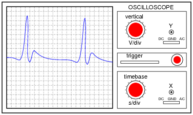
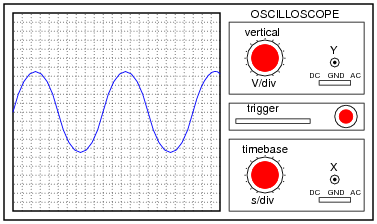
The basic oscilloscope, as shown in the illustration, is typically divided into four sections: the display, vertical controls, horizontal controls and trigger controls. The display is usually a CRT or LCD panel which is laid out with both horizontal and vertical reference lines referred to as the graticule. In addition to the screen, most display sections are equipped with three basic controls: a focus knob, an intensity knob and a beam finder button.The vertical section controls the amplitude of the displayed signal. This section carries a Volts-per-Division (Volts/Div) selector knob, an AC/DC/Ground selector switch and the vertical (primary) input for the instrument. Additionally, this section is typically equipped with the vertical beam position knob.
The horizontal section controls the time base or "sweep" of the instrument. The primary control is the Seconds-per-Division (Sec/Div) selector switch. Also included is a horizontal input for plotting dual X-Y axis signals. The horizontal beam position knob is generally located in this section.
The trigger section controls the start event of the sweep. The trigger can be set to automatically restart after each sweep or it can be configured to respond to an internal or external event. The principal controls of this section will be the source and coupling selector switches. An external trigger input (EXT Input) and level adjustment will also be included.
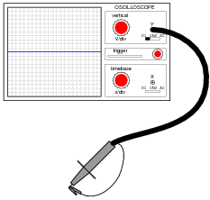
In addition to the basic instrument, most oscilloscopes are supplied with a probe as shown. The probe will connect to any input on the instrument and typically has a resistor of ten times the oscilloscope's input impedance. This results in a .1 (‑10X) attenuation factor, but helps to isolate the capacitive load presented by the probe cable from the signal being measured. Some probes have a switch allowing the operator to bypass the resistor when appropriate.
Size and portability
Most modern oscilloscopes are lightweight, portable instruments that are compact enough to be easily carried by a single person. In addition to the portable units, the market offers a number of miniature battery-powered instruments for field service applications. Laboratory grade oscilloscopes, especially older units which use vacuum tubes, are generally bench-top devices or may be mounted into dedicated carts. Special-purpose oscilloscopes may be rack-mounted or permanently mounted into a custom instrument housing.Inputs
The signal to be measured is fed to one of the input connectors, which is usually a coaxial connector such as a BNC or UHF type. Binding posts or banana plugs may be used for lower frequencies. If the signal source has its own coaxial connector, then a simple coaxial cable is used; otherwise, a specialized cable called a "scope probe", supplied with the oscilloscope, is used. In general, for routine use, an open wire test lead for connecting to the point being observed is not satisfactory, and a probe is generally necessary. General-purpose oscilloscopes usually present an input impedance of 1 megohm in parallel with a small but known capacitance such as 20 picofarads.[4] This allows the use of standard oscilloscope probes.[5] Scopes for use with very high frequencies may have 50‑ohm inputs, which must be either connected directly to a 50‑ohm signal source or used with Z0 or active probes.Less-frequently-used inputs include one (or two) for triggering the sweep, horizontal deflection for X‑Y mode displays, and trace brightening/darkening, sometimes called z'‑axis inputs.
Probes
Open wire test leads (flying leads) are likely to pick up interference, so they are not suitable for low level signals. Furthermore, the leads have a high inductance, so they are not suitable for high frequencies. Using a shielded cable (i.e., coaxial cable) is better for low level signals. Coaxial cable also has lower inductance, but it has higher capacitance: a typical 50 ohm cable has about 90 pF per meter. Consequently, a one-meter direct (1X) coaxial probe will load a circuit with a capacitance of about 110 pF and a resistance of 1 megohm.To minimize loading, attenuator probes (e.g., 10X probes) are used. A typical probe uses a 9 megohm series resistor shunted by a low-value capacitor to make an RC compensated divider with the cable capacitance and scope input. The RC time constants are adjusted to match. For example, the 9 megohm series resistor is shunted by a 12.2 pF capacitor for a time constant of 110 microseconds. The cable capacitance of 90 pF in parallel with the scope input of 20 pF and 1 megohm (total capacitance 110 pF) also gives a time constant of 110 microseconds. In practice, there will be an adjustment so the operator can precisely match the low frequency time constant (called compensating the probe). Matching the time constants makes the attenuation independent of frequency. At low frequencies (where the resistance of R is much less than the reactance of C), the circuit looks like a resistive divider; at high frequencies (resistance much greater than reactance), the circuit looks like a capacitive divider.
The result is a frequency compensated probe for modest frequencies that presents a load of about 10 megohms shunted by 12 pF. Although such a probe is an improvement, it does not work when the time scale shrinks to several cable transit times (transit time is typically 5 ns). In that time frame, the cable looks like its characteristic impedance, and there will be reflections from the transmission line mismatch at the scope input and the probe that causes ringing.[7] The modern scope probe uses lossy low capacitance transmission lines and sophisticated frequency shaping networks to make the 10X probe perform well at several hundred megahertz. Consequently, there are other adjustments for completing the compensation.
Probes with 10:1 attenuation are by far the most common; for large signals (and slightly-less capacitive loading), 100:1 probes are not rare. There are also probes that contain switches to select 10:1 or direct (1:1) ratios, but one must be aware that the 1:1 setting has significant capacitance (tens of pF) at the probe tip, because the whole cable's capacitance is now directly connected.
Most oscilloscopes allow for probe attenuation factors, displaying the effective sensitivity at the probe tip. Historically, some auto-sensing circuitry used indicator lamps behind translucent windows in the panel to illuminate different parts of the sensitivity scale. To do so, the probe connectors (modified BNCs) had an extra contact to define the probe's attenuation. (A certain value of resistor, connected to ground, "encodes" the attenuation.) Because probes wear out, and because the auto-sensing circuitry is not compatible between different makes of oscilloscope, auto-sensing probe scaling is not foolproof. Likewise, manually setting the probe attenuation is prone to user error and it is a common mistake to have the probe scaling set incorrectly; resultant voltage readings can then be wrong by a factor of 10.
There are special high voltage probes which also form compensated attenuators with the oscilloscope input; the probe body is physically large, and some require partly filling a canister surrounding the series resistor with volatile liquid fluorocarbon to displace air. At the oscilloscope end is a box with several waveform-trimming adjustments. For safety, a barrier disc keeps one's fingers distant from the point being examined. Maximum voltage is in the low tens of kV. (Observing a high voltage ramp can create a staircase waveform with steps at different points every repetition, until the probe tip is in contact. Until then, a tiny arc charges the probe tip, and its capacitance holds the voltage (open circuit). As the voltage continues to climb, another tiny arc charges the tip further.)
There are also current probes, with cores that surround the conductor carrying current to be examined. One type has a hole for the conductor, and requires that the wire be passed through the hole; they are for semi-permanent or permanent mounting. However, other types, for testing, have a two-part core that permit them to be placed around a wire. Inside the probe, a coil wound around the core provides a current into an appropriate load, and the voltage across that load is proportional to current. However, this type of probe can sense AC, only.
A more-sophisticated probe includes a magnetic flux sensor (Hall effect sensor) in the magnetic circuit. The probe connects to an amplifier, which feeds (low frequency) current into the coil to cancel the sensed field; the magnitude of that current provides the low-frequency part of the current waveform, right down to DC. The coil still picks up high frequencies. There is a combining network akin to a loudspeaker crossover network.
Front panel controls
Focus control
This control adjusts CRT focus to obtain the sharpest, most-detailed trace. In practice, focus needs to be adjusted slightly when observing quite-different signals, which means that it needs to be an external control. Flat-panel displays do not need focus adjustments and therefore do not include this control.Intensity control
This adjusts trace brightness. Slow traces on CRT oscilloscopes need less, and fast ones, especially if not often repeated, require more. On flat panels, however, trace brightness is essentially independent of sweep speed, because the internal signal processing effectively synthesizes the display from the digitized data.Astigmatism
Can also be called "Shape" or "spot shape". Adjusts the relative voltages on two of the CRT anodes such that a displayed spot changes from elliptical in one plane through a circular spot to an ellipse at 90 degrees to the first. This control may be absent from simpler oscilloscope designs or may even be an internal control. It is not necessary with flat panel displays.Beam finder
Modern oscilloscopes have direct-coupled deflection amplifiers, which means the trace could be deflected off-screen. They also might have their beam blanked without the operator knowing it. To help in restoring a visible display, the beam finder circuit overrides any blanking and limits the beam deflected to the visible portion of the screen. Beam-finder circuits often distort the trace while activated.Graticule
The graticule is a grid of squares that serve as reference marks for measuring the displayed trace. These markings, whether located directly on the screen or on a removable plastic filter, usually consist of a 1 cm grid with closer tick marks (often at 2 mm) on the centre vertical and horizontal axis. One expects to see ten major divisions across the screen; the number of vertical major divisions varies. Comparing the grid markings with the waveform permits one to measure both voltage (vertical axis) and time (horizontal axis). Frequency can also be determined by measuring the waveform period and calculating its reciprocal.On old and lower-cost CRT oscilloscopes the graticule is a sheet of plastic, often with light-diffusing markings and concealed lamps at the edge of the graticule. The lamps had a brightness control. Higher-cost instruments have the graticule marked on the inside face of the CRT, to eliminate parallax errors; better ones also had adjustable edge illumination with diffusing markings. (Diffusing markings appear bright.) Digital oscilloscopes, however, generate the graticule markings on the display in the same way as the trace.
External graticules also protect the glass face of the CRT from accidental impact. Some CRT oscilloscopes with internal graticules have an unmarked tinted sheet plastic light filter to enhance trace contrast; this also serves to protect the faceplate of the CRT.
Accuracy and resolution of measurements using a graticule is relatively limited; better instruments sometimes have movable bright markers on the trace that permit internal circuits to make more refined measurements.
Both calibrated vertical sensitivity and calibrated horizontal time are set in 1 - 2 - 5 - 10 steps. This leads, however, to some awkward interpretations of minor divisions
Timebase controls
These select the horizontal speed of the CRT's spot as it creates the trace; this process is commonly referred to as the sweep. In all but the least-costly modern oscilloscopes, the sweep speed is selectable and calibrated in units of time per major graticule division. Quite a wide range of sweep speeds is generally provided, from seconds to as fast as picoseconds (in the fastest) per division. Usually, a continuously-variable control (often a knob in front of the calibrated selector knob) offers uncalibrated speeds, typically slower than calibrated. This control provides a range somewhat greater than that of consecutive calibrated steps, making any speed available between the extremes.
Holdoff control
Found on some better analog oscilloscopes, this varies the time (holdoff) during which the sweep circuit ignores triggers. It provides a stable display of some repetitive events in which some triggers would create confusing displays. It is usually set to minimum, because a longer time decreases the number of sweeps per second, resulting in a dimmer trace.Vertical sensitivity, coupling, and polarity controls
To accommodate a wide range of input amplitudes, a switch selects calibrated sensitivity of the vertical deflection. Another control, often in front of the calibrated-selector knob, offers a continuously-variable sensitivity over a limited range from calibrated to less-sensitive settings.Often the observed signal is offset by a steady component, and only the changes are of interest. A switch (AC position) connects a capacitor in series with the input that passes only the changes (provided that they are not too slow -- "slow" would mean visible). However, when the signal has a fixed offset of interest, or changes quite slowly, the input is connected directly (DC switch position). Most oscilloscopes offer the DC input option. For convenience, to see where zero volts input currently shows on the screen, many oscilloscopes have a third switch position (GND) that disconnects the input and grounds it. Often, in this case, the user centers the trace with the Vertical Position control.
Better oscilloscopes have a polarity selector. Normally, a positive input moves the trace upward, but this permits inverting—positive deflects the trace downward.
Horizontal sensitivity control
This control is found only on more elaborate oscilloscopes; it offers adjustable sensitivity for external horizontal inputs.Vertical position control
The vertical position control moves the whole displayed trace up and down. It is used to set the no-input trace exactly on the center line of the graticule, but also permits offsetting vertically by a limited amount. With direct coupling, adjustment of this control can compensate for a limited DC component of an input.
Horizontal position control
The horizontal position control moves the display sidewise. It usually sets the left end of the trace at the left edge of the graticule, but it can displace the whole trace when desired. This control also moves the X-Y mode traces sidewise in some instruments, and can compensate for a limited DC component as for vertical position.
Dual-trace controls
Each input channel usually has its own set of sensitivity, coupling, and position controls, although some four-trace oscilloscopes have only minimal controls for their third and fourth channels.
Dual-trace oscilloscopes have a mode switch to select either channel alone, both channels, or (in some) an X‑Y display, which uses the second channel for X deflection. When both channels are displayed, the type of channel switching can be selected on some oscilloscopes; on others, the type depends upon timebase setting. If manually selectable, channel switching can be free-running (asynchronous), or between consecutive sweeps. Some Philips dual-trace analog oscilloscopes had a fast analog multiplier, and provided a display of the product of the input channels.
Multiple-trace oscilloscopes have a switch for each channel to enable or disable display of that trace's signal.
Delayed-sweep controls
These include controls for the delayed-sweep timebase, which is calibrated, and often also variable. The slowest speed is several steps faster than the slowest main sweep speed, although the fastest is generally the same. A calibrated multiturn delay time control offers wide range, high resolution delay settings; it spans the full duration of the main sweep, and its reading corresponds to graticule divisions (but with much finer precision). Its accuracy is also superior to that of the display.A switch selects display modes: Main sweep only, with a brightened region showing when the delayed sweep is advancing, delayed sweep only, or (on some) a combination mode.
Good CRT oscilloscopes include a delayed-sweep intensity control, to allow for the dimmer trace of a much-faster delayed sweep that nevertheless occurs only once per main sweep. Such oscilloscopes also are likely to have a trace separation control for multiplexed display of both the main and delayed sweeps together.
Sweep trigger controls
A switch selects the Trigger Source. It can be an external input, one of the vertical channels of a dual or multiple-trace oscilloscope, or the AC line (mains) frequency. Another switch enables or disables Auto trigger mode, or selects single sweep, if provided in the oscilloscope. Either a spring-return switch position or a pushbutton arms single sweeps.
A Level control varies the voltage on the waveform which generates a trigger, and the Slope switch selects positive-going or negative-going polarity at the selected trigger level.
Basic types of sweep
Triggered sweep

Type 465 Tektronix oscilloscope. This was a popular analog oscilloscope, portable, and is a representative example.
A triggered sweep starts at a selected point on the signal, providing a stable display. In this way, triggering allows the display of periodic signals such as sine waves and square waves, as well as nonperiodic signals such as single pulses, or pulses that do not recur at a fixed rate.
With triggered sweeps, the scope will blank the beam and start to reset the sweep circuit each time the beam reaches the extreme right side of the screen. For a period of time, called holdoff, (extendable by a front-panel control on some better oscilloscopes), the sweep circuit resets completely and ignores triggers. Once holdoff expires, the next trigger starts a sweep. The trigger event is usually the input waveform reaching some user-specified threshold voltage (trigger level) in the specified direction (going positive or going negative—trigger polarity).
In some cases, variable holdoff time can be really useful to make the sweep ignore interfering triggers that occur before the events to be observed. In the case of repetitive, but complex waveforms, variable holdoff can create a stable display that cannot otherwise be achieved.
Holdoff
Trigger holdoff defines a certain period following a trigger during which the scope will not trigger again. This makes it easier to establish a stable view of a waveform with multiple edges which would otherwise cause another trigger.Example
Imagine the following repeating waveform:
The green line is the waveform, the red vertical partial line represents the location of the trigger, and the yellow line represents the trigger level. If the scope was simply set to trigger on every rising edge, this waveform would cause three triggers for each cycle:


Assuming the signal is fairly high frequency, the scope would probably look something like this:

Except that on the scope, each trigger would be the same channel, and so would be the same color.
It is desired to set the scope to only trigger on one edge per cycle, so it is necessary to set the holdoff to be slightly less than the period of the waveform. That will prevent it from triggering more than once per cycle, but still allow it to trigger on the first edge of the next cycle.
Automatic sweep mode
Triggered sweeps can display a blank screen if there are no triggers. To avoid this, these sweeps include a timing circuit that generates free-running triggers so a trace is always visible. Once triggers arrive, the timer stops providing pseudo-triggers. Automatic sweep mode can be de-selected when observing low repetition rates.Recurrent sweeps
If the input signal is periodic, the sweep repetition rate can be adjusted to display a few cycles of the waveform. Early (tube) oscilloscopes and lowest-cost oscilloscopes have sweep oscillators that run continuously, and are uncalibrated. Such oscilloscopes are very simple, comparatively inexpensive, and were useful in radio servicing and some TV servicing. Measuring voltage or time is possible, but only with extra equipment, and is quite inconvenient. They are primarily qualitative instruments.They have a few (widely spaced) frequency ranges, and relatively wide-range continuous frequency control within a given range. In use, the sweep frequency is set to slightly lower than some submultiple of the input frequency, to display typically at least two cycles of the input signal (so all details are visible). A very simple control feeds an adjustable amount of the vertical signal (or possibly, a related external signal) to the sweep oscillator. The signal triggers beam blanking and a sweep retrace sooner than it would occur free-running, and the display becomes stable.
Single sweeps
Some oscilloscopes offer these—the sweep circuit is manually armed (typically by a pushbutton or equivalent) "Armed" means it's ready to respond to a trigger. Once the sweep is complete, it resets, and will not sweep until re-armed. This mode, combined with an oscilloscope camera, captures single-shot events.Types of trigger include:
- external trigger, a pulse from an external source connected to a dedicated input on the scope.
- edge trigger, an edge-detector that generates a pulse when the input signal crosses a specified threshold voltage in a specified direction. These are the most-common types of triggers; the level control sets the threshold voltage, and the slope control selects the direction (negative or positive-going). (The first sentence of the description also applies to the inputs to some digital logic circuits; those inputs have fixed threshold and polarity response.)
- video trigger, a circuit that extracts synchronizing pulses from video formats such as PAL and NTSC and triggers the timebase on every line, a specified line, every field, or every frame. This circuit is typically found in a waveform monitor device, although some better oscilloscopes include this function.
- delayed trigger, which waits a specified time after an edge trigger before starting the sweep. As described under delayed sweeps, a trigger delay circuit (typically the main sweep) extends this delay to a known and adjustable interval. In this way, the operator can examine a particular pulse in a long train of pulses.
Delayed sweeps
More sophisticated analog oscilloscopes contain a second timebase for a delayed sweep. A delayed sweep provides a very detailed look at some small selected portion of the main timebase. The main timebase serves as a controllable delay, after which the delayed timebase starts. This can start when the delay expires, or can be triggered (only) after the delay expires. Ordinarily, the delayed timebase is set for a faster sweep, sometimes much faster, such as 1000:1. At extreme ratios, jitter in the delays on consecutive main sweeps degrades the display, but delayed-sweep triggers can overcome that.The display shows the vertical signal in one of several modes: the main timebase, or the delayed timebase only, or a combination thereof. When the delayed sweep is active, the main sweep trace brightens while the delayed sweep is advancing. In one combination mode, provided only on some oscilloscopes, the trace changes from the main sweep to the delayed sweep once the delayed sweep starts, although less of the delayed fast sweep is visible for longer delays. Another combination mode multiplexes (alternates) the main and delayed sweeps so that both appear at once; a trace separation control displaces them.
DSOs allow waveforms to be displayed in this way, without offering a delayed timebase as such.
Dual and multiple-trace oscilloscopes
Oscilloscopes with two vertical inputs, referred to as dual-trace oscilloscopes, are extremely useful and commonplace. Using a single-beam CRT, they multiplex the inputs, usually switching between them fast enough to display two traces apparently at once. Less common are oscilloscopes with more traces; four inputs are common among these, but a few (Kikusui, for one) offered a display of the sweep trigger signal if desired. Some multi-trace oscilloscopes use the external trigger input as an optional vertical input, and some have third and fourth channels with only minimal controls. In all cases, the inputs, when independently displayed, are time-multiplexed, but dual-trace oscilloscopes often can add their inputs to display a real-time analog sum. (Inverting one channel provides a difference, provided that neither channel is overloaded. This difference mode can provide a moderate-performance differential input.)Switching channels can be asynchronous, that is, free-running, with trace blanking while switching, or after each horizontal sweep is complete. Asynchronous switching is usually designated "Chopped", while sweep-synchronized is designated "Alt[ernate]". A given channel is alternately connected and disconnected, leading to the term "chopped". Multi-trace oscilloscopes also switch channels either in chopped or alternate modes.
In general, chopped mode is better for slower sweeps. It is possible for the internal chopping rate to be a multiple of the sweep repetition rate, creating blanks in the traces, but in practice this is rarely a problem; the gaps in one trace are overwritten by traces of the following sweep. A few oscilloscopes had a modulated chopping rate to avoid this occasional problem. Alternate mode, however, is better for faster sweeps.
True dual-beam CRT oscilloscopes did exist, but were not common. One type (Cossor, U.K.) had a beam-splitter plate in its CRT, and single-ended deflection following the splitter. Others had two complete electron guns, requiring tight control of axial (rotational) mechanical alignment in manufacturing the CRT. Beam-splitter types had horizontal deflection common to both vertical channels, but dual-gun oscilloscopes could have separate time bases, or use one time base for both channels. Multiple-gun CRTs (up to ten guns) were made in past decades. With ten guns, the envelope (bulb) was cylindrical throughout its length.
The vertical amplifier
In an analog oscilloscope, the vertical amplifier acquires the signal[s] to be displayed. In better oscilloscopes, it delays them by a fraction of a microsecond, and provides a signal large enough to deflect the CRT's beam. That deflection is at least somewhat beyond the edges of the graticule, and more typically some distance off-screen. The amplifier has to have low distortion to display its input accurately (it must be linear), and it has to recover quickly from overloads. As well, its time-domain response has to represent transients accurately—minimal overshoot, rounding, and tilt of a flat pulse top.A vertical input goes to a frequency-compensated step attenuator to reduce large signals to prevent overload. The attenuator feeds a low-level stage (or a few), which in turn feed gain stages (and a delay-line driver if there is a delay). Following are more gain stages, up to the final output stage which develops a large signal swing (tens of volts, sometimes over 100 volts) for CRT electrostatic deflection.
In dual and multiple-trace oscilloscopes, an internal electronic switch selects the relatively low-level output of one channel's amplifiers and sends it to the following stages of the vertical amplifier, which is only a single channel, so to speak, from that point on.
In free-running ("chopped") mode, the oscillator (which may be simply a different operating mode of the switch driver) blanks the beam before switching, and unblanks it only after the switching transients have settled.
Part way through the amplifier is a feed to the sweep trigger circuits, for internal triggering from the signal. This feed would be from an individual channel's amplifier in a dual or multi-trace oscilloscope, the channel depending upon the setting of the trigger source selector.
This feed precedes the delay (if there is one), which allows the sweep circuit to unblank the CRT and start the forward sweep, so the CRT can show the triggering event. High-quality analog delays add a modest cost to an oscilloscope, and are omitted in oscilloscopes that are cost-sensitive.
The delay, itself, comes from a special cable with a pair of conductors wound around a flexible, magnetically soft core. The coiling provides distributed inductance, while a conductive layer close to the wires provides distributed capacitance. The combination is a wideband transmission line with considerable delay per unit length. Both ends of the delay cable require matched impedances to avoid reflections.
X-Y mode

A 24-hour clock displayed on a CRT oscilloscope configured in X-Y mode as a vector monitor with dual R2R DACs to generate the analog voltages.
The X-Y mode also allows the oscilloscope to be used as a vector monitor to display images or user interfaces. Many early games, such as Tennis for Two, used an oscilloscope as an output device.
Complete loss of signal in an X-Y CRT display means that the beam strikes a small spot, which risks burning the phosphor. Older phosphors burned more easily. Some dedicated X-Y displays reduce beam current greatly, or blank the display entirely, if there are no inputs present.
Bandwidth
As with all practical instruments, oscilloscopes do not respond equally to all possible input frequencies. The range of frequencies an oscilloscope can usefully display is referred to as its bandwidth. Bandwidth applies primarily to the Y-axis, although the X-axis sweeps have to be fast enough to show the highest-frequency waveforms.The bandwidth is defined as the frequency at which the sensitivity is 0.707 of that at DC or the lowest AC frequency (a drop of 3 dB). The oscilloscope's response will drop off rapidly as the input frequency is raised above that point. Within the stated bandwidth the response will not necessarily be exactly uniform (or "flat"), but should always fall within a +0 to -3 dB range. One source[12] states that there is a noticeable effect on the accuracy of voltage measurements at only 20 percent of the stated bandwidth. Some oscilloscopes' specifications do include a narrower tolerance range within the stated bandwidth.
Probes also have bandwidth limits and must be chosen and used to properly handle the frequencies of interest. To achieve the flattest response, most probes must be "compensated" (an adjustment performed using a test signal from the oscilloscope) to allow for the reactance of the probe's cable.
Another related specification is rise time. This is the duration of the fastest pulse that can be resolved by the scope. It is related to the bandwidth approximately by:
Bandwidth in Hz x rise time in seconds = 0.35
For example, an oscilloscope intended to resolve pulses with a rise time of 1 nanosecond would have a bandwidth of 350 MHz.
In analog instruments, the bandwidth of the oscilloscope is limited by the vertical amplifiers and the CRT or other display subsystem. In digital instruments, the sampling rate of the analog to digital converter (ADC) is a factor, but the stated analog bandwidth (and therefore the overall bandwidth of the instrument) is usually less than the ADC's Nyquist frequency. This is due to limitations in the analog signal amplifier, deliberate design of the Anti-aliasing filter that precedes the ADC, or both.
For a digital oscilloscope, a rule of thumb is that the continuous sampling rate should be ten times the highest frequency desired to resolve; for example a 20 megasample/second rate would be applicable for measuring signals up to about 2 megahertz. This allows the anti-aliasing filter to be designed with a 3 dB down point of 2 MHz and an effective cutoff at 10 MHz (the Nyquist frequency), avoiding the artifacts of a very steep ("brick-wall") filter.
A sampling oscilloscope can display signals of considerably higher frequency than the sampling rate if the signals are exactly, or nearly, repetitive. It does this by taking one sample from each successive repetition of the input waveform, each sample being at an increased time interval from the trigger event. The waveform is then displayed from these collected samples. This mechanism is referred to as "equivalent-time sampling".Some oscilloscopes can operate in either this mode or in the more traditional "real-time" mode at the operator's choice.
Other features
Some oscilloscopes have cursors, which are lines that can be moved about the screen to measure the time interval between two points, or the difference between two voltages. A few older oscilloscopes simply brightened the trace at movable locations. These cursors are more accurate than visual estimates referring to graticule lines.
Better quality general purpose oscilloscopes include a calibration signal for setting up the compensation of test probes; this is (often) a 1 kHz square-wave signal of a definite peak-to-peak voltage available at a test terminal on the front panel. Some better oscilloscopes also have a squared-off loop for checking and adjusting current probes.
Sometimes the event that the user wants to see may only happen occasionally. To catch these events, some oscilloscopes, known as "storage scopes", preserve the most recent sweep on the screen. This was originally achieved by using a special CRT, a "storage tube", which would retain the image of even a very brief event for a long time.
Some digital oscilloscopes can sweep at speeds as slow as once per hour, emulating a strip chart recorder. That is, the signal scrolls across the screen from right to left. Most oscilloscopes with this facility switch from a sweep to a strip-chart mode at about one sweep per ten seconds. This is because otherwise, the scope looks broken: it's collecting data, but the dot cannot be seen.
In current oscilloscopes, digital signal sampling is more often used for all but the simplest models. Samples feed fast analog-to-digital converters, following which all signal processing (and storage) is digital.
Many oscilloscopes have different plug-in modules for different purposes, e.g., high-sensitivity amplifiers of relatively narrow bandwidth, differential amplifiers, amplifiers with four or more channels, sampling plugins for repetitive signals of very high frequency, and special-purpose plugins, including audio/ultrasonic spectrum analyzers, and stable-offset-voltage direct-coupled channels with relatively high gain.
Examples of use
.gif)
Lissajous figures on an oscilloscope, with 90 degrees phase difference between x and y inputs.
In a piece of electronic equipment, for example, the connections between stages (e.g. electronic mixers, electronic oscillators, amplifiers) may be 'probed' for the expected signal, using the scope as a simple signal tracer. If the expected signal is absent or incorrect, some preceding stage of the electronics is not operating correctly. Since most failures occur because of a single faulty component, each measurement can prove that half of the stages of a complex piece of equipment either work, or probably did not cause the fault.
Once the faulty stage is found, further probing can usually tell a skilled technician exactly which component has failed. Once the component is replaced, the unit can be restored to service, or at least the next fault can be isolated. This sort of troubleshooting is typical of radio and TV receivers, as well as audio amplifiers, but can apply to quite-different devices such as electronic motor drives.
Another use is to check newly designed circuitry. Very often a newly designed circuit will misbehave because of design errors, bad voltage levels, electrical noise etc. Digital electronics usually operate from a clock, so a dual-trace scope which shows both the clock signal and a test signal dependent upon the clock is useful. Storage scopes are helpful for "capturing" rare electronic events that cause defective operation.
Automotive use
First appearing in the 1970s for ignition system analysis, automotive oscilloscopes are becoming an important workshop tool for testing sensors and output signals on electronic engine management systems, braking and stability systems. Some oscilloscopes can trigger and decode serial bus messages, such as the CAN bus commonly used in automotive applications.Selection
For work at high frequencies and with fast digital signals, the bandwidth of the vertical amplifiers and sampling rate must be high enough. For general-purpose use, a bandwidth of at least 100 MHz is usually satisfactory. A much lower bandwidth is sufficient for audio-frequency applications only. A useful sweep range is from one second to 100 nanoseconds, with appropriate triggering and (for analog instruments) sweep delay. A well-designed, stable trigger circuit is required for a steady display. The chief benefit of a quality oscilloscope is the quality of the trigger circuit.Key selection criteria of a DSO (apart from input bandwidth) are the sample memory depth and sample rate. Early DSOs in the mid- to late 1990s only had a few KB of sample memory per channel. This is adequate for basic waveform display, but does not allow detailed examination of the waveform or inspection of long data packets for example. Even entry-level (<$500) modern DSOs now have 1 MB or more of sample memory per channel, and this has become the expected minimum in any modern DSO. Often this sample memory is shared between channels, and can sometimes only be fully available at lower sample rates. At the highest sample rates, the memory may be limited to a few tens of KB.[15] Any modern "real-time" sample rate DSO will have typically 5–10 times the input bandwidth in sample rate. So a 100 MHz bandwidth DSO would have 500 Ms/s – 1 Gs/s sample rate. The theoretical minimum sample rate required, using SinX/x interpolation, is 2.5 times the bandwidth.[16]
Analog oscilloscopes have been almost totally displaced by digital storage scopes except for use exclusively at lower frequencies. Greatly increased sample rates have largely eliminated the display of incorrect signals, known as "aliasing", that was sometimes present in the first generation of digital scopes. The problem can still occur when, for example, viewing a short section of a repetitive waveform that repeats at intervals thousands of times longer than the section viewed (for example a short synchronization pulse at the beginning of a particular television line), with an oscilloscope that cannot store the extremely large number of samples between one instance of the short section and the next.
The used test equipment market, particularly on-line auction venues, typically has a wide selection of older analog scopes available. However it is becoming more difficult to obtain replacement parts for these instruments, and repair services are generally unavailable from the original manufacturer. Used instruments are usually out of calibration, and recalibration by companies with the equipment and expertise usually costs more than the second-hand value of the instrument.
As of 2007[update], a 350 MHz bandwidth (BW), 2.5 gigasamples per second (GS/s), dual-channel digital storage scope costs about US$7000 new.
On the lowest end, an inexpensive hobby-grade single-channel DSO could be purchased for under $90 as of June 2011. These often have limited bandwidth and other facilities, but fulfill the basic functions of an oscilloscope.
Software
Many oscilloscopes today provide one or more external interfaces to allow remote instrument control by external software. These interfaces (or buses) include GPIB, Ethernet, serial port, and USB.Types and models
The following section is a brief summary of various types and models available. For a detailed discussion, refer to the other article.Cathode-ray oscilloscope (CRO)
.jpg)

For analog television, an analog oscilloscope can be used as a vectorscope to analyze complex signal properties, such as this display of SMPTE color bars.
Analog scopes do not necessarily include a calibrated reference grid for size measurement of waves, and they may not display waves in the traditional sense of a line segment sweeping from left to right. Instead, they could be used for signal analysis by feeding a reference signal into one axis and the signal to measure into the other axis. For an oscillating reference and measurement signal, this results in a complex looping pattern referred to as a Lissajous curve. The shape of the curve can be interpreted to identify properties of the measurement signal in relation to the reference signal, and is useful across a wide range of oscillation frequencies.
Dual-beam oscilloscope
The dual-beam analog oscilloscope can display two signals simultaneously. A special dual-beam CRT generates and deflects two separate beams. Although multi-trace analog oscilloscopes can simulate a dual-beam display with chop and alternate sweeps, those features do not provide simultaneous displays. (Real time digital oscilloscopes offer the same benefits of a dual-beam oscilloscope, but they do not require a dual-beam display.) The disadvantages of the dual trace oscilloscope are that it cannot switch quickly between the traces and it cannot capture two fast transient events. In order to avoid this problems a dual beam oscilloscope is used.Analog storage oscilloscope
Trace storage is an extra feature available on some analog scopes; they used direct-view storage CRTs. Storage allows the trace pattern that normally decays in a fraction of a second to remain on the screen for several minutes or longer. An electrical circuit can then be deliberately activated to store and erase the trace on the screen.Digital oscilloscopes
While analog devices make use of continually varying voltages, digital devices employ binary numbers which correspond to samples of the voltage. In the case of digital oscilloscopes, an analog-to-digital converter (ADC) is used to change the measured voltages into digital information.The digital storage oscilloscope, or DSO for short, is now the preferred type for most industrial applications, although simple analog CROs are still used by hobbyists. It replaces the electrostatic storage method used in analog storage scopes with digital memory, which can store data as long as required without degradation and with uniform brightness. It also allows complex processing of the signal by high-speed digital signal processing circuits.[3]

A standard DSO is limited to capturing signals with a bandwidth of less than half the sampling rate of the ADC (called the Nyquist limit). There is a variation of the DSO called the digital sampling oscilloscope that can exceed this limit for certain types of signal, such as high-speed communications signals, where the waveform consists of repeating pulses. This type of DSO deliberately samples at a much lower frequency than the Nyquist limit and then uses signal processing to reconstruct a composite view of a typical pulse. A similar technique, with analog rather than digital samples, was used before the digital era in analog sampling oscilloscopes.
A digital phosphor oscilloscope (DPO) uses color information to convey information about a signal. It may, for example, display infrequent signal data in blue to make it stand out. In a conventional analog scope, such a rare trace may not be visible.
Mixed-signal oscilloscopes
A mixed-signal oscilloscope (or MSO) has two kinds of inputs, a small number of analog channels (typically two or four), and a larger number of digital channels(typically sixteen). It provides the ability to accurately time-correlate analog and digital channels, thus offering a distinct advantage over a separate oscilloscope and logic analyser. Typically, digital channels may be grouped and displayed as a bus with each bus value displayed at the bottom of the display in hex or binary. On most MSOs, the trigger can be set across both analog and digital channels.Mixed-domain oscilloscopes
In a mixed-domain oscilloscope (MDO) you have an additional RF input port that goes into a spectrum analyzer part. It links those traditionally separate instruments, so that you can e.g. time correlate events in the time domain (like a specific serial data package) with events happening in the frequency domain (like RF transmissions).Handheld oscilloscopes
Handheld oscilloscopes are useful for many test and field service applications. Today, a hand held oscilloscope is usually a digital sampling oscilloscope, using a liquid crystal display.
Many hand-held and bench oscilloscopes have the ground reference voltage common to all input channels. If more than one measurement channel is used at the same time, all the input signals must have the same voltage reference, and the shared default reference is the "earth". If there is no differential preamplifier or external signal isolator, this traditional desktop oscilloscope is not suitable for floating measurements. (Occasionally an oscilloscope user will break the ground pin in the power supply cord of a bench-top oscilloscope in an attempt to isolate the signal common from the earth ground. This practice is unreliable since the entire stray capacitance of the instrument cabinet will be connected into the circuit. Since it is also a hazard to break a safety ground connection, instruction manuals strongly advise against this practice.)
Some models of oscilloscope have isolated inputs, where the signal reference level terminals are not connected together. Each input channel can be used to make a "floating" measurement with an independent signal reference level. Measurements can be made without tying one side of the oscilloscope input to the circuit signal common or ground reference.

The isolation available is categorized as shown below:
| Overvoltage category | Operating voltage (effective value of AC/DC to ground) | Peak instantaneous voltage (repeated 20 times) | Test resistor |
|---|---|---|---|
| CAT I | 600 V | 2500 V | 30 Ω |
| CAT I | 1000 V | 4000 V | 30 Ω |
| CAT II | 600 V | 4000 V | 12 Ω |
| CAT II | 1000 V | 6000 V | 12 Ω |
| CAT III | 600 V | 6000 V | 2 Ω |
PC-based oscilloscopes
A new type of oscilloscope is emerging that consists of a specialized signal acquisition board (which can be an external USB or parallel port device, or an internal add-on PCI or ISA card). The user interface and signal processing software runs on the user's computer, rather than on an embedded computer as in the case of a conventional DSO.
Related instruments
A large number of instruments used in a variety of technical fields are really oscilloscopes with inputs, calibration, controls, display calibration, etc., specialized and optimized for a particular application. Examples of such oscilloscope-based instruments include waveform monitors for analyzing video levels in television productions and medical devices such as vital function monitors and electrocardiogram and electroencephalogram instruments. In automobile repair, an ignition analyzer is used to show the spark waveforms for each cylinder. All of these are essentially oscilloscopes, performing the basic task of showing the changes in one or more input signals over time in an X‑Y display.Other instruments convert the results of their measurements to a repetitive electrical signal, and incorporate an oscilloscope as a display element. Such complex measurement systems include spectrum analyzers, transistor analyzers, and time domain reflectometers (TDRs). Unlike an oscilloscope, these instruments automatically generate stimulus or sweep a measurement parameter.
conjunction Networking and the Internet to biggest oscilloscope minus sequence

Visualization of a portion of the routes on the Internet
In time, the network spread beyond academic and military institutions and became known as the Internet. The emergence of networking involved a redefinition of the nature and boundaries of the computer. Computer operating systems and applications were modified to include the ability to define and access the resources of other computers on the network, such as peripheral devices, stored information, and the like, as extensions of the resources of an individual computer. Initially these facilities were available primarily to people working in high-tech environments, but in the 1990s the spread of applications like e-mail and the World Wide Web, combined with the development of cheap, fast networking technologies like Ethernet and ADSL saw computer networking become almost ubiquitous. In fact, the number of computers that are networked is growing phenomenally. A very large proportion of personal computers regularly connect to the Internet to communicate and receive information. "Wireless" networking, often utilizing mobile phone networks, has meant networking is becoming increasingly ubiquitous even in mobile computing environments
There is active research to make computers out of many promising new types of technology, such as optical computers, DNA computers, neural computers, and quantum computers. Most computers are universal, and are able to calculate any computable function, and are limited only by their memory capacity and operating speed. However different designs of computers can give very different performance for particular problems; for example quantum computers can potentially break some modern encryption algorithms (by quantum factoring) very quickly.
Computer architecture paradigms
- Quantum computer vs. Chemical computer
- Scalar processor vs. Vector processor
- Non-Uniform Memory Access (NUMA) computers
- Register machine vs. Stack machine
- Harvard architecture vs. von Neumann architecture
- Cellular architecture
Artificial intelligence
A computer will solve problems in exactly the way it is programmed to, without regard to efficiency, alternative solutions, possible shortcuts, or possible errors in the code. Computer programs that learn and adapt are part of the emerging field of artificial intelligence and machine learning.Basic Oscilloscope Operation
AC Electric Circuits
Question 1
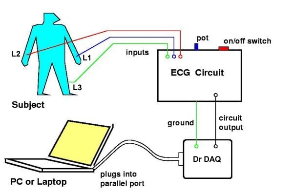
An oscilloscope is a very useful piece of electronic test equipment. Most everyone has seen an oscilloscope in use, in the form of a heart-rate monitor (electrocardiogram, or EKG) of the type seen in doctor’s offices and hospitals.
When monitoring heart beats, what do the two axes (horizontal and vertical) of the oscilloscope screen represent?
In general electronics use, when measuring AC voltage signals, what do the two axes (horizontal and vertical) of the oscilloscope screen represent?

When monitoring heart beats, what do the two axes (horizontal and vertical) of the oscilloscope screen represent?
Question 2
The core of an analog oscilloscope is a special type of vacuum tube known as a Cathode Ray Tube, or CRT. While similar in function to the CRT used in televisions, oscilloscope display tubes are specially built for the purpose of serving an a measuring instrument.
Explain how a CRT functions. What goes on inside the tube to produce waveform displays on the screen?
Explain how a CRT functions. What goes on inside the tube to produce waveform displays on the screen?
Question 3
Question 4
Question 5
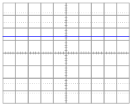
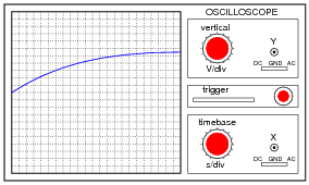
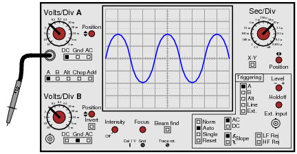
A technician prepares to use an oscilloscope to display an AC voltage signal. After turning the oscilloscope on and connecting the Y input probe to the signal source test points, this display appears:
What display control(s) need to be adjusted on the oscilloscope in order to show fewer cycles of this signal on the screen, with a greater height (amplitude)?
Question 6
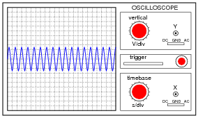
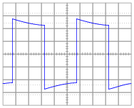
A technician prepares to use an oscilloscope to display an AC voltage signal. After turning the oscilloscope on and connecting the Y input probe to the signal source test points, this display appears:
What display control(s) need to be adjusted on the oscilloscope in order to show a normal-looking wave on the screen?
Question 7
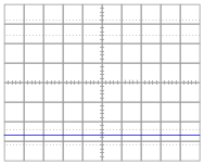
A technician prepares to use an oscilloscope to display an AC voltage signal. After turning the oscilloscope on and connecting the Y input probe to the signal source test points, this display appears:
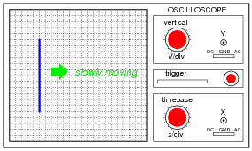
What appears on the oscilloscope screen is a vertical line that moves slowly from left to right. What display control(s) need to be adjusted on the oscilloscope in order to show a normal-looking wave on the screen?
Question 8
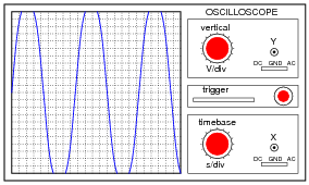
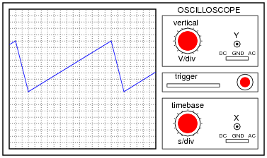
A technician prepares to use an oscilloscope to display an AC voltage signal. After turning the oscilloscope on and connecting the Y input probe to the signal source test points, this display appears:
What display control(s) need to be adjusted on the oscilloscope in order to show a normal-looking wave on the screen?
Question 9
Question 10
Question 11
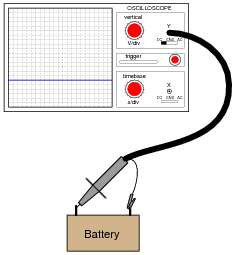
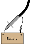
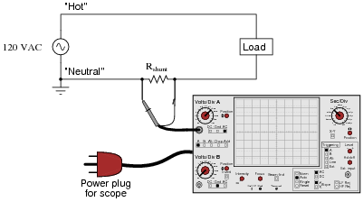
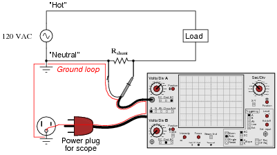
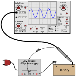
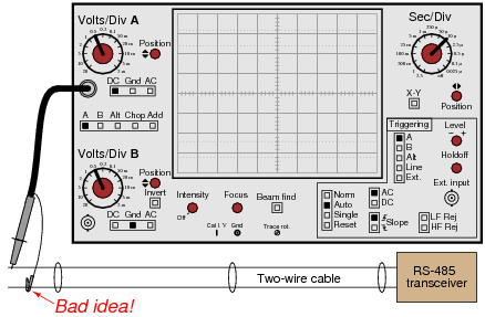
Most oscilloscopes can only directly measure voltage, not current. One way to measure AC current with an oscilloscope is to measure the voltage dropped across a shunt resistor. Since the voltage dropped across a resistor is proportional to the current through that resistor, whatever wave-shape the current is will be translated into a voltage drop with the exact same wave-shape.
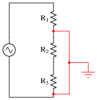
However, one must be very careful when connecting an oscilloscope to any part of a grounded system, as many electric power systems are. Note what happens here when a technician attempts to connect the oscilloscope across a shunt resistor located on the “hot” side of a grounded 120 VAC motor circuit:
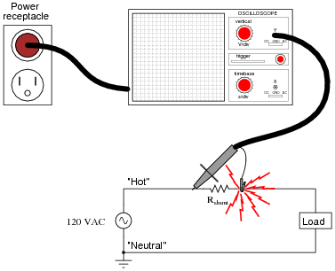
Here, the reference lead of the oscilloscope (the small alligator clip, not the sharp-tipped probe) creates a short-circuit in the power system. Explain why this happens.
However, one must be very careful when connecting an oscilloscope to any part of a grounded system, as many electric power systems are. Note what happens here when a technician attempts to connect the oscilloscope across a shunt resistor located on the “hot” side of a grounded 120 VAC motor circuit:
Question 12
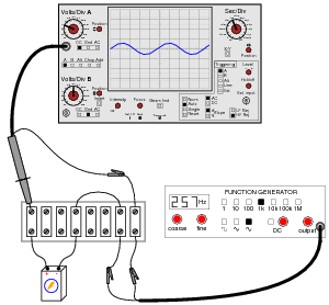
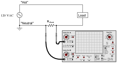
Most oscilloscopes have at least two vertical inputs, used to display more than one waveform simultaneously:
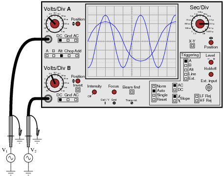
While this feature is extremely useful, one must be careful in connecting two sources of AC voltage to an oscilloscope. Since the “reference” or “ground” clips of each probe are electrically common with the oscilloscope’s metal chassis, they are electrically common with each other as well.
Explain what sort of problem would be caused by connecting a dual-trace oscilloscope to a circuit in the following manner:
Explain what sort of problem would be caused by connecting a dual-trace oscilloscope to a circuit in the following manner:
Question 13
Question 14
Question 15

Question 16
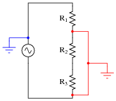
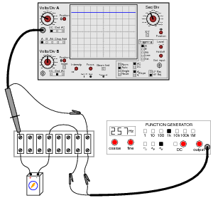
Shunt resistors are low-value, precision resistors used as current-measuring elements in high-current circuits. The idea is to measure the voltage dropped across this precision resistance and use Ohm’s Law (I = V/R) to infer the amount of current in the circuit:

Since the schematic shows a shunt resistor being used to measure current in an AC circuit, it would be equally appropriate to use an oscilloscope instead of a voltmeter to measure the voltage drop produced by the shunt. However, we must be careful in connecting the oscilloscope to the shunt because of the inherent ground reference of the oscilloscope’s metal case and probe assembly.
Explain why connecting an oscilloscope to the shunt as shown in this second diagram would be a bad idea:
Explain why connecting an oscilloscope to the shunt as shown in this second diagram would be a bad idea:
Question 17
Question 18
One of the more complicated controls to master on an oscilloscope, but also one of the most useful, is the triggering control. Without proper “triggering,” a waveform will scroll horizontally across the screen rather than staying “locked” in place.
Describe how the triggering control is able to “lock” an AC waveform on the screen so that it appears stable to the human eye. What, exactly, is the triggering function doing that makes an AC waveform appear to stand still?
Describe how the triggering control is able to “lock” an AC waveform on the screen so that it appears stable to the human eye. What, exactly, is the triggering function doing that makes an AC waveform appear to stand still?
Question 19
If an oscilloscope is connected to a series combination of AC and DC voltage sources, what is displayed on the oscilloscope screen depends on where the “coupling” control is set.
With the coupling control set to “DC”, the waveform displayed will be elevated above (or depressed below) the “zero” line:
Setting the coupling control to ÄC”, however, results in the waveform automatically centering itself on the screen, about the zero line.
Based on these observations, explain what the “DC” and ÄC” settings on the coupling control actually mean.
With the coupling control set to “DC”, the waveform displayed will be elevated above (or depressed below) the “zero” line:
Question 20

Question 21
Suppose a technician measures the voltage output by an AC-DC power supply circuit:
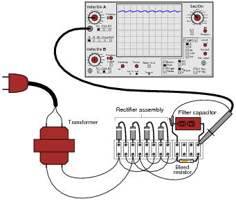
The waveform shown by the oscilloscope is mostly DC, with just a little bit of AC “ripple” voltage appearing as a ripple pattern on what would otherwise be a straight, horizontal line. This is quite normal for the output of an AC-DC power supply.
Suppose we wished to take a closer view of this “ripple” voltage. We want to make the ripples more pronounced on the screen, so that we may better discern their shape. Unfortunately, though, when we decrease the number of volts per division on the “vertical” control knob to magnify the vertical amplification of the oscilloscope, the pattern completely disappears from the screen!
Explain what the problem is, and how we might correct it so as to be able to magnify the ripple voltage waveform without having it disappear off the oscilloscope screen.
Question 22
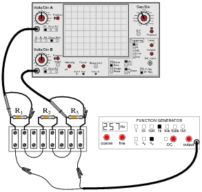
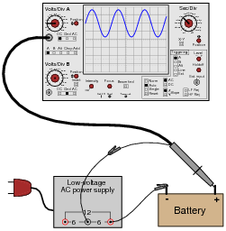
A student just learning to use oscilloscopes connects one directly to the output of a signal generator, with these results:
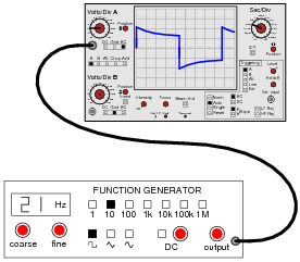
As you can see, the function generator is configured to output a square wave, but the oscilloscope does not register a square wave. Perplexed, the student takes the function generator to a different oscilloscope. At the second oscilloscope, the student sees a proper square wave on the screen:
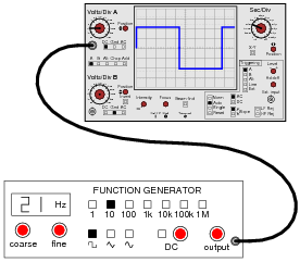
It is then that the student realizes the first oscilloscope has its “coupling” control set to AC, while the second oscilloscope was set to DC. Now the student is really confused! The signal is obviously AC, as it oscillates above and below the centerline of the screen, but yet the “DC” setting appears to give the most accurate results: a true-to-form square wave.
How would you explain what is happening to this student, and also describe the appropriate uses of the ÄC” and “DC” coupling settings so he or she knows better how to use it in the future?
How would you explain what is happening to this student, and also describe the appropriate uses of the ÄC” and “DC” coupling settings so he or she knows better how to use it in the future?
Question 23
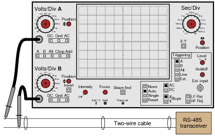
There are times when you need to use an oscilloscope to measure a differential voltage that also has a significant common-mode voltage: an application where you cannot connect the oscilloscope’s ground lead to either point of contact. One application is measuring the voltage pulses on an RS-485 digital communications network, where neither conductor in the two-wire cable is at ground potential, and where connecting either wire to ground (via the oscilloscope’s ground clip) may cause problems:
One solution to this problem is to use both probes of a dual-trace oscilloscope, and set it up for differential measurement. In this mode, only one waveform will be shown on the screen, even though two probes are being used. No ground clips need be connected to the circuit under test, and the waveform shown will be indicative of the voltage between the two probe tips.
Describe how a typical oscilloscope may be set up to perform differential voltage measurement. Be sure to include descriptions of all knob and button settings (with reference to the oscilloscope shown in this question):
Describe how a typical oscilloscope may be set up to perform differential voltage measurement. Be sure to include descriptions of all knob and button settings (with reference to the oscilloscope shown in this question):

Question 24
A very common accessory for oscilloscopes is a ×10 probe, which effectively acts as a 10:1 voltage divider for any measured signals. Thus, an oscilloscope showing a waveform with a peak-to-peak amplitude of 4 divisions, with a vertical sensitivity setting of 1 volt per division, using a ×10 probe, would actually be measuring a signal of 40 volts peak-peak:
Obviously, one use for a ×10 probe is measuring voltages beyond the normal range of an oscilloscope. However, there is another application that is less obvious, and it regards the input impedance of the oscilloscope. A ×10 probe gives the oscilloscope 10 times more input impedance (as seen from the probe tip to ground). Typically this means an input impedance of 10 MΩ (with the ×10 probe) rather than 1 MΩ (with a normal 1:1 probe). Identify an application where this feature could be useful.
I won’t give away an answer here, but I will provide a hint in the form of another question: why is it generally a good thing for voltmeters to have high input impedance? Or conversely, what bad things might happen if you tried to use a low-impedance voltmeter to measure voltages?
Notes:
Increased input impedance is often a more common reason for choosing ×10 probes, as opposed to increased voltage measurement range. The answer to this question is more readily grasped by students after they have worked with loading-sensitive electronic circuits
Increased input impedance is often a more common reason for choosing ×10 probes, as opposed to increased voltage measurement range. The answer to this question is more readily grasped by students after they have worked with loading-sensitive electronic circuits

Pulse computation
Pulse computation is a hybrid of digital and analog computation that uses aperiodic electrical spikes, as opposed to the periodic voltages in a digital computer or the continuously varying voltages in an analog computer. Pulse streams are unlocked, so they can arrive at arbitrary times and can be generated by analog processes, although each spike is allocated a binary value, as it would be in a digital computer.
Pulse computation is primarily studied as part of the field of neural networks. The processing unit in such a network is called a "neuron".


A computer network or data network is a digital telecommunications network which allows nodes to share resources. In computer networks, networked computing devices exchange data with each other using a data link. The connections between nodes are established using either cable media or wireless media.
Network computer devices that originate, route and terminate the data are called network nodes.[1] Nodes can include hosts such as personal computers, phones, servers as well as networking hardware. Two such devices can be said to be networked together when one device is able to exchange information with the other device, whether or not they have a direct connection to each other. In most cases, application-specific communications protocols are layered (i.e. carried as payload) over other more general communications protocols. This formidable collection of information technology requires skilled network management to keep it all running reliably.
Computer networks support an enormous number of applications and services such as access to the World Wide Web, digital video, digital audio, shared use of application and storage servers, printers, and fax machines, and use of email and instant messaging applications as well as many others. Computer networks differ in the transmission medium used to carry their signals, communications protocols to organize network traffic, the network's size, topology and organizational intent. The best-known computer network is the Internet.
Computer networking may be considered a branch of electrical engineering, telecommunications, computer science, information technology or computer engineering, since it relies upon the theoretical and practical application of the related disciplines.
A computer network facilitates interpersonal communications allowing users to communicate efficiently and easily via various means: email, instant messaging, online chat, telephone, video telephone calls, and video conferencing. A network allows sharing of network and computing resources. Users may access and use resources provided by devices on the network, such as printing a document on a shared network printer or use of a shared storage device. A network allows sharing of files, data, and other types of information giving authorized users the ability to access information stored on other computers on the network. Distributed computing uses computing resources across a network to accomplish tasks.
A computer network may be used by security hackers to deploy computer viruses or computer worms on devices connected to the network, or to prevent these devices from accessing the network via a denial-of-service attack.
Computer communication links that do not support packets, such as traditional point-to-point telecommunication links, simply transmit data as a bit stream. However, most information in computer networks is carried in packets. A network packet is a formatted unit of data (a list of bits or bytes, usually a few tens of bytes to a few kilobytes long) carried by a packet-switched network.
In packet networks, the data is formatted into packets that are sent through the network to their destination. Once the packets arrive they are reassembled into their original message. With packets, the bandwidth of the transmission medium can be better shared among users than if the network were circuit switched. When one user is not sending packets, the link can be filled with packets from other users, and so the cost can be shared, with relatively little interference, provided the link isn't overused.
Packets consist of two kinds of data: control information, and user data (payload). The control information provides data the network needs to deliver the user data, for example: source and destination network addresses, error detection codes, and sequencing information. Typically, control information is found in packet headers and trailers, with payload data in between.
Often the route a packet needs to take through a network is not immediately available. In that case the packet is queued and waits until a link is free.
A widely adopted family of transmission media used in local area network (LAN) technology is collectively known as Ethernet. The media and protocol standards that enable communication between networked devices over Ethernet are defined by IEEE 802.3. Ethernet transmits data over both copper and fiber cables. Wireless LAN standards (e.g. those defined by IEEE 802.11) use radio waves, or others use infrared signals as a transmission medium. Power line communication uses a building's power cabling to transmit data.
 The orders of the following wired technologies are, roughly, from slowest to fastest transmission speed.
 A network interface controller (NIC) is computer hardware that provides a computer with the ability to access the transmission media, and has the ability to process low-level network information. For example, the NIC may have a connector for accepting a cable, or an aerial for wireless transmission and reception, and the associated circuitry.
The NIC responds to traffic addressed to a network address for either the NIC or the computer as a whole.
In Ethernet networks, each network interface controller has a unique Media Access Control (MAC) address—usually stored in the controller's permanent memory. To avoid address conflicts between network devices, the Institute of Electrical and Electronics Engineers (IEEE) maintains and administers MAC address uniqueness. The size of an Ethernet MAC address is six octets. The three most significant octets are reserved to identify NIC manufacturers. These manufacturers, using only their assigned prefixes, uniquely assign the three least-significant octets of every Ethernet interface they produce.
A repeater with multiple ports is known as a hub. Repeaters work on the physical layer of the OSI model. Repeaters require a small amount of time to regenerate the signal. This can cause a propagation delay that affects network performance and may affect proper function. As a result, many network architectures limit the number of repeaters that can be used in a row, e.g., the Ethernet 5-4-3 rule.
Hubs and repeaters in LANs have been mostly obsoleted by modern switches.
Bridges come in three basic types:
Multi-layer switches are capable of routing based on layer 3 addressing or additional logical levels. The term switch is often used loosely to include devices such as routers and bridges, as well as devices that may distribute traffic based on load or based on application content (e.g., a Web URL identifier).
A router is an internetworking device that forwards packets between networks by processing the routing information included in the packet or datagram (Internet protocol information from layer 3). The routing information is often processed in conjunction with the routing table (or forwarding table). A router uses its routing table to determine where to forward packets. A destination in a routing table can include a "null" interface, also known as the "black hole" interface because data can go into it, however, no further processing is done for said data, i.e. the packets are dropped.
Overlay networks have been around since the invention of networking when computer systems were connected over telephone lines using modems, before any data network existed.
The most striking example of an overlay network is the Internet itself. The Internet itself was initially built as an overlay on the telephone network.[11] Even today, each Internet node can communicate with virtually any other through an underlying mesh of sub-networks of wildly different topologies and technologies. Address resolution and routing are the means that allow mapping of a fully connected IP overlay network to its underlying network.
Another example of an overlay network is a distributed hash table, which maps keys to nodes in the network. In this case, the underlying network is an IP network, and the overlay network is a table (actually a map) indexed by keys.
Overlay networks have also been proposed as a way to improve Internet routing, such as through quality of service guarantees to achieve higher-quality streaming media. Previous proposals such as IntServ, DiffServ, and IP Multicast have not seen wide acceptance largely because they require modification of all routers in the network.[citation needed] On the other hand, an overlay network can be incrementally deployed on end-hosts running the overlay protocol software, without cooperation from Internet service providers. The overlay network has no control over how packets are routed in the underlying network between two overlay nodes, but it can control, for example, the sequence of overlay nodes that a message traverses before it reaches its destination.
For example, Akamai Technologies manages an overlay network that provides reliable, efficient content delivery (a kind of multicast). Academic research includes end system multicast,[12] resilient routing and quality of service studies, among others.
A communications protocol is a set of rules for exchanging information over a network. In a protocol stack (also see the OSI model), each protocol leverages the services of the protocol below it. An important example of a protocol stack is HTTP (the World Wide Web protocol) running over TCP over IP (the Internet protocols) over IEEE 802.11 (the Wi-Fi protocol). This stack is used between the wireless router and the home user's personal computer when the user is surfing the web.
While the use of protocol layering is today ubiquitous across the field of computer networking, it has been historically criticized by many researchers[13] for two principal reasons. Firstly, abstracting the protocol stack in this way may cause a higher layer to duplicate functionality of a lower layer, a prime example being error recovery on both a per-link basis and an end-to-end basis.[14] Secondly, it is common that a protocol implementation at one layer may require data, state or addressing information that is only present at another layer, thus defeating the point of separating the layers in the first place. For example, TCP uses the ECN field in the IPv4 header as an indication of congestion; IP is a network layer protocol whereas TCP is a transport layer protocol.
Communication protocols have various characteristics. They may be connection-oriented or connectionless, they may use circuit mode or packet switching, and they may use hierarchical addressing or flat addressing.
There are many communication protocols, a few of which are described below.
For example, MAC bridging (IEEE 802.1D) deals with the routing of Ethernet packets using a Spanning Tree Protocol. IEEE 802.1Q describes VLANs, and IEEE 802.1X defines a port-based Network Access Control protocol, which forms the basis for the authentication mechanisms used in VLANs (but it is also found in WLANs) – it is what the home user sees when the user has to enter a "wireless access key".
While the role of ATM is diminishing in favor of next-generation networks, it still plays a role in the last mile, which is the connection between an Internet service provider and the home user.[15]
A network can be characterized by its physical capacity or its organizational purpose. Use of the network, including user authorization and access rights, differ accordingly.
The defining characteristics of a LAN, in contrast to a wide area network (WAN), include higher data transfer rates, limited geographic range, and lack of reliance on leased lines to provide connectivity. Current Ethernet or other IEEE 802.3 LAN technologies operate at data transfer rates up to 100 Gbit/s, standarized by IEEE in 2010.[20] Currently, 400 Gbit/s Ethernet is being developed.
A LAN can be connected to a WAN using a router.
For example, a university campus network is likely to link a variety of campus buildings to connect academic colleges or departments, the library, and student residence halls.
For example, a large company might implement a backbone network to connect departments that are located around the world. The equipment that ties together the departmental networks constitutes the network backbone. When designing a network backbone, network performance and network congestion are critical factors to take into account. Normally, the backbone network's capacity is greater than that of the individual networks connected to it.
Another example of a backbone network is the Internet backbone, which is the set of wide area networks (WANs) and core routers that tie together all networks connected to the Internet.
VPN may have best-effort performance, or may have a defined service level agreement (SLA) between the VPN customer and the VPN service provider. Generally, a VPN has a topology more complex than point-to-point.
 The Internet is the largest example of an internetwork. It is a global system of interconnected governmental, academic, corporate, public, and private computer networks. It is based on the networking technologies of the Internet Protocol Suite. It is the successor of the Advanced Research Projects Agency Network (ARPANET) developed by DARPA of the United States Department of Defense. The Internet is also the communications backbone underlying the World Wide Web (WWW).
Participants in the Internet use a diverse array of methods of several hundred documented, and often standardized, protocols compatible with the Internet Protocol Suite and an addressing system (IP addresses) administered by the Internet Assigned Numbers Authority and address registries. Service providers and large enterprises exchange information about the reachability of their address spaces through the Border Gateway Protocol (BGP), forming a redundant worldwide mesh of transmission paths.
Darknets are distinct from other distributed peer-to-peer networks as sharing is anonymous (that is, IP addresses are not publicly shared), and therefore users can communicate with little fear of governmental or corporate interference.[23]
Routing is the process of selecting network paths to carry network traffic. Routing is performed for many kinds of networks, including circuit switching networks and packet switched networks.
In packet switched networks, routing directs packet forwarding (the transit of logically addressed network packets from their source toward their ultimate destination) through intermediate nodes. Intermediate nodes are typically network hardware devices such as routers, bridges, gateways, firewalls, or switches. General-purpose computers can also forward packets and perform routing, though they are not specialized hardware and may suffer from limited performance. The routing process usually directs forwarding on the basis of routing tables, which maintain a record of the routes to various network destinations. Thus, constructing routing tables, which are held in the router's memory, is very important for efficient routing.
There are usually multiple routes that can be taken, and to choose between them, different elements can be considered to decide which routes get installed into the routing table, such as (sorted by priority):
Routing, in a more narrow sense of the term, is often contrasted with bridging in its assumption that network addresses are structured and that similar addresses imply proximity within the network. Structured addresses allow a single routing table entry to represent the route to a group of devices. In large networks, structured addressing (routing, in the narrow sense) outperforms unstructured addressing (bridging). Routing has become the dominant form of addressing on the Internet. Bridging is still widely used within localized environments.
The World Wide Web, E-mail,[24] printing and network file sharing are examples of well-known network services. Network services such as DNS (Domain Name System) give names for IP and MAC addresses (people remember names like “nm.lan” better than numbers like “210.121.67.18”),[25] and DHCP to ensure that the equipment on the network has a valid IP address.[26]
Services are usually based on a service protocol that defines the format and sequencing of messages between clients and servers of that network service.
The following list gives examples of network performance measures for a circuit-switched network and one type of packet-switched network, viz. ATM:
Network protocols that use aggressive retransmissions to compensate for packet loss tend to keep systems in a state of network congestion—even after the initial load is reduced to a level that would not normally induce network congestion. Thus, networks using these protocols can exhibit two stable states under the same level of load. The stable state with low throughput is known as congestive collapse.
Modern networks use congestion control and congestion avoidance techniques to try to avoid congestion collapse. These include: exponential backoff in protocols such as 802.11's CSMA/CA and the original Ethernet, window reduction in TCP, and fair queueing in devices such as routers. Another method to avoid the negative effects of network congestion is implementing priority schemes, so that some packets are transmitted with higher priority than others. Priority schemes do not solve network congestion by themselves, but they help to alleviate the effects of congestion for some services. An example of this is 802.1p. A third method to avoid network congestion is the explicit allocation of network resources to specific flows. One example of this is the use of Contention-Free Transmission Opportunities (CFTXOPs) in the ITU-T G.hn standard, which provides high-speed (up to 1 Gbit/s) Local area networking over existing home wires (power lines, phone lines and coaxial cables).
For the Internet RFC 2914 addresses the subject of congestion control in detail.
Computer and network surveillance programs are widespread today, and almost all Internet traffic is or could potentially be monitored for clues to illegal activity.
Surveillance is very useful to governments and law enforcement to maintain social control, recognize and monitor threats, and prevent/investigate criminal activity. With the advent of programs such as the Total Information Awareness program, technologies such as high speed surveillance computers and biometrics software, and laws such as the Communications Assistance For Law Enforcement Act, governments now possess an unprecedented ability to monitor the activities of citizens.[32]
However, many civil rights and privacy groups—such as Reporters Without Borders, the Electronic Frontier Foundation, and the American Civil Liberties Union—have expressed concern that increasing surveillance of citizens may lead to a mass surveillance society, with limited political and personal freedoms. Fears such as this have led to numerous lawsuits such as Hepting v. AT&T.[32][33] The hacktivist group Anonymous has hacked into government websites in protest of what it considers "draconian surveillance".[34][35]
Examples of end-to-end encryption include PGP for email, OTR for instant messaging, ZRTP for telephony, and TETRA for radio.
Typical server-based communications systems do not include end-to-end encryption. These systems can only guarantee protection of communications between clients and servers, not between the communicating parties themselves. Examples of non-E2EE systems are Google Talk, Yahoo Messenger, Facebook, and Dropbox. Some such systems, for example LavaBit and SecretInk, have even described themselves as offering "end-to-end" encryption when they do not. Some systems that normally offer end-to-end encryption have turned out to contain a back door that subverts negotiation of the encryption key between the communicating parties, for example Skype or Hushmail.
The end-to-end encryption paradigm does not directly address risks at the communications endpoints themselves, such as the technical exploitation of clients, poor quality random number generators, or key escrow. E2EE also does not address traffic analysis, which relates to things such as the identities of the end points and the times and quantities of messages that are sent.
Network administrators can see networks from both physical and logical perspectives. The physical perspective involves geographic locations, physical cabling, and the network elements (e.g., routers, bridges and application layer gateways) that interconnect via the transmission media. Logical networks, called, in the TCP/IP architecture, subnets, map onto one or more transmission media. For example, a common practice in a campus of buildings is to make a set of LAN cables in each building appear to be a common subnet, using virtual LAN (VLAN) technology.
Both users and administrators are aware, to varying extents, of the trust and scope characteristics of a network. Again using TCP/IP architectural terminology, an intranet is a community of interest under private administration usually by an enterprise, and is only accessible by authorized users (e.g. employees).[36] Intranets do not have to be connected to the Internet, but generally have a limited connection. An extranet is an extension of an intranet that allows secure communications to users outside of the intranet (e.g. business partners, customers).[36]
Unofficially, the Internet is the set of users, enterprises, and content providers that are interconnected by Internet Service Providers (ISP). From an engineering viewpoint, the Internet is the set of subnets, and aggregates of subnets, which share the registered IP address space and exchange information about the reachability of those IP addresses using the Border Gateway Protocol. Typically, the human-readable names of servers are translated to IP addresses, transparently to users, via the directory function of the Domain Name System (DNS).
Over the Internet, there can be business-to-business (B2B), business-to-consumer (B2C) and consumer-to-consumer (C2C) communications. When money or sensitive information is exchanged, the communications are apt to be protected by some form of communications security mechanism. Intranets and extranets can be securely superimposed onto the Internet, without any access by general Internet users and administrators, using secure Virtual Private Network (VPN) technology.
comparison computation with science
Systems science, systemology (greco. σύστημα - systema, λόγος - logos) or systems theory is an interdisciplinary field that studies the nature of systems — from simple to complex — in nature, society, cognition, and science itself. The field aims to develop interdisciplinary foundations that are applicable in a variety of areas, such as psychology, biology, medicine, communication, business management, engineering, and social sciences.[1]
Systems science covers formal sciences such as complex systems, cybernetics, dynamical systems theory, information theory, linguistics or systems theory. It has applications in the field of the natural and social sciences and engineering, such as control theory, operations research, social systems theory, systems biology, system dynamics, human factors, systems ecology, systems engineering and systems psychology.[2] Themes commonly stressed in system science are (a) holistic view, (b) interaction between a system and its embedding environment, and (c) complex (often subtle) trajectories of dynamic behavior that sometimes are stable (and thus reinforcing), while at various 'boundary conditions' can become wildly unstable (and thus destructive). Concerns about Earth-scale biosphere/geosphere dynamics is an example of the nature of problems to which systems science seeks to contribute meaningful insights.
Since the emergence of general systems research in the 1950s,[3] systems thinking and systems science have developed into many theoretical frameworks.

Among them were other scientists like Ackoff, Ashby, Margaret Mead and Churchman, who popularized the systems concept in the 1950s and 1960s. These scientists inspired and educated a second generation with more notable scientists like Ervin Laszlo (1932) and Fritjof Capra (1939), who wrote about systems theory in the 1970s and 1980s. Others got acquainted and started studying these works in the 1980s and started writing about it since the 1990s. Debora Hammond can be seen as a typical representative of these third generation of general systems scientists.
In the field of systems science the International Federation for Systems Research (IFSR) is an international federation for global and local societies in the field of systems science. This federation is a non-profit, scientific and educational agency founded in 1981, and constituted of some thirty member organizations from various countries. The overall purpose of this Federation is to advance cybernetic and systems research and systems applications and to serve the international systems community.
The best known research institute in the field is the Santa Fe Institute (SFI) located in Santa Fe, New Mexico, United States, dedicated to the study of complex systems. This institute was founded in 1984 by George Cowan, David Pines, Stirling Colgate, Murray Gell-Mann, Nick Metropolis, Herb Anderson, Peter A. Carruthers, and Richard Slansky. All but Pines and Gell-Mann were scientists with Los Alamos National Laboratory. SFI's original mission was to disseminate the notion of a separate interdisciplinary research area, complexity theory referred to at SFI as complexity science.
Pulse computation is primarily studied as part of the field of neural networks. The processing unit in such a network is called a "neuron".

A computer network or data network is a digital telecommunications network which allows nodes to share resources. In computer networks, networked computing devices exchange data with each other using a data link. The connections between nodes are established using either cable media or wireless media.
Network computer devices that originate, route and terminate the data are called network nodes.[1] Nodes can include hosts such as personal computers, phones, servers as well as networking hardware. Two such devices can be said to be networked together when one device is able to exchange information with the other device, whether or not they have a direct connection to each other. In most cases, application-specific communications protocols are layered (i.e. carried as payload) over other more general communications protocols. This formidable collection of information technology requires skilled network management to keep it all running reliably.
Computer networks support an enormous number of applications and services such as access to the World Wide Web, digital video, digital audio, shared use of application and storage servers, printers, and fax machines, and use of email and instant messaging applications as well as many others. Computer networks differ in the transmission medium used to carry their signals, communications protocols to organize network traffic, the network's size, topology and organizational intent. The best-known computer network is the Internet.
Computer networking may be considered a branch of electrical engineering, telecommunications, computer science, information technology or computer engineering, since it relies upon the theoretical and practical application of the related disciplines.
A computer network facilitates interpersonal communications allowing users to communicate efficiently and easily via various means: email, instant messaging, online chat, telephone, video telephone calls, and video conferencing. A network allows sharing of network and computing resources. Users may access and use resources provided by devices on the network, such as printing a document on a shared network printer or use of a shared storage device. A network allows sharing of files, data, and other types of information giving authorized users the ability to access information stored on other computers on the network. Distributed computing uses computing resources across a network to accomplish tasks.
A computer network may be used by security hackers to deploy computer viruses or computer worms on devices connected to the network, or to prevent these devices from accessing the network via a denial-of-service attack.
Computer communication links that do not support packets, such as traditional point-to-point telecommunication links, simply transmit data as a bit stream. However, most information in computer networks is carried in packets. A network packet is a formatted unit of data (a list of bits or bytes, usually a few tens of bytes to a few kilobytes long) carried by a packet-switched network.
In packet networks, the data is formatted into packets that are sent through the network to their destination. Once the packets arrive they are reassembled into their original message. With packets, the bandwidth of the transmission medium can be better shared among users than if the network were circuit switched. When one user is not sending packets, the link can be filled with packets from other users, and so the cost can be shared, with relatively little interference, provided the link isn't overused.
Packets consist of two kinds of data: control information, and user data (payload). The control information provides data the network needs to deliver the user data, for example: source and destination network addresses, error detection codes, and sequencing information. Typically, control information is found in packet headers and trailers, with payload data in between.
Often the route a packet needs to take through a network is not immediately available. In that case the packet is queued and waits until a link is free.
Network topology
The physical layout of a network is usually less important than the topology that connects network nodes. Most diagrams that describe a physical network are therefore topological, rather than geographic. The symbols on these diagrams usually denote network links and network nodes.Network links
The transmission media (often referred to in the literature as the physical media) used to link devices to form a computer network include electrical cable (Ethernet, HomePNA, power line communication, G.hn), optical fiber (fiber-optic communication), and radio waves (wireless networking). In the OSI model, these are defined at layers 1 and 2 — the physical layer and the data link layer.A widely adopted family of transmission media used in local area network (LAN) technology is collectively known as Ethernet. The media and protocol standards that enable communication between networked devices over Ethernet are defined by IEEE 802.3. Ethernet transmits data over both copper and fiber cables. Wireless LAN standards (e.g. those defined by IEEE 802.11) use radio waves, or others use infrared signals as a transmission medium. Power line communication uses a building's power cabling to transmit data.
Wired technologies

Fiber optic cables are used to transmit light from one computer/network node to another
- Coaxial cable is widely used for cable television systems, office buildings, and other work-sites for local area networks. The cables consist of copper or aluminum wire surrounded by an insulating layer (typically a flexible material with a high dielectric constant), which itself is surrounded by a conductive layer. The insulation helps minimize interference and distortion. Transmission speed ranges from 200 million bits per second to more than 500 million bits per second.
- ITU-T G.hn technology uses existing home wiring (coaxial cable, phone lines and power lines) to create a high-speed (up to 1 Gigabit/s) local area network
- Twisted pair wire is the most widely used medium for all telecommunication. Twisted-pair cabling consist of copper wires that are twisted into pairs. Ordinary telephone wires consist of two insulated copper wires twisted into pairs. Computer network cabling (wired Ethernet as defined by IEEE 802.3) consists of 4 pairs of copper cabling that can be utilized for both voice and data transmission. The use of two wires twisted together helps to reduce crosstalk and electromagnetic induction. The transmission speed ranges from 2 million bits per second to 10 billion bits per second. Twisted pair cabling comes in two forms: unshielded twisted pair (UTP) and shielded twisted-pair (STP). Each form comes in several category ratings, designed for use in various scenarios.

- An optical fiber is a glass fiber. It carries pulses of light that represent data. Some advantages of optical fibers over metal wires are very low transmission loss and immunity from electrical interference. Optical fibers can simultaneously carry multiple wavelengths of light, which greatly increases the rate that data can be sent, and helps enable data rates of up to trillions of bits per second. Optic fibers can be used for long runs of cable carrying very high data rates, and are used for undersea cables to interconnect continents.
Wireless technologies

- Terrestrial microwave – Terrestrial microwave communication uses Earth-based transmitters and receivers resembling satellite dishes. Terrestrial microwaves are in the low gigahertz range, which limits all communications to line-of-sight. Relay stations are spaced approximately 48 km (30 mi) apart.
- Communications satellites – Satellites communicate via microwave radio waves, which are not deflected by the Earth's atmosphere. The satellites are stationed in space, typically in geosynchronous orbit 35,400 km (22,000 mi) above the equator. These Earth-orbiting systems are capable of receiving and relaying voice, data, and TV signals.
- Cellular and PCS systems use several radio communications technologies. The systems divide the region covered into multiple geographic areas. Each area has a low-power transmitter or radio relay antenna device to relay calls from one area to the next area.
- Radio and spread spectrum technologies – Wireless local area networks use a high-frequency radio technology similar to digital cellular and a low-frequency radio technology. Wireless LANs use spread spectrum technology to enable communication between multiple devices in a limited area. IEEE 802.11 defines a common flavor of open-standards wireless radio-wave technology known as Wifi.
- Free-space optical communication uses visible or invisible light for communications. In most cases, line-of-sight propagation is used, which limits the physical positioning of communicating devices.
Exotic technologies
There have been various attempts at transporting data over exotic media:- IP over Avian Carriers was a humorous April fool's Request for Comments, issued as RFC 1149. It was implemented in real life in 2001.[7]
- Extending the Internet to interplanetary dimensions via radio waves, the Interplanetary Internet.[8]
Network nodes
Apart from any physical transmission media there may be, networks comprise additional basic system building blocks, such as network interface controllers (NICs), repeaters, hubs, bridges, switches, routers, modems, and firewalls. Any particular piece of equipment will frequently contain multiple building blocks and perform multiple functions.Network interfaces
.jpg)
An ATM network interface in the form of an accessory card. A lot of network interfaces are built-in.
The NIC responds to traffic addressed to a network address for either the NIC or the computer as a whole.
In Ethernet networks, each network interface controller has a unique Media Access Control (MAC) address—usually stored in the controller's permanent memory. To avoid address conflicts between network devices, the Institute of Electrical and Electronics Engineers (IEEE) maintains and administers MAC address uniqueness. The size of an Ethernet MAC address is six octets. The three most significant octets are reserved to identify NIC manufacturers. These manufacturers, using only their assigned prefixes, uniquely assign the three least-significant octets of every Ethernet interface they produce.
Repeaters and hubs[edit]
A repeater is an electronic device that receives a network signal, cleans it of unnecessary noise and regenerates it. The signal is retransmitted at a higher power level, or to the other side of an obstruction, so that the signal can cover longer distances without degradation. In most twisted pair Ethernet configurations, repeaters are required for cable that runs longer than 100 meters. With fiber optics, repeaters can be tens or even hundreds of kilometers apart.A repeater with multiple ports is known as a hub. Repeaters work on the physical layer of the OSI model. Repeaters require a small amount of time to regenerate the signal. This can cause a propagation delay that affects network performance and may affect proper function. As a result, many network architectures limit the number of repeaters that can be used in a row, e.g., the Ethernet 5-4-3 rule.
Hubs and repeaters in LANs have been mostly obsoleted by modern switches.
Bridges[edit]
A network bridge connects and filters traffic between two network segments at the data link layer (layer 2) of the OSI model to form a single network. This breaks the network's collision domain but maintains a unified broadcast domain. Network segmentation breaks down a large, congested network into an aggregation of smaller, more efficient networks.Bridges come in three basic types:
- Local bridges: Directly connect LANs
- Remote bridges: Can be used to create a wide area network (WAN) link between LANs. Remote bridges, where the connecting link is slower than the end networks, largely have been replaced with routers.
- Wireless bridges: Can be used to join LANs or connect remote devices to LANs.
Switches[edit]
A network switch is a device that forwards and filters OSI layer 2 datagrams (frames) between ports based on the destination MAC address in each frame.[9] A switch is distinct from a hub in that it only forwards the frames to the physical ports involved in the communication rather than all ports connected. It can be thought of as a multi-port bridge.[10] It learns to associate physical ports to MAC addresses by examining the source addresses of received frames. If an unknown destination is targeted, the switch broadcasts to all ports but the source. Switches normally have numerous ports, facilitating a star topology for devices, and cascading additional switches.Multi-layer switches are capable of routing based on layer 3 addressing or additional logical levels. The term switch is often used loosely to include devices such as routers and bridges, as well as devices that may distribute traffic based on load or based on application content (e.g., a Web URL identifier).
Routers[edit]

Modems
Modems (MOdulator-DEModulator) are used to connect network nodes via wire not originally designed for digital network traffic, or for wireless. To do this one or more carrier signals are modulated by the digital signal to produce an analog signal that can be tailored to give the required properties for transmission. Modems are commonly used for telephone lines, using a Digital Subscriber Line technology.Firewalls
A firewall is a network device for controlling network security and access rules. Firewalls are typically configured to reject access requests from unrecognized sources while allowing actions from recognized ones. The vital role firewalls play in network security grows in parallel with the constant increase in cyber attackss.Network structure
Network topology is the layout or organizational hierarchy of interconnected nodes of a computer network. Different network topologies can affect throughput, but reliability is often more critical. With many technologies, such as bus networks, a single failure can cause the network to fail entirely. In general the more interconnections there are, the more robust the network is; but the more expensive it is to install.Common layouts
Common layouts are:
- A bus network: all nodes are connected to a common medium along this medium. This was the layout used in the original Ethernet, called 10BASE5 and 10BASE2.
- A star network: all nodes are connected to a special central node. This is the typical layout found in a Wireless LAN, where each wireless client connects to the central Wireless access point.
- A ring network: each node is connected to its left and right neighbour node, such that all nodes are connected and that each node can reach each other node by traversing nodes left- or rightwards. The Fiber Distributed Data Interface (FDDI) made use of such a topology.
- A mesh network: each node is connected to an arbitrary number of neighbours in such a way that there is at least one traversal from any node to any other.
- A fully connected network: each node is connected to every other node in the network.
- A tree network: nodes are arranged hierarchically.
Overlay network
An overlay network is a virtual computer network that is built on top of another network. Nodes in the overlay network are connected by virtual or logical links. Each link corresponds to a path, perhaps through many physical links, in the underlying network. The topology of the overlay network may (and often does) differ from that of the underlying one. For example, many peer-to-peer networks are overlay networks. They are organized as nodes of a virtual system of links that run on top of the Internet.[11]
Overlay networks have been around since the invention of networking when computer systems were connected over telephone lines using modems, before any data network existed.
The most striking example of an overlay network is the Internet itself. The Internet itself was initially built as an overlay on the telephone network.[11] Even today, each Internet node can communicate with virtually any other through an underlying mesh of sub-networks of wildly different topologies and technologies. Address resolution and routing are the means that allow mapping of a fully connected IP overlay network to its underlying network.
Another example of an overlay network is a distributed hash table, which maps keys to nodes in the network. In this case, the underlying network is an IP network, and the overlay network is a table (actually a map) indexed by keys.
Overlay networks have also been proposed as a way to improve Internet routing, such as through quality of service guarantees to achieve higher-quality streaming media. Previous proposals such as IntServ, DiffServ, and IP Multicast have not seen wide acceptance largely because they require modification of all routers in the network.[citation needed] On the other hand, an overlay network can be incrementally deployed on end-hosts running the overlay protocol software, without cooperation from Internet service providers. The overlay network has no control over how packets are routed in the underlying network between two overlay nodes, but it can control, for example, the sequence of overlay nodes that a message traverses before it reaches its destination.
For example, Akamai Technologies manages an overlay network that provides reliable, efficient content delivery (a kind of multicast). Academic research includes end system multicast,[12] resilient routing and quality of service studies, among others.
Communications protocols


While the use of protocol layering is today ubiquitous across the field of computer networking, it has been historically criticized by many researchers[13] for two principal reasons. Firstly, abstracting the protocol stack in this way may cause a higher layer to duplicate functionality of a lower layer, a prime example being error recovery on both a per-link basis and an end-to-end basis.[14] Secondly, it is common that a protocol implementation at one layer may require data, state or addressing information that is only present at another layer, thus defeating the point of separating the layers in the first place. For example, TCP uses the ECN field in the IPv4 header as an indication of congestion; IP is a network layer protocol whereas TCP is a transport layer protocol.
Communication protocols have various characteristics. They may be connection-oriented or connectionless, they may use circuit mode or packet switching, and they may use hierarchical addressing or flat addressing.
There are many communication protocols, a few of which are described below.
IEEE 802
IEEE 802 is a family of IEEE standards dealing with local area networks and metropolitan area networks. The complete IEEE 802 protocol suite provides a diverse set of networking capabilities. The protocols have a flat addressing scheme. They operate mostly at levels 1 and 2 of the OSI model.For example, MAC bridging (IEEE 802.1D) deals with the routing of Ethernet packets using a Spanning Tree Protocol. IEEE 802.1Q describes VLANs, and IEEE 802.1X defines a port-based Network Access Control protocol, which forms the basis for the authentication mechanisms used in VLANs (but it is also found in WLANs) – it is what the home user sees when the user has to enter a "wireless access key".
Ethernet
Ethernet, sometimes simply called LAN, is a family of protocols used in wired LANs, described by a set of standards together called IEEE 802.3 published by the Institute of Electrical and Electronics Engineers.Wireless LAN
Wireless LAN, also widely known as WLAN or WiFi, is probably the most well-known member of the IEEE 802 protocol family for home users today. It is standarized by IEEE 802.11 and shares many properties with wired Ethernet.Internet Protocol Suite
The Internet Protocol Suite, also called TCP/IP, is the foundation of all modern networking. It offers connection-less as well as connection-oriented services over an inherently unreliable network traversed by data-gram transmission at the Internet protocol (IP) level. At its core, the protocol suite defines the addressing, identification, and routing specifications for Internet Protocol Version 4 (IPv4) and for IPv6, the next generation of the protocol with a much enlarged addressing capability.SONET/SD
Synchronous optical networking (SONET) and Synchronous Digital Hierarchy (SDH) are standardized multiplexing protocols that transfer multiple digital bit streams over optical fiber using lasers. They were originally designed to transport circuit mode communications from a variety of different sources, primarily to support real-time, uncompressed, circuit-switched voice encoded in PCM (Pulse-Code Modulation) format. However, due to its protocol neutrality and transport-oriented features, SONET/SDH also was the obvious choice for transporting Asynchronous Transfer Mode (ATM) frames.Asynchronous Transfer Mode
Asynchronous Transfer Mode (ATM) is a switching technique for telecommunication networks. It uses asynchronous time-division multiplexing and encodes data into small, fixed-sized cells. This differs from other protocols such as the Internet Protocol Suite or Ethernet that use variable sized packets or frames. ATM has similarity with both circuit and packet switched networking. This makes it a good choice for a network that must handle both traditional high-throughput data traffic, and real-time, low-latency content such as voice and video. ATM uses a connection-oriented model in which a virtual circuit must be established between two endpoints before the actual data exchange begins.While the role of ATM is diminishing in favor of next-generation networks, it still plays a role in the last mile, which is the connection between an Internet service provider and the home user.[15]
Cellular standards
There are a number of different digital cellular standards, including: Global System for Mobile Communications (GSM), General Packet Radio Service (GPRS), cdmaOne, CDMA2000, Evolution-Data Optimized (EV-DO), Enhanced Data Rates for GSM Evolution (EDGE), Universal Mobile Telecommunications System (UMTS), Digital Enhanced Cordless Telecommunications (DECT), Digital AMPS (IS-136/TDMA), and Integrated Digital Enhanced Network (iDEN).[16]Geographic scale
| Computer network types by spatial scope |
|---|
- Nanoscale network
- Personal area network
- Local area network
The defining characteristics of a LAN, in contrast to a wide area network (WAN), include higher data transfer rates, limited geographic range, and lack of reliance on leased lines to provide connectivity. Current Ethernet or other IEEE 802.3 LAN technologies operate at data transfer rates up to 100 Gbit/s, standarized by IEEE in 2010.[20] Currently, 400 Gbit/s Ethernet is being developed.
A LAN can be connected to a WAN using a router.
- Home area network
- Storage area network
- Campus area network
For example, a university campus network is likely to link a variety of campus buildings to connect academic colleges or departments, the library, and student residence halls.
- Backbone network
For example, a large company might implement a backbone network to connect departments that are located around the world. The equipment that ties together the departmental networks constitutes the network backbone. When designing a network backbone, network performance and network congestion are critical factors to take into account. Normally, the backbone network's capacity is greater than that of the individual networks connected to it.
Another example of a backbone network is the Internet backbone, which is the set of wide area networks (WANs) and core routers that tie together all networks connected to the Internet.
- Metropolitan area network
- Wide area network
- Enterprise private network
- Virtual private network
VPN may have best-effort performance, or may have a defined service level agreement (SLA) between the VPN customer and the VPN service provider. Generally, a VPN has a topology more complex than point-to-point.
- Global area network
Organizational scope
Networks are typically managed by the organizations that own them. Private enterprise networks may use a combination of intranets and extranets. They may also provide network access to the Internet, which has no single owner and permits virtually unlimited global connectivity.Intranet
An intranet is a set of networks that are under the control of a single administrative entity. The intranet uses the IP protocol and IP-based tools such as web browsers and file transfer applications. The administrative entity limits use of the intranet to its authorized users. Most commonly, an intranet is the internal LAN of an organization. A large intranet typically has at least one web server to provide users with organizational information. An intranet is also anything behind the router on a local area network.Extranet
An extranet is a network that is also under the administrative control of a single organization, but supports a limited connection to a specific external network. For example, an organization may provide access to some aspects of its intranet to share data with its business partners or customers. These other entities are not necessarily trusted from a security standpoint. Network connection to an extranet is often, but not always, implemented via WAN technology.Internetwork
An internetwork is the connection of multiple computer networks via a common routing technology using routers.Internet
Partial map of the Internet based on the January 15, 2005 data found on opte.org. Each line is drawn between two nodes, representing two IP addresses. The length of the lines are indicative of the delay between those two nodes. This graph represents less than 30% of the Class C networks reachable.
Participants in the Internet use a diverse array of methods of several hundred documented, and often standardized, protocols compatible with the Internet Protocol Suite and an addressing system (IP addresses) administered by the Internet Assigned Numbers Authority and address registries. Service providers and large enterprises exchange information about the reachability of their address spaces through the Border Gateway Protocol (BGP), forming a redundant worldwide mesh of transmission paths.
Darknet
A darknet is an overlay network, typically running on the internet, that is only accessible through specialized software. A darknet is an anonymizing network where connections are made only between trusted peers — sometimes called "friends" (F2F)[22] — using non-standard protocols and ports.Darknets are distinct from other distributed peer-to-peer networks as sharing is anonymous (that is, IP addresses are not publicly shared), and therefore users can communicate with little fear of governmental or corporate interference.[23]
Routing

In packet switched networks, routing directs packet forwarding (the transit of logically addressed network packets from their source toward their ultimate destination) through intermediate nodes. Intermediate nodes are typically network hardware devices such as routers, bridges, gateways, firewalls, or switches. General-purpose computers can also forward packets and perform routing, though they are not specialized hardware and may suffer from limited performance. The routing process usually directs forwarding on the basis of routing tables, which maintain a record of the routes to various network destinations. Thus, constructing routing tables, which are held in the router's memory, is very important for efficient routing.
There are usually multiple routes that can be taken, and to choose between them, different elements can be considered to decide which routes get installed into the routing table, such as (sorted by priority):
- Prefix-Length: where longer subnet masks are preferred (independent if it is within a routing protocol or over different routing protocol)
- Metric: where a lower metric/cost is preferred (only valid within one and the same routing protocol)
- Administrative distance: where a lower distance is preferred (only valid between different routing protocols)
Routing, in a more narrow sense of the term, is often contrasted with bridging in its assumption that network addresses are structured and that similar addresses imply proximity within the network. Structured addresses allow a single routing table entry to represent the route to a group of devices. In large networks, structured addressing (routing, in the narrow sense) outperforms unstructured addressing (bridging). Routing has become the dominant form of addressing on the Internet. Bridging is still widely used within localized environments.
Network service
Network services are applications hosted by servers on a computer network, to provide some functionality for members or users of the network, or to help the network itself to operate.The World Wide Web, E-mail,[24] printing and network file sharing are examples of well-known network services. Network services such as DNS (Domain Name System) give names for IP and MAC addresses (people remember names like “nm.lan” better than numbers like “210.121.67.18”),[25] and DHCP to ensure that the equipment on the network has a valid IP address.[26]
Services are usually based on a service protocol that defines the format and sequencing of messages between clients and servers of that network service.
Network performance
Quality of service
Depending on the installation requirements, network performance is usually measured by the quality of service of a telecommunications product. The parameters that affect this typically can include throughput, jitter, bit error rate and latency.The following list gives examples of network performance measures for a circuit-switched network and one type of packet-switched network, viz. ATM:
- Circuit-switched networks: In circuit switched networks, network performance is synonymous with the grade of service. The number of rejected calls is a measure of how well the network is performing under heavy traffic loads.[27] Other types of performance measures can include the level of noise and echo.
- ATM: In an Asynchronous Transfer Mode (ATM) network, performance can be measured by line rate, quality of service (QoS), data throughput, connect time, stability, technology, modulation technique and modem enhancements.[28]
Network congestion
Network congestion occurs when a link or node is carrying so much data that its quality of service deteriorates. Typical effects include queueing delay, packet loss or the blocking of new connections. A consequence of these latter two is that incremental increases in offered load lead either only to small increase in network throughput, or to an actual reduction in network throughput.Network protocols that use aggressive retransmissions to compensate for packet loss tend to keep systems in a state of network congestion—even after the initial load is reduced to a level that would not normally induce network congestion. Thus, networks using these protocols can exhibit two stable states under the same level of load. The stable state with low throughput is known as congestive collapse.
Modern networks use congestion control and congestion avoidance techniques to try to avoid congestion collapse. These include: exponential backoff in protocols such as 802.11's CSMA/CA and the original Ethernet, window reduction in TCP, and fair queueing in devices such as routers. Another method to avoid the negative effects of network congestion is implementing priority schemes, so that some packets are transmitted with higher priority than others. Priority schemes do not solve network congestion by themselves, but they help to alleviate the effects of congestion for some services. An example of this is 802.1p. A third method to avoid network congestion is the explicit allocation of network resources to specific flows. One example of this is the use of Contention-Free Transmission Opportunities (CFTXOPs) in the ITU-T G.hn standard, which provides high-speed (up to 1 Gbit/s) Local area networking over existing home wires (power lines, phone lines and coaxial cables).
For the Internet RFC 2914 addresses the subject of congestion control in detail.
Network resilience
Network resilience is "the ability to provide and maintain an acceptable level of service in the face of faults and challenges to normal operation.”[30]Security
Network security
Network security consists of provisions and policies adopted by the network administrator to prevent and monitor unauthorized access, misuse, modification, or denial of the computer network and its network-accessible resources.[31] Network security is the authorization of access to data in a network, which is controlled by the network administrator. Users are assigned an ID and password that allows them access to information and programs within their authority. Network security is used on a variety of computer networks, both public and private, to secure daily transactions and communications among businesses, government agencies and individuals.Network surveillance
Network surveillance is the monitoring of data being transferred over computer networks such as the Internet. The monitoring is often done surreptitiously and may be done by or at the behest of governments, by corporations, criminal organizations, or individuals. It may or may not be legal and may or may not require authorization from a court or other independent agency.Computer and network surveillance programs are widespread today, and almost all Internet traffic is or could potentially be monitored for clues to illegal activity.
Surveillance is very useful to governments and law enforcement to maintain social control, recognize and monitor threats, and prevent/investigate criminal activity. With the advent of programs such as the Total Information Awareness program, technologies such as high speed surveillance computers and biometrics software, and laws such as the Communications Assistance For Law Enforcement Act, governments now possess an unprecedented ability to monitor the activities of citizens.[32]
However, many civil rights and privacy groups—such as Reporters Without Borders, the Electronic Frontier Foundation, and the American Civil Liberties Union—have expressed concern that increasing surveillance of citizens may lead to a mass surveillance society, with limited political and personal freedoms. Fears such as this have led to numerous lawsuits such as Hepting v. AT&T.[32][33] The hacktivist group Anonymous has hacked into government websites in protest of what it considers "draconian surveillance".[34][35]
End to end encryption
End-to-end encryption (E2EE) is a digital communications paradigm of uninterrupted protection of data traveling between two communicating parties. It involves the originating party encrypting data so only the intended recipient can decrypt it, with no dependency on third parties. End-to-end encryption prevents intermediaries, such as Internet providers or application service providers, from discovering or tampering with communications. End-to-end encryption generally protects both confidentiality and integrity.Examples of end-to-end encryption include PGP for email, OTR for instant messaging, ZRTP for telephony, and TETRA for radio.
Typical server-based communications systems do not include end-to-end encryption. These systems can only guarantee protection of communications between clients and servers, not between the communicating parties themselves. Examples of non-E2EE systems are Google Talk, Yahoo Messenger, Facebook, and Dropbox. Some such systems, for example LavaBit and SecretInk, have even described themselves as offering "end-to-end" encryption when they do not. Some systems that normally offer end-to-end encryption have turned out to contain a back door that subverts negotiation of the encryption key between the communicating parties, for example Skype or Hushmail.
The end-to-end encryption paradigm does not directly address risks at the communications endpoints themselves, such as the technical exploitation of clients, poor quality random number generators, or key escrow. E2EE also does not address traffic analysis, which relates to things such as the identities of the end points and the times and quantities of messages that are sent.
Views of networks
Users and network administrators typically have different views of their networks. Users can share printers and some servers from a workgroup, which usually means they are in the same geographic location and are on the same LAN, whereas a Network Administrator is responsible to keep that network up and running. A community of interest has less of a connection of being in a local area, and should be thought of as a set of arbitrarily located users who share a set of servers, and possibly also communicate via peer-to-peer technologies.Network administrators can see networks from both physical and logical perspectives. The physical perspective involves geographic locations, physical cabling, and the network elements (e.g., routers, bridges and application layer gateways) that interconnect via the transmission media. Logical networks, called, in the TCP/IP architecture, subnets, map onto one or more transmission media. For example, a common practice in a campus of buildings is to make a set of LAN cables in each building appear to be a common subnet, using virtual LAN (VLAN) technology.
Both users and administrators are aware, to varying extents, of the trust and scope characteristics of a network. Again using TCP/IP architectural terminology, an intranet is a community of interest under private administration usually by an enterprise, and is only accessible by authorized users (e.g. employees).[36] Intranets do not have to be connected to the Internet, but generally have a limited connection. An extranet is an extension of an intranet that allows secure communications to users outside of the intranet (e.g. business partners, customers).[36]
Unofficially, the Internet is the set of users, enterprises, and content providers that are interconnected by Internet Service Providers (ISP). From an engineering viewpoint, the Internet is the set of subnets, and aggregates of subnets, which share the registered IP address space and exchange information about the reachability of those IP addresses using the Border Gateway Protocol. Typically, the human-readable names of servers are translated to IP addresses, transparently to users, via the directory function of the Domain Name System (DNS).
Over the Internet, there can be business-to-business (B2B), business-to-consumer (B2C) and consumer-to-consumer (C2C) communications. When money or sensitive information is exchanged, the communications are apt to be protected by some form of communications security mechanism. Intranets and extranets can be securely superimposed onto the Internet, without any access by general Internet users and administrators, using secure Virtual Private Network (VPN) technology.
comparison computation with science
Systems science, systemology (greco. σύστημα - systema, λόγος - logos) or systems theory is an interdisciplinary field that studies the nature of systems — from simple to complex — in nature, society, cognition, and science itself. The field aims to develop interdisciplinary foundations that are applicable in a variety of areas, such as psychology, biology, medicine, communication, business management, engineering, and social sciences.[1]
Systems science covers formal sciences such as complex systems, cybernetics, dynamical systems theory, information theory, linguistics or systems theory. It has applications in the field of the natural and social sciences and engineering, such as control theory, operations research, social systems theory, systems biology, system dynamics, human factors, systems ecology, systems engineering and systems psychology.[2] Themes commonly stressed in system science are (a) holistic view, (b) interaction between a system and its embedding environment, and (c) complex (often subtle) trajectories of dynamic behavior that sometimes are stable (and thus reinforcing), while at various 'boundary conditions' can become wildly unstable (and thus destructive). Concerns about Earth-scale biosphere/geosphere dynamics is an example of the nature of problems to which systems science seeks to contribute meaningful insights.

Since the emergence of general systems research in the 1950s,[3] systems thinking and systems science have developed into many theoretical frameworks.

Systems notes of Henk Bikker, TU Delft, 1991
- Systems analysis
- Systems analysis is the branch of systems science that analyzes systems, the interactions within those systems, and/or interaction with its environment,[4] often prior to their automation as computer models. This field is closely related to operations research.
- Systems design
- Systems design is the process of "establishing and specifying the optimum system component configuration for achieving specific goal or objective."[4] For example in computing, systems design can define the hardware and systems architecture which includes many sub-architectures including software architecture, components, modules, interfaces, and data, as well as security, information, and others, for a computer system to satisfy specified requirements.
- System dynamics
- System dynamics is an approach to understanding the behavior of complex systems over time. It offers "simulation technique for modeling business and social systems,"[5] which deals with internal feedback loops and time delays that affect the behavior of the entire system. What makes using system dynamics different from other approaches to studying complex systems is the use of feedback loops and stocks and flows.
- Systems engineering
- Systems engineering (SE) is an interdisciplinary field of engineering, that focuses on the development and organization of complex systems. It is the "art and science of creating whole solutions to complex problems,"[6] for example: signal processing systems, control systems and communication system, or other forms of high-level modelling and design in specific fields of engineering.
- Systems methodologies
- There are several types of Systems Methodologies, that is, disciplines for analysis of systems. For example:
- Soft systems methodology (SSM) : in the field of organizational studies is an approach to organisational process modelling, and it can be used both for general problem solving and in the management of change. It was developed in England by academics at the University of Lancaster Systems Department through a ten-year Action Research programme.
- System development methodology (SDM) in the field of IT development is a variety of structured, organized processes for developing information technology and embedded software systems.
- Viable systems approach (vSa) is a methodology useful for the understanding and governance of complex phenomena; it has been successfully proposed in the field of management, decision making, marketing and service.
- Systems theories
- Systems theory is an interdisciplinary field that studies complex systems in nature, society, and science. More specifically, it is a conceptual framework by which one can analyze and/or describe any group of objects that work in concert to produce some result.
- Systems science
- Systems sciences are scientific disciplines partly based on systems thinking such as chaos theory, complex systems, control theory, cybernetics, sociotechnical systems theory, systems biology, systems chemistry, systems ecology, systems psychology and the already mentioned systems dynamics, systems engineering, and systems theory.
Fields
Systems sciences cover formal sciences like dynamical systems theory and applications in the natural and social sciences and engineering, such as social systems theory and systems dynamics.Systems scientists
General systems scientists can be divided into different generations. The founders of the systems movement like Ludwig von Bertalanffy, Kenneth Boulding, Ralph Gerard, James Grier Miller, George J. Klir, and Anatol Rapoport were all born between 1900 and 1920. They all came from different natural and social science disciplines and joined forces in the 1950s to establish the general systems theory paradigm. Along with the organization of their efforts a first generation of systems scientists rose.Among them were other scientists like Ackoff, Ashby, Margaret Mead and Churchman, who popularized the systems concept in the 1950s and 1960s. These scientists inspired and educated a second generation with more notable scientists like Ervin Laszlo (1932) and Fritjof Capra (1939), who wrote about systems theory in the 1970s and 1980s. Others got acquainted and started studying these works in the 1980s and started writing about it since the 1990s. Debora Hammond can be seen as a typical representative of these third generation of general systems scientists.
Organizations
The International Society for the Systems Sciences (ISSS) is an organisation for interdisciplinary collaboration and synthesis of systems sciences. The ISSS is unique among systems-oriented institutions in terms of the breadth of its scope, bringing together scholars and practitioners from academic, business, government, and non-profit organizations. Based on fifty years of tremendous interdisciplinary research from the scientific study of complex systems to interactive approaches in management and community development. This society was initially conceived in 1954 at the Stanford Center for Advanced Study in the Behavioral Sciences by Ludwig von Bertalanffy, Kenneth Boulding, Ralph Gerard, and Anatol Rapoport.In the field of systems science the International Federation for Systems Research (IFSR) is an international federation for global and local societies in the field of systems science. This federation is a non-profit, scientific and educational agency founded in 1981, and constituted of some thirty member organizations from various countries. The overall purpose of this Federation is to advance cybernetic and systems research and systems applications and to serve the international systems community.
The best known research institute in the field is the Santa Fe Institute (SFI) located in Santa Fe, New Mexico, United States, dedicated to the study of complex systems. This institute was founded in 1984 by George Cowan, David Pines, Stirling Colgate, Murray Gell-Mann, Nick Metropolis, Herb Anderson, Peter A. Carruthers, and Richard Slansky. All but Pines and Gell-Mann were scientists with Los Alamos National Laboratory. SFI's original mission was to disseminate the notion of a separate interdisciplinary research area, complexity theory referred to at SFI as complexity science.
Everyone knows that the Rigol DS1054Z is a legendary oscilloscope!
BalasHapus