modern passive and active components that have become transducers in modern electronic circuits AMNIMARJESLOW GOVERNMENT 91220017 XI XAM PIN PING HUNG CHOP 02096010014 LJBUSAF Thankyume ON LJBUSAW READY e- MONEY ( e- Mine On Natural Energy You ) Electronic Circuit PIT and Cell Through Gen. Mac Tech Zone Transducer Going ON/OFF Communication Electronics
e- MONEY ( e- Mine On Natural Energy You ) Electronic money is used for purchases and transactions globally. While it can be exchanged for fiat currency, it is much more conveniently monitored and utilized through electronic banking systems and electronic processing.
E-money products can be hardware-based or software-based, depending on the technology used to store the monetary value.
e- Digital cash Money has the potential to help us save more, manage our money and even break the cycle of poverty for the world's poor.
e- Money can be exceptional value for money - all delivered by a reliable, efficient and friendly service.
a digit value for money transaction starts with a tool called a switch button in the form of a modern electronic transducer that displays information in the form of numerical numbers or words in an electronic communication which can be in the form of e-Money transactions and work value assessments and products sold
a simple example in a modern electronic transducer as shown below :
he field of electronics comprises the study and use of systems that operate by controlling the flow of electrons (or other charge carriers) in devices such as vacuum tubes and semiconductors. The design and construction of electronic circuits to solve practical problems is an integral technique in the field of electronics engineering and is equally important in hardware design for computer engineering. All applications of electronics involve the transmission of either information or power. Most deal only with information.
The study of new semiconductor devices and surrounding technology is sometimes considered a branch of physics. This article focuses on engineering aspects of electronics. Other important topics include electronic waste and occupational health impacts of semiconductor manufacturing.
In our modern technological society, we are surrounded by electronics equipment. Many of the things we rely on every day, from automobiles to cellular phones, are associated with electronic devices. In the future, electronic devices will likely become smaller and more discrete. We may even see the day when electronic devices are incorporated into the human body, to compensate for a defective function. For example, someday, instead of carrying a MP3 player, a person may be able to have one surgically implanted into his body with the sound going directly into his ears.
Overview of electronic systems and circuits
Commercial digital voltmeter checking a prototype
Electronic systems are used to perform a wide variety of tasks. The main uses of electronic circuits are:
The controlling and processing of data.
The conversion to/from and distribution of electric power.
Both these applications involve the creation and/or detection of electromagnetic fields and electric currents. While electrical energy had been used for some time prior to the late nineteenth century to transmit data over telegraph and telephone lines, development in electronics grew exponentially after the advent of radio.
One way of looking at an electronic system is to divide it into three parts:
Inputs – Electronic or mechanical sensors (or transducers). These devices take signals/information from external sources in the physical world (such as antennas or technology networks) and convert those signals/information into current/voltage or digital (high/low) signals within the system.
Signal processors – These circuits serve to manipulate, interpret and transform inputted signals in order to make them useful for a desired application. Recently, complex signal processing has been accomplished with the use of Digital Signal Processors.
Outputs – Actuators or other devices (such as transducers) that transform current/voltage signals back into useful physical form (e.g., by accomplishing a physical task such as rotating an electric motor).
For example, a television set contains these three parts. The television's input transforms a broadcast signal (received by an antenna or fed in through a cable) into a current/voltage signal that can be used by the device. Signal processing circuits inside the television extract information from this signal that dictates brightness, color and sound level. Output devices then convert this information back into physical form. A cathode ray tube transforms electronic signals into a visible image on the screen. Magnet-driven speakers convert signals into audible sound.
Consumer electronics
Consumer electronics are electronic equipment intended for everyday use by people. Consumer electronics usually find applications in entertainment, communications, and office productivity.
Some categories of consumer electronics include telephones, audio equipment, televisions, calculators, and playback and recording of video media such as DVD or VHS.
One overriding characteristic of all consumer electronic products is the trend of ever-falling prices. This is driven by gains in manufacturing efficiency and automation, coupled with improvements in semiconductor design. Semiconductor components benefit from Moore's Law, an observed principle which states that, for a given price, semiconductor functionality doubles every 18 months.
Many consumer electronics have planned obsolescence, resulting in E-waste.
Electronic components
A collection of electronic devices.
An electronic component is a basic electronic building block usually packaged in a discrete form with two or more connecting leads or metallic pads. The components may be packaged singly (as in the case of a resistor, capacitor, transistor, or diode) or in complex groups as integrated circuits (as in the case of an operational amplifier, resistor array, or logic gate). Electronic components are often mechanically stabilized, improved in insulation properties and protected from environmental influence by being enclosed in synthetic resin.
Most analog electronic appliances, such as radio receivers, are constructed from combinations of a few types of basic circuits. Analog circuits use a continuous range of voltage as opposed to discrete levels as in digital circuits. The number of different analog circuits so far devised is huge, especially because a 'circuit' can be defined as anything from a single component, to systems containing thousands of components.
Analog circuits are sometimes called linear circuits although many non-linear effects are used in analog circuits such as mixers, modulators, etc. Good examples of analog circuits include vacuum tube and transistor amplifiers, operational amplifiers and oscillators.
Some analog circuitry these days may use digital or even microprocessor techniques to improve upon the basic performance of the circuit. This type of circuit is usually called 'mixed signal'.
Sometimes it may be difficult to differentiate between analog and digital circuits as they have elements of both linear and non-linear operation. An example is the comparator which takes in a continuous range of voltage but puts out only one of two levels as in a digital circuit. Similarly, an overdriven transistor amplifier can take on the characteristics of a controlled switch having essentially two levels of output.
Digital circuits
Digital circuits are electric circuits based on a number of discrete voltage levels. Digital circuits are the most common physical representation of Boolean algebra and are the basis of all digital computers. To most engineers, the terms "digital circuit," "digital system" and "logic" are interchangeable in the context of digital circuits. In most cases the number of different states of a node is two, represented by two voltage levels labeled "Low" and "High." Often "Low" will be near zero volts and "High" will be at a higher level depending on the supply voltage in use.
Computers, electronic clocks, and programmable logic controllers (used to control industrial processes) are constructed of digital circuits. Digital Signal Processors are another example.
Mixed-signal circuits refers to integrated circuits (ICs) which have both analog circuits and digital circuits combined on a single semiconductor die or on the same circuit board. Mixed-signal circuits are becoming increasingly common. Mixed circuits contain both analog and digital components. Analog to digital converters and digital to analog converters are the primary examples. Other examples are transmission gates and buffers.
Heat dissipation and thermal management
Heat generated by electronic circuitry must be dissipated to prevent immediate failure and improve long term reliability. Techniques for heat dissipation can include heatsinks and fans for air cooling, and other forms of computer cooling such as water cooling. These techniques use convection, conduction, and radiation of heat energy.
Noise
Noise is associated with all electronic circuits. Noise is generally defined as any unwanted signal that is not present at the input of a circuit. Noise is not the same as signal distortion caused by a circuit.
Electronics theory
Mathematical methods are integral to the study of electronics. To become proficient in electronics it is also necessary to become proficient in the mathematics of circuit analysis.
Circuit analysis is the study of methods of solving generally linear systems for unknown variables such as the voltage at a certain node or the current though a certain branch of a network. A common analytical tool for this is the SPICE circuit simulator.
Also important to electronics is the study and understanding of electromagnetic field theory.
Electronic test equipment
Electronic test equipment is used to create stimulus signals and capture responses from electronic Devices Under Test (DUTs). In this way, the proper operation of the DUT can be proven or faults in the device can be traced and repaired.
Practical electronics engineering and assembly requires the use of many different kinds of electronic test equipment ranging from the very simple and inexpensive (such as a test light consisting of just a light bulb and a test lead) to extremely complex and sophisticated such as Automatic Test Equipment.
Computer aided design (CAD)
Today's electronics engineers have the ability to design circuits using pre manufactured building blocks such as power supplies, resistors, capacitors, semiconductors (such as transistors), and integrated circuits. Electronic design automation software programs include schematic capture programs such as EWB (electronic work bench) or ORCAD or Eagle Layout Editor, used to make circuit diagrams and printed circuit board layouts.
Construction methods
Many different methods of connecting components have been used over the years. For instance, in the beginning point to point wiring using tag boards attached to chassis were used to connect various electrical innards. Cordwood construction and wire wraps were other methods used. Most modern day electronics now use printed circuit boards or highly integrated circuits.
A. WXO Transducer modern in Electronic communication System
In telecommunication, a communications system is a collection of individual communications networks, transmission systems, relay stations, tributary stations, and dataterminal equipment (DTE) usually capable of interconnection and interoperation to form an integrated whole. The components of a communications systemserve a common purpose, are technically compatible, use common procedures, respond to controls, and operate in union.
Telecommunications is a method of communication (e.g., for sports broadcasting, mass media, journalism, etc.). Communication is the act of conveying intended meanings from one entity or group to another through the use of mutually understood signs and semiotic rules .
A radio communication system is composed of several communications subsystems that give exterior communications capabilities.A radio communication system comprises a transmitting conductor[4] in which electrical oscillations[5][6][7] or currents are produced and which is arranged to cause such currents or oscillations to be propagated through the free space medium from one point to another remote therefrom and a receiving conductor[4] at such distant point adapted to be excited by the oscillations or currents propagated from the transmitter.[8][9][10][11]
Power line communication systems operate by impressing a modulated carrier signal on power wires. Different types of powerline communications use different frequency bands, depending on the signal transmission characteristics of the power wiring used. Since the power wiring system was originally intended for transmission of AC power, the power wire circuits have only a limited ability to carry higher frequencies. The propagation problem is a limiting factor for each type of power line communications.
By Technology
A duplex communication system is a system composed of two connected parties or devices which can communicate with one another in both directions. The term duplex is used when describing communication between two parties or devices. Duplex systems are employed in nearly all communications networks, either to allow for a communication "two-way street" between two connected parties or to provide a "reverse path" for the monitoring and remote adjustment of equipment in the field. An Antenna is basically a small length of a qwert conductor that is used to radiate or receive electromagnetic waves. It acts as a conversion device.At the transmitting end it converts high frequency current into electromagnetic waves. At the receiving end it transforms electromagnetic waves into electrical signals that is fed into the input of the receiver. several types of antenna are used in communication.
A tactical communications system is a communications system that (a) is used within, or in direct support of tactical forces (b) is designed to meet the requirements of changing tactical situations and varying environmental conditions, (c) provides securable communications, such as voice, data, and video, among mobile users to facilitate command and control within, and in support of, tactical forces, and (d) usually requires extremely short installation times, usually on the order of hours, in order to meet the requirements of frequent relocation.
An Emergency communication system is any system (typically computer based) that is organized for the primary purpose of supporting the two way communication of emergency messages between both individuals and groups of individuals. These systems are commonly designed to integrate the cross-communication of messages between are variety of communication technologies.
An Automatic call distributor (ACD) is a communication system that automatically queues, assigns and connects callers to handlers. This is used often in customer service (such as for product or service complaints), ordering by telephone (such as in a ticket office), or coordination services (such as in air traffic control).
A Voice Communication Control System (VCCS) is essentially an ACD with characteristics that make it more adapted to use in critical situations (no waiting for dialtone, or lengthy recorded announcements, radio and telephone lines equally easily connected to, individual lines immediately accessible etc..)
Key Components
Sources
Sources can be classified as electric or non-electric; they are the origins of a message or input signal. Examples of sources include but are not limited to the following:
Audio Files (MP3, MKV, MP4, etc...)
Graphic Image Files (GIFs)
Email Messages
Human Voice
Television Picture
Electromagnetic Radiation
Input Transducers (Sensors)
Sensors, like microphones and cameras, capture non-electric sources, like sound and light (respectively), and convert them into electrical signals. These types of sensors are called input transducers in modern analog and digital communication systems. Without input transducers there would not be an effective way to transport non-electric sources or signals over great distances, i.e. humans would have to rely solely on our eyes and ears to see and hear things despite the distances. Not good!
Other examples of input transducers include:
Microphones
Cameras
Keyboards
Mouse (See Computer Peripherals)
Force Sensors
Accelerometers
Transmitter
Once the source signal has been converted into an electric signal, the transmitter will modify this signal for efficient transmission. In order to do this, the signal must pass through an electronic circuit containing the following components:
Noise Filter
Analog to digital converter (A/D converter)
Encoder
Modulator
Signal Amplifier
After the signal has been amplified, it is ready for transmission. At the end of the circuit is an antenna, the point at which the signal is released as electromagnetic waves (or electromagnetic radiation).
Communication Channel
A communication channel is simply referring to the medium by which a signal travels. There are two types of media by which electrical signals travel, i.e. guided and unguided. Guided media refers to any medium that can be directed from transmitter to receiver by means of connecting cables. In optical fiber communication, the medium is an optical (glass-like) fiber. Other guided media might include coaxial cables, telephone wire, twisted-pairs, etc... The other type of media, unguided media, refers to any communication channel that creates space between the transmitter and receiver. For radio or RF communication, the medium is air. Air is the only thing between the transmitter and receiver for RF communication while in other cases, like sonar, the medium is usually water because sound waves travel efficiently through certain liquid media. Both types of media are considered unguided because there are no connecting cables between the transmitter and receiver. Communication channels include almost everything from the vacuum of space to solid pieces of metal; however, some mediums are preferred more than others. That is because differing sources travel through subjective mediums with fluctuating efficiencies.
Receiver
Once the signal has passed through the communication channel, it must be effectively captured by a receiver. The goal of the receiver is to capture and reconstruct the signal before it passed through the transmitter (i.e. the A/D converter, modulator and encoder). This is done by passing the "received" signal through another circuit containing the following components:
Noise Filter
Digital to analog converter (D/A converter)
Decoder
Demodulator
Signal Amplifier
Most likely the signal will have lost some of its energy after having passed through the communication channel or medium. The signal can be boosted by passing it through a signal amplifier. When the analog signal converted into digital signal.
Output Transducer
The output transducer simply converts the electric signal (created by the input transducer) back into its original form. Examples of output transducers include but are not limited to the following:
Speakers (Audio)
Monitors (See Computer Peripherals)
Motors (Movement)
Lighting (Visual)
Other
Some common pairs of input and output transducers include:
microphones and speakers (audio signals)
keyboards and computer monitors
cameras and liquid crystal displays (LCD's)
force sensors (buttons) and lights or motors
Again, input transducers convert non-electric signals like voice into electric signals that can be transmitted over great distances very quickly. Output transducers convert the electric signal back into sound or picture, etc... There are many different types of transducers and the combinations are limitless.
Longitudinal effect with DuraAct Power multilayer composite transducers, P: Polarization direction, E: Electrical field
SENSOR SIGNAL PATH
block diagram of a computer monitor computer hardware diagram diagram of laptop computer desktop computer diagram computer parts diagram
Transducer Input ( sensor )
B. WXO for example, modern transducers can be seen in electronic circuits measuring observations of potential differences and supply currents from accumulators in cars
measuring instruments observing potential differences and currents in cars is very important to know the supply of power and energy which is an energy source for electronic instrument equipment and control on cars, especially monitoring systems increase and decrease the indicator of the car function or not and move according to production standards.
It's now rare to see an ammeter installed in a car. Instead, virtually all modern (and not so modern) cars have an "idiot" light to indicate battery charging. Normally, this light is off when the engine is running and only comes on if the alternator fails; ie, when no charge is being delivered.
Apart from that, it doesn't provide any other information during normal driving.
This means that when the light is out, you have no idea how much current is going into the battery or is being pulled out. And even when an ammeter was fitted, it was hardly what you would call a precision instrument. Most only gave a very rough idea of what happening.
However, if you are an enthusiast, you will want to know more about battery charge and discharge rates. This Automotive Ammeter can provide this information with a high degree of accuracy.
Why is it important?
Knowing the charging state of the battery is important since it's a major component of the cars' electrical system. If the battery isn't charging properly, you could be left stranded.
When the engine is running, the alternator normally provides all the power for the electrical loads and keeps the battery topped up. However, if there is insufficient charging current, the battery will gradually discharge. This can typically occur if the electrical load is high while the engine is idling, or if the connections to the battery are faulty or the battery itself is on the way out.
Measuring the battery current involves measuring the current flowing in all the leads to one of the battery's terminals. In addition, it's necessary to determine the direction of the current, so that we know whether the battery is being charged or discharged.
Hall effect sensor
Fig.1: the PIC microcontroller (IC1) processes the signal from the Hall effect sensor (Sensor 1) and drives the 7-segment LED displays and the LED bargraph. LDR1, VR1 & IC2b automatically vary the display brightness according to the ambient light conditions.
The SILICON CHIP Automotive Ammeter measures the battery current using a Hall effect sensor. This monitors the magnetic field produced by current flow in the battery leads.
Fig.2 shows the sensor details. A ferrite core is placed around the battery leads, with the Hall sensor positioned in the air-gap. The leads from the battery produce a magnetic flux when ever current flows and this is induced into the ferrite core. This magnetic flux then passes through the sensor, which in turn produces a voltage that's proportional to the current in the leads.
What's more, the output of the Hall effect device goes positive for one direction of current and negative for the other. So the same sensor can determine both the magnitude of the current and its direction.
Main features
The SILICON CHIP Automotive Ammeter is housed in a small plastic case and matches the style of our previous PIC-based automotive projects. As before, the readout uses LED displays set behind a Perspex window in the lid. In this unit, there are three 7-segment LED displays and one bargraph display. The 7-segment displays show the current, with the lefthand digit showing a minus sign when the battery is being discharged.
The vertical LED bargraph on the righthand side of the front panel consists of seven LEDs and operates in dot mode. The centre LED indicates zero amps (0A) while the three LEDs above this progressively light in 10A-steps for currents of 10-19A, 20-29A and 30A and above.
Fig.2: the current sensor consists of a ferrite core placed around the battery leads, with a Hall effect device positioned in the air-gap. A magnetic flux is induced in the ferrite when ever current flows through the leads and this flux passes through the Hall effect device which generates a proportional output voltage.
The bargraph resolution is increased somewhat by making it possible for more than one LED come on at a time. Thus, the 0A and 10A LEDs both light for currents from 5-9A; the 10A and 20A LEDs both light for currents from 15-19A; and the 20A and 30A LEDs both light for currents from 25-29A.
The three LEDs below the 0A LED indicate the discharge current and operate in exactly the same manner - but in the opposite direction.
As with our previous instruments, we've included automatic dimming and this varies the display brightness according to the ambient light level. That way, the displays are nice and bright for daytime viewing but are turned down at night so that they don't become distracting. The degree of display dimming is adjustable with a trimpot.
The accompanying panel shows the other features of the unit. In particular, the maximum reading is 80A and the resolution is 1A. If the current goes above 80A, the unit overloads and displays "OL" on the middle and left 7-segment readouts.
Best of all, you don't need to be a rocket-scientist to use it, as there are no controls to operate. It's turned on and off with the ignition and you just read the displays. Simple!
Table 1: Resistor Colour Codes
No.
Value
4-Band Code (1%)
5-Band Code (1%)
3
100kΩ
brown black yellow brown
brown black black orange brown
1
47kΩ
yellow violet orange brown
yellow violet black red brown
1
10kΩ
brown black orange brown
brown black black red brown
1
3.3kΩ
orange orange red brown
orange orange black brown brown
1
1.8kΩ
brown grey red brown
brown grey black brown brown
1
1kΩ
brown black red brown
brown black black brown brown
4
680Ω
blue grey brown brown
blue grey black black brown
7
150Ω
brown green brown brown
brown green black black brown
1
10Ω
brown black black gold (5%)
not applicable
Circuit details
As already indicated, the circuit is based on a PIC microcontroller which minimises both the cost and the parts count. In fact, the circuit is similar to our previous PIC-based automotive projects. It's the bits that hang off the microcontroller and the embedded software that make it perform its intended role.
Refer now to Fig.1 for the circuit details. IC1 - a PIC16F84 microcontroller - forms the basis of the circuit. It accepts input signals from the sensor (Sensor 1) via comparator IC2a and drives the 7-segment LED displays and the LED bargraph.
Most of the circuit complexity is hidden inside the PIC microcontroller and its internal program. That's the beauty of using a microcontroller - we can easily do complicated (and not so complicated) things with very few parts.
A-D converter
Among other things, IC1 operates as an A/D (analog-to-digital) converter. In simple terms, this converts the analog voltage produced by the sensor to a digital value which is then used to drive the LED displays. Let's see how this works.
The pin headers on the display board plug into matching in-line sockets on the microcontroller board. Note that the three electrolytic capacitors are mounted so that they lie horizontally across other components.
First of all, the DC signal output from the Hall sensor (pin 3) is fed to pin 2 of comparator stage IC2a via a filter consisting of a 47kΩ resistor and 10μF capacitor. This filter circuit removes any ripple voltage from the Hall sensor output.
The output from the Hall sensor is nominally at 2.5V when there is no magnetic field applied to it. At the same time, pin 3 of IC2a is biased to 2.5V using two series 100kΩ resistors across the 5V supply.
The associated 100kΩ resistor to RA3 of IC1 (pin 2) pulls IC2a's pin 3 input to 1.67V when RA3 is at ground or to 3.33V when RA3 is at 5V. However, if RA3 is repeatedly switched between +5V and ground at a fast rate, it follows that pin 3 of IC2a can be set to any voltage between 1.67V and 3.33V, depending on the duty cycle of the switching waveform.
In operation, the A/D converter uses IC1 to ensure that the voltage applied to pin 3 of IC2a matches the sensor output voltage applied to pin 2. It does this by producing a 1953Hz pulse width modulated (PWM) signal at its RA3 output, the duty cycle of which is continually adjusted to produce the required voltage on pin 3 of IC2a.
For example, if the duty cycle at RA3 is 50%, the average voltage output will be 2.5V. This is filtered by a 0.1μF capacitor and applied to pin 3. Other voltages are obtained by using different duty cycles, as indicated above.
IC2a simply acts as a comparator. Its pin 1 output switches low or high, depending on whether the voltage on pin 2 is higher or lower than the voltage on pin 3. The output from IC2a is then fed to RB0 via a 3.3kΩ limiting resistor. This is included to limit the current flow from IC2a when its output goes high; ie to +12V. The internal clamp diodes at RB0 then limit this voltage to 0.6V above IC1's 5V supply (ie, to +5.6V).
Note the 10kΩ pulldown resistor on RB0. This ensures that the signal on RB0 is detected as a low when pin 1 of IC2a goes low.
This view shows the fully assembled display board. Note that the three 7-way pin headers are all mounted on the copper side of the board, with their leads just protruding through from the top.
The A-D conversion process uses a "successive approximation" technique to zero in on the correct value. This all takes place inside the microcontroller, with the duty cycle for each successive approximation (and thus the valued stored in an internal 8-bit register) controlled by the software.
Initially, RA3 operates with a 50% duty cycle and the internal register in IC1 is set to 10000000. IC1 then checks the output of comparator IC2a to see whether it is high or low. It then adjusts the duty cycle at RA3 by a set amount, updates the register and checks the output of IC2a again.
This process continues for eight cycles, each step successively adding or subtracting smaller amounts of voltage at pin 3 of IC2a. During this process, the lower bits in the 8-bit register are successively set to either a 1 or a 0 to obtain an 8-bit A-D conversion.
Following the conversion, the binary number stored in the 8-bit register is processed (we'll look at this in more detail shortly) and converted to a decimal value so that it can be shown on the 3-digit LED display. Once again, this takes place inside the PIC microcontroller.
Note that the possible range of values for the 8-bit register is from 00000000 (0) to 11111111 (255) - ie, 256 possible values. However, in practice we are limited to a range of about 19-231. That's because the software must have time for internal processing to produce the waveform at the RA3 output and to monitor the RB0 input.
Table 2:Capacitor Codes
Value
IEC Code
EIA Code
0.1μF
100n
104
15pF
15p
15
Processing the register data
OK, let's now take a closer look at how the PIC microcontroller processes the data in the 8-bit register following conversion. To do this, it requires several items of information.
First, it needs to know the voltage produced by the Hall effect sensor when there is no current flow. This is nominally half the supply voltage (ie, 2.5V) but could be anywhere between 2.25V and 2.75V. This value is determined during the setting up procedure by installing Link 1 which pulls the RB1 line low via a 1.8kΩ resistor.
Second, the processor needs to know what the output voltage from the Hall effect sensor is for a known current. This is measured at either 17A, 25A or 30A by installing either Link 2, Link 3 or Link 4 on the RB2, RB3 and RB7 outputs.
This is the completed board assembly, ready for mounting in the case. The top of the LDR should be about 3mm above the displays.
The Hall effect device's quiescent output voltage is then subtracted from this measured value to derive a calibration number.
For example, let's say that the Hall effect sensor's output is 2.5V at 0A and 3.0V at 17A (ie, we are calibrating at 17A). In this case, the calibration factor would be 3 - 2.5 = 0.5 and this is stored by the processor along with the calibration amperage (17A in this case).
Once the processor knows this information it can calculate other currents, depending on the output from the Hall sensor. First, it subtracts the sensor's quiescent voltage from its new output voltage (note: this provides values that can be either positive or negative, depending on the current direction). The result is then multiplied by the calibration amperage and divided by the calibration factor to get the final result.
This is best illustrated by another example. Let's assume that the calibration factor is 0.5 and that the calibration amperage is 17A. Further, let's assume that the sensor output is at 3.4V. In this case, the current would be (3.4 - 2.5) x 17/0.5 or 30.6A.
This result (to the nearest amp) is shown on the LED displays and on the bargraph.
Driving the displays
The 7-segment display data from IC1 appears at outputs RB1-RB7. These directly drive the display segments via 150W current-limiting resistors, while the RA0, RA1, RA2 & RA4 outputs drive the individual displays in multiplex fashion via switching transistors Q1-Q4 (more on this shortly).
As shown, the corresponding display segments are all tied together, while the common anode terminals are driven by the switching transistors. Similarly, the cathodes of the LEDs in the bargraph display (LEDBAR1) are also connected to the display segments.
Another view of the completed PC board assembly, prior to mounting in the case. Make sure that the displays are oriented correctly (decimal point to bottom right).
What happens is that IC1 switches its RA0, RA1, RA2 & RA4 lines low in sequence to control the switching transistors. For example, when RA0 goes low, transistor Q4 turns on and applies power to the common anode connection of DISP3. Any low outputs on RB1-RB7 will thus light the corresponding segments of that display.
After this display has been lit for a short time, RA0 is switched high and DISP3 turns off. The 7-segment display data on RB1-RB7 is then updated, after which RA1 is switched low to drive Q3 and display DISP2. RA2 is then switched low to drive DISP1 and finally, RA4 is switched low to give the LED bargraph its turn.
Note that IC1's RA4 output has a 1kΩ pullup resistor connected to the emitter supply rail for transistors Q1-Q4. This is necessary to ensure that Q1 switches off fully, since RA4 has an open-drain output.
Between driving DISP1 and the LED bargraph, the RB1-RB7 outputs are set as inputs. These have internal pullup resistors that hold them high unless pulled low via one of the links (ie, Links 1-4) and the associated 1.8kΩ resistor. By monitoring the state of these RB inputs, we can determine whether one of the links has been installed for calibration.
Link 1 tells the processor that the voltage from the Hall effect sensor is at the quiescent level (ie, when there is no current flow through the battery lead). The other three links set the current level used for calibration (you only have to choose one).
For example, if Link 2 is installed, the processor knows that the voltage output from the Hall sensor corresponds to a 17A current flow. Links 3 and 4 are respectively used for the alternative 25A and 30A current calibration levels.
Display dimming
Trimpot VR1, light dependent resistor LDR1 and op amp IC2b are used to control the display brightness. As shown, IC2b is wired as a voltage follower and drives buffer transistor Q5 to control the voltage applied to the emitters if the display driver transistors (Q1-Q4).
When the ambient light is high, LDR1 has low resistance and so the voltage on pin 5 of IC2b is close to the +5V supply rail delivered by REG1. This means that the voltage on Q5's emitter will also be close to +5V and so the displays operate at full brightness.
As the ambient light falls, the LDR's resistance increases and so the voltage at pin 5 of IC2b falls. As a result, Q5's emitter voltage also falls and so the displays operate with reduced brightness.
At low light levels, the LDR's resistance is very high and the voltage on pin 5 of IC2b is set by VR1. This trimpot sets the minimum brightness level and is simply adjusted to give a comfortable display brightness at night.
Parts List
1 microcontroller PC board, code, 05106021, 78 x 50mm
1 display PC board, code, 05106022, 78 x 50mm
1 Hall Effect PC board, code 05106023, 20 x 12mm
1 front panel label, 80 x 53mm
1 plastic case utility case, 83 x 54 x 30mm
1 Perspex or Acrylic transparent red sheet, 56 x 20 x 3mm
2 plastic spacers, 1.5mm thick (12 x 7mm)
1 Ferrite core suppressor for 12.5mm cables (DSE D-5375, Jaycar LF-1290 or similar)
1 4MHz parallel resonant crystal (X1)
1 LDR (Jaycar RD-3480 or equivalent)
8 PC stakes
3 7-way pin head launchers
1 5-way 2.54mm DIL jumper launcher
1 jumper shunt (2.54mm spacing)
2 DIP-14 low cost IC sockets with wiper contacts (cut for 3 x 7-way single in-line sockets)
Clock signals for IC1 are provided by an internal oscillator which operates in conjunction with 4MHz crystal X1 and two 15pF capacitors. The two capacitors are there to provide the correct loading for the crystal, to ensure that the oscillator starts reliably.
The crystal frequency is divided down internally to produce separate clock signals for the microcontroller and for display multiplexing.
Power supply
The power supply and sensor leads are soldered directly to their respective terminals on the back of the microcontroller board.
Power for the circuit is derived from the vehicle's battery via a fuse and the ignition switch. This is fed in via a 10W resistor and decoupled using 0.1μF and 100μF capacitors. Zener diode ZD1 provides transient protection by limiting any spike voltages to 16V. It also provides reverse polarity protection - if the leads are reversed, ZD1 conducts heavily and blows the 10W resistor.
The decoupled supply is fed to 3-terminal regulator REG1 to derive a +5V rail. This rail is then further filtered using 0.1μF and 10mu;F capacitors and applied to IC1, Sensor 1 and the collector of Q5. Op amp IC2 derives its power from the decoupled +12V rail.
Software
We don't have space to describe how the software works here but if you really must know, you'll find the source code posted on our website.
Of course, you really don't have to know how the software works to build this project. Instead, you just buy the preprogrammed PIC chip and plug it in, just like any other IC. So let's see how to put it all together.
Construction
Fig.3 (left): install the parts on the microcontroller PC board as shown here.
Fig.3 shows the assembly details. Most of the work involves assembling three PC boards: a microcontroller board coded 05106021, a display board coded 05106022 and a sensor board coded 05106023. The latter carries just three parts: the Hall effect sensor (Sensor 1), a 0.1μF capacitor and three PC stakes and can be built in next to no time at all.
The assembled display and microcontroller boards are stacked together piggyback fashion using pin headers and cut down IC sockets to make all the interconnections. This completely eliminates the need to run wiring between the two boards.
Begin by inspecting the PC boards for shorts between tracks and for possible breaks and undrilled holes. Note that a "through-hole" is required on the display board to accommodate a screwdriver to adjust VR1 which mounts on the microcontroller board. This hole is just below the decimal point for DISP3 (see photo).
Note also that the two main boards need to have their corners removed, so that they clear the mounting pillars inside the case.
The sensor board can be assembled first. Install the capacitor and the three PC stakes first, then complete the assembly by mounting the Hall effect sensor. Mount the sensor with its leads at full length and be sure to mount it with the correct orientation.
The microcontroller board is next. Being by installing the nine wire links, then install the resistors. Table 1 lists the resistor colour codes but we recommend that you check each value using a digital multimeter, just to be sure.
Note that the seven 150W resistors at top right are mounted end-on.
The PC board assembly fits neatly into a small plastic utility case and matches the style of our previous PIC-based automotive projects.
Trimpot VR1 can go in next, followed by a socket to accept IC1 - make sure this is installed the right way around but don't install IC1 just yet. IC2 is soldered directly to the board - install this now, followed by zener diode ZD1 and transistors Q2-Q5.
Watch out here - Q5 is an NPN BC337 type, while Q2-Q4 are all PNP BC327s. Don't mix then up.
REG1 is mounted with its metal tab flat against the PC board and its leads bent at right angles to pass through their respective holes. Make sure that its tab lines up with the mounting hole in the PC board.
The capacitors can go in next but make sure that the electrolytics are mounted with the correct polarity. Note that the 10μF capacitor below VR1 must be a low-leakage (LL) type. It is installed so that its body lies horizontally across the adjacent 680W resistors. It's a good idea to bend its leads at rightangles using needle-nosed pliers before mounting the capacitor on the board.
Similarly, the two electrolytic capacitors below REG1 must be installed so that their bodies lie over the regulator's leads (see photo).
Crystal X1 mounts horizontally on the PC board and can go in either way around. It is secured by soldering a short length of tinned copper wire to one end of its case and to a PC pad immediately to the right of Q3.
Here are the full-size etching patterns for the PC boards.
Finally, you can complete the assembly of this board by fitting PC stakes to the external wiring points and installing the three 7-way in-line sockets. The latter are made by cutting down two 14-pin IC sockets into in-line strips. Use a sharp knife or a fine-toothed hacksaw for this job and clean up any rough edges with a file before installing them.
Before plugging in IC1, it's a good idea to check the supply rails on its socket. You don't need to have any other circuitry connected to the microcontroller board to do this - just connect a 12V supply to the board and check that there is +5V on pins 4 & 14 of the socket.
If this is correct, disconnect power and install IC1 in its socket, making sure that it is oriented correctly.
Table 3: Typical Lamp Ratings In Cars
Parking lights (front)
5W
Tail lights
5W
Licence plate
5W
Dashboard parking indicator
1.4W
Reversing lights
21W
Main brake lights
21W
High level brake light
18.4W
Dashboard brake indicator
1.4W
Headlights (high beam/low beam)
60W/55W
Dashboard high beam indicator
1.4W
Display board assembly
Now for the display board. Install the eight wire links first (note: six of these mount under the displays), then install the three 7-segment LED displays. Make sure that these are properly seated and that their decimal points are at bottom right before soldering them
The LED bargraph can go in next - this mounts with the corner chamfer at bottom right (ie, labelled side towards the edge of the PC board). This done, install LDR1 so that its top face is about 3mm above the displays.
The remaining parts, including the 5-way DIL pin header, can now be installed. The shorting jumper can be installed in the "OFF" position (at right) for safe keeping, at this stage.
The three 7-way pin headers are installed on the copper side of the PC board, with their leads just protruding above the top surface. You will need a fine-tipped soldering iron to solder them in. Note that you will have to slide the plastic spacer along the pins to allow room for soldering, after which the spacer is pushed back down again.
Final assembly
Work can now begin on the plastic case. First, remove the integral side pillars with a sharp chisel, then slide the microcontroller board in place. That done, mark out two mounting holes - one aligned with REG1's metal tab and the other diagonally opposite (to the bottom left of IC2).
Now remove the board and drill the two holes to 3mm. They should be slightly countersunk on the outside of the case to suit the mounting screws.
Fig.4: the parts layout on the sensor board is shown above, while at left is the display board.
In addition, you will have to drill two holes in the bottom of the case to accept the power leads and the shielded cable for the Hall effect sensor. These two holes should be located so that they line up with the relevant PC stakes.
The display board can now be plugged into the microcontroller board and the assembly fastened together and installed in the case as shown in Fig.4. Be sure to use a 2mm nylon washer (or spacer) in the location shown.
Once it's all together, check that none of the leads on the display board short against any of the parts on the microcontroller board. Some of the pigtails on the display board may have to be trimmed to avoid this.
The front panel artwork can now be used as a template for marking out and drilling the front panel. You will need to drill a hole for the LDR plus a series of small holes around the inside perimeter of the display cutout.
Once the holes have been drilled, knock out the centre piece and clean up the rough edges using a small file. Make the cutout so that the red Perspex window is a tight fit. A few spots of superglue along the inside edges can be used to ensure that the window stays put.
That done, you can affix the front panel label and cut out the holes with a utility knife.
Testing
Fig.5: this diagram shows how the two PC boards are stacked together and secured to the bottom of the case using screws, nuts and spacers. Be sure to use nylon spacers and washers where specified.
Before testing the unit, you have to connect the Hall sensor leads to the microcontroller board. These connections, along with the power supply connections are made on the copper sides (see photo).
Now apply power - the display should show two dashes (- -). After about 5 seconds, the display should then show a value on the 7-segment LED displays and one or more LEDs should light in the bargraph. If this doesn't happen, check the voltages on the Hall effect sensor. There should be +5V on pin 1, 0V on pin 2 and nominally 2.5V on pin 3 (this could be between 2.25V and 2.75V, depending on the particular sensor).
You can test the dimming feature by holding your finger over the LDR. Adjust VR1 until the display dims to the correct level. This trimpot is best adjusted when it's dark, to obtain the correct display brightness.
Calibration
The first calibration setting to be made is for the quiescent Hall effect output level. This is done by placing the jumper shorting plug across the "0" DIL launcher located on the display PC board. Just make sure the sensor is not located near any magnets when this is done.
The current sensor clamps onto the battery lead(s) as shown here. Make sure that all the leads to one battery terminal are included.
The display should indicate "CAL" and the 0A LED should be lit on the bargraph display. Now remove the shorting plug after about one second and place it in the off position. The display will now return to normal operation and show a "0". Note that the off position is just a position to store the shorting plug and it does not form any connection to the circuit.
The unit must now be calibrated using a known current flow. The first step is to position the Hall effect sensor in the air gap of the ferrite core as shown in Fig.7.
In this case, the ferrite core is simply a voltage spike protector which is designed to clip over power leads to limit noise spikes. This unit uses a split core encased in a plastic housing that can be opened to accept the lead and then clamped shut again.
Fig.6: this is the full-size artwork for the front panel.
Fig.7 and the accompanying photos show how the Hall effect sensor is installed sandwich fashion between the two ferrite cores. The sensor board can be encapsulated in heatshrink tubing and attached to the side of the plastic case using a cable tie.
By the way, it's good idea to glue a couple of 1.5mm-thick plastic spacers either side of the Hall effect sensor, to prevent stressing the ferrite core when the case is closed.
Once the current sensor has been made up, clamp it to the battery lead(s). You can now calibrate the ammeter using either of two methods: (1) the "rough 'n ready" way using the current drawn by the car's headlights; or (2) the precise way by winding turns through the core to simulate a higher current.
We'll look at the rough 'n ready way first. Tables 3 & 4 show typical lamp ratings in cars and the currents drawn with various combinations of lights switched on. If you want better accuracy, check the ratings for the various lights in your vehicle, You should be able to get this information from the owner's handbook or from a service manual.
As stated previously, you need to calibrate at either 17A, 25A or 30A. From Table 3, you can see that if you switch on the headlights at high beam along with the brake lights and the parking lights, you will get a total current drain of about 26A (assuming a 12V battery).
This value should be satisfactory for calibrating the unit at 25A - just place the shorting jumper into the 25A position. The display will show "CAL" and the 25A discharge LEDs will light on the bargraph. That done, remove the jumper plug and replace it in the OFF position.
And that's it - the calibration is completed!
Note: some cars switch the low-beam lights off when the headlights are at high-beam and so the total current will only be around 17A. In this case, you calibrate the unit by placing the shorting plug in the 17A position.
Table 4: Total Load With Lights On (Typical)
Parking Lights + licence plate
25W (2.1A)
Reversing Lights
42W (3.5A)
Main brake Lights
42W (3.5A)
Main brake light + high level brake light
60.4W (5A)
Headlights (high beam, no low beam) + all brake lights + parking + licence plate
205.4W (17A)
Headlights (high beam with low beam) + all brake lights + parking + licence plate
315.4W (26A)
Precise calibration
A more accurate calibration can be made at much lower current using either the car's battery or an adjustable or fixed 12V power supply. In this case, we simulate a higher current flow by winding many turns of wire through the ferrite core (see Fig.7). For example, if you want to simulate 30A, wind 30 turns on the ferrite core and set the current through these turns to 1A.
This view shows how the Hall effect sensor and the adjacent plastic spacer (or washers) are attached to the ferrite core.
If you have an adjustable power supply, install a 3.9W 5W resistor in series with the power supply and the winding and set the output voltage to 3.9V. If you're really fussy, add a multimeter in series with the wiring and set the current to exactly 1A by adjusting the supply voltage.
When the current is at 1A, install the jumper in the 30A position. The display will show "CAL" and the 30A discharge LED will light. Remove the jumper short after about one second and the unit is accurately calibrated.
If you are using a fixed 12V supply, you can connect a 56W 5W resistor in series with 80 turns around the ferrite core. The 56W resistor sets the current at 214mA and the 80 turns simulates 17A through the core.
In this case, calibrate the unit using the 17A shorting position, then remove the jumper shorting plug after about one second.
Installation
Fig.7: you can accurately calibrate the unit at low current using the set-up shown here (see text). Use silicone sealant to seal the assembly after clamping it to the battery leads and to protect the sensor board.
The Ammeter can be installed into a vehicle using automotive style terminators to make the connections to the ignition supply and ground. Note that the ignition supply connection must be made on the fused side. The ground connection can be made to the chassis with an eyelet and self tapping screw.
Use twin core shielded cable for the 3-wire connection to the Hall sensor.
The Hall effect sensor should be attached to the ferrite core as shown in Fig.7, with the spacers installed and the assembly clipped together place. You can attach the core to either the positive or negative battery lead but all wires connecting to one battery terminal must pass through the core.
Check that the ammeter display shows the "-" sign when the battery is discharging. You can check this by switching on the headlights when the engine is off. If the minus sign is off, simply open the ferrite core, flip the assembly 180° and replace it over the wire or wires.
Finally, the Hall effect sensor assembly should be tied together with cable ties and covered with a layer of silicone sealant to keep dirt and moisture out. The PC board and wiring should also be covered with the Silicone and the lead secured with cable ties.
SENSOR DESIGN
C. WXO Transducer In ( Sensors ) with Transducer Out ( Activator )
every transmission in electronics is always through the media and the media at the moment when there are many developments and advancements including through wireless media, through fiber optic media, through sattelite media, through audio and video cable media and other electronic media media which continues to grow rapidly of course a media requires inputs and outputs where inputs in electronics can vary widely and are called input or sensor transducers for example: switches, push buttons, keypads, mice, touch screens, microphones, crystals, cameras and so on while output in electronics can vary and we usually call output transducers or activators for example: monitors, printers, speakers, radars, LED screens, matrix lights and so on. now here we will discuss about this electronic media on a macro basis while in micro terms it is certainly more appealing about the manufacture and materials for the formation and manufacture and use of components of electronic media components such calculations and measurements also control the transmission
Sensors and Transducers
Simple stand alone electronic circuits can be made to repeatedly flash a light or play a musical note.
But in order for an electronic circuit or system to perform any useful task or function it needs to be able to communicate with the “real world” whether this is by reading an input signal from an “ON/OFF” switch or by activating some form of output device to illuminate a single light.
In other words, an Electronic System or circuit must be able or capable to “do” something and Sensors and Transducers are the perfect components for doing this.
The word “Transducer” is the collective term used for both Sensors which can be used to sense a wide range of different energy forms such as movement, electrical signals, radiant energy, thermal or magnetic energy etc, and Actuators which can be used to switch voltages or currents.
There are many different types of sensors and transducers, both analogue and digital and input and output available to choose from. The type of input or output transducer being used, really depends upon the type of signal or process being “Sensed” or “Controlled” but we can define a sensor and transducers as devices that converts one physical quantity into another.
Devices which perform an “Input” function are commonly called Sensors because they “sense” a physical change in some characteristic that changes in response to some excitation, for example heat or force and covert that into an electrical signal. Devices which perform an “Output” function are generally called Actuators and are used to control some external device, for example movement or sound.
Electrical Transducers are used to convert energy of one kind into energy of another kind, so for example, a microphone (input device) converts sound waves into electrical signals for the amplifier to amplify (a process), and a loudspeaker (output device) converts these electrical signals back into sound waves and an example of this type of simple Input/Output (I/O) system is given below.
Simple Input/Output System using Sound Transducers
There are many different types of sensors and transducers available in the marketplace, and the choice of which one to use really depends upon the quantity being measured or controlled, with the more common types given in the table below:
Common Sensors and Transducers
Quantity being
Measured
Input Device
(Sensor)
Output Device
(Actuator)
Light Level
Light Dependant Resistor (LDR)
Photodiode
Photo-transistor
Solar Cell
Lights & Lamps
LED’s & Displays
Fibre Optics
Temperature
Thermocouple
Thermistor
Thermostat
Resistive Temperature Detectors
Input type transducers or sensors, produce a voltage or signal output response which is proportional to the change in the quantity that they are measuring (the stimulus). The type or amount of the output signal depends upon the type of sensor being used. But generally, all types of sensors can be classed as two kinds, either Passive Sensors or Active Sensors.
Generally, active sensors require an external power supply to operate, called an excitation signal which is used by the sensor to produce the output signal. Active sensors are self-generating devices because their own properties change in response to an external effect producing for example, an output voltage of 1 to 10v DC or an output current such as 4 to 20mA DC. Active sensors can also produce signal amplification.
A good example of an active sensor is an LVDT sensor or a strain gauge. Strain gauges are pressure-sensitive resistive bridge networks that are external biased (excitation signal) in such a way as to produce an output voltage in proportion to the amount of force and/or strain being applied to the sensor.
Unlike an active sensor, a passive sensor does not need any additional power source or excitation voltage. Instead a passive sensor generates an output signal in response to some external stimulus. For example, a thermocouple which generates its own voltage output when exposed to heat. Then passive sensors are direct sensors which change their physical properties, such as resistance, capacitance or inductance etc.
But as well as analogue sensors, Digital Sensors produce a discrete output representing a binary number or digit such as a logic level “0” or a logic level “1”.
Analogue and Digital Sensors
Analogue Sensors
Analogue Sensors produce a continuous output signal or voltage which is generally proportional to the quantity being measured. Physical quantities such as Temperature, Speed, Pressure, Displacement, Strain etc are all analogue quantities as they tend to be continuous in nature. For example, the temperature of a liquid can be measured using a thermometer or thermocouple which continuously responds to temperature changes as the liquid is heated up or cooled down.
Thermocouple used to produce an Analogue Signal
Analogue sensors tend to produce output signals that are changing smoothly and continuously over time. These signals tend to be very small in value from a few mico-volts (uV) to several milli-volts (mV), so some form of amplification is required.
Then circuits which measure analogue signals usually have a slow response and/or low accuracy. Also analogue signals can be easily converted into digital type signals for use in micro-controller systems by the use of analogue-to-digital converters, or ADC’s.
Digital Sensors
As its name implies, Digital Sensors produce a discrete digital output signals or voltages that are a digital representation of the quantity being measured. Digital sensors produce a Binary output signal in the form of a logic “1” or a logic “0”, (“ON” or “OFF”). This means then that a digital signal only produces discrete (non-continuous) values which may be outputted as a single “bit”, (serial transmission) or by combining the bits to produce a single “byte” output (parallel transmission).
Light Sensor used to produce an Digital Signal
In our simple example above, the speed of the rotating shaft is measured by using a digital LED/Opto-detector sensor. The disc which is fixed to a rotating shaft (for example, from a motor or robot wheels), has a number of transparent slots within its design. As the disc rotates with the speed of the shaft, each slot passes by the sensor in turn producing an output pulse representing a logic “1” or logic “0” level.
These pulses are sent to a register of counter and finally to an output display to show the speed or revolutions of the shaft. By increasing the number of slots or “windows” within the disc more output pulses can be produced for each revolution of the shaft. The advantage of this is that a greater resolution and accuracy is achieved as fractions of a revolution can be detected. Then this type of sensor arrangement could also be used for positional control with one of the discs slots representing a reference position.
Compared to analogue signals, digital signals or quantities have very high accuracies and can be both measured and “sampled” at a very high clock speed. The accuracy of the digital signal is proportional to the number of bits used to represent the measured quantity. For example, using a processor of 8 bits, will produce an accuracy of 0.390% (1 part in 256). While using a processor of 16 bits gives an accuracy of 0.0015%, (1 part in 65,536) or 260 times more accurate. This accuracy can be maintained as digital quantities are manipulated and processed very rapidly, millions of times faster than analogue signals.
In most cases, sensors and more specifically analogue sensors generally require an external power supply and some form of additional amplification or filtering of the signal in order to produce a suitable electrical signal which is capable of being measured or used. One very good way of achieving both amplification and filtering within a single circuit is to use Operational Amplifiers as seen before.
Signal Conditioning of Sensors
As we saw in the Operational Amplifier tutorial, op-amps can be used to provide amplification of signals when connected in either inverting or non-inverting configurations.
The very small analogue signal voltages produced by a sensor such as a few milli-volts or even pico-volts can be amplified many times over by a simple op-amp circuit to produce a much larger voltage signal of say 5v or 5mA that can then be used as an input signal to a microprocessor or analogue-to-digital based system.
Therefore, to provide any useful signal a sensors output signal has to be amplified with an amplifier that has a voltage gain up to 10,000 and a current gain up to 1,000,000 with the amplification of the signal being linear with the output signal being an exact reproduction of the input, just changed in amplitude.
Then amplification is part of signal conditioning. So when using analogue sensors, generally some form of amplification (Gain), impedance matching, isolation between the input and output or perhaps filtering (frequency selection) may be required before the signal can be used and this is conveniently performed by Operational Amplifiers.
Also, when measuring very small physical changes the output signal of a sensor can become “contaminated” with unwanted signals or voltages that prevent the actual signal required from being measured correctly. These unwanted signals are called “Noise“. This Noise or Interference can be either greatly reduced or even eliminated by using signal conditioning or filtering techniques as we discussed in the Active Filter tutorial.
By using either a Low Pass, or a High Pass or even Band Pass filter the “bandwidth” of the noise can be reduced to leave just the output signal required. For example, many types of inputs from switches, keyboards or manual controls are not capable of changing state rapidly and so low-pass filter can be used. When the interference is at a particular frequency, for example mains frequency, narrow band reject or Notch filters can be used to produce frequency selective filters.
Typical Op-amp Filters
Were some random noise still remains after filtering it may be necessary to take several samples and then average them to give the final value so increasing the signal-to-noise ratio. Either way, both amplification and filtering play an important role in interfacing both sensors and transducers to microprocessor and electronics based systems in “real world” conditions.
DC MOTORS
DC Motors are electro _mechanical devices which use the interaction of magnetic fields and conductors to convert the electrical energy into rotary mechanical energy .
Electrical DC Motors are continuous actuators that convert electrical energy into mechanical energy. The DC motor achieves this by producing a continuous angular rotation that can be used to rotate pumps, fans, compressors, wheels, etc.
As well as conventional rotary DC motors, linear motors are also available which are capable of producing a continuous liner movement. There are basically three types of conventional electrical motor available: AC type Motors, DC type Motors and Stepper Motors.
A Typical Small DC Motor
AC Motors are generally used in high power single or multi-phase industrial applications were a constant rotational torque and speed is required to control large loads such as fans or pumps.
In this tutorial on electrical motors we will look only at simple light duty DC Motors and Stepper Motors which are used in many different types of electronic, positional control, microprocessor, PIC and robotic type circuits.
The Basic DC Motor
The DC Motor or Direct Current Motor to give it its full title, is the most commonly used actuator for producing continuous movement and whose speed of rotation can easily be controlled, making them ideal for use in applications were speed control, servo type control, and/or positioning is required. A DC motor consists of two parts, a “Stator” which is the stationary part and a “Rotor” which is the rotating part. The result is that there are basically three types of DC Motor available.
Brushed Motor – This type of motor produces a magnetic field in a wound rotor (the part that rotates) by passing an electrical current through a commutator and carbon brush assembly, hence the term “Brushed”. The stators (the stationary part) magnetic field is produced by using either a wound stator field winding or by permanent magnets. Generally brushed DC motors are cheap, small and easily controlled.
Brushless Motor – This type of motor produce a magnetic field in the rotor by using permanent magnets attached to it and commutation is achieved electronically. They are generally smaller but more expensive than conventional brushed type DC motors because they use “Hall effect” switches in the stator to produce the required stator field rotational sequence but they have better torque/speed characteristics, are more efficient and have a longer operating life than equivalent brushed types.
Servo Motor – This type of motor is basically a brushed DC motor with some form of positional feedback control connected to the rotor shaft. They are connected to and controlled by a PWM type controller and are mainly used in positional control systems and radio controlled models.
Normal DC motors have almost linear characteristics with their speed of rotation being determined by the applied DC voltage and their output torque being determined by the current flowing through the motor windings. The speed of rotation of any DC motor can be varied from a few revolutions per minute (rpm) to many thousands of revolutions per minute making them suitable for electronic, automotive or robotic applications. By connecting them to gearboxes or gear-trains their output speed can be decreased while at the same time increasing the torque output of the motor at a high speed.
The “Brushed” DC Motor
A conventional brushed DC Motor consist basically of two parts, the stationary body of the motor called the Stator and the inner part which rotates producing the movement called the Rotor or “Armature” for DC machines.
The motors wound stator is an electromagnet circuit which consists of electrical coils connected together in a circular configuration to produce the required North-pole then a South-pole then a North-pole etc, type stationary magnetic field system for rotation, unlike AC machines whose stator field continually rotates with the applied frequency. The current which flows within these field coils is known as the motor field current.
These electromagnetic coils which form the stator field can be electrically connected in series, parallel or both together (compound) with the motors armature. A series wound DC motor has its stator field windings connected in series with the armature. Likewise, a shunt wound DC motor has its stator field windings connected in parallel with the armature as shown.
Series and Shunt Connected DC Motor
The rotor or armature of a DC machine consists of current carrying conductors connected together at one end to electrically isolated copper segments called the commutator. The commutator allows an electrical connection to be made via carbon brushes (hence the name “Brushed” motor) to an external power supply as the armature rotates.
The magnetic field setup by the rotor tries to align itself with the stationary stator field causing the rotor to rotate on its axis, but can not align itself due to commutation delays. The rotational speed of the motor is dependent on the strength of the rotors magnetic field and the more voltage that is applied to the motor the faster the rotor will rotate. By varying this applied DC voltage the rotational speed of the motor can also be varied.
Conventional (Brushed) DC Motor
The Permanent magnet (PMDC) brushed DC motor is generally much smaller and cheaper than its equivalent wound stator type DC motor cousins as they have no field winding. In permanent magnet DC (PMDC) motors these field coils are replaced with strong rare earth (i.e. Samarium Cobolt, or Neodymium Iron Boron) type magnets which have very high magnetic energy fields.
The use of permanent magnets gives the DC motor a much better linear speed/torque characteristic than the equivalent wound motors because of the permanent and sometimes very strong magnetic field, making them more suitable for use in models, robotics and servos.
Although DC brushed motors are very efficient and cheap, problems associated with the brushed DC motor is that sparking occurs under heavy load conditions between the two surfaces of the commutator and carbon brushes resulting in self generating heat, short life span and electrical noise due to sparking, which can damage any semiconductor switching device such as a MOSFET or transistor. To overcome these disadvantages, Brushless DC Motors were developed.
The “Brushless” DC Motor
The brushless DC motor (BDCM) is very similar to a permanent magnet DC motor, but does not have any brushes to replace or wear out due to commutator sparking. Therefore, little heat is generated in the rotor increasing the motors life. The design of the brushless motor eliminates the need for brushes by using a more complex drive circuit were the rotor magnetic field is a permanent magnet which is always in synchronisation with the stator field allows for a more precise speed and torque control.
Then the construction of a brushless DC motor is very similar to the AC motor making it a true synchronous motor but one disadvantage is that it is more expensive than an equivalent “brushed” motor design.
The control of the brushless DC motors is very different from the normal brushed DC motor, in that it this type of motor incorporates some means to detect the rotors angular position (or magnetic poles) required to produce the feedback signals required to control the semiconductor switching devices. The most common position/pole sensor is the “Hall Effect Sensor”, but some motors also use optical sensors.
Using Hall effect sensors, the polarity of the electromagnets is switched by the motor control drive circuitry. Then the motor can be easily synchronized to a digital clock signal, providing precise speed control. Brushless DC motors can be constructed to have, an external permanent magnet rotor and an internal electromagnet stator or an internal permanent magnet rotor and an external electromagnet stator.
Advantages of the Brushless DC Motor compared to its “brushed” cousin is higher efficiencies, high reliability, low electrical noise, good speed control and more importantly, no brushes or commutator to wear out producing a much higher speed. However their disadvantage is that they are more expensive and more complicated to control.
The DC Servo Motor
DC Servo motors are used in closed loop type applications were the position of the output motor shaft is fed back to the motor control circuit. Typical positional “Feedback” devices include Resolvers, Encoders and Potentiometers as used in radio control models such as aeroplanes and boats etc.
A servo motor generally includes a built-in gearbox for speed reduction and is capable of delivering high torques directly. The output shaft of a servo motor does not rotate freely as do the shafts of DC motors because of the gearbox and feedback devices attached.
DC Servo Motor Block Diagram
A servo motor consists of a DC motor, reduction gearbox, positional feedback device and some form of error correction. The speed or position is controlled in relation to a positional input signal or reference signal applied to the device.
RC Servo Motor
The error detection amplifier looks at this input signal and compares it with the feedback signal from the motors output shaft and determines if the motor output shaft is in an error condition and, if so, the controller makes appropriate corrections either speeding up the motor or slowing it down. This response to the positional feedback device means that the servo motor operates within a “Closed Loop System”.
As well as large industrial applications, servo motors are also used in small remote control models and robotics, with most servo motors being able to rotate up to about 180 degrees in both directions making them ideal for accurate angular positioning. However, these RC type servos are unable to continually rotate at high speed like conventional DC motors unless specially modified.
A servo motor consist of several devices in one package, the motor, gearbox, feedback device and error correction for controlling position, direction or speed. They are widely used in robotics and small models as they are easily controlled using just three wires, Power, Ground and Signal Control.
DC Motor Switching and Control
Small DC motors can be switched “On” or “Off” by means of switches, relays, transistors or MOSFET circuits with the simplest form of motor control being “Linear” control. This type of circuit uses a bipolar Transistor as a Switch (A Darlington transistor may also be used were a higher current rating is required) to control the motor from a single power supply.
By varying the amount of base current flowing into the transistor the speed of the motor can be controlled for example, if the transistor is turned on “half way”, then only half of the supply voltage goes to the motor. If the transistor is turned “fully ON” (saturated), then all of the supply voltage goes to the motor and it rotates faster. Then for this linear type of control, power is delivered constantly to the motor as shown below.
Motor Speed Control
The simple switching circuit above shows the circuit for a Uni-directional (one direction only) motor speed control circuit. As the rotational speed of a DC motor is proportional to the voltage across its terminals, we can regulate this terminal voltage using a transistor.
The two transistors are connected as a darlington pair to control the main armature current of the motor. A 5kΩ potentiometer is used to control the amount of base drive to the first pilot transistor TR1, which in turn controls the main switching transistor, TR2allowing the motor’s DC voltage to be varied from zero to Vcc, in this example 9 to 12 volts.
Optional flywheel diodes are connected across the switching transistor, TR2 and the motor terminals for protection from any back emf generated by the motor as it rotates. The adjustable potentiometer could be replaced with continuous logic “1” or logic “0” signal applied directly to the input of the circuit to switch the motor “fully-ON” (saturation) or “fully-OFF” (cut-off) respectively from the port of a micro-controller or PIC.
As well as this basic speed control, the same circuit can also be used to control the motors rotational speed. By repeatedly switching the motor current “ON” and “OFF” at a high enough frequency, the speed of the motor can be varied between stand still (0 rpm) and full speed (100%) by varying the mark-space ratio of its supply. This is achieved by varying the proportion of “ON” time (tON) to the “OFF” time (tOFF) and this can be achieved using a process known as Pulse Width Modulation.
Pulse Width Speed Control
We said previously that he rotational speed of a DC motor is directly proportional to the mean (average) voltage value on its terminals and the higher this value, up to maximum allowed motor volts, the faster the motor will rotate. In other words more voltage more speed. By varying the ratio between the “ON” (tON) time and the “OFF” (tOFF) time durations, called the “Duty Ratio”, “Mark/Space Ratio” or “Duty Cycle”, the average value of the motor voltage and hence its rotational speed can be varied. For simple unipolar drives the duty ratio β is given as:
and the mean DC output voltage fed to the motor is given as: Vmean = β x Vsupply. Then by varying the width of pulse a, the motor voltage and hence the power applied to the motor can be controlled and this type of control is called Pulse Width Modulation or PWM.
Another way of controlling the rotational speed of the motor is to vary the frequency (and hence the time period of the controlling voltage) while the “ON” and “OFF” duty ratio times are kept constant. This type of control is called Pulse Frequency Modulation or PFM.
With pulse frequency modulation, the motor voltage is controlled by applying pulses of variable frequency for example, at a low frequency or with very few pulses the average voltage applied to the motor is low, and therefore the motor speed is slow. At a higher frequency or with many pulses, the average motor terminal voltage is increased and the motor speed will also increase.
Then, Transistors can be used to control the amount of power applied to a DC motor with the mode of operation being either “Linear” (varying motor voltage), “Pulse Width Modulation” (varying the width of the pulse) or “Pulse Frequency Modulation” (varying the frequency of the pulse).
Reversing the Direction of a DC Motor
While controlling the speed of a DC motor with a single transistor has many advantages it also has one main disadvantage, the direction of rotation is always the same, its a “Uni-directional” circuit. In many applications we need to operate the motor in both directions forward and back.
To control the direction of a DC motor, the polarity of the DC power applied to the motor’s connections must be reversed allowing its shaft to rotate in the opposite direction. One very simple and cheap way to control the rotational direction of a DC motor is to use different switches arranged in the following manner:
DC Motor Directional Control
The first circuit uses a single double-pole, double-throw (DPDT) switch to control the polarity of the motors connections. By changing over the contacts the supply to the motors terminals is reversed and the motor reverses direction. The second circuit is slightly more complicated and uses four single-pole, single-throw (SPST) switches arranged in an “H” configuration.
The mechanical switches are arranged in switching pairs and must be operated in a specific combination to operate or stop the DC motor. For example, switch combination A + D controls the forward rotation while switches B + C control the reverse rotation as shown. Switch combinations A + B or C + D shorts out the motor terminals causing it to brake quickly. However, using switches in this manner has its dangers as operating switches A + C or B + D together would short out the power supply.
While the two circuits above would work very well for most small DC motor applications, do we really want to operate different combinations of mechanical switches just to reverse the direction of the motor, NO!. We could change the manual switches for set of Electromechanical Relays and have a single forward-reverse button or switch or even use a solid state CMOS 4066B quad bilateral switch.
But another very good way of achieving bi-directional control of a motor (as well as its speed) is to connect the motor into a Transistor H-bridge type circuit arrangement as shown below.
Basic Bi-directional H-bridge Circuit
The H-bridge circuit above, is so named because the basic configuration of the four switches, either electro-mechanical relays or transistors resembles that of the letter "H" with the motor positioned on the centre bar. The Transistor or MOSFET H-bridge is probably one of the most commonly used type of bi-directional DC motor control circuits. It uses “complementary transistor pairs” both NPN and PNP in each branch with the transistors being switched together in pairs to control the motor.
Control input A operates the motor in one direction ie, Forward rotation while input B operates the motor in the other direction ie, Reverse rotation. Then by switching the transistors “ON” or “OFF” in their “diagonal pairs” results in directional control of the motor.
For example, when transistor TR1 is “ON” and transistor TR2 is “OFF”, point A is connected to the supply voltage (+Vcc) and if transistor TR3 is “OFF” and transistor TR4 is “ON” point B is connected to 0 volts (GND). Then the motor will rotate in one direction corresponding to motor terminal A being positive and motor terminal B being negative.
If the switching states are reversed so that TR1 is “OFF”, TR2 is “ON”, TR3 is “ON” and TR4 is “OFF”, the motor current will now flow in the opposite direction causing the motor to rotate in the opposite direction.
Then, by applying opposite logic levels “1” or “0” to the inputs A and B the motors rotational direction can be controlled as follows.
H-bridge Truth Table
Input A
Input B
Motor Function
TR1 and TR4
TR2 and TR3
0
0
Motor Stopped (OFF)
1
0
Motor Rotates Forward
0
1
Motor Rotates Reverse
1
1
NOT ALLOWED
It is important that no other combination of inputs are allowed as this may cause the power supply to be shorted out, ie both transistors, TR1 and TR2 switched “ON” at the same time, (fuse = bang!).
As with uni-directional DC motor control as seen above, the rotational speed of the motor can also be controlled using Pulse Width Modulation or PWM. Then by combining H-bridge switching with PWM control, both the direction and the speed of the motor can be accurately controlled.
Commercial off the shelf decoder IC’s such as the SN754410 Quad Half H-Bridge IC or the L298N which has 2 H-Bridges are available with all the necessary control and safety logic built in are specially designed for H-bridge bi-directional motor control circuits.
The DC Stepper Motor
Like the DC motor above, Stepper Motors are also electromechanical actuators that convert a pulsed digital input signal into a discrete (incremental) mechanical movement are used widely in industrial control applications. A stepper motor is a type of synchronous brushless motor in that it does not have an armature with a commutator and carbon brushes but has a rotor made up of many, some types have hundreds of permanent magnetic teeth and a stator with individual windings.
Stepper Motor
As it name implies, the stepper motor does not rotate in a continuous fashion like a conventional DC motor but moves in discrete “Steps” or “Increments”, with the angle of each rotational movement or step dependant upon the number of stator poles and rotor teeth the stepper motor has.
Because of their discrete step operation, stepper motors can easily be rotated a finite fraction of a rotation at a time, such as 1.8, 3.6, 7.5 degrees etc. So for example, lets assume that a stepper motor completes one full revolution (360o in exactly 100 steps.
Then the step angle for the motor is given as 360 degrees/100 steps = 3.6 degrees per step. This value is commonly known as the stepper motors Step Angle.
There are three basic types of stepper motor, Variable Reluctance, Permanent Magnetand Hybrid (a sort of combination of both). A Stepper Motor is particularly well suited to applications that require accurate positioning and repeatability with a fast response to starting, stopping, reversing and speed control and another key feature of the stepper motor, is its ability to hold the load steady once the require position is achieved.
Generally, stepper motors have an internal rotor with a large number of permanent magnet “teeth” with a number of electromagnet “teeth” mounted on to the stator. The stators electromagnets are polarized and depolarized sequentially, causing the rotor to rotate one “step” at a time.
Modern multi-pole, multi-teeth stepper motors are capable of accuracies of less than 0.9 degs per step (400 Pulses per Revolution) and are mainly used for highly accurate positioning systems like those used for magnetic-heads in floppy/hard disc drives, printers/plotters or robotic applications. The most commonly used stepper motor being the 200 step per revolution stepper motor. It has a 50 teeth rotor, 4-phase stator and a step angle of 1.8 degrees (360 degs/(50×4)).
Stepper Motor Construction and Control
In our simple example of a variable reluctance stepper motor above, the motor consists of a central rotor surrounded by four electromagnetic field coils labelled A, B, C and D. All the coils with the same letter are connected together so that energising, say coils marked A will cause the magnetic rotor to align itself with that set of coils.
By applying power to each set of coils in turn the rotor can be made to rotate or "step" from one position to the next by an angle determined by its step angle construction, and by energising the coils in sequence the rotor will produce a rotary motion.
The stepper motor driver controls both the step angle and speed of the motor by energising the field coils in a set sequence for example, “ADCB, ADCB, ADCB, A…” etc, the rotor will rotate in one direction (forward) and by reversing the pulse sequence to “ABCD, ABCD, ABCD, A…” etc, the rotor will rotate in the opposite direction (reverse).
So in our simple example above, the stepper motor has four coils, making it a 4-phase motor, with the number of poles on the stator being eight (2 x 4) which are spaced at 45 degree intervals. The number of teeth on the rotor is six which are spaced 60 degrees apart.
Then there are 24 (6 teeth x 4 coils) possible positions or “steps” for the rotor to complete one full revolution. Therefore, the step angle above is given as: 360o/24 = 15o.
Obviously, the more rotor teeth and or stator coils would result in more control and a finer step angle. Also by connecting the electrical coils of the motor in different configurations, Full, Half and micro-step angles are possible. However, to achieve micro-stepping, the stepper motor must be driven by a (quasi) sinusoidal current that is expensive to implement.
It is also possible to control the speed of rotation of a stepper motor by altering the time delay between the digital pulses applied to the coils (the frequency), the longer the delay the slower the speed for one complete revolution. By applying a fixed number of pulses to the motor, the motor shaft will rotate through a given angle.
The advantage of using time delayed pulse is that there would be no need for any form of additional feedback because by counting the number of pulses given to the motor the final position of the rotor will be exactly known. This response to a set number of digital input pulses allows the stepper motor to operate in an “Open Loop System” making it both easier and cheaper to control.
For example, lets assume that our stepper motor above has a step angle of 3.6 degs per step. To rotate the motor through an angle of say 216 degrees and then stop again at the require position would only need a total of: 216 degrees/(3.6 degs/step) = 80 pulses applied to the stator coils.
There are many stepper motor controller IC’s available which can control the step speed, speed of rotation and motors direction. One such controller IC is the SAA1027 which has all the necessary counter and code conversion built-in, and can automatically drive the 4 fully controlled bridge outputs to the motor in the correct sequence.
The direction of rotation can also be selected along with single step mode or continuous (stepless) rotation in the selected direction, but this puts some burden on the controller. When using an 8-bit digital controller, 256 microsteps per step are also possible
SAA1027 Stepper Motor Control Chip
In this tutorial about Rotational Actuators, we have looked at the brushed and brushless DC Motor, the DC Servo Motor and the Stepper Motor as an electromechanical actuator that can be used as an output device for positional or speed control.
Glance at the transmission on the IN and OUT Transducer
The newer a vehicle is, the more likely it is to have the majority of its functions controlled by electronic sensors. The transmission on a vehicle has a number of different sensors that affect the way it performs, including the speed sensor and a sensor that monitors the transmission temperature to help prevent overheating. If a vehicle is not shifting properly, it does not necessarily mean that the transmission itself is having a problem, because the problems could be caused by a sensor.
Not Shifting
Transmission sensors tell the vehicle when to shift and whether to shift up or down. If the vehicle is not receiving proper shifting information from the transmission sensor, then it may not shift. A vehicle that seems to be stuck in one gear may have a malfunctioning transmission sensor.
Bad Shifting
A malfunctioning transmission or speed sensor may tell the vehicle to shift at the wrong time, or too late. This can cause hard shifting, or even the sensation that the transmission is slipping. Sensors should always be checked when a vehicle is shifting poorly.
Overheating
Problems with your transmission sensors can lead to the transmission being overworked and not receiving adequate cooling from its cooling system. Sensors that register the wrong temperature information are especially prone to causing transmission overheating. An overheated transmission can burn up and require complete replacement. In many newer vehicles, the sensor is responsible for triggering an error light in the dashboard if the transmission begins to overheat.
Electronic Transmission Control Diagnostic Strategies
here are many “mechatronic” parts that control and protect the traditional clutches and planetary gears in modern automatic transmissions. These devices shift the gears, lock the clutches and regulate the fluid pressures.
today’s electronic controls, you need a scan tool, scope, and a multimeter.
Transmission codes and sensor data on late-model vehicles is accessed through the OBD II diagnostic connector and the Powertrain Control Module (PCM) diagnostic gateway module. But on some vehicles, the information is often found in a separate Transmission Control Module (TCM) or Body Control Module (BCM). Either way, you’ll need a scan tool to access fault codes and operating data.
A scan tool can also help you check for communication faults between the PCM and transmission controller if the vehicle has separate computers.
Some electronic transmission problems may or may not set a fault code and turn on the MIL lamp, so it’s important to always scan the PCM or transmission module for codes if there’s a transmission-related complaint or driveability issue. Some engine sensor failures can also affect the operation of the transmission. So, these sensors should also be checked.
If you find a transmission fault code, you may have to check the resistance of a solenoid in the valve body, its operating voltage or the frequency of its control signal from the computer. This will require a digital multimeter (DMM) that can read voltage, resistance and frequency or dwell.
Diagnostic Strategies and Transmissions
It’s often what is not displayed on the scan tool that will lead you to your final diagnosis when using a scan tool to diagnosis a drivetrain problem. The modern transmission is one of the most connected components on a vehicle. If a PCM or TCM can’t see inputs like engine speed, load or throttle position, it will assume the worst and put the transmission into a safe or limp mode.
The transmission does not have discreet sensors connected to the throttle body, crankshaft or intake manifold. Instead, the transmission shares information with the engine control and other modules in the vehicle using a serial data bus. Most vehicles manufactured after 2004 put the TCM or PCM module on the hi-speed two-wire CAN network along with BCM and ABS modules.
The topology for these networks is typically a loop. If a module is not operating, the existing modules can still communicate on the bus. When you’re using your scan tool to solve a transmission problem, you may have to look at the PIDs or data stream from the ECM or BCM to see what modules are talking on the bus.
If you can’t communicate with a transmission control module with your scan tool, look for transmission information in the connected modules. The BCM will monitor information from the TCM on gear position so it can tell the instrument cluster what gear to display for the driver.
It can also work the other way. If a TCM is not able to communicate with the ECM, looking at the transmission-related PIDs for calculated engine load, throttle position and manifold air pressure may show that the ECM is not communicating on the network.
Diagnosing Serial Data Buses
If serial data buses did not exist, a wiring harness would have to be five times its normal size and use twice as many sensors to deliver the same level of functionality and safety we see in the modern vehicle. For example, take a brake pedal sensor. On a modern vehicle, the position of the brake pedal is used by the shift interlock, ABS system, cruise control, traction control, brake lights and electric emergency brake. If each system required its own switch and wiring, the complexity of the wiring harness and switches would be a diagnostic nightmare.
Serial data buses also help to eliminate multiple sensors and wiring. One sensor can share information with multiple modules without having to connect directly to the multiple modules.
Serial data buses may seem like a daunting concept to some technicians, but understanding them is now a required skill to work on most modern vehicles.
What is On The Serial Data Bus?
A serial data bus uses voltage to communicate. Modules toggle the signal off and on, making the 1s and 0s of digital binary language like Morse code. This code can communicate commands that allow something as simple as rolling up a window or as complex as stability control correction.
Zero volts on any serial data bus is translated into binary language as “1,” and when the voltage increases the voltage to a specified level, it equals “0.” Most electronic devices operate on signals toggling between 0 and 5 volts. This includes laptops, DVD players and PCMs.
On most automotive serial data buses, the peak voltage level might be 7 volts. This extra voltage is to accommodate resistance in the wires and ground problems that may cause voltage drops. The extra 2 volts gives the network a safety buffer that may help the vehicle as it ages.
If a signal was on an equal length of time as it was off, you would have 0, 1, 0, 1, 0, 1 as the binary message being sent out. It could represent what the throttle position voltage is, a signal being sent from the airbag module to the BCM reporting the status of a sensor.
This could be a either a J1850 or CAN-Hi bus. Whatever the bus message, it’s comprised of 0s and 1s, or the states of highs and lows. Some systems use a variable pulse width that not only toggles between on/off, but can transmit additional information by varying the length of time the voltage is either on or off. This is how all serial data buses operate.
Binary Speed
What separates the earliest serial data bus from a modern CAN bus is how fast the system can toggle between 0 and 5 volts. The faster the switching, the more information can be transmitted in a given amount of time. Modern buses are able to do this with better software and with hardware that can interpret the signals with faster processors.
Faster speeds are needed so the ABS and PCM modules can communicate quickly if a stability control correction needs to be made that involves closing the throttle and applying the brakes.
Serial Data Bus Practical Diagnostics
You are never going to be able to look at the signals on a scope, decipher a series of 1s and 0s, and say that it is a command to turn on the brake light. What it can tell you is that a module is communicating and the bus is active.
But, the most critical skill for working on serial data buses is learning how to read the wiring diagrams to figure out how modules and sensors are structured on the bus.
In the auto repair world, the term used to describe the design, layout and behavior of a serial data bus configuration is “topology.”
Reading the Wiring Diagram
As a technician in the modern vehicle era, you’re going to need to understand these “bus lines.” The dotted line at the edge of the component, node or module indicates where the CAN bus enters and exits.
Some schematics may include other information in the boxes with two arrows pointing in opposite directions. All two-wire CAN bus lines terminate in a resistor(s) of a known value. This is what produces the correct amount of voltage drop.
Bus Configurations
There are three types of bus configurations that you will come in contact with — loop, star and a hybrid of both.
In a loop system, the topology of the nodes or modules is connected electrically in parallel.
Each node has two wires that connect it to the bus. This system multiplexes the nodes together so information can be shared along one circuit. With this system, all of the nodes can turn on a check engine light in the instrument cluster through the use of information within the circuit.
Each of these modules can communicate something to another module. For example, the HVAC would want to communicate with the BCM to ask permission of the PCM to turn on the compressor clutch by energizing the relay.
If you had an open circuit between the BCM and PCM, the PCM could still communicate to the BCM, although it would have to go through the other modules. Communication still takes place if you have one open circuit.
But, if you had two open circuits between the BCM and PCM, and an open circuit between the IPC and radio modules, the PCM would be isolated and would not be able to talk to the BCM or the ABS module.
Shorts in a Loop
The problem with a loop during diagnostics is if a short circuit occurs. The loop configuration can be easy to diagnose because even with two open circuits, nodes are isolated off the bus. But in a short circuit, with the modules in parallel, the whole circuit goes down.
When a bus shorts, it can be a difficult process to isolate the offending module or section of wiring. In a case where a module shorts out the bus, you would literally have to unplug them one at a time to see which module eliminates the short circuit. That would not be a good scenario in the repair world because it would take a lot of time to gain access to those modules.
Shorts are one disadvantage of the loop configuration. The advantage is you have a redundancy of wires. Therefore, these are more impervious to an open circuit issue.
Star Bus Configuration
The star configuration’s topology uses a comb, butt connector or shorting bar. It plugs into a female connector.
All of the modules have a single wire coming out of them on the serial data bus leading to that one common connector that would tie them all together in parallel.
The star configuration got its name from the computer industry. For example, an Ethernet connection is a star configuration with computers, printers and servers all connected to an Ethernet hub.
Star connectors are often located near the DLC, but note that there are exceptions. And, some manufacturers solder them in place while others don’t, allowing for the connector to be removed a lot easier. On some vehicles, the star connector can be removed and a meter can be connected to each circuit to test for shorts to power or shorts to ground.
Loop/Star Hybrid Versions
Automakers may also combine both loop and star topologies in a single-bus system.
They may wire them in a combination of both the star and the loop configuration where both systems have a number of nodes on them that talk on the loop and star.
If you know the theory on how this type of bus works, and there is a short to ground or power, the next step is to remove the splice packs and check the nodes.
If the short goes away, the next step is to unplug modules one at a time to see if that short comes back.
If the short is still present with the splice packs removed, it could be the nodes in the loop configuration. In this case, the ABS and instrument cluster modules might be a source of the short to ground or power, and are connected to the splice pack.
To eliminate them as the possible source of the problem, you’ll need to unplug and check these modules one by one.
Being able to recognize whether the topology is a loop, star or hybrid configuration will make testing and diagnosing shorts, grounds and communication errors faster and more effective than using steps and flow charts.
Knowing how both shorts to opens and normal shorts (power and ground) behave on a loop or star can help you formulate a more effective plan of action so you can do more in less time.
D. WXO Know all Types of Sensors with their Circuits Diagrams
Generally, we use conventional wall socket switchboards for switching on the industrial appliances or home appliances such as fan, cooler, industrial motors, and so on. But, it is very difficult to operate the switches regularly. Hence, home automation and industrial automation systems are developed for ease of controlling all the required electrical and electronics loads. This automation in power system can be designed using various types of sensors and sensor circuits.
What is Sensor?
A device which gives an output by detecting the changes in quantities or events can be defined as a sensor. Generally, sensors produce an electrical signal or optical output signal corresponding to the changes in the inputs. There are different types of sensors, for example, consider a thermocouple which can be considered as temperature sensor that produces an output voltage based on the input temperature changes.
Different Types of Sensors in Electronics
In our day-to-day life we got used to use different types of sensors frequently in our power systems such as electrical and electronics appliances, load control systems, home automation or industrial automation, and so on.
All types of sensors can be basically classified into analog sensors and digital sensors. But, there are a few types of sensors such as temperature sensors, IR sensors, ultrasonic sensors, pressure sensors, proximity sensors, and touch sensors are frequently used in most of the electronics applications.
Temperature Sensor
IR Sensor
Ultrasonic Sensor
Touch Sensor
Proximity Sensors
Pressure Sensor
Level Sensors
Smoke and Gas Sensors
Temperature Sensor
Temperature Sensor (Thermistor)
Temperature is one of the most commonly measured environmental quantity for different reasons. There are different types of temperature sensors that can measure temperature, such as thermocouple, thermistors, semiconductor temperature sensors, resistance temperature detectors (RTDs), and so on. Based on the requirement, different types of sensors are used for measuring temperature in different applications.
Temperature Sensor Circuit
A simple temperature sensor with circuit can be used for switching on or off the load at specific temperature which is detected by the temperature sensor (thermistor is used here). The circuit consists of battery, thermistor, transistors, and relay which are connected as shown in the figure.
Temperature Sensor (Thermistor) with Circuit
The relay is activated by the temperature sensor by detecting the desired temperature. Thus, the relay switches on the load connected to it (the load can be AC or DC). We can use this circuit for controlling the fan automatically based on temperature.
Practical Application of Temperature Sensor
Primarily, consider temperature sensors which are again classified into different types of sensors such as thermistors, digital temperature sensors, and so on.
Programmable Digital Temperature Controller Circuit
Programmable digital temperature controller is a practical embedded systems based controlling the temperature of any device based on the requirement of industrial applications. The digital temperature sensor circuit kit is shown in the figure below.
The project circuit block diagram can be represented as follows with different blocks as shown in the figure.
Programmable Digital Temperature Controller Circuit
The power supply block consists of AC 230V supply, step down transformer for stepping down the voltage, rectifier for rectification of voltage from AC to DC, voltage regulator for maintaining constant output DC voltage for giving input to the project circuit.
The LCD display is interfaced to the 8051 microcontroller for displaying the temperature readings in the range of -55degrees C to +125degrees C. The digital temperature sensor IC DS1621 is used for providing 9-bit temperature readings to the microcontroller. The EEPROM non-volatile memory is used to store user defined (maximum and minimum) temperature settings through a set of switches to the 8051 microcontroller. A relay is connected to the microcontroller which can be driven using the transistor driver. The load can be driven using this relay (here load is represented as lamp for demonstration purpose).
IR Sensor
IR Sensor
The small phototchips having a photocell which are used to emit and detect the infrared light are called as IR sensors. IR sensors are generally used for designing remote control technology. IR sensors can be used for detecting obstacles of robotic vehicle and thus control the direction of the robotic vehicle. There are different types of sensors which can be used for detecting infrared lights.
IR Sensor Circuit
A simple IR sensor circuit is used in our day-to-day life as remote control for TV. It consists of IR emitter circuit and IR receiver circuits which can be designed as shown in the figure.
The IR emitter circuit which is used as remote by the controller is used for emitting infrared light. This infrared light is sent or transmitted towards the IR receiver circuit which interfaces to the device like TV or IR remote controlled robot. Based on the commands received the TV or robot is controlled.
Practical Application of IR Sensor
IR sensors are frequently used to design TV remotes. It is a simple IR sensor based electronics project used for controlling a robotic vehicle remotely using the general TV remote or IR remote. The IR sensor controlled robotic vehicle project circuit is shown in the figure.
IR Sensor Controlled Robotic Vehicle
The block diagram of IR controlled robotic vehicle consists of different blocks such as motors and motor diver interfaced to the 8051 microcontroller, battery for power supply, IR receiver block, and TV remote or IR remote as shown in the figure.
Here, the IR sensor based TV remote is used for sending commands to the robotic vehicle remotely by the user. Based on the commands received by the IR receiver interfaced to the microcontroller at the receiver end. The microcontroller generates appropriate signals to drive the motors such that to control the direction of robotic vehicle in forward or backward or left or right.
Ultrasonic Sensor
A transducer that works on the principle similar to the sonar or radar and estimate attributes of the target by interpreting is called as ultrasonic sensors or transceivers. There are different types of sensors that are classified as active and passive ultrasonic sensors that can be differentiated based on the working of sensors.
Ultrasonic Sensor
The high frequency sound waves generated by active ultrasonic sensors are received back by the ultrasonic sensor for evaluating the echo. Thus, the time interval taken for transmitting and receiving the echo is used for determining the distance to an object. But, passive ultrasonic sensors are just used for detecting ultrasonic noise which is present under specific conditions.
Ultrasonic Sensor Circuit
The ultrasonic module shown in the above figure consists of ultrasonic transmitter, receiver, and control circuit. The practical application of ultrasonic sensor with circuit can be used as ultrasonic distance sensor circuit as shown below.
Ultrasonic Sensor with Circuit
Whenever power supply is given to the circuit, then ultrasonic waves are generated and transmitted from the sensor and reflected back from an obstacle or an object ahead of it. Then, the receiver receives it and the total time taken for sending and receiving is used for calculating the distance between the object and sensor. The microcontroller is used for processing and controlling entire operations using programming techniques. The LCD display is interfaced to the circuit for displaying the distance (generally in cm).
Practical Application of Ultrasonic Sensor
Ultrasonic sensor with circuit can be used for measuring distance of an object. This method is used, where we cannot implement the conventional methods to measure like inaccessible areas such as high temperature or pressure zones, etc. The ultrasonic sensor based distance measurement project circuit kit is shown in the figure.
Distance Measurement by Ultrasonic Sensor
The distance measurement by ultrasonic sensor project circuit block diagram is shown in the block diagram below. It consists of different blocks such as a power supply block, LCD display, ultrasonic module, an object whose distance has to be measured, and the 8051 microcontroller.
Distance Measurement by Ultrasonic Sensor Project Circuit Block Diagram
The ultrasonic transducer used in this project consists of an ultrasonic transmitter and receiver. The waves transmitted from ultrasonic transmitter are reflected back to the ultrasonic receiver from the object. The time taken for sending and receiving back these waves is calculated by using the velocity of sound.
Touch Sensor
Touch Sensor
Touch sensors can be defined as switches that are activated by the touch. There are different types of touch sensors that are classified based on type of touch such as capacitance touch switch, resistance touch switch, and piezo touch switch.
Touch Sensor Circuit
The circuit represents a simple application of touch sensor which consists of a 555 timer operating in monostable mode, touch sensor or plate, LED, battery, and basic electronic components.
Touch Sensor with Circuit
The circuit is connected as shown in the above figure. During normal state, when the touch plate is not touched, then the LED remains in off state. If once the touch plate is touched, then a signal is given to the 555 timer. By sensing the signal received form touch plate, the 555 timer activates the LED and thus the LED glows indicating the touch made to the touch sensor or plate.
Practical Application of Touch Sensor
A touch sensitive load is designed for controlling the load. The touch controlled load switch project circuit kit is shown in the figure.
Touch Controlled Load Switch Circuit
Touch sensor principle based touch controlled load switch consists of different blocks such as power supply block, 555 timer, touch sensor plate or touch plate, relay, and load as shown in the block diagram of touch controlled load switch.
The 555 timer used in the circuit is connected in monostable mode, which is used to drive a relay for switching ON a load for a fixed time duration. The trigger pin of the 555 timer is connected to the touch plate, thus, 555 timer can be triggered by touch. Whenever 555 timer is triggered by touch (voltage develops with human body touch) it delivers logic high for a fixed time interval. This fixed time can interval can be changed by changing the RC time constant connected to the timer. Thus, the output of the 555 timer drives the load through the relay and the load turns off automatically after fixed time duration.
we can develop simple and innovative electrical and electronics projects using more advanced sensors such as a PIR sensor based automatic door opening system. Pressure sensor based electricity generation which can be implemented by placing the piezoelectric plates (these are one type of pressure sensors) under a speed breaker on highways for generating electricity for highway street lights. Proximity sensor based proximity detector circuit.
E. WXO ACTUATOR FOR ACTIVATOR ELECTRONIC CIRCUIT INDICATE
An actuator is a component of a machine that is responsible for moving and controlling a mechanism or system, for example by opening a valve. In simple terms, it is a "mover".
An actuator requires a control signal and a source of energy. The control signal is relatively low energy and may be electric voltage or current, pneumatic or hydraulic pressure, or even human power. Its main energy source may be an electric current, hydraulic fluid pressure, or pneumatic pressure. When it receives a control signal, an actuator responds by converting the signal's energy into mechanical motion.
An actuator is the mechanism by which a control system acts upon an environment. The control system can be simple (a fixed mechanical or electronic system), software-based (e.g. a printer driver, robot control system), a human, or any other input.
Hydraulic
A hydraulic actuator consists of cylinder or fluid motor that uses hydraulic power to facilitate mechanical operation. The mechanical motion gives an output in terms of linear, rotatory or oscillatory motion. As liquids are nearly impossible to compress, a hydraulic actuator can exert a large force. The drawback of this approach is its limited acceleration.
The hydraulic cylinder consists of a hollow cylindrical tube along which a piston can slide. The term single acting is used when the fluid pressure is applied to just one side of the piston. The piston can move in only one direction, a spring being frequently used to give the piston a return stroke. The term double acting is used when pressure is applied on each side of the piston; any difference in pressure between the two sides of the piston moves the piston to one side or the other.[3]
Pneumatic rack and pinion actuators for valve controls of water pipes
Pneumatic
Pneumatic actuators enable considerable forces to be produced from relatively small pressure changes. A pneumatic actuator converts energy formed by vacuum or compressed air at high pressure into either linear or rotary motion. Pneumatic energy is desirable for main engine controls because it can quickly respond in starting and stopping as the power source does not need to be stored in reserve for operation. Moreover, pneumatic actuators are safer, cheaper, and often more reliable and powerful than other actuators. These forces are often used with valves to move diaphragms to affect the flow of air through the valve.[4][5]
Electric valve actuator controlling a ½ needle valve.
Electric
An electric actuator is powered by a motor that converts electrical energy into mechanical torque. The electrical energy is used to actuate equipment such as multi-turn valves. Additionally, a brake is typically installed above the motor to prevent the media from opening valve. If no brake is installed, the actuator will uncover the opened valve and rotate it back to its closed position. If this continues to happen, the motor and actuator will eventually become damaged.[6]It is one of the cleanest and most readily available forms of actuator because it does not directly involve oil or other fossil fuels.
Twisted and coiled polymer (TCP) or supercoiled polymer (SCP)
Twisted and coiled polymer (TCP) actuator also known as supercoiled polymer (SCP) actuator is a coiled polymer that can be actuated by electric power [8]. A TCP actuator look like a helical spring. TCP actuators are usually made from silver coated Nylon. TCP actuators can also be made from other electrical conductance coat such as gold. TCP actuator should be under a load to keep the muscle extended. The electrical energy transforms to thermal energy due to electrical resistance, which is also known as Joule heating, Ohmic heating, and resistive heating. As the temperature of the TCP actuator increases by Joule heating, the polymer contracts and it causes the actuator contraction [8].
Thermal or magnetic
Actuators which can be actuated by applying thermal or magnetic energy have been used in commercial applications. Thermal actuators tend to be compact, lightweight, economical and with high power density. These actuators use shape memory materials (SMMs), such as shape-memory alloys (SMAs) or magnetic shape-memory alloys (MSMAs). Some popular manufacturers of these devices are Finnish Modti Inc., American Dynalloy and Rotork.
Mechanical
A mechanical actuator functions to execute movement by converting one kind of motion, such as rotary motion, into another kind, such as linear motion. An example is a rack and pinion. The operation of mechanical actuators is based on combinations of structural components, such as gears and rails, or pulleys and chains.
3D printed soft actuators
Soft actuators are being developed to handle fragile objects like fruit harvesting in agriculture or manipulating the internal organs in biomedicine that has always been a challenging task for robotics. Unlike conventional actuators, soft actuators produce flexible motion due to the integration of microscopic changes at the molecular level into a macroscopic deformation of the actuator materials.
The majority of the existing soft actuators are fabricated using multistep low yield processes such as micro-moulding,[9] solid freeform fabrication,[10] and mask lithography.[11] However, these methods require manual fabrication of devices, post processing/assembly, and lengthy iterations until maturity in the fabrication is achieved. To avoid the tedious and time-consuming aspects of the current fabrication processes, researchers are exploring an appropriate manufacturing approach for effective fabrication of soft actuators. Therefore, special soft systems that can be fabricated in a single step by rapid prototyping methods, such as 3D printing, are utilized to narrow the gap between the design and implementation of soft actuators, making the process faster, less expensive, and simpler. They also enable incorporation of all actuator components into a single structure eliminating the need to use external joints, adhesives, and fasteners. These result in a decrease in the number of discrete parts, post-processing steps, and fabrication time.[12]
3D printed soft actuators are classified into two main groups namely “semi 3D printed soft actuators” and “3D printed soft actuators”. The reason for such classification is to distinguish between the printed soft actuators that are fabricated by means of 3D printing process in whole and the soft actuators whose parts are made by 3D printers and post processed subsequently. This classification helps to clarify the advantages of 3D printed soft actuators over the semi 3D printed soft actuators due to their capability of operating without the need of any further assembly.
Shape memory polymer (SMP) actuators are the most similar to our muscles, providing a response to a range of stimuli such as light, electrical, magnetic, heat, pH, and moisture changes. They have some deficiencies including fatigue and high response time that have been improved through the introduction of smart materials and combination of different materials by means of advanced fabrication technology. The advent of 3D printers has made a new pathway for fabricating low-cost and fast response SMP actuators. The process of receiving external stimuli like heat, moisture, electrical input, light or magnetic field by SMP is referred to as shape memory effect (SME). SMP exhibits some rewarding features such a low density, high strain recovery, biocompatibility, and biodegradability.
Photopolymer/light activated polymers (LAP) are another type of SMP that are activated by light stimuli. The LAP actuators can be controlled remotely with instant response and, without any physical contact, only with the variation of light frequency or intensity.
A need for soft, lightweight and biocompatible soft actuators in soft robotics has influenced researchers for devising pneumatic soft actuators because of their intrinsic compliance nature and ability to produce muscle tension.
Polymers such as dielectric elastomers (DE), ionic polymer metal composites (IPMC), ionic electroactive polymers, polyelectrolyte gels, and gel-metal composites are common materials to form 3D layered structures that can be tailored to work as soft actuators. EAP actuators are categorized as 3D printed soft actuators that respond to electrical excitation as deformation in their shape.
Examples and applications
In engineering, actuators are frequently used as mechanisms to introduce motion, or to clamp an object so as to prevent motion. In electronic engineering, actuators are a subdivision of transducers. They are devices which transform an input signal (mainly an electrical signal) into some form of motion.
The attractive electrostatic forces are created when a voltage is applied between the static and moving combs causing them to be drawn together. The force developed by the actuator is proportional to the change in capacitance between the two combs, increasing with driving voltage, the number of comb teeth, and the gap between the teeth. The combs are arranged so that they never touch (because then there would be no voltage difference). Typically the teeth are arranged so that they can slide past one another until each tooth occupies the slot in the opposite comb.
Restoring springs, levers, and crankshafts can be added if the motor's linear operation is to be converted to rotation or other motions.
The force can be derived by first starting with the energy stored in a capacitor and then differentiating in the direction of the force. The energy in a capacitor is given by:
= applied electric potential, = relative permittivity of dielectric, = permittivity of free space (8.85 pF/m), = total number of fingers on both sides of electrodes, = thickness in the out of plane direction of the electrodes, = gap between electrodes.
Comb-drive vibrating in-plane measured by digital holographic microscope
Structure of Comb-drives
• rows of interlocking teeth • half fixed • half part of movable assembly • electrically isolated • electrostatic attraction/ repulsion – CMOS drive voltage • many teeth increased force – typically 10μm long and strong
Scaling Issues
Comb drives cannot scale to large gap distances (equivalently actuation distance), since development of effective forces at large gaps distances would require high voltages—therefore limited by electrical breakdown. More importantly, limitations imposed by gap distance limits the actuation distance.
The DMD project began as the Deformable Mirror Device in 1977 using micromechanical analog light modulators. The first analog DMD product was the TI DMD2000 airline ticket printer that used a DMD instead of a laser scanner.
A DMD chip has on its surface several hundred thousand microscopic mirrors arranged in a rectangulararray which correspond to the pixels in the image to be displayed. The mirrors can be individually rotated ±10-12°, to an on or off state. In the on state, light from the projector bulb is reflected into the lens making the pixel appear bright on the screen. In the off state, the light is directed elsewhere (usually onto a heatsink), making the pixel appear dark.
To produce greyscales, the mirror is toggled on and off very quickly, and the ratio of on time to off time determines the shade produced (binary pulse-width modulation). Contemporary DMD chips can produce up to 1024 shades of gray (10 bits). See Digital Light Processing for discussion of how color images are produced in DMD-based systems.
Diagram of a Digital micromirror showing the mirror mounted on the suspended yoke with the torsion spring running bottom left to top right (light grey), with the electrostatic pads of the memory cells below (top left and bottom right)
The mirrors themselves are made out of aluminum and are around 16 micrometers across. Each one is mounted on a yoke which in turn is connected to two support posts by compliant torsion hinges. In this type of hinge, the axle is fixed at both ends and twists in the middle. Because of the small scale, hinge fatigue is not a problem and tests have shown that even 1 trillion (1012) operations do not cause noticeable damage. Tests have also shown that the hinges cannot be damaged by normal shock and vibration, since it is absorbed by the DMD superstructure.
Two pairs of electrodes control the position of the mirror by electrostatic attraction. Each pair has one electrode on each side of the hinge, with one of the pairs positioned to act on the yoke and the other acting directly on the mirror. The majority of the time, equal bias charges are applied to both sides simultaneously. Instead of flipping to a central position as one might expect, this actually holds the mirror in its current position. This is because attraction force on the side the mirror is already tilted towards is greater, since that side is closer to the electrodes.
To move the mirrors, the required state is first loaded into an SRAM cell located beneath each pixel, which is also connected to the electrodes. Once all the SRAM cells have been loaded, the bias voltage is removed, allowing the charges from the SRAM cell to prevail, moving the mirror. When the bias is restored, the mirror is once again held in position, and the next required movement can be loaded into the memory cell.
The bias system is used because it reduces the voltage levels required to address the pixels such that they can be driven directly from the SRAM cell, and also because the bias voltage can be removed at the same time for the whole chip, so every mirror moves at the same instant. The advantages of the latter are more accurate timing and a more cinematic moving image.
DLP CINEMA. A Texas Instruments Technology
Multivariate optical computing
BASIC COUNT ROLLING MULTIVARIATE OPTICAL COMPUTING Multivariate Optical Computing, also known as Molecular Factor Computing, is an approach to the development of spectroscopic instruments, particularly for industrial applications such as process analytical support. "Conventional" spectroscopic methods often employ multivariate and chemometric methods, such as multivariate calibration, pattern recognition, and classification, to extract analytical information (including concentration) from data collected at many different wavelengths. Multivariate optical computing uses an optical computer to analyze the data as it is collected. The goal of this approach is to produce instruments which are simple and rugged, yet retain the benefits of multivariate techniques for the accuracy and precision of the result.
An instrument which implements this approach may be described as a multivariate optical computer. Since it describes an approach, rather than any specific wavelength range, multivariate optical computers may be built using a variety of different instruments (including Fourier Transform Infrared (FTIR) and Raman).
Multivariate Optical Computing allows instruments to be made with the mathematics of pattern recognition designed directly into an optical computer, which extracts information from light without recording a spectrum. This makes it possible to achieve the speed, dependability, and ruggedness necessary for real time, in-line process control instruments.
Multivariate Optical Computing encodes an analog optical regressionvector of a transmission function for an optical element. Light which emanates from a sample contains the spectral information of that sample, whether the spectrum is discovered or not. As light passes from a sample through the element, the normalized intensity, which is detected by a broad band detector, is proportional to the dot product of the regression vector with that spectrum, i.e. is proportional to the concentration of the analyte for which the regression vector was designed. The quality of the analysis is then equal to the quality of the regression vector which is encoded. If the resolution of the regression vector is encoded to the resolution of the laboratory instrument from which that regression vector was designed and the resolution of the detector is equivalent, then the measurement made by Multivariate Optical Computing will be equivalent to that laboratory instrument by conventional means. The technique is making headway in a niche market for harsh environment detection. Specifically the technique has been adopted for use in the oil industry for detection of hydrocarbon composition in oil wells and pipeline monitoring. In such situations, laboratory quality measurements are necessary, but in harsh environments.
Bimorph
A bimorph is a cantilever used for actuation or sensing which consists of two active layers. It can also have a passive layer between the two active layers. In contrast, a piezoelectric unimorph has only one active (i.e. piezoelectric) layer and one passive (i.e. non-piezoelectric) layer. Bimorph cantilevers used as micromechanical linear actuator: 1 - substrate 2 - piezoelectric layer 3 - passive layer 4 - mechanical contact area 5 - track
Piezoelectric bimorph
The term bimorph is most commonly used with piezoelectric bimorphs. In actuator applications, one active layer contracts and the other expands if voltage is applied, thus the bimorph bends. In sensing applications, bending the bimorph produces voltage which can for example be used to measure displacement or acceleration. This mode can also be used for energy harvesting.
Bimetal bimorph
A bimetal could be regarded as a thermally activated bimorph. The first theory about the bending of thermally activated bimorphs was given by Stoney.Newer developments also enabled electrostatically activated bimorphs for the use in microelectromechanical systems
Circular to linear conversion
Motors are mostly used when circular motions are needed, but can also be used for linear applications by transforming circular to linear motion with a lead screw or similar mechanism. On the other hand, some actuators are intrinsically linear, such as piezoelectric actuators. Conversion between circular and linear motion is commonly made via a few simple types of mechanism including:
Screw: Screw jack, ball screw and roller screw actuators all operate on the principle of the simple machine known as the screw. By rotating the actuator's nut, the screw shaft moves in a line. By moving the screw shaft, the nut rotates.
In virtual instrumentation, actuators and sensors are the hardware complements of virtual instruments.
Performance metrics
Performance metrics for actuators include speed, acceleration, and force (alternatively, angular speed, angular acceleration, and torque), as well as energy efficiency and considerations such as mass, volume, operating conditions, and durability, among others.
Force
When considering force in actuators for applications, two main metrics should be considered. These two are static and dynamic loads. Static load is the force capability of the actuator while not in motion. Conversely, the dynamic load of the actuator is the force capability while in motion.
Speed
Speed should be considered primarily at a no-load pace, since the speed will invariably decrease as the load amount increases. The rate the speed will decrease will directly correlate with the amount of force and the initial speed.
Operating conditions
Actuators are commonly rated using the standard IP Code rating system. Those that are rated for dangerous environments will have a higher IP rating than those for personal or common industrial use.
Durability
This will be determined by each individual manufacturer, depending on usage and quality.
These technologies are used to develop machines that can substitute for humans and replicate human actions. Robots can be used in many situations and for lots of purposes, but today many are used in dangerous environments (including bomb detection and deactivation), manufacturing processes, or where humans cannot survive (e.g. in space). Robots can take on any form but some are made to resemble humans in appearance. This is said to help in the acceptance of a robot in certain replicative behaviors usually performed by people. Such robots attempt to replicate walking, lifting, speech, cognition, and basically anything a human can do. Many of today's robots are inspired by nature, contributing to the field of bio-inspired robotics.
The concept of creating machines that can operate autonomously dates back to classical times, but research into the functionality and potential uses of robots did not grow substantially until the 20th century. Throughout history, it has been frequently assumed by various scholars, inventors, engineers, and technicians that robots will one day be able to mimic human behavior and manage tasks in a human-like fashion. Today, robotics is a rapidly growing field, as technological advances continue; researching, designing, and building new robots serve various practical purposes, whether domestically, commercially, or militarily. Many robots are built to do jobs that are hazardous to people such as defusing bombs, finding survivors in unstable ruins, and exploring mines and shipwrecks. Robotics is also used in STEM (science, technology, engineering, and mathematics) as a teaching aid.[1]
There are many types of robots; they are used in many different environments and for many different uses, although being very diverse in application and form they all share three basic similarities when it comes to their construction:
Robots all have some kind of mechanical construction, a frame, form or shape designed to achieve a particular task. For example, a robot designed to travel across heavy dirt or mud, might use caterpillar tracks. The mechanical aspect is mostly the creator's solution to completing the assigned task and dealing with the physics of the environment around it. Form follows function.
Robots have electrical components which power and control the machinery. For example, the robot with caterpillar tracks would need some kind of power to move the tracker treads. That power comes in the form of electricity, which will have to travel through a wire and originate from a battery, a basic electrical circuit. Even petrol powered machines that get their power mainly from petrol still require an electric current to start the combustion process which is why most petrol powered machines like cars, have batteries. The electrical aspect of robots is used for movement (through motors), sensing (where electrical signals are used to measure things like heat, sound, position, and energy status) and operation (robots need some level of electrical energy supplied to their motors and sensors in order to activate and perform basic operations)
All robots contain some level of computer programming code. A program is how a robot decides when or how to do something. In the caterpillar track example, a robot that needs to move across a muddy road may have the correct mechanical construction and receive the correct amount of power from its battery, but would not go anywhere without a program telling it to move. Programs are the core essence of a robot, it could have excellent mechanical and electrical construction, but if its program is poorly constructed its performance will be very poor (or it may not perform at all). There are three different types of robotic programs: remote control, artificial intelligence and hybrid. A robot with remote control programing has a preexisting set of commands that it will only perform if and when it receives a signal from a control source, typically a human being with a remote control. It is perhaps more appropriate to view devices controlled primarily by human commands as falling in the discipline of automation rather than robotics. Robots that use artificial intelligence interact with their environment on their own without a control source, and can determine reactions to objects and problems they encounter using their preexisting programming. Hybrid is a form of programming that incorporates both AI and RC functions.
Applications
As more and more robots are designed for specific tasks this method of classification becomes more relevant. For example, many robots are designed for assembly work, which may not be readily adaptable for other applications. They are termed as "assembly robots". For seam welding, some suppliers provide complete welding systems with the robot i.e. the welding equipment along with other material handling facilities like turntables etc. as an integrated unit. Such an integrated robotic system is called a "welding robot" even though its discrete manipulator unit could be adapted to a variety of tasks. Some robots are specifically designed for heavy load manipulation, and are labelled as "heavy duty robots".[20]
Atlas Robot a humanoid robot designed to aid emergency services in search and rescue operations
Industrial robots. Robots are increasingly used in manufacturing (since the 1960s). According to the Robotic Industries Association US data, in 2016 automotive industry was the main customer of industrial robots with 52% of total sales.[21] In the auto industry, they can amount for more than half of the "labor". There are even "lights off" factories such as an IBM keyboard manufacturing factory in Texas that was fully automated as early as 2003.[22]
Kitchen automation. Commercial examples of kitchen automation are Flippy (burgers), Zume Pizza (pizza), Cafe X (coffee), Makr Shakr (coctails), Frobot (frozen yogurts) and Sally (salads).[28] Home examples are Rotimatic (flatbreads baking)[29] and Boris (dishwasher loading).[30]
Robot combat for sport – hobby or sport event where two or more robots fight in an arena to disable each other. This has developed from a hobby in the 1990s to several TV series worldwide.
Cleanup of contaminated areas, such as toxic waste or nuclear facilities.
The InSight lander with solar panels deployed in a cleanroom
At present, mostly (lead–acid) batteries are used as a power source. Many different types of batteries can be used as a power source for robots. They range from lead–acid batteries, which are safe and have relatively long shelf lives but are rather heavy compared to silver–cadmium batteries that are much smaller in volume and are currently much more expensive. Designing a battery-powered robot needs to take into account factors such as safety, cycle lifetime and weight. Generators, often some type of internal combustion engine, can also be used. However, such designs are often mechanically complex and need a fuel, require heat dissipation and are relatively heavy. A tether connecting the robot to a power supply would remove the power supply from the robot entirely. This has the advantage of saving weight and space by moving all power generation and storage components elsewhere. However, this design does come with the drawback of constantly having a cable connected to the robot, which can be difficult to manage.[32] Potential power sources could be:
Actuators are the "muscles" of a robot, the parts which convert stored energy into movement. By far the most popular actuators are electric motors that rotate a wheel or gear, and linear actuators that control industrial robots in factories. There are some recent advances in alternative types of actuators, powered by electricity, chemicals, or compressed air.
Electric motors
The vast majority of robots use electric motors, often brushed and brushless DC motors in portable robots or AC motors in industrial robots and CNC machines. These motors are often preferred in systems with lighter loads, and where the predominant form of motion is rotational.
Linear actuators
Various types of linear actuators move in and out instead of by spinning, and often have quicker direction changes, particularly when very large forces are needed such as with industrial robotics. They are typically powered by compressed and oxidized air (pneumatic actuator) or an oil (hydraulic actuator).
Series elastic actuators
A flexure is designed as part of the motor actuator, to improve safety and provide robust force control, energy efficiency, shock absorption (mechanical filtering) while reducing excessive wear on the transmission and other mechanical components. The resultant lower reflected inertia can improve safety when a robot is interacting with humans or during collisions. It has been used in various robots, particularly advanced manufacturing robots and[33] walking humanoid robots.
Air muscles
Pneumatic artificial muscles, also known as air muscles, are special tubes that expand(typically up to 40%) when air is forced inside them. They are used in some robot applications.
Muscle wire
Muscle wire, also known as shape memory alloy, Nitinol® or Flexinol® wire, is a material which contracts (under 5%) when electricity is applied. They have been used for some small robot applications.[38][39]
Electroactive polymers
EAPs or EPAMs are a plastic material that can contract substantially (up to 380% activation strain) from electricity, and have been used in facial muscles and arms of humanoid robots,[40] and to enable new robots to float,[41] fly, swim or walk.
Piezo motors
Recent alternatives to DC motors are piezo motors or ultrasonic motors. These work on a fundamentally different principle, whereby tiny piezoceramic elements, vibrating many thousands of times per second, cause linear or rotary motion. There are different mechanisms of operation; one type uses the vibration of the piezo elements to step the motor in a circle or a straight line.[43] Another type uses the piezo elements to cause a nut to vibrate or to drive a screw. The advantages of these motors are nanometer resolution, speed, and available force for their size.[44] These motors are already available commercially, and being used on some robots.
Elastic nanotubes
Elastic nanotubes are a promising artificial muscle technology in early-stage experimental development. The absence of defects in carbon nanotubes enables these filaments to deform elastically by several percent, with energy storage levels of perhaps 10 J/cm3 for metal nanotubes. Human biceps could be replaced with an 8 mm diameter wire of this material. Such compact "muscle" might allow future robots to outrun and outjump humans.[47]
Sensing
Sensors allow robots to receive information about a certain measurement of the environment, or internal components. This is essential for robots to perform their tasks, and act upon any changes in the environment to calculate the appropriate response. They are used for various forms of measurements, to give the robots warnings about safety or malfunctions, and to provide real-time information of the task it is performing.
Touch
Current robotic and prosthetic hands receive far less tactile information than the human hand. Recent research has developed a tactile sensor array that mimics the mechanical properties and touch receptors of human fingertips.[48][49] The sensor array is constructed as a rigid core surrounded by conductive fluid contained by an elastomeric skin. Electrodes are mounted on the surface of the rigid core and are connected to an impedance-measuring device within the core. When the artificial skin touches an object the fluid path around the electrodes is deformed, producing impedance changes that map the forces received from the object. The researchers expect that an important function of such artificial fingertips will be adjusting robotic grip on held objects.
Scientists from several European countries and Israel developed a prosthetic hand in 2009, called SmartHand, which functions like a real one—allowing patients to write with it, type on a keyboard, play piano and perform other fine movements. The prosthesis has sensors which enable the patient to sense real feeling in its fingertips.
Vision
Computer vision is the science and technology of machines that see. As a scientific discipline, computer vision is concerned with the theory behind artificial systems that extract information from images. The image data can take many forms, such as video sequences and views from cameras.
In most practical computer vision applications, the computers are pre-programmed to solve a particular task, but methods based on learning are now becoming increasingly common.
Computer vision systems rely on image sensors which detect electromagnetic radiation which is typically in the form of either visible light or infra-red light. The sensors are designed using solid-state physics. The process by which light propagates and reflects off surfaces is explained using optics. Sophisticated image sensors even require quantum mechanics to provide a complete understanding of the image formation process. Robots can also be equipped with multiple vision sensors to be better able to compute the sense of depth in the environment. Like human eyes, robots' "eyes" must also be able to focus on a particular area of interest, and also adjust to variations in light intensities.
There is a subfield within computer vision where artificial systems are designed to mimic the processing and behavior of biological system, at different levels of complexity. Also, some of the learning-based methods developed within computer vision have their background in biology.
F. WXO CONCEPT CHIP ELECTRONIC OPTICAL SCROLLING
LED Scrolling Display
A light-dependent resistor (LDR) whose resistance is inversely proportional to the intensity of light is often used as a sensor in electronic projects that involve the use of light. This project uses an LDR to control the speed of a DC motor.
Most outdoor LED displays and some indoor LED displays are built around individually mounted LEDs. Presented here is a LED scrolling display that uses 64 LEDs to display alphabets and numbers. A cluster of red, green and blue diodes is driven together to form a full-colour display.
In a dot-matrix LED display, the LEDs are wired together in rows and columns to minimise the number of pins required to drive them. For example, an 8×8 matrix of LEDs, shown in Fig. 1, would need 64 I/O pins—one for each LED pixel. By wiring all anodes together in rows (R1 through R8) and cathodes in columns (C1 through C8), the required number of I/O pins is reduced to 16.
Fig. 1: Structure of an 8×8 LED dot-matrix display
Each LED is addressed by its row and column number. In Fig. 1, if R4 is pulled high and C3 is pulled low, the LED in the fourth row and third column will turn on. Alphabets and numerals can be displayed by fast scanning of either rows or columns. In this project, column scanning has been used.
Fig. 2: 5×7 array of LEDs
Working of a dot-matrix display
Fig. 2 shows which LEDs in a 5×7 matrix of LEDs are to be turned on to display the English alphabet A. The seven rows and five columns of the array are controlled through a microcontroller.
If we want to display alphabet A, we will first select column C1 (which means C1 is pulled low in this case) and deselect other columns by blocking their ground paths (one way of doing that is by pulling C2 through C5 pins to logic high). Now, the first column is active, and you need to turn on the LEDs in rows R2 through R7 of this column, which can be done by applying forward-bias voltages to these rows.
Fig. 3: LED Scrolling Display: Power supply and controller circuit
Next, select column C2 (and deselect all other columns) and apply forward-bias voltages to resistors R1 and R5, and similarly for columns C3 and C4. Then, activate column C5 by pulling it down and deselect other columns, and apply forward-bias voltages to LEDs in rows R2 through R7.
By repeating these steps quickly (>100 times per second), and turning on the respective LEDs in each row of that column, the persistence of vision comes into play and we perceive the displayed image of the alphabet A as still.
You must have noticed that across each row one pin is sourcing the current for only one LED at a time, but a column pin may have to sink the currents from more than one LED. For example, column C1 should be able to sink the current from six LEDs while displaying alphabet A. A microcontroller has low sourcing as well as sinking capabilities. To obviate this limitation, external transistor arrays or buffers are used. In this project, PNP transistor BC558 (T1-T8) has been used for this purpose. In the circuit, an 8×8 dot-matrix has been used.
A brief description of the ICs used
IC1 is a 7805, 5V regulator IC, which provides the 5V output voltage for driving the circuit around microcontroller IC2. AT89C52 (IC2) is a low-power, high-performance CMOS 8-bit microcontroller. It has 8k bytes of Flash ROM, 256 bytes of RAM, 32 I/O lines, three 16-bit timers/counters, a six-vector two-level interrupt, a full duplex serial port, an on-chip oscillator and on-clock circuitry.
Fig. 4: LED Scrolling Display: Display unit
CD4094 (IC3-IC5) is an 8-stage serial shift register, having a storage latch associated with each stage for stroking data from the serial input to parallel buffered 3-state outputs. The parallel outputs may be connected directly to common bus lines. Data is shifted on positive clock transition. Data in each shift register stage is transferred to the storage register when the strobe input is high. Data in the storage register appears at the outputs, whenever the Output-Enable signal is high. Two serial outputs are available for cascading a number of CD4094 devices.
Data is available at the Q serial output terminals on positive clock edges to allow for high-speed operation in cascaded system. The same serial information, available at the Q terminals on the next negative clock edge, provides a means for cascading CD4094 devices when the clock rise time is slow.
ULN2803 (IC6–IC8) is an octal high-voltage, high-current Darlington transistor array. The eight NPN Darlington connected transistors (T1-T8) are ideally suited for interfacing between low-logic-level digital circuitry and the higher current/voltage requirements of lamps and relays. The device features open-collector outputs and freewheeling clamp diodes for transient suppression. It is designed to be compatible with standard TTL families of Ics.
LED scrolling display circuit and working
The circuit diagram is divided here into two parts. The first part has a power supply and controller circuit as shown in Fig. 3. The display unit is in the second part as shown in Fig. 4.
The power supply circuit is built around a step-down transformer, bridge rectifier and 5V regulator. The configuration is conventional. The circuit provides regulated 5V for operation of the circuit.
Fig. 5: A PCB layout for the power supply and microcontroller unitFig. 6: Component layout of power supply and microcontroller unit
Microcontroller AT89C52 provides outputs to control the logic levels for the eight rows R0-R7 through port A (P0.0-P0.7). RNW1 is a network resistor, which acts as a pull-up resistor for port 0. An array of eight pnpBC558 transistors (T1-T8) working as current drivers takes care of the current required for LEDs of the dot-matrix; the microcontroller has low sourcing capabilities. The reset arrangement is made at pin 9 of the microcontroller with the help of capacitor C3, resistor R2 and switch S1.
Fig. 7: Track layout of the bottom layer of display unitFig. 8: Track layout of the top layer of display unit
The circuit for the display unit is shown in Fig. 4. It is built around three CD4094 cascaded 8-bit shift registers (IC3-IC5), three ULN2803 high-current Darlington transistor arrays (IC6-IC8) and three 8×8 dot-matrix displays (DIS1-DIS3). Clock and data pulses are generated by the microcontroller at ports P2.1 and P2.0, respectively. These are transferred to the display unit through connectors CON2 and CON4.
Fig. 9: Component-side track layouts of top as well as bottom layers of the display unit
Clock pulses are fed to pin 3 of all the three shift registers, while data pulses are fed to pin 2 of the first shift register, IC3. The output of the first shift register from pin 9 is fed to pin 2 of the second shift register, IC4. To complete the cascading, output of the second shift register from its pin 9 is fed to pin 2 of the third shift register, IC5.
Data from the shift registers is used for activation or deactivation of columns of the three dot-matrix displays (DIS1-DIS3) through IC6-IC8 ICs. For controlling the logic levels at rows R0-R7, data from port P0 is transferred from the microcontroller to the display unit through connectors CON1 and CON3, with a supply of 5V and common ground to display unit of these two connectors.
Software with The generated hex code is burnt into the micro controller using a suitable programmer.
Construction and testing of LED scrolling display
A single-layer PCB layout for the power supply and the microcontroller unit is shown in Fig. 5 and its component layout in Fig. 6. PCB for the display unit is a double-sided one. Track layout of its bottom layer is shown in Fig. 7 and of top layer in Fig. 8. Component and track layouts of the top layer as well as the bottom layer are shown in Fig. 9.
G. WXO DAG and DIGITAL FOR DUG COMMUNICATION SYSTEM UNTIL FSK DG ( Frequency Shift Keying Do Go )
Frequency Shift Keying (FSK) is the digital modulation technique in which the frequency of the carrier signal varies according to the digital signal changes. FSK is a scheme of frequency modulation.
The output of a FSK modulated wave is high in frequency for a binary High input and is low in frequency for a binary Low input. The binary 1s and 0s are called Mark and Space frequencies.
The following image is the diagrammatic representation of FSK modulated waveform along with its input.
To find the process of obtaining this FSK modulated wave, let us know about the working of a FSK modulator.
FSK Modulator
The FSK modulator block diagram comprises of two oscillators with a clock and the input binary sequence. Following is its block diagram.
The two oscillators, producing a higher and a lower frequency signals, are connected to a switch along with an internal clock. To avoid the abrupt phase discontinuities of the output waveform during the transmission of the message, a clock is applied to both the oscillators, internally. The binary input sequence is applied to the transmitter so as to choose the frequencies according to the binary input.
FSK Demodulator
There are different methods for demodulating a FSK wave. The main methods of FSK detection are asynchronous detector and synchronous detector. The synchronous detector is a coherent one, while asynchronous detector is a non-coherent one.
Asynchronous FSK Detector
The block diagram of Asynchronous FSK detector consists of two band pass filters, two envelope detectors, and a decision circuit. Following is the diagrammatic representation.
The FSK signal is passed through the two Band Pass Filters (BPFs), tuned to Space and Mark frequencies. The output from these two BPFs look like ASK signal, which is given to the envelope detector. The signal in each envelope detector is modulated asynchronously.
The decision circuit chooses which output is more likely and selects it from any one of the envelope detectors. It also re-shapes the waveform to a rectangular one.
Synchronous FSK Detector
The block diagram of Synchronous FSK detector consists of two mixers with local oscillator circuits, two band pass filters and a decision circuit. Following is the diagrammatic representation.
The FSK signal input is given to the two mixers with local oscillator circuits. These two are connected to two band pass filters. These combinations act as demodulators and the decision circuit chooses which output is more likely and selects it from any one of the detectors. The two signals have a minimum frequency separation.
For both of the demodulators, the bandwidth of each of them depends on their bit rate. This synchronous demodulator is a bit complex than asynchronous type demodulators.
Digital Communication - Phase Shift Keying
Phase Shift Keying (PSK) is the digital modulation technique in which the phase of the carrier signal is changed by varying the sine and cosine inputs at a particular time. PSK technique is widely used for wireless LANs, bio-metric, contactless operations, along with RFID and Bluetooth communications.
PSK is of two types, depending upon the phases the signal gets shifted. They are −
Binary Phase Shift Keying (BPSK)
This is also called as 2-phase PSK or Phase Reversal Keying. In this technique, the sine wave carrier takes two phase reversals such as 0° and 180°.
BPSK is basically a Double Side Band Suppressed Carrier (DSBSC) modulation scheme, for message being the digital information.
Quadrature Phase Shift Keying (QPSK)
This is the phase shift keying technique, in which the sine wave carrier takes four phase reversals such as 0°, 90°, 180°, and 270°.
If this kind of techniques are further extended, PSK can be done by eight or sixteen values also, depending upon the requirement.
BPSK Modulator
The block diagram of Binary Phase Shift Keying consists of the balance modulator which has the carrier sine wave as one input and the binary sequence as the other input. Following is the diagrammatic representation.
The modulation of BPSK is done using a balance modulator, which multiplies the two signals applied at the input. For a zero binary input, the phase will be 0° and for a high input, the phase reversal is of 180°.
Following is the diagrammatic representation of BPSK Modulated output wave along with its given input.
The output sine wave of the modulator will be the direct input carrier or the inverted (180° phase shifted) input carrier, which is a function of the data signal.
BPSK Demodulator
The block diagram of BPSK demodulator consists of a mixer with local oscillator circuit, a bandpass filter, a two-input detector circuit. The diagram is as follows.
By recovering the band-limited message signal, with the help of the mixer circuit and the band pass filter, the first stage of demodulation gets completed. The base band signal which is band limited is obtained and this signal is used to regenerate the binary message bit stream.
In the next stage of demodulation, the bit clock rate is needed at the detector circuit to produce the original binary message signal. If the bit rate is a sub-multiple of the carrier frequency, then the bit clock regeneration is simplified. To make the circuit easily understandable, a decision-making circuit may also be inserted at the 2nd stage of detection.
Quadrature Phase Shift Keying
The Quadrature Phase Shift Keying (QPSK) is a variation of BPSK, and it is also a Double Side Band Suppressed Carrier (DSBSC) modulation scheme, which sends two bits of digital information at a time, called as bigits.
Instead of the conversion of digital bits into a series of digital stream, it converts them into bit pairs. This decreases the data bit rate to half, which allows space for the other users.
QPSK Modulator
The QPSK Modulator uses a bit-splitter, two multipliers with local oscillator, a 2-bit serial to parallel converter, and a summer circuit. Following is the block diagram for the same.
At the modulator’s input, the message signal’s even bits (i.e., 2nd bit, 4th bit, 6th bit, etc.) and odd bits (i.e., 1st bit, 3rd bit, 5th bit, etc.) are separated by the bits splitter and are multiplied with the same carrier to generate odd BPSK (called as PSKI) and even BPSK (called as PSKQ). The PSKQ signal is anyhow phase shifted by 90° before being modulated.
The QPSK waveform for two-bits input is as follows, which shows the modulated result for different instances of binary inputs.
QPSK Demodulator
The QPSK Demodulator uses two product demodulator circuits with local oscillator, two band pass filters, two integrator circuits, and a 2-bit parallel to serial converter. Following is the diagram for the same.
The two product detectors at the input of demodulator simultaneously demodulate the two BPSK signals. The pair of bits are recovered here from the original data. These signals after processing, are passed to the parallel to serial converter.
H. WXO FILTER WITH EQUALIZER DIGITAL COMMUNICATION
At the transmitter, information bits are encoded. Encoding adds redundancy by mapping the information bits to a longer bit vector – the code bit vector . The encoded bits are then interleaved. Interleaving permutes the order of the code bits resulting in bits . The main reason for doing this is to insulate the information bits from bursty noise. Next, the symbol mapper maps the bits into complex symbols. These digital symbols are then converted into analog symbols with a D/A converter. Typically the signal is then up-converted to pass band frequencies by mixing it with a carrier signal. This is a necessary step for complex symbols. The signal is then ready to be transmitted through the channel.
At the receiver, the operations performed by the transmitter are reversed to recover , an estimate of the information bits. The down-converter mixes the signal back down to baseband. The A/D converter then samples the analog signal, making it digital. At this point, is recovered. The signal is what would be received if were transmitted through the digital baseband equivalent of the channel plus noise. The signal is then equalized. The equalizer attempts to unravel the ISI in the received signal to recover the transmitted symbols. It then outputs the bits associated with those symbols. The vector may represent hard decisions on the bits or soft decisions. If the equalizer makes soft decisions, it outputs information relating to the probability of the bit being a 0 or a 1. If the equalizer makes hard decisions on the bits, it quantizes the soft bit decisions and outputs either a 0 or a 1. Next, the signal is deinterleaved which is a simple permutation transformation that undoes the transformation the interleaver executed. Finally, the bits are decoded by the decoder. The decoder estimates from .
A diagram of the communication system is shown below. In this diagram, the channel is the equivalent baseband channel, meaning that it encompasses the D/A, the up converter, the channel, the down converter, and the A/D.
Turbo equalizer overview
The block diagram of a communication system employing a turbo equalizer is shown below. The turbo equalizer encompasses the equalizer, the decoder, and the blocks in between.
The difference between a turbo equalizer and a standard equalizer is the feedback loop from the decoder to the equalizer. Due to the structure of the code, the decoder not only estimates the information bits , but it also discovers new information about the coded bits . The decoder is therefore able to output extrinsic information, about the likelihood that a certain code bit stream was transmitted. Extrinsic information is new information that is not derived from information input to the block. This extrinsic information is then mapped back into information about the transmitted symbols for use in the equalizer. These extrinsic symbol likelihoods, , are fed into the equalizer as a priori symbol probabilities. The equalizer uses this a priori information as well as the input signal to estimate extrinsic probability information about the transmitted symbols. The a priori information fed to the equalizer is initialized to 0, meaning that the initial estimate made by the turbo equalizer is identical to the estimate made by the standard receiver. The information is then mapped back into information about for use by the decoder. The turbo equalizer repeats this iterative process until a stopping criterion is reached.
Turbo equalization in practical systems
In practical turbo equalization implementations, an additional issue need to be considered. The channel state information (CSI) that the equalizer operates on comes from some channel estimation technique, and hence un-reliable. Firstly, in order to improve the reliability of the CSI, it is desirable to include the channel estimation block also into the turbo equalization loop, and parse soft or hard decision directed channel estimation within each turbo equalization iteration.[6][7] Secondly, incorporating the presence of CSI uncertainty into the turbo equalizer design leads to a more robust approach with significant performance gains in practical scenarios
I. WXO Electronics process Transmission and the other Aspect
in all systems circuits both pure electronic circuits and derivatives such as telecommunications - computers and robotic and automotive electronics also information technology all in connecting and determining the right network for the accuracy and running of a system required transmission media and the right component components especially in pure electronics then the transmission techniques and components continue to develop because transmission in the field of electronics and robotic as well as automotive is a very vital part that exceeds the block of other systems in a large working system that runs in an efficient strata is also effective and efficient .
TRANSMISSION MEDIA
The means through which data is transformed from one place to another is called transmission or communication media. There are two categories of transmission media used in computer communications.
The general Aspect of Transmission
A transmission medium is a material substance (solid, liquid, gas, or plasma) that can propagateenergywaves. For example, the transmission medium for sounds is usually a gas, but solids and liquids may also act as a transmission medium for sound.
The absence of a material medium in vacuum may also constitute a transmission medium for electromagnetic waves such as light and radio waves. While material substance is not required for electromagnetic waves to propagate, such waves are usually affected by the transmission media they pass through, for instance by absorption or by reflection or refraction at the interfaces between media.
The term transmission medium also refers to a technical device that employs the material substance to transmit or guide waves. Thus, an optical fiber or a copper cable is a transmission medium. Not only this but also is able to guide the transmission of networks.
A transmission medium can be classified as a:
Linear medium, if different waves at any particular point in the medium can be superposed;
Bounded medium, if it is finite in extent, otherwise unbounded medium;
Uniform medium or homogeneous medium, if its physical properties are unchanged at different points;
Isotropic medium, if its physical properties are the same in different directions.
One of the most common physical medias used in networking is copper wire. Copper wire to carry signals to long distances using relatively low amounts of power. The unshielded twisted pair (UTP) is eight strands of copper wire, organized into four pairs.[1]
Another example of a physical medium is optical fiber, which has emerged as the most commonly used transmission medium for long-distance communications. Optical fiber is a thin strand of glass that guides light along its length. Four major factors favor optical fiber over copper- data rates, distance, installation, and costs. Optical fiber can carry huge amounts of data compared to copper. It can be run for hundreds of miles without the need for signal repeaters, in turn, reducing maintenance costs and improving the reliability of the communication system because repeaters are a common source of network failures. Glass is lighter than copper allowing for less need for specialized heavy-lifting equipment when installing long-distance optical fiber. Optical fiber for indoor applications cost approximately a dollar a foot, the same as copper.[2]
Multimode and single mode are two types of commonly used optical fiber. Multimode fiber uses LEDs as the light source and can carry signals over shorter distances, about 2 kilometers. Single mode can carry signals over distances of tens of miles.
In both communications, communication is in the form of electromagnetic waves. With guided transmission media, the waves are guided along a physical path; examples of guided media include phone lines, twisted pair cables, coaxial cables, and optical fibers. Unguided transmission media are methods that allow the transmission of data without the use of physical means to define the path it takes. Examples of this include microwave, radio or infrared. Unguided media provide a means for transmitting electromagnetic waves but do not guide them; examples are propagation through air, vacuum and seawater.
The term direct link is used to refer to the transmission path between two devices in which signals propagate directly from transmitters to receivers with no intermediate devices, other than amplifiers or repeaters used to increase signal strength. This term can apply to both guided and unguided media.
Types of transmissions
A transmission may be simplex, half-duplex, or full-duplex.
In simplex transmission, signals are transmitted in only one direction; one station is a transmitter and the other is the receiver. In the half-duplex operation, both stations may transmit, but only one at a time. In full duplex operation, both stations may transmit simultaneously. In the latter case, the medium is carrying signals in both directions at same time.
There are two types of transmission media: guided and unguided.
Guided Media:
Unshielded Twisted Pair (UTP)
Shielded Twisted Pair (STP)
Coaxial Cable
Optical Fiber
hub
Unguided Media: Transmission media then looking at analysis of using them unguided transmission media is data signals that flow through the air. They are not guided or bound to a channel to follow. Following are unguided media used for data communication:
Radio Transmission
Microwave
Digital encoding
Transmission and reception of data typically is performed in four steps.
The data is coded as binary numbers at the sender end
A carrier signal is modulated as specified by the binary representation of the data
At the receiving end, the incoming signal is demodulated into the respective binary numbers
Decoding of the binary numbers is performed
I. WXO modern electronic transducers in the power of modern transmissions for example LVDT
LVDT (linear variable differential transformer= is an electromechanical sensor used to convert mechanical motion or vibrations, specifically rectilinear motion, into a variable electrical current, voltage or electric signals, and the reverse. Actuating mechanisms used primarily for automatic control systems or as mechanical motion sensors in measurement technologies. The classification of electromechanical transducers includes conversion principles or types of output signals.
In short, a linear transducer provides voltage output quantity, related to the parameters being measured, for example, force, for simple signal conditioning. LVDT Sensor devices are sensitive to electromagnetic interference. Reduction of electrical resistance can be improved with shorter connection cables to eliminate significant errors. A linear displacement transducer requires three to four connection wires for power supply and output signal delivery.
Physically, the LVDT construction is a hollow metallic cylinder in which a shaft of smaller diameter moves freely back and forth along the cylinder’s long axis. The shaft, or pushrod, ends in a magnetically conductive core which must be within the cylinder, or coil assembly, when the device is operating.
In common practice, the pushrod is physically attached to the moveable object whose position is to be determined (the measurand), while the coil assembly is attached to a fixed reference point. Movement of the measurand moves the core within the coil assembly; this motion is measured electrically.
Conversion Principles:
Electromagnetic
Magnetoelectric
Electrostatic
Output Signals:
Analog and discrete output
Digital
Evaluating Electromechanical Transducers:
Static and dynamic qualities
Sensitivity or transfer ratio - E=Δy / Δx or Δy is the change in output quantity y when input quantity x is changed by Δx
Output signal—range of operating frequency
Static error of conversion or of the signal
Electrically, the LVDT is a mutual inductance device. Within the coil assembly are three transformer windings. A central primary is flanked by two secondaries, one on either side; the secondary outputs are wired together to form a seriesopposing circuit. AC excitation is applied to the primary, giving rise to inductance currents in the secondaries as mediated by the magnetically conductive core. With the core at dead center (equidistant with respect to both secondary windings), no voltage appears at the secondary outputs. As soon as the core moves, by even the smallest amount, a differential voltage is induced at the secondary output. The phase of the voltage is determined by the direction of the core’s displacement; the amplitude is determined more or less linearly by the magnitude of the core’s excursion from the center.
Typical LVDT transducers
This differential design gives the LVDT significant advantage over potentiometer-type devices, in that resolution is not limited by the spacing of coil windings. In an linear transducer any movement of the core causes a proportional change in output. The LVDT thus has theoretically infinite resolution: in practice, resolution is limited only by the external output electronics and the physical suspensions. Because it is a transformer, the LVDT requires an ac drive signal. A dedicated electronics package, or signal conditioner, is generally used to generate this drive signal, and also to convert the device’s analog ac output to +5Vdc, 4-20mA or some other format compatible with downstream equipment. This circuitry may be external, or it may be housed within the transducer body. Internal electronics allow the user to feed the transducer a dc signal of only moderate quality, often a benefit in battery-powered and onboard vehicular applications. However, external electronics offer higher quality and may provide optional features such as calibration to enable direct readout in engineering units.
LVDT sensors are engineered and designed to accommodate many industry applications:
LD320:High Accuracy AC LVDT Displacement Sensors Displacement:
A linear displacement transducer is an electrical transducer used in measuring linear position. Linear displacement is the movement of an object in one direction along a single axis. Measuring displacement indicates the direction of motion. The output signal of the linear displacement sensor is the measurement of the distance an object has traveled in units of millimeters (mm), or inches (in.), and can have a negative or positive value.Precision manufactured LVDT displacement transducers are mounted on most modern product lines for automatic gaging in sorting, “go-no go” applications, and quality operations. Construction of hardened steel shafts, O-ring seals, and titanium push rods optimize precision function in most industrial conditions. Utilizing hybrid IC modules provide linear mV/V/mm or mV/V/inch output to interface with standard DC input meters, industrial controllers, recorders, and data interfaces.
Current Balance AC/AC, or DC/DC, or Frequency Based Type of LVDT:
Serial—Standard digital output protocol (serial) like RS232, or Parallel—Standard digital output protocol (parallel) like IEEE488. Interface:
Voltage, Current, or Frequency Output:
Describes percentage of deviation from the actual/real value of measurement data. LVDT accuracy:
0.02", 0.02 to 0.32", 0.32 to 4.0", 4.0 to 20.0", ±20.0" (range of measurement or maximum distance measured) Measurement Ranges:
> -32ºF, -32 to 32ºF, 32 to 175ºF, 175 to 257ºF, 257ºF and up. Range of temperature within which the device must accurately operate. Operating Temperatures:
0.90 - ± % Full Scale & Up 0.50 - 0.90 ± % Full Scale 0.20 - 0.50 ± % Full Scale 0.025 - 0.20 ± % Full Scale > 0.025 ± % Full Scale
Maximum deviation from direct proportion between distance measured and output distance over measuring range. LVDT linearity:
LD620 Series:High-Accuracy DC Voltage Output Displacement Transducers Numerous installation options exist. The coil assembly can be attached to the measurand while the pushrod is attached to the fixed point, if desired. Various mechanical linkages can be employed, so that core motion may be greater or smaller than the movement of the measurand.
LVDT Rig is Better For Tensile Test Measurements
When tensile testing a material to determine its modulus of elasticity it is necessary to know precisely the applied load and the distance that the material stretches under that load. Traditionally, these parameters are accurately measured using a load cell and LVDT displacement transducer respectively. In the latter cases, an extensometer-incorporating the displacement transducer—is connected directly to the sample under test.
This method has two distinct disadvantages:
the extensometer has to be set up for each sample and tends to restrict access to it.
if the sample is tested to breaking point, the sudden shock can damage the transducer.
These disadvantages can be avoided by using instead a rig having a LVDT gauging transducer moving in contact with a precision machined ‘wedge’ transfer mechanism.
With this alternative method, the gauging linear transducer is fixed to the sample securing clamp which moves as the material stretches. As the gauging transducer sensing head travels up the inclined surface of the wedge, the vertical movement is transferred to a proportional horizontal movement of the transducer core. The linear voltage output signal from the transducer is fed to a digital voltmeter or similar measuring device, which can be calibrated with reference to the angle of the inclined surface to give a direct and precise measurement of the elongation of the material under load.
LVDT in application on tensile tester Because the precision ball tip of the gauging transducer travels freely along the smooth machined surface of the incline, and because the transducer shaft runs in precision bearings, no sideways stressing of the transducer shaft occurs. This is further ensured by using a very shallow angle of incline relative to the direction of travel, which also enables the use of a small stroke transducer; the horizontal movement of the transducer core can be as much as 10 times smaller than the vertical distance moved.
Gauging transducers have highly accurate linear outputs, even for small strokes, so that the calibrated measurement of the test sample’s elongation is also very accurate. For very small elongations, e.g. less than 1 mm under high applied loads, an extensometer using an linear displacement transducer will be marginally more accurate. However, the gauging transducer device is preferable for most applications and it is especially suitable when testing materials such as soft metals, plastics and rubber that stretch by significant amounts without breaking.
Because the gauging transducer is fixed to the side of the clamp, it does not obstruct access to the test sample. Also it does not require to be set up every time a new sample is placed in the testing machine. If the sample breaks, the transducer tip simply moves more quickly along the incline without risk of damage. The overall design is very compact.
Transducers Shape up to Changing Material Thickness
Gauging transducers are commonly used in industry to check that the thickness of a manufactured sheet material such as paper or metal remains within the specified tolerances. Where the profile of the measurand product involves several different thicknesses, such as a complex extrusion, a gauging rig can be devised incorporating a number of linear transducers to monitor the various dimensions. In a further variation on this idea, LVDT type gauging transducers have been built into a rig designed to measure the varying thickness of a natural manufacturing material — processed animal skins. These profile measurements are then used to build up a picture of a complete skin, so that areas of uniform thickness can be cut from it and used to best advantage; the thinnest leather being selected perhaps for gloves, the somewhat thicker areas for handbags and so on.
Animal Skin thickness snsor As with sheet materials of uniform thickness, the skin is passed for thickness measurement between basically two rollers, which are both free to rotate about their axes. The lower roller is fixed in its vertical plane to provide a datum for measurement. The other can move vertically to follow the upper surface of the material, the distance that it moves away from the datum (i.e. the thickness of the material) being measured by gauging transducers. To accommodate the varying thicknesses of the skin, however, the upper roller is divided in this instance across its width into sixteen separate sections. Each section is spring loaded against a common supporting spindle, which is set at a fixed distance above the datum roller. As the skin passes between the rollers, the sections of the upper roller are held in positive contact with the material surface by the springs, yet they are able to move up and down as the skin thickness varies. A separate LVDT gauging transducer is dedicated to each roller section and monitors the changing skin thickness at that point. To avoid any sideways straining of the transducer sensing head, that might be caused by direct contact with the rotating roller, the vertical displacement is transmitted mechanically to the transducer by a pivoted flat bar, which rests with its free end on top of the roller (see side view diagram).
The voltage output signal from the transducer is calibrated at the measuring device to take account of the fact that the distance moved by the transducer head with this arrangement differs slightly from the actual vertical movement of the roller section. Height of the upper roller support spindle is set to suit an average skin thickness. The number and width of roller sections were designed to suit the widest skin expected. As the skin passes between the rollers, the recorded measurements give a precise indication of the varying skin thickness along the line of each transducer.
A “contour map” of the whole skin, showing the areas of different thickness, is generated by processing the linear transducer output signals in a computer and presenting the resulting data. Color codes or monochrome tones can be used to clarify the areas of different thicknesses, just as various land heights are denoted on a normal map.
Any section of the skin of a required thickness can be easily identified for manufacture of specific items, thus facilitating positioning of the patterns and making optimum use of the material with minimal wastage.
Innovations and Applications for the linear transducer
Principle of Rotary Variable Differential Transformer A linear displacement transducer is essentially a miniature transformer having one primary winding, two symmetrically wound secondary coils, and an armature core that is free to move along its linear axis in precision bearing guides. A push rod connects the monitored component to the armature core, such that the displacement of that component moves the core off-center.
A typical LVDT sensor has three solenoid coils lined end-to-end, surrounding the tube. Primary coil is in the center and secondary coils are top and bottom. The object of position measurement is attached to the cylindrical ferromatic core, and slides along the axis of the tube. Alternating current drives the primary coil causing voltage induced in the two secondary coils proportionate to the length of the linking core. Range of frequency is usually from 1 to 10 kHz.
Movement of the core triggers the linkage from primary to both the secondary coils, which changes the induced voltages. Top and bottom secondary output voltage differential is the movement from calibrated zero phase. Using a synchronous detector reads a signed output voltage that relates to the displacement. LVDT linear transducers can be up to several inches long, working as an absolute position sensor which is repeatable and reproducible. Other actions or movements will not alter measurement accuracy. The LVDT is also highly reliable because the sliding core does not touch the inside of the tube, and allows the sensor to be in a completely sealed environment.
The LVDT is an ac device which means there is a need for electronics to translate its output into a useful dc signal. There are two hybrid modules that are the foundation for LVDT Signal Processing; an Oscillator and a Demodulator.
The Oscillator is designed to provide a stable sine wave for driving the transducer, and a square wave reference for the Demodulator. The Demodulator is designed to amplify the output from the transducer, and convert it into a highly accurate dc voltage which is directly proportional to displacement.
To operate the linear transducer, it is necessary to drive the primary with a sine wave and the output from the secondaries consist of a sine wave with the position information contained in the amplitude and phase. The output at the center of the stroke is zero, rising to maximum amplitude at either end of the stroke. The output is in phase with the primary drive at one end of the stroke and out of phase at the other end.
In a high quality linear displacement transducer, the relationship between position and phase/amplitude is linear. The Oscillator and Demodulator are what makes the transition between position and phase/amplitude easy.
Description of the oscillator
The function of the Oscillator is to provide an accurate sine wave voltage to drive the transducer, stable in both amplitude and frequency. It also provides a square wave phase reference to the reference for use internally and for setting zeroes in the Demodulator. The Oscillator works as follows. The sine wave to drive the transducer is generated by an internal high stability Wien Bridge Oscillator. The frequency of the oscillator is set by linking pins or adding external resistors. The sine wave is then passed through a power amplifier to provide sufficient current to drive most transducers (50mA) without the need for external buffers. The power amplifier contains protection circuitry as short circuits are likely in the environment where most transducers work.
The sine wave is output to the transducer and is used internally to generate a square wave for phase referencing the Demodulator. The Oscillator output is monitored by the remote sense input, which enables allowance to be made for voltage drops in the transducer leads. This input is sampled by the square wave and compared to the reference input in the amplitude regulator to hold the Oscillator voltage to a fixed level. The reference input is taken from the reference output or ratiometric output. enabling the Oscillator voltage to be fixed or proportional to the supply voltage.
LDVT signal demodulation and Filtering
Description of the demodulator
The function of the Demodulator is to take the AC output of the transducer and convert it into a useful dc voltage proportional to displacement, load etc. It also contains circuitry to enable the adjustment of Gain and Zero to accommodate a wide range of transducers.
The Demodulator works as follows. The output from the transducer is fed into a coarse gain select circuit and is then amplified. This amplifier can have a gain of 25 or 250 if the x10 option is used, the extra gain allowing operation with low output transducers such as strain gauges.
Doing the main amplification with the ac signal means that the drift of the circuit is reduced. The high level ac signal is then passed to a phase synchronous Demodulator, which uses the square wave from the Oscillator to convert it into a dc voltage with some superimposed ac. This is then fed through a low pass filter which removes the majority of the ac components leaving a steady dc voltage with slight ripple. The low pass filter includes circuitry for setting coarse zero, fine zero and fine gain, and also has connections so that the filter characteristics can be altered.
How does the LVDT work?
Consider the applications in satellite technology and related areas, in addition to satellite production, position transducers are needed for space vehicles, cargo aircraft, military fighters, drones, experimental aircraft, missiles, nuclear reactors, flight simulators, or high speed railways.Satellites: The majority of aerospace/aircraft applications use miniature or sub-miniature position transducers. They are cable-actuated displacement sensing mechanisms. OMEGA can develop precision products for applications in commercial aircraft, space, aviation and environmental systems for space habitats. Products are mounted to a fixed position, the displacement cable is attached to a moving object like landing gear or an aileron. The cable retracts and extracts when movement occurs. Depending on signal conditioning, and mounting system, the electrical output will indicate various rates, angles, lengths, and motions. Aircraft: LVDT automation applications make use of hermetically sealed dimensional gaging probes to perform beyond your R & D laboratories, fabrication workshops, an into the harsh environmental working conditions of factory automation, process control environments, TIR measurements, and industrial gaging.Automation: Linear position sensors serve as charge sensors in hydraulic accumulators, special external sensors in harsh environments with high immunity to vibration and shock, and includes all stroke lengths within our sensor capabilities. If you require longer stroke lengths, call our professional engineering staff at OMEGA, for custom design information.Hydraulics: Power generation turbine applications for power plants around the world use linear variable differential transducers as position sensors with signal conditioners to provide the necessary operating power. The AC voltages and frequencies needed for inductive or LVDT types of position sensors are not available from power line sources. Power Turbines:
Other Applications
Consequently, when a single bank note passes between the rollers, the LVDT cores are displaced by an amount equal to the thickness of the note, and this produces voltage output signals of a corresponding intensity for both transducers. The signal is sustained only while the note is passing between the rollers and thus produces a pulse output which can be used for electronic counting. Two notes passing through together will double the sustained signal intensity, and so on.
In typical machine design, the notes are fed between two rotating rollers, one of which runs in fixed bearings while the other is able to move linearly to vary the gap between them. The latter roller is held in positive contact with the bank note by suitable loading. A miniature linear transducer is mounted at each end of this moveable roller to measure its linear displacement as the notes pass through the gap.
High speed counting of bank notes—or similar sheet items requiring absolute numerical accuracy—can be achieved by means of a simple design principle based on linear transducers. The voltage signal output from these highly sensitive LVDT sensors can be used to: count the notes individually at high speed; detect when two or more notes are counted together; identify a taped repair; indicate when a note has become folded over; and alert the operator when part of a note is missing.
Using a LVDT sensor for Counting
. Stiffness in a strain gauge has an advantage when the load is applied and removed rapidly, since the stiff system gives a high frequency response. If the strain gaugeºº is subject to high shock loading, however, it can be easily overloaded. A proof ring on the other hand, can move farther to absorb the shock load without detrimental effect. more robust and resilient than the strain gauge Although the proof ring flexes, it is in fact
Incorporation of a linear displacement transducer into a proof ring gives a load measuring system having significant advantages over the strain gauge in some applications. Operating with very little actual movement, strain gauges tend to be stiff and insensitive to very small loads. The proof ring, on the other hand, is a comparatively floppy beam capable of moving more freely under load—only relatively speaking, because the distance moved needs to be less than the overall stroke e.g., ±0.5 mm of the linear transducer. This system is therefore more sensitive to light loads. Measuring pressure with a position sensor
Alternatively for high temperatures, a proximity transducer can be used, which does not make contact with the diaphragm. Any flexing of the diaphragm is reflected by the output voltage signal from the transducers. A simple microchip can be used to calibrated simply by pressurizing to one known high pressure and one low pressure, since the disc movement is linear with pressure at the center. The resulting low-cost, simple pressure sensor is highly repeatable and reliable.
The LVDT linear transducer is mounted at right angles to the diaphragm with its core extension rod attached to the center of the disc. Linear transducers are available for operating temperatures up to 600°C.
One application for the diaphragm system is the measurement of pressure inside a containment, such as engine cylinder block pressure during development and testing. Mounted inside a proof ring, the displacement transducer can offer advantages over the strain gauge for measuring very small loads or if there is a possibility of shock loading. Typically the convoluted metallic diaphragm is built into the wall of the pressurized vessel and deflects under pressure. Diaphragm thickness and sensitivity are designed to suit the pressure range.
and load.means of measuring pressure Used in conjunction with a suitable force-sensitive device, such as a metallic diaphragm or proof ring, linear displacement transducers can provide a highly accurate and stable but relatively low-cost Measuring load with a position sensor
Using linear Displacement Transducers to Measure Pressure and Load
J. WXO electronic transmission component components
The modern automatic transmission consists of many components and systems that are designed to work together in a symphony of clever mechanical, hydraulic and electrical technology that has evolved over the years into what many mechanically inclined individuals consider to be an art form. We try to use simple, generic explanations where possible to describe these systems but, due to the complexity of some of these components, you may have to use some mental gymnastics to visualize their operation.
The main components that make up an automatic transmission include:
Planetary Gear Sets which are the mechanical systems that provide the various forward gear ratios as well as reverse.
The Hydraulic System which uses a special transmission fluid sent under pressure by an Oil Pump through the Valve Body to control the Clutches and the Bands in order to control the planetary gear sets.
Seals and Gaskets are used to keep the oil where it is supposed to be and prevent it from leaking out.
The Torque Converterwhich acts like a clutch to allow the vehicle to come to a stop in gear while the engine is still running.
The Governor and the Modulator or Throttle Cable monitor speed and throttle position in order to determine when to shift.
The Computer which controls shift points on newer vehicles and directs electrical solenoids to shift oil flow to the appropriate component at the right instant.
Planetary Gear Sets
Automatic transmissions contain many gears in various combinations. In a manual transmission, gears slide along shafts as you move the shift lever from one position to another, engaging various sized gears as required in order to provide the correct gear ratio. In an automatic transmission, however, the gears are never physically moved and are always engaged to the same gears. This is accomplished through the use of planetary gear sets.
The basic planetary gear set consists of a sun gear, a ring gear and two or more planet gears, all remaining in constant mesh. The planet gears are connected to each other through a common carrier which allows the gears to spin on shafts called “pinions” which are attached to the carrier.
One example of a way that this system can be used is by connecting the ring gear to the input shaft coming from the engine, connecting the planet carrier to the output shaft, and locking the sun gear so that it can’t move. In this scenario, when we turn the ring gear, the planets will “walk” along the sun gear (which is held stationary) causing the planet carrier to turn the output shaft in the same direction as the input shaft but at a slower speed causing gear reduction (similar to a car in first gear).
If we unlock the sun gear and lock any two elements together, this will cause all three elements to turn at the same speed so that the output shaft will turn at the same rate of speed as the input shaft. This is like a car that is in third or high gear. Another way that we can use a Planetary gear set is by locking the planet carrier from moving, then applying power to the ring gear which will cause the sun gear to turn in the opposite direction giving us reverse gear. The illustration on the right shows how the simple system described above would look in an actual transmission. The input shaft is connected to the ring gear (dark grey), The Output shaft is connected to the planet carrier (light grey) which is also connected to a “Multi-disk” clutch pack. The sun gear is connected to a drum (orange) which is also connected to the other half of the clutch pack. Surrounding the outside of the drum is a band (blue) that can be tightened around the drum when required to prevent the drum with the attached sun gear from turning.
The clutch pack is used, in this instance, to lock the planet carrier with the sun gear, forcing both to turn at the same speed. If both the clutch pack and the band were released, the system would be in neutral. Turning the input shaft would turn the planet gears against the sun gear, but since nothing is holding the sun gear, it will just spin free and have no effect on the output shaft. To place the unit in first gear, the band is applied to hold the sun gear from moving. To shift from first to high gear, the band is released and the clutch is applied causing the output shaft to turn at the same speed as the input shaft.
Many more combinations are possible using two or more planetary sets connected in various ways to provide the different forward speeds and reverse that are found in modern automatic transmissions.
Some of the clever gear arrangements found in four and now, five, six and even seven-speed automatics are complex enough to make a technically astute lay person’s head spin trying to understand the flow of power through the transmission as it shifts from first gear through top gear while the vehicle accelerates to highway speed. On newer vehicles, the vehicle’s computer monitors and controls these shifts so that they are almost imperceptible.
Clutch Packs
A clutch pack consists of alternating disks that fit inside a clutch drum. Half of the disks are steel and have splines that fit into groves on the inside of the drum. The other half have a friction material bonded to their surface and have splines on the inside edge that fit groves on the outer surface of the adjoining hub. There is a piston inside the drum that is activated by oil pressure at the appropriate time to squeeze the clutch pack together so that the two components become locked and turn as one.
One-Way Clutch
A one-way clutch (also known as a “sprag” clutch) is a device that will allow a component such as ring gear to turn freely in one direction but not in the other. This effect is just like that of a bicycle, where the pedals will turn the wheel when pedaling forward, but will spin free when pedaling backward.
A common place where a one-way clutch is used is in first gear when the shifter is in the drive position. When you begin to accelerate from a stop, the transmission starts out in first gear. But have you ever noticed what happens if you release the gas while it is still in first gear? The vehicle continues to coast as if you were in neutral. Now, shift into Low gear instead of Drive. When you let go of the gas in this case, you will feel the engine slow you down just like a standard shift car. The reason for this is that in Drive, a one-way clutch is used whereas in Low, a clutch pack or a band is used.
Bands
A band is a steel strap with friction material bonded to the inside surface. One end of the band is anchored against the transmission case while the other end is connected to a servo. At the appropriate time hydraulic oil is sent to the servo under pressure to tighten the band around the drum to stop the drum from turning.
Torque Convertor
On automatic transmissions, the torque converter takes the place of the clutch found on standard shift vehicles. It is there to allow the engine to continue running when the vehicle comes to a stop. The principle behind a torque converter is like taking a fan that is plugged into the wall and blowing air into another fan which is unplugged. If you grab the blade on the unplugged fan, you are able to hold it from turning but as soon as you let go, it will begin to speed up until it comes close to the speed of the powered fan. The difference with a torque converter is that instead of using air, it uses oil or transmission fluid, to be more precise.
A torque converter is a large doughnut-shaped fluid coupling (10″ to 15″ in diameter) that is mounted between the engine and the transmission. It consists of three internal elements that work together to transmit power to the transmission. The three elements of the torque converter are the Pump, the Turbine, and the Stator. The pump is mounted directly to the converter housing which in turn is bolted directly to the engine’s crankshaft and turns at engine speed. The turbine is inside the housing and is connected directly to the input shaft of the transmission providing power to move the vehicle. The stator is mounted to a one-way clutch so that it can spin freely in one direction but not in the other. Each of the three elements have fins mounted in them to precisely direct the flow of oil through the converter.
With the engine running, transmission fluid is pulled into the pump section and is pushed outward by centrifugal force until it reaches the turbine section which starts it turning. The fluid continues in a circular motion back towards the center of the turbine where it enters the stator. If the turbine is moving considerably slower than the pump, the fluid will make contact with the front of the stator fins which push the stator into the one way clutch and prevent it from turning. With the stator stopped, the fluid is directed by the stator fins to re-enter the pump at a “helping” angle providing a torque increase. As the speed of the turbine catches up with the pump, the fluid starts hitting the stator blades on the back-side causing the stator to turn in the same direction as the pump and turbine. As the speed increases, all three elements begin to turn at approximately the same speed.
Since the ’80s, in order to improve fuel economy, torque converters have been equipped with a lockup clutch (not shown) which locks the turbine to the pump as the vehicle speed reaches approximately 45 – 50 MPH. This lockup is controlled by computer and usually won’t engage unless the transmission is in 3rd or 4th gear.
Hydraulic System
The Hydraulic system is a complex maze of passages and tubes that sends transmission fluid under pressure to all parts of the transmission and torque converter. The diagram at left is a simple one from a 3-speed automatic from the ’60s. The newer systems are much more complex and are combined with computerized electrical components. Transmission fluid serves a number of purposes including: shift control, general lubrication and transmission cooling. Unlike the engine, which uses oil primarily for lubrication, every aspect of a transmission’s functions are dependent on a constant supply of fluid under pressure. This is not unlike the human circulatory system (the fluid is even red) where even a few minutes of operation when there is a lack of pressure can be harmful or even fatal to the life of the transmission. In order to keep the transmission at normal operating temperature, a portion of the fluid is sent through one of two steel tubes to a special chamber that is submerged in anti-freeze in the radiator. Fluid passing through this chamber is cooled and then returned to the transmission through the other steel tube. A typical transmission has an average of ten quarts of fluid between the transmission, torque converter, and cooler tank. In fact, most of the components of a transmission are constantly lubricated in fluid including the clutch packs and bands. The friction surfaces on these parts are designed to operate properly only when they are coated in oil.
Oil Pump
The transmission oil pump (not to be confused with the pump element inside the torque converter) is responsible for producing all the oil pressure that is required in the transmission. The oil pump is mounted to the front of the transmission case and is directly connected to the hub of the torque converter housing. Since the torque converter housing is directly connected to the engine crankshaft, the pump will produce pressure whenever the engine is running as long as there is a sufficient amount of transmission fluid available. The oil enters the pump through a filter that is located at the bottom of the transmission oil pan and travels up a pickup tube directly to the oil pump. The oil is then sent under pressure to the pressure regulator, the valve body, and the rest of the components as required.
Valve Body
The valve body is the control center of the automatic transmission.
The valve body contains a maze of channels and passages that direct hydraulic fluid to the numerous valves which then activate the appropriate clutch pack or band servo to smoothly shift to the appropriate gear for each driving situation. Each of the many valves in the valve body has a specific purpose and is named for that function. For example the 2-3 shift valve activates the 2nd gear to 3rd gear up-shift or the 3-2 shift timing valve which determines when a downshift should occur.
The most important valve, and the one that you have direct control over is the manual valve. The manual valve is directly connected to the gear shift handle and covers and uncovers various passages depending on what position the gear shift is placed in. When you place the gear shift in Drive, for instance, the manual valve directs fluid to the clutch pack(s) that activates 1st gear. It also sets up to monitor vehicle speed and throttle position so that it can determine the optimal time and the force for the 1 – 2 shift. On computer controlled transmissions, you will also have electrical solenoids that are mounted in the valve body to direct fluid to the appropriate clutch packs or bands under computer control to more precisely control shift points.
Computer Controls
The computer uses sensors on the engine and transmission to detect such things as throttle position, vehicle speed, engine speed, engine load, stop light switch position, etc. to control exact shift points as well as how soft or firm the shift should be. Some computerized transmissions even learn your driving style and constantly adapt to it so that every shift is timed precisely when you would need it.
Because of computer controls, sports models are coming out with the ability to take manual control of the transmission as though it were a stick shift, allowing the driver to select gears manually. This is accomplished on some cars by passing the shift lever through a special gate, then tapping it in one direction or the other in order to up-shift or down-shift at will. The computer monitors this activity to make sure that the driver does not select a gear that could over speed the engine and damage it.
Another advantage to these “smart” transmissions is that they have a self diagnostic mode which can detect a problem early on and warn you with an indicator light on the dash. A technician can then plug test equipment in and retrieve a list of trouble codes that will help pinpoint where the problem is.
Governor, Vacuum Modulator, Throttle Cable
These three components are important in the non-computerized transmissions. They provide the inputs that tell the transmission when to shift.
The Governor is connected to the output shaft and regulates hydraulic pressure based on vehicle speed. It accomplishes this using centrifugal force to spin a pair of hinged weights against pull-back springs. As the weights pull further out against the springs, more oil pressure is allowed past the governor to act on the shift valves that are in the valve body which then signal the appropriate shifts.
Of course, vehicle speed is not the only thing that controls when a transmission should shift, the load that the engine is under is also important. The more load you place on the engine, the longer the transmission will hold a gear before shifting to the next one.
There are two types of devices that serve the purpose of monitoring the engine load: the Throttle Cable and the Vacuum Modulator. A transmission will use one or the other but generally not both of these devices. Each works in a different way to monitor engine load.
The Throttle Cable simply monitors the position of the gas pedal through a cable that runs from the gas pedal to the throttle valve in the valve body.
The Vacuum Modulator monitors engine vacuum by a rubber vacuum hose which is connected to the engine. Engine vacuum reacts very accurately to engine load with high vacuum produced when the engine is under light load and diminishing down to zero vacuum when the engine is under a heavy load. The modulator is attached to the outside of the transmission case and has a shaft which passes through the case and attaches to the throttle valve in the valve body. When an engine is under a light load or no load, high vacuum acts on the modulator which moves the throttle valve in one direction to allow the transmission to shift early and soft. As the engine load increases, vacuum is diminished which moves the valve in the other direction causing the transmission to shift later and more firmly.
Seals and Gaskets
An automatic transmission has many seals and gaskets to control the flow of hydraulic fluid and to keep it from leaking out. There are two main external seals: the front seal and the rear seal. The front seal seals the point where the torque converter mounts to the transmission case. This seal allows fluid to freely move from the converter to the transmission but keeps the fluid from leaking out. The rear seal keeps fluid from leaking past the output shaft.
A seal is usually made of neoprene (similar to the neoprene in a windshield wiper blade) and is used to keep oil from leaking past a moving part such as a spinning shaft. In some cases, the neoprene compound is assisted by a spring that holds the neoprene in close contact with the spinning shaft.
A gasket is a type of seal used to seal two stationary parts that are fastened together. Some common gasket materials are: paper, cork, rubber, silicone and soft metal.
Aside from the main seals, there are also a number of other seals and gaskets that vary from transmission to transmission. A common example is the rubber O-ring that seals the shaft for the shift control lever. This is the shaft that you move when you manipulate the gear shifter. Another example that is common to most transmissions is the oil pan gasket. In fact, seals are required anywhere that a device needs to pass through the transmission case with each one being a potential source for leaks.
Components & Working of AMT:
In very simple terms, Automatic Manual Transmission is nothing but a manual transmission. It operates without the need to operate the clutch pedal. Instead, it employs an electro-mechanical clutch actuator that operates the clutch as and when required.
There are two components of Automatic Manual Transmission. The electronic components and hydraulic components. Out of these two, the hydraulic components are actuators. They perform the tasks such as engaging and disengaging of the clutch and gears. Sometimes, they allow the driver to choose the gear of his choice. In such a case, their only role is to give assistance. Generally, the designers club all the hydraulic components together and mount them on the gearbox as a single unit.
Schematic of AMT
In Automatic Manual Transmission, Transmission Control Unit (TCU) is the most intelligent electronic component. It governs the operation of this entire system. TCU takes into account the current driving conditions, engine operating condition and also the requirements of the driver. It then processes all the data and engages the desired gear accordingly.
K. WXO e-MONEY for Let "s GO on wireless sensor networks
Wireless sensor network (WSN) refers to a group of spatially dispersed and dedicated sensors for monitoring and recording the physical conditions of the environment and organizing the collected data at a central location. WSNs measure environmental conditions like temperature, sound, pollution levels, humidity, wind, and so on.
These are similar to wireless ad hoc networks in the sense that they rely on wireless connectivity and spontaneous formation of networks so that sensor data can be transported wirelessly. WSNs are spatially distributed autonomoussensors to monitor physical or environmental conditions, such as temperature, sound, pressure, etc. and to cooperatively pass their data through the network to a main location. The more modern networks are bi-directional, also enabling control of sensor activity. The development of wireless sensor networks was motivated by military applications such as battlefield surveillance; today such networks are used in many industrial and consumer applications, such as industrial process monitoring and control, machine health monitoring, and so on.
The WSN is built of "nodes" – from a few to several hundreds or even thousands, where each node is connected to one (or sometimes several) sensors. Each such sensor network node has typically several parts: a radiotransceiver with an internal antenna or connection to an external antenna, a microcontroller, an electronic circuit for interfacing with the sensors and an energy source, usually a battery or an embedded form of energy harvesting. A sensor node might vary in size from that of a shoebox down to the size of a grain of dust, although functioning "motes" of genuine microscopic dimensions have yet to be created. The cost of sensor nodes is similarly variable, ranging from a few to hundreds of dollars, depending on the complexity of the individual sensor nodes. Size and cost constraints on sensor nodes result in corresponding constraints on resources such as energy, memory, computational speed and communications bandwidth. The topology of the WSNs can vary from a simple star network to an advanced multi-hopwireless mesh network. The propagation technique between the hops of the network can be routing or flooding.[1][2]
In computer science and telecommunications, wireless sensor networks are an active research area with numerous workshops and conferences arranged each year, for example IPSN, SenSys, and EWSN.
Application
Area monitoring
Area monitoring is a common application of WSNs. In area monitoring, the WSN is deployed over a region where some phenomenon is to be monitored. A military example is the use of sensors to detect enemy intrusion; a civilian example is the geo-fencing of gas or oil pipelines.
Health care monitoring
There are several types of sensor networks for medical applications: implanted, wearable, and environment-embedded. Implantable medical devices are those that are inserted inside the human body. Wearable devices are used on the body surface of a human or just at close proximity of the user. Environment-embedded systems employ sensors contained in the environment. Possible applications include body position measurement, location of persons, overall monitoring of ill patients in hospitals and at home. Devices embedded in the environment track the physical state of a person for continuous health diagnosis, using as input the data from a network of depth cameras, a sensing floor, or other similar devices. Body-area networks can collect information about an individual's health, fitness, and energy expenditure.[3][4] In health care applications the privacy and authenticity of user data has prime importance. Especially due to the integration of sensor networks, with IoT, the user authentication becomes more challenging; however, a solution is presented in recent work.[5]
Environmental/Earth sensing
There are many applications in monitoring environmental parameters,[6] examples of which are given below. They share the extra challenges of harsh environments and reduced power supply.
Air pollution monitoring
Wireless sensor networks have been deployed in several cities (Stockholm, London, and Brisbane) to monitor the concentration of dangerous gases for citizens. These can take advantage of the ad hoc wireless links rather than wired installations, which also make them more mobile for testing readings in different areas.
Forest fire detection
A network of Sensor Nodes can be installed in a forest to detect when a fire has started. The nodes can be equipped with sensors to measure temperature, humidity and gases which are produced by fire in the trees or vegetation. The early detection is crucial for a successful action of the firefighters; thanks to Wireless Sensor Networks, the fire brigade will be able to know when a fire is started and how it is spreading.
Landslide detection
A landslide detection system makes use of a wireless sensor network to detect the slight movements of soil and changes in various parameters that may occur before or during a landslide. Through the data gathered it may be possible to know the impending occurrence of landslides long before it actually happens.
Water quality monitoring
Water quality monitoring involves analyzing water properties in dams, rivers, lakes and oceans, as well as underground water reserves. The use of many wireless distributed sensors enables the creation of a more accurate map of the water status, and allows the permanent deployment of monitoring stations in locations of difficult access, without the need of manual data retrieval.[7]
Natural disaster prevention
Wireless sensor networks can be effective in preventing adverse consequences of natural disasters, like floods. Wireless nodes have been deployed successfully in rivers, where changes in water levels must be monitored in real time.
Industrial monitoring
Machine health monitoring
Wireless sensor networks have been developed for machinery condition-based maintenance (CBM) as they offer significant cost savings and enable new functionality.[8]
Wireless sensors can be placed in locations difficult or impossible to reach with a wired system, such as rotating machinery and untethered vehicles.
Data center monitoring
Due to the high density of server racks in a data center, often cabling and IP addresses are an issue. To overcome that problem more and more racks are fitted out with wireless temperature sensors to monitor the intake and outtake temperatures of racks. As ASHRAE recommends up to six temperature sensors per rack, meshed wireless temperature technology gives an advantage compared to traditional cabled sensors.[9]
Data logging
Wireless sensor networks also are used for the collection of data for monitoring of environmental information.[10] This can be as simple as monitoring the temperature in a fridge or the level of water in overflow tanks in nuclear power plants. The statistical information can then be used to show how systems have been working. The advantage of WSNs over conventional loggers is the "live" data feed that is possible.
Water/waste water monitoring
Monitoring the quality and level of water includes many activities such as checking the quality of underground or surface water and ensuring a country’s water infrastructure for the benefit of both human and animal. It may be used to protect the wastage of water.
Structural health monitoring
Wireless sensor networks can be used to monitor the condition of civil infrastructure and related geo-physical processes close to real time, and over long periods through data logging, using appropriately interfaced sensors.
Wine production
Wireless sensor networks are used to monitor wine production, both in the field and the cellar.[11]
Characteristics
The main characteristics of a WSN include
Power consumption constraints for nodes using batteries or energy harvesting. Examples of suppliers are ReVibe Energy[12] and Perpetuum[13]
Cross-layer is becoming an important studying area for wireless communications.[15] In addition, the traditional layered approach presents three main problems:
Traditional layered approach cannot share different information among different layers, which leads to each layer not having complete information. The traditional layered approach cannot guarantee the optimization of the entire network.
The traditional layered approach does not have the ability to adapt to the environmental change.
Because of the interference between the different users, access conflicts, fading, and the change of environment in the wireless sensor networks, traditional layered approach for wired networks is not applicable to wireless networks.
So the cross-layer can be used to make the optimal modulation to improve the transmission performance, such as data rate, energy efficiency, QoS (Quality of Service), etc.[15] Sensor nodes can be imagined as small computers which are extremely basic in terms of their interfaces and their components. They usually consist of a processing unit with limited computational power and limited memory, sensors or MEMS (including specific conditioning circuitry), a communication device (usually radio transceivers or alternatively optical), and a power source usually in the form of a battery. Other possible inclusions are energy harvesting modules,[17] secondary ASICs, and possibly secondary communication interface (e.g. RS-232 or USB).
The base stations are one or more components of the WSN with much more computational, energy and communication resources. They act as a gateway between sensor nodes and the end user as they typically forward data from the WSN on to a server. Other special components in routing based networks are routers, designed to compute, calculate and distribute the routing tables.
Platforms
Hardware
One major challenge in a WSN is to produce low cost and tiny sensor nodes. There are an increasing number of small companies producing WSN hardware and the commercial situation can be compared to home computing in the 1970s. Many of the nodes are still in the research and development stage, particularly their software. Also inherent to sensor network adoption is the use of very low power methods for radio communication and data acquisition.
In many applications, a WSN communicates with a Local Area Network or Wide Area Network through a gateway. The Gateway acts as a bridge between the WSN and the other network. This enables data to be stored and processed by devices with more resources, for example, in a remotely located server. A wireless wide area network used primarily for low-power devices is known as a Low-Power Wide-Area Network (LPWAN).
Wireless
There are several wireless standards and solutions for sensor node connectivity. Thread and ZigBee can connect sensors operating at 2.4 GHz with a data rate of 250kbit/s. Many use a lower frequency to increase radio range (typically 1 km), for example Z-wave operates at 915 MHz and in the EU 868 MHz has been widely used but these have a lower data rate (typically 50 kb/s). The IEEE 802.15.4 working group provides a standard for low power device connectivity and commonly sensors and smart meters use one of these standards for connectivity. With the emergence of Internet of Things, many other proposals have been made to provide sensor connectivity. LORA[18] is a form of LPWAN which provides long range low power wireless connectivity for devices, which has been used in smart meters. Wi-SUN[19] connects devices at home. NarrowBand IOT[20] and LTE-M[21] can connect up to millions of sensors and devices using cellular technology.
Software
Energy is the scarcest resource of WSN nodes, and it determines the lifetime of WSNs. WSNs may be deployed in large numbers in various environments, including remote and hostile regions, where ad hoc communications are a key component. For this reason, algorithms and protocols need to address the following issues:
Increased lifespan
Robustness and fault tolerance
Self-configuration
Lifetime maximization: Energy/Power Consumption of the sensing device should be minimized and sensor nodes should be energy efficient since their limited energy resource determines their lifetime. To conserve power, wireless sensor nodes normally power off both the radio transmitter and the radio receiver when not in use.[15]
Routing Protocols
Wireless sensor networks are composed of low-energy, small-size, and low-range unattended sensor nodes. Recently, it has been observed that by periodically turning on and off the sensing and communication capabilities of sensor nodes, we can significantly reduce the active time and thus prolong network lifetime. However, this duty cycling may result in high network latency, routing overhead, and neighbor discovery delays due to asynchronous sleep and wake-up scheduling. These limitations call for a countermeasure for duty-cycled wireless sensor networks which should minimize routing information, routing traffic load, and energy consumption. Researchers from Sungkyunkwan University have proposed a lightweight non-increasing delivery-latency interval routing referred as LNDIR. This scheme can discover minimum latency routes at each non-increasing delivery-latency interval instead of each time slot. Simulation experiments demonstrated the validity of this novel approach in minimizing routing information stored at each sensor. Furthermore, this novel routing can also guarantee the minimum delivery latency from each source to the sink. Performance improvements of up to 12-fold and 11-fold are observed in terms of routing traffic load reduction and energy efficiency, respectively, as compared to existing schemes[22].
Operating systems
Operating systems for wireless sensor network nodes are typically less complex than general-purpose operating systems. They more strongly resemble embedded systems, for two reasons. First, wireless sensor networks are typically deployed with a particular application in mind, rather than as a general platform. Second, a need for low costs and low power leads most wireless sensor nodes to have low-power microcontrollers ensuring that mechanisms such as virtual memory are either unnecessary or too expensive to implement.
It is therefore possible to use embedded operating systems such as eCos or uC/OS for sensor networks. However, such operating systems are often designed with real-time properties. TinyOS is perhaps the first[23] operating system specifically designed for wireless sensor networks. TinyOS is based on an event-driven programming model instead of multithreading. TinyOS programs are composed of event handlers and tasks with run-to-completion semantics. When an external event occurs, such as an incoming data packet or a sensor reading, TinyOS signals the appropriate event handler to handle the event. Event handlers can post tasks that are scheduled by the TinyOS kernel some time later. LiteOS is a newly developed OS for wireless sensor networks, which provides UNIX-like abstraction and support for the C programming language. Contiki is an OS which uses a simpler programming style in C while providing advances such as 6LoWPAN and Protothreads. RIOT (operating system) is a more recent real-time OS including similar functionality to Contiki.
PreonVM[24] is an OS for wireless sensor networks, which provides 6LoWPAN based on Contiki and support for the Java programming language.
Online collaborative sensor data management platforms
Online collaborative sensor data management platforms are on-line database services that allow sensor owners to register and connect their devices to feed data into an online database for storage and also allow developers to connect to the database and build their own applications based on that data. Examples include Xively and the Wikisensing platform. Such platforms simplify online collaboration between users over diverse data sets ranging from energy and environment data to that collected from transport services. Other services include allowing developers to embed real-time graphs & widgets in websites; analyse and process historical data pulled from the data feeds; send real-time alerts from any datastream to control scripts, devices and environments.
The architecture of the Wikisensing system[25] describes the key components of such systems to include APIs and interfaces for online collaborators, a middleware containing the business logic needed for the sensor data management and processing and a storage model suitable for the efficient storage and retrieval of large volumes of data.
Simulation
At present, agent-based modeling and simulation is the only paradigm which allows the simulation of complex behavior in the environments of wireless sensors (such as flocking).[26] Agent-based simulation of wireless sensor and ad hoc networks is a relatively new paradigm. Agent-based modelling was originally based on social simulation.
Network simulators like Opnet, Tetcos NetSim and NS can be used to simulate a wireless sensor network.
Other concepts
Infrastructure-less architecture (i.e. no gateways are included, etc.) and inherent requirements (i.e. unattended working environment, etc.) of WSNs might pose several weak points that attract adversaries. Therefore, security is a big concern when WSNs are deployed for special applications such as military and healthcare. Owing to their unique characteristics, traditional security methods of computer networks would be useless (or less effective) for WSNs. Hence, lack of security mechanisms would cause intrusions towards those networks. These intrusions need to be detected and mitigation methods should be applied. More interested readers would refer to Butun et al.'s paper[27] regarding intrusion detection systems devised for WSNs.
Distributed sensor network
If a centralized architecture is used in a sensor network and the central node fails, then the entire network will collapse, however the reliability of the sensor network can be increased by using a distributed control architecture. Distributed control is used in WSNs for the following reasons:
Sensor nodes are prone to failure,
For better collection of data,
To provide nodes with backup in case of failure of the central node.
There is also no centralised body to allocate the resources and they have to be self organized.
Data integration and sensor web
The data gathered from wireless sensor networks is usually saved in the form of numerical data in a central base station. Additionally, the Open Geospatial Consortium (OGC) is specifying standards for interoperability interfaces and metadata encodings that enable real time integration of heterogeneous sensor webs into the Internet, allowing any individual to monitor or control wireless sensor networks through a web browser.
In-network processing
To reduce communication costs some algorithms remove or reduce nodes' redundant sensor information and avoid forwarding data that is of no use. As nodes can inspect the data they forward, they can measure averages or directionality for example of readings from other nodes. For example, in sensing and monitoring applications, it is generally the case that neighboring sensor nodes monitoring an environmental feature typically register similar values. This kind of data redundancy due to the spatial correlation between sensor observations inspires techniques for in-network data aggregation and mining. Aggregation reduces the amount of network traffic which helps to reduce energy consumption on sensor nodes.[28] Recently, it has been found that network gateways also play an important role in improving energy efficiency of sensor nodes by scheduling more resources for the nodes with more critical energy efficiency need and advanced energy efficient scheduling algorithms need to be implemented at network gateways for the improvement of the overall network energy efficiency.[15][29]
Secure data aggregation
This is a form of in-network processing where sensor nodes are assumed to be unsecured with limited available energy, while the base station is assumed to be secure with unlimited available energy. Aggregation complicates the already existing security challenges for wireless sensor networks[30] and requires new security techniques tailored specifically for this scenario. Providing security to aggregate data in wireless sensor networks is known as secure data aggregation in WSN.[28][30][31] were the first few works discussing techniques for secure data aggregation in wireless sensor networks.
Two main security challenges in secure data aggregation are confidentiality and integrity of data. While encryption is traditionally used to provide end to end confidentiality in wireless sensor network, the aggregators in a secure data aggregation scenario need to decrypt the encrypted data to perform aggregation. This exposes the plaintext at the aggregators, making the data vulnerable to attacks from an adversary. Similarly an aggregator can inject false data into the aggregate and make the base station accept false data. Thus, while data aggregation improves energy efficiency of a network, it complicates the existing security challenges
Robotic mapping
Robotic mapping is a discipline related to computer vision[1] and cartography. The goal for an autonomous robot is to be able to construct (or use) a map (outdoor use) or floor plan (indoor use) and to localize itself and its recharging bases or beacons in it. Robotic mapping is that branch which deals with the study and application of ability to localize itself in a map / plan and sometimes to construct the map or floor plan by the autonomous robot.
Evolutionarily shaped blind action may suffice to keep some animals alive. For some insects for example, the environment is not interpreted as a map, and they survive only with a triggered response. A slightly more elaborated navigation strategy dramatically enhances the capabilities of the robot. Cognitive maps enable planning capacities and use of current perceptions, memorized events, and expected consequences
Operation
The robot has two sources of information: the idiothetic and the allothetic sources. When in motion, a robot can use dead reckoning methods such as tracking the number of revolutions of its wheels; this corresponds to the idiothetic source and can give the absolute position of the robot, but it is subject to cumulative error which can grow quickly.
The allothetic source corresponds the sensors of the robot, like a camera, a microphone, laser, lidar or sonar.[citation needed] The problem here is "perceptual aliasing". This means that two different places can be perceived as the same. For example, in a building, it is nearly impossible to determine a location solely with the visual information, because all the corridors may look the same.[2] 3-dimensional models of a robot's environment can be generated using 3D scanners.[3][4]
Map representation
The internal representation of the map can be "metric" or "topological":[5]
The metric framework is the most common for humans and considers a two-dimensional space in which it places the objects. The objects are placed with precise coordinates. This representation is very useful, but is sensitive to noise and it is difficult to calculate the distances precisely.
The topological framework only considers places and relations between them. Often, the distances between places are stored. The map is then a graph, in which the nodes corresponds to places and arcs correspond to the paths.
Many techniques use probabilistic representations of the map, in order to handle uncertainty.
There are three main methods of map representations, i.e., free space maps, object maps, and composite maps. These employ the notion of a grid, but permit the resolution of the grid to vary so that it can become finer where more accuracy is needed and more coarse where the map is uniform.
Map learningMap learning cannot be separated from the localization process, and a difficulty arises when errors in localization are incorporated into the map. This problem is commonly referred to as Simultaneous localization and mapping (SLAM).
Path planning is an important issue as it allows a robot to get from point A to point B. Path planning algorithms are measured by their computational complexity. The feasibility of real-time motion planning is dependent on the accuracy of the map (or floorplan), on robot localization and on the number of obstacles. Topologically, the problem of path planning is related to the shortest path problem of finding a route between two nodes in a graph.
Alternative systems can be used with floor plan and beacons instead of maps for indoor robots, combined with localization wireless hardware.[7]Electric beacons can help for cheap robot navigational systems.


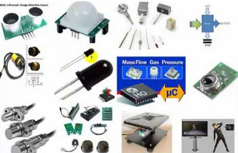

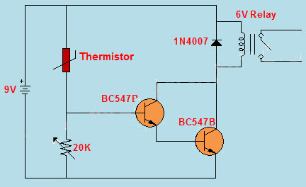
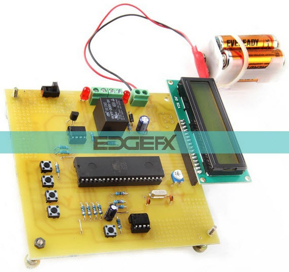


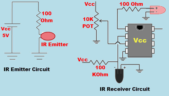

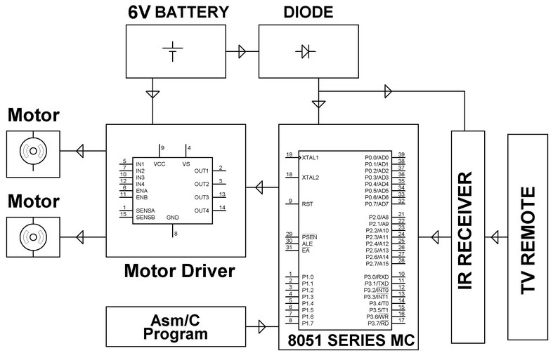
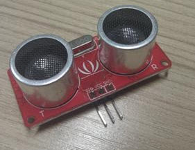
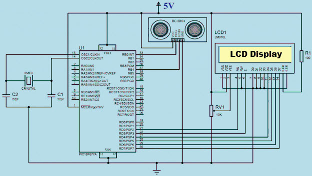

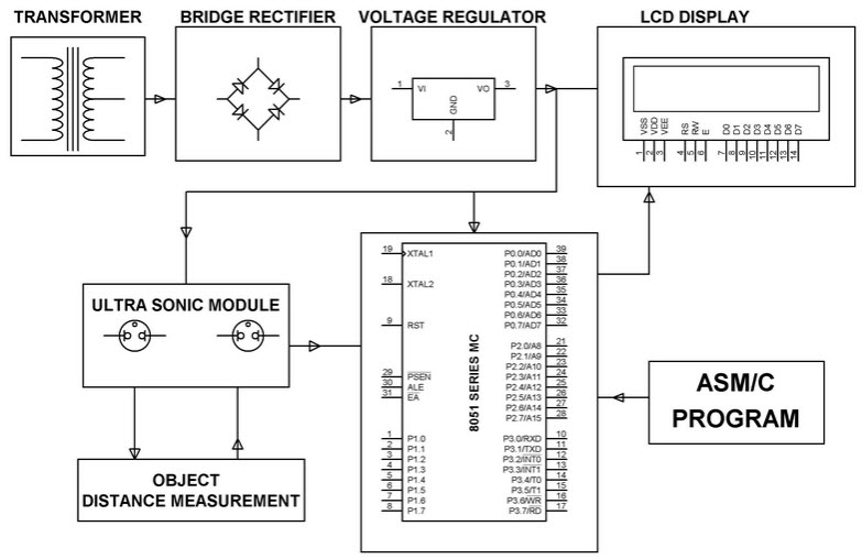

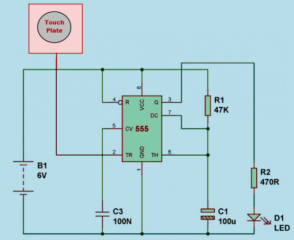


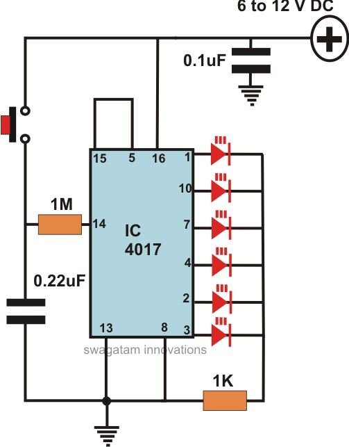


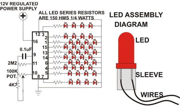
 Bimorph cantilevers used as micromechanical linear actuator:


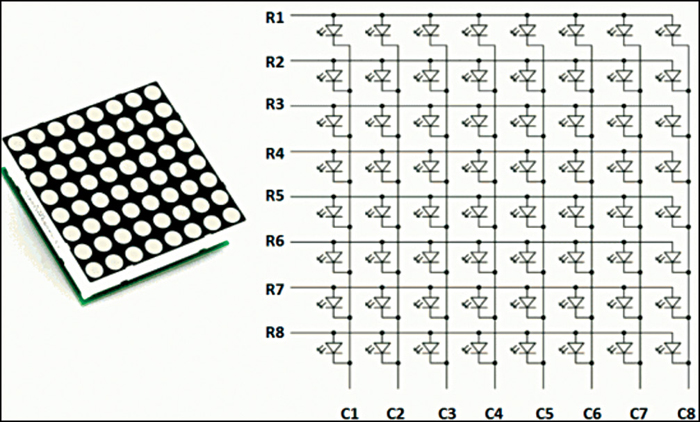
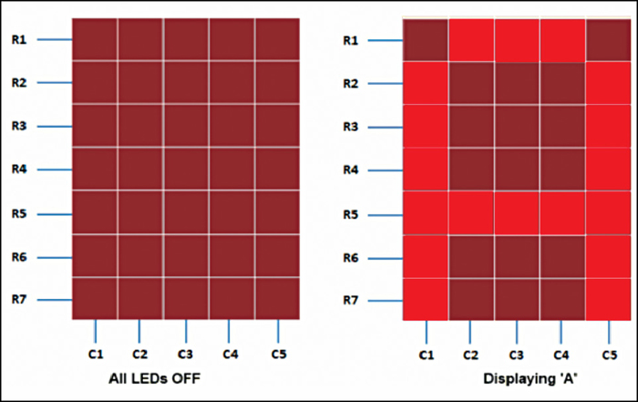
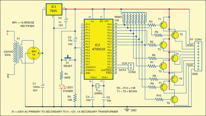
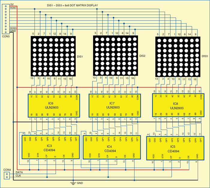
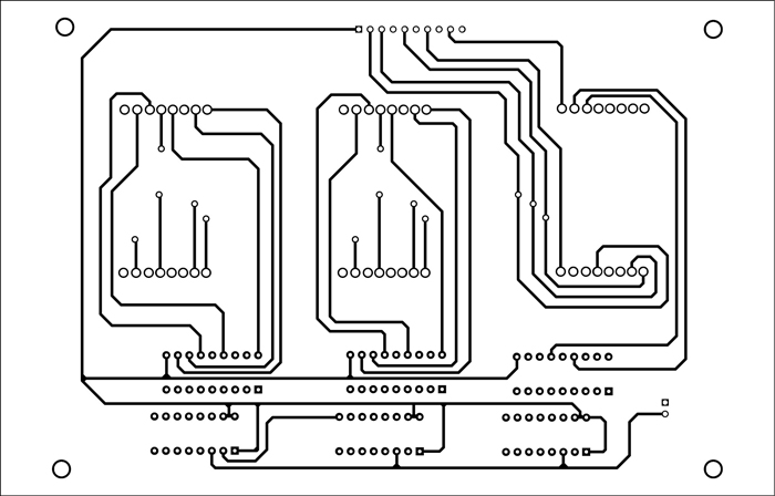
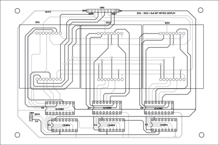
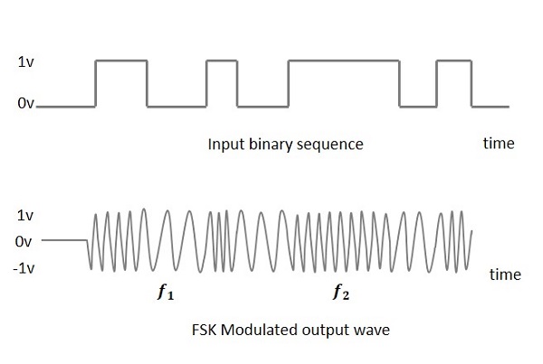
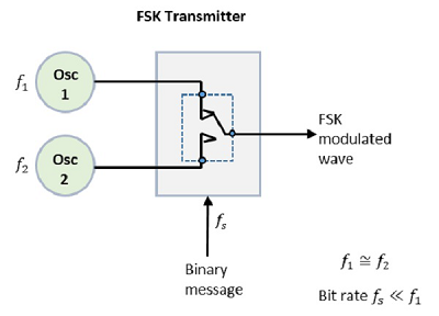
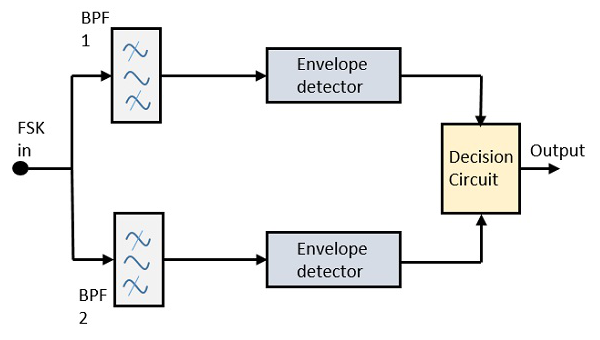
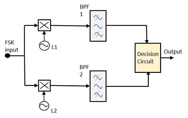
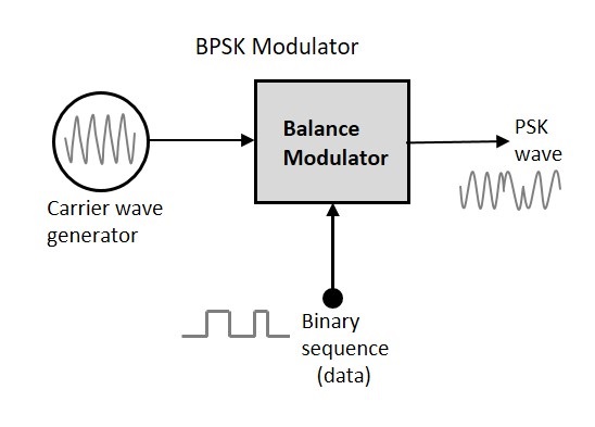
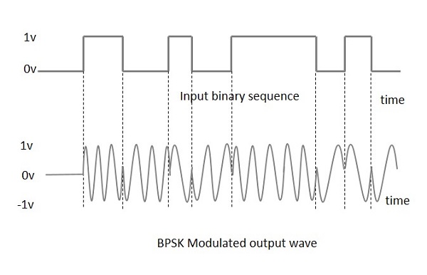
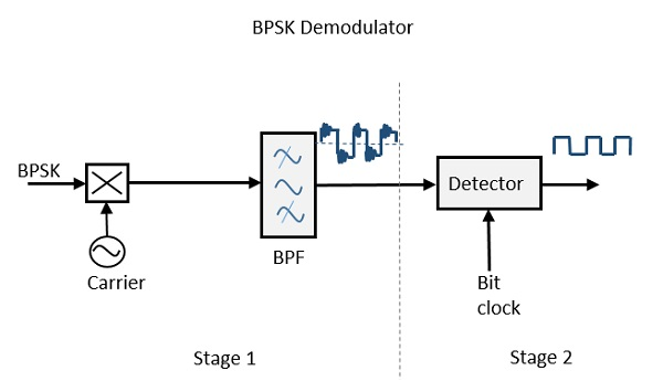
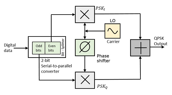
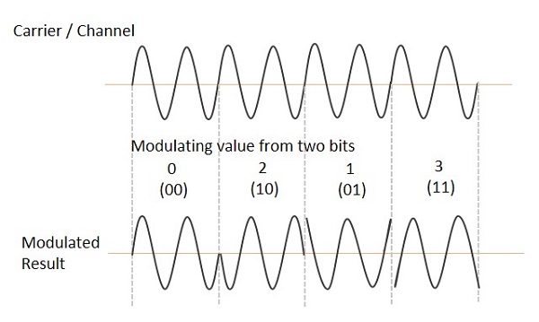
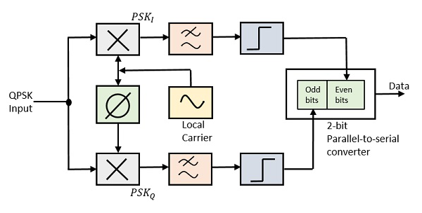
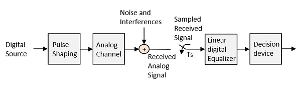


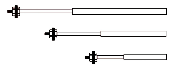
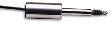
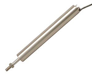
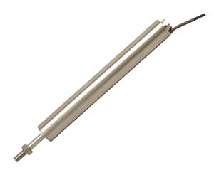
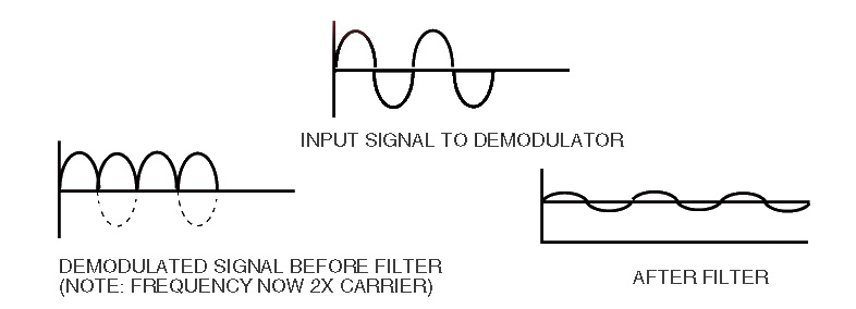
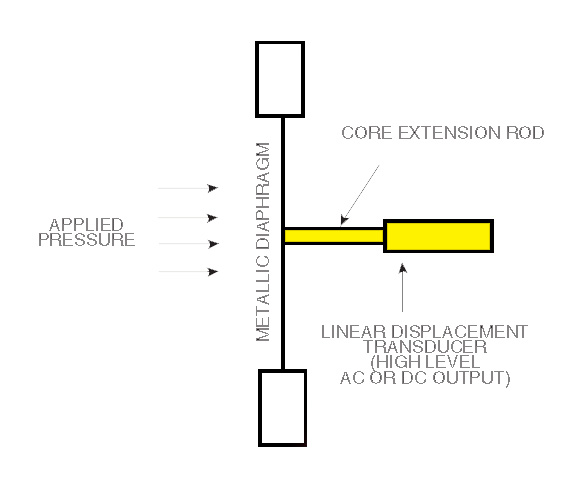
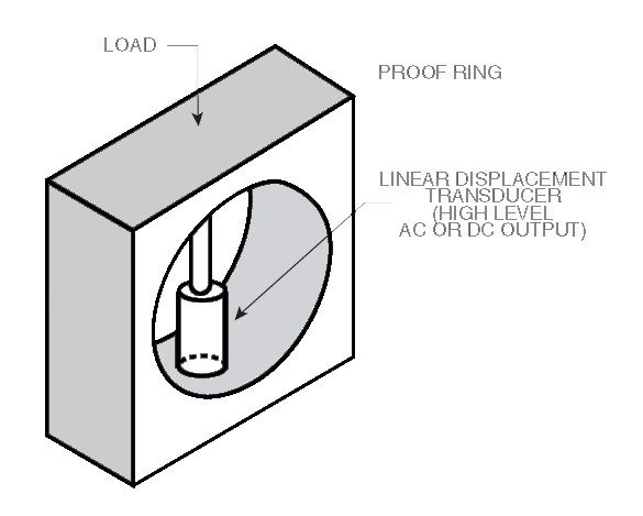

 The illustration on the right shows how the simple system described above would look in an actual transmission. The input shaft is connected to the ring gear (dark grey), The Output shaft is connected to the planet carrier (light grey) which is also connected to a “Multi-disk” clutch pack. The sun gear is connected to a drum (orange) which is also connected to the other half of the clutch pack. Surrounding the outside of the drum is a band (blue) that can be tightened around the drum when required to prevent the drum with the attached sun gear from turning.
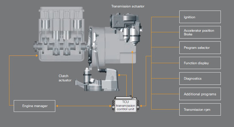
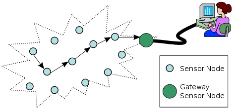


RFID Inlay Manufacturer
BalasHapus